Embed Size (px)
Citation preview
SSRNet: Scalable 3D Surface Reconstruction Network
Zhenxing Mi † Yiming Luo † Wenbing Tao ∗
National Key Laboratory of Science and Technology on Multi-spectral Information Processing
School of Artifical Intelligence and Automation, Huazhong University of Science and Technology, China
{m201772503, yiming luo, wenbingtao}@hust.edu.cn
Abstract
Existing learning-based surface reconstruction methods
from point clouds are still facing challenges in terms of
scalability and preservation of details on large-scale point
clouds. In this paper, we propose the SSRNet, a novel scal-
able learning-based method for surface reconstruction. The
proposed SSRNet constructs local geometry-aware features
for octree vertices and designs a scalable reconstruction
pipeline, which not only greatly enhances the predication
accuracy of the relative position between the vertices and
the implicit surface facilitating the surface reconstruction
quality, but also allows dividing the point cloud and octree
vertices and processing different parts in parallel for supe-
rior scalability on large-scale point clouds with millions of
points. Moreover, SSRNet demonstrates outstanding gen-
eralization capability and only needs several surface data
for training, much less than other learning-based recon-
struction methods, which can effectively avoid overfitting.
The trained model of SSRNet on one dataset can be directly
used on other datasets with superior performance. Finally,
the time consumption with SSRNet on a large-scale point
cloud is acceptable and competitive. To our knowledge, the
proposed SSRNet is the first to really bring a convincing so-
lution to the scalability issue of the learning-based surface
reconstruction methods, and is an important step to make
learning-based methods competitive with respect to geome-
try processing methods on real-world and challenging data.
Experiments show that our method achieves a breakthrough
in scalability and quality compared with state-of-the-art
learning-based methods.
1. Introduction
Point cloud is an important and widely used representa-
tion for 3D data. Surface reconstruction from point clouds
(SRPC) has been well studied in computer graphics. A lot
†Equal contribution∗Corresponding author
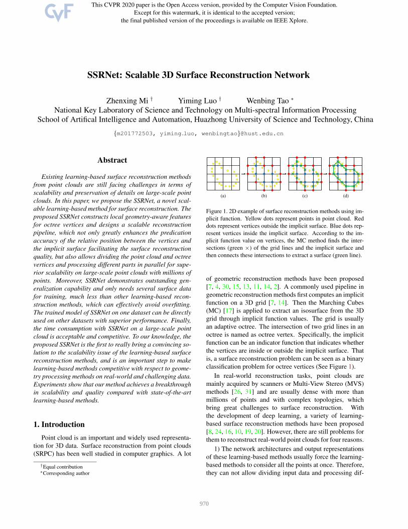
(d)(c)(b)(a)
Figure 1. 2D example of surface reconstruction methods using im-
plicit function. Yellow dots represent points in point cloud. Red
dots represent vertices outside the implicit surface. Blue dots rep-
resent vertices inside the implicit surface. According to the im-
plicit function value on vertices, the MC method finds the inter-
sections (green ×) of the grid lines and the implicit surface and
then connects these intersections to extract a surface (green line).
of geometric reconstruction methods have been proposed
[7, 4, 30, 15, 13, 11, 14, 2]. A commonly used pipeline in
geometric reconstruction methods first computes an implicit
function on a 3D grid [7, 14]. Then the Marching Cubes
(MC) [17] is applied to extract an isosurface from the 3D
grid through implicit function values. The grid is usually
an adaptive octree. The intersection of two grid lines in an
octree is named as octree vertex. Specifically, the implicit
function can be an indicator function that indicates whether
the vertices are inside or outside the implicit surface. That
is, a surface reconstruction problem can be seen as a binary
classification problem for octree vertices (See Figure 1).
In real-world reconstruction tasks, point clouds are
mainly acquired by scanners or Multi-View Stereo (MVS)
methods [26, 31] and are usually dense with more than
millions of points and with complex topologies, which
bring great challenges to surface reconstruction. With
the development of deep learning, a variety of learning-
based surface reconstruction methods have been proposed
[8, 24, 16, 10, 19, 20]. However, there are still problems for
them to reconstruct real-world point clouds for four reasons.
1) The network architectures and output representations
of these learning-based methods usually force the learning-
based methods to consider all the points at once. Therefore,
they can not allow dividing input data and processing dif-
970
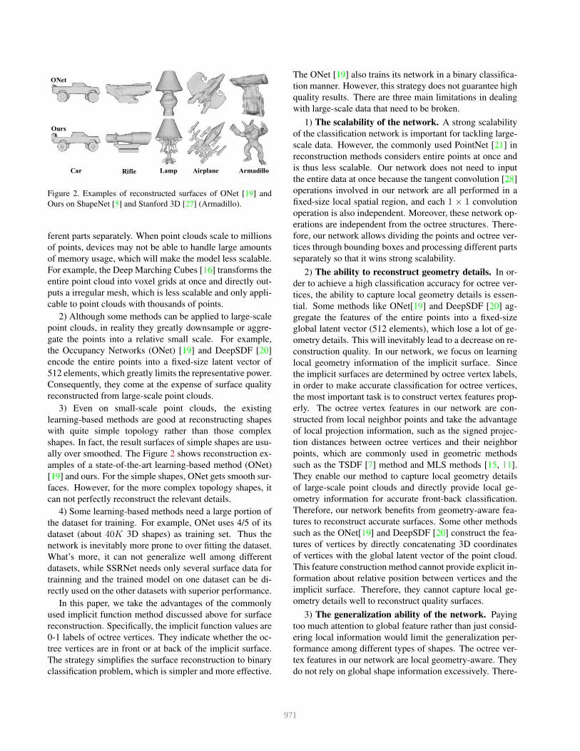
Lamp Airplane
ONet
Ours
Car ArmadilloRifle
Figure 2. Examples of reconstructed surfaces of ONet [19] and
Ours on ShapeNet [5] and Stanford 3D [27] (Armadillo).
ferent parts separately. When point clouds scale to millions
of points, devices may not be able to handle large amounts
of memory usage, which will make the model less scalable.
For example, the Deep Marching Cubes [16] transforms the
entire point cloud into voxel grids at once and directly out-
puts a irregular mesh, which is less scalable and only appli-
cable to point clouds with thousands of points.
2) Although some methods can be applied to large-scale
point clouds, in reality they greatly downsample or aggre-
gate the points into a relative small scale. For example,
the Occupancy Networks (ONet) [19] and DeepSDF [20]
encode the entire points into a fixed-size latent vector of
512 elements, which greatly limits the representative power.
Consequently, they come at the expense of surface quality
reconstructed from large-scale point clouds.
3) Even on small-scale point clouds, the existing
learning-based methods are good at reconstructing shapes
with quite simple topology rather than those complex
shapes. In fact, the result surfaces of simple shapes are usu-
ally over smoothed. The Figure 2 shows reconstruction ex-
amples of a state-of-the-art learning-based method (ONet)
[19] and ours. For the simple shapes, ONet gets smooth sur-
faces. However, for the more complex topology shapes, it
can not perfectly reconstruct the relevant details.
4) Some learning-based methods need a large portion of
the dataset for training. For example, ONet uses 4/5 of its
dataset (about 40K 3D shapes) as training set. Thus the
network is inevitably more prone to over fitting the dataset.
What’s more, it can not generalize well among different
datasets, while SSRNet needs only several surface data for
trainning and the trained model on one dataset can be di-
rectly used on the other datasets with superior performance.
In this paper, we take the advantages of the commonly
used implicit function method discussed above for surface
reconstruction. Specifically, the implicit function values are
0-1 labels of octree vertices. They indicate whether the oc-
tree vertices are in front or at back of the implicit surface.
The strategy simplifies the surface reconstruction to binary
classification problem, which is simpler and more effective.
The ONet [19] also trains its network in a binary classifica-
tion manner. However, this strategy does not guarantee high
quality results. There are three main limitations in dealing
with large-scale data that need to be broken.
1) The scalability of the network. A strong scalability
of the classification network is important for tackling large-
scale data. However, the commonly used PointNet [21] in
reconstruction methods considers entire points at once and
is thus less scalable. Our network does not need to input
the entire data at once because the tangent convolution [28]
operations involved in our network are all performed in a
fixed-size local spatial region, and each 1 × 1 convolution
operation is also independent. Moreover, these network op-
erations are independent from the octree structures. There-
fore, our network allows dividing the points and octree ver-
tices through bounding boxes and processing different parts
separately so that it wins strong scalability.
2) The ability to reconstruct geometry details. In or-
der to achieve a high classification accuracy for octree ver-
tices, the ability to capture local geometry details is essen-
tial. Some methods like ONet[19] and DeepSDF [20] ag-
gregate the features of the entire points into a fixed-size
global latent vector (512 elements), which lose a lot of ge-
ometry details. This will inevitably lead to a decrease on re-
construction quality. In our network, we focus on learning
local geometry information of the implicit surface. Since
the implicit surfaces are determined by octree vertex labels,
in order to make accurate classification for octree vertices,
the most important task is to construct vertex features prop-
erly. The octree vertex features in our network are con-
structed from local neighbor points and take the advantage
of local projection information, such as the signed projec-
tion distances between octree vertices and their neighbor
points, which are commonly used in geometric methods
such as the TSDF [7] method and MLS methods [15, 11].
They enable our method to capture local geometry details
of large-scale point clouds and directly provide local ge-
ometry information for accurate front-back classification.
Therefore, our network benefits from geometry-aware fea-
tures to reconstruct accurate surfaces. Some other methods
such as the ONet[19] and DeepSDF [20] construct the fea-
tures of vertices by directly concatenating 3D coordinates
of vertices with the global latent vector of the point cloud.
This feature construction method cannot provide explicit in-
formation about relative position between vertices and the
implicit surface. Therefore, they cannot capture local ge-
ometry details well to reconstruct quality surfaces.
3) The generalization ability of the network. Paying
too much attention to global feature rather than just consid-
ering local information would limit the generalization per-
formance among different types of shapes. The octree ver-
tex features in our network are local geometry-aware. They
do not rely on global shape information excessively. There-
971
fore, it has good generalization capability and does not need
too much training data, which avoids overfitting on dataset.
Overall, our contributions can be summarized as follows.
• We design a scalable pipeline for reconstructing sur-
face from real-world point clouds.
• We construct local geometry-aware octree vertex fea-
ture, which leads to accurate classification for octree
vertices and good generalization capability among dif-
ferent datasets.
Experiments have shown that our method achieves a sig-
nificant improvement in scalability and quality compared
with state-of-the-art learning-based methods, and is com-
petitive with respect to state-of-the-art geometric processing
methods in terms of reconstruction quality and efficiency 1.
2. Related Work
In this section, we first review some important geometric
reconstruction methods to introduce basic concepts. Then
we focus on existing learning-based surface reconstruction
methods. We mainly analyze whether they are able to scale
to large-scale datasets and to capture geometry details in
terms of network architectures and output representations.
2.1. Geometric reconstruction methods
Geometric reconstruction methods can be broadly cate-
gorized into global methods and local methods. The global
methods consider all the data at once, such as the radial ba-
sis functions (RBFs) methods [4, 30], and the (Screened)
Poisson Surface Reconstruction method (PSR) [13, 14].
The local fitting methods usually define a truncated
signed distance function (TSDF) [7] on a volumetric grid.
The various moving least squares methods (MLS) fit a lo-
cal distance field or vector fields by spatially varying low-
degree polynomials, and blend several nearby points to-
gether [15, 11]. The local projection and local least squares
fitting used by MLS are similar to the tangent convolution
used in our network. Local methods can be well scaled.
There are also other geometric methods with different
strategies, such as [2] computing restricted Voronoi cells.
More detailed reviews and evaluations of geometric meth-
ods can be found in [1] and [32].
2.2. Learningbased reconstruction methods
Network architecture. One straightforward network archi-
tecture for point clouds is to convert the point clouds into
regular 3D voxel grids or adaptive octree grids and apply 3D
convolutions [18, 23]. The voxel-based network used in 3D-
EPN [8] and the Deep Marching Cubes (DMC) [16] faces
cubic growth of computation and memory requirements for
1Our code will be available in Github later.
large-scale datasets. The OctNetFusion [24] and 3D-CFCN
[3] reconstruct implicit surface from multiple depth images
based on OctNet [23], a octree-based network, whose oper-
ations are complicated and are highly related to the octree
structure. Therefore, they also face computational issues in
reconstructing large-scale datasets.
Another type of network architecture learns point fea-
tures directly. The commonly used point cloud network is
PointNet [21]. It encodes global shape features into a latent
vector of fixed size. Some reconstruction methods also ex-
tract a latent vector from the point cloud, such as ONet [19]
and DeepSDF [20]. These networks are able to encode fea-
tures of a large-scale point cloud into a latent vector. How-
ever, the latent vector of a small size limits its representative
power for complex point clouds.
There are also network architectures learning local fea-
tures of point clouds. PointNet++ [22] groups points into
overlapping parts, then PointNet is chosen as the local fea-
ture learner for each part. The centroids of each parts are
selected using iterative farthest point sampling (FPS). The
points are grouped around the centroids by ball query that
finds all points within a radius to the query point. Using FPS
with grouping operations cannot be guaranteed to be per-
formed in a fixed-size spatial region. Therefore, the Point-
Net++ does not allow dividing input points using bounding
boxes and processing each part independently. The tangent
convolution network [28] learns local features from neigh-
bor points for semantic segmentation of 3D point clouds. It
defines three new network operations: tangent convolution,
pooling and unpooling. The neighbor points are collected
by ball query. The pooling and unpooling are implemented
via hashing onto a regular 3D grid. These operations are
performed in a fixed-size spatial region. Therefore, the tan-
gent convolution network can divide points using bounding
boxes and process each part independently.
Output representation. The scalability of learning-based
reconstruction methods is also greatly influenced by the out-
put representation. The reconstruction methods based on
voxel or octree grids usually use the occupancy or TSDF
on grids as the output representation. This output repre-
sentation, together with their network operations, is highly
related to the grid structure. Therefore, their scalability is
limited. The Deep Marching Cubes [16] and AtlasNet [10]
directly produce a triangular surface. The predictions of dif-
ferent parts of the surface are interdependent so they have
to consider the whole input point cloud at once.
ONet [19] and DeepSDF [20] learn shape-conditioned
classifiers whose decision boundary is the surface. Their
representations are similar to the front-back representation
of our SSRNet. Although ONet and DeepSDF support to
make predictions over 3D locations parallelly, they need to
get the global latent vector of the whole point cloud so they
do not allow dividing input points.
972
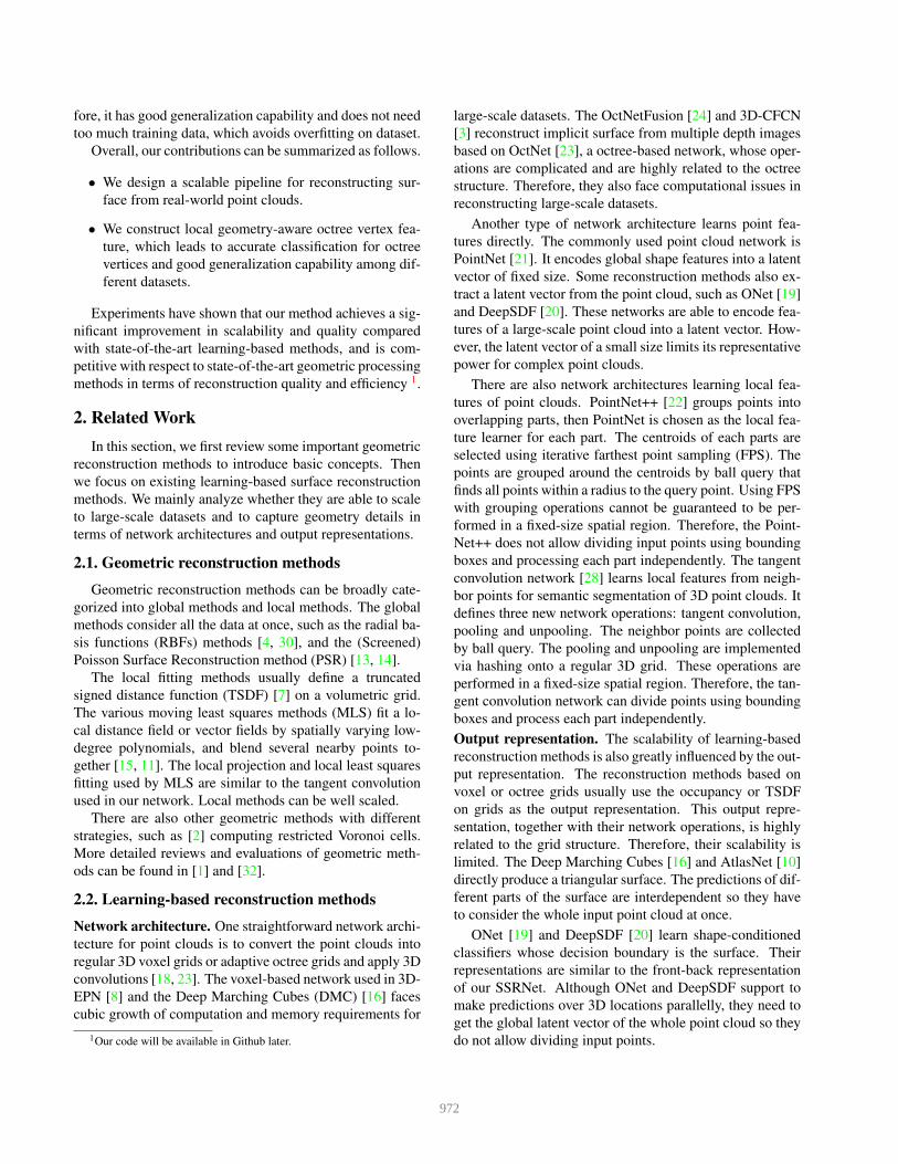
SSRNet
...
...
...
...
MC
& S
mooth
ing
Point Cloud
SSRNet
SSRNet
SSRNet
Vertex LabelsOctree Vertices
Points Vertices
Octree Vertex Labels Mesh
Figure 3. The pipeline of our method. Different parts are processed
by our SSRNet parallelly.
3. Method
3.1. Pipeline
We design a scalable learning-based surface reconstruc-
tion method, named SSRNet, which allows dividing the in-
put point clouds and octree vertices. Figure 3 shows the
pipeline of our method. Let P = {pi|i = 1, ..., N} be
the input point cloud of N points, where pi is point coor-
dinate with normal ni. We construct an octree from this
point cloud and extract the vertices V = {vi|i = 1, ...,M}of the finest level of this octree, where each vertex vi is
the coordinate. To prevent the whole input data exceed-
ing the GPU memory, we use bounding boxes to divide the
point cloud and the vertices into {Pj |j = 1, ...,K} and
{Vj |j = 1, ...,K}, where K is the number of boxes. The
bounding boxes of vertices are not overlapping. The corre-
sponding bounding boxes of points are larger than those of
octree vertices, which ensures that all the neighbor points
needed by vertices are included in the input. The border ef-
fects are thus largely suppressed. This enables our network
to make accurate predictions for vertices in the boundary of
the bounding box. We do not see any decay of accuracy on
the borders of vertex boxes. For the part j, the vertices Vj
and the corresponding points Pj are fed into SSRNet. The
SSRNet classifies each vertex vji in Vj as in front or at back
of the implicit surface represented by Pj . Let the function
represented by the network be fθ, where θ represents the
parameters of the network. Then the key of our method is
to classify vji in Vj . It can be formulated as:
fθ(Pj ,Vj , vji) → {0, 1} (1)
The front or back of an vertex is defined by the normal
direction of its nearest surface. The vertices are all from
the finest-level voxels of the octree in order to reconstruct
more details. They do not contain vertices far from the ac-
tual surface, which brings great challenges in classifying the
vertices. It is worth noting that the network operations in
SSRNet are not related to the structure of the octree. After
all the vertices are labeled, we extract surface using March-
ing Cubes (MC) and post-process the surface with a simple
Laplacian-based mesh smoothing method.
3.2. Geometryaware Vertex Feature
As discussed in the Introduction, the most important fea-
tures for octree vertex classification are signed projection
distances among octree vertices and their neighbor points.
In order to get accurate classification for octree vertices and
good generalization capability, we design geometry-aware
features for octree vertices directly encoding local projec-
tion information.
The tangent convolution [28] is defined as the 2D con-
volution on tangent images which are constructed by lo-
cal projections of neighbor points. The indices of the pro-
jected points used for tangent image can be precomputed,
which makes tangent convolution much more efficient. The
signals used in tangent images represent local surface ge-
ometry, including signed projection distances, normals, etc.
Therefore, it has the potential to encode local geometry fea-
tures for octree vertices.
However, there are problems in applying tangent convo-
lution to octree vertices directly. For a 3D location p, the
normal np of its tangent image is estimated through local
covariance analysis [25]. Let k be the eigenvector related to
the smallest eigenvalue of the covariance matrix of p. The
normal of tangent image is defined as k. Due to the direc-
tion of eigenvector k is ambiguous, it may not be consistent
with the real orientations of local implicit surfaces. The
signs of projection distances hence do not represent front-
back information accurately.
In order to solve this problem, we modify the definition
of np. Since the front-back classification is related to neigh-
bor points, we use the input normals of neighbor points as
additional constraints to define np. Let na be the average
input normal of the neighbor points of p. In our definition,
if the angle between eigenvector k and na is more than 90◦,
we invert the direction of k. Then we use it as the normal
np of the tangent image. That is, our definition of the tan-
gent image ensures that n⊤
pna > 0.
The features of octree vertices constructed by modified
tangent convolution directly encode front-back information.
They are local geometric features and not related to global
information of shapes, so our network is scalable and can
generalize well among different datasets. It’s worth noting
that we use neighbor points in the point cloud rather than
neighbor vertices to compute the tangent images. It is be-
cause our network classifies octree vertices with respect to
the surface represented by points from P , rather than being
represented by neighbor vertices.
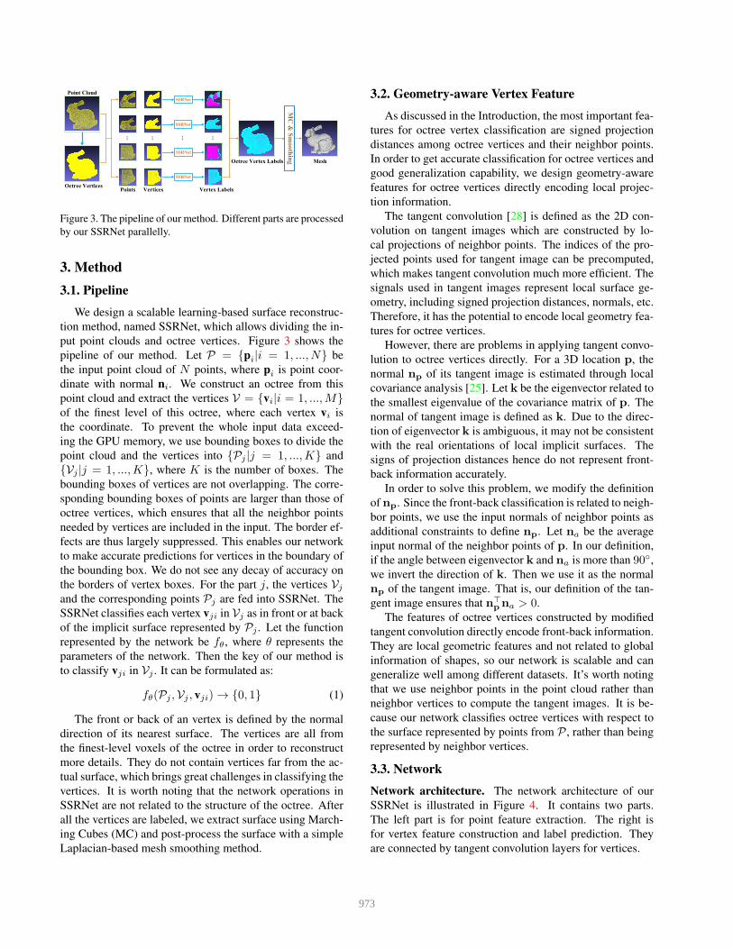
3.3. Network
Network architecture. The network architecture of our
SSRNet is illustrated in Figure 4. It contains two parts.
The left part is for point feature extraction. The right is
for vertex feature construction and label prediction. They
are connected by tangent convolution layers for vertices.
973
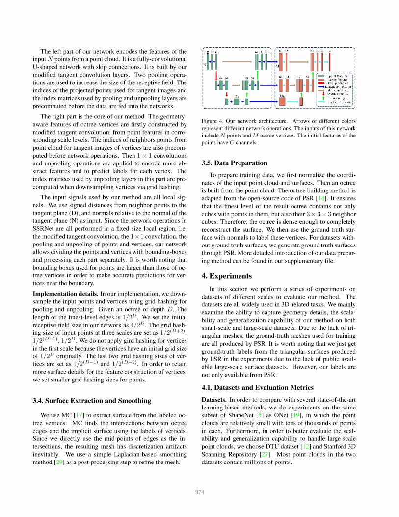
The left part of our network encodes the features of the
input N points from a point cloud. It is a fully-convolutional
U-shaped network with skip connections. It is built by our
modified tangent convolution layers. Two pooling opera-
tions are used to increase the size of the receptive field. The
indices of the projected points used for tangent images and
the index matrices used by pooling and unpooling layers are
precomputed before the data are fed into the networks.
The right part is the core of our method. The geometry-
aware features of octree vertices are firstly constructed by
modified tangent convolution, from point features in corre-
sponding scale levels. The indices of neighbors points from
point cloud for tangent images of vertices are also precom-
puted before network operations. Then 1 × 1 convolutions
and unpooling operations are applied to encode more ab-
stract features and to predict labels for each vertex. The
index matrices used by unpooling layers in this part are pre-
computed when downsampling vertices via grid hashing.
The input signals used by our method are all local sig-
nals. We use signed distances from neighbor points to the
tangent plane (D), and normals relative to the normal of the
tangent plane (N) as input. Since the network operations in
SSRNet are all performed in a fixed-size local region, i.e.
the modified tangent convolution, the 1×1 convolution, the
pooling and unpooling of points and vertices, our network
allows dividing the points and vertices with bounding-boxes
and processing each part separately. It is worth noting that
bounding boxes used for points are larger than those of oc-
tree vertices in order to make accurate predictions for ver-
tices near the boundary.
Implementation details. In our implementation, we down-
sample the input points and vertices using grid hashing for
pooling and unpooling. Given an octree of depth D, The
length of the finest-level edges is 1/2D. We set the initial
receptive field size in our network as 4/2D. The grid hash-
ing size of input points at three scales are set as 1/2(D+2),
1/2(D+1), 1/2D. We do not apply gird hashing for vertices
in the first scale because the vertices have an initial grid size
of 1/2D originally. The last two grid hashing sizes of ver-
tices are set as 1/2(D−1) and 1/2(D−2). In order to retain
more surface details for the feature construction of vertices,
we set smaller grid hashing sizes for points.
3.4. Surface Extraction and Smoothing
We use MC [17] to extract surface from the labeled oc-
tree vertices. MC finds the intersections between octree
edges and the implicit surface using the labels of vertices.
Since we directly use the mid-points of edges as the in-
tersections, the resulting mesh has discretization artifacts
inevitably. We use a simple Laplacian-based smoothing
method [29] as a post-processing step to refine the mesh.
Figure 4. Our network architecture. Arrows of different colors
represent different network operations. The inputs of this network
include N points and M octree vertices. The initial features of the
points have C channels.
3.5. Data Preparation
To prepare training data, we first normalize the coordi-
nates of the input point cloud and surfaces. Then an octree
is built from the point cloud. The octree building method is
adapted from the open-source code of PSR [14]. It ensures
that the finest level of the result octree contains not only
cubes with points in them, but also their 3× 3× 3 neighbor
cubes. Therefore, the octree is dense enough to completely
reconstruct the surface. We then use the ground truth sur-
face with normals to label these vertices. For datasets with-
out ground truth surfaces, we generate ground truth surfaces
through PSR. More detailed introduction of our data prepar-
ing method can be found in our supplementary file.
4. Experiments
In this section we perform a series of experiments on
datasets of different scales to evaluate our method. The
datasets are all widely used in 3D-related tasks. We mainly
examine the ability to capture geometry details, the scala-
bility and generalization capability of our method on both
small-scale and large-scale datasets. Due to the lack of tri-
angular meshes, the ground-truth meshes used for training
are all produced by PSR. It is worth noting that we just get
ground-truth labels from the triangular surfaces produced
by PSR in the experiments due to the lack of public avail-
able large-scale surface datasets. However, our labels are
not only available from PSR.
4.1. Datasets and Evaluation Metrics
Datasets. In order to compare with several state-of-the-art
learning-based methods, we do experiments on the same
subset of ShapeNet [5] as ONet [19], in which the point
clouds are relatively small with tens of thousands of points
in each. Furthermore, in order to better evaluate the scal-
ability and generalization capability to handle large-scale
point clouds, we choose DTU dataset [12] and Stanford 3D
Scanning Repository [27]. Most point clouds in the two
datasets contain millions of points.
974

Display Rifle
Ground Truth Model
ONet
Ours
Chair TelephoneTableCabinet LampVesselAirplaneBenchSofaCar Loud
Speaker
Figure 5. Examples of reconstructed surfaces on testing set of ShapeNet [5] by ONet [19] and our method.
Table 1. Classification Accuracy of SSRNet on Datasets of differ-
ent scales. ShapeNet-Model and DTU-Model represent the models
we trained on ShapeNet [5] and DTU [12] respectively.
Dataset ShapeNet [5] DTU [12]Stanford [27]
ShapeNet-Model DTU-Model
Accuracy (%) 97.6 95.7 98.1 98.2
Evaluation Metrics. The direct metric of our network is
the classification accuracy of octree vertices. It is worth
mentioning that the vertices in our experiments are all from
the finest-level voxels of the octree. With octree of rela-
tively high resolution, these voxels do not contain vertices
very far from the actual surface. Therefore, a high clas-
sification accuracy matters a lot to the quality of the final
mesh. For mesh comparison on ShapeNet, we use the same
evaluation metrics with ONet, including the volumetric IoU
(higher is better), the Chamfer-L1 distance (lower is better)
and the normal consistency score (higher is better). On the
DTU dataset, we use DTU evaluation method [12], which
mainly evaluates DTU Accuracy and DTU Completeness
(both lower is better). And for Stanford datasets, Chamfer
distance (CD) (lower is better) is adopted in order to eval-
uate the points of the output meshes, and the CD is also
taken into consideration in the evaluation on DTU dataset.
For each point in a cloud, CD finds the nearest point in the
other point cloud, and averages the square of distances up.
4.2. Results on Shapenet
In our first experiment, we evaluate the capacity of our
network to capture shape details on ShapeNet. We use the
same test split as ONet for fair comparisons. The testing
set contains about 10K shapes. We only randomly select a
subset from the training set of ONet for training. The train-
ing set of our method (4K shapes) is 1/10 of the training
set of ONet (40K shapes). We do not use a large amount
of training data as ONet did mainly for two reasons. On the
one hand, it is necessary to eliminate the possibility of over-
fitting a dataset due to too much training data. On the other
hand, our network learns local geometry-aware features so
that it can capture more geometry details with less training
data. Therefore, it is unnecessary for us to use too many
training samples.
In our experiments, each point cloud in training and test-
ing set contains 100K points. We add Gaussian noise with
zero mean and standard deviation 0.05 to the point clouds
as ONet did. Our network is efficient at processing point
clouds with a large number of points, so we do not down-
sample the point clouds. We think it is important for Sur-
face Reconstruction from Point Clouds (SRPC) methods to
be adaptive to the original data, rather than reducing the
amount of input data and the resolution to fit their networks.
After all, the representative power of 300 points used by
ONet is really limited. The original synthetic models of
ShapeNet do not have consistent normals so that we recon-
struct surfaces from the ground truth point clouds using PSR
on octrees of depth 9 to generate the training data. We use
octrees of depth 8 in SSRNet for training and testing.
For mesh comparison, we use the evaluation metrics on
ShapeNet mentioned in Section 4.1, including the volumet-
ric IoU, the Chamfer-L1 distance and the normal consis-
tency score. We evaluate all shapes in the testing set on
these metrics. The results of existing learning based 3D re-
construction approaches, i.e. the 3D-R2N2 [6], PSGN [9],
Deep Marching Cubes (DMC) [16] and ONet [19], are ob-
tained from the paper of ONet. As mentioned in ONet, it
is not possible to evaluate the IoU for PSGN for the rea-
son that it does not yield watertight meshes. ONet adapted
3D-R2N2 and PSGN for point cloud input by changing the
encoders. Although methods in Table 2 use different strate-
gies, they actually solve the same task of SRPC. Quantita-
tive results are shown in Table 2.
The classification accuracy of octree vertices on
ShapeNet dataset shows strong robustness of our network.
It achieves high classification accuracy of 97.6% on noisy
point clouds (See Table 1). The Table 2 shows that our
method gets great improvements on these metrics. Com-
pared with the best performance of other methods, we
achieve the highest IoU, lower Chamfer-L1 distance and
higher normal consistency. More specifically, the IoU of our
results is about 18% higher than that of ONet. It is worth
noting that our network has only 0.49 million parameters,
975
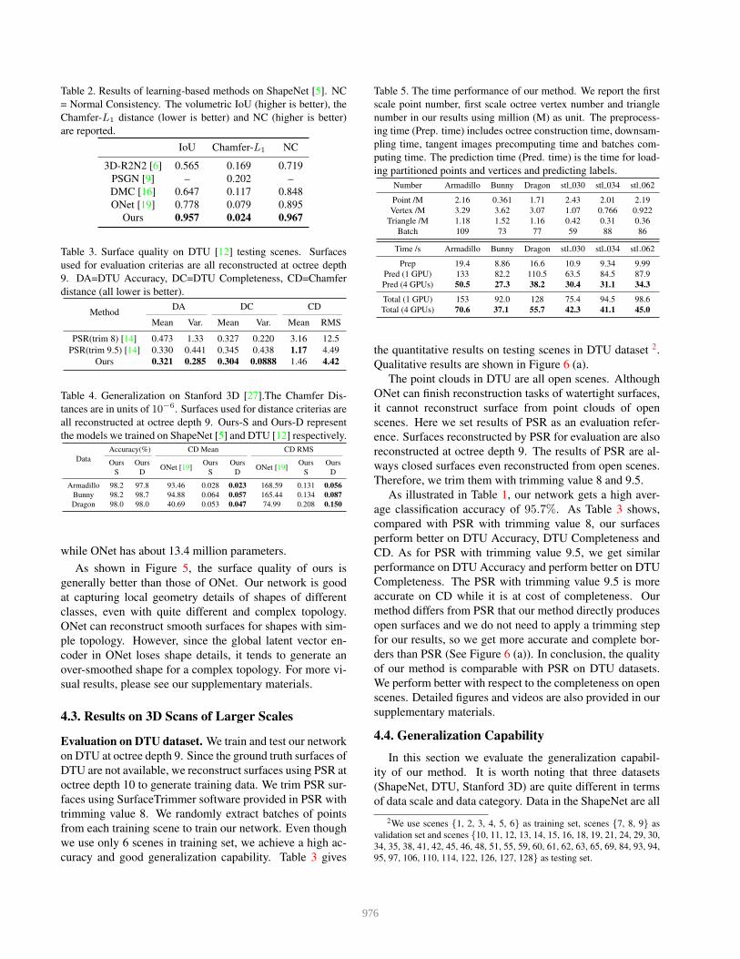
Table 2. Results of learning-based methods on ShapeNet [5]. NC
= Normal Consistency. The volumetric IoU (higher is better), the
Chamfer-L1 distance (lower is better) and NC (higher is better)
are reported.
IoU Chamfer-L1 NC
3D-R2N2 [6] 0.565 0.169 0.719
PSGN [9] – 0.202 –
DMC [16] 0.647 0.117 0.848
ONet [19] 0.778 0.079 0.895
Ours 0.957 0.024 0.967
Table 3. Surface quality on DTU [12] testing scenes. Surfaces
used for evaluation criterias are all reconstructed at octree depth
9. DA=DTU Accuracy, DC=DTU Completeness, CD=Chamfer
distance (all lower is better).
MethodDA DC CD
Mean Var. Mean Var. Mean RMS
PSR(trim 8) [14] 0.473 1.33 0.327 0.220 3.16 12.5
PSR(trim 9.5) [14] 0.330 0.441 0.345 0.438 1.17 4.49
Ours 0.321 0.285 0.304 0.0888 1.46 4.42
Table 4. Generalization on Stanford 3D [27].The Chamfer Dis-
tances are in units of 10−6. Surfaces used for distance criterias are
all reconstructed at octree depth 9. Ours-S and Ours-D represent
the models we trained on ShapeNet [5] and DTU [12] respectively.
Data
Accuracy(%) CD Mean CD RMS
Ours OursONet [19]
Ours OursONet [19]
Ours Ours
S D S D S D
Armadillo 98.2 97.8 93.46 0.028 0.023 168.59 0.131 0.056
Bunny 98.2 98.7 94.88 0.064 0.057 165.44 0.134 0.087
Dragon 98.0 98.0 40.69 0.053 0.047 74.99 0.208 0.150
while ONet has about 13.4 million parameters.
As shown in Figure 5, the surface quality of ours is
generally better than those of ONet. Our network is good
at capturing local geometry details of shapes of different
classes, even with quite different and complex topology.
ONet can reconstruct smooth surfaces for shapes with sim-
ple topology. However, since the global latent vector en-
coder in ONet loses shape details, it tends to generate an
over-smoothed shape for a complex topology. For more vi-
sual results, please see our supplementary materials.
4.3. Results on 3D Scans of Larger Scales
Evaluation on DTU dataset. We train and test our network
on DTU at octree depth 9. Since the ground truth surfaces of
DTU are not available, we reconstruct surfaces using PSR at
octree depth 10 to generate training data. We trim PSR sur-
faces using SurfaceTrimmer software provided in PSR with
trimming value 8. We randomly extract batches of points
from each training scene to train our network. Even though
we use only 6 scenes in training set, we achieve a high ac-
curacy and good generalization capability. Table 3 gives
Table 5. The time performance of our method. We report the first
scale point number, first scale octree vertex number and triangle
number in our results using million (M) as unit. The preprocess-
ing time (Prep. time) includes octree construction time, downsam-
pling time, tangent images precomputing time and batches com-
puting time. The prediction time (Pred. time) is the time for load-
ing partitioned points and vertices and predicting labels.
Number Armadillo Bunny Dragon stl 030 stl 034 stl 062
Point /M 2.16 0.361 1.71 2.43 2.01 2.19
Vertex /M 3.29 3.62 3.07 1.07 0.766 0.922
Triangle /M 1.18 1.52 1.16 0.42 0.31 0.36
Batch 109 73 77 59 88 86
Time /s Armadillo Bunny Dragon stl 030 stl 034 stl 062
Prep 19.4 8.86 16.6 10.9 9.34 9.99
Pred (1 GPU) 133 82.2 110.5 63.5 84.5 87.9
Pred (4 GPUs) 50.5 27.3 38.2 30.4 31.1 34.3
Total (1 GPU) 153 92.0 128 75.4 94.5 98.6
Total (4 GPUs) 70.6 37.1 55.7 42.3 41.1 45.0
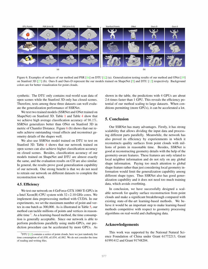
the quantitative results on testing scenes in DTU dataset 2.
Qualitative results are shown in Figure 6 (a).
The point clouds in DTU are all open scenes. Although
ONet can finish reconstruction tasks of watertight surfaces,
it cannot reconstruct surface from point clouds of open
scenes. Here we set results of PSR as an evaluation refer-
ence. Surfaces reconstructed by PSR for evaluation are also
reconstructed at octree depth 9. The results of PSR are al-
ways closed surfaces even reconstructed from open scenes.
Therefore, we trim them with trimming value 8 and 9.5.
As illustrated in Table 1, our network gets a high aver-
age classification accuracy of 95.7%. As Table 3 shows,
compared with PSR with trimming value 8, our surfaces
perform better on DTU Accuracy, DTU Completeness and
CD. As for PSR with trimming value 9.5, we get similar
performance on DTU Accuracy and perform better on DTU
Completeness. The PSR with trimming value 9.5 is more
accurate on CD while it is at cost of completeness. Our
method differs from PSR that our method directly produces
open surfaces and we do not need to apply a trimming step
for our results, so we get more accurate and complete bor-
ders than PSR (See Figure 6 (a)). In conclusion, the quality
of our method is comparable with PSR on DTU datasets.
We perform better with respect to the completeness on open
scenes. Detailed figures and videos are also provided in our
supplementary materials.
4.4. Generalization Capability
In this section we evaluate the generalization capabil-
ity of our method. It is worth noting that three datasets
(ShapeNet, DTU, Stanford 3D) are quite different in terms
of data scale and data category. Data in the ShapeNet are all
2We use scenes {1, 2, 3, 4, 5, 6} as training set, scenes {7, 8, 9} as
validation set and scenes {10, 11, 12, 13, 14, 15, 16, 18, 19, 21, 24, 29, 30,
34, 35, 38, 41, 42, 45, 46, 48, 51, 55, 59, 60, 61, 62, 63, 65, 69, 84, 93, 94,
95, 97, 106, 110, 114, 122, 126, 127, 128} as testing set.
976
Stl_030
Stl_034
Stl_062
Armadillo
Bunny
Dragon
DTU Points PSR (trim 8) PSR (trim 9.5) Ours Stanford Points ONet Ours-D Ours-S
(a) (b)
Figure 6. Examples of surfaces of our method and PSR [14] on DTU [12] (a). Generalization testing results of our method and ONet [19]
on Stanford 3D [27] (b). Ours-S and Ours-D represent the our models trained on ShapeNet [5] and DTU [12] respectively. Background
colors are for better visualization for point clouds.
synthetic. The DTU only contains real-world scan data of
open scenes while the Stanford 3D only has closed scenes.
Therefore, tests among these three datasets can well evalu-
ate the generalization performance of SSRNet.
We test two trained models (SSRNet and ONet trained on
ShapeNet) on Stanford 3D. Table 1 and Table 4 show that
we achieve high average classification accuracy of 98.1%.
SSRNet generalizes better than ONet on Stanford 3D in
metric of Chamfer Distance. Figure 6 (b) shows that our re-
sults achieve outstanding visual effects and reconstruct ge-
ometry details of the shapes well.
We also use SSRNet model trained on DTU to test on
Stanford 3D. Table 4 shows that our network trained on
open scenes can also achieve higher classification accuracy
on closed scenes. Besides, classification accuracy of our
models trained on ShapeNet and DTU are almost exactly
the same, and the evaluation results on CD are also similar.
In general, the results prove good generalization capability
of our network. One strong benefit is that we do not need
to retrain our network on different datasets to complete the
reconstruction work.
4.5. Efficiency
We test our network on 4 GeForce GTX 1080 Ti GPUs in
a Intel Xeon(R) CPU system with 32×2.10 GHz cores. We
implement data preprocessing method with CUDA. In our
experiments, we set the maximum number of point and ver-
tex in one batch as 300,000. As is illustrated in Table 5, our
method can tackle millions of points and vertices in reason-
able time 3. As a learning-based method, the time consump-
tion is generally acceptable. Since our network is able to
perform predictions parallelly using multi-GPUs, our pre-
diction procedure can be accelerated by more GPUs. As
3DTU [12] contains a series of point clouds, here we just randomly list
time consumption of stl 030, stl 034, stl 062. We do not consider the time
of reading and writing files.
shown in the table, the predictions with 4 GPUs are about
2.6 times faster than 1 GPU. This reveals the efficiency po-
tential of our method scaling to large datasets. When con-
ditions permitting (more GPUs), it can be accelerated a lot.
5. Conclusion
Our SSRNet has many advantages. Firstly, it has strong
scalability that allows dividing the input data and process-
ing different parts parallelly. Meanwhile, the network has
also proved its efficiency by experienments in which it
reconstructs quality surfaces from point clouds with mil-
lions of points in reasonable time. Besides, SSRNet is
good at reconstructing geometry details with the help of the
geometry-aware features. These features are only related to
local neighbor information and do not rely on any global
shape information. Paying too much attention to global
shape feature rather than just considering local geometry in-
formation would limit the generalization capability among
different shape types. Thus SSRNet also has good gener-
alization capability and it does not need too much training
data, which avoids overfitting.
In conclusion, we have successfully designed a scal-
able network for quality surface reconstruction from point
clouds and make a significant breakthrough compared with
existing state-of-the-art learning-based methods. We be-
lieve it would be an important step to make learning-based
methods competitive with respect to geometry processing
algorithms on real-world and challenging data.
Acknowledgements
This work was supported by the National Natural Sci-
ence Foundation of China under Grant 61772213, Grant
61991412 and Grant 91748204.
977
References
[1] Matthew Berger, Andrea Tagliasacchi, Lee Seversky, Pierre
Alliez, Joshua Levine, Andrei Sharf, and Claudio Silva. State
of the art in surface reconstruction from point clouds. 2014.
3
[2] Dobrina Boltcheva and Bruno Levy. Surface reconstruction
by computing restricted voronoi cells in parallel. Computer-
Aided Design, 90:123–134, 2017. 1, 3
[3] Yan-Pei Cao, Zheng-Ning Liu, Zheng-Fei Kuang, Leif
Kobbelt, and Shi-Min Hu. Learning to reconstruct high-
quality 3d shapes with cascaded fully convolutional net-
works. In Proceedings of the European Conference on Com-
puter Vision (ECCV), pages 616–633, 2018. 3
[4] Jonathan C Carr, Richard K Beatson, Jon B Cherrie, Tim J
Mitchell, W Richard Fright, Bruce C McCallum, and Tim R
Evans. Reconstruction and representation of 3d objects with
radial basis functions. In Proceedings of the 28th annual con-
ference on Computer graphics and interactive techniques,
pages 67–76. ACM, 2001. 1, 3
[5] Angel X Chang, Thomas Funkhouser, Leonidas Guibas,
Pat Hanrahan, Qixing Huang, Zimo Li, Silvio Savarese,
Manolis Savva, Shuran Song, Hao Su, et al. Shapenet:
An information-rich 3d model repository. arXiv preprint
arXiv:1512.03012, 2015. 2, 5, 6, 7, 8
[6] Christopher B Choy, Danfei Xu, JunYoung Gwak, Kevin
Chen, and Silvio Savarese. 3d-r2n2: A unified approach
for single and multi-view 3d object reconstruction. In Eu-
ropean conference on computer vision (ECCV), pages 628–
644. Springer, 2016. 6, 7
[7] Brian Curless and Marc Levoy. A volumetric method for
building complex models from range images. 1996. 1, 2, 3
[8] Angela Dai, Charles Ruizhongtai Qi, and Matthias Nießner.
Shape completion using 3d-encoder-predictor cnns and
shape synthesis. In Proceedings of the IEEE Conference
on Computer Vision and Pattern Recognition (CVPR), pages
5868–5877, 2017. 1, 3
[9] Haoqiang Fan, Hao Su, and Leonidas J Guibas. A point set
generation network for 3d object reconstruction from a sin-
gle image. In Proceedings of the IEEE Conference on Com-
puter Vision and Pattern Recognition (CVPR), pages 605–
613, 2017. 6, 7
[10] Thibault Groueix, Matthew Fisher, Vladimir G Kim,
Bryan C Russell, and Mathieu Aubry. A papier-mache ap-
proach to learning 3d surface generation. In Proceedings
of the IEEE Conference on Computer Vision and Pattern
Recognition (CVPR), pages 216–224, 2018. 1, 3
[11] Gael Guennebaud and Markus Gross. Algebraic point set
surfaces. In ACM Transactions on Graphics (TOG), vol-
ume 26, page 23. ACM, 2007. 1, 2, 3
[12] Rasmus Jensen, Anders Dahl, George Vogiatzis, Engil Tola,
and Henrik Aanæs. Large scale multi-view stereopsis eval-
uation. In 2014 IEEE Conference on Computer Vision and
Pattern Recognition, pages 406–413. IEEE, 2014. 5, 6, 7, 8
[13] Michael Kazhdan, Matthew Bolitho, and Hugues Hoppe.
Poisson surface reconstruction. In Proceedings of the
fourth Eurographics symposium on Geometry processing,
volume 7, 2006. 1, 3
[14] Michael Kazhdan and Hugues Hoppe. Screened poisson sur-
face reconstruction. ACM Transactions on Graphics (ToG),
32(3):29, 2013. 1, 3, 5, 7, 8
[15] David Levin. Mesh-independent surface interpolation. In
Geometric modeling for scientific visualization, pages 37–
49. Springer, 2004. 1, 2, 3
[16] Yiyi Liao, Simon Donne, and Andreas Geiger. Deep march-
ing cubes: Learning explicit surface representations. In Pro-
ceedings of the IEEE Conference on Computer Vision and
Pattern Recognition (CVPR), pages 2916–2925, 2018. 1, 2,
3, 6, 7
[17] William E Lorensen and Harvey E Cline. Marching cubes:
A high resolution 3d surface construction algorithm. In ACM
siggraph computer graphics, volume 21, pages 163–169.
ACM, 1987. 1, 5
[18] Daniel Maturana and Sebastian Scherer. Voxnet: A 3d con-
volutional neural network for real-time object recognition.
In 2015 IEEE/RSJ International Conference on Intelligent
Robots and Systems (IROS), pages 922–928. IEEE, 2015. 3
[19] Lars Mescheder, Michael Oechsle, Michael Niemeyer, Se-
bastian Nowozin, and Andreas Geiger. Occupancy networks:
Learning 3d reconstruction in function space. In Proceed-
ings of the IEEE Conference on Computer Vision and Pattern
Recognition, pages 4460–4470, 2019. 1, 2, 3, 5, 6, 7, 8
[20] Jeong Joon Park, Peter Florence, Julian Straub, Richard
Newcombe, and Steven Lovegrove. Deepsdf: Learning con-
tinuous signed distance functions for shape representation.
In Proceedings of the IEEE Conference on Computer Vision
and Pattern Recognition, pages 165–174, 2019. 1, 2, 3
[21] Charles R Qi, Hao Su, Kaichun Mo, and Leonidas J Guibas.
Pointnet: Deep learning on point sets for 3d classification
and segmentation. In Proceedings of the IEEE Conference
on Computer Vision and Pattern Recognition (CVPR), pages
652–660, 2017. 2, 3
[22] Charles Ruizhongtai Qi, Li Yi, Hao Su, and Leonidas J
Guibas. Pointnet++: Deep hierarchical feature learning on
point sets in a metric space. In Advances in Neural Informa-
tion Processing Systems, pages 5099–5108, 2017. 3
[23] Gernot Riegler, Ali Osman Ulusoy, and Andreas Geiger.
Octnet: Learning deep 3d representations at high resolutions.
In Proceedings of the IEEE Conference on Computer Vision
and Pattern Recognition (CVPR), pages 3577–3586, 2017. 3
[24] Gernot Riegler, Ali Osman Ulusoy, Horst Bischof, and An-
dreas Geiger. Octnetfusion: Learning depth fusion from data.
In 2017 International Conference on 3D Vision (3DV), pages
57–66. IEEE, 2017. 1, 3
[25] Samuele Salti, Federico Tombari, and Luigi Di Stefano.
Shot: Unique signatures of histograms for surface and tex-
ture description. Computer Vision and Image Understand-
ing, 125:251–264, 2014. 4
[26] Johannes L Schonberger, Enliang Zheng, Jan-Michael
Frahm, and Marc Pollefeys. Pixelwise view selection for
unstructured multi-view stereo. In Proceedings of the Euro-
pean Conference on Computer Vision (ECCV), pages 501–
518. Springer, 2016. 1
[27] Stanford 3D. The stanford 3d scanning repository, 2013. 2,
5, 6, 7, 8
978
[28] Maxim Tatarchenko, Jaesik Park, Vladlen Koltun, and Qian-
Yi Zhou. Tangent convolutions for dense prediction in 3d.
In Proceedings of the IEEE Conference on Computer Vision
and Pattern Recognition (CVPR), pages 3887–3896, 2018.
2, 3, 4
[29] Gabriel Taubin. A signal processing approach to fair surface
design. In Proceedings of the 22nd annual conference on
Computer graphics and interactive techniques, pages 351–
358. ACM, 1995. 5
[30] Greg Turk and James F O’Brien. Modelling with implicit
surfaces that interpolate. ACM Transactions on Graphics
(TOG), 21(4):855–873, 2002. 1, 3
[31] Qingshan Xu and Wenbing Tao. Multi-scale geometric con-
sistency guided multi-view stereo. In The IEEE Conference
on Computer Vision and Pattern Recognition (CVPR), June
2019. 1
[32] Lingli Zhu, Antero Kukko, Juho-Pekka Virtanen, Juha
Hyyppa, Harri Kaartinen, Hannu Hyyppa, and Tuomas
Turppa. Multisource point clouds, point simplification and
surface reconstruction. Remote Sensing, 11(22):2659, 2019.
3
979