Embed Size (px)
Citation preview
S T . X A V I E R ’ S C O L L E G E ( A U T O N O M O U S ) , K O L K A T A
D E P A R T M E N T O F S T A T I S T I C S
P R E S E N T S
PRAKARSHO
20201 2 T H E D I T I O N

P R A K A R S H O
2 0 2 0
1 2 T H E D I T I O N
Designed by Sreejit Roy
Niladri Kal, Shubha Sankar Banerjee
Cover Art and Illustrations
Soham Biswas, Srijan Sen
2255-1270
P R A K A R S H O 2 0 2 0 02
Scan to get
the e-copy!
03P R A K A R S H O 2 0 2 0
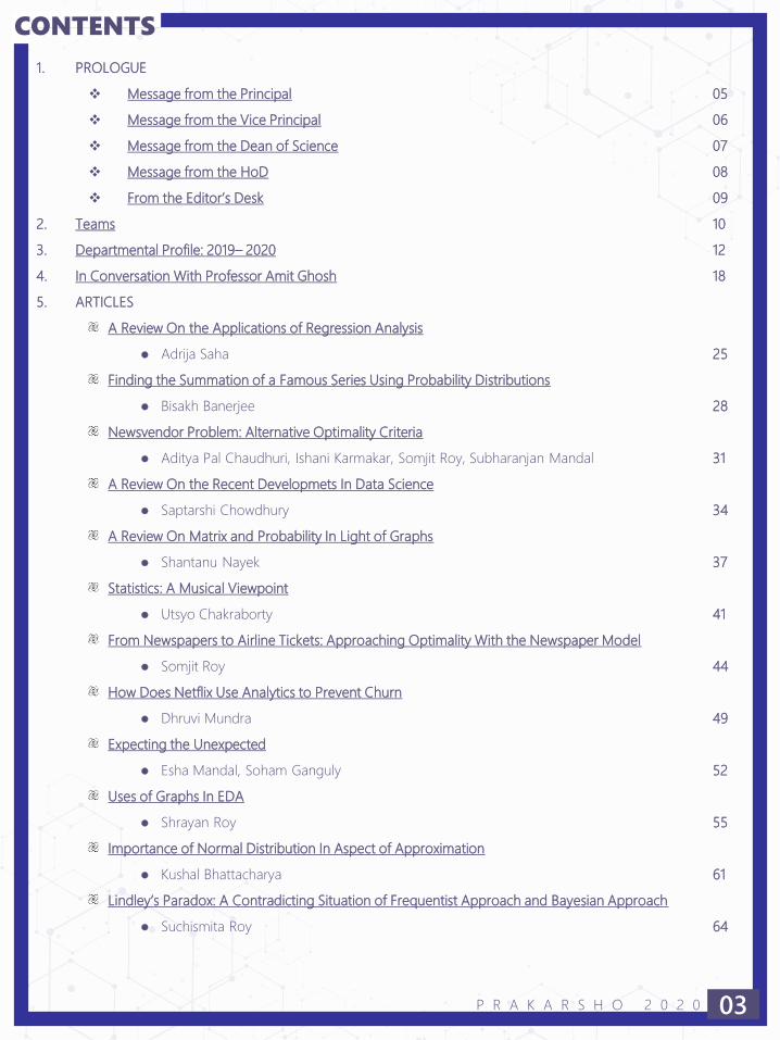
CONTENTS
1. PROLOGUE
❖ Message from the Principal 05
❖ Message from the Vice Principal 06
❖ Message from the Dean of Science 07
❖ Message from the HoD 08
❖ From the Editor’s Desk 09
2. Teams 10
3. Departmental Profile: 2019– 2020 12
4. In Conversation With Professor Amit Ghosh 18
5. ARTICLES
A Review On the Applications of Regression Analysis
● Adrija Saha 25
Finding the Summation of a Famous Series Using Probability Distributions
● Bisakh Banerjee 28
Newsvendor Problem: Alternative Optimality Criteria
● Aditya Pal Chaudhuri, Ishani Karmakar, Somjit Roy, Subharanjan Mandal 31
A Review On the Recent Developmets In Data Science
● Saptarshi Chowdhury 34
A Review On Matrix and Probability In Light of Graphs
● Shantanu Nayek 37
Statistics: A Musical Viewpoint
● Utsyo Chakraborty 41
From Newspapers to Airline Tickets: Approaching Optimality With the Newspaper Model
● Somjit Roy 44
How Does Netflix Use Analytics to Prevent Churn
● Dhruvi Mundra 49
Expecting the Unexpected
● Esha Mandal, Soham Ganguly 52
Uses of Graphs In EDA
● Shrayan Roy 55
Importance of Normal Distribution In Aspect of Approximation
● Kushal Bhattacharya 61
Lindley’s Paradox: A Contradicting Situation of Frequentist Approach and Bayesian Approach
● Suchismita Roy 64


MESSAGE
FROM THE PRINCIPALRev. Dr. Dominic Savio, SJPrincipal
St. Xavier’s College (Autonomous), Kolkata
“I am happy to note that the Department of Statistics of our college is
successfully publishing its annual departmental magazine, the 2020
edition of Prakarsho.
It is good to see the Department uphold its tradition of excellence and
distinction, which the department magazine bears testimony to. Since
its inception in 1996 the department has strived to hone new skills and
abilities. One of its striking endeavors is that of exploring the prospect
of research on the subject into which we get a tiny peek from the
articles by students in the magazine.
My hearty congratulations to the entire department, to its faculty and
students. I wish them success on their efforts in publishing this issue of
the magazine and many more subsequent ones in the years to come.
God bless you all! Nihil Ultra!”
05P R A K A R S H O 2 0 2 0
REV. DR. DOMINIC SAVIO, SJ
PRINCIPAL
MESSAGE
FROM THE VICE PRINCIPALProf. Bertram da SilvaVice Principal
St. Xavier’s College (Autonomous), Kolkata
“Once again it is time to congratulate the faculty and students of the
Department of Statistics for publishing the latest edition of the
departmental magazine, Prakarsho 2020.
The magazine is tangible proof of the department’s pursuit of academic
excellence and creativity. The magazine is an incentive for research and
analysis, and by providing a space for publishing work, it helps train
students in the rigours and protocols of academic writing. This has the
proper merit of preparing them for the challenges and opportunities of
post-graduate study.
If the Department of Statistics has an exceptional reputation and record
of academic excellence, it is due in no short measure to its commitment
to academic excellence. Prakarsho 2020 is evidence of that
commitment.”
06P R A K A R S H O 2 0 2 0
PROF. BERTRAM DA SILVA
VICE PRINCIPAL

MESSAGE
FROM THE DEAN OF SCIENCEDr. Tapati DuttaDean of Science
St. Xavier’s College (Autonomous), Kolkata
“It is a pleasure to know that the Department of Statistics is ready to
bring out the 2020 edition of its annual departmental magazine
Prakarsho.
The magazine and the articles within speak volumes about the
enthusiasm, motivation, and ambition of the students regarding their
field. It is refreshing to see students going beyond their curriculum to
make this happen.
I would like to congratulate the department on the success of their
current endeavour and I wish them success for their future.”
07P R A K A R S H O 2 0 2 0
DR. TAPATI DUTTA
DEAN OF SCIENCE

MESSAGE
FROM THE HEAD OF THE DEPARTMENTDr. Durba BhattacharyaHead, Department of Statistics
St. Xavier ’s College (Autonomous), Kolkata
“It instils in me a sense of immense pride and pleasure to see our
students bring out the 12th edition of our Departmental Magazine
Prakarsho. Their untiring efforts and relentless energy is indeed
praiseworthy.
I would like to extend my heartfelt gratitude to Father Principal, Vice-
Principal, Dean of Science and Dean of Arts for their perennial guidance
and encouragement. I wish to thank the Program and Publication
Committee for their continuous support.
My sincere thanks and appreciation goes to my colleagues, whose
efforts and endeavours as a team has helped us come together to
unveil yet another reflection of our department.”
08P R A K A R S H O 2 0 2 0
DR. DURBA BHATTACHARYA
HEAD, DEPARTMENT OF STATISTICS

MESSAGE
FROM THE STUDENT EDITOR’S DESK
“Before you turn over the pages, and delve into a carnival of statistical
thoughts and ideas, let us first thank the team, whose untiring effort
and enthusiasm, has led to the publication of the magazine. Prakarsho
is nothing less than a dedicated teamwork, a delightful journey with the
flair for excellence, creativity, imagination and zeal that sets a
benchmark for itself.
Prakarsho is not just a mere collection of articles; it’s that thread that
binds the Department Of Statistics. Starting from the professors, to the
various working committees namely Editorial, Publication, Designing,
Finance, and Cultural, and each & every student of the department-
there is hardly anyone who did not lend a hand in this journey.
We would also like to express our heartfelt gratitude to all the authors,
sponsors, publishing house and well-wishers for their zealous support
and co-operation.
Hence, with immense hope and pleasure, we present to you the 12th
Volume of Prakarsho.”
09P R A K A R S H O 2 0 2 0
Student Editor
Dattatreya Mitter
Associate Student Editor
Sreejit Roy
Editorial Team
10P R A K A R S H O 2 0 2 0
Students Editorial Board
Niladri Kal
Shubha Sankar Banerjee
Soumyabrata Bose
Arghamalya Biswas
Somjit Roy
Soumyadipta Ghosh
Swaagata Das
Supriyo Sarkar
Surotama Chakraborty
Advisory Board
Vice Principal, Arts and Science
Prof. Bertram da Silva
Dean of Science
Dr. Tapati Dutta
Dr. Surabhi Dasgupta
Dr. Surupa Chakraborty
Prof. Debjit Sengupta
Prof. Pallabi Ghosh
Dean of Arts
Dr. Argha Banerjee
Dr. Ayan Chandra
Dr. Durba Bhattacharya
Prof. Madhura Das Gupta
Patron
Rev. Dr. Dominic Savio, SJ

Working Committee Members
Sutirna Chakraborty
Srijit Mondal
Supratim Pal
Soham Biswas
Amrita Bhattacharjee
Rajnandini Kar
Finance Board
Srijit Mondal
Adrija Bhattacherjee
Rajnandini Kar
Mehuli Bhandari
Srija Mukhopadhyay
Tithi Sharon Sarkar
Events Team
11P R A K A R S H O 2 0 2 0
Student Covenor
Oiendrila Basak
Events Head
Archik Guha
Student Co-Convenor
Srijan Sen
Cultural Head
Rajdeep Saha

Student’s AchievementsFebruary 2019 - February 2020
6 students from the Department got selected at Indian Statistical Institute, for
pursuing M.Stat program and 11 students got selected at different IITs all over
India after qualifying the Joint Entrance Test for MSc. in Statistics.
Awards and Recognitions (3rd Year)
1. Vanshika Tantia
a) Second place in women’s double scull for 2000m and 500m in the All
India Inter University Rowing Nationals held from 24th February till 1st
March 2019 in Chandigarh.
b) Gold in women’s coxed fours in BRC Inter-college Regatta. 2.
2. Debarshi Chakraborty
a) Has won Bronze(team event)---Amephoria, Amity University
b) Gold (singles)---Xavrang, SXUK
c) Champion in XPL 2019 (Table Tennis).
d) Runner Up in Xavotsav 2020 (Table Tennis).
e) Represented North Kolkata district in Bengal State Table Tennis
Championship 2019 - won Bronze medal in team event.
f) Represented SXC Kolkata in CU Inter College Table Tennis tournament
2019- won silver medal in team event.
3. Sreeja Deb Ray
a) 1st prize in Badminton Doubles in annual sports event KHEL organized
by NCC.
Departmental Report2020
12P R A K A R S H O 2 0 2 0
4. Shibashish Mukherjee
a) All India Karate competition, 2nd
place held on July 12 2019 in New
Delhi.
5. Srijit Mondal
a) Ne8x Literature Fest- Author of
the Year 2020.
b) GFEL- World’s top 100 Education
Innovators Nominee.
Awards and Recognitions (2nd Year)
1. Ishita Pandey
a) 1st Place in Discus Throw and Triple
Jump.
b) Awarded Best Athlete in Annual
Sports 2020.
2. Soham Majumder and Tishyo Chakraborty
secured 1st place in INFINITE DIVERGENCE
in SIGMA 2019 organized by St. Xavier's
College Science Association.
3. Samiran Ghosh, Sovon Gayen and
Purnaloke Sengupta secured 2nd place in
BATTLE ROYALE in SIGMA 2019 organized
by St. Xavier's College Science Association.
4. Somjit Roy
a) Runner-up in Inter Collegiate
Cricket Tournament, Calcutta
University.
5. Supratim Pal
a) Silver in 4th Inter College Rowing
Championship 2019.
b) Represented INDIA in ARAE
Colombo 2014 and received GOLD.
6. Sabuj Ganguly secured 1st place in Creative
Writing in SRIJAN 2019.
7. Srijan Sen won the 'Author of the Week'
title in Inter College Creative Writing
Competition ― Bengali Poetry Category
by Storry Mirror.
8. Srijan Sen, Soham Majumder, Supratim Pal
and Ritoban Sen presented a paper on ‘A
Simulation Study Of Sample Size
Determination For Achieving Normality Of
Binomial Distribution’ in Indian Science
Congress 2020.
9. Srijan Sen, Soham Majumder, Supratim Pal
and Ritoban Sen presented a paper on ‘A
Simulation Study Of Sample Size
Determination For Achieving Normality Of
Binomial Distribution’ in Indian Science
Congress 2020.
10. Soham Biswas, Ishani Karmakar, Srijan Sen
and Brishti Sarkar presented a paper on ‘A
Simulation Study Of Sample Size
Determination For Achieving Normality Of
Beta Distribution’ in Indian Science
Congress 2020.
11. Soham Biswas, Tishyo Chakraborty, Somjit
Roy and Arpita Saha presented a paper on
Situations of Supply in the Classical
Newsboy Problem in Indian Science
Congress 2020.
12. Ritoban Sen, Supratim Paul, Arpita Saha
and Brishti Sarkar presented a paper on
‘Newsboy Problem: Estimation of Optimal
Order Quantity’ in Indian Science Congress
2020.
13P R A K A R S H O 2 0 2 0
DEPARTMENTAL REPORT 2020
13. Soham Majumder, Tishyo Chakraborty,
Subharanjan Mondal and Aditya Paul
Chaudhuri presented a paper on
‘Reduction of Stress Induced Diabetes in
Urban Population Through Yoga - A
Statistical Approach’ in Indian Science
Congress 2020.
14. Subharanjan Mondal, Aditya Pal
Chaudhuri, Somjit Roy and Ishani Karmakar
presented a paper on ‘Newsvendor
Problem: Alternative Optimality Criteria’ in
Indian Science Congress 2020.
15. Pallavi Chakravarty, Ramyani Dutta and
Souhardya Mitra presented a paper on
‘Statistical Analysis of Antibiotic Effectivity
& Sensitivity of Urinary Tract Infruction
Causing Bacteria in Urban Population’ in
Indian Science Congress 2020.
Awards and Recognitions (1st Year)
1. Shantanu Nayek
a) Gold medal in ‘Inter Mission
Football League’.
2. Saptarshi Chowdhury
a) ’Special Mention’ award in Intra
DPS MUN in UNHRC and Third
place in ‘Regional Mathematics
Olympiad’ in Assam.
3. Soham Ganguly
a) Winner of Inter Departmental table
tennis tournament in SXC in 2019.
b) Member of the College Table Tennis
team that won Silver at the Calcutta
University Inter College Table Tennis
tournament.
c) Runner’s Up- XPL (table tennis).
d) Champion (Table Tennis)-
Bhawanipur Education Society
College Fest (Umang).
e) Champion (Table Tennis)- JDBI Fest
(Invictus).
f) Participated and completed 10Km
marathon organized by Tata Steel.
g) Participated and completed 10Km
marathon organized by IDBI
Federal Life Insurance.
h) Won Silver at East Endurance
Cycling Challenge(80Km) organized
by Cycle Network Grow.
4. Adrija Bhattacharya and Debolina
Bhattacharya Winner of ‘HRPR’ event in
Enthusia 2019 conducted by EnactusSXC.
5. Gourav Daga
a) Third place for TCS Quiz on science
and technology.
6. Rajnandini Kar
a) Third place in Inter department
table tennis tournament in SXC in
2019
b) 2nd in Inter Departmental Table
Tennis tournament.
c) 3rd in Inter Department Football
tournament.
14P R A K A R S H O 2 0 2 0
DEPARTMENTAL REPORT 2020

8. Sandip Chakraborty
a) CU Inter College Team- Silver.
b) Umang(Inter College fest at
Bhawanipur college)- Gold (team
event).
c) Xavotsav- Bronze (Singles)
d) Invictus (JD Birla Inter College fest)-
Gold (Doubles).
Participation and Certificates (3rd Year)
1. Debarshi Chakraborty
a) Represented North Kolkata district
team in West Bengal Inter district
Table Tennis championships.
b) St. Xavier ’s College Team
throughout the season.
2. Bisakh Banerjee was selected to attend a
summer camp in Mathematics in Chennai
Mathematical Institute (CMI) in June 2019
organised by National Board of Higher
Mathematics.
3. Tanuj Sur co-authored “An Innovative
Method to Calculate the Economic
Development Index of Important Cities in
West Bengal from Satellite Imagery”,
published in International Journal of
Computer Sciences and Engineering.
4. Ankita Prakash
a) One of the 120 selections in India
for the Explore ML program of
Google India.
5. Niladri Kal was selected for JBNSTS Talent
Enrichment Program from June 30th to
July 7, 2019.
6. Dattatreya Mitter, Arghyamalya Biswas,
Annesha Deb and Srijit Mondal co-
authored “URO VABNAR JONMOSTUP” a
poetry book published by Starlet
Publication.
7. Sreejit Roy got a poem published in yearly
magazine “MOITREYO MANDAS”.
8. Dattatreya Mitter got his poem published
in the book “C/O ANTORIK”.
Participation and Certificates (1st Year)
1. Rajnandini Kar
a) Certificate in Economics quiz from
SRCC.
b) Certificate in guitar from ‘Trinity
College of London’.
2. Rohit Dutta got certificate for ‘Tabla’ from
Pracheen Kala Kendra.
3. Utsyo Chakraborty got certificate for piano
from ‘Trinity College of London’.
4. Tanishi Parasramka Qualified and got a
certificate for the top 5 in Inception, the
fest by XCS.
15P R A K A R S H O 2 0 2 0
DEPARTMENTAL REPORT 2020
Placement Details
This year, a lot of students from the final year
of the department bagged lucrative
placement offers, through the SXC Placement
Cell.
1. Archik Guha and Ayushi Biyani were
offered the post of Associate Analyst at
Deloitte USI.
2. Nandini Agrawal was offered the post of
Tax Analyst at Ernst & Young Global
Delivery Services.
Departmental Activities
Coverage of Epsilon Delta, 2019
On 20th March, 2019, Department of Statistics,
St. Xavier ’s College (Autonomous), Kolkata,
embarked upon an era of success and
achievements as it was glorious to behold the
third edition of the annual departmental event
“Epsilon Delta”. The inaugural ceremony being
hosted by respected Principal and Rector Rev.
Fr. Dr. Dominic Savio, S.J. and other dignitaries
of the college administration, the luster of the
event reached it’s brilliance with the release of
the 11th volume of the departmental magazine
“Prakarsho”, which imbibed the ideas of Prof.
Sugata Sen Roy of Department of Statistics,
University of Calcutta and Prof. Bimal Kumar
Roy , former director of Indian Statistical
Institute (ISI), Kolkata. The magazine also
showcased the statistical as well as academic
approaches of the young minds that is the
students of the department itself from 1st, 2nd
and 3rd year in the form of articles. The
seminar was marked by the great presence of
Prof. Bikas Kumar Sinha , ISI Kolkata who
3. Sayak Giri was offered the post of Trainee
Data Science Executive at Spring & River.
4. Sutirna Chakraborty was offered the post
of Associate Analyst at Swiss Re.
introduced and conveyed some well known
and important aspects Departmental
Activities: of Game Theory. Along with Prof.
Sinha, the occasion was enlightened by Prof.
Gaurangadeb Chattopadhyay of University of
Calcutta. Not only the seminar witnessed great
professors and dignitaries but also provided
ample opportunities to the students of
Statistics Department and other departments
of the college as well, as students from other
colleges, proved their academic excellence
and diversity through events like “Proectura”
(Paper Presentation), “Xposure” (Online
Photography) and “Inquisitive” (Quiz
competition). The daylong seminar earning
great appreciation and engraving the
memories created within the faculty members
and students of Statistics concluded with a
cultural programme performed by the
students of the department itself.
16P R A K A R S H O 2 0 2 0
DEPARTMENTAL REPORT 2020
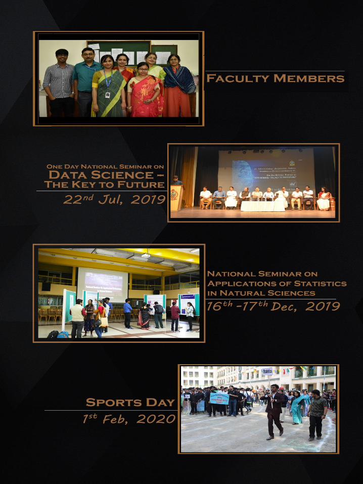
Data Science Seminar, July 2019
One day National Seminar on “ Data Science-
The key to Future”, was jointly organized by
the Departments of Computer Science and
Statistics, in collaboration with The Data
Science Foundation on 22nd July 2019, at Fr.
Depelchin Auditorium. Pro-Vice-Chancellor for
Academic Affairs of University of Calcutta, Prof.
Asis Kr Chattopadhyay was the Chief Guest
and Dean of Faculty Councils for PG studies in
Engineering and Technology, University of
Calcutta, Prof. Amlan Chakraborty was the
Guest of Honour. Mr. Kaustav Majumdar and
Mr. Gautam Banerjee, from Data Science
foundation were the first two speakers of the
day. Prof. Sourabh Bhattacharya from Indian
Statistical Institute and Mr. Sanjoy Karmakar
from IBM were speakers for the third and
fourth session respectively. More than 400
students from our college, along with teachers
and professionals from Other Colleges/
Universities attended the seminar.
Two Days National Seminar on Applications of
Statistics in Natural Sciences, December 2019
Two days National Seminar on "Applications of
Statistics in Natural Sciences", was jointly
organized by the Departments of Statistics
and Physics in collaboration with IUCAA
Centre for Astronomy Research and
Development (ICARD), Kolkata on December
16th and 17th,2019. Pro-Vice-Chancellor for
Academic Affairs of University of Calcutta, Prof.
Asis Kr Chattopadhyay was the Chief Guest for
the seminar. Oraland poster presentation
showcasing the research of College and
University teachers and Research Scholars
from different fields of Natural Sciences were
carried on both the days. In total 15 oral
presentations and 12 posters were presented.
Best oral presentation award was achieved by
Debashish Chatterjee of ISI, Somsubhra Ghosh
of IACS, Kolkata and Sreetama Das Choudhary.
Best Poster award was won by Avinanda
Chakraborty of Prsidency University. In
addition, the seminar also had specialized
sessions by invited eminent speakers like Prof.
Ayanendranath Basu, Prof. Saurabh Ghosh and
Prof. Supratik Pal from Indian Statistical
Institute and Prof. Rajesh Kumble Naik from
IISER Kolkata. More than 100 teachers and
research scholars from St. Xavier ’s College,
Kolkata and Colleges/Universities from other
states attended the seminar.
17P R A K A R S H O 2 0 2 0
DEPARTMENTAL REPORT 2020
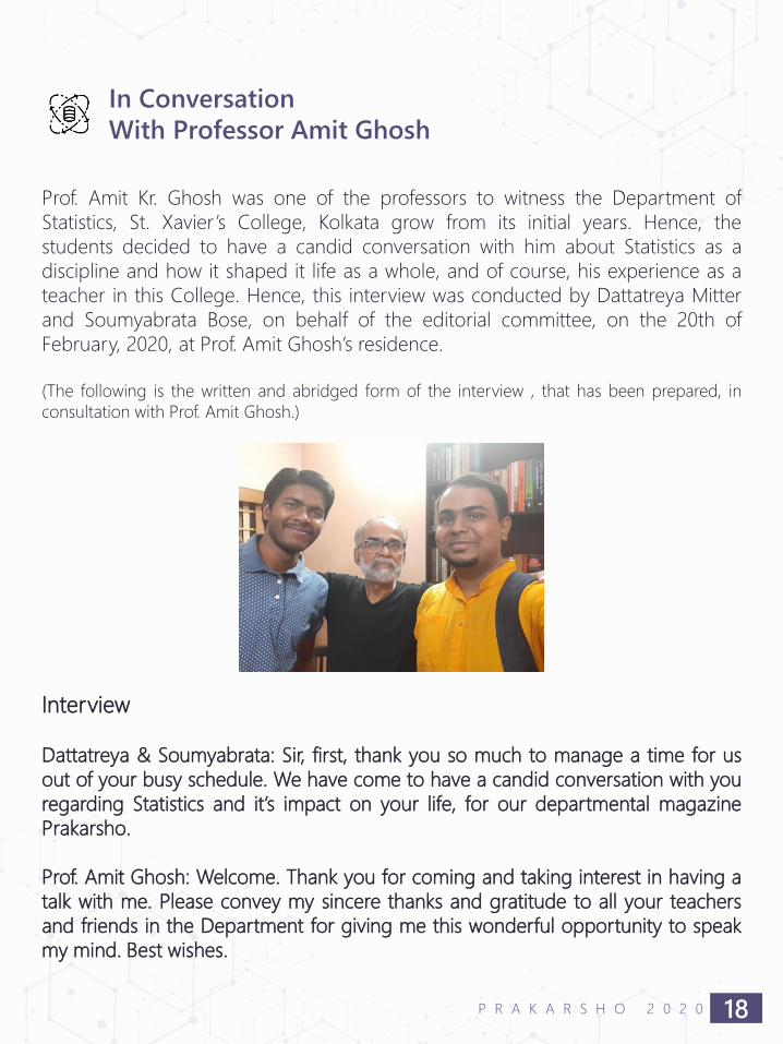
Prof. Amit Kr. Ghosh was one of the professors to witness the Department of
Statistics, St. Xavier ’s College, Kolkata grow from its initial years. Hence, the
students decided to have a candid conversation with him about Statistics as a
discipline and how it shaped it life as a whole, and of course, his experience as a
teacher in this College. Hence, this interview was conducted by Dattatreya Mitter
and Soumyabrata Bose, on behalf of the editorial committee, on the 20th of
February, 2020, at Prof. Amit Ghosh’s residence.
(The following is the written and abridged form of the interview , that has been prepared, in
consultation with Prof. Amit Ghosh.)
Interview
Dattatreya & Soumyabrata: Sir, first, thank you so much to manage a time for us
out of your busy schedule. We have come to have a candid conversation with you
regarding Statistics and it’s impact on your life, for our departmental magazine
Prakarsho.
Prof. Amit Ghosh: Welcome. Thank you for coming and taking interest in having a
talk with me. Please convey my sincere thanks and gratitude to all your teachers
and friends in the Department for giving me this wonderful opportunity to speak
my mind. Best wishes.
In Conversation
With Professor Amit Ghosh
18P R A K A R S H O 2 0 2 0

Q1. Sir, please share something about your
childhood and school days.
I was born & brought up in a large joint family
comprising of people of three generations
living together in an ancestral house located in
the heart of North Calcutta. Our childhood
and adolescence was enwrapped in a Hindu
Bengali middle class social milieu with all its
characteristic ethos, customs, dreams and
despair. The rat-race to grab a creamy slice of
‘success’ at the cost of all other moral and
social values did not engulf the mindscape of
our parents and teachers. We didn’t
experience much tension & anxiety about the
prospects of our future. Rather we enjoyed
enough freedom of thought and many poised
moments to stand & stare.
I was a student of Metropolitan
Institution(Main) in a close proximity to our
residence. Its founder-headmaster was
Iswarchandra Vidyasagar and it was a part of
the adjacent Vidyasagar College as we find in
the case of our SXCS and SXC today. It was a
traditional Bengali medium school that was
truly a ‘neighbourhood’ school bonding
teachers and generations of students & their
parents living around its sacrosanct building. I
wonder today how we were blessed with a
bunch of dedicated & distinguished teachers
who as true disciples of Iswarchandra
preached by their deeds the lofty idea of ‘plain
living & high thinking.’ They tried their best to
imbue our mind with all kinds of moral values,
patriotism, thirst for knowledge and above all
an aspiration to serve the country & its
people. Till this day I recall them with profound
regard &tears of gratitude.
Ours was system of school living examination
at the end of class 11 and the syllabi were
composed of all those from class 9 to 11.In our
Metropolitan school, we had a privilege of
getting routine lectures on some portions of
our syllabi of Physics, Chemistry, Mathematics
& English by the renowned professors of
Vidyasagar College, City college & Scottish
Church College which were some of the
premier colleges in North Calcutta of our time.
Q2. Sir, how were your college days?
After my H.S. Exam I took admission in The
Presidency College which was at a stone’s
through from our house. I spent my days there
in the late 60’s & early 70’s of the last century.
That was a great time for me to learn. The
whole world was witnessing a stormy time of
deep economic crisis, imperialist aggressions,
peasant revolts, workers strikes and student
upsurges. This turbulent time impacted our life
in the college campus. That very ambience
helped us to grow as adult citizens responsive
to the issues & questions about the age-old
traditions, social injustices and people’s
struggle against economic exploitation and
political repression. All these left an indelible
imprint on our young minds.
Q3. Sir, why did you choose Statistics as your
Honours subject after the completion of HS
Examination?
To tell you the truth, in those days people
around me had little idea about the exact
nature and scope of Statistics. The teachers of
our school inculcated in me a keen interest in
Mathematics. Also, I and some of my friends
were inspired by Prof Prasanta Chandra
Mahalanobis’ vision of Statistics as a novel
mathematical technology of the 20th century
for the development of science and society.
We took much interest in the articles
19P R A K A R S H O 2 0 2 0
IN CONVERSATION WITH PROFESSOR AMIT GHOSH
on this subject published in ‘Jnan O Bijnan’, a
popular monthly Bengali magazine for school
students of our time. However, as I go down
the memory lane to relook into the choice of
the subject, it now seems to me that the key
issue was something else. The unknowns
rather than the knowns beaconed the young
minds.
Q4. Sir, tell us a few words about your
experiences in the Statistics Department of the
Presidency College.
In fine, that was great. It had the distinction of
introducing Statistics as a Major subject in the
undergraduate curriculum in 1944, the first of
this kind in India. In our time we were
privileged to have one of the star faculties of
the college: Prof A Bhattacharya, Prof A M
Goon, Prof M K Gupta, Prof B Dasgupta, Prof B
Das, Prof D Basu and Prof A S Nag. It was a
bunch of most distinguished and dedicated
scholars and teachers that one could imagine!
Prof A Bhattacharya, as you know, is famous
for his enunciation of ‘Bhattacharya’s
Inequalities’ in statistical inference that provide
more stringent inequalities than that by ‘Rao
Cramer Inequality’. We witnessed the evolution
of the 3rd revised & enlarged edition of
‘Fundamentals’ and the 1st edition of
‘Outlines’, two universally acclaimed text books
for the undergraduate Statistics as a Major,
almost chalked out by the legendary trio
Professors Goon
Gupta-Dasgupta on the sliding black boards in
our Honours classes. The academic
atmosphere in the Department was conducive
to a meaningful student-teacher interaction.
The average size of the Statistics Honours
classes over the years never exceeded 15. The
entire Faculty was easily accessible to the
students from morning to late evening hours
notwithstanding the regular turmoil in the
college campus. The diversity of life in the
campus made Presidency College a vibrant
centre of higher education in our time.
In this connection, it may be mentioned that
Prof A M Goon and Prof A S Nag worked for
many years as Guest Professors in our St.
Xavier ’s College after their retirements from
The Presidency.
Q5. Sir, what kinds of text books did you use
to manage your study of the Statistics
Honours papers? Do you think the ‘core’ of it
as presently taught is significantly different
from that of your time?
In our time no text books were easily available
to the students of our country that could do
justice to the standard of the CU Statistics
Honours syllabus. Most of the available books
were either too advanced and/or difficult or
too simple or terse to satisfy the real needs of
the students. We had to fall back upon 2
volumes of ‘Fundamentals’ and the rigorous
lecture notes delivered by our teachers. These
sources were thinly supplemented by books
from the college/department library such as:
• ‘Statistical Methods’ by Mills
• ‘Introduction to the theory of Statistcs’ by
Yule & Kendal
for statistical methods;
• ‘Introduction to Mathematical Statistcs’ by
Hogg & Craig
• ‘Advanced theory of Statistics’ by Kendal &
Stuart
for statistical inference;
• ‘Introduction to Mathematical Probability’
by Uspensky
• ‘Introduction to modern Probability Theoy
& its applications’ by Feller
for probability theory;
20P R A K A R S H O 2 0 2 0
IN CONVERSATION WITH PROFESSOR AMIT GHOSH
• ‘Introduction to linear statistical models’ by
Graybill
• ‘Design & analysis of experiments’ by
Kempthorne
for ANOVA & DOE;
• Algebra’ by Ferrar
• ’Finite Difference’ by Freeman
• ’Numerical Analysis’ by Scarborough
• ’Mathematical Methods’ by Courant
for mathematical methods in the Honours
course;
• ‘Sample Survey: Theory & Methods’ by
Murthy
for sampling techniques, etc.
For applied statistics topics and Indian official
statistical system we had no standard text
books/manuals other than the Volume2 of
‘Fundamentals’ though Spigelman’s
‘Introduction to Demography’ and ‘Applied
General Statistics’ by Croxton & Cowden were
available on the book shelves of the college
library. Most of the books I have just
mentioned are not in vogue now except
Feller ’s elegant and all-time great texts on
probability theory. Also, the book by Hogg &
Craig has proved its worth over time as a very
useful text book with proper rigour and are
still in use.
As to the 2nd part of your question I can say
that the ‘core’ is not radically different today
from that of our time though the syllabi have
been undergoing a lot of notable changes
since 1990’s, first in the CU and then in the
autonomous SXC.A bulk of the algebra of
determinants, calculus of finite differences and
numerical analysis was dropped from the
syllabus of mathematical methods for Statistics
and was replaced by a considerable amount of
real analysis and linear algebra. In statistical
theory, Pearsonian System of curves and
Edgeworth series expansions are no longer
taught. Various kinds of abridged life tables in
Demography, changing seasonal indices
&periodogram analysis in Time Series, Dodge-
Romig sampling plans in SQC and some other
non-core materials have been removed from
the old syllabi.
Q6. Sir, how did you manage the complicated
and heavy numerical computations in your
Statistics Practical classes without the tools of
coding, softwares and computers that we are
now used to?
Definitely, you are much privileged in a
modern statistical computing environment.
Our environment will appear to you as rather
antique. We had to use old type-writer like
‘FACIT’ machines for arithmetical operations;
‘Barlow Tables’ for roots/powers/reciprocals of
numbers; ‘Chamber ’s Seven-figure Log Tables;
‘Biometrica Tables’ by Pearson Heartley/
‘Fisher-Yates Tables’ for parametric statistical
inference and ‘Owen’s Tables’ for non-
parametric inference. We had to use Squared
papers along with Graph-papers for numerical
computations, tabulations & diagrammatic
representations, and all such jobs were to be
done with a pencil. I do not hesitate to say
that 90% of our Practical class hours were
spent in the management of numerical
computations on readymade stale data,
leaving little time for us to explore live data
and learn therefrom. The only positive quality
that such a practice imparted to us was a skill
that could make efficient ‘algorithms’ for
elaborate numerical computations. I sincerely
believe, your statistical intuitions & skills would
thrive in a much better mode in your modern
computing environment along with your easy
access to Internet resources.
21P R A K A R S H O 2 0 2 0
IN CONVERSATION WITH PROFESSOR AMIT GHOSH
Q7. Sir, how would you like to appreciate
today the under-graduate teaching-learning
process of your time?
First: that was definitely a teacher-centric
process. Lectures by teachers and notes taken
down by students passively were the only two
components that made the process. No other
modes were seriously explored in those days.
Second: there was an inherent ‘bias’ towards
‘theory’ in one sense. As Statistics is a
common research methodology for scientific
inquiries cutting across various disciplines, its
structural features bear the hallmarks of the
said methodology, i.e. quires, plausible
hypotheses, relevant data, information
measured and inductive verifications, all
carried out in an unbroken chain that repeats
and expands. This continuum is known in
modern science as ‘Hypothetico-Deductive-
Inductive’ method. We had given much
emphasis on the deductive manipulations of
‘measures’ and rigorous mathematical
treatments of ‘methods’ in isolation from
actual data and real questions to be resolved,
at the cost of ‘exploration’ of data, ‘heuristic’
arguments and inductive modelling. I strongly
believe that with the advancement of Statistics
as a distinct discipline and its computing
environment, we had, in this regard, made a
lot of progress in the recent past; and I am
sure we would be more able, over time, to
mend the process and transcend the
limitations in the interest of students.
Q8. Sir, please tell us in a few words your
experiences in Post Graduate classes?
I obtained my Master ’s degree from the CU.
The Statistics Department was situated on the
5 th floor of a modern multi-storey building at
Ballygunge Circular Road. The department
was established in 1941 as the first of this kind
in India. When we entered this department its
faculty had a very rich profile made by some
of the most eminent scholars and teachers of
that time. To mention a few names: Prof H K
Nandi, Prof P k Banerji, Prof B Adhikary, Prof S
K Chatterji, Prof S P Mukhopadhyay, Prof A
chaudhury, Prof B K Sinha. They elevated the
department to the most respectable national
level through their research work in the field of
statistical theory & methods and regular
rigorous teaching in the Post Graduate classes.
Prof S P Mukhopadhyay introduced
Operations Research in the conventional
curriculum of Statistics and taught the same as
a special paper offered to us. He did
pioneering works in Industrial Quality
Management and extended their lessons to
enlighten the industrial managements in India
and abroad.
As to the availability of text books, the
mainstream of teaching-learning process and
the routine practices in practical classes, I think
today that no new window was really opened
up after our under graduate days. The deep
ruts of the tradition remained unaltered.
Q9. Sir, please tell us something about the
scopes for learning Statistics and securing
professional jobs in your time. Do you think
that the scenario is different at present?
Definitely, the present scenario is quite
different in multiple respects. In our days the
number of educational institutions offering UG
and/or PG programmes were very limited in
number. In our State only 3 colleges under CU,
i.e., Presidency, Asutosh, Narendrapur RKM
offered UG programmes and ISI, both UG
&PG. Outside the State, The University of Pune
also offered such programmes. There was
22P R A K A R S H O 2 0 2 0
IN CONVERSATION WITH PROFESSOR AMIT GHOSH
paucity of research fellowships with a
reasonable stipend in our country and abroad.
The opportunity for doing Master’s degree
outside the country was also thin. In the
academic arena of our country the faculties of
science & technology stood far away from
modern interdisciplinary research activities.
There were no national or multinational
corporations with their Analytic wings on our
soil seeking professional statisticians for
research & development. The Indian Statistical
services (ISS) was the major service provider
for professional jobs through its public
examinations. It recruited statisticians for the
Indian Statistical Offices. Even in this field the
recruitments were neither frequent nor large in
numbers. Also, the pay packet and facilities
were not so lucrative. Extensive changes have
taken place in all these spheres widening the
scopes for higher learning and ushering in
new job prospects. Even the Government of
India has established a separate Ministry Of
Statistics & Programme Implementation
(MOSPI) and a Central Statistical Commission
(CSC).It has also extended and upgraded the
ISS.
It is not difficult to see why and how such
changes have taken place. You are living in an
age of digitized information and Statistics is
the key technology for the most efficient
navigation through the oceans of such
information. Brace up for a voyage.
Q10. Sir, tell us in brief how do you take on the
recent trends and prospects of Statistics.
The 21st century, i.e., your millennium, is
witnessing an enormous ‘explosion’ of
information due to an all pervasive digital
revolution. The enormity of its impact induces
‘paradigm shift’ in almost every domain of our
science & technology. The conventional
frontiers of the distinct domains are
intertwining giving rise to redefinitions and
new contours. Statistics is no exception. In the
interdisciplinary fields of Data Science or Big
Data Analytics, diverse disciplines such as
Mathematics,
Statistics, Machine Learning & Deep Learning
Algorithms are mingled reinforcing one
another. It leads to more efficient management
& manipulation of data of enormous volume,
variety and velocity. In this connection, I may
also mention that Bayesian Statistical Inference
is reinventing itself extending the horizon of
classical inductive inference.
Q11. Sir, how do you appreciate our Choice
Based Credit System (CBCS)?
CBCS is definitely a student-centric new
curriculum as compared to our old annual
system based on rigid patterns and marks. It
offers multiple benefits to students according
to their needs and inclinations. Of course,
when I make this comment, I assume that
infrastructure, faculty strength and faculty
upskilling are up to the mark. Moreover, its
introduction and success call for much
attention and vetting in the following three
areas
1) Framing and revision of syllabi from the
perspective of their ‘dynamic core’ rather
than their ‘additive or cumulative’ growth.
2) A student-centric and innovative teaching-
learning mode.
3) Compatibility of the ‘volume’ and the
‘difficulty level’ of the syllabi with a
rationally worked out ‘average study-
hours’ (class & self-study) for a student
per semester. This is absolutely necessary
for proper assimilation of the lessons of
each semester syllabi and their retention
over semesters.
23P R A K A R S H O 2 0 2 0
IN CONVERSATION WITH PROFESSOR AMIT GHOSH

Q12. Sir, we have heard from our professors
and ex-students that you are a great teacher;
we would like to know how did you get
interested in teaching.
I shall answer your question but with a caveat.
I am not a great teacher. I am miles away from
any kind of greatness. What one can say, I
tried sincerely to deliver my best. That is it. No
more and no less. I was impressed and
inspired by some great teachers whom I came
across in my life and adored much. I tried to
imbibe their spirit and in my humble capacity
thought to tread on their heels. When I
completed my Master ’s degree, I realized that
the immense scope of the subject was not fully
explored in our country. We need more
research & training institutes, more scholars
and teachers to carry the task forward. We
need more skilled hands & brains. This vision
charted the roadmap. The rest were intimate
details of a personal life.
Q13. Sir, you had spent a long time in our St.
Xavier's College. How were the days?
In fine, wonderful. I have no hesitation to say
that I spent some great moments with my
students and colleagues in the Department
and the College at large. I shall cherish the
memories through the rest of my life.
St. Xavier ’s always stands for something Big. It
upholds plurality and secularism in the Indian
culture. Students joined this college and built
bonds with one another cutting across the
boundaries of regions, languages, religions,
castes & creeds. I learnt a great lesson from
them. The Department & SXC was my second
home. But I knew it was so to the students of
our Department also. I still remember the day
when some of them entered the department
room on the top of the college building and
proposed their teachers without hesitation that
they had planned to publish an annual
departmental academic magazine on a
regular basis and they had also thought a
name for it: Prakarsho. That was the beginning
of a journey.
Q14. Sir, lastly, what are your advices to
students like us?
See, I believe, I can’t advise you. I can only
share my experiences and thoughts with you
so that you can judge and reach somewhere.
Here some of my stray thoughts for you.
Preparations for a war to win and those for
battles to fight through, though interwoven,
are distinct. To strike a balance between these
two ends is the key to success…
Stay connected with people around you. Make
bonds with trust and compassion…
Accept diversity around you. Get ready to
accept differences.
Dare to know. Dare to learn. Dare to discover
your inner strengths and weaknesses. And in a
fast changing world, also dare to unlearn to
remake yourself…
Dare to dream. Dare to pursue your dreams
with passion. You can give your best to others
only when you love what you do. Always
remain true to yourself…
Lastly, I would like to share with you a few lines
from the great Arabian artist-philosopher
Kahlil Gibran:
“Your daily life is your temple and your
religion. Whenever you enter it take with
you your all.”
Dattatreya & Soumyabrata: Thank you, Sir.
24P R A K A R S H O 2 0 2 0
IN CONVERSATION WITH PROFESSOR AMIT GHOSH
Adrija Saha1st year, Department of Statistics
Regression analysis is a statistical process to find out the relationship between
some factors of interest in various purposes. It helps us to answer many questions
like: Which factors have the greatest impact? Which factors can be ignored? How
are those factors interrelated with each other? And, the most importantly, how
certain are we about those factors at all?
In regression analysis, those factors are referred to as variables. These variables are
classified into two types-
1. Dependent variable — the main factor that we are trying to predict,
2.Independent variables — the factors that we suspect to have an impact on our
dependent variable.
Now in our discussion, we are not going to discuss much about how to draw a
regression line, why it is called the ‘ Best explanation of the relationship between
the independent and dependent variable’ and all, but we are going to discuss the
real life fields in which Regression Analysis has a vast impact.
Regression Analysis in Business Forecasting:
Predictive Analysis is the most prominent application of regression analysis in
business. It is based on forecasting business opportunities and future risks.
Demand analysis deals with prediction of the demands of a certain product.
Regression analysis is a process that is heavily relied on by the Insurance
Companies to estimate the credit standing of policyholders.
Regression Analysis also increases operation efficiency in Business. For example,
using Regression Analysis, a factory manager can understand the relation between
productivity of certain product and other factors and improve the product’s
demands in market.
A Review On the
Applications of Regression Analysis
25P R A K A R S H O 2 0 2 0
Regression analysis provides a scientific view
to various business managements by reducing
huge amount of raw data into information that
is actually required, that is how regression
analysis leads the way to more perfect
decisions. This tool is used to test a hypothesis
before diving into implementation. Regression
analysis can prevent mistakes also.
Regression analysis also may uncover some
previously unnoticed patterns while finding a
relationship between different variables. For
example, it may uncover the fact that the
demand of specified product is usually
increased in a particular season of the year,
that was may not be noticed beforehand.
Regression Analysis in Machine Learning
Regression analysis helps to prepare schemes
for given situations well in advance and then
analyze its probable outcomes. As machine
learning is based on predictions, Regression
Analysis helps it in a grand way. The actionable
information that comes from Regression
Analysis helps companies to make their
strategies.
One of the biggest advantage of using Linear
regression model is to forecast trends, patterns
and making useful decisions in Machine
Learning. Moreover, these decisions can be
used further in Machine Learning. Its accuracy
level is high, efficient enough and fast.
Regression Analysis in Finance
Multiple Regression Analysis is preferable to
forecast financial statements for a company. It
is usually for determining the changes in
certain assumptions of business that will
impact in future. For example, the correlation
between the number of employees employed
by a company, the number of branches they
have and the revenue of the business, may be
very high.
Regression Analysis in Biological Experiments
There are several examples in biological
experimentation where Regression Analysis is
used.
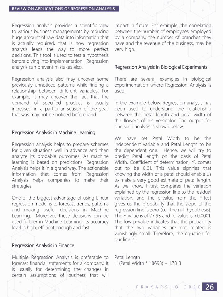
In the example below, Regression analysis has
been used to understand the relationship
between the petal length and petal width of
the flowers of Iris versicolor. The output for
one such analysis is shown below.
We have set Petal Width to be the
independent variable and Petal Length to be
the dependent one. Hence, we will try to
predict Petal length on the basis of Petal
Width. Coefficient of determination, r2, comes
out to be 0.61. This value signifies that
knowing the width of a petal should enable us
to make a very good estimate of petal length.
As we know, F-test compares the variation
explained by the regression line to the residual
variation, and the p-value from the F-test
gives us the probability that the slope of the
regression line is zero (i.e., the null hypothesis).
The F-value is of 77.93 and p-value is <0.0001.
The low p-value indicates that the probability
that the two variables are not related is
vanishingly small. Therefore, the equation for
our line is:
Petal Length
= (Petal Width * 1.8693) + 1.7813
26P R A K A R S H O 2 0 2 0
REVIEW ON APPLICATIONS OF REGRESSION ANALYSIS
Regression Analysis in Agriculture
In this field, the variables considered for
Regression analysis are Annual Rainfall (AR),
Area under Cultivation (AUC), Food Price
Index (FPI). Here, crop yield is a response
variable which depends on all these ecological
factors. There are many more factors like
Minimum Support Price (MSP), Soil
Parameters, Weather Conditions, etc. that can
affect the production of various crops and by
using techniques like data mining to analyze
the factors influencing the yield the research
work can be extended.
Regression Analysis in Artificial Neural
Engineering
The artificial neural engineering models were
built to forecast shelf life of instant coffee drink
like regression models. Both the models were
compared with each other. The investigation
shows that multiple linear regression model
was superior over radial basis model for these
type of investigations in Artificial Neural
Engineering.
Besides all these fields, there are several other
fields where Regression Analysis plays a vital
role such as in Researches, in Chemical &
Pharmaceutical Experimentation, in
Economics, in Mechanical Engineering & many
more and that is why Regression Analysis is
necessary in Multi-Disciplinary Fields.
REFERENCES:
1. http://doi.org/10.5351/CSAM.2017.24.4.339
2. Montgomery, Douglas, Peck, E. A., Vining, G. G.,
Introduction to Linear Regression Analysis, Wiley.
3. Hastie, Trevor, Tibshirani, Robert, Friedman,
Jerome, The Elements of Statistical Learning,
Springer.
27P R A K A R S H O 2 0 2 0
REVIEW ON APPLICATIONS OF REGRESSION ANALYSIS
Bisakh Banerjee3rd year, Department of Statistics
It remained an ‘Open Problem’ to evaluate the summation σ𝑛=1∞ 1
𝑛2, for almost 90
years. This problem is also known as ‘Basel Problem’ and Euler was the first person
to provide a complete solution of this problem. But people always looked for new,
interesting and enlightening approaches to solve this same problem. An
elementary but interesting approach is to use the concepts of ‘Probability
Distributions’.
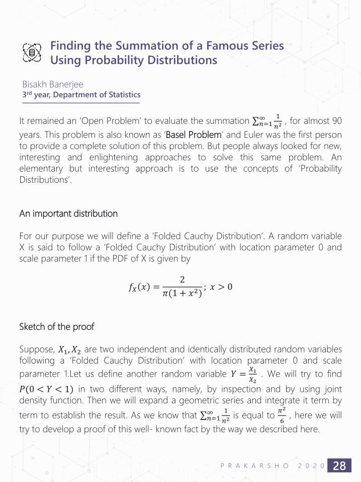
An important distribution
For our purpose we will define a ‘Folded Cauchy Distribution’. A random variable
X is said to follow a ‘Folded Cauchy Distribution’ with location parameter 0 and
scale parameter 1 if the PDF of X is given by
𝑓𝑋 𝑥 =2
𝜋(1 + 𝑥2); 𝑥 > 0
Sketch of the proof
Suppose, 𝑋1, 𝑋2 are two independent and identically distributed random variables
following a ‘Folded Cauchy Distribution’ with location parameter 0 and scale
parameter 1.Let us define another random variable 𝑌 =𝑋1
𝑋2. We will try to find
𝑃(0 < 𝑌 < 1) in two different ways, namely, by inspection and by using joint
density function. Then we will expand a geometric series and integrate it term by
term to establish the result. As we know that σ𝑛=1∞ 1
𝑛2is equal to
𝜋2
6, here we will
try to develop a proof of this well- known fact by the way we described here.
Finding the Summation of a Famous Series
Using Probability Distributions
28P R A K A R S H O 2 0 2 0
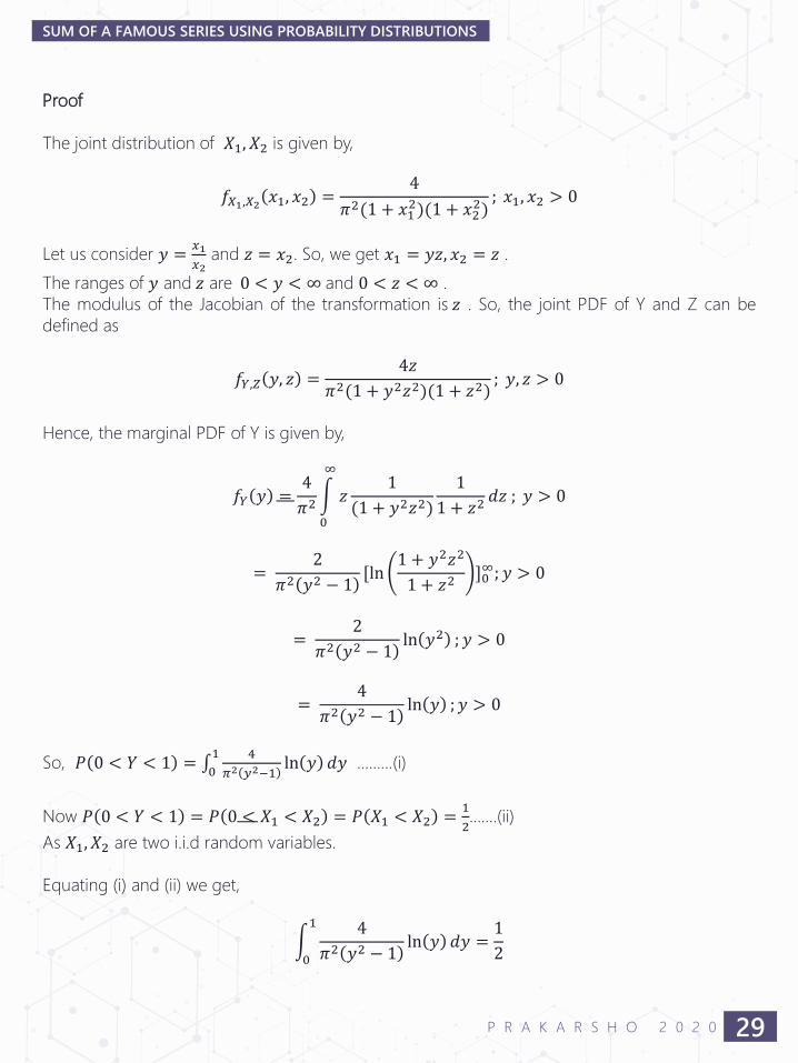
Proof
The joint distribution of 𝑋1, 𝑋2 is given by,
𝑓𝑋1,𝑋2 𝑥1, 𝑥2 =4
𝜋2(1 + 𝑥12)(1 + 𝑥2
2); 𝑥1, 𝑥2 > 0
Let us consider 𝑦 =𝑥1
𝑥2and 𝑧 = 𝑥2. So, we get 𝑥1 = 𝑦𝑧, 𝑥2 = 𝑧 .
The ranges of 𝑦 and 𝑧 are 0 < 𝑦 < ∞ and 0 < 𝑧 < ∞ .
The modulus of the Jacobian of the transformation is 𝑧 . So, the joint PDF of Y and Z can be
defined as
𝑓𝑌,𝑍 𝑦, 𝑧 =4𝑧
𝜋2(1 + 𝑦2𝑧2)(1 + 𝑧2); 𝑦, 𝑧 > 0
Hence, the marginal PDF of Y is given by,
𝑓𝑌 𝑦 =4
𝜋2න
0
∞
𝑧1
(1 + 𝑦2𝑧2)
1
1 + 𝑧2𝑑𝑧 ; 𝑦 > 0
=2
𝜋2 𝑦2 − 1[ln
1 + 𝑦2𝑧2
1 + 𝑧2]0∞; 𝑦 > 0
=2
𝜋2 𝑦2 − 1ln 𝑦2 ; 𝑦 > 0
=4
𝜋2 𝑦2 − 1ln 𝑦 ; 𝑦 > 0
So, 𝑃 0 < 𝑌 < 1 = 0
1 4
𝜋2 𝑦2−1ln 𝑦 𝑑𝑦 ………(i)
Now 𝑃 0 < 𝑌 < 1 = 𝑃 0 < 𝑋1 < 𝑋2 = 𝑃 𝑋1 < 𝑋2 =1
2…….(ii)
As 𝑋1, 𝑋2 are two i.i.d random variables.
Equating (i) and (ii) we get,
න0
1 4
𝜋2 𝑦2 − 1ln 𝑦 𝑑𝑦 =
1
2
29P R A K A R S H O 2 0 2 0
SUM OF A FAMOUS SERIES USING PROBABILITY DISTRIBUTIONS
So, 0
1 1
𝑦2−1ln 𝑦 𝑑𝑦 =
𝜋2
8………(iii)
Since, 0 < 𝑦 < 1 we will expand the series
1
𝑦2 − 1= −
𝑛=0
∞
𝑦2𝑛
By interchanging summation and integration, we get
න0
1 1
𝑦2 − 1ln 𝑦 𝑑𝑦 = −
𝑛=0
∞
න0
1
ln(𝑦)𝑦2𝑛 𝑑𝑦
Hence ,−σ𝑛=0∞
0
1ln(𝑦)𝑦2𝑛 𝑑𝑦 = σ𝑛=0
∞ 1
(2𝑛+1)2[By using integration by parts] ……………(iv)
So, combining (iii) and (iv) we have
σ𝑛=0∞ 1
(2𝑛+1)2=
𝜋2
8
Now,σ𝑛=1∞ 1
𝑛2=σ𝑛=0
∞ 1
(2𝑛+1)2+
1
4σ𝑛=1∞ 1
𝑛2
Finally , σ𝑛=1∞ 1
𝑛2=
4
3σ𝑛=0∞ 1
(2𝑛+1)2=
𝜋2
6
Hence, the proof.
Conclusion
In this way we have proposed here a ‘Probabilistic Method’ to provide an interesting solution to
the ‘Basel Problem’ and it is really surprising that we cannot give any deep insight about this
method. This solution depicts how beautiful the ‘Probabilistic Method’ can be and hence many
solved problems are still ‘Active’ in terms of giving a Probabilistic solution to the problem.
30P R A K A R S H O 2 0 2 0
SUM OF A FAMOUS SERIES USING PROBABILITY DISTRIBUTIONS
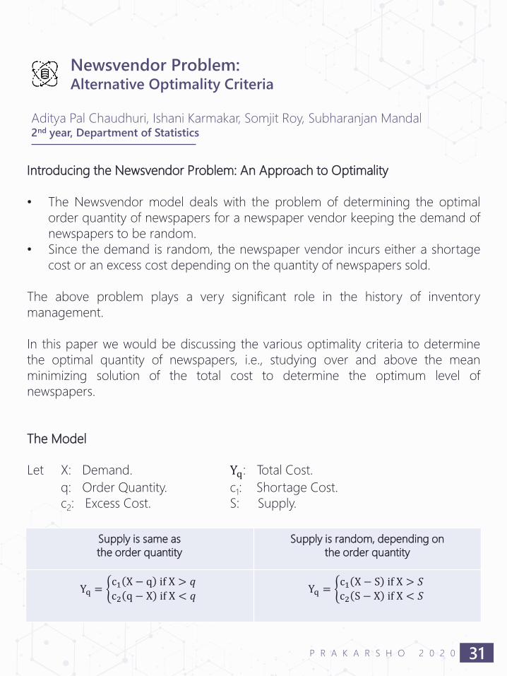
Aditya Pal Chaudhuri, Ishani Karmakar, Somjit Roy, Subharanjan Mandal2nd year, Department of Statistics
Introducing the Newsvendor Problem: An Approach to Optimality
• The Newsvendor model deals with the problem of determining the optimal
order quantity of newspapers for a newspaper vendor keeping the demand of
newspapers to be random.
• Since the demand is random, the newspaper vendor incurs either a shortage
cost or an excess cost depending on the quantity of newspapers sold.
The above problem plays a very significant role in the history of inventory
management.
In this paper we would be discussing the various optimality criteria to determine
the optimal quantity of newspapers, i.e., studying over and above the mean
minimizing solution of the total cost to determine the optimum level of
newspapers.
The Model
Let X: Demand. Yq: Total Cost.
q: Order Quantity. c1: Shortage Cost.
c2: Excess Cost. S: Supply.
Newsvendor Problem:Alternative Optimality Criteria
31P R A K A R S H O 2 0 2 0
Supply is same as
the order quantity
Supply is random, depending on
the order quantity
Yq = ቊc1 X − q if X > 𝑞
c2 q − X if X < 𝑞Yq = ቊ
c1 X − S if X > 𝑆
c2 S − X if X < 𝑆
Some Alternative Approaches
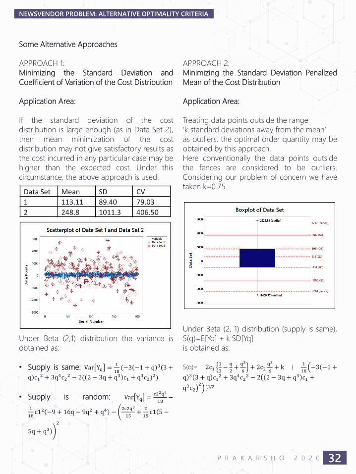
APPROACH 1:
Minimizing the Standard Deviation and
Coefficient of Variation of the Cost Distribution
Application Area:
If the standard deviation of the cost
distribution is large enough (as in Data Set 2),
then mean minimization of the cost
distribution may not give satisfactory results as
the cost incurred in any particular case may be
higher than the expected cost. Under this
circumstance, the above approach is used.
Under Beta (2,1) distribution the variance is
obtained as:
• Supply is same: Var Yq =1
18(−3 −1 + q 3(
)
3 +
q c12 + 3q4c2
2 − 2( 2 − 3q + q3 c1 + q3c2)2)
• Supply is random: Var Yq =c22q4
18−
1
18c12 −9 + 16q − 9q2 + q4 − ቆ
ቇ
2c2q3
15+
2
15c1(
)
5 −
5q + q32
APPROACH 2:
Minimizing the Standard Deviation Penalized
Mean of the Cost Distribution
Application Area:
Treating data points outside the range
‘k standard deviations away from the mean’
as outliers, the optimal order quantity may be
obtained by this approach.
Here conventionally the data points outside
the fences are considered to be outliers.
Considering our problem of concern we have
taken k=0.75.
Under Beta (2, 1) distribution (supply is same),
S(q)=E[Yq] + k SD[Yq]
is obtained as:
S(q)= 2c11
3−
q
2+
q3
6+ 2c2
q3
6+ k {
1
18ቀ
ቁ
−3(
)
−1 +
q 3 3 + q c12 + 3q4c2
2 − 2൫
൯
2 − 3q + q3 c1 +
q3c22
}1/2
32P R A K A R S H O 2 0 2 0
NEWSVENDOR PROBLEM: ALTERNATIVE OPTIMALITY CRITERIA
Data Set Mean SD CV
1 113.11 89.40 79.03
2 248.8 1011.3 406.50
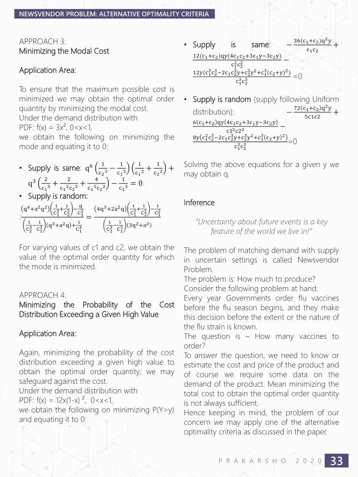
APPROACH 3:
Minimizing the Modal Cost
Application Area:
To ensure that the maximum possible cost is
minimized we may obtain the optimal order
quantity by minimizing the modal cost.
Under the demand distribution with
PDF: f(x) = 3x², 0<x<1,
we obtain the following on minimizing the
mode and equating it to 0:
• Supply is same: q61
c23 −
1
c13
1
c12 +
1
c22 +
q32
c15 +
2
c12c2
3 +4
c13c2
2 −1
c15 = 0.
• Supply is random:
:q4+a2q2
1
C12+
1
C22 −
q
C12
1
C23−
1
C13 q3+a2q +
1
C13
=4q3+2a2q
1
C12+
1
C22 −
1
C12
1
C23−
1
C13 3q2+a2
For varying values of c1 and c2, we obtain the
value of the optimal order quantity for which
the mode is minimized.
APPROACH 4:
Minimizing the Probability of the Cost
Distribution Exceeding a Given High Value
Application Area:
Again, minimizing the probability of the cost
distribution exceeding a given high value to
obtain the optimal order quantity; we may
safeguard against the cost.
Under the demand distribution with
PDF: f(x) = 12x(1-x) ², 0<x<1,
we obtain the following on minimizing P(Y>y)
and equating it to 0:
• Supply is same: −36(c1+c2)q
2y
c1c2+
12(c1+c2)qy(4c1c2+3c1y−3c2y)
c12c2
2 −
12y(c13c2
3−2c1c23y+c2
3y2+c13(c2+y)
2)
c13c2
3 =0
• Supply is random (supply following Uniform
distribution): −72 c1+c2 q2y
5c1c2+
6 c1+c2 qy 4c1c2+3c1y−3c2y
c12c22−
8y c12c2
3−2c1c23y+c2
3y2+c13 c2+y
2
c13c2
3 =0
Solving the above equations for a given y we
may obtain q.
Inference
“Uncertainty about future events is a key
feature of the world we live in!”
The problem of matching demand with supply
in uncertain settings is called Newsvendor
Problem.
The problem is: How much to produce?
Consider the following problem at hand:
Every year Governments order flu vaccines
before the flu season begins, and they make
this decision before the extent or the nature of
the flu strain is known.
The question is – How many vaccines to
order?
To answer the question, we need to know or
estimate the cost and price of the product and
of course we require some data on the
demand of the product. Mean minimizing the
total cost to obtain the optimal order quantity
is not always sufficient.
Hence keeping in mind, the problem of our
concern we may apply one of the alternative
optimality criteria as discussed in the paper.
33P R A K A R S H O 2 0 2 0
NEWSVENDOR PROBLEM: ALTERNATIVE OPTIMALITY CRITERIA
Saptarshi Chowdhury1st year, Department of Statistics
“Consumer data will be the biggest differentiator
in the next two to three years.
Whoever unlocks the realms of data and
uses it strategically will win.”- Geoffrey Moore
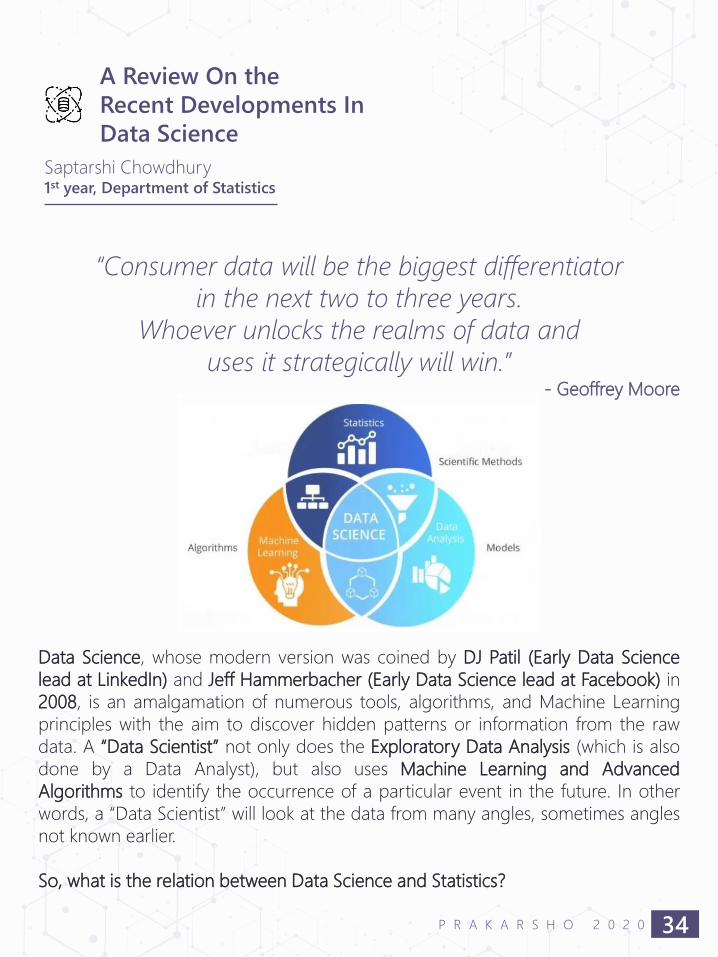
Data Science, whose modern version was coined by DJ Patil (Early Data Science
lead at LinkedIn) and Jeff Hammerbacher (Early Data Science lead at Facebook) in
2008, is an amalgamation of numerous tools, algorithms, and Machine Learning
principles with the aim to discover hidden patterns or information from the raw
data. A “Data Scientist” not only does the Exploratory Data Analysis (which is also
done by a Data Analyst), but also uses Machine Learning and Advanced
Algorithms to identify the occurrence of a particular event in the future. In other
words, a “Data Scientist” will look at the data from many angles, sometimes angles
not known earlier.
So, what is the relation between Data Science and Statistics?
A Review On the
Recent Developments In
Data Science
34P R A K A R S H O 2 0 2 0
Statistics is defined as the collection, analysis
and interpretation of numerical data. So, if
someone asks “What kind of Statistics should a
person know to become a good Data
Scientist?” The appropriate reply would be “A
person should not really worry about learning
or knowing Statistics for Data Science, but
rather just learn Statistics because it is actually
the art of unravelling the secrets hidden inside
the dataset”. Data Scientists solve problems or
help someone to take a decision, based on the
available data. They define a problem
statement (by primarily asking the right
questions) and then:
1. they collect the right kind of data to
perform their analysis.
2. they try to explore the data to see what it
tells us.
3. they employ various techniques to infer
about the data or to predict some answers
for the problem statement.
4. finally, they confirm that their
inferences/predictions are fairly accurate
(of course, by Scientific Methods!).
To perform various tasks related to a particular
query, a Data Scientist needs to keep in mind
the following algorithm:
1. He needs to have a fair idea of the domain
to which the problem statement belongs.
For example, if the Data Scientist is trying
to answer the question “Why is the GDP
Growth in India the slowest in a decade?”,
they should have a fair idea about GDP
and Economic Status of India.
2. Secondly, except for the first step, all the
other steps involve dealing with a large
amount of data in digital form. The Data
Scientist should be able to get the data,
cleanse it, read it, perform analytics, and
employ methods to arrive at answers, in a
fairly short period of time.
All the above steps are not directly performed
by a Data Scientist, but preferably from a
computer, which is, in turn, instructed by a
Data Scientist.
Moving on to the last section of the article, let
us talk about the relation between Data
Science and Big Data Analytics!
Big Data, coined by Roger Magoulas of
O’Reilly media in the year 2005, points to a
vast range of humongous data sets almost
impossible to manage and process using
traditional data management tools (which
have become too obsolete)- due to their not
only their size, but also their complexities. Big
Data has already taken the globe by storm in
the past few years, and it is of so much
significance in the present date that Geoffrey
Moore, who is an American Management
Consultant and also an Author quoted that,
“Without big data analytics, companies are
blind and deaf, wandering out into the web like
deer on a freeway”. In fact, according to New
Vantage, approximately 97.2% of
organizations, spread across the world, are
investing in Big Data and A.I.
The following points depict the relationship
between “Big Data Analytics” and “Data
Science”:
35P R A K A R S H O 2 0 2 0
REVIEW ON DEVELOPMETS IN DATA SCIENCE
1. Organizations require Big Data to improve
productivity, figure out advanced markets,
and boost competitiveness whereas Data
Science provides the algorithms or
mechanisms to understand and handle the
potential of Big Data in a timely manner.
2. Data Science provides the methods or
techniques or algorithms to decrypt or
analyze data characterized by the 3Vs
(Velocity Variety and Volume).
3. Data Science resorts the use of Machine
Learning Algorithms and Statistical
Methods to train the Computer to learn
without much programming to make
predictions from Big Data.
4. Data Science works on Big Data to derive
useful insights or information through a
predictive analysis where results or
outcomes are used to make smart
decisions.
The fact that Data Science not only benefits
the individuals pursuing it but also the society,
can be justified by the following points:
1. Redefined Customer Success: Data Science
methodologies help more customer
attributes to be utilized and put to use. For
example, data-driven companies generally
heavily depend on their audience
performance to define marketing or
advertising messaging in order to
maximize results.
2. Numerous Sectors: In case of Agriculture
Sector, according to Matthews 2019, Data
Science is completely changing the way
farmers and agricultural professionals have
been making decisions which can be
justified by the fact that farmers, these
days, utilize this technology to decide on
the amount of fertilizer, water, and other
inputs that are necessary and sufficient to
grow the best crop. Similarly, in case of
Journalism, “Data-Driven Journalism” is
considered one of the major benefits of
Data Science as it heavily motivates the
jobs of Journalists and the entire workflow
is being driven by data. Last but not the
least, Data Science benefits the Education
Sector, Airline Industry, Image and Speech
Recognition, Healthcare Industry etc.
Today, Data Science directly or indirectly
becomes a part of our daily life! Data Science
has completely transformed the way we see
Data, and has already started transforming the
global business landscape and it will keep
doing so in a much bigger aspect in the
future!
Stay tuned to deal with some “big” changes
coming up!
REFERENCES:
1. “7 Surprising Data Science Benefits” published on
Magnimind Academy on May 3, 2019.
2. “Benefits of Data Science Training” authored by
ALVERA Anto on Apr. 09, 2019.
3. “Statistics for Data Science” written by Anand
Venkatraman on June 29, 2019.
4. “The Evolution of Big data as a Research and
Scientific Topic: Overview of the Literature”
authored by Gali Halevi (MLS, PhD) and Dr. Henk F.
Moed on Sep. 2012.
5. “Is the economy in really bad shape?” by Vikas
Dhoot on Dec. 29, 2019.
6. EDUCBA Article on “Big Data vs data Science- How
are they different?”.
7. “Data Science in Agriculture” written by Abhisek
Gautam on Oct. 13, 2019.
36P R A K A R S H O 2 0 2 0
REVIEW ON DEVELOPMETS IN DATA SCIENCE
Shantanu Nayek, Sweata Majumder1st year, Department of Statistics
The concept of graphical representation is quite interesting to deal with. It is more
interesting when we think of a matrix to be represented graphically. Let’s have a
glance over it:
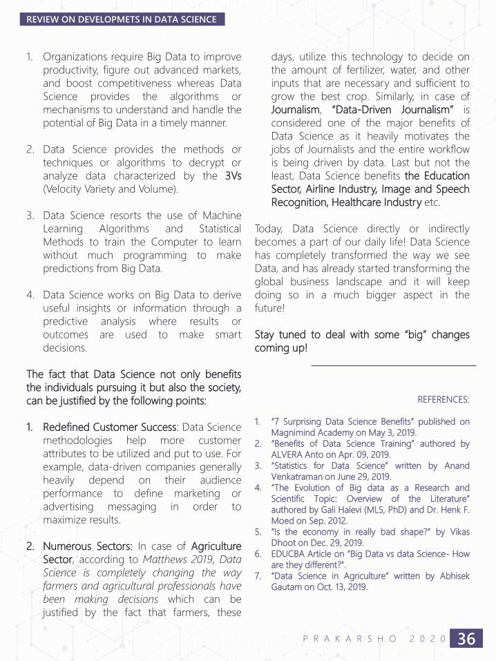
Every Matrix Corresponds to a Graph
To be spoken briefly, Matrix can be represented as a weighted bipartite graph.
Bipartite refers to the dots which come in two different types, (Here for the rows
and columns) and ‘weighted’ refers to each edge which is marked with certain
numbers.
Above is a 3×2matrix (say M) which is well depicted in graphs. For that three dots
for 3 rows and two dots for 2 columns of M are drawn. And edges are drawn
correspondingly for non-zero entries.
A Review On
Matrix and Probability
In Light of Graphs
37P R A K A R S H O 2 0 2 0
Let me try to elaborate the general set up. let,
a matrix M be any array of n×m ordered
members. The array can also be visualized in
terms of a function
M: X × Y → R,
where,
X = {x1, x2, … . . , xn} is a set of n elements
and
Y = {y1, y2, … , ym} is a set of m elements.
Now if I intend to elaborate the matrix M to
you, I need to mention each ijthentry.Necessarily there exists a real Mij for each pair
of indices (i, j). In brief what role a function
itself plays,
M: X × Y → R associates for every pair
(xi, yj).Let us simply write Mij for M(xi, yj).
A Matrix as a Function
Let a matrix M be a function. Then,
M: XxY → R
X={x1, x2, x3}
Y={y1, y2}
I mention we don’t give lines for zero entries
since it has no weightage.
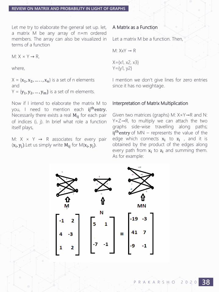
Interpretation of Matrix Multiplication
Given two matrices (graphs) M: X×Y→R and N:
Y×Z→R, to multiply we can attach the two
graphs side-wise travelling along paths;
ijthentry of MN – represents the value of the
edge which connects xi to zi , and it is
obtained by the product of the edges along
every path from xi to zi and summing them.
As for example:
38P R A K A R S H O 2 0 2 0
REVIEW ON MATRIX AND PROBABILITY IN LIGHT OF GRAPHS
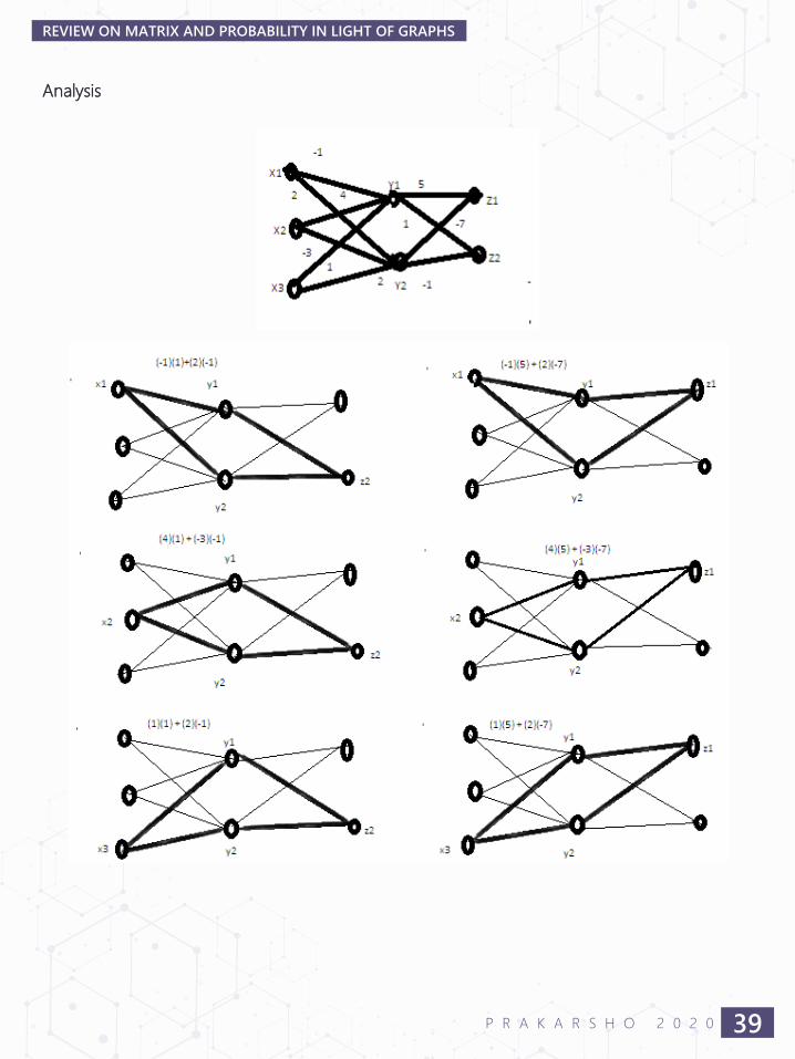
Analysis
39P R A K A R S H O 2 0 2 0
REVIEW ON MATRIX AND PROBABILITY IN LIGHT OF GRAPHS
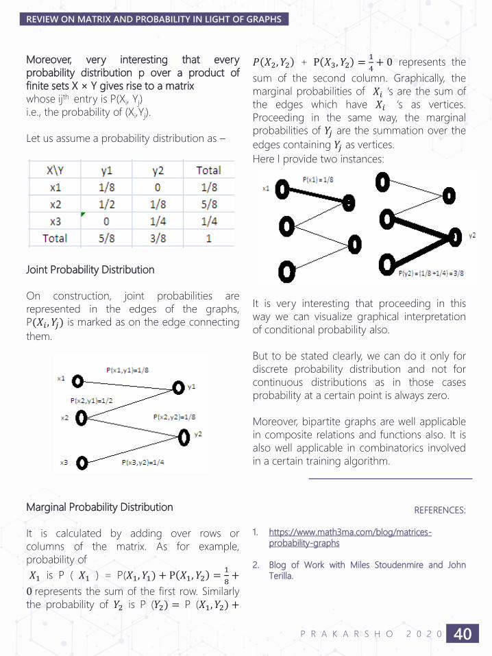
Moreover, very interesting that every
probability distribution p over a product of
finite sets X × Y gives rise to a matrix
whose ijth entry is P(Xi, Yj)
i.e., the probability of (Xi,Yj).
Let us assume a probability distribution as –
Joint Probability Distribution
On construction, joint probabilities are
represented in the edges of the graphs,
P(𝑋𝑖 , 𝑌𝑗) is marked as on the edge connecting
them.
Marginal Probability Distribution
It is calculated by adding over rows or
columns of the matrix. As for example,
probability of
𝑋1 is P ( 𝑋1 ) = P(𝑋1, 𝑌1) + P 𝑋1, 𝑌2 =1
8+
0 represents the sum of the first row. Similarly
the probability of 𝑌2 is P (𝑌2) = P (𝑋1, 𝑌2) +
𝑃 𝑋2, 𝑌2 + P 𝑋3, 𝑌2 =1
4+ 0 represents the
sum of the second column. Graphically, the
marginal probabilities of 𝑋𝑖 ‘s are the sum of
the edges which have 𝑋𝑖 ‘s as vertices.
Proceeding in the same way, the marginal
probabilities of 𝑌𝑗 are the summation over the
edges containing 𝑌𝑗 as vertices.
Here I provide two instances:
It is very interesting that proceeding in this
way we can visualize graphical interpretation
of conditional probability also.
But to be stated clearly, we can do it only for
discrete probability distribution and not for
continuous distributions as in those cases
probability at a certain point is always zero.
Moreover, bipartite graphs are well applicable
in composite relations and functions also. It is
also well applicable in combinatorics involved
in a certain training algorithm.
REFERENCES:
1. https://www.math3ma.com/blog/matrices-
probability-graphs
2. Blog of Work with Miles Stoudenmire and John
Terilla.
40P R A K A R S H O 2 0 2 0
REVIEW ON MATRIX AND PROBABILITY IN LIGHT OF GRAPHS
Utsyo Chakraborty1st year, Department of Statistics
The thought of amalgamating science and music has been a point of debate for
several years. The composer Pierre Boulez (1925-2016) said of this: “It is treason to
mix the two, as science progresses but music does not”. Several philosophers and
critics believe that music is a spontaneous form of art which provides
entertainment and that giving it scientific treatment would suck the life out of it.
There are several detractors to this statement as well. The twentieth century has
time and again proved that it is possible to produce sophisticated music with a
technical approach.
It has been found that there exist several pieces of music which adhere to
principles in physics and mathematics without the composer realizing their
integration into their music. This is generally common in the music of the “Period
of Common Practice” (early 1600s-1900 and slightly after). Two immediate
exceptions from this period come to mind:
1. Erik Satie (1866-1925) used the Golden Ratio (two quantities are in the golden
ratio if their ratio is the same as the ratio of their sum to the larger of the two
quantities, numerically equal to 1.66) to proportion sections of music in his
“Sonneries de la Rose + Croix”.
2. Bela Bartok (1881-1945) used the Fibonacci sequence (if the 1st term of the
sequence is 0 and the 2nd term of the sequence is 1, then the general term of
the sequence is given by 𝑡𝑛 = 𝑡𝑛−1 + 𝑡𝑛−2 with 𝑛 ∈ 𝑁) to fashion rhythms in
his “Music for Strings, Percussion and Celesta”.
That however, has not been the case post the Second World War. There exist
works in which the composer constructs a piece using a particular mathematical
model. Pieces belonging to this category have gained much notoriety due to their
non compliance with tradition. It can produce anomalous “anti-musical” and
Statistics:A Musical Viewpoint
41P R A K A R S H O 2 0 2 0
dadaist effects which has earned it the derision
and wrath of many a listener. However it is
always interesting to analyze and perceive
music from a new viewpoint. This gives it
freshness and a certain vigor which makes the
act of listening exciting. Thus, the main
intention of this article is to throw light on the
development of statistical methods which are
being used in the interpretation of music.
Analysis of Musical Parameters
The most preliminary way of interpreting
music is by means of graphical presentation.
Musical data is nothing but Time Series Data.
Pitches, dynamics and timbre are some of the
parameters which vary as time passes by. A
line diagram can be used for presentation
purposes, with time being represented
horizontally from left to right and pitches
being represented vertically. Due to a large
dispersion in frequencies, the vertical axis can
be taken in a logarithmic fashion. This will
hence indicate relative changes in pitch
instead of absolute ones (such a
representation is called ratio / semi-
logarithmic chart). The horizontal axis can
assume a certain rhythmic or temporal value.
This can greatly help in deducing melodic and
contrapuntal (motion of several independent
musical lines) structures. This also takes into
account rhythmic pulse, another important
parameter in music.
Harmonic content (vertical alignment of music
which gives rise to chords, progressions, etc.)
can be studied by assigning numerical facts
and figures to individual pitches. This is one of
the most elementary concepts of musical set
theory. Such data can be subjected to
statistical analysis, thus bringing out hidden
analogies in music. Here are some recent
studies which elicit my claim.
1. Nakamura and Kaneko by means of a
stochastic model could explain the
evolution in musical style as one
progressed from one time period to
another.
2. Miles, Rosen and Grzywacz could analyze
Harmonic surprise and preferences of
popular music by using Corpus analysis.
3. Krumhansl using univariate, sequential
statistics could geometrically represent
tonalities as the surface of a toroid,
highlighting intervallic relationships like the
cycle of fifths, relative minor/major and
tonic triads.
4. Temperly and Clerq used theoretical
distributions to explain and introduce
harmonic concepts in rock music, like local
harmonic field.
5. David Schiff analyzed the music (using
elementary descriptive procedures) of
Elliott Carter (1908-2012) to show that his
“Night Fantasies” contains an all-interval
twelve tone row (an array of pitches which
can be used in musical construction; such
composition is called serial composition
and was very popular in the twentieth
century)
.
Composition
Besides analysis, composition using statistical
ideas has also been a common point of
interest. The work of Iannis Xenakis (1922-2001)
has been groundbreaking in such regard. His
work “Pithoprakta” (composed in 1955) is his
most elaborate composition using statistical
techniques. Pithoprakta , written for strings,
trombones, xylophone and wood
block, translates to "actions through
probability" The main impetus behind
42P R A K A R S H O 2 0 2 0
STATISTICS: A MUSICAL VIEWPOINT
composition was Bernoulli’s Law of Large
numbers (According to the law, the average of
the results obtained from a large number of
trials should be close to the expected value,
and will tend to become closer to the
expected value as more trials are performed)
and the statistical mechanics of gases. In order
to give this thought a musical existence, he
used the Maxwell-Boltzmann distribution to
assign each instrument as a gas molecule
which freely glides through space in time. He
randomly sampled certain values from the
theoretical distribution by imagining certain
limitations in temperature and pressure and
then plotted them in a two-dimensional graph
with the y-axis showing pitch (0.25 cm= 1
semitone) and the x-axis showing time (5 cm=
1 measure with the tempo quarter note equals
26). Due to this stochastic approach to
composition, each part goes nowhere but the
whole mass of the music follows Bernoulli’s
law.
The above stated technique is in general
cumbersome. However, computer generated
algorithms are now using Markovian Chains
and pattern recognition to form melodies.
These chains can not only produce randomly
generated melodies, but at the same time can
statistically analyze pitches and rhythm to
produce music reminiscent of a particular
composer. An example of this was the Google
Doodle released on the birthday of Johann
Sebastian Bach (1685-1750) which used similar
processes (along with patches of AI and ML)
to provide perfect four-part harmony in the
style of Bach to any randomly inputted
melody. Recent studies use data science in
order to analyze the String Quartets of
Beethoven (1770-1827). The use of fractals in
the music of Gyorgy Ligeti (1926-2006) has
also contributed to a statistical development in
music.
Conclusion
Despite its currently small scale, more and
more studies are being conducted which aim
at developing statistical models in composition
and analysis. This has led to an increased
awareness in the various procedures in music
and thus bringing forward music to a larger
audience. The periodic progress of such
approaches is inculcating new ways of
perceiving music. Music can organically evolve
as a result of such efforts, thus rendering it
revolutionary and making every listener and
composer susceptible to innovative, original
influences and objectives.
SUGGESTED LISTNING:
1. Satie: Sonneries de la Rose + Croix.2. Bartok: Music for Strings, Percussion and Celesta;
Sonata for two pianos and percussion.3. Carter: Night Fantasies4. Ligeti: Clocks and Clouds5. Xenakis: Pithoprakta; Metastaseis
REFERENCES:
1. Symphony with Statistics: Buddha Kinkar Bhaumik2. Statistical Evolutionary Laws in Musical Styles: Eita
Nakamura and Kunihiko Kaneko3. A Statistical Analysis of the Relationship between
Harmonic Surprise and Preference in Popular Music:Miles, Rosen and Grzywacz
4. Statistics, Structure and Style in Music: Carol LynneKrumhansl
5. Statistical Analysis of Harmony and Melody in RockMusic: Temperly and Clerq
6. The Music of Elliott Carter: David Schiff7. Formalized Music: Thoughts and Mathematics in
Composition: Iannis Xenakis8. Decoding Beethoven's music style using data
science: Ecole Polytechnique Fédérale de Lausanne
43P R A K A R S H O 2 0 2 0
STATISTICS: A MUSICAL VIEWPOINT
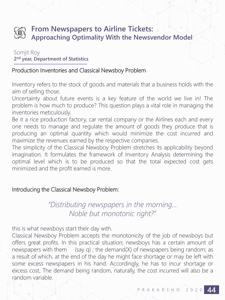
Somjit Roy2nd year, Department of Statistics
Production Inventories and Classical Newsboy Problem
Inventory refers to the stock of goods and materials that a business holds with the
aim of selling those.
Uncertainty about future events is a key feature of the world we live in! The
problem is how much to produce? This question plays a vital role in managing the
inventories meticulously.
Be it a rice production factory, car rental company or the Airlines each and every
one needs to manage and regulate the amount of goods they produce that is
producing an optimal quantity which would minimize the cost incurred and
maximize the revenues earned by the respective companies.
The simplicity of the Classical Newsboy Problem stretches its applicability beyond
imagination. It formulates the framework of Inventory Analysis determining the
optimal level which is to be produced so that the total expected cost gets
minimized and the profit earned is more.
Introducing the Classical Newsboy Problem:
“Distributing newspapers in the morning…
Noble but monotonic right?”
this is what newsboys start their day with.
Classical Newsboy Problem accepts the monotonicity of the job of newsboys but
offers great profits. In this practical situation; newsboys has a certain amount of
newspapers with them (say q) ; the demand(X) of newspapers being random; as
a result of which, at the end of the day he might face shortage or may be left with
some excess newspapers in his hand. Accordingly, he has to incur shortage or
excess cost. The demand being random, naturally, the cost incurred will also be a
random variable.
From Newspapers to Airline Tickets:Approaching Optimality With the Newsvendor Model
44P R A K A R S H O 2 0 2 0
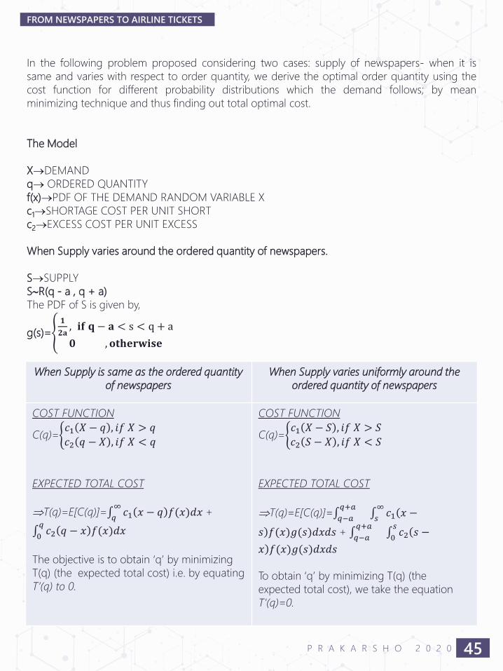
In the following problem proposed considering two cases: supply of newspapers- when it is
same and varies with respect to order quantity, we derive the optimal order quantity using the
cost function for different probability distributions which the demand follows; by mean
minimizing technique and thus finding out total optimal cost.
The Model
X→DEMAND
q→ ORDERED QUANTITY
f(x)→PDF OF THE DEMAND RANDOM VARIABLE X
c1→SHORTAGE COST PER UNIT SHORT
c2→EXCESS COST PER UNIT EXCESS
When Supply varies around the ordered quantity of newspapers.
S→SUPPLY
SR(q - a , q + a)
The PDF of S is given by,
g(s)=ቐ𝟏
𝟐𝐚, 𝐢𝐟 𝐪 − 𝐚 < s < q + a
𝟎 , 𝐨𝐭𝐡𝐞𝐫𝐰𝐢𝐬𝐞
45P R A K A R S H O 2 0 2 0
FROM NEWSPAPERS TO AIRLINE TICKETS
When Supply is same as the ordered quantity
of newspapers
When Supply varies uniformly around the
ordered quantity of newspapers
COST FUNCTION
C(q)=ቊ𝑐1 𝑋 − 𝑞 , 𝑖𝑓 𝑋 > 𝑞
𝑐2 𝑞 − 𝑋 , 𝑖𝑓 𝑋 < 𝑞
EXPECTED TOTAL COST
T(q)=E[C(q)]=𝑞
∞𝑐1 𝑥 − 𝑞 𝑓(𝑥)𝑑𝑥 +
0
𝑞𝑐2 𝑞 − 𝑥 𝑓(𝑥)𝑑𝑥
The objective is to obtain ‘q’ by minimizing
T(q) (the expected total cost) i.e. by equating
T’(q) to 0.
COST FUNCTION
C(q)=ቊ𝑐1 𝑋 − 𝑆 , 𝑖𝑓 𝑋 > 𝑆
𝑐2 𝑆 − 𝑋 , 𝑖𝑓 𝑋 < 𝑆
EXPECTED TOTAL COST
T(q)=E[C(q)]=𝑞−𝑎
𝑞+𝑎𝑠
∞𝑐1(
)
𝑥 −
𝑠 𝑓(𝑥)𝑔(𝑠)𝑑𝑥𝑑𝑠 +𝑞−𝑎
𝑞+𝑎0
𝑠𝑐2(
)
𝑠 −
𝑥 𝑓(𝑥)𝑔(𝑠)𝑑𝑥𝑑𝑠
To obtain ‘q’ by minimizing T(q) (the
expected total cost), we take the equation
T’(q)=0.
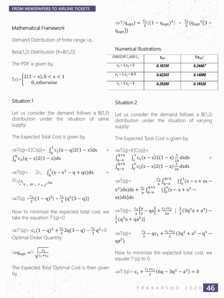
Mathematical Framework
Demand Distribution of finite range i.e.,
Beta(1,2) Distribution [XB(1,2)]
The PDF is given by,
f(x)=ቊ2 1 − x , 0 < x < 1
0, otherwise
Situation 1
Let us consider the demand follows a B(1,2)
distribution under the situation of same
supply:
The Expected Total Cost is given by,
T(q)=E[C(q)]= q
1c1 x − q 2 1 − x dx +
0
qc2 q − x 2 1 − x dx
T(q)= 2c1 q
1(x − x2 − q + qx)dx +
2c20
q
q − qx − x + x2 dx
T(q) =c1
3{(1 − q)3} +
c2
3{q2 3 − q }
Now to minimize the expected total cost, we
take the equation T’(q)=0
T’(q)=-c1(1 − q)2 +c2
32q 3 − q −
c2
3q2=0
Optimal Order Quantity:
qopt =1-c2
c1+c2
The Expected Total Optimal Cost is then given
by,
T(qopt) =c1
3{(1 − qopt)
3 } +c2
3{qopt
2൫
൯
3 −
qopt }
Numerical Illustrations
Situation 2
Let us consider the demand follows a B(1,2)
distribution under the situation of varying
supply:
The Expected Total Cost is given by,
T(q)=E[C(q)]=
q−a
q+as
1c1 x − s 2(1 − x)
1
2adxds +
q−a
q+a0
sc2 s − x 2(1 − x)
1
2adxds
T(q)=c1
aq−a
q+a}s
1(
)
x − s + sx −
x2 dx}ds +c2
aq−a
q+a}0
s(
)
s − x + x2 −
sx dx}ds
T(q)=c1
a
a
3− qa +
c1+c2
2a[
2
33q2a + a3 −
2
3(q3a + qa3)]
T(q)=c1
3− qc1 +
c1+c2
3(
)
3q2 + a2 − q3 −
qa2
Now to minimize the expected total cost, we
equate T’(q) to 0.
T’(q)=-c1 +c1+c2
36q − 3q2 − a2 = 0
46P R A K A R S H O 2 0 2 0
FROM NEWSPAPERS TO AIRLINE TICKETS
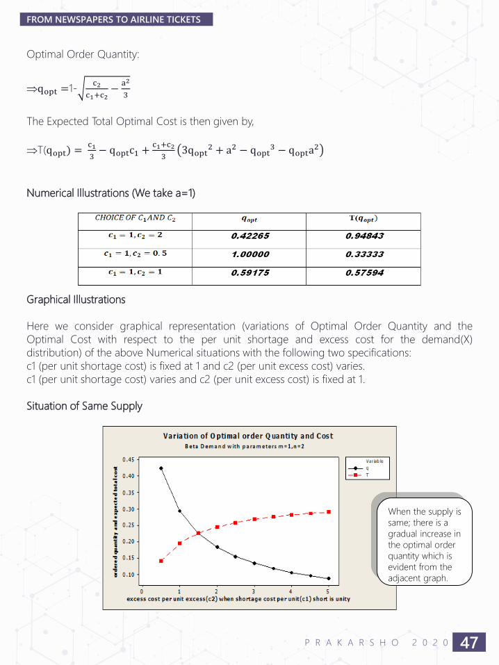
Optimal Order Quantity:
qopt =1-c2
c1+c2−
a2
3
The Expected Total Optimal Cost is then given by,
T(qopt) =c1
3− qoptc1 +
c1+c2
33qopt
2 + a2 − qopt3 − qopta
2
Numerical Illustrations (We take a=1)
Graphical Illustrations
Here we consider graphical representation (variations of Optimal Order Quantity and the
Optimal Cost with respect to the per unit shortage and excess cost for the demand(X)
distribution) of the above Numerical situations with the following two specifications:
c1 (per unit shortage cost) is fixed at 1 and c2 (per unit excess cost) varies.
c1 (per unit shortage cost) varies and c2 (per unit excess cost) is fixed at 1.
Situation of Same Supply
47P R A K A R S H O 2 0 2 0
FROM NEWSPAPERS TO AIRLINE TICKETS
When the supply is
same; there is a
gradual increase in
the optimal order
quantity which is
evident from the
adjacent graph.
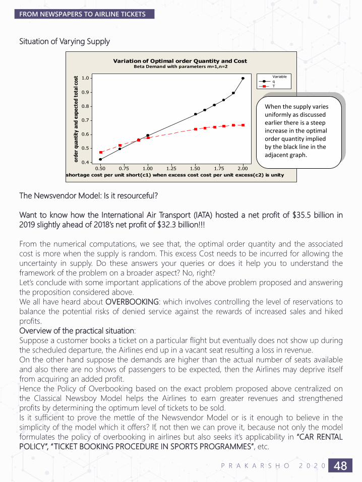
Situation of Varying Supply
The Newsvendor Model: Is it resourceful?
Want to know how the International Air Transport (IATA) hosted a net profit of $35.5 billion in
2019 slightly ahead of 2018’s net profit of $32.3 billion!!!
From the numerical computations, we see that, the optimal order quantity and the associated
cost is more when the supply is random. This excess Cost needs to be incurred for allowing the
uncertainty in supply. Do these answers your queries or does it help you to understand the
framework of the problem on a broader aspect? No, right?
Let’s conclude with some important applications of the above problem proposed and answering
the proposition considered above.
We all have heard about OVERBOOKING: which involves controlling the level of reservations to
balance the potential risks of denied service against the rewards of increased sales and hiked
profits.
Overview of the practical situation:
Suppose a customer books a ticket on a particular flight but eventually does not show up during
the scheduled departure, the Airlines end up in a vacant seat resulting a loss in revenue.
On the other hand suppose the demands are higher than the actual number of seats available
and also there are no shows of passengers to be expected, then the Airlines may deprive itself
from acquiring an added profit.
Hence the Policy of Overbooking based on the exact problem proposed above centralized on
the Classical Newsboy Model helps the Airlines to earn greater revenues and strengthened
profits by determining the optimum level of tickets to be sold.
Is it sufficient to prove the mettle of the Newsvendor Model or is it enough to believe in the
simplicity of the model which it offers? If, not then we can prove it, because not only the model
formulates the policy of overbooking in airlines but also seeks it’s applicability in “CAR RENTAL
POLICY”, “TICKET BOOKING PROCEDURE IN SPORTS PROGRAMMES”, etc.
48P R A K A R S H O 2 0 2 0
FROM NEWSPAPERS TO AIRLINE TICKETS
2.001.751.501.251.000.750.50
1.0
0.9
0.8
0.7
0.6
0.5
0.4
shortage cost per unit short(c1) when excess cost cost per unit excess(c2) is unity
ord
er
qu
an
tity
an
d e
xpe
cte
d t
ota
l co
stq
T
Variable
Variation of Optimal order Quantity and Cost Beta Demand with parameters m=1,n=2
When the supply varies uniformly as discussed earlier there is a steep increase in the optimal order quantity implied by the black line in the adjacent graph.

Dhruvi Mundra2nd year, Department of Statistics
“There is only one boss. The customer.
And he can fire everybody in the company
from the chairman on down, simply by spending his
money somewhere else.”-Sam Walton
Companies spend most of their time and effort in acquiring new customers.
However, the cost of retaining a customer is 5 times cheaper than acquiring a new
one. Customer retention is the method of analysing how many companies
continue to buy from you and are therefore
loyal to your brand. Churn is on the other end
of the spectrum. It’s the method of finding out
how many customers stop buying from your
company.
With the coming up of multiple new video
streaming platforms like Amazon Prime
Video, Hulu, HBO, Hotstar, etc, it is becoming
very difficult for Subscription Video On
Demand (SVOD) companies to retain its
customer base. Netflix is the only SVOD
company having positive retention. Rivals
like Amazon Prime Video, Hulu, AT&T owned
by HBO now are facing a higher churn rate
than Netflix. While they are spending a lot
How Does Netflix Use Analytics
To Prevent Churn
49P R A K A R S H O 2 0 2 0
of their resources on acquiring new customers,
they don’t do anything to stop the Churn rate
once the free trial is over. Let us see how,
amidst rising competition, is Netflix preventing
Churn.
Netflix uses a strategy called Customer
Journey Analytics.
A third of the US households have an active
Netflix subscription. Recent research by Parks
Associates showed that only 4% of U.S.
broadband households cancelled their Netflix
service — representing almost 9% of Netflix’s
subscriber base. Netflix achieved this by using
a strategy called Customer Journey Analytics.
What is Customer Journey Analytics?
Customer journey analytics is the process that
companies use to understand users at an
individual and personal level in order to give
them the best user experience. They do this by
analysing the user’s interaction with the
company through various channels. Using the
data collected, they try to understand the
preferences of the user.
How is Netflix using this process to retain
customers?
Netflix asks its users if it wants to continue with
the subscription at the end of every month. It
is very easy to lose customers this way. This
option given to the users makes it even more
crucial for Netflix to ensure that its users
remain loyal to them. They ensure that the
users don’t only use Netflix for a trial period
but subscribe and actively continue using it.
Netflix ensures to provide the users with a
wide variety of shows and movies to keep
them hooked. But apart from this, Netflix also
studies the users very carefully. These are few
of the things they collect data on:
• Which shows you watch
• If you finish the entire season or not
• Where you pause, fast forward, rewind, etc
• If you leave an episode midway, how long
does it take for you to come back and
restart it? If you even restart it.
• How long does it take for you to complete
an entire season
• Which day of the week do you watch the
shows
• There are speculations that it also collects
data on brightness, volume level, movie
settings, etc
Using these, they try to create a personalized
experience for you. They recommend you
shows based on your watch history. The
trailers of these new shows are also
personalized just for you. For example, when
House of Cards was released on Netflix,
different viewers were exposed to different
trailers. If your search history showed that you
were a David Fincher fan (the director of
House of Cards), trailers portraying his best-
directing skills were shown to you. If you had
viewed films with Kevin Spacey, then your
trailer centered around him.
Well, this is for the users who are already
actively watching Netflix.
What about those who have stopped
watching Netflix?
Email notifications:
Users are notified about new shows being
added, depending on your watch history,
50P R A K A R S H O 2 0 2 0
NETFLIX CHURN PREVENTION

through your emails. These emails are specially
designed. They don’t just inform you about
the show, but also give you an option to
“watch it now” or “add it to your playlist”. This
helps in direct and fast conversion of users
who weren’t active on Netflix, to open the
app/site and watch the series.
Push notifications:
No one usually likes push notifications. To get
the attention of the user, the push notifications
are designed in a very simple and
straightforward way. It informs you of a new
season of a show being added (depending
upon your watch history).
Every user is reluctant to changes made on
the app. Humans, in general, resist changes.
Every new feature added is first tested using
split testing where Netflix randomly selects
300,000 users from around the world and
introduces this feature to them. The reactions
are then studied. Netflix also gives every user
a demo every time a new feature gets added
so that they become comfortable with the
changes.
Whenever a show is recommended to you,
Netflix has only 90 seconds to convince you to
start watching it. Their trailer needs to be as
personalized for you as possible.
Even still, with so many options to keep users
informed across nearly every type of device,
Netflix is continuing to test, innovate and
refine its algorithms to prevent churn and
keep users watching — and those users are at
its core in a quest for never-ending user
experience growth.
REFERENCES:
1. https://neilpatel.com/blog/how-netflix-maintains-
low-churn/
2. https://www.pointillist.com/blog/reduce-churn-
customer-journey-analytics/
3. https://www.muvi.com/blogs/ott-churn-
management-strategy-like-netflix.html
51P R A K A R S H O 2 0 2 0
NETFLIX CHURN PREVENTION
Esha Mandal, Soham Ganguly1st year, Department of Statistics
If you are in the statistics department and you are highly satisfied after choosing
statistics you are more likely to prefer back gate over front gate. Sounds very
“nonsensical” isn't it ? This is the world of spurious correlation. Our objectives to
have a peep into this funny World.
In real life we often find variables which are expected to be uncorrelated but on
measuring they are found to be correlated which makes no sense. These types of
correlation are called Spurious Correlation or nonsense correlation which leads to
serious interpretation fallacy. One thing that should be noted is that correlation
doesn't imply causation. If two variables are correlated doesn't imply that one has
caused the other variable to change.
There may be a pair of data which are affected in the same or opposite manner
by a third hidden variable called the “Lurking Variable”.
Spurious Correlation: A Few Interesting Examples
Spurious correlations are often very obvious and are thus often unnoticed by most
people for example number of cars on road v/s infant mortality rate. Here time is
the lurking variable which is the most common known lurking variable since time
progresses number of cars increases and infant mortality decreases Nonsense
correlation can be observed between bivariate data as well as other kinds of data.
For eg:
❏ If we consider a group of children between the age 5-15, then we will find an
unexpected correlation between the two variables
X: Shoe Size Y: Marks in a handwriting competition,
Lurking Variable : Age
Expecting the Unexpected
52P R A K A R S H O 2 0 2 0
❏ X: Time needed to cook
Y: Tendency to have breathing problems
Lurking Variable: Altitude of place
Spurious Correlation In Our STSA Department
We thought to find out some of the hidden
correlations that could be found in our
department, so for it a questionnaire was
formed. Data collection:
Google forms were forwarded to all students
of STSA Departments
● Name, Roll Number, Semester
● Total credit hours collected
● On a scale of 1 to 5 how much are you
satisfied after choosing Statistics
● On a scale of 1 to 5 how much do you prefer
using back gate over front gate
● Hours devoted per day for competitive
exam preparation
● % of hours (Out of total study hours)
devoted to study General Elective(GE)
Forms were forwarded via social media The
response rate was moderate.
The data was copied to minitab and the
following scatterplots were drawn and
observed
(i) Credit hours v/s time devoted for
competitive exam preparations In this
case, we found that students with more
credit points, invested more time for
competitive exam preparation.
(ii) Credit hours v/s time devoted to learn GE.
In this case, we found that as credit hours
increased, students tended to invest more
time for studying GE subjects.
(iii) Satisfied after choosing statistics and
preference of back gate. As stated in the
beginning, those who are highly satisfied
after choosing statistics, are more likely to
prefer back gate over front gate.
All the above correlations may logically seem
unreal but few of them are rather very
obvious. As mentioned earlier, correlation
doesn’t imply causation. So we should not
draw absurd conclusions such as one has
caused the other variable to change. These
correlations are just a consequence of the
impact of a third lurking variable.
Correlation (i) and (ii) is the outcome of the
third variable: The year in which the student
studies.
As the year of a student progresses:
1) Number of credit hours collected increases
2) Time devoted for competitive exam
preparation increases.
3) Time devoted to study GE decreases( since
1st year students tend to devote more time
in studying maths than 2nd year students
do in studying comp/eco. Also 3rd year
students don’t have GE at all.)
One thing is to be revealed. We had
mentioned in the google forms that 5 people
among the ones whose both the answers will
be the same will be given a gift. This
influenced not all but many of the respondents
to answer in that manner. Thus on obtaining
the scatterplot the data points tended to
cluster around the line y=x. This gave birth to
the absurd positive linear relationship given in
(iii) with the lurking variable being none other
than Us: The framers of the question. Here we
made a few assumptions that the variables
were not originally correlated and it is entirely
our manipulation that caused the correlation.
So in this article, we intended to illustrate how
widespread nonsense correlation is but is
often left unnoticed in practice. We tried to
53P R A K A R S H O 2 0 2 0
EXPECTING THE UNEXPECTED

demonstrate how there may be much more
complicated cases than just cause-effect
relationships. Correlations may be caused by a
third hidden FACTOR and thus illogical
correlations should not mislead us to draw
false conclusions. We would like to end this
article by quoting a paragraph from Darrell
Huff’s well known classic ‘How to lie with
Statistics’
"Permitting statistical treatment and the
hypnotic presence of numbers and decimal
points to befog causal relationships is little
better than superstition. And it is often more
seriously misleading. It is rather like the
conviction among the people of the New
Hebrides that body lice produce good health.
Observation over the centuries had taught
them that people in good health usually had
lice and sick people very often did not. The
observation itself was accurate and sound, as
observations made informally over the years
surprisingly often are. Not so much can be
said for the conclusion to which these
primitive people came from their evidence:
Lice make a man healthy. Everybody should
have them. As we have already noted,
scantier evidence than this— treated in the
statistical mill until common sense could no
longer penetrate to it—has made many a
medical fortune and many a medical article in
magazines, including professional ones. More
sophisticated observers finally got things
straightened out in the New Hebrides. As it
turned out, almost everybody in those circles
had lice most of the time. It was, you might
say, the normal condition of man. When,
however' anyone took a fever (quite possibly
carried to him by those same lice) and his
body became too hot for comfortable
habitation, the lice left. There you have cause
and effect altogether confusingly distorted,
reversed, and intermingled.“
REFERENCE:
How to lie with Statistics, Darrell Huff
54P R A K A R S H O 2 0 2 0
EXPECTING THE UNEXPECTED
Shrayan Roy1st year, Department of Statistics
The world is based on visualization. Visualizing something, we understand the
facts behind or gain some knowledge from it. If we face some problems due to
some issues, we try to find the solution for that and when the problem is solved if
the situation comes again in future, we solve the problems using past experience.
Similarly, while handling a dataset, we need to know the characteristics of the data,
How the data behaves, what are the features?
• Is it large?
• What is the tendency?
• How scattered the data is?
• Is there any unusual points or outliers?
• What is the relationship or association between variables? etc.
And the need varies from one dataset to another. Although there are some
statistical measures for that but data visualization is the better method to
comprehend what data reveals to us. We cannot apply any statistical method for
analyzing a dataset, before we know it well. For example, we cannot use moment
measures i.e., mean as a measure of central tendency or standard deviation as a
measure of dispersion without knowing that, whether the data is extremely skewed
or it contains outliers. It is due to non-robustness and non-resistance of mean and
standard deviation.
Thus, it is primary tusk to visualize data after collecting it. According to John W.
Tukey “Three of the main strategies of data analysis are:
1. graphical presentation.
2. provision of flexibility in viewpoint and in facilities,
3. intensive search for parsimony and simplicity.” and he introduced this part of
descriptive statistics as Exploratory Data Analysis (EDA).
Uses of Graphs In EDA
55P R A K A R S H O 2 0 2 0
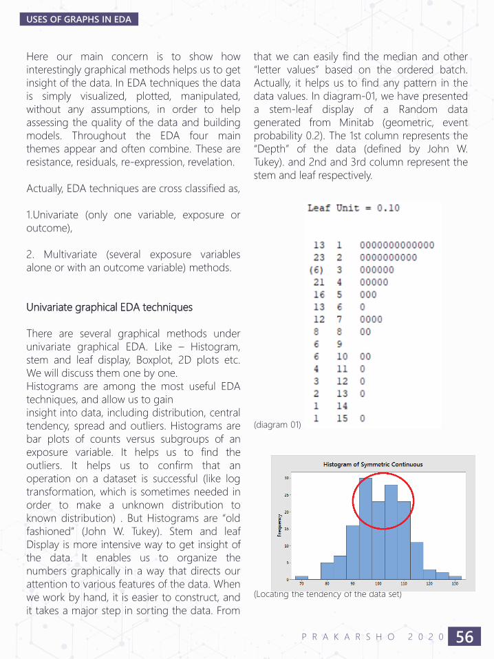
Here our main concern is to show how
interestingly graphical methods helps us to get
insight of the data. In EDA techniques the data
is simply visualized, plotted, manipulated,
without any assumptions, in order to help
assessing the quality of the data and building
models. Throughout the EDA four main
themes appear and often combine. These are
resistance, residuals, re-expression, revelation.
Actually, EDA techniques are cross classified as,
1.Univariate (only one variable, exposure or
outcome),
2. Multivariate (several exposure variables
alone or with an outcome variable) methods.
Univariate graphical EDA techniques
There are several graphical methods under
univariate graphical EDA. Like – Histogram,
stem and leaf display, Boxplot, 2D plots etc.
We will discuss them one by one.
Histograms are among the most useful EDA
techniques, and allow us to gain
insight into data, including distribution, central
tendency, spread and outliers. Histograms are
bar plots of counts versus subgroups of an
exposure variable. It helps us to find the
outliers. It helps us to confirm that an
operation on a dataset is successful (like log
transformation, which is sometimes needed in
order to make a unknown distribution to
known distribution) . But Histograms are “old
fashioned” (John W. Tukey). Stem and leaf
Display is more intensive way to get insight of
the data. It enables us to organize the
numbers graphically in a way that directs our
attention to various features of the data. When
we work by hand, it is easier to construct, and
it takes a major step in sorting the data. From
that we can easily find the median and other
“letter values” based on the ordered batch.
Actually, it helps us to find any pattern in the
data values. In diagram-01, we have presented
a stem-leaf display of a Random data
generated from Minitab (geometric, event
probability 0.2). The 1st column represents the
“Depth” of the data (defined by John W.
Tukey). and 2nd and 3rd column represent the
stem and leaf respectively.
(diagram 01)
(Locating the tendency of the data set)
56P R A K A R S H O 2 0 2 0
USES OF GRAPHS IN EDA
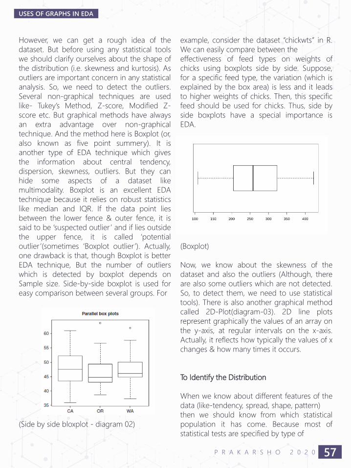
However, we can get a rough idea of the
dataset. But before using any statistical tools
we should clarify ourselves about the shape of
the distribution (i.e. skewness and kurtosis). As
outliers are important concern in any statistical
analysis. So, we need to detect the outliers.
Several non-graphical techniques are used
like- Tukey’s Method, Z-score, Modified Z-
score etc. But graphical methods have always
an extra advantage over non-graphical
technique. And the method here is Boxplot (or,
also known as five point summery). It is
another type of EDA technique which gives
the information about central tendency,
dispersion, skewness, outliers. But they can
hide some aspects of a dataset like
multimodality. Boxplot is an excellent EDA
technique because it relies on robust statistics
like median and IQR. If the data point lies
between the lower fence & outer fence, it is
said to be ‘suspected outlier ’ and if lies outside
the upper fence, it is called ‘potential
outlier ’(sometimes ‘Boxplot outlier ’). Actually,
one drawback is that, though Boxplot is better
EDA technique, But the number of outliers
which is detected by boxplot depends on
Sample size. Side-by-side boxplot is used for
easy comparison between several groups. For
(Side by side bloxplot - diagram 02)
example, consider the dataset “chickwts” in R.
We can easily compare between the
effectiveness of feed types on weights of
chicks using boxplots side by side. Suppose,
for a specific feed type, the variation (which is
explained by the box area) is less and it leads
to higher weights of chicks. Then, this specific
feed should be used for chicks. Thus, side by
side boxplots have a special importance is
EDA.
(Boxplot)
Now, we know about the skewness of the
dataset and also the outliers (Although, there
are also some outliers which are not detected.
So, to detect them, we need to use statistical
tools). There is also another graphical method
called 2D-Plot(diagram-03). 2D line plots
represent graphically the values of an array on
the y-axis, at regular intervals on the x-axis.
Actually, it reflects how typically the values of x
changes & how many times it occurs.
To Identify the Distribution
When we know about different features of the
data (like-tendency, spread, shape, pattern)
then we should know from which statistical
population it has come. Because most of
statistical tests are specified by type of
57P R A K A R S H O 2 0 2 0
USES OF GRAPHS IN EDA
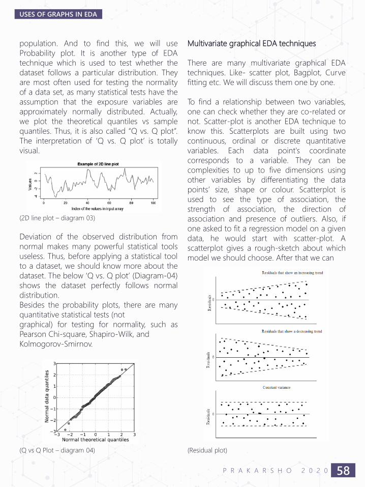
population. And to find this, we will use
Probability plot. It is another type of EDA
technique which is used to test whether the
dataset follows a particular distribution. They
are most often used for testing the normality
of a data set, as many statistical tests have the
assumption that the exposure variables are
approximately normally distributed. Actually,
we plot the theoretical quantiles vs sample
quantiles. Thus, it is also called “Q vs. Q plot”.
The interpretation of ‘Q vs. Q plot’ is totally
visual.
(2D line plot – diagram 03)
Deviation of the observed distribution from
normal makes many powerful statistical tools
useless. Thus, before applying a statistical tool
to a dataset, we should know more about the
dataset. The below ‘Q vs. Q plot’ (Diagram-04)
shows the dataset perfectly follows normal
distribution.
Besides the probability plots, there are many
quantitative statistical tests (not
graphical) for testing for normality, such as
Pearson Chi-square, Shapiro-Wilk, and
Kolmogorov-Smirnov.
(Q vs Q Plot – diagram 04)
Multivariate graphical EDA techniques
There are many multivariate graphical EDA
techniques. Like- scatter plot, Bagplot, Curve
fitting etc. We will discuss them one by one.
To find a relationship between two variables,
one can check whether they are co-related or
not. Scatter-plot is another EDA technique to
know this. Scatterplots are built using two
continuous, ordinal or discrete quantitative
variables. Each data point's coordinate
corresponds to a variable. They can be
complexities to up to five dimensions using
other variables by differentiating the data
points’ size, shape or colour. Scatterplot is
used to see the type of association, the
strength of association, the direction of
association and presence of outliers. Also, if
one asked to fit a regression model on a given
data, he would start with scatter-plot. A
scatterplot gives a rough-sketch about which
model we should choose. After that we can
(Residual plot)
58P R A K A R S H O 2 0 2 0
USES OF GRAPHS IN EDA
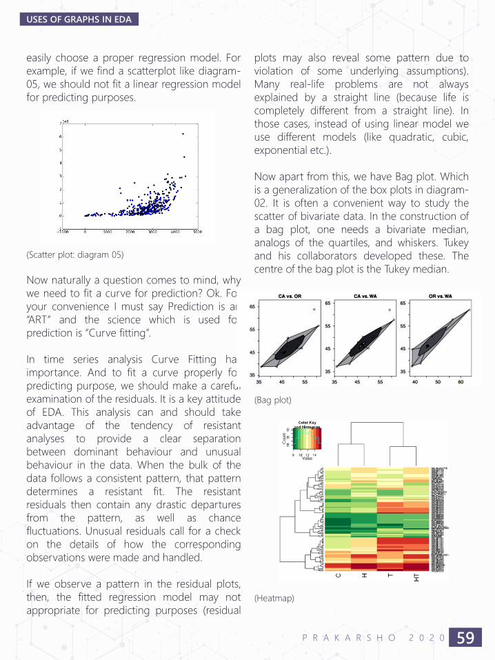
easily choose a proper regression model. For
example, if we find a scatterplot like diagram-
05, we should not fit a linear regression model
for predicting purposes.
(Scatter plot: diagram 05)
Now naturally a question comes to mind, why
we need to fit a curve for prediction? Ok. For
your convenience I must say Prediction is an
“ART” and the science which is used for
prediction is “Curve fitting”.
In time series analysis Curve Fitting has
importance. And to fit a curve properly for
predicting purpose, we should make a careful
examination of the residuals. It is a key attitude
of EDA. This analysis can and should take
advantage of the tendency of resistant
analyses to provide a clear separation
between dominant behaviour and unusual
behaviour in the data. When the bulk of the
data follows a consistent pattern, that pattern
determines a resistant fit. The resistant
residuals then contain any drastic departures
from the pattern, as well as chance
fluctuations. Unusual residuals call for a check
on the details of how the corresponding
observations were made and handled.
If we observe a pattern in the residual plots,
then, the fitted regression model may not
appropriate for predicting purposes (residual
plots may also reveal some pattern due to
violation of some underlying assumptions).
Many real-life problems are not always
explained by a straight line (because life is
completely different from a straight line). In
those cases, instead of using linear model we
use different models (like quadratic, cubic,
exponential etc.).
Now apart from this, we have Bag plot. Which
is a generalization of the box plots in diagram-
02. It is often a convenient way to study the
scatter of bivariate data. In the construction of
a bag plot, one needs a bivariate median,
analogs of the quartiles, and whiskers. Tukey
and his collaborators developed these. The
centre of the bag plot is the Tukey median.
(Bag plot)
(Heatmap)
59P R A K A R S H O 2 0 2 0
USES OF GRAPHS IN EDA
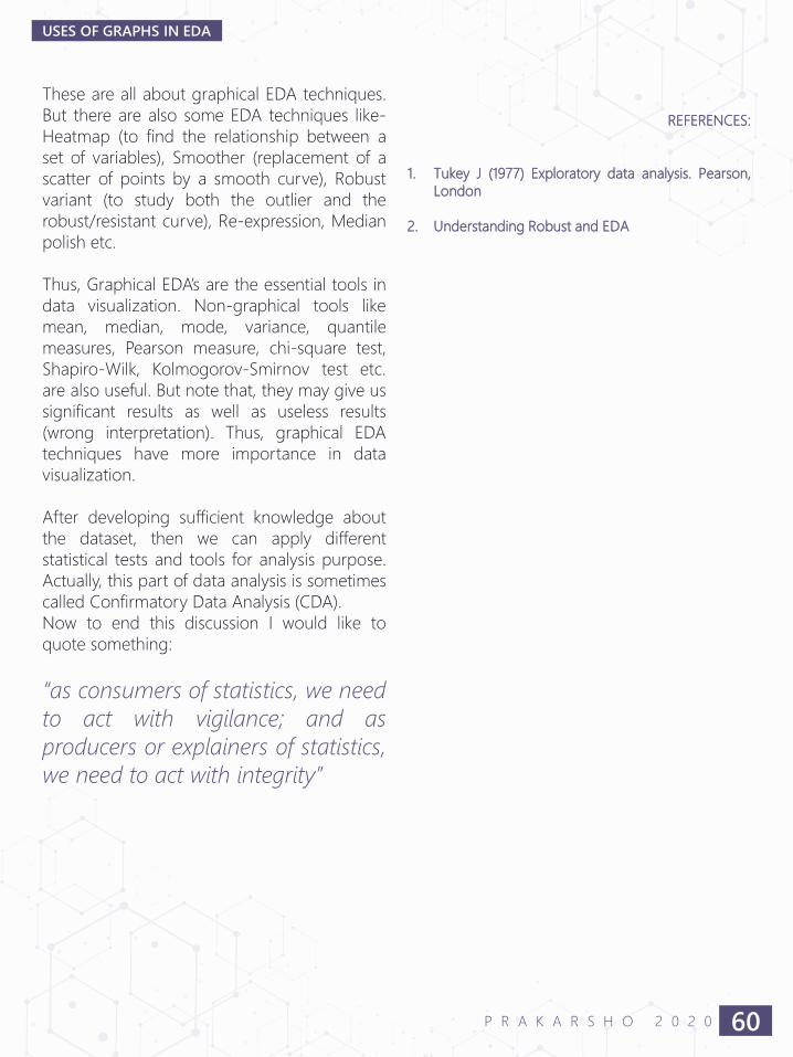
These are all about graphical EDA techniques.
But there are also some EDA techniques like-
Heatmap (to find the relationship between a
set of variables), Smoother (replacement of a
scatter of points by a smooth curve), Robust
variant (to study both the outlier and the
robust/resistant curve), Re-expression, Median
polish etc.
Thus, Graphical EDA’s are the essential tools in
data visualization. Non-graphical tools like
mean, median, mode, variance, quantile
measures, Pearson measure, chi-square test,
Shapiro-Wilk, Kolmogorov-Smirnov test etc.
are also useful. But note that, they may give us
significant results as well as useless results
(wrong interpretation). Thus, graphical EDA
techniques have more importance in data
visualization.
After developing sufficient knowledge about
the dataset, then we can apply different
statistical tests and tools for analysis purpose.
Actually, this part of data analysis is sometimes
called Confirmatory Data Analysis (CDA).
Now to end this discussion I would like to
quote something:
“as consumers of statistics, we need
to act with vigilance; and as
producers or explainers of statistics,
we need to act with integrity”
REFERENCES:
1. Tukey J (1977) Exploratory data analysis. Pearson,
London
2. Understanding Robust and EDA
60P R A K A R S H O 2 0 2 0
USES OF GRAPHS IN EDA
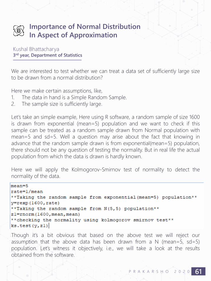
Kushal Bhattacharya3rd year, Department of Statistics
We are interested to test whether we can treat a data set of sufficiently large size
to be drawn from a normal distribution?
Here we make certain assumptions, like,
1. The data in hand is a Simple Random Sample.
2. The sample size is sufficiently large.
Let’s take an simple example, Here using R software, a random sample of size 1600
is drawn from exponential (mean=5) population and we want to check if this
sample can be treated as a random sample drawn from Normal population with
mean=5 and sd=5. Well a question may arise about the fact that knowing in
advance that the random sample drawn is from exponential(mean=5) population,
there should not be any question of testing the normality. But in real life the actual
population from which the data is drawn is hardly known.
Here we will apply the Kolmogorov-Smirnov test of normality to detect the
normality of the data.
Though it’s a bit obvious that based on the above test we will reject our
assumption that the above data has been drawn from a N (mean=5, sd=5)
population. Let’s witness it objectively, i.e., we will take a look at the results
obtained from the software.
Importance of Normal Distribution
In Aspect of Approximation
61P R A K A R S H O 2 0 2 0
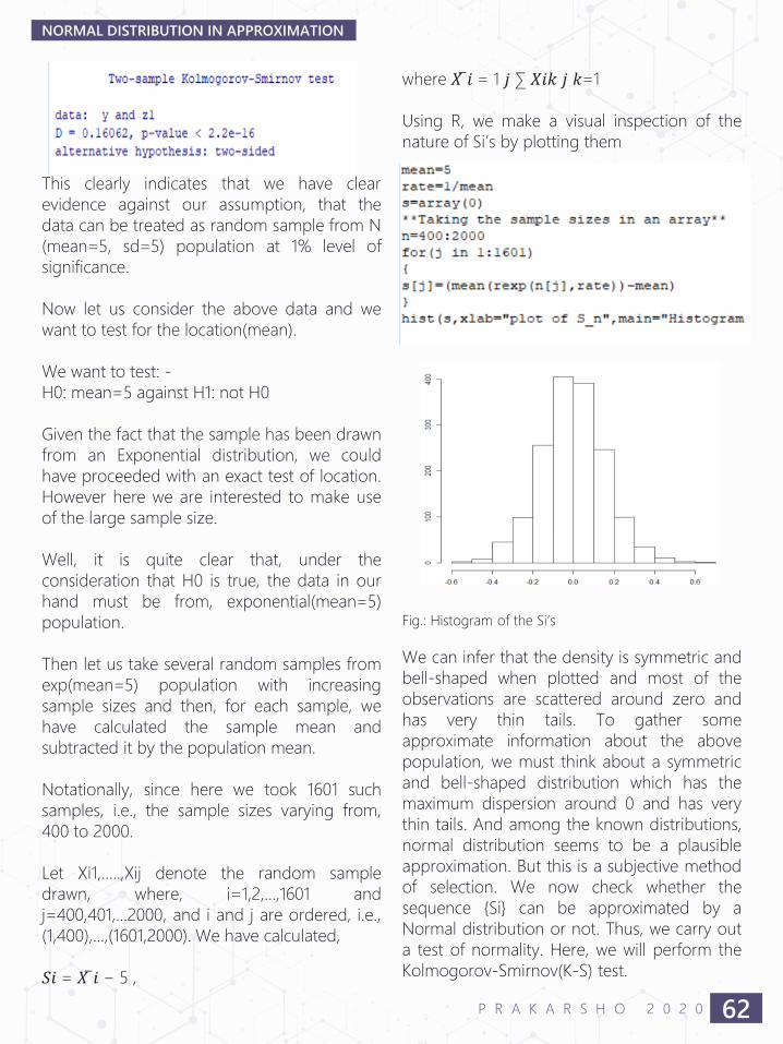
This clearly indicates that we have clear
evidence against our assumption, that the
data can be treated as random sample from N
(mean=5, sd=5) population at 1% level of
significance.
Now let us consider the above data and we
want to test for the location(mean).
We want to test: -
H0: mean=5 against H1: not H0
Given the fact that the sample has been drawn
from an Exponential distribution, we could
have proceeded with an exact test of location.
However here we are interested to make use
of the large sample size.
Well, it is quite clear that, under the
consideration that H0 is true, the data in our
hand must be from, exponential(mean=5)
population.
Then let us take several random samples from
exp(mean=5) population with increasing
sample sizes and then, for each sample, we
have calculated the sample mean and
subtracted it by the population mean.
Notationally, since here we took 1601 such
samples, i.e., the sample sizes varying from,
400 to 2000.
Let Xi1,…..,Xij denote the random sample
drawn, where, i=1,2,…,1601 and
j=400,401,…2000, and i and j are ordered, i.e.,
(1,400),…,(1601,2000). We have calculated,
𝑆𝑖 = 𝑋 ̅ 𝑖 − 5 ,
where 𝑋 ̅ 𝑖 = 1 𝑗 ∑ 𝑋𝑖𝑘 𝑗 𝑘=1
Using R, we make a visual inspection of the
nature of Si’s by plotting them
Fig.: Histogram of the Si’s
We can infer that the density is symmetric and
bell-shaped when plotted and most of the
observations are scattered around zero and
has very thin tails. To gather some
approximate information about the above
population, we must think about a symmetric
and bell-shaped distribution which has the
maximum dispersion around 0 and has very
thin tails. And among the known distributions,
normal distribution seems to be a plausible
approximation. But this is a subjective method
of selection. We now check whether the
sequence {Si} can be approximated by a
Normal distribution or not. Thus, we carry out
a test of normality. Here, we will perform the
Kolmogorov-Smirnov(K-S) test.
62P R A K A R S H O 2 0 2 0
NORMAL DISTRIBUTION IN APPROXIMATION
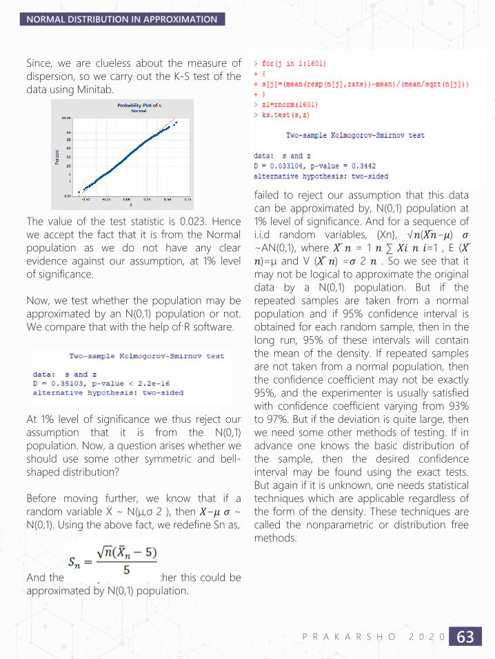
Since, we are clueless about the measure of
dispersion, so we carry out the K-S test of the
data using Minitab.
The value of the test statistic is 0.023. Hence
we accept the fact that it is from the Normal
population as we do not have any clear
evidence against our assumption, at 1% level
of significance.
Now, we test whether the population may be
approximated by an N(0,1) population or not.
We compare that with the help of R software.
At 1% level of significance we thus reject our
assumption that it is from the N(0,1)
population. Now, a question arises whether we
should use some other symmetric and bell-
shaped distribution?
Before moving further, we know that if a
random variable X ~ N(μ,σ 2 ), then 𝑋−𝜇 𝜎 ~
N(0,1). Using the above fact, we redefine Sn as,
And then we try to test whether this could be
approximated by N(0,1) population.
The value of D is 0.033104. Hence, we have
failed to reject our assumption that this data
can be approximated by, N(0,1) population at
1% level of significance. And for a sequence of
i.i.d random variables, {Xn}, √𝑛(𝑋 ̅𝑛−𝜇) 𝜎~AN(0,1), where �̅� 𝑛 = 1 𝑛 ∑ 𝑋𝑖 𝑛 𝑖=1 , E (𝑋 ̅
𝑛)=μ and V (�̅� 𝑛) =𝜎 2 𝑛 . So we see that it
may not be logical to approximate the original
data by a N(0,1) population. But if the
repeated samples are taken from a normal
population and if 95% confidence interval is
obtained for each random sample, then in the
long run, 95% of these intervals will contain
the mean of the density. If repeated samples
are not taken from a normal population, then
the confidence coefficient may not be exactly
95%, and the experimenter is usually satisfied
with confidence coefficient varying from 93%
to 97%. But if the deviation is quite large, then
we need some other methods of testing. If in
advance one knows the basic distribution of
the sample, then the desired confidence
interval may be found using the exact tests.
But again if it is unknown, one needs statistical
techniques which are applicable regardless of
the form of the density. These techniques are
called the nonparametric or distribution free
methods.
63P R A K A R S H O 2 0 2 0
NORMAL DISTRIBUTION IN APPROXIMATION
Suchismita Roy3rd year, Department of Statistics
Over the decades statisticians has developed various methods to be applied in
different situations to collect accurate data and analyzing it properly to derive
valid and objective conclusions; all comprising a common characteristics: given the
uncertainty, they try to obtain the best strategy to answer queries originated in
different fields. Mathematical statistics tries to achieve this strategy using two
major paradigms-
1. Classical ( or Frequentist) Approach,
2. Bayesian Approach
In Classical Approach, we have considered θ, the parameter of our interest, as a
fixed constant. On the other hand, in Bayesian Approach we treat θ as a random
variable distributed according to PDF (PMF) π(θ) on Θ, the parameter space. The
prior distribution π(θ) conveys our prior belief about the behavior of the
parameter and uncertainty wrapped up in the form of a distribution.
For each θ ϵ Θ and y ϵ ϰ, the sample space p(y|θ) represents our belief that we
can observe y in our study if θ is true. Once the data y is collected, we update
our beliefs about the parameter θ using Bayes’ theorem.
Peter D. Hoff in his book, ’A First Course in Bayesian Statistical Methods’ has
mentioned that ‘mathematical results of Cox(1946,1961) and Savage (1954,1972)
prove that if π(θ) and p(y|θ) represent a person’s rational beliefs, then Bayes
rule is an optimal method of updating the person’s beliefs about θ given new
information y’.
Lindley's paradox is a silent divergence between the approaches to a hypothesis
testing problem that leads to contradicting conclusions for some choices of the
prior distribution. It was discussed in ‘Harold Jeffreys' 1939 textbook; it then
became popularly known as ‘Lindley's paradox’ after the name of Dennis
Lindley called the disagreement a paradox in a 1957 paper.
Lindley’s ParadoxA Contradicting Situation of Frequentist
Approach and Bayesian Approach
64P R A K A R S H O 2 0 2 0
Description of the paradox
Consider that in an experiment the result is x,
with two possible explanations, hypotheses H0
and H1, Lindley's paradox occurs when-
1. In frequentist approach for testing H0
,leads to rejection of null hypothesis at 5%
level of significance with a very low p-
value.
2. 2. The posterior probability of H0 given x
is high, indicating strong evidence that H0
is a better description of x than H1.
These contradicting results can occur at the
same time.
Consider the following example:
A mountaineer asked his trainer- the route of
reaching to the top of a high mountain. His
trainer told him that the mountain is so steep
that at each step he can only go either to the
north or to the east .The trainer had reached
to the top after 105000495 steps. Among them
52512259 steps were to the north and rest of
the steps were to the east. Now the friend’s
question is:
If his steps are independent then after each
step is it equally likely to go to the east or to
the north?
Now, let X be the random variable denoting
the number of steps to the north out of
105000495 steps.
Clearly, X ~ Bin(n,θ)
Where, n = 105000495
θ denotes the probability of going to the
north at each step.
Here we want to test:
H0:θ=0.5 against H1:θ≠0.5
Frequentist Approach
Let f denotes the proportion of steps to the
north i.e., f=X/n
The frequentist approach of testing H0 is to
compute a p-value, the probability of
observing a fraction at least as large as
observed f= x/n=0.5001 assuming H0 is true.
Because total number of steps is very large
we can use Normal approximation.
We know by Central Limit Theorem,
T= (f - θ ) / σ ~ N(0,1)
Where , σ2 =θ*(1-θ)/n
Under H0,θ=0.5
observed value of x = 52512259
n= 105000495
f=x/n=0.5001144
observed value of T, Tobs= 2.344399
Here the p-value is coming out as,
p=P( f > 0.5001144|θ=0.5)
= 0.00952888
For two sided test,p-value is
2*0.00952888=0.01905776 < 0.05
Our level of significance is 0.05.
As Tobs > τ0.025 =1.959964
and p-value is less than the significance level
0.05,so,we reject H0 against H1 .
Bayesian Approach
π(H0) denotes the prior probability of
accepting H0. Similarly, π(H1) can be defined.
Assuming no reason to favor one hypothesis
over the other, the Bayesian approach would
be to assign prior probabilities
π(H0) =π(H1)=0.5
and a uniform distribution to θ (θ being a
variable its prior distribution is assumed to be
uniform before drawing the sample) under H1
and then to compute the posterior probability
65P R A K A R S H O 2 0 2 0
LINDLEY’S PARADOX
of H0 using Bayes' theorem,
P(H0|x) =(P(x| H0)* π(H0) )/( P(x| H0)* π(H0) +
P(x| H1)* π(H1) )
After observing x= 52512259 steps to the
north out of total steps n= 105000495, we can
compute the posterior probability of each
hypothesis using the probability mass function
for a binomial variable,
P(x| H0) = probability of observing x when H0
is true
=nCx*(0.5)x*(0.5)n-x
=4.987215*10-06
P(x| H1) = probability of observing x when H1
is true i.e.,θ can take any value between [0,1]
except 0.5
= ʃ01 nCxθx(1-θ)n-xdθ = nCx * Beta(x+1,n-
x+1)=1/(n+1) = 9.523765*10-09
[As in Bayesian θ is a variable ,not a fixed
constant we can calculate the
integral.]
From these values, using Bayes’ Theorem we
find the posterior probability of
P(H0|x) = probability of H0 to be true when x
is observed
=0.998094,
P(H1|x)= probability of H1 to be true when x is
observed
=0.001905996,
which strongly favors H0 over H1.So,here we
will accept H0 against H1.
The two approaches—the Bayesian and the
frequentist—appear to be in conflict, and this
is the "paradox".
The Resolution of the Paradox
Lindley’s paradox is encountered for a some
values of moderately large sample size when
H0 is very particular but H1 is more diffuse
and the prior distribution chosen is not the
correct one.
There are a number of reasons behind this
apparently contradicting scenario where the
Bayes’ factor (P(H0|x) /P(H1|x)) may be very
large but p-value remains fixed at a low value.
In the frequentist approach, hypothesis is
tested only on the basis of the value
considered under the null hypothesis and
without any reference of the values under
alternatives and gives answer to the question
whether there is enough evidence in the
dataset that is not in support of the null
hypothesis so that we can reject it whereas
Bayesian inference is based on the sample
space and the entire parameter space
considered under null and the alternative
hypothesis and declares in comparison with
H1, H0 is more supportive with the
observations.
As H1 is much more diffuse and θ can take any
value in [0,1], it leads to a very low posterior
probability, P(H1|x).
Under H0, we take θ≈0.5, and ask how likely
it is to see 52512259 steps to the north out of
105000495 total steps.
Under H1, we choose θ randomly from the
interval [0,1], and try to find the answer of the
equivalent question.
Most of the values of θ under alternative
hypothesis are weakly in favour of the
observations.
66P R A K A R S H O 2 0 2 0
LINDLEY’S PARADOX
Actually the divergence between two
approaches is not a contradiction at all, but
two different measures about how two
methods interprets the result of hypothesis
testing:
• The frequentist method reveals that H0 is
unable to describe the observed values.
• The Bayesian approach reveals that H0 is a
better description for the observations than
H1.
And thus the resolution of the loss, the
apparent paradox.
REFERENCES:
1. Testing a Precise Null Hypothesis: The Case of
Lindley’s Paradox:Jan Sprenger.August 26, 2013
2. The Lindley paradox: the loss of resolution in
Bayesian inference. Colin H. LaMont and Paul A.
Wiggins. University of Washington
3. Jeffreys, Harold (1939). Theory of Probability.
Oxford University Press. MR 0000924.
67P R A K A R S H O 2 0 2 0
LINDLEY’S PARADOX

68P R A K A R S H O 2 0 2 0
With best wishes from…

69P R A K A R S H O 2 0 2 0
With best wishes from…

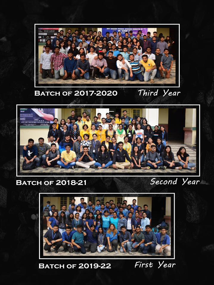


![college profile 2010-2011 - St. Xavier's College, Kolkata · 2020-02-28 · ST. XAVIER’S COLLEGE [AUTONOMOUS], KOLKATA Glimpses 2010-11 Workshop cum Training on SPSS for teachers](https://img.pdfslide.net/doc/110x75/5f4b8019151cf9557e783d03/college-profile-2010-2011-st-xaviers-college-kolkata-2020-02-28-st-xavieras.jpg)