MOBILE ORDER THEORY AS APPLIED TO

POLYCYCLIC AROMATIC HETEROCYCLES

THESIS

Presented to the Graduate Council of the

University of North;Texas in Partial

Fulfillment of the Requirements

For the Degree of

MASTER OF SCIENCE

By

Kristin A. Fletcher, B.S., B.A.

Denton, iTexas

August, 51997

3 T ?

St8( M o . -739£

MOBILE ORDER THEORY AS APPLIED TO

POLYCYCLIC AROMATIC HETEROCYCLES

THESIS

Presented to the Graduate Council of the

University of North;Texas in Partial

Fulfillment of the Requirements

For the Degree of

MASTER OF SCIENCE

By

Kristin A. Fletcher, B.S., B.A.

Denton, iTexas

August, 51997

3 T ?

St8( M o . -739£

toy

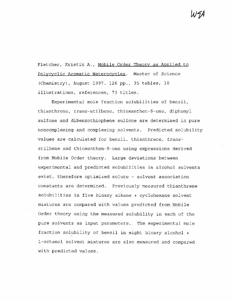
Fletcher, Kristin A., Mobile Order Theory as Applied to

Polvcvclic Aromatic Heterocvcles. Master of Science

(Chemistry), August 1997. 126 pp., 35 tables, 10

illustrations, references, 73 titles.

Experimental mole fraction solubilities of benzil,

thianthrene, fcrans-stilbene, thioxanthen-9-one, diphenyl

sulfone and dibenzothiophene sulfone are determined in pure

noncomplexing and complexing solvents. Predicted solubility

values are calculated for benzil, thianthrene, trans-

stilbene and thioxanthen-9-one using expressions derived

from Mobile Order theory. Large deviations between

experimental and predicted solubilities in alcohol solvents

exist, therefore optimized solute - solvent association

constants are determined. Previously measured thianthrene

solubilities in five binary alkane + cyclohexane solvent

mixtures are compared with values predicted from Mobile

Order theory using the measured solubility in each of the

pure solvents as input parameters. The experimental mole

fraction solubility of benzil in eight binary alcohol +

1-octanol solvent mixtures are also measured and compared

with predicted values.

ACKNOWLEDGMENTS

This work is dedicated to my research advisor, Dr.

William Acree, Jr. Without Dr. Acree's support and

encouragement, my goals would have been difficult to meet.

I would like to express my sincere gratitude for his

patience, time, advice and direction unselfishly given to me

during the course of my stay at the University of North

Texas.

I would like to thank Mary McHale, Joyce Powell, Karen

Coym, Carmen Hernandez, and Lindsay Roy for their help with

collecting data. And I would especially like to thank Sid

Pandey for his great support and belief in me.

Lastly, I would like to thank my mother and sister for

years of unconditional love and encouragement.

TABLE OF CONTENTS

Page

LIST OF TABLES . . vi

LIST OF ILLUSTRATIONS xi

Chapter

I. THE DEVELOPMENT OF MOBILE ORDER THEORY 1

Introduction '. . 1 Activity, Solubility and Chemical

Potential 9 Mobile Order Theory: Conceptual Basis. . . 14 Mobile Order Theory: Thermodynamic

Basis 19 Mobile Order Theory: Solute Solubility

in Pure Solvents 23 Mobile Order Theory: Solute Solubility

in Binary Alkane + Alcohol Solvent Mixtures 29

Mobile Order Theory: Solute Solubility in Binary Alcohol + Alcohol Solvent Mixtures 35

Chapter References 40

II. EXPERIMENTAL PROCEDURES AND RESULTS 44

Materials 44 Experimental Procedures and Results:

Pure Solvent Studies 45 Benzil Study in Pure Solvents 48 Thianthrene Study in Pure Solvents . . . .49 trans-Stilbene Study in Pure Solvents. . . 50 Thioxanthene-9-one Study in Pure

Solvents 51 Diphenyl Sulfone Study in Pure Solvents. . 52 Dibenzothiophene Sulfone Study in Pure

Solvents 52 Experimental Procedure: Binary Solvent

Studies 60 The Beer-Lambert Law 66 Chapter References 68

III. CONCLUSIONS AND DISCUSSIONS 69

Test for Binary Solvent Solubility Data Consistency 69

Results: Pure Solvent Studies 82 Results: Benzil Study 87 Results: Thianthrene Study 87 Results: trans-Stilbene Study 88 Results: Thioxanthen-9-one Study 89 Solute-Solvent Association Constants . . . 95 Solubility of Thianthrene in Binary

Alkane + Alkane Solvent Mixtures as Predicted by Mobile Order Theory. . .100

Results: Benzil in Binary Alcohol Solvents 104

Conclusions 109 Chapter References 113

APPENDIX: GLOSSARY 115

Terms 115 Symbols 118 Greek Letters 12 0

REFERENCES 122

LIST OF TABLES

Table _ Page I. Spectrochemical Solute Properties

used in Mobile Order Predictions 47

II. Experimental Benzil Mole Fraction Saturation Solubility in Select Nonelectrolyte Solvents at 25 °C 54

III. Experimental Mole Fraction Saturation Solubility of Thianthrene in Select Nonelectrolyte Solvents at 25 °C 55

IV. Experimental Mole Fraction Saturation Solubility of fcrans-Stilbene in Select Nonelectrolyte Solvents at 25 °C 56

V. Experimental Mole Fraction Saturation Solubility of Thioxanthen-9-one in Select Nonelectrolyte Solvents at 25 °C 57

VI. Experimental Mole Fraction Saturation Solubility of Diphenyl Sulfone in Select Nonelectrolyte Solvents at 25 °C 58

VII. Experimental Mole Fraction Saturation Solubility of Dibenzothiophene Sulfone in Select Nonelectrolyte Solvents at 25 °C . 59

VIII. Experimental Mole Fraction Solubilities of Benzil (X a ) in Binary 1-Propanol (B) + 1-Octanol (C) Solvent Mixtures at 25 °C 62

IX. Experimental Mole Fraction Solubilities of Benzil (X a ) in Binary 2-Propanol (B) + 1-Octanol (C) Solvent Mixtures at 25 °C 62

X. Experimental Mole Fraction Solubilities of Benzil (X^at) in Binary 1-Butanol (B) + 1-Octanol (C) Solvent Mixtures at 25 °C 63

XI. Experimental Mole Fraction Solubilities of Benzil (XA

at) in Binary 2-Butanol (B) + 1-Octanol (C) Solvent Mixtures at 25 °C 63

XII. Experimental Mole Fraction Solubilities cat"

of Benzil (XA ) in Binary 2-Methyl-1-Propanol (B) + 1-Octanol (C) Solvent Mixtures at 25 °C 64

XIII. Experimental Mole Fraction Solubilities c a t~

of Benzil (XA ) + 1-Octanol (C) 25 °C

in Binary 1-Pentanol (B) Solvent Mixtures at

64

XIV. Experimental Mole Fraction Solubilities of Benzil (XA ) in Binary 3-Methyl-l-Butanol (B) + 1-Octanol (C) Solvent Mixtures at 25 °C 65

XV. Experimental Mole Fraction Solubilities of Benzil (XA

at) in Binary 4-Methyl-2-Pentanol (B) + 1-Octanol (C) Solvent Mixtures at 25 °C 65

XVI. Mathematical Representation of Experimental Benzil Solubilities in Several Binary Alcohol (B) + 1-Octanol (C) Solvent Mixtures 73

XVII. Solvent Properties Used in Mobile Order Predictions 85

XVIII. Thermodynamic Solute Properties Used in Mobile Order Predictions 86

XIX. Comparison Between Experimental Benzil Mole Fraction Solubilities and Predicted Values Based upon Mobile Order Theory . . 91

XX. Comparison Between Experimental Thianthrene Mole Fraction Solubilities and Predicted Values Based Upon Mobile Order Theory 92

XXI. Comparison Between Experimental trans-Stilbene Mole Fraction Solubilities and Predicted Values Based Upon Mobile Order Theory 93

XXII

XXIII

XXIV.

XXV.

XXVI.

XXVII

XXVIII

XXIX.

XXX.

Comparison Between Experimental Thioxanthen-9-one Mole Fraction Solubilities and Predicted Values Based upon Mobile Order Theory 94

Optimized Association Constant for Benzil - Solvent Associations in Alcohol Solvents 98

Optimized Association Constant for Thioxanthen-9-one - Solvent Associations in Alcohol Solvents 99

S ct t 6XH)

Comparison of Experimental, (XA ) , versus Predicted, (XA

at)cac, Mole Fraction Solubilities of Thianthrene in Binary n-Hexane (B) + Cyclohexane (C) Solvent Mixtures at 25 °C 102

S S t OXT3 Comparison of Experimental, (X, ) , T-S -« • , ,- rsat vcalc

versus Predicted, (XA ) , Mole Fraction Solubilities of Thianthrene in Binary n-Heptane (B) + Cyclohexane (C) Solvent Mixtures at 25 °C 102

Comparison of Experimental, (XAat)exp,

versus Predicted, (XAat)cac, Mole

Fraction Solubilities of Thianthrene in Binary n-Octane (B) + Cyclohexane (C) Solvent Mixtures at 25 °C 103

Comparison of Experimental, (XAat)exp,

versus Predicted, (XAat)cac, Mole

Fraction Solubilities of Thianthrene in Binary Methylcyclohexane (B) + Cyclohexane (C) Solvent Mixtures at 25 °C 103

Comparison of Experimental, (XAat)exp,

versus Predicted, (XAat)ca c, Mole

Fraction Solubilities of Thianthrene in Binary Cyclooctane (B) + Cyclohexane (C) Solvent Mixtures at 25 °C 104

Comparison of Experimental, (XAat)exp,

versus Predicted, (XAat)cac, Mole

Fraction Solubilities of Benzil in Binary 1-Propanol (B) + 1-Octanol (C) Solvent Mixtures 106

XXXI

XXXII

XXXIII

XXXV.

Comparison of Experimental, (X^at

versus Predicted, (X^at)ca c, Mole Fraction Solubilities of Benzil Binary 2-Propanol (B) + 1-Octanol Solvent Mixtures

m

.sat Comparison of Experimental, (XA versus Predicted, (X^at)ca c, Mole Fraction Solubilities of Benzil Binary 1-Butanol (B) + 1-Octanol Solvent Mixtures

m

Comparison of Experimental, (X^at

versus Predicted, (X^at)cac, Mole Fraction Solubilities of Benzil Binary 2-Butanol (B) + 1-Octanol Solvent Mixtures

XXXIV. Comparison of Experimental •*! * * "*I / •• ScilIII \ CSt JL C versus Predicted, (XA )

rsat (*A Mole

Fraction Solubilities of Benzil in Binary 2-Methyl-1-Propanol (B) + 1-Octanol (C) Solvent Mixtures.

rsat

exp

(C)

exp

(C)

exp

in (C)

exp

exp Comparison of Experimental, (X versus Predicted, (X^at)cac, Mole Fraction Solubilities of Benzil in Binary 1-Pentanol (B) + 1-Octanol (C] Solvent Mixtures. ,

107

107

108

108

109

LIST OF ILLUSTRATIONS

Figure Page

1. Molecular Structures of Solutes Studied: (A) Benzil, (B) Thianthrene, (C) trans-Stilbene, (D) Thioxanthen-9-one, (E) Diphenyl Sulfone, (F) Dibenzothiphene Sulfone 6

2. Diagram of Single Chain Hydrogen Bonding Ensemble 16

3. Graphical Representation of Benzil in Binary 1-Propanol + 1-Octanol Solvent Mixtures. Solid Lines ( ) Represent Experimentally Determined Solubilities, and Dashed Lines ( ) Represent "Best Fit" Curves 74

4. Graphical Representation of Benzil in Binary 2-Propanol + 1-Octanol Solvent Mixtures. Solid Lines ( ) Represent Experimentally Determined Solubilities, and Dashed Lines ( ) Represent "Best Fit" Curves 75

5. Graphical Representation of Benzil in Binary 1-Butanol + 1-Octanol Solvent Mixtures. Solid Lines ( ) Represent Experimentally Determined Solubilities, and Dashed Lines ( ) Represent "Best Fit" Curves 7 6

6. Graphical Representation of Benzil in Binary 2-Butanol + 1-Octanol Solvent Mixtures. Solid Lines ( ) Represent Experimentally Determined Solubilities, and Dashed Lines ( ) Represent "Best Fit" Curves 77

7. Graphical Representation of Benzil in Binary 2-Methyl-l-Propanol + 1-Octanol Solvent Mixtures. Solid Lines ( ) Represent Experimentally Determined Solubilities, and Dashed Lines ( ) Represent "Best Fit" Curves 78

8. Graphical Representation of Benzil in Binary 1-Pentanol + 1-Octanol Solvent Mixtures. Solid Lines ( ) Represent Experinentally Determined Solubilities, and Dashed Lines ( ) Represent "Best Fit" Curves 79

9. Graphical Representation of Benzil in Binary 3-Methyl-1-Butanol + 1-Octanol Solvent Mixtures. Solid Lines ( ) Represent Experinentally Determined Solubilities, and Dashed Lines ( ) Represent "Best Fit" Curves 80

10. Graphical Representation of Benzil in Binary 4-Methyl-2-Pentanol + 1-Octanol Solvent Mixtures. Solid Lines ( ) Represent Experinentally Determined Solubilities, and Dashed Lines ( ) Represent "Best Fit" Curves 81

CHAPTER I

THE DEVELOPMENT OF MOBILE ORDER THEORY

Introduction

Since the turn of the century scientists have been

interested in understanding the behavior of solutions in

order to develop mathematical models capable of describing

both the specific and nonspecific interactions present in

polar and nonpolar solutions. More recently researchers

have been able to predict the solubility of select

crystalline organic nonelectrolyte solutes in organic

nonelectrolyte solvents with a great deal of accuracy from

group contribution methods and/or semi-empirical

mathematical representations of solution behavior.1 Group

contribution methods for predicting thermodynamic properties

of nonelectrolyte solutions do require a priori knowledge of

interactional parameters for the various functional groups

contained in the molecules. Unfortunately, there exist a

large number of common functional groups for which

2

parameters have yet to be determined. On the other hand,

the theory of Mobile Order developed by Huyskens, Ruelle and 3-13

coworkers has been shown to accurately predict the

solubilities of inert and select associating crystalline

2

solutes in pure, binary, and higher order mixtures of both

complexing and noncomplexing solvents. Also, Mobile Order

theory is the only thermodynamic model able to accurately

predict the solubility of inert crystalline solutes in

solvents containing alcohol-, ether-, alkoxy-, chloro-, and

alkane functional groups.

Solubility information can prove to be useful to many

different facets of science from biology to civil

engineering to pharmaceutical chemistry.14 In the chemical

industry, a thorough understanding of the thermodynamic and

physical properties of a multicomponent system is very

important for the design calculations involving chemical

separations, mass transfer, heat flow or fluid flow.

However, without mathematical models, the thermodynamic

information obtained from solubility and equilibria data is

of little use in many applications.15

Thermodynamic principles provide a mathematical

foundation for predicting unknown properties from measured

experimental or tabulated data. Thermodynamic properties

such as the partial vapor pressure or the kinetic behavior

of a substance dissolved in solution are determined to a

large extent by solute-solvent and solvent-solvent

interactions.16 Therefore, understanding how a solvent

behaves in solution is crucial to developing useful and

applicable solution theories. The goal of modern day

solution thermodynamicists is to develop predictive

3

equations capable of describing thermodynamic behavior in

complex, multicomponent systems from structural

considerations and pure component properties.

Continued development of models able to describe the

thermodynamic properties of nonelectrolyte solutions

requires that an extensive data base be readily available in

order to thoroughly examine the predictive ability,

limitations, and applications of such derived expressions.

Extensive studies into the thermodynamic properties of inert

solutes dissolved in pure and binary complexing and

noncomplexing systems have been conducted by the research

groups of Huyskens16'18, Acree19"34, and Ruelle.3,5'6'13,35"41

For the most part, the afore-mentioned studies examined the

solubility behavior of inert solutes dissolved in either

neat or binary solvent mixtures containing alkanes, aromatic

hydrocarbons and/or alcohols. Very few complexing solutes

were studied.

The purpose of my thesis research is to conduct a

preliminary study regarding the solubility behavior of

select polycyclic aromatic sulfur hetero-atoms (PASHs) and

oxygen-containing solutes in order to identify interesting

systems for future studies. Many of the predictive methods

that have been derived for describing solute solubility in

binary solvent mixtures require as input parameters the

measured solute solubility in both neat solvent components.

Of particular interest would be binary solvent mixtures in

4

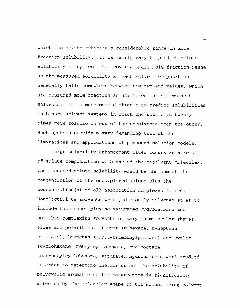
which the solute exhibits a considerable range in mole

fraction solubility. It is fairly easy to predict solute

solubility in systems that cover a small mole fraction range

as the measured solubility at each solvent composition

generally falls somewhere between the two end values, which

are measured mole fraction solubilities in the two neat

solvents. It is much more difficult to predict solubilities

in binary solvent systems in which the solute is twenty

times more soluble in one of the cosolvents than the other.

Such systems provide a very demanding test of the

limitations and applications of proposed solution models.

Large solubility enhancement often occurs as a result

of solute complexation with one of the cosolvent molecules.

The measured solute solubility would be the sum of the

concentration of the uncomplexed solute plus the

concentration(s) of all association complexes formed.

Nonelectrolyte solvents were judiciously selected so as to

include both noncomplexing saturated hydrocarbons and

possible complexing solvents of varying molecular shapes,

sizes and polarities. Linear (n-hexane, u-heptane,

n-octane), branched (2,2,4-trimethylpentane) and cyclic

(cyclohexane, methylcyclohexane, cyclooctane,

fcert-butylcyclohexane) saturated hydrocarbons were studied

in order to determine whether or not the solubility of

polycyclic aromatic sulfur heteroatoms is significantly

affected by the molecular shape of the solubilizing solvent

5

media. Molecules generally mix so as minimize void volume

and maximize favorable exothermic molecular interactions.

Inefficient molecular packing leads to larger void volumes,

and a reduced number of molecular contacts between

neighboring molecules. It is conceivable that certain

geometric solvent shapes may not be compatible with the

aromatic ring system contained in the PASH solutes.

Alcohol solvents were selected because of their

potential to form hydrogen bonds with solutes such as

benzil, thianthrene, thioxanthen-9-one, diphenyl sulfone,

and dibenzothiophene sulfone. The molecular structures of

these five solutes, along with trans-stilbene, are depicted

in Figure 1. Hydrogen bond formation could occur through

the lone pairs of electrons on the sulfur atoms in

thianthrene or through the lone pairs of electrons on the

oxygen atom and the two lone electron pairs on the sulfur

atom in thioxanthen-9-one. In the case of benzil, diphenyl

sulfone and dibenzothiophene sulfone, the oxygen atoms

provide two lone electron pairs for possible hydrogen bond

formation with the alcoholic OH groups. fcrans-Stilbene was

chosen because of the absence of functional groups, yet its

structure is similar to other solutes in the study. Data

for trans-stilbene will provide an indication of the general

trends in solubility, which will be needed to illustrate the

enhancement in solubility due to the hydrogen bonding

between solute and solvent molecules. The relative strength

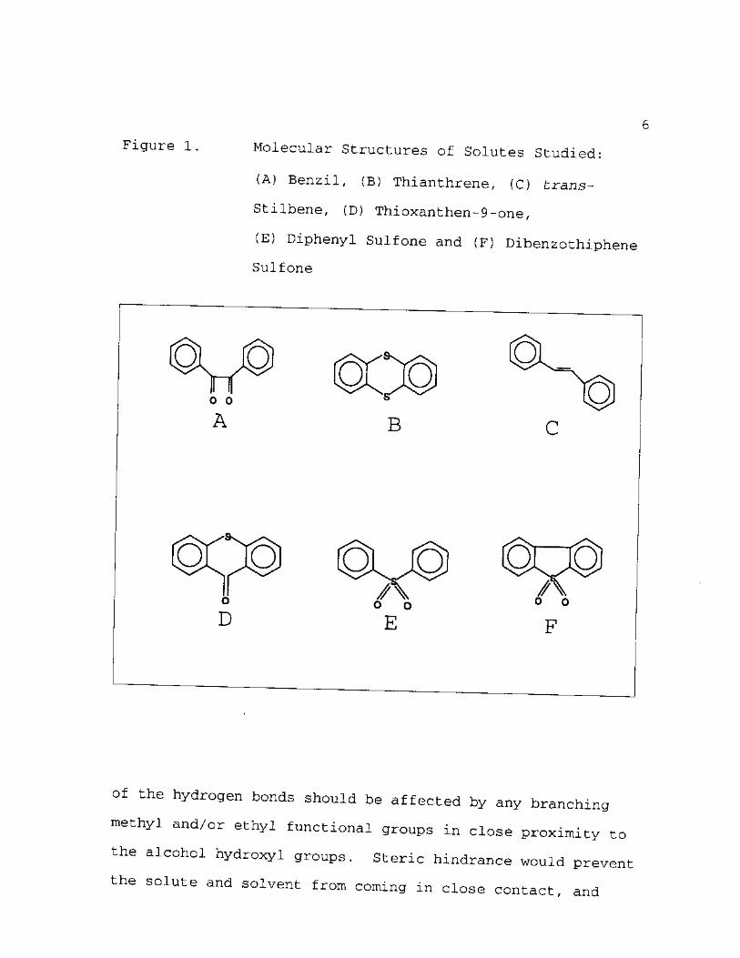
Figure 1 Molecular Structures of Solutes Studied:

Benzil, (B) Thianthrene, (C) trans—

Stilbene, (D) Thioxanthen-9-one,

(E) Diphenyl Sulfone and (F) Dibenzothiphene

Sulfone

of the hydrogen bonds should be affected by any branching

methyl and/or ethyl functional groups in close proximity to

the alcohol hydroxyl groups. Steric hindrance would prevent

the solute and solvent from coming in close contact, and

7

would thus lead to a weaker association complex. The

branched alcohol solvents studied have the methyl and/or

ethyl groups either immediately adjacent to hydroxyl group

(2-methyl-2-butanol, 2-methyl-1-pentanol, 2-ethyl-l-hexanol,

2-methyl-2-butanol), or not too far removed from the

hydroxyl group (3-methyl-l-butanol, 4-methyl-2-pentanol).

In order to assess the accuracy of the approximation of the

association constant, one needs to experimentally determine

the solute solubility in noncomplexing solvents such as

saturated n-alkanes, and also in highly nonideal solvents

like alcohols.

The failure of the previous theories to correctly

describe associated solutions may be attributed to the

incorrect view of the entropic nature of the hydrogen

bonding. In general, past models of solution behavior were

incapable of predicting the solubility of an inert

crystalline solute in highly nonideal systems. For the most

part the equations developed to predict solubility have

differed from each other in the method of approximating the

association constant of the various monomers, dimers,

trimers, etc., and also in the representation of the entropy

of mixing. By comparing the experimental solubilities in

both ideal and nonideal systems with predicted solubilities,

one may perhaps determine the weaknesses of that particular

solution model. With previous solution models, deviations

between predicted versus experimental solubilities increase

8

as the differences between solvent and solute molar volumes

increased. Solution theories based upon Raoult's law

repeatedly under-predicted the solubilities, while the

Flory-Huggins solution models over-predicted solubilities.

The incorrect assumption that the entropy of mixing can be

calculated using the Boltzmann equation for probability

becomes obvious when one compares predicted versus

experimental solubilities for systems whose solute-solvent

molar volumes differ from each other by more than a factor

of two. These discrepancies largely vanish when one

utilizes the equations developed for Mobile Order theory.

It is hoped that the information gained from the

solubility behavior of polycyclic aromatic hetero-atom

solutes in alcohol solvent systems will be extendable to

aqueous systems. Our planet is 7 0 per cent water, and the

solubility in aqueous systems controls, to a large extent, a

pollutant's toxicity to aquatic organisms, adsorption into

the soil and sediment, as well as the transfer to other

media. An understanding of the solute-solvent and solvent-

solvent interactions at the molecular level has

unfortunately not progressed to the point where it is

possible to predict the solubility of organic substances in

water from only structural considerations. For one thing,

water undergoes autoprotolysis (2H20 H30+ + OH~) and its

two hydrogen atoms are each capable of participating in

hydrogen bond formation. Studies involving monofunctional

9

alcohols reduce the number of solute-solvent and solvent-

solvent hydrogen bonds formed, and thus give simpler systems

to thermodynamically model.

It should also be noted that environmentally important

solutes were selected for study. PASHs have been shown to

exhibit enhanced bio-accumulation as compared to their

polycyclic aromatic hydrocarbon (PAH) counterparts and both

types of compounds exhibit mutagenic as well as carcenogenic

capabilities. PASHs are a concern in the petroleum industry

because they poison the catalysts used in desulfuration and

catalytic hydrocarbon cracking processes, and they also

produce toxic S02 vapor as well as additional sulfur-

2 containing pollutants.

A glossary of terms and symbols used throughout this

work is provided in the Appendix.

Activity, Solubility and Chemical Potential

The activity of a given state depends upon the

temperature, pressure, composition, and specific state

chosen. Therefore, unless there is a description of the

state chosen, the activity of component i loses its meaning.

The standard state activity is generally defined as unity,

and is typically one of two types: the symmetrical or the

unsymmetrical reference state.15,42 The symmetrical

reference state defines the standard state as the pure

10

liquid or pure solid at the temperature and pressure of the

system. The chemical potential of solute and solvent are

both defined in terms of their mole fraction compositions.

The unsymmetrical reference state distinguishes between the

solute and solvent. The solvent reference state is

described by Raoult's law, which states that the fugacity of

each component in a multicomponent system is equal to the

product of the mole fraction composition of the specified

component and the fugacity of the pure component at the

temperature of the system, and the activity is generally

15

expressed m terms of mole fraction. The solute reference

state, on the other hand, is generally defined in terms of

the properties of a hypothetical state, which is obtained by

extrapolating the measured solute properties at infinite

dilution to a 1 molar (or 1 molal) solution. The

unsymmetrical reference state is defined in the literature

as Henry's law, which states that for dilute systems the

solubility of a solute is directly proportional to its

partial pressure.15

The activity, aL, of a substance, i, is related to its

concentration through the activity coefficient, Yi

= YiXi (eq 1.1)

where Yi is the mole fraction activity coefficient, and Xi

is the mole fraction of component i.15,42 The activity of

11

the solute can be related to the chemical potential, ui# by

43 the following thermodynamic relation

UA " % = RT lnaflld (eq 1.2)

By suitable mathematical manipulations, one may relate a

solute's solubility to its chemical potential, and thus the

partial molar excess Gibbs free energy of mixing of the

solute:43

AGf = RT In(a^olid/X^at) (eq 1.3)

as defined in terms of the gas constant, R, the temperature

of the system under study, T, the activity of the solid

solute, a^olld , and the saturation mole fraction solubility

of the solute, X^at. This equation corresponds to Raoult's

law, and the mole fraction version of solubility and Gibbs

free energy. The Flory-Huggins description of the solute's

partial molar excess Gibbs energy can be expressed in terms

of the volume fraction solubility, cf)^,44

AGf = RT[ln(arlid/Ct) " (1 " V°/Vs)] (eq 1.4)

The molar volume of the solute and solvent are denoted as

and Vs, respectively. Once the partial molar Gibbs energy

12

of mixing is known, one may calculate other partial molar

thermodynamic properties by differentiating AGmix in the

proper fashion.45

A solution can be considered ideal if the change in

enthalpy, internal energy, volume, constant pressure heat

capacity, and constant volume heat capacity are zero upon

mixing of pure components. The chemical potential of each

species in solution, Ta±, can be represented by its standard

chemical potential, p°, and its mole fraction solubility,

Xj by the following relationship42

Pi = u°(T,P) + RTln (XA) (eg 1.5)

In the case of a crystalline nonelectrolyte solute,

activity is equivalent to its ideal mole fraction

solubility, (a"01")" = (xfV 1.

n / solid, id , , sat__satNid ln(aA ) = LN(YA XA )

= - AH^PS (TTP - T) (RTTTP)_1 + ACP(TTP - T) (RT)"1

- ACpln(TTp/T)R 1 (eg 1.6)

Ideal solubility is calculated from the solute's heat of

fusion, AH^pS, its triple point temperature, Ttp, its heat

capacity at constant pressure, ACp, and the temperature of

44 the system, T. For an ideal solution, the activity

13

coefficient of the solute, Ya^' unity. Thus, the

activity coefficient plays a crucial role in determining the

total nonideality of a system, as it reflects the relative

strengths of the intermolecular forces between the different

components in the solution, i.e. van der Waals forces,

London dispersion forces, dipole-dipole interactions, and

hydrogen bonding. Understanding the role of specific and

nonspecific interactions aids in the determination of the

total nonideality of the system under investigation. This

is especially true when one attempts to distinguish between

complexation and preferential solvation in the presence of

weak association complexes.46 The excess properties of a

solute near infinite dilution: the change in the Gibbs free

energy, enthalpy, entropy, volume, etc. upon mixing, can

provide very useful information into both the causes and

4 2

effects of solution nonideality.

There are two general reasons for solution nonideality:

physical effects and chemical effects. The physical effects

result from a random distribution of the components in

solution, and chemical deviations arise as a result of the

specific geometric orientations of one molecule with respect

to other species in solution. In nonassociating systems,

the classical physical solution models adequately predict

solution behavior. However, as the system moves further

from an ideal situation, the predictive ability of the

classical theories steadily decreases. On the other hand,

14

theories that attribute all solution nonideality to the

formation of molecular complexes and completely disregard

the effects of nonspecific interactions require several

equilibrium constants and complicated mathematical

relationships to accurately describe the enhancement of the

experimental solubility of a solute dissolved in pure self-

associating solvents. When strong specific interactions are

present in solution, models which include molecular

complexes are able to predict solubility data quite well,

however, one needs to properly account for the nonspecific

interactions that are always present.

Mobile Order Theory: Conceptual Basis

Traditional expressions derived to predict the

solubility of an inert crystalline solute dissolved in

associating solvents assumed the solution was ergodic, or

that the fraction of molecules involved in hydrogen bonding

is equivalent to the fraction of time a given molecule is

involved in a hydrogen bond with a neighboring molecule. If

one assumes self-associating liquids behave in an ergodic

manner, the thermodynamic probability of atom X being

associated with another molecule is calculated from the

surface fraction of atom X. It can be shown that

amphiphilic solvents, solvents that possess a proton donor

and proton acceptor site, deviate strongly from this

15

assumption.16,18'47 For example, for an alcohol solvent the

hydroxyl proton follows a neighboring oxygen atom 95% of the

time, which is significantly greater than the fraction of

time this association was predicted to occur based upon

classical interpretations of ensemble fractions. The

nonergodic behavior of associating solutions was first put

forth by Huyskens and Haulait-Pirson.16 From this new

assumption of solution behavior they, along with Ruelle and

coworkers, have developed the theory of Mobile Order which

can accurately predict the solubility of an inert solute

dissolved in associating or nonassociating solvents.3 13,48

The nonergodic behavior of alcoholic solvents arises

from the fact that each hydroxy group possess three sites

for hydrogen bonding: one hydroxyl proton and two lone pairs

of electrons on the oxygen atom. The proton may be free of

a hydrogen bond, yet a lone pair of electrons can still bind

the oxygen in a H-bond. Therefore, hydrogen bond ensembles

resembling Figure 2 can form in solution.10 For simplicity,

it is assumed that only the first electron donor site of the

oxygen atom forms a hydrogen bond, and no branching in the

chain occurs. This assumption is supported by experimental

evidence showing the second hydrogen bond is much weaker

after the formation of a first bond if the bonds are formed

in the same manner, i.e. hydrogen bonds of two proton

acceptors or two proton donors.10,12,16'47 If ergodic

behavior is assumed, then only those molecules completely

16

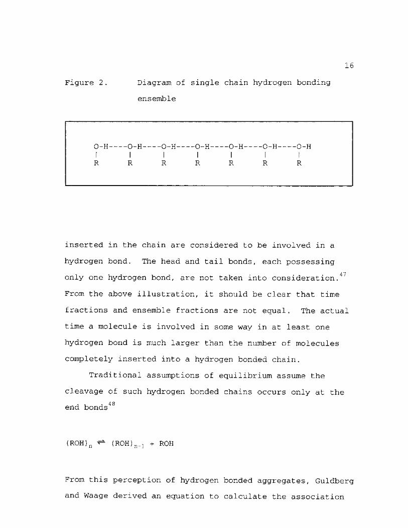
Figure 2. Diagram of single chain hydrogen bonding

ensemble

0-H--I

—0-H— I I I I i

--0-H I 1

R 1 R

1 R

1 R

1 R

1 R

1 R

inserted in the chain are considered to be involved in a

hydrogen bond. The head and tail bonds, each possessing

only one hydrogen bond, are not taken into consideration.47

From the above illustration, it should be clear that time

fractions and ensemble fractions are not equal. The actual

time a molecule is involved in some way in at least one

hydrogen bond is much larger than the number of molecules

completely inserted into a hydrogen bonded chain.

Traditional assumptions of equilibrium assume the

cleavage of such hydrogen bonded chains occurs only at the

end bonds48

(ROH) n ^ (ROH)n_1 + ROH

From this perception of hydrogen bonded aggregates, Guldberg

and Waage derived an equation to calculate the association

17

constant, KA, of the various monomers, dimers, trimers, etc.

that are formed12

KA = [ (ROH)N] / [ (ROH)^] [ROH] (eq 1.7)

Or, to relate the association constant to the formal

concentration of the alcohol, CA, one may employ the

12 following relation

(an) / {an_x) (c ) = n/ (n-l)KACA (eq 1.8)

where an represents the fraction of molecules involved in

the chain depicted in Figure 2.

In order to properly account for the nonergodic nature

of self-associating solvents, one must calculate the

association constant, or more appropriately the insertion

constant, using time fractions instead of the ensemble

fractions of Guldberg and Waage.

(Y ~ L)/Y = KACa (eq 1.9)

or,

Y = [ 1 + K AC a ] 1 (eq 1.10 )

For single chains without branching, the insertion constant,

18

Ka, is related to the formal molar concentration of

associating species, CA, and to the probability in time that

an alcohol is free from hydrogen bonding, y. 7' 1 0' 4 7 jf the

alcohol is at high dilution or in nonassociating solvents, y

is approximately unity, and time fractions are approximately

50

equal to ensemble fractions. This explains the apparent

accuracy of classical predictions of the thermodynamic

properties of dilute systems.

The cleavage of such hydrogen bonded aggregates occurs

randomly, so one cannot assume only the end hydrogen bond is

broken. A more realistic depiction of the equilibrium of

the various i-mers of the hydrogen bonded liquids might take

the form of48

(ROH) g ^ (ROH) m + (ROH) n

where q = m + n. It can be shown that equations 1.9 and

1.10 accurately describe solution behavior regardless of

where the hydrogen bond is broken.

In solution, the disorder created from mixing two

liquids or a liquid and solid takes on a hybrid form:

possessing a static nature and a mobile nature. The static

disorder is accounted for by calculating the average number

of molecules of X that will be displaced by molecule Y, and

is ruled by the number of molecules of X added. The mobile

disorder is characterized by the fact that molecules are

19

permitted to travel freely through their domain. In order

to increase the domain available to a molecule Y, one needs

to introduce a foreign molecule X to the system. Therefore,

the mobile disorder of a solution is governed by the volume

of molecules of X added.

In order to mathematically account for the dual nature

of the entropy of mixing in liquids, both the mole fraction

and volume fraction of the added solute need to be

considered. The general expression for the entropy of

• • . 4 8

mixing is

A mix = -R.[nAln(XA 'c})A) + nglnfXg1 a><}>g) ] (eq 1.11)

where the classical expression for the entropy of mixing

based on Raoult's law corresponds to a = 0; a = 1

corresponds to the Flory-Huggins definition of the entropy

of mixing, and a = 1/2 was derived by Huyskens and Haulait-

Pirson. The differences between these three definitions for

the entropy of mixing only become apparent when there is a

significant difference in the solute and solvent molar

volumes.

Mobile Order Theory: Thermodynamic Basis

Classical solution thermodynamicists viewed the

dissolution of an inert crystalline solute into a hydrogen

20

bonded solvent as depending upon three main factors: the

breaking up of the solvent-solvent hydrogen bonds in order

to create a cavity large enough for the solute to reside,

the breaking up of the solute-solute cohesive forces so that

the solute may mix with the solvent, and the forming of

solute-solvent cohesive bonds, or if appropriate, hydrogen

15 44

bonds. ' This approach considers liquids as disordered

crystals, and completely ignores the continuous motions of

the molecules. In fact, there is no need to create a cavity

in which the solute will reside, the solvent molecules are

quite capable of moving around the solute without breaking

their hydrogen bonds and therefore without losing much of SO

the order of the system.

In systems capable of specific interactions between

solute-solute, solute-solvent and solvent-solvent molecules,

the correlation of the motions of the atoms in solution

brings a kind of order to the system and therefore reduces

the entropy. The order created is not static in nature, but

rather it is a dynamic ordering in that all of the hydrogen

bonded molecules in solution are perpetually changing

partners. To better visualize the situation present in

solution one may consider a given molecule as occupying a

given domain, DomA, whose neighbors perpetually change.

This is a mobile domain with its position in solution

continuously changing, but the average volume of said domain

has a well defined value equal to the volume one solvent

21

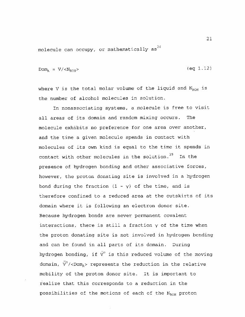
24 molecule can occupy, or mathematically as

DomA = V/<Nroh> (eq 1.12)

where V is the total molar volume of the liquid and NR0H is

the number of alcohol molecules in solution.

In nonassociating systems, a molecule is free to visit

all areas of its domain and random mixing occurs. The

molecule exhibits no preference for one area over another,

and the time a given molecule spends in contact with

molecules of its own kind is equal to the time it spends in

39

contact with other molecules in the solution. In the

presence of hydrogen bonding and other associative forces,

however, the proton donating site is involved in a hydrogen

bond during the fraction (1 - y) of the time, and is

therefore confined to a reduced area at the outskirts of its

domain where it is following an electron donor site.

Because hydrogen bonds are never permanent covalent

interactions, there is still a fraction y of the time when

the proton donating site is not involved in hydrogen bonding

and can be found in all parts of its domain. During

hydrogen bonding, if V° is this reduced volume of the moving

domain, V°/<DomA> represents the reduction in the relative

mobility of the proton donor site. It is important to

realize that this corresponds to a reduction in the

possibilities of the motions of each of the NR0H proton

22

donor sites and not a reduction in the possibilities of the

location of these molecules within the solution.

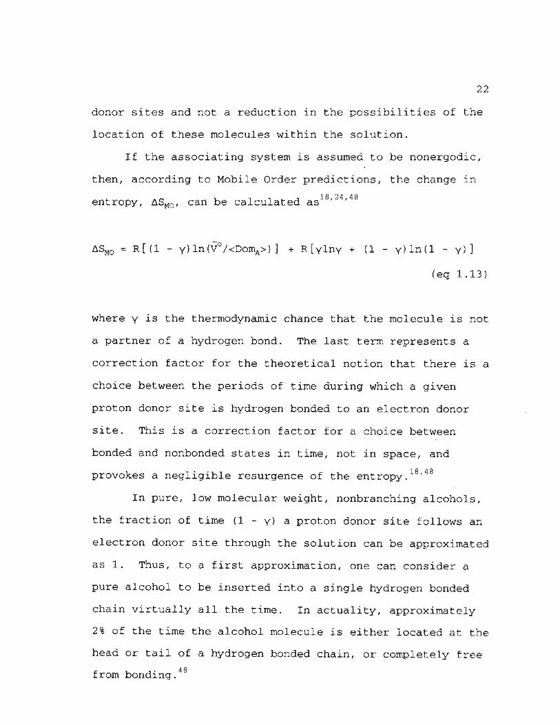
If the associating system is assumed to be nonergodic,

then, according to Mobile Order predictions, the change in

entropy, ASM0, can be calculated as18,24'48

AS m o = R [ ( l - y) ln(V°/<DomA>) ] + R [ y l n Y + (1 - y)ln(l - y) ]

(eq 1.13)

where y is the thermodynamic chance that the molecule is not

a partner of a hydrogen bond. The last term represents a

correction factor for the theoretical notion that there is a

choice between the periods of time during which a given

proton donor site is hydrogen bonded to an electron donor

site. This is a correction factor for a choice between

bonded and nonbonded states in time, not in space, and

provokes a negligible resurgence of the entropy.18,48

In pure, low molecular weight, nonbranching alcohols,

the fraction of time (1 - y) a proton donor site follows an

electron donor site through the solution can be approximated

as 1. Thus, to a first approximation, one can consider a

pure alcohol to be inserted into a single hydrogen bonded

chain virtually all the time. In actuality, approximately

2% of the time the alcohol molecule is either located at the

head or tail of a hydrogen bonded chain, or completely free

4 8 from bonding.

23

Contrary to traditional beliefs, the addition of a

small amount of inert substance does not significantly

decrease the fraction (1 - y) of alcohol molecules involved

in hydrogen bonding. In fact, the solute introduced into

solution does not alter V° at all, but rather increases the

mobile domain of the proton donor by virtue of the fact that

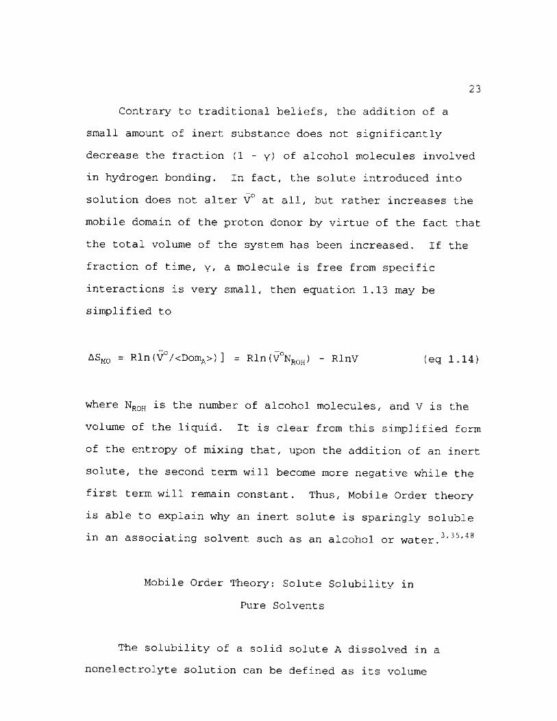
the total volume of the system has been increased. If the

fraction of time, y, a molecule is free from specific

interactions is very small, then equation 1.13 may be

simplified to

ASmo = Rln(V°/<DomA>) ] = Rln(V°NR0H) - RlnV (eg 1.14)

where NR0H is the number of alcohol molecules, and V is the

volume of the liquid. It is clear from this simplified form

of the entropy of mixing that, upon the addition of an inert

solute, the second term will become more negative while the

first term will remain constant. Thus, Mobile Order theory

is able to explain why an inert solute is sparingly soluble

in an associating solvent such as an alcohol or water.3,35'48

Mobile Order Theory: Solute Solubility in

Pure Solvents

The solubility of a solid solute A dissolved in a

nonelectrolyte solution can be defined as its volume

24

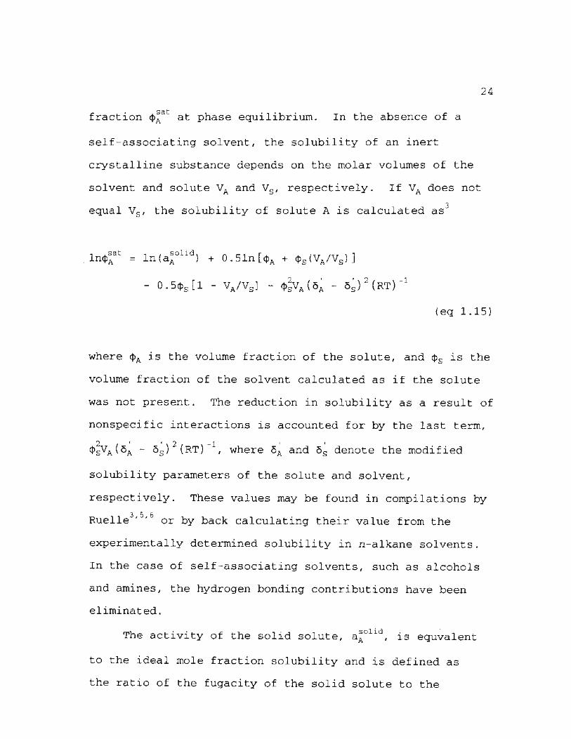
fraction c}>Aat at phase equilibrium. In the absence of a

self-associating solvent/ the solubility of an inert

crystalline substance depends on the molar volumes of the

solvent and solute VA and Vs, respectively. If VA does not

3 equal Vs, the solubility of solute A is calculated as

lnc|>Aat = ln(aA°

lid) + 0.51n[<()A + <f>s(VA/Vs)]

- 0.5<(>s[l - VA/VS] - 4>sVa(5a - 5S)2 (RT) 1

(eq 1.15)

where <j)A is the volume fraction of the solute, and <J>S is the

volume fraction of the solvent calculated as if the solute

was not present. The reduction in solubility as a result of

nonspecific interactions is accounted for by the last term,

2 i i 2 1 *

$sVA (5A - 5S) (RT) , where 5A and 5S denote the modified

solubility parameters of the solute and solvent,

respectively. These values may be found in compilations by

Ruelle3'J'6 or by back calculating their value from the

experimentally determined solubility in n-alkane solvents.

In the case of self-associating solvents, such as alcohols

and amines, the hydrogen bonding contributions have been

eliminated.

The activity of the solid solute, aAolld, is equvalent

to the ideal mole fraction solubility and is defined as

the ratio of the fugacity of the solid solute to the

25

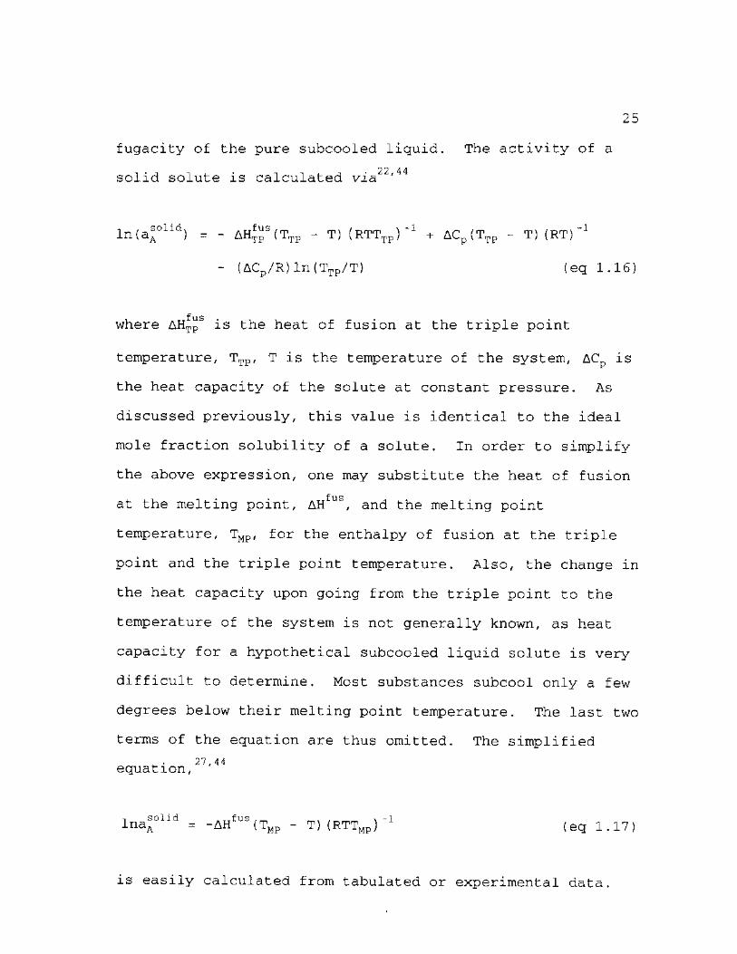
fugacity of the pure subcooled liquid. The activity of a

solid solute is calculated via22'44

In (a^°lid) = - AHTPS(Ttp - T) (RTTtp) _1 + ACp(TTP - T) ( R T ) " 1

- (ACp/R) In ( T t p / T ) (eq 1.16)

f U.S • where AHTP is the heat of fusion at the triple point

temperature, Ttp, T is the temperature of the system, ACp is

the heat capacity of the solute at constant pressure. As

discussed previously, this value is identical to the ideal

mole fraction solubility of a solute. In order to simplify

the above expression, one may substitute the heat of fusion

at the melting point, AHfus, and the melting point

temperature, TMP, for the enthalpy of fusion at the triple

point and the triple point temperature. Also, the change in

the heat capacity upon going from the triple point to the

temperature of the system is not generally known, as heat

capacity for a hypothetical subcooled liquid solute is very

difficult to determine. Most substances subcool only a few

degrees below their melting point temperature. The last two

terms of the equation are thus omitted. The simplified

2 7 , 44 equation,

lna®olld = -AHfus(TMp - T) (RTTMp) 1 (eq 1.17)

is easily calculated from tabulated or experimental data

26

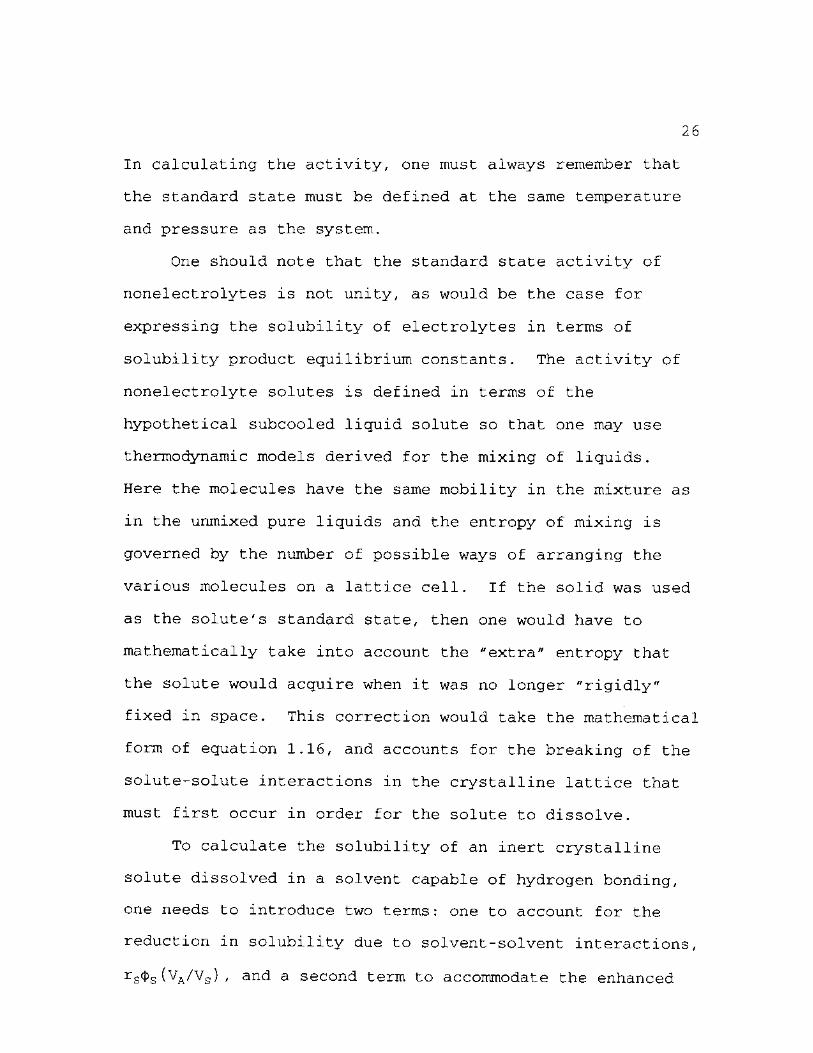
In calculating the activity, one must always remember that

the standard state must be defined at the same temperature

and pressure as the system.

One should note that the standard state activity of

nonelectrolytes is not unity, as would be the case for

expressing the solubility of electrolytes in terms of

solubility product equilibrium constants. The activity of

nonelectrolyte solutes is defined in terms of the

hypothetical subcooled liquid solute so that one may use

thermodynamic models derived for the mixing of liquids.

Here the molecules have the same mobility in the mixture as

in the unmixed pure liquids and the entropy of mixing is

governed by the number of possible ways of arranging the

various molecules on a lattice cell. If the solid was used

as the solute's standard state, then one would have to

mathematically take into account the "extra" entropy that

the solute would acquire when it was no longer "rigidly"

fixed in space. This correction would take the mathematical

form of equation 1.16, and accounts for the breaking of the

solute-solute interactions in the crystalline lattice that

must first occur in order for the solute to dissolve.

To calculate the solubility of an inert crystalline

solute dissolved in a solvent capable of hydrogen bonding,

one needs to introduce two terms: one to account for the

reduction in solubility due to solvent-solvent interactions,

rs<t>s(VA/Vs) , and a second term to accommodate the enhanced

27

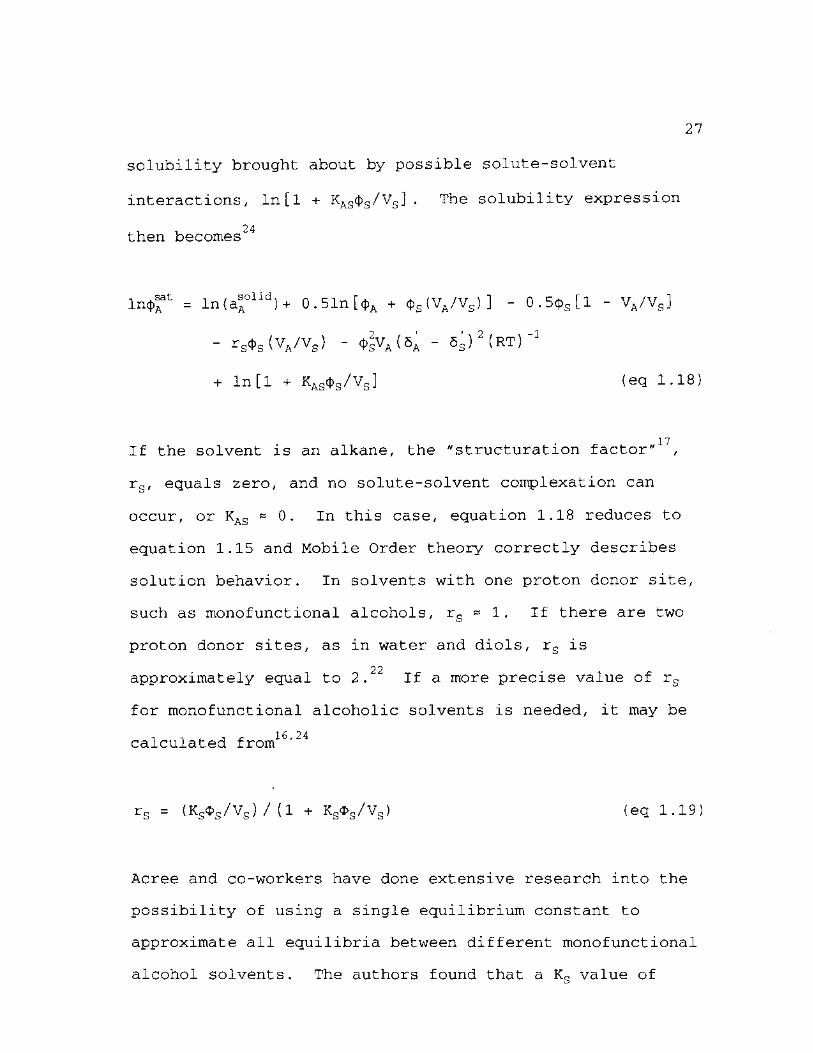
solubility brought about by possible solute-solvent

interactions, ln[l + KAS«|>S/VS] . The solubility expression

then becomes24

lncf) t = ln(aA° 1 )+ 0.51n[cj)A + <f»s(VA/Vs)] - 0.5$s[l - VA/VS]

" rs<Os(VA/Vs) - 4>sVa(5a " 5s)2(RT)_1

+ In [ 1 + Kasc))s/Vs] (eg 1.18)

17

If the solvent is an alkane, the "structuration factor" ,

rs, equals zero, and no solute-solvent complexation can

occur, or KAS « 0. In this case, equation 1.18 reduces to

equation 1.15 and Mobile Order theory correctly describes

solution behavior. In solvents with one proton donor site,

such as monofunctional alcohols, rs * 1. If there are two

proton donor sites, as in water and diols, rs is 22

approximately equal to 2 . If a more precise value of rs

for monofunctional alcoholic solvents is needed, it may be

calculated from16,24

rs = (Ks4>s/Vs) / (1 + Ks$s/vs) (eq 1.191

Acree and co-workers have done extensive research into the

possibility of using a single equilibrium constant to

approximate all equilibria between different monofunctional

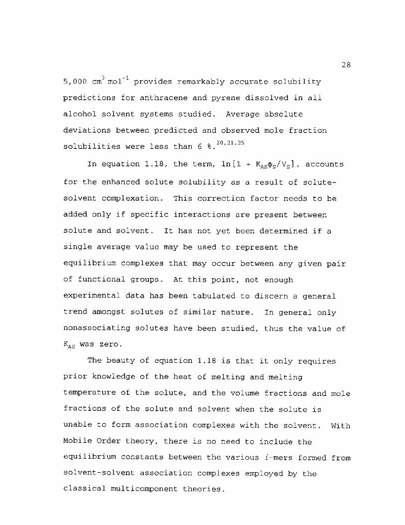
alcohol solvents. The authors found that a Ks value of

28

3 -1 5,000 cm mol provides remarkably accurate solubility

predictions for anthracene and pyrene dissolved in all

alcohol solvent systems studied. Average absolute

deviations between predicted and observed mole fraction

solubilities were less than 6 %-20'21'25

In equation 1.18, the term, ln[l + K A S c | > s / v S3 , accounts

for the enhanced solute solubility as a result of solute-

solvent complexation. This correction factor needs to be

added only if specific interactions are present between

solute and solvent. It has not yet been determined if a

single average value may be used to represent the

equilibrium complexes that may occur between any given pair

of functional groups. At this point, not enough

experimental data has been tabulated to discern a general

trend amongst solutes of similar nature. In general only

nonassociating solutes have been studied, thus the value of

Kas was zero.

The beauty of equation 1.18 is that it only requires

prior knowledge of the heat of melting and melting

temperature of the solute, and the volume fractions and mole

fractions of the solute and solvent when the solute is

unable to form association complexes with the solvent. With

Mobile Order theory, there is no need to include the

equilibrium constants between the various i-mers formed from

solvent-solvent association complexes employed by the

classical multicomponent theories.

2 9

Mobile Order Theory: Solute Solubility in

Binary Alkane + Alcohol Solvent Mixtures

The Gibbs energy of mixing for a system containing an

inert crystalline solid (A) dissolved in a binary alkane (B)

and alcohol (C) solvent mixture can be separated into three

contributions:

A G m i x = A G c o n f + A G c h e m + A G p h y s < e c3 1 - 2 0 )

where AGconf describes the configurational entropy, AGchem

represents the formation of hydrogen-bonded complexes, and

AGphyS results from weak nonspecific physical interactions

present in solution.

The configurational entropy is based upon the Huyskens

and Haulait-Pirson definition of solution ideality51

AGconf = 0. 5RT [nAlncf)A + nBln<t>B + ncln(J>c + nAlnXA + nBlnXc

+ n c lnX c ] (eg 1 .21)

The chemical contribution depends upon the

characteristics of the self-associating component, or

components, as well as the functional groups present. When

the interactions between molecules in solution result in the

specific orientation of one molecule with respect to other

molecules significant chemical contributions exist.44 The

30

most important chemical contributions that need to be

accounted for are those resulting from hydrogen bond

formation. For the present discussion I will consider the

hydrogen bonding between alcohols. As mentioned previously,

the number of available sites of hydrogen bonding on a

monofunctional alcohol is three, and the maximum number of

hydrogen bonds is limited by the donor or acceptor sites in

the minority.

Monofunctional alcohols are capable of forming

homogeneous, C-C, associated complexes. In the case of one

alcohol cosolvent, the fraction of time it is free from

22 hydrogen bonding, Ych:' -s given by

Ych: = [1 + Kc(J>c/vc] 1 (eg 1.22)

As predicted by the theory of Mobile Order, the chemical

contribution controlled by specific interactions between

molecules is52

AGchem = ncRTln [ (1 + Kc/vc)/(l + KccJ>c/Vc) ] (eq 1.23)

The physical contributions to the Gibbs energy of

mixing, such as London dispersion or van der Waals forces,

are accounted for by using the Nearly Ideal Binary Solvent

(NIBS) model developed by Bertrand, Burchfield, and

53-5 5 Acree which describes the solution behavior of a solute

31

dissolved in a binary solvent mixture incapable of forming

association complexes.

AGphys ~ (nA AnB B- AB + nA^AnC^C^AC + nB^BnC^C^BC)

x(nAVA + nBVB + ncVc) (eq 1.24)

The generalized weighting factors, r^, in the original

development have been approximated by the molar volumes of

each component, and is a binary interaction

parameter assumed to be independent of composition. Rarely

do real mixtures obey equation 1.24 , but instead the

terms display a slight compositional dependence. Binary

interactional parameters are related to modified solubility

parameters as follows:56

Aij = (5i - 5j)2 (eq 1.25)

By combining equations 1.21, 1.23 and 1.24, the molar

Gibbs energy of mixing is expressed as:

^ mix = 0 • 5RT [ XAlnc|)A + XBlncJ)B + X(-.ln0£ + XAlnXA + XBlnXB

+ XclnXc] + XcRTln [ (1 + Kc/Vc)/(1 + Kcc{>c/Vc]

+ ( XaVaXbVbAab + XaVaXcVcAac + XbVbXcVcAbc )

x (XAVA + XBVB + Xcvc) (eq 1.26)

Acree and Zvaigzne have been instrumental in developing

32

a predictive equation for the volume fraction saturation

solubility, <{>Aat, °f a n inert crystalline solute (A)

dissolved in a binary alkane (B) + alcohol (C) solvent

. . 20,22,24,57 mixture.

RT{ In ( a A °l l d / - 0.5 [1 - VA/ (X°VB + X°VC) ]

+ 0 .51n [VA/ (XgVB + X°VC)]

" (VA/VC) (Kc<t)c/Vc)0°(l + K^c/Vc)"1}

= Va[C(>b(5a - 5 g ) 2 + 4>°(5a - 5,1)2 - <t>°<|>°(5; - S ^ ) 2 ]

(eq 1.27)

where aAolld is the activity of the solid solute, 0°, XB, VB,

4>c' xc' a n d vc a r e t h e volume fractions, the mole fractions

and molar volumes of solvent B and C, respectively. The

volume and mole fractions B and C refer to the initial

binary solvent compositions calculated as if the solute were

not present. The modified solubility parameters for the

solute, alkane, and alcohol cosolvents are denoted as 5A,

5b, and 5C, respectively. Equation 1.27 is valid only in

the limit of sufficiently low solubility so that

1 - <t>®at « 1.0.

In order to reduce the complexity of the calculations

and improve the predictive capability of Mobile Order

theory, the terms containing the modified solubility

33

» '2 ' '2 parameter for the solute, (5A - 5B) and (5A - 5C) , may be

. 20 24 removed from equation 1.27 via '

V a ( 5 a - 5 b ) 2 = RT{ln[aAolid/(c()Aat)B] - 0 . 5 [1 - V A / V B ]

+ 0 .51n (VA/VB) } (eg 1.28)

and

V a ( 5 a - 5(1)2 = RT{ln[aAolid/(cf)Aat)c] - 0.5[1 - V A / V C ]

+ 0 . 51n (VA/VC) - (VAKC/V2)/(1 +KC/VC) }

(eq 1.29)

where (<t>Aat)B and (<t>A

at)c are the solubility of the solute in

the two pure solvents, B and C, respectively. Performing

the afore-mentioned substitutions and simplifying the

resulting equation, Acree and Zvaigzne obtained the

f TT . 20,22,25,57 following expression

ln<t>Aat = <t>Bln ( ) B + O X o D c " 0 . 5 [In (XBVB + X°VC)

- ct>BlnVB - (j>£lnVc] + (VaKc<J)°/V2) (1 + K c / V c )

_ 1

- (VaKcC|)°/V2) (1 + <t>cKc/Vc)

_ 1 + VAd)°(J)°(5B - 5 c ) 2 ( R T ) " 1

(eq 1.30)

for the volume fraction saturation solubility of an inert

solute dissolved in a binary alkane - alcohol mixture which

34

requires only a prior knowledge of the solute's solubility

in both pure solvents, values for the volume and mole

fractions of the two solvents, and the numerical value of

the alcohol's hydrogen-bond stability constant, Kc.

Careful examination of equation 1.3 0 reveals that the

predictive expression does correctly predict the

experimental solubility in both pure solvents. This would

' '2 ' '2 not be the case, however, if the (5A - 5B) and (5A - 5C)

terms remained in the final derived predictive expression.

The solute's modified solubility parameter would have to

somehow be calculated from the measured solute solubility

data. Mobile Order theory is not perfect, not even for

simple systems which are known to contain only nonspecific

interactions. The calculated numerical value of 5A would

vary slightly from one hydrocarbon cosolvent to another.

For example, in the case of trans-stilbene, one would

calculate numerical values of 5A = 19.78 MPa1/2,

5a = 19.68 MPa1/2, 5a = 19.60 MPa

1/2, using equation 1.3 0 and

the measured trans-stilbene solubilities in n-hexane,

n-heptane, and n-octane, respectively. Computations are

discussed in greater detail in Chapter 3.

Acree and coworkers have investigated the solubility of

pyrene and anthracene in 21 and 30 different binary alkane +

alcohol solvent systems, respectively. 20,24'31 Equation 1.3 0

was able to accurately predict the solubility of both

35

solutes to within an overall absolute average deviation of

less than 5 per cent using a single numerical value of

3 - 1

5,000 cm mol for the association constant of the five

alcohol cosolvents (1-propanol, 2-propanol, 1-butanol,

2-butanol and 1-octanol) studied. The authors further

showed that the predictive accuracy of Mobile Order theory-

was comparable to, and sometimes superior than, expressions

derived from the more conventional Kretschmer-Wiebe and 15

Mecke-Kempter association models. These latter two models

treat hydrogen-bonding in terms of discrete association

complexes, with concentrations of the various molecular

complexes formed being governed by the traditional notions

of equilibrium

ROH + (ROH)i ^ (ROH)i+1

The success of Mobile Order theory becomes more remarkable

when one considers that these particular systems are highly

nonideal. The ideal mole fraction solubility is calculated

to be 0.1312 and 0.01049 for pyrene and anthracene,

respectively, regardless of the solvent composition.58

Mobile Order Theory: Solute Solubility in

Binary Alcohol + Alcohol Solvents

In binary alcohol - alcohol solvent systems, the Gibbs

energy of mixing is again expressed as

36

59

AGmix - AGconf + AGchem + AGphys < e<3 1 • 31)

The configurational and physical contributions to the

energy of mixing are identical to the binary alkane +

alcohol systems developed in the previous section. However,

the chemical contribution significantly changes as a result

of additional heterogeneous associations between the two

alcohol cosolvents that were not possible in the presence of

one alcohol solvent. For each alcohol present in the

mixture, the fraction of time it is free from hydrogen

5 9 bonding, YBh: a n^ Ych:' given by

Y s h : — [ 1 + K b<|>B/VB + ( e q 1 . 3 2 )

and

Ych: — t + KqcJ^/Vq + Kcb(J)b/Vb] (eq 1.33)

where KBC and KCB denote the additional equilibrium constants

necessary to properly describe the formation of

heterogeneous alcohol association species not present in

pure the solvents. As predicted by the theory of Mobile

Order, the chemical contribution to the Gibbs free energy of

mixing controlled by specific interactions between solvents

B and C is

37

52

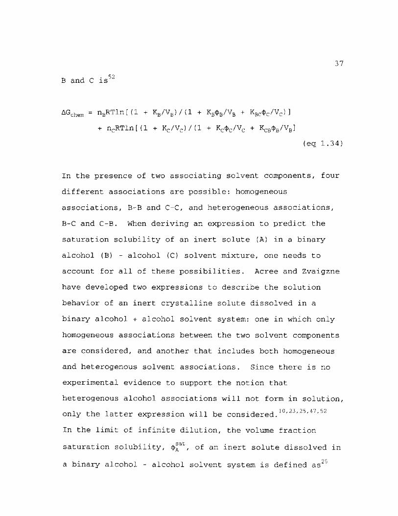
AGchem = nBRTln[(l + KB/VB)/(1 + KB$B/VB + KBCcf>c/Vc) ]

+ ncRTln [ (1 + Kc/Vc)/(1 + Kcct>c/Vc + KCBc()B/VB]

(eg 1.34)

In the presence of two associating solvent components, four

different associations are possible: homogeneous

associations, B-B and C-C, and heterogeneous associations,

B-C and C-B. When deriving an expression to predict the

saturation solubility of an inert solute (A) in a binary

alcohol (B) - alcohol (C) solvent mixture, one needs to

account for all of these possibilities. Acree and Zvaigzne

have developed two expressions to describe the solution

behavior of an inert crystalline solute dissolved in a

binary alcohol + alcohol solvent system: one in which only

homogeneous associations between the two solvent components

are considered, and another that includes both homogeneous

and heterogenous solvent associations. Since there is no

experimental evidence to support the notion that

heterogenous alcohol associations will not form in solution,

10 9 3 9 R 47 R 9

only the latter expression will be considered. • • • •

In the limit of infinite dilution, the volume fraction

saturation solubility, of an inert solute dissolved in a binary alcohol - alcohol solvent system is defined as 25

38

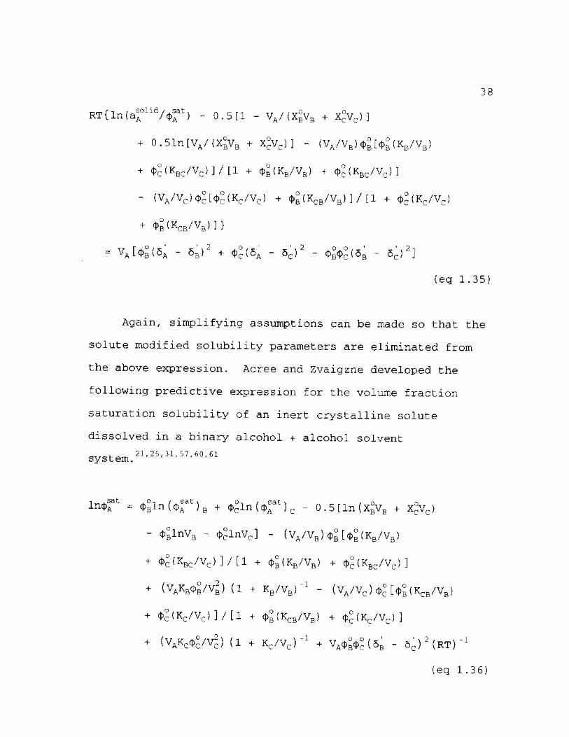
RT{ln(aAoli%A

at) - 0.5 [1 - VA/ (X°VB + X°VC) ]

+ 0.51n[VA/(X°VB + X ° V C ) ] - ( V A / V B ) ^ ° [ C } ) ° ( K B / V B )

+ C|)^ ( K B C / V C ) ] / [ 1 + (J)B ( K B / V B ) + (£>£ ( K B C / V C ) ]

- (VA/Vc)ct>°[c|>°(Kc/Vc) + 0 ° ( K C B / V B ) ] / [ 1 + 4 > C ( K C / V C )

+ 0 B ( K C B / V B ) ] }

= V A [ < ( 5 ; - 5 g ) 2 + - 5 , 1 ) 2 - <t>°<|>°(6B - S ^ ) 2 ]

(eg 1.35)

Again, simplifying assumptions can be made so that the

solute modified solubility parameters are eliminated from

the above expression. Acree and Zvaigzne developed the

following predictive expression for the volume fraction

saturation solubility of an inert crystalline solute

dissolved in a binary alcohol + alcohol solvent

system.21'25'31'57'60'61

lncJ)Aat = 0°ln (cj)A

at) B + cj>°ln ((t>Aat) c - 0 .5 [In (XBVB + X°VC)

" <f>BlnVB - ct>°lnVc] " (VA/VB)(j)B[cj)B(KB/VB)

+ <t>?(KBc/Vc)]/[l + <|>B(KB/Vb) + (Kbc/Vc) ]

+ (VAKBcp° /V 2 ) ( 1 + K G / V G ) - 1 - ( V A / V C ) C J ) ° [ C J ) ° ( K C B / V B )

+ < J ) ° ( K C / V C ) ] / [ 1 + 4>B ( K C B / V B ) + 0 ° ( K C / V C ) ]

+ (VAKC(J>°/V2) (1 + Kc/Vc)

1 + VAc{)°(t)°(5B - 5,1) 2 (RT)"1

(eg 1.36)

39

The homogeneous association complex constants are

denoted by KB and Kc for solvent B and C, respectively. KBC

and Kcb are the heterogeneous association constants for the

B-C and C-B associations, respectively. In several

previous studies Acree and coworkers discovered that a

single value of 5,000 cm3 mol 1 for all homogeneous and

heterogeneous association constants, regardless of the

alcohol, led to very accurate predictions of anthracene and

pyrene solubility behavior in binary alcohol + alcohol

27

solvent mixtures. Mobile Order theory predicted the

observed mole fraction solubility data to within an overall

absolute deviation of less than 3 %. Deviations did

decrease slightly when the authors used alcohol-specific

association constants calculated from binary liquid-vapor

equilibrium data for alkane + alcohol systems. The slight

0.3 % improvement in predictive accuracy did not warrant the

increased calculational complexity or time required to

parameterize the vapor-liquid equilibrium data in the Kc . . • 25,50

computation.

40

Chapter References

1. McHale, M. E. R.; Kauppila, A.-S. M.; Powell, J. R. ; Otero, P., Jr.; Jayasekera, M.; Acree, W. E., Jr. J. Soln. Chem. 1996 25, 295-302.

2. Acree, W. E., Jr.; Tucker, S. A.; Zvaigzne, A. I. Phys. Chem. Liq. 1990 21, 45-49.

3. Ruelle, P.; Buchmann, M.; Nam-Tran, H.; Kesselring, U. W. Int. J. Pharm. 1992 87, 47-57.

4. Huyskens, P. L.; Siegel, G. G. Bull. Soc. Chim. Belg. 1988 97, 821-824.

5. Ruelle, P.; Rey-Mermet, C.; Buchmann, M.; Nam-Tran, H.; Kesselring, U. W.; Huyskens, P.L. Pharm. Res. 1991 8, 840-850.

6. Ruelle, P.; Sarraf, E.; Van den Berge, L.; Seghers, K.; Buchmann, M.; Kesselring, U. W. Pharm. Acta Helv. 1993 68, 49-60.

7. Seigel, G. G.; Huyskens, P. L.; Vanderheyden G. Ber. Bunsenges. Phys. Chem. 1990 94, 549-553.

8. Huyskens, P. L. J. Mol. Struct. 1992 270, 197-203.

9. Nelis, K.; Van den Berge-Parmentier, L.; Huyskens, F. J. Mol. Liq. 1995 67, 157-174.

10. Huyskens, P. L.; Huyskens, D. P.; Siegel, G. G. J. Mol. Liq. 1995 64, 283-300.

11. Huyskens, P. L.; Seghers, K. J. Mol. Struct. 1994 322, 75-82 .

12. Huyskens, P. L. J. Mol. Struct. 1993 97, 141-147.

13. Ruelle, P.; Buchmann, M.; Kesselring, U. W. J. Pharm. Sci. 1994 83, 369-403.

14. McCargar, J. W.; Acree, W. E., Jr. J. Soln. Chem. 1988 17, 1081-1091.

15. Acree, W. E., Jr. Encyclopedia of Physical Science and Technology, Vol 11; Academic Press: Orlando FL, 1992, 1-22 .

16. Huyskens, P. L.; Vael-Pauwels, C.; Seghers, K. Bull. Soc. Chim. Belg. 1992 101, 449-462.

41

17. Huyskens, P. L.; Haulait-Pirson, M. C. J. Coat. Tech. 1985 57, 57-67.

18. Huyskens, P.; Kapuku, F.; Colemants-Vandevyvere, C. J. Mol. Struct. 1990 237, 207-220.

19. Acree, W. E., Jr.; McCargar, J. W. J. Mol. Liq. 1988 37, 251-261.

20. Acree, W. E., Jr.; Zvaigzne, A. I.; Tucker, S. A. Fluid Phase Equil. 1994 92, 1-17.

21. Zvaigzne, A. I.; Powell, J. R.; Acree, W. E., Jr.; Campbell, S. W. Phys. Chem Liq. 1996 121, 1-13.

22. Powell, J. R.; Acree, W. E., Jr.; Huyskens, P. L. submitted for publication in J. Soln. Chem.

23. McHale, M. E. R.; Pandey, S.; Acree, W. E., Jr. Phys. Chem. Liq., 1996 33, 93-112.

24. Acree, W. E., Jr.; Zvaigzne, A. I.; Tucker, S. A. Fluid Phase Equil. 1994 92, 233-253.

25. Powell, J. R.; Fletcher, K. A.; Coym, K. S.; Acree, W. E., Jr.; Varanasi, V. G.; Campbell, S. W. submitted for publication in J. Int. Thermophys.

26. Zvaigzne, A. I.; Teng, I.-L.; Martinez, E.; Trejo, J.; Acree, W. E., Jr. J. Chem. Eng. Data 1993 38, 389-392.

27. Acree, W. E., Jr.; Zvaigzne, A. I. Fluid Phase Equil. 1994 99, 167-183.

28. Powell, J. R.; McHale, M. E. R.; Kauppila, A.-S. M.; Otero, P.; Jayasekera, M.; Acree, W. E., Jr. J. Chem. Eng. Data 1992 40, 1270-1272.

29. Zvaigzne, A. I.; Acree, W. E., Jr. J. Chem. Eng. Data 1995 40, 917-919.

30. Zvaigzne, A. I.; McHale, M. E. R.; Powell, J. R.; Kauppila, A.-S. M.; Acree, W. E., Jr., J. Chem. Eng. Data 1995 40, 1273-1275.

31. Acree, W. E., Jr.; Tucker, S. A. Fluid Phase Equil. 1994 102, 17-29.

32. Acree, W. E., Jr.; Tucker, S. A. Int. J. Pharm. 1994 101, 199-207.

42

33. Powell, J. R.; McHale, M. E. R.; Kauppila, A.-S. M.; Acree, W. E., Jr.; Campbell, S. W. J. Sol. Chem. 1996 25, 1001-1017.

34. McHale, M. E. R.; Powell, J. R.; Kauppila, A.-S. M.; Acree, W. E., Jr.; Huyskens, P. L. J. Sol. Chem., in press.

35. Ruelle, P.; Buchmann, M.; Nam-Tran, H.; Kesselring, U. W. J. Comp. Aid. Design 1992, 431-448.

36. Ruelle, P.; Buchmann, M.; Nam-Tran, H.; Kesselring, U. W. Pharm. Res. 1992 9, 788-791.

37. Ruelle, P.; Sarraf, E.; Kesselring, U. W. Int. J. Pharm. 1994 104, 125-133.

38. Ruelle, P.; Sarraf, E.; Van den Berge, L.; Seghers, K.; Buchmann, M.; Kesselring, U. W. Pharm. Acta Helv. 1993 68, 49-60.

39. Ruelle, P.; Kesselring, U. W. J. Mol. Liq. 1995 67, 81-94.

40. Ruelle, P.; Kesselring, U. W. Phaim. Res. 1994 11, 201-205.

41. Ruelle, P.; Buchmann, M.; Nam-Tran, H; Kesselring, U. W. Environ. Sci. Techno1. 1993 27, 266-270.

42. Acree, W. E., Jr. Thermodynamic Properties of Nonelectrolyte Solutions; Academic Press: Orlando, Fl, 1984; Chapter 3.

43. Acree, W. E., Jr. Thermochim. Acta 1992 198, 71-79.

44. Acree, W. E., Jr. Thermodynamic Properties of Nonelectrolyte Solutions; Academic Press: Orlando, Fl, 1984; Chapter 10.

45. Acree, W. E., Jr. Thermodynamic Properties of Nonelectrolyte Solutions; Academic Press: Orlando, Fl, 1984; Chapter 2.

46. Ruelle, P.; Kesselring, U. W. J. Sol. Chem. 1996 25, 657-665.

47. Huyskens, P.; Van Beylen, M.; Verheyden, H. Pure and Appl. Chem. 1996 68, 1530-1540.

48. Huyskens, P. L. J. Mol. Struct. 1992 274, 223-246.

43

49. Huyskens, P. L. J. Am. Chem. Soc. 1977 99, 2578-2582.

50. Acree, W. E., Jr. Current Topics in Sol. Chem. 1994 1-30 .

51. Huyskens, P. L.; Haulait-Pirson, M. C. J. Mol. Liq. 1985 31, 135-151.

52. Huyskens, P. L.; Haulait-Pirson, M. C.; Siegel, G. G.; Kapuku, F. J. Phys. Chem. 1988 92, 6481-6847.

53. Burchfield, T. E.; Bertrand, G. L. J. Sol. Chem. 1975 4, 205-214.

54. Acree, W. E., Jr.; Bertrand, G. L. J. Phys. Chem. 1977 81, 1170-1173.

55. Acree, W. E., Jr.; Bertrand, G. L. J. Sol. Chem. 1983 12, 101-113.

56. Acree, W. E., Jr. Thermodynamic Properties of Nonelectrolyte Solutions; Academic Press: Orlando, Fl, 1984; Chapter 5.

57. Acree, W. E., Jr.; Zvaigzne, A. I. Fluid Phase Equil. 1994 99, 167-183.

58. Acree, W. E., Jr.; Rytting, J. H. J. Pharm. Sci. 1983 72, 292-296.

59. Pandey, S.; Powell, J. R.; McHale, M. E. R.; Kauppila, A.-S. M.; Acree, W. E., Jr. Fluid Phase Equil. 1996 123, 29-38.

60. McHale, M. E. R.; Zvaigzne, A. I.; Powell, J. R.; Kauppila, A.-S. M.; Acree, W. E., Jr.; Campbell, S. W. Phys. Chem. Liq 1996 32, 67-85.

61. Powell, J. R.; McHale, M. E. R.; Kauppila, A.-S. M.; Acree, W. E., Jr.; Campbell, S. W. J. Soln. Chem. 1996 25, 1001-1017.

CHAPTER II

EXPERIMENTAL PROCEDURES AND RESULTS

Materials

Benzil (98 %) , thianthrene (99+ %) , trans-stilbene

(96 %) , and thioxanthen-9-one (98 %) , diphenyl sulfone

(97 %) , and dibenzothiophene sulfone (97 %) were purchased

from Aldrich and recrystalized several times from anhydrous

methanol. n-Hexane (Aldrich, 99 %) , n-heptane (Sigma-

Aldrich, 99+ %, HPLC grade), n-octane (Aldrich, 99+ %,

anhydrous), cyclohexane (Aldrich, 99.9+ %, HPLC grade),

methylcyclohexane (Aldrich, 99+ %, anhydrous), cyclooctane

(Aldrich, 99+ %), 2,2,4-trimethylpentane (Aldrich, 99.7+ %,

HPLC grade), terfc-butylcyclohexane (Aldrich, 99+ %), benzene

(Aldrich, 99.9+ %, HPLC grade), toluene (Aldrich, 99.8 %,

HPLC grade), o-xylene (Aldrich, HPLC grade), .m-xylene

(Aldrich, 99+ %), p-xylene (Aldrich, HPLC grade), dibutyl

ether (Aldrich, 99 %), methyl tert-butyl ether (Arco,

99.9+ %), tetrahydrofuran (Sigma-Aldrich, 99.9+ %, HPLC

grade), 1,4-dioxane (Aldrich, 99.8+ %), 1-chlorobutane

(Aldrich, 99.9+ %), 1,2-dichloroethane (Aldrich, 99+ %,

anhydrous), ethyl acetate (Aldrich, 99.9 %), butyl acetate

(Aldrich, 99.8+ %), methanol (Aldrich, 99.9+ %), ethanol

45

(Aaper Alcohol and Chemical Company, absolute), 1-propanol

(Aldrich, 99+ %, anhydrous), 2-propanol (Aldrich, 99+ %,

anhydrous), 1-butanol (Aldrich 99.8+ %, HPLC grade),

2-butanol (Aldrich, 99+ %, anhydrous), 2-methyl-1-propanol

(Aldrich, 99+ %, anhydrous), 1-pentanol (Aldrich, 99+ %), 2-

pentanol (Acros, 99+ %), 3-methyl-1-butanol (Aldrich, 99+ %,

anhydrous), 2-methyl-2-butanol (Acros, 99+ %) , 1-hexanol

(Alfa Aesar, 99+ %), 4-methyl-l-pentanol (Acros, 99+ %) ,

2-methyl-2-pentanol (Aldrich, 99 %), 1-heptanol (Alfa Aesar,

99+ %), 1-octanol (Aldrich, 99+ %), 2-ethyl-1-hexanol

(Aldrich, 99+ %), and cyclopentanol (Aldrich, 99 %) were

stored over molecular sieves before use to remove trace

amounts of water. Karl Fischer titration gave a water

content of mass/mass % of <0.01 % or better for all alcohol

solvents. Gas chromatographic analysis showed solvent

purities to be 99.7 mole percent or better.

Experimental Procedures and Results:

Pure Solvent Studies

For each study, excess solute and solvent were placed

in 8 oz. amber glass bottles. The bottle cap was teflon

lined, sealed with parafilm and vinyl electrical tape, and

then secured with a rubber band. These precautionary

measures were taken in order to prevent the contamination of

the samples by water and also to reduce the possibility of

46

evaporation of the more volatile solvents.

The sample bottles were allowed to approach equilibrium

from supersaturation by pre-equilibrating the solutions at a

higher temperature. The bottles were then placed in a

constant temperature water bath (25.0 ± 0.1 °C) for at least

three days, but often longer. Attainment of equilibrium was

verified by random repetitive measurements after several

additional days in the constant temperature water bath and

also by the pre-equilibration step. To determine the amount

of sample needed, aliquots of saturated solution were

syringed and transferred through a course filter into a

tared volumetric flask, and then diluted quantitatively with

methanol for spectrophotmetric analysis at the appropriate

wavelength using a Bausch and Lomb Spectronic 2000. All

volumetric glassware was of grade A tolerance.

For each solute, concentrations of the dilute solutions

were determined from a Beer Lambert absorbance versus

concentration working curve which was derived from the

absorbance of at least nine standard solutions of known

concentration. Every attempt was made to ensure the

absorbance measurements fell within the linear region of the

Beer-Lambert working curve, however, systems were diluted to

a sufficient level when their measured absorbances were not

within this region. Spectrochemical data for all solutes

studied is listed in Table I. The molar absorptivities of

each solute were determined from the standard solutions.

47

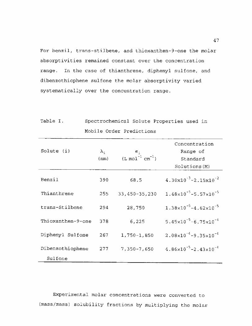
For benzil, trans-stilbene, and thioxanthen-9-one the molar

absorptivities remained constant over the concentration

range. In the case of thianthrene, diphenyl sulfone, and

dibenzothiophene sulfone the molar absorptivity varied

systematically over the concentration range.

Table I. Spectrochemical Solute Properties used in

Mobile Order Predictions

Solute (i]

(nm) 1

(L mol-1 cm"1)

Concentration

Range of

Standard

Solutions(M)

Benzil 390 68.5 4 . 3 0x10 3-2 .15x10 2

Thianthrene 255 33,450-35,230 1. 48xl0~5-5 . 57xl0~5

trans-Stilbene 294

Thioxanthen-9-one 378

Diphenyl Sulfone 267

Dibenzothiophene 277

Sulfone

28,750

6,225

1,750-1,850

7,350-7,650

1.38X10"5-4.62X10~5

5.45X10"5-6.75X10-4

2.08X10~4-9.35X10~4

4.86X10"5-2 .43x10 ~4

Experimental molar concentrations were converted to

(mass/mass) solubility fractions by multiplying the molar

48

mass of the solute by the volume(s) of the volumetric flasks

used and any required dilutions. This value was then

divided by the mass of the saturated solute analyzed. Mole

fraction solubilities were computed from (mass/mass)

solubility fractions using the molar masses of the solute

and solvent, and are listed in Tables II - VII. Numerical

values represent the average of between four and eight

independent determinations in each of the solutes. For

thianthrene, fcrans-stilbene, thioxanthen-9-one, diphenyl

sulfone, and dibenzothiophene sulfone measurements were

reproducible to ± 2 %, and for benzil the measured

solubilities reported were reproducible from ±1.5 % for

solvents having the lower mole fraction solubilities to

± 2.5 % for solvents having higher benzil solubilities.

Benzil Study in Pure Solvents

Benzil was dissolved in twenty-three pure organic

nonelectrolyte solvents, each possessing free electron pairs

capable of participating in hydrogen bonding or dipole-

dipole interactions. Experimental values for the mole

fraction saturation solubility of benzil in solvents

incapable of self association were obtained from the

1-4

literature. The solvents studied were tetrahydrofuran,

1,4-dioxane, 1-chlorobutane, 1,2-dichloroethane, ethyl

acetate, butyl acetate, methanol, ethanol, 1-propanol,

49

2-propanol, 1-butanol, 2-butanol, 2-methyl-1-propanol,

1-pentanol, 2-pentanol, 3-methyl-l-butanol, 2-methyl-2-

butanol, 1-hexanol, 4-methyl-2-pentanol, 1-heptanol,

1-octanol, 2-ethyl-1-hexanol, and cyclopentanol. Solvent

purities are noted at the beginning of this chapter. The

concentration of benzil in each dilute solution was

determined from standard solutions of known concentrations

ranging from 4.30x10 3 molar to 2.15x10 2 molar. The

calculated molar absorptivity of e » 65.8 L mol 1 cm 1 was

constant over the above concentration range. Experimental

mole fraction solubilities for benzil are listed in

Table II.5

Thianthrene Study in Pure Solvents

Thianthrene was studied in twenty-one neat organic

nonelectrolyte solvents. Previous studies By Acree, Tucker,

and Zvaigzne reported thianthrene solubilities in neat

alkane solvents , therefore the bulk of this work focused on

self associating solvents and other alkanes not previously

studied: tert-butylcyclohexane, dibutyl ether, methyl tert-

butyl ether, methanol, ethanol, 1-propanol, 2-propanol,

1-butanol, 2-butanol, 2-methyl-1-propanol, 1-pentanol,

2-pentanol, 3-methyl-l-butanol, 2-methyl-2-butanol,

1-hexanol, 4-methyl-l-pentanol, 4-mehtyl-2-pentanol,

1-hepanol, 1-octanol, 2-ethyl-l-hexanol, and cyclopentanol.

50

Experimental thianthrene concentration in the dilute

solutions were determined from standard solutions ranging in

-5 -5

concentration from 1.48x10 to 5.57x10 molar. The molar

absorptivity of thianthrene varied from 35,230 to 33,450 L

mol 1 cm 1 throughout the concentration range. Experimentally

determined saturation mole fraction solubilities for

thianthrene are listed in Table III.7

trans-Stilbene Study in Pure Solvents

The solubility of trans-stilbene was investigated in

twenty-eight neat organic self-associating and

nonassociating nonelectrolyte solvents containing ether-,

hydroxy-, methyl-, and t-butyl functional groups. The

specific solvents studied were: n-hexane, n-heptane,

n-octane, cyclohexane, methylcyclohexane, cyclooctane,

2,2,4-trimethylpentane, tert-butylcyclohexane, dibuyl ether,

methyl tert-butyl ether, methanol, ethanol, 1-propanol,

2-propanol, 1-butanol, 2-butanol, 2-methyl-l-propanol,

1-pentanol, 2-pentanol, 3-methyl-l-butanol, 2-methyl-2-

butanol, 1-hexanol, 2-methyl-l-pentanol, 4-methyl-2-

pentanol, 1-heptanol, 1-octanol, 2-ethyl-l-hexanol, and

cyclopentanol, with their purities reported at the beginning

of this chapter. The concentration of trans-stilbene in

each solvent system was determined from standard solutions

of known concentration ranging from 1.38xl0~5 to 4.62xl0~5

51

molar, with its molar absorptivity remaining constant at

e « 28,750 L mol-1 cm'1. Experimental saturation mole

fraction solubilities for fcrans-stilbene are listed in

Table IV.8

Thioxanthen-9-one Study in Pure Solvents

Thioxanthen-9-one was investigated in thirty-five

organic self-associating and non self-associating

nonelectrolyte solvents: n-hexane, n-heptane,

n-octane, cyclohexane, methylcyclohexane, cyclooctane,

2,2,4-trimethylpentane, tert-butylcyclohexane, benzene,

toluene, o-xylene, in-xylene, p-xylene, dibutyl ether, methyl

tert-butyl ether, ethyl acetate, butyl acetate, methanol,

ethanol, 1-propanol, 2-propanol, 1-butanol, 2-butanol,

2-methyl-1-propanol, 1-pentanol, 2-pentanol, 3-methyl-l-

butanol, 2-methyl-2-butanol, 1-hexanol, 2-methyl-1-pentanol,

4-methyl-2-pentanol, 1-heptanol, 1-octanol, 2-ethyl-l-

hexanol, and cyclopentanol. The concentration of

thioxanthen-9-one in the pure solvent systems was determined

from standard solutions which ranged in concentration from

- 5 - 4 • 5.45x10 to 6.75x10 molar. The molar absorptivity of

- 1 - 1

thioxanthen-9-one was determined to be 6,225 L mol cm .

Experimental mole fraction solubilities for thioxanthen-9-9

one are listed m Table V.

52

Diphenyl Sulfone Study

Diphenyl sulfone was studied in twenty-four neat

organic nonelectrolyte alkane and self-associating solvents

containing alkane or alcohol substituents. The solvents

used were n-hexane, n-heptane, n-octane, cyclohexane,

methylcyclohexane, cyclooctane, 2,2,4-trimethylpentane,

tert-butylcyclohexane, methanol, ethanol, 1-propanol,

2-propanol, 1-butanol, 2-butanol, 2-methyl-1-propanol,

1-pentanol, 2-pentanol, 3-methyl-l-butanol, 1-hexanol,

2-methyl-l-pentanol, 4-methyl-2-pentanol, 1-heptanol,

1-octanol, and 2-ethyl-l-hexanol. The molar absorptivity of

diphenyl sulfone varied from 1,750 L mol 1 cm 1 to

1,850 L mol 1 cm"1 over the concentration range of 2.08x10 4

molar to 9.35xl0~4 molar. Experimental mole fraction

solubilities of diphenyl sulfone are listed in Table VI.

Dibenzothiophene Sulfone Study

Dibenzothiophene sulfone was dissolved in twenty-six

different neat solvent systems ranging from straight alkane

chains to branched self-associating alcohol solvents. The

solvents studied were .n-hexane, n-heptane, n-octane,

cyclohexane, methylcyclohexane, cyclooctane,

2,2,4-trimethylpentane, tert-butylcyclohexane, methanol,

ethanol, 1-propanol, 2-propanol, 1-butanol, 2-butanol,

53

2-methyl-1-propanol, 1-pentanol, 2-pentanol, 3-methyl-1-

butanol, 2-methyl-2-butanol, 1-hexanol, 2-methyl-1-pentanol,

4-methyl-2-pentanol, 1-heptanol, 1-octanol, 2-ethyl-l-

hexanol, and cyclopentanol. Solvent purities were noted at

the beginning of this chapter. The concentration of

dibenzothiophene sulfone in each dilute solution was

determined from standard solutions of known concentrations

-5 -4

ranging from 4.86x10 molar to 2.43x10 molar with its

calculated molar absorptivity varying systematically from

7,350 L mol 1 cm 1 to 7,650 L mol 1 cm 1 throughout this range.

Experimental mole fraction solubilities are listed in

Table VII.

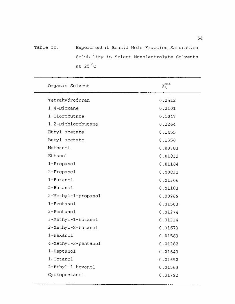
54

Table II. Experimental Benzil Mole Fraction Saturation

Solubility in Select Nonelectrolyte Solvents

at 25 °C

Organic Solvent X sat

Tetrahydrofuran

1,4-Dioxane

1-Clorobutane

1,2-Dichlorobutane

Ethyl acetate

Butyl acetate

Methanol

Ethanol

1-Propanol

2-Propanol

1-Butanol

2-Butanol

2-Methyl-1-propanol

1-Pentanol

2-Pentanol

3-Methyl-1-butanol

2-Methyl-2-butanol

1-Hexanol

4-Methyl-2-pentanol

1-Heptanol

1-Octanol

2-Ethyl-1-hexanol

Cyclopentanol

0 .2512

0.2101

0.1047

0.2264

0.1455

0.1350

0.00783

0.01031

0.01184

0.00831

0.01306

0.01103

0.00969

0.01503

0.01274

0.01214

0.01673

0.01563

0.01282

0.01643

0.01692

0.01563

0.01792

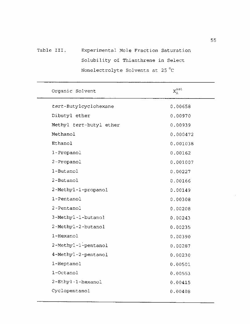
Table III.

55

Experimental Mole Fraction Saturation

Solubility of Thianthrene in Select

Nonelectrolyte Solvents at 25 °C

Organic Solvent X sat

tert-Butyleye1ohexane 0 .00658

Dibutyl ether 0 .00970

Methyl tert-butyl ether 0 .00939

Methanol 0 .000472

Ethanol 0 .001038

1-Propanol 0 .00162

2-Propanol 0 .001007

1-Butanol 0 .00227

2-Butanol 0 .00166

2-Methyl-1-propanol 0 .00149

1-Pentanol 0 .00308

2-Pentanol 0 .00208

3-Methyl-1-butanol 0 .00243

2-Methyl-2-butanol 0 .00235

1-Hexanol 0 .00390

2-Methyl-1-pentanol 0 .00287

4-Methyl-2-pentanol 0 .00230

1-Heptanol 0 .00501

1-Octanol 0 .00553

2-Ethyl-l-hexanol 0 .00415

Cyclopentanol 0 .00408

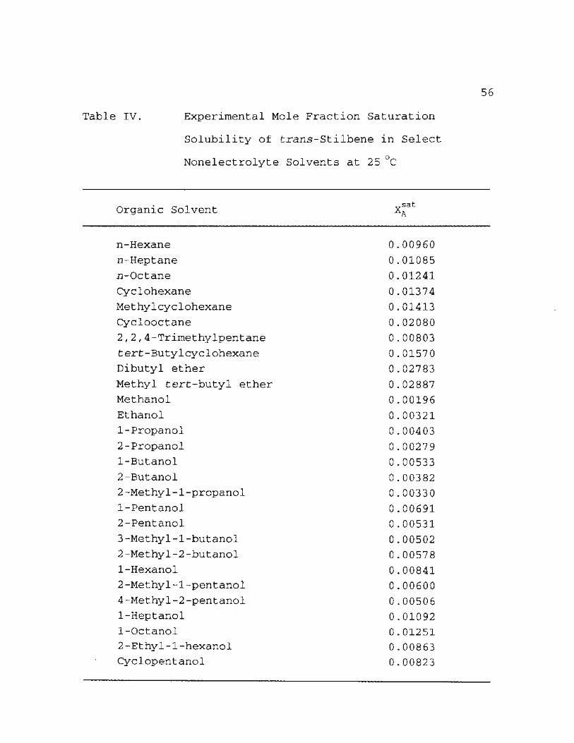
Table IV.

56

Experimental Mole Fraction Saturation

Solubility of fcrans-Stilbene in Select

Nonelectrolyte Solvents at 25 °C

Organic Solvent X sat

n-Hexane 0 .00960 n-Heptane 0 .01085 n-Octane 0 .01241 Cyclohexane 0 .01374 Methylcyclohexane 0 .01413 Cyclooctane 0 .02080 2,2,4-Trimethylpentane 0 .00803 tert-Butylcyclohexane 0 .01570 Dibutyl ether 0 .02783 Methyl tert-butyl ether 0 .02887 Methanol 0 .00196 Ethanol 0 .00321 1-Propanol 0 .00403 2-Propanol 0 .00279 1-Butanol 0 .00533 2-Butanol 0 .00382 2-Methyl-1-propanol 0 .00330 1-Pentanol 0 .00691 2-Pentanol 0 .00531 3-Methyl-1-butanol 0 .00502 2-Methyl-2-butanol 0 .00578 1-Hexanol 0 .00841 2-Methyl-1-pentanol 0 .00600 4-Methyl-2-pentanol 0 .00506 1-Heptanol 0 .01092 1-Octanol 0 .01251 2-Ethyl-1-hexanol 0 .00863 Cyclopentanol 0 .00823

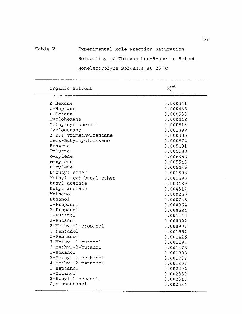
Table V.

57

Experimental Mole Fraction Saturation

Solubility of Thioxanthen-9-one in Select

Nonelectrolyte Solvents at 25 °C

Organic Solvent X sat

ii-Hexane 0 .000341 n-Heptane 0 .000436 n-Octane 0 .000533 Cyclohexane 0 .000448 Methylcyclohexane 0 .000513 Cyclooctane 0 .001399 2,2,4-Trimethylpentane 0 .000305 tert-Butylcyclohexane 0 .000674 Benzene 0 .005181 Toluene 0 .005188 o-xylene 0 .006358 m-xylene 0 .005543 p-xylene 0 .005436 Dibutyl ether 0 .001508 Methyl fcerfc-butyl ether 0 .001598 Ethyl acetate 0 .003489 Butyl acetate 0. .004317 Methanol 0 .000260 Ethanol 0 .000738 1-Propanol 0 .000864 2-Propanol 0 .000684 1-Butanol 0 .001140 2-Butanol 0 .000999 2-Methyl-1-propanol 0 .000907 1-Pentanol 0 .001554 2-Pentanol 0 .001426 3-Methyl-1-butanol 0 .001193 2-Methyl-2-butanol 0 .001478 1-Hexanol 0 .001908 2-Methyl-1-pentanol 0 .001732 4-Methyl-2-pentanol 0 .001397 1-Heptanol 0 .002294 1-Octanol 0 .002839 2-Ethyl-1-hexanol 0 .002313 Cyclopentanol 0 .002324

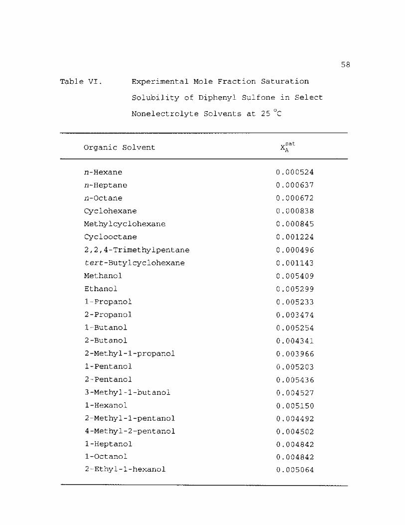
Table VI.

58

Experimental Mole Fraction Saturation

Solubility of Diphenyl Sulfone in Select

Nonelectrolyte Solvents at 25 °C

Organic Solvent X sat

n-Hexane 0 .000524

n-Heptane 0 .000637

n-Octane 0 .000672

Cyclohexane 0 .000838

Methylcyclohexane 0 .000845

Cyclooctane 0 .001224

2,2,4-Trimethylpentane 0 .000496

fcerfc-Butylcyclohexane 0 .001143

Methanol 0 .005409

Ethanol 0 .005299

1-Propanol 0 .005233

2-Propanol 0 . 003474

1-Butanol 0 .005254

2-Butanol 0 .004341

2-Methyl-1-propanol 0 .003966

1-Pentanol 0 .005203

2-Pentanol 0 .005436

3-Methyl-1-butanol 0 .004527

1-Hexanol 0 .005150

2-Methyl-1-pentanol 0 .004492

4-Methyl-2-pentanol 0 .004502

1-Heptanol 0 .004842

1-Octanol 0 .004842

2-Ethyl-1-hexanol 0 .005064

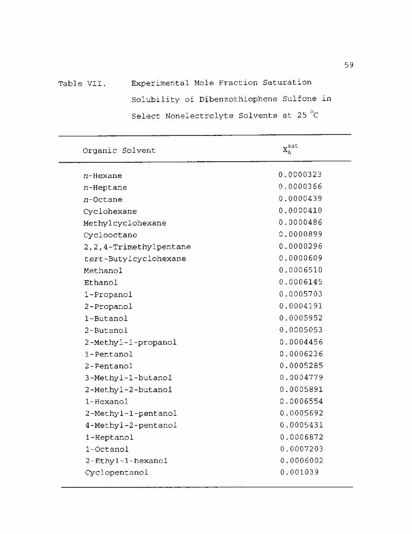
Table VII.

59

Experimental Mole Fraction Saturation

Solubility of Dibenzothiophene Sulfone in

Select Nonelectrolyte Solvents at 25 °C

Organic Solvent X sat

n-Hexane 0 .0000323

n-Heptane 0 .0000366

n-Octane 0 .0000439

Cyclohexane 0 .0000410

Methylcyclohexane 0 .0000486

Cyclooctane 0 .0000899

2,2,4-Trimethylpentane 0 .0000296

tert-Butylcyclohexane 0 .0000609

Methanol 0 .0006510

Ethanol 0 .0006145

1-Propanol 0 .0005703

2-Propanol 0 .0004191

1-Butanol 0 .0005952

2-Butanol 0 .0005053

2-Methyl-1-propanol 0 .0004456

1-Pentanol 0 .0006236

2-Pentanol 0 .0005285

3-Methyl-1-butanol 0 .0004779

2-Methyl-2-butanol 0 .0005891

1-Hexanol 0 .0006554

2-Methyl-l-pentanol 0 .0005692

4-Methyl-2-pentanol 0 .0005431

1-Heptanol 0 .0006872

1-Octanol 0 .0007203

2-Ethyl-1-hexanol 0 .0006002

Cyclopentanol 0 .001039

60

Experimental Procedure: Binary Solvent Studies

Benzil was dissolved in eight binary (alcohol +

1-octanol) solvent systems, where the "alcohol" component

consisted of 1-propanol, 2-propanol, 1-butanol, 2-butanol,

2-methyl-1-propanol, 1-pentanol, 3-methyl-1-butanol, or

4-methyl-2-pentanol. Solvent purities were given in an

earlier section of this chapter. Binary solvent mixtures

were prepared by mass fractions so the compositions of each

system could be calculated to 0.0001 mole fraction.

The experimental procedures used to determine the mole

fraction solubility of benzil in binary solvent mixtures

mimics the procedures employed for the pure solvent systems.

Excess solute and solvent were placed in 8 oz. amber glass

bottles. The bottle cap was teflon lined, sealed with

parafilm and vinyl electrical tape, and then secured with a

rubber band. Just as with the pure solvent studies, these

precautionary measures were taken in order to prevent the

contamination of the samples.

The systems were allowed to equilibrate in a high

temperature water bath, and then placed in a constant

temperature water bath at 25 °C ± 0.05 °C for at least three

days to ensure the systems had in fact reached equilibrium.

Attainment of equilibrium was verified by random repetitive

measurements after several more days in the constant

temperature water bath and also by the high temperature

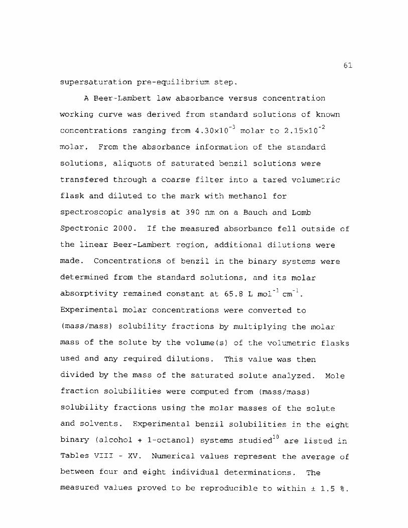
61

supersaturation pre-eguilibrium step.

A Beer-Lambert law absorbance versus concentration

working curve was derived from standard solutions of known

concentrations ranging from 4.3 0xl0~3 molar to 2.15xl0~2

molar. From the absorbance information of the standard

solutions, aliguots of saturated benzil solutions were

transfered through a coarse filter into a tared volumetric

flask and diluted to the mark with methanol for

spectroscopic analysis at 390 nm on a Bauch and Lornb

Spectronic 2000. If the measured absorbance fell outside of

the linear Beer-Lambert region, additional dilutions were

made. Concentrations of benzil in the binary systems were

determined from the standard solutions, and its molar

absorptivity remained constant at 65.8 L mol-1 cm"1.

Experimental molar concentrations were converted to

(mass/mass) solubility fractions by multiplying the molar

mass of the solute by the volume(s) of the volumetric flasks

used and any required dilutions. This value was then

divided by the mass of the saturated solute analyzed. Mole

fraction solubilities were computed from (mass/mass)

solubility fractions using the molar masses of the solute

and solvents. Experimental benzil solubilities in the eight

binary (alcohol + 1-octanol) systems studied10 are listed in

Tables VIII - XV. Numerical values represent the average of

between four and eight individual determinations. The

measured values proved to be reproducible to within ± 1.5 %.

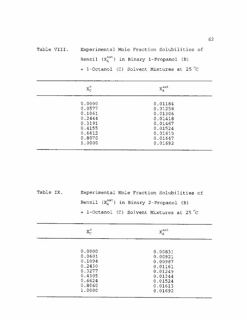
62

Table VIII. Experimental Mole Fraction Solubilities of

Benzil (X^at) in Binary 1-Propanol (B)

+ 1-Octanol (C) Solvent Mixtures at 25 °C

o u

XI sat A

0.0000 0.01184 0.0577 0.01258 0.1061 0.01306 0.2444 0.01418 0.3191 0.01467 0.4155 0.01524 0.6612 0.01615 0.8070 0.01647 1.0000 0.01692

Table IX. Experimental Mole Fraction Solubilities of

Benzil (X^at) in Binary 2-Propanol (B)

+ 1-Octanol (C) Solvent Mixtures at 25 °C

Xc sat XA

0.0000 0.00831 0.0601 0.00921 0.1094 0.00987 0.2430 0.01161 0.3277 0.01249 0.4305 0.01344 0.6624 0.01524 0.8060 0.01613 1.0000 0.01692

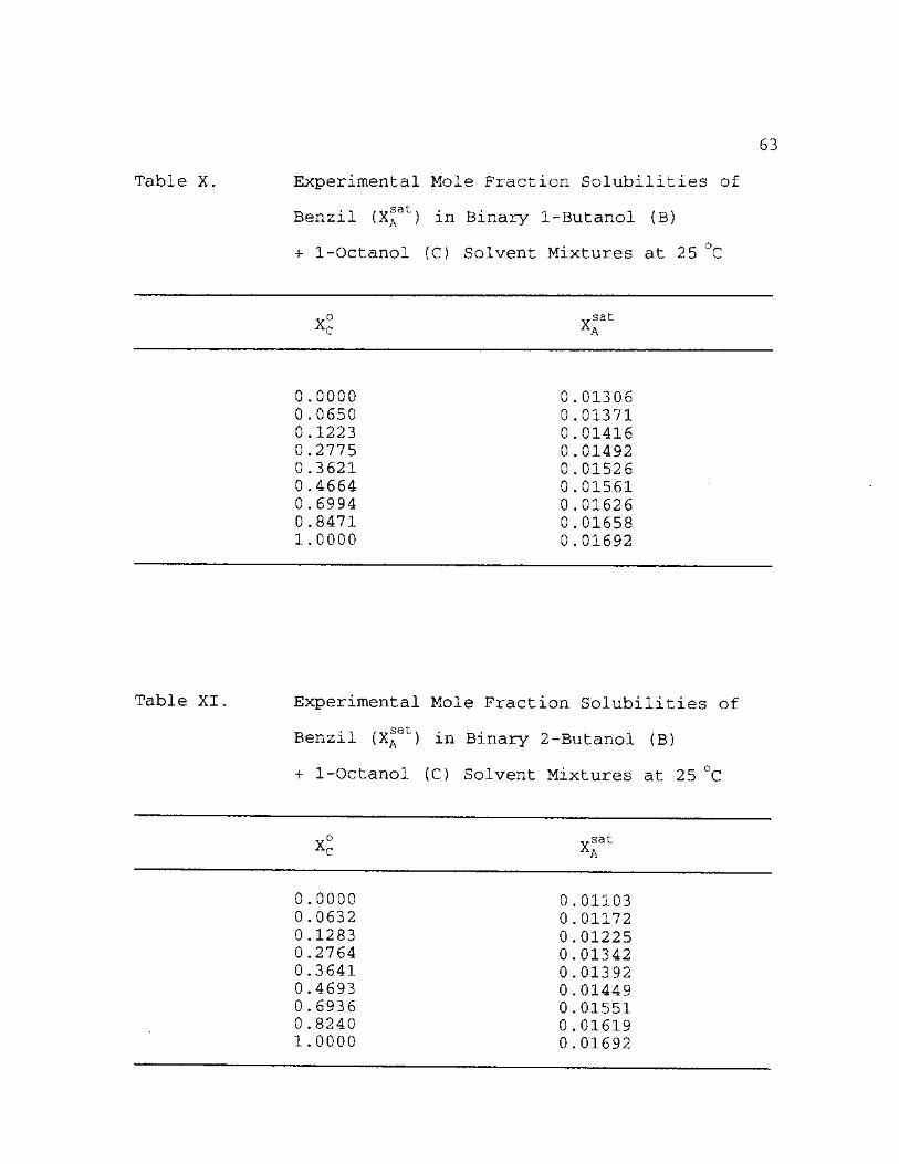
Table X.

63

Experimental Mole Fraction Solubilities of

Benzil (X^at) in Binary 1-Butanol (B)

+ 1-Octanol (C) Solvent Mixtures at 25 °C

Xc sat aA

0.0000 0.01306 0 .0650 0 .01371 0.1223 0.01416 0.2775 0.01492 0.3621 0.01526 0.4664 0.01561 0.6994 0.01626 0.8471 0.01658 1.0000 0.01692

Table XI. Experimental Mole Fraction Solubilities of

Benzil (X^at) in Binary 2-Butanol (B)

+ 1-Octanol (C) Solvent Mixtures at 25 °C

X

o o

vsat

0.0000 0.01103 0.0632 0.01172 0.1283 0.01225 0.2764 0.01342 0.3641 0.01392 0.4693 0.01449 0.6936 0.01551 0.8240 0.01619 1.0000 0.01692

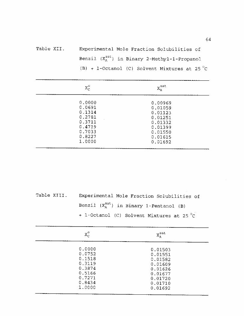
Table XII.

64

Experimental Mole Fraction Solubilities of

Benzil (X^at) in Binary 2-Methyl-l-Propanol

(B) + 1-Octanol (C) Solvent Mixtures at 25 °C

xc° sat

0.0000 0.00969 0.0691 0.01059 0.1314 0.01123 0.2781 0.01251 0.3711 0.01332 0.4719 0.01399 0.7033 0.01550 0.8227 0.01615 1.0000 0.01692

Table XIII. Experimental Mole Fraction Solubilities of

Benzil (X®at) in Binary 1-Pentanol (B)

+ 1-Octanol (C) Solvent Mixtures at 25 °C

X° sat A A

0.0000 0.01503 0.0752 0.01551 0.1518 0.01582 0.3119 0.01609 0.3874 0.01626 0.5166 0 .01677 0 .7271 0.01720 0.8434 0.01710 1.0000 0.01692

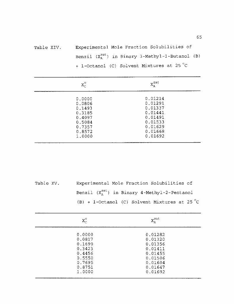
Table XIV.

65

Experimental Mole Fraction Solubilities of

Benzil (X^at) in Binary 3-Methyl-1-Butanol (B)

+ 1-Octanol (C) Solvent Mixtures at 25 °C

X

o o

Sat

A

0.0000 0.01214 0.0806 0.01291 0.1493 0.01337 0.3185 0.01441 0.4097 0.01491 0.5084 0.01533 0.7357 0.01629 0.8572 0.01668 1.0000 0.01692

Table XV. Experimental Mole Fraction Solubilities of

Benzil (X^at) in Binary 4-Methyl-2-Pentanol

(B) + 1-Octanol (C) Solvent Mixtures at 25 °C

o u

X sat

XA

0.0000 0.01282 0.0817 0.01320 0.1690 0.01356 0.3423 0.01411 0.4456 0.01455 0.5550 0.01506 0.7695 0.01604 0.8751 0.01647 1.0000 0.01692

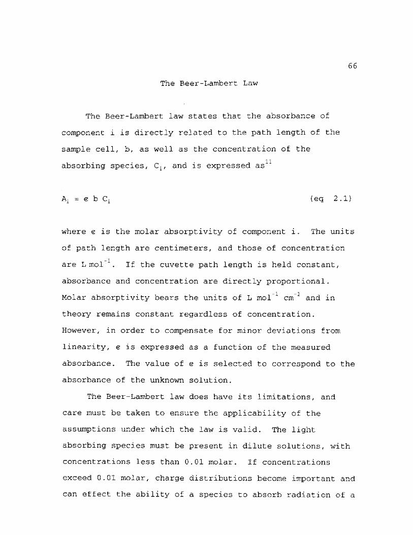
66

The Beer-Lambert Law

The Beer-Lambert law states that the absorbance of

component i is directly related to the path length of the

sample cell, b, as well as the concentration of the

11 absorbing species, Ci, and is expressed as

Ai = e b Ci (eq 2 .1)

where e is the molar absorptivity of component i. The units

of path length are centimeters, and those of concentration

are L mol 1. If the cuvette path length is held constant,

absorbance and concentration are directly proportional.

- 1 - 1

Molar absorptivity bears the units of L mol cm and in

theory remains constant regardless of concentration.

However, in order to compensate for minor deviations from

linearity, e is expressed as a function of the measured

absorbance. The value of e is selected to correspond to the

absorbance of the unknown solution.

The Beer-Lambert law does have its limitations, and

care must be taken to ensure the applicability of the

assumptions under which the law is valid. The light

absorbing species must be present in dilute solutions, with

concentrations less than 0.01 molar. If concentrations

exceed 0.01 molar, charge distributions become important and

can effect the ability of a species to absorb radiation of a

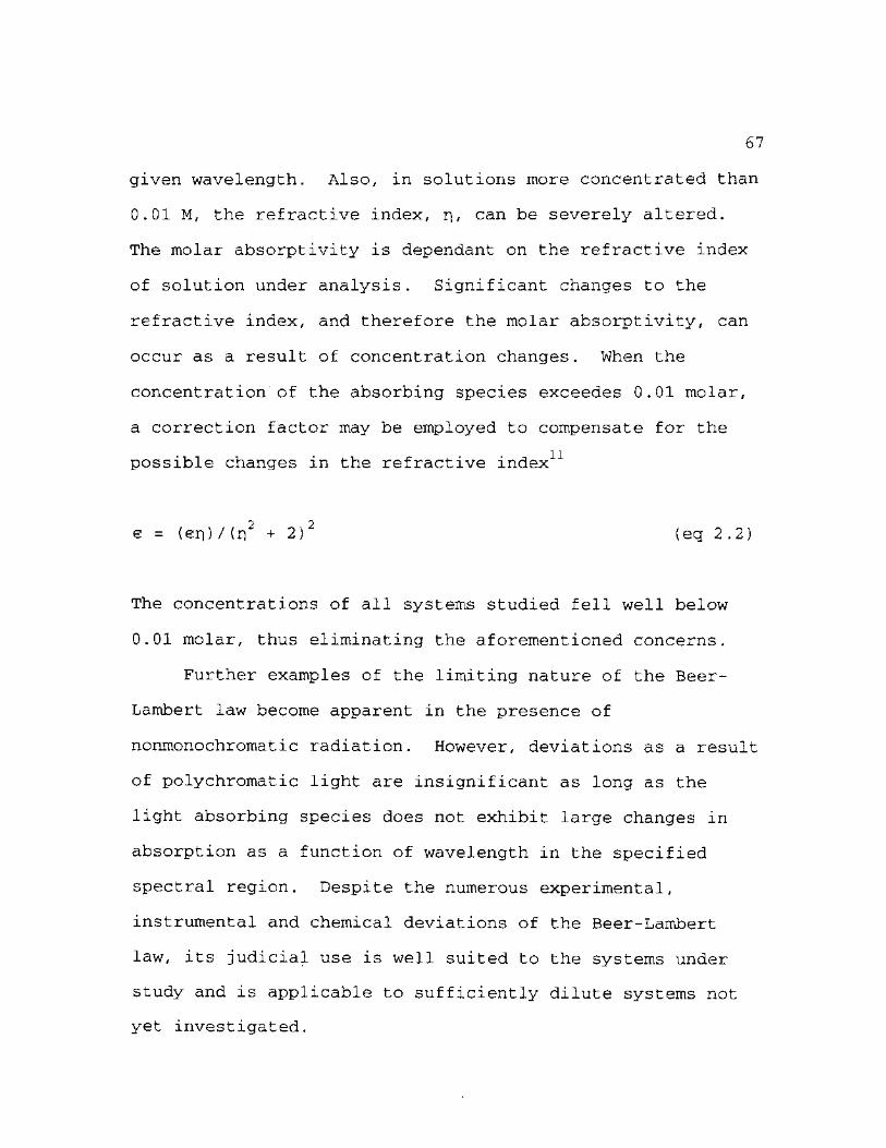
67

given wavelength. Also, in solutions more concentrated than

0.01 M, the refractive index, n, can be severely altered.

The molar absorptivity is dependant on the refractive index

of solution under analysis. Significant changes to the

refractive index, and therefore the molar absorptivity, can

occur as a result of concentration changes. When the

concentration of the absorbing species exceedes 0.01 molar,

a correction factor may be employed to compensate for the

possible changes in the refractive index11

e = ( e r i ) / ( r | 2 + 2 ) 2 (eg 2 .2 !

The concentrations of all systems studied fell well below

0.01 molar, thus eliminating the aforementioned concerns.

Further examples of the limiting nature of the Beer-

Lambert law become apparent in the presence of

nonmonochromatic radiation. However, deviations as a result

of polychromatic light are insignificant as long as the

light absorbing species does not exhibit large changes in

absorption as a function of wavelength in the specified

spectral region. Despite the numerous experimental,

instrumental and chemical deviations of the Beer-Lambert

law, its judicial use is well suited to the systems under

study and is applicable to sufficiently dilute systems not

yet investigated.

68

Chapter References

1. Acree, W. E., Jr.; Rytting, J. H. J. Pharm. Sci. 1982 71, 201-205.

2. Acree, W. E., Jr.; Bertrand, G. L. J. Sol. Chem. 1983 12, 101-113.

3. McHale, M. E. R.; Kauppila, A.-S. M.; Powell, J. R.; Otero, P., Jr,; Jayasekera, M.; Acree, W. E., Jr. J. Sol. Chem. 1996 25, 295-302.

4. McHale, M. E. R.; Kauppila, A.-S. M.; Powell, J. R.; Acree, W. E., Jr. Phys. Chem. Liq. 1996 31, 175-182.

5. Fletcher, K. A.; Pandey, S.; McHale, M. E. R.; Acree, W. E., Jr. Phys. Chem. Liq. 1996 33, 181-190.

6. Acree, W. E., Jr.; Tucker, S. A.; Zvaigzne, A. I. Phys. Chem. Liq. 1990 21, 45-49.

7. Fletcher, K. A.; McHale, M. E. R.; Powell, J. R.; Coym, K. S.; Acree, W. E., Jr. Phys. Chem. Liq., in press.

8. Fletcher, K. A.; McHale, M. E. R.; Coym, K. S.; Acree, W. E., Jr. Can. J. Chem., in press.

9. Fletcher, K. A.; Coym, K. S.; Roy, L. E.; Hernandez, C. E.; McHale, M. E. R.; Acree, W. E., Jr. Phys. Chem. Liq., in press.

10. Fletcher, K. A.; Pandey, S.; McHale, M. E. R.; Acree, W. E., Jr. J. Chem. Thermodyn., in press.

11. Skoog, D. A.; Leary, J. J. Principles of Instrumental Analysis 4th ed. Philadelphia: Saunders College Publishing, 1992; Chapter 7.

CHAPTER III

DISCUSSION AND CONCLUSIONS

Test for Binary Solvent Solubility

Data Consistency

In an effort to assure all data recorded is accurate

and consistent with actual experimental situations, a series

of statistical tests are run. Acree and coworkers have

suggested possible mathematical representations for

isothermal solubility data in binary solvent mixtures that

are based on a Combined Nearly Ideal Binary Solvent (NIBS)/

Redlich-Kister model1 3

lnxf= = xJln(xJat)B + xjlnlx*"),. + X° X° (x° - X°)<]

(eq 3.1)

or the Modified Wilson equation:4

ln{a;olid/x;"} = 1 - x°[l - ln{ar l i a/(X° a t) B}]/(XB + 3 $ 0

- X°[l - ln{ar 1 I d/(X=") c)]/(x^j + x°c)

(eq 3.2;

where Si and A^11 are curve fit parameters that can be

70

evaluated via least squares analysis. In equations 3.1 and

3.2, XB and x£ refer to the initial mole fraction

composition of the binary solvent calculated as if the

solute were not present. The saturated mole fraction

solubility of the solute in pure solvent i is denoted as

(XA )ix and the value of the activity of the solid solute

used in the Modified Wilson calculation is computed using5

solid fus i *A = -AH (TMP - T) (RTTMP) (eq 3.3)

The value of the activity of benzil used in equation 3.2,

was calculated from equation 3.3 with the solute molar

enthalpy of fusion6, AHfus = 19,480 J mol"1 at the normal

melting temperature of 3 68.3 K. Because of the lack of heat

capacity data for the subcooled liquid benzil, the

computation of the activity assumed the molar enthalpy of

fusion was independent of temperature. This assumption has

a neglible effect on the ability of the Modified Wilson

equation to mathematically describe the measured benzil

solubility data.

The parameters, used in the NIBS/Redlich-Kister

representation of experimental binary solvent solubility,

were computed from a polynomial least-squares analysis of

the rearranged equation: 7

71

,sat ,.o, , ,rsat. ,.o, ...sat. , , v o v o , {lnXT - X>(Xf c) B - X°ln(X^ )c}/ (Xg Xc) =

Sn + SAxZ - x°) + So(X° - x°)2 (eq 3.4:

using the commercial software TableCurve (Jandel Scientific,

Corte Madera, CA). For the calculation of the curve-fit

parameters of the Modified Wilson expression, an "in house"

7

computer program developed by Anita Zvaigzne was used. The

program calculates the mole fraction solubility of a solute

at each of the seven different binary solvent compositions 3(3. "i adi *

studied using pre-selected values for ABC and ACB which

were initially set at 0.1. Each subsequent calculation

increased one of the parameters by a 0.005 increment, The

program selected every possible set of parameters between

the ordered pairs of (Ag^ = 0.1, A ^ = 0.1) and

(Ag^ = 10.0, A ^ = 10.0) that differed by the preset

distance. The ordered pair that gave the lowest average

absolute deviation was taken as the "optimized" value.

The ability of equations 3.1 and 3.2 to mathematically

represent the experimentally determined mole fraction

solubility of benzil in the eight binary (alcohol +

1-octanol) solvent systems is summarized in Table XVI in the

form of "curve-fit" parameters and per cent deviations in

back-calculated solubilities. Careful examination of

Table XVI reveals that both equations provide an accurate

mathematical representation for how the solubility of benzil

72

varies with solvent composition. The fact that the

solubility data can be accurately described by equations 3.1

and 3.2 indicates that the data is thermodynamically

consistent. Both mathematical representations obey the

Gibbs-Duhem equation. Mathematical representations provide

a convenient means to screen experimental data sets for

possible outliers in need of redetermination. No outliers

were detected in the present analysis.

Binary data can be graphically represented as solute

saturation mole fraction versus mole fraction composition of

solvent, as in Figure 3 through Figure 10. The solid line

represents experimental values, and the dashed lines are

best fit curves determined by the Origin graphing program.

Careful examination of the eight figures reveals that the

experimental mole fraction solubilities do vary smoothly

with binary solvent composition.

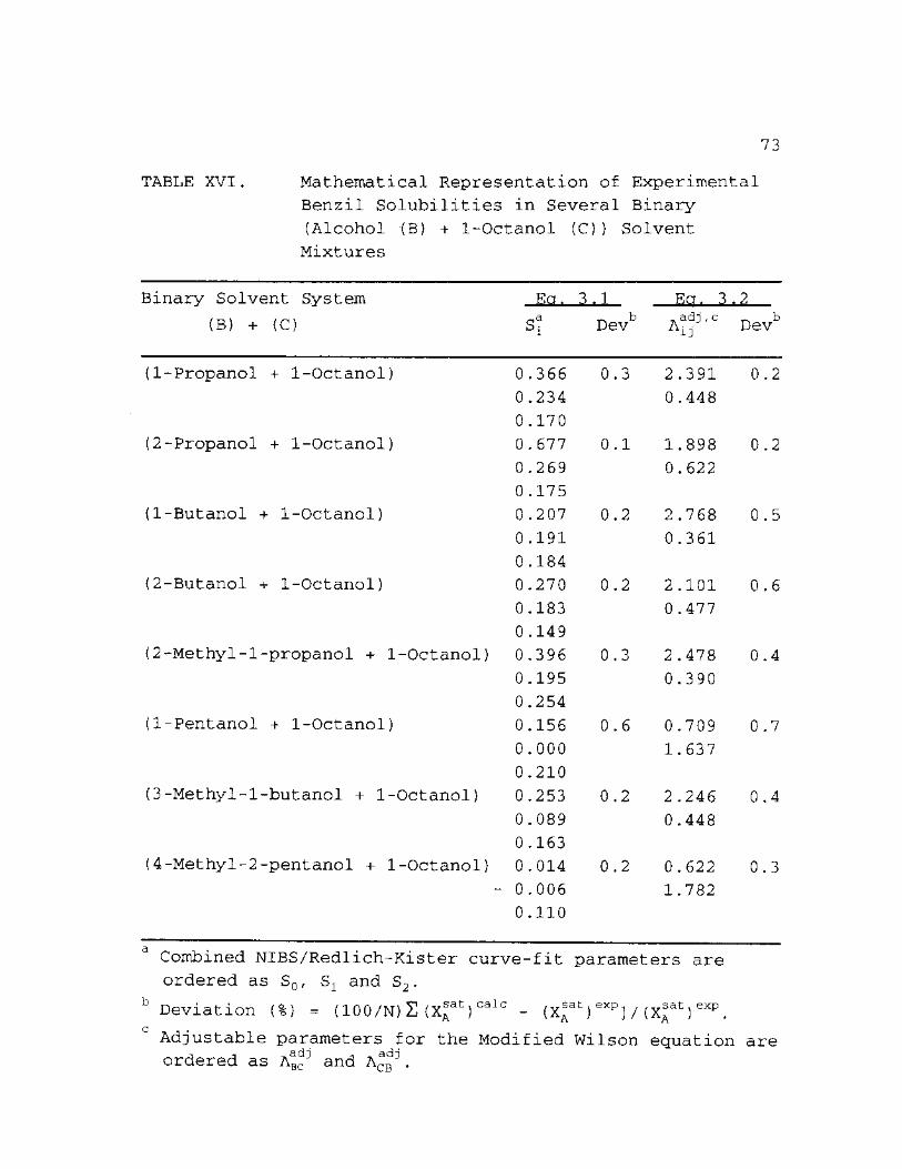
73

TABLE XVI. Mathematical Representation of Experimental Benzil Solubilities in Several Binary (Alcohol (B) + 1-Octanol (C)) Solvent Mixtures

Binary Solvent System

(B) + (C) 3 ,I

s. Dev

Eg, 3,2 _ adj,c _ b A J J Dev

(1 -Propanol + 1-Octanol) 0.366 0 .3 2 .391 0 .2 0.234 0 .448 0.170

(2 -Propanol + 1-Octanol) 0.677 0 .1 1 .898 0 .2 0.269 0 .622 0.175

(1 -Butanol + 1-Octanol) 0.207 0 .2 2 .768 0 .5 0.191 0 .361 0.184

(2 -Butanol + 1-Octanol) 0 .270 0 .2 2 .101 0 . 6 0.183 0 .477 0.149

(2 -Methyl-1-propanol + 1-Octanol) 0.396 0 .3 2 .478 0 .4 0.195 0 .390 0.254

(1 -Pentanol + 1-Octanol) 0.156 0 .6 0 .709 0 .7 0.000 1 .637 0.210

(3 -Methyl-1-butanol + 1-Octanol) 0.253 0 .2 2 .246 0 .4 0.089 0 .448 0.163

(4 -Methyl-2-pentanol + 1-Octanol) 0.014 0 .2 0 .622 0 .3 0.006 1 .782 0.110

Combined NIBS/Redlich-Kister curve-fit parameters are ordered as S0, S2 and S2.

Deviation (%) = (100/N) 2 (X®at) calc - (X®at) exp] / (X*at) exp .

Adjustable parameters for the Modified Wilson equation are ordered as AB^ and A ^ .

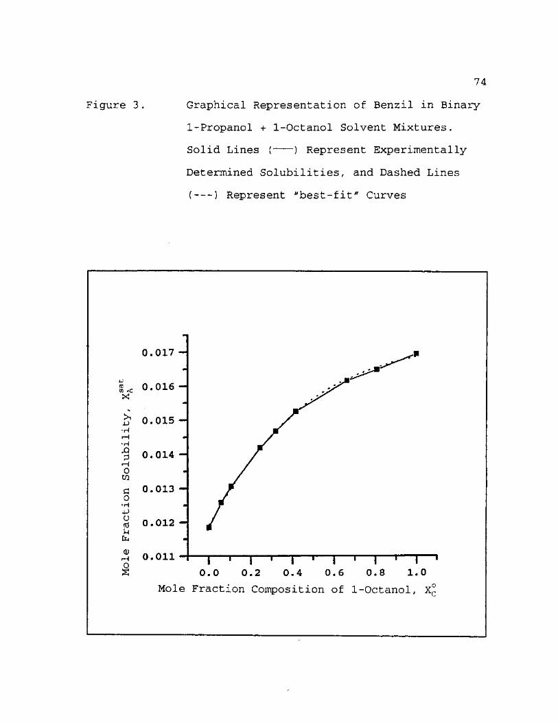
74

Figure 3. Graphical Representation of Benzil in Binary

1-Propanol + 1-Octanol Solvent Mixtures.

Solid Lines ( ) Represent Experimentally

Determined Solubilities, and Dashed Lines

( ) Represent "best-fit" Curves

0.017 -

8* o.016 H X!

>i .u •H r-H

•H 43 3 <—I o C/3 £ o

• H

4J U S-l Ix,

rH 0.011 o s

0.015 -

m

0.014 -

m

0.013 -

m

0.012 -

—| 1 1 1 1 1 1 1 j 1 j 1 0.0 0.2 0.4 0.6 0.8 1.0

Mole Fraction Composition of 1-Octanol, Xp

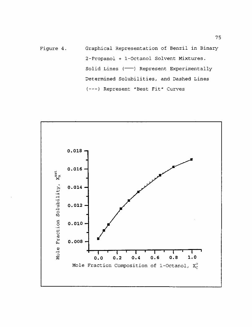
75

Figure 4. Graphical Representation of Benzil in Binary

2-Propanol + 1-Octanol Solvent Mixtures.

Solid Lines ( ) Represent Experimentally-

Determined Solubilities, and Dashed Lines

( ) Represent "Best Fit" Curves

0.018 -

m

1 1 0.016 -

(0 m

4J •H rH •H

0.014 -

rQ 3 rH 0 w

0.012 -

m / d o •H 4J O cd

0.010 -

m / u (X4 0.008 -

Q) 1—i O s

i • i • i • i • i • » 1

0.0 0.2 0.4 0.6 0.8 1.0

Mole Fraction Composition of 1-Octanol, x£

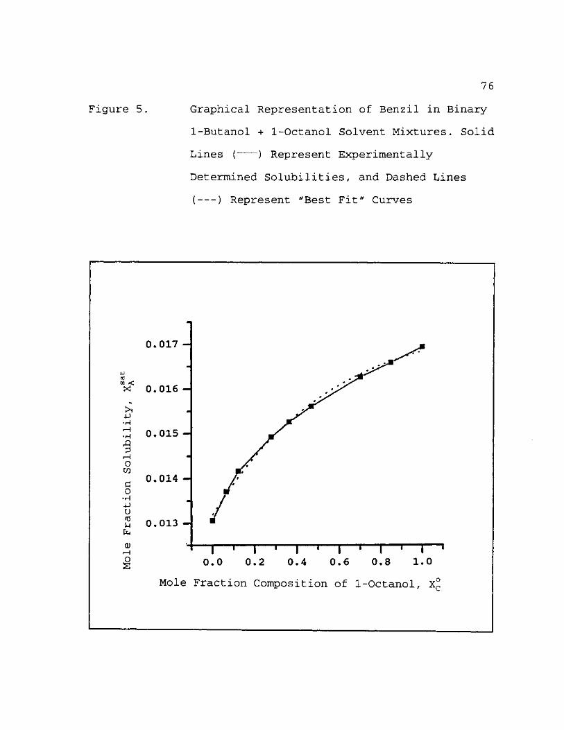
Figure 5.

76

Graphical Representation of Benzil in Binary

1-Butanol + 1-Octanol Solvent Mixtures. Solid

Lines ( ) Represent Experimentally

Determined Solubilities, and Dashed Lines

( ) Represent "Best Fit" Curves

0.017 -

0.016 -

0.015 -

0.014 -

0.013 -

o 2

i — « — i — « — i — « — i — • — i — « — r ~ » 0.0 0.2 0.4 0.6 0.8 1.0

Mole Fraction Composition of 1-Octanol, X~

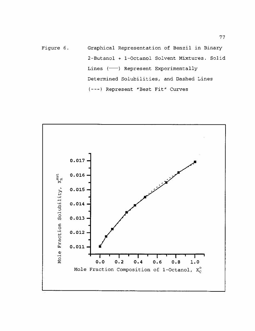
Figure 6.

77

Graphical Representation of Benzil in Binary

2-Butanol + 1-Octanol Solvent Mixtures. Solid

Lines { ) Represent Experimentally

Determined Solubilities, and Dashed Lines

( ) Represent "Best Fit" Curves

-U (0 CO < X

>i 4J •H »—I rQ P

rH O CO a o

•H iJ U (d u

a) rH o s

0.017 -m

0.016 -m

0.015 -m

0.014 -m

0.013 -m

0.012 -

0.011 -n — « — i — 1 — i — • — i — 1 — i — » — i — * 0.0 0.2 0.4 0.6 0.8 1.0

Mole Fraction Composition of 1-Octanol,

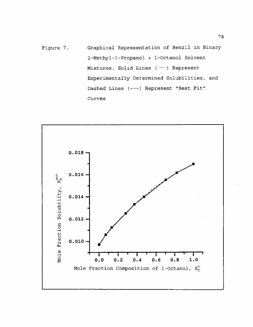
Figure 7

78

Graphical Representation of Benzil in Binary

2-Methyl-1-Propanol + 1-Octanol Solvent

Mixtures. Solid Lines ( ) Represent

Experimentally Determined Solubilities, and

Dashed Lines ( ) Represent "Best Fit"

Curves

<C w <c X

>i 4J •H t—I •HI A P r—I o U) a o •H 4J U (d u PLI CL) <—I o £

0 . 0 1 8 - i

0.016

0.014 -

0.012 -

0.010

—| 1 | ' | 1 | 1 | ' I ' 0.0 0.2 0.4 0.6 0.8 1.0

Mole Fraction Composition of 1-Octanol, Xp

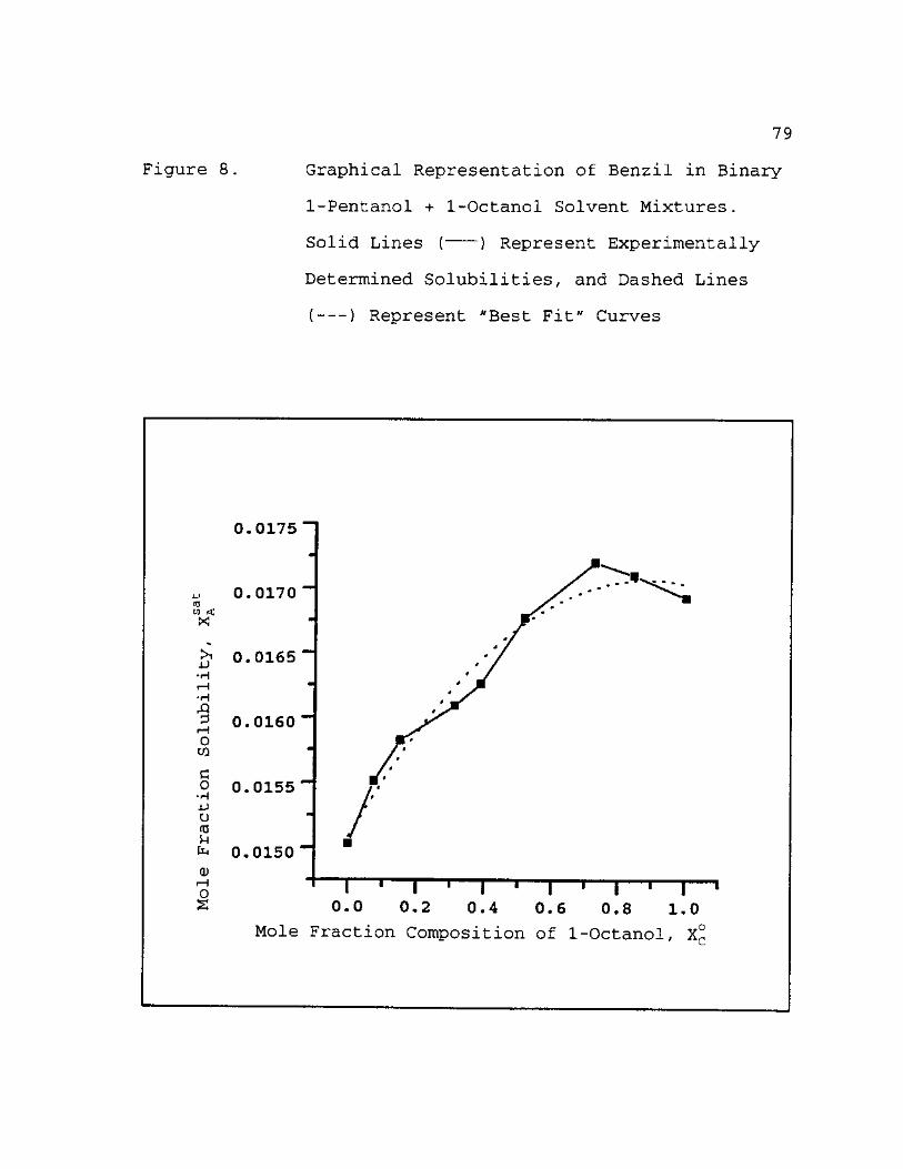
79

Figure 8. Graphical Representation of Benzil in Binary

1-Pentanol + 1-Octanol Solvent Mixtures.

Solid Lines ( ) Represent Experimentally-

Determined Solubilities, and Dashed Lines

( ) Represent "Best Fit" Curves

0.0175

0.0170 (0

W < X

>1 XJ •H rH •H & 3 rH o CO a o

•H 4J U (d u

a) rH o S

0.0165

0.0160

0.0155

0.0150

"1 1 I • 1 1 1 ' 1 « 1 ' 0.0 0.2 0.4 0.6 0.8 1.0

Mole Fraction Composition of 1-Octanol, X(

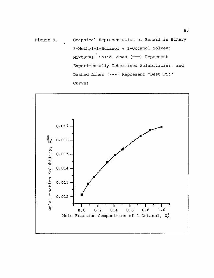
80

Figure 9 Graphical Representation of Benzil in Binary

3-Methyl-1-Butanol + 1-Octanol Solvent

Mixtures. Solid Lines ( ) Represent

Experimentally Determined Solubilities, and

Dashed Lines ( ) Represent "Best Fit"

Curves

a o

•H jj u (0 u ti <u i—i o S

0.017 -

0.016 -

0.015 -•U •H rH •H A -H 0.014 H w

0.013 -

0.012 -

"1 ' 1 ' 1 1 1 • 1 1 1 1

0.0 0.2 0.4 0.6 0.8 1.0

Mole Fraction Composition of 1-Octanol, x£

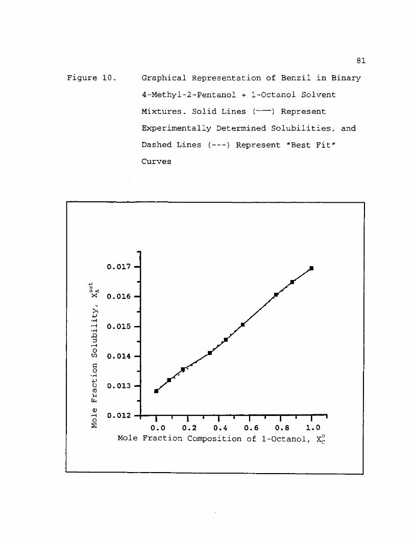
81

Figure 10. Graphical Representation of Benzil in Binary

4-Methyl-2-Pentanol + 1-Octanol Solvent

Mixtures. Solid Lines ( ) Represent

Experimentally Determined Solubilities, and

Dashed Lines ( ) Represent "Best Fit"

Curves

o u3 c o

• H 4-> U (d u Ixi CD i—I o a

0.017 -

u (0 w <C X 0.016-

4J •H 0.015 H

p

0.014 -

0.013 -

0.012 —| 1 J 1 1 1 1 1 1 1 1 1 0.0 0.2 0.4 0.6 0.8 1.0

Mole Fraction Composition of 1-Octanol, X~

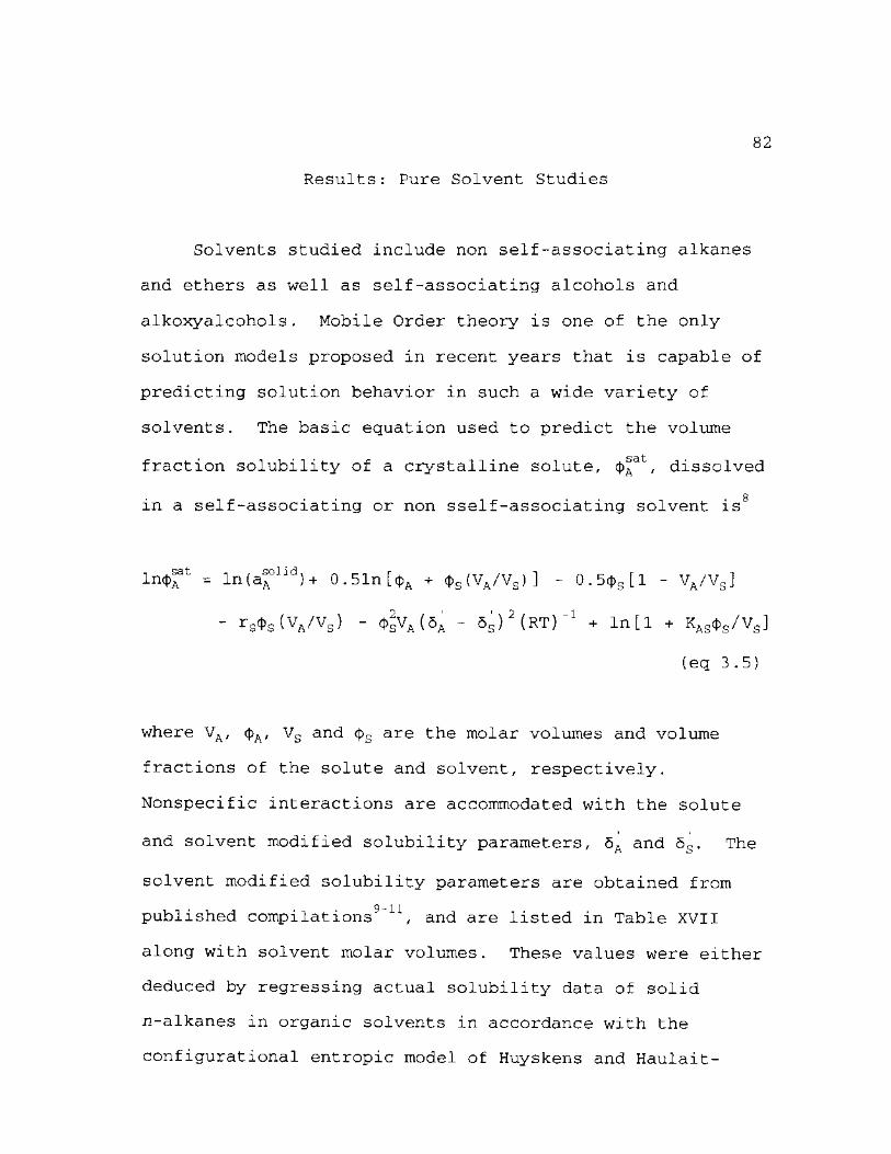
82

Results: Pure Solvent Studies

Solvents studied include non self-associating alkanes

and ethers as well as self-associating alcohols and

alkoxyalcohols. Mobile Order theory is one of the only

solution models proposed in recent years that is capable of

predicting solution behavior in such a wide variety of

solvents. The basic equation used to predict the volume

fraction solubility of a crystalline solute, c|>Aat, dissolved

in a self-associating or non sself-associating solvent is

l n ^ = ln(aA°lid) + 0.51n|>A + <t>s(VA/Vs)] - 0. 5<J>S [ 1 - VA/VS]

- rs<J)s (VA/VS) - 4>sVa(5a " 5 s)2( r t) _ 1 + ln[l + Kasc|>s/Vs]

(eq 3.5)

where VA, <J)A, Vs and <|>s are the molar volumes and volume

fractions of the solute and solvent, respectively.

Nonspecific interactions are accommodated with the solute

and solvent modified solubility parameters, 5A and 5S. The

solvent modified solubility parameters are obtained from

published compilations9"11, and are listed in Table XVII

along with solvent molar volumes. These values were either

deduced by regressing actual solubility data of solid

n-alkanes in organic solvents in accordance with the

configurational entropic model of Huyskens and Haulait-

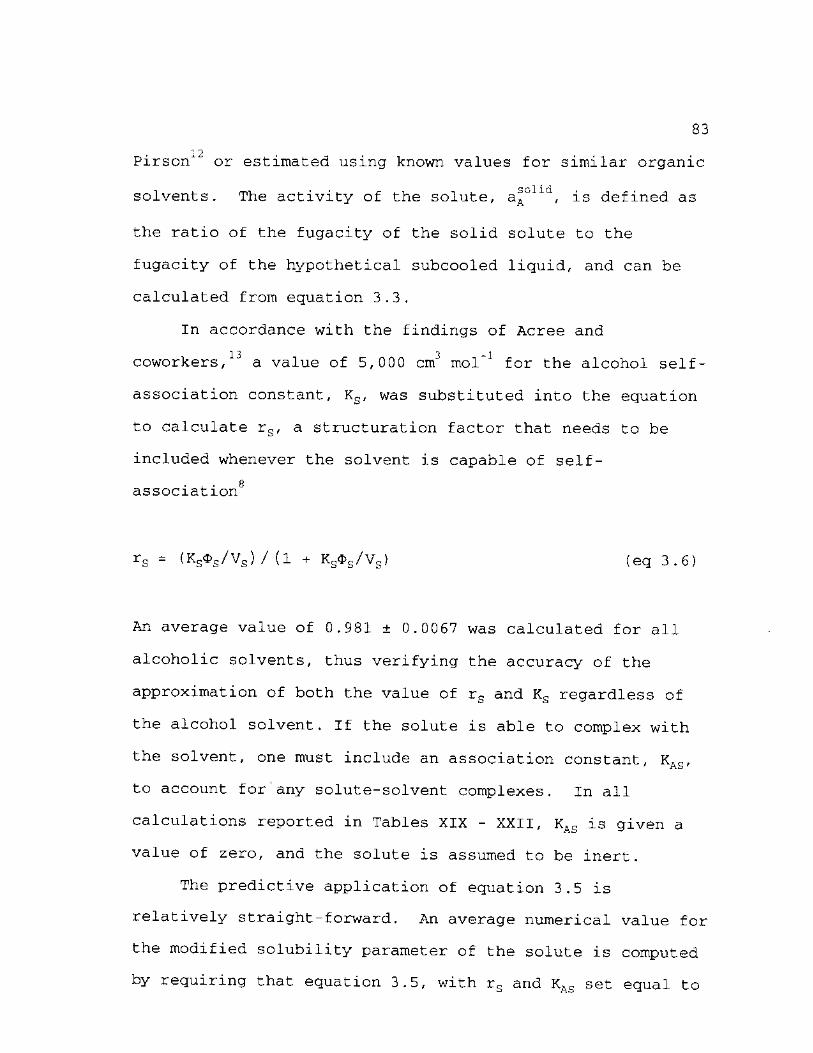
83

12

Pirson or estimated using known values for similar organic

solvents. The activity of the solute, aAolld, is defined as

the ratio of the fugacity of the solid solute to the

fugacity of the hypothetical subcooled liquid, and can be

calculated from equation 3.3.

In accordance with the findings of Acree and 13 3 - 1

coworkers, a value of 5,000 cm mol for the alcohol self-

association constant, Ks, was substituted into the equation

to calculate rs, a structuration factor that needs to be

included whenever the solvent is capable of self-g

association

rs — (Ks4>s/Vs) / (l + K s $ s / V g ) (eq 3.6)

An average value of 0.981 ± 0.0067 was calculated for all

alcoholic solvents, thus verifying the accuracy of the

approximation of both the value of rs and Ks regardless of

the alcohol solvent. If the solute is able to complex with

the solvent, one must include an association constant, KAS,

to account for any solute-solvent complexes. In all

calculations reported in Tables XIX - XXII, KAS is given a

value of zero, and the solute is assumed to be inert.

The predictive application of equation 3.5 is

relatively straight-forward. An average numerical value for

the modified solubility parameter of the solute is computed

by requiring that equation 3.5, with rs and KAS set equal to

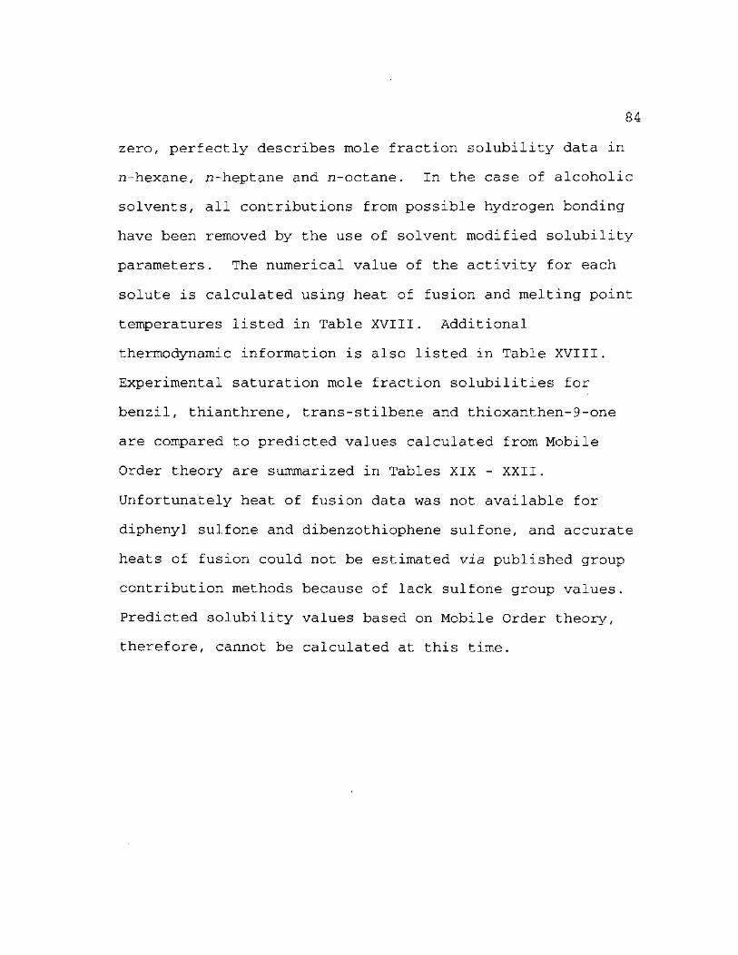
84

zero, perfectly describes mole fraction solubility data in

n-hexane, zi-heptane and n-octane. In the case of alcoholic

solvents, all contributions from possible hydrogen bonding

have been removed by the use of solvent modified solubility

parameters. The numerical value of the activity for each

solute is calculated using heat of fusion and melting point

temperatures listed in Table XVIII. Additional

thermodynamic information is also listed in Table XVIII.

Experimental saturation mole fraction solubilities for

benzil, thianthrene, trans-stilbene and thioxanthen-9-one

are compared to predicted values calculated from Mobile

Order theory are summarized in Tables XIX - XXII.

Unfortunately heat of fusion data was not available for

diphenyl sulfone and dibenzothiophene sulfone, and accurate

heats of fusion could not be estimated via published group

contribution methods because of lack sulfone group values.

Predicted solubility values based on Mobile Order theory,

therefore, cannot be calculated at this time.

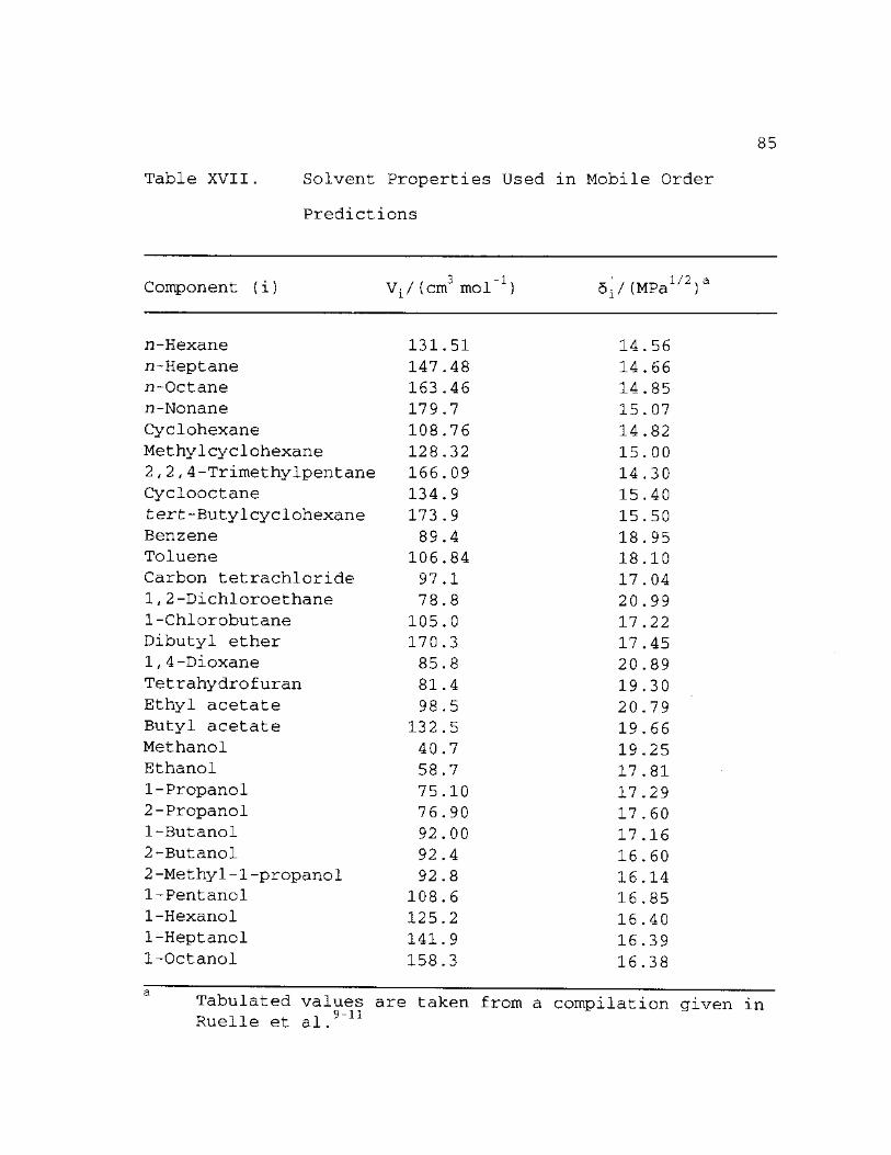
85

Table XVII Solvent Properties Used in Mobile Order

Predictions

Component (i) Vi/ (cm3 mol 1) 5 / (MPa1/2)a

n-Hexane 131 .51 14 .56 n-Heptane 147 .48 14 . 66 n-Octane 163 .46 14 .85 n-Nonane 179 .7 15 .07 Cyclohexane 108 .76 14 .82 Methylcyclohexane 128 .32 15 .00 2,2,4-Trimethylpentane 166 .09 14 .30 Cyclooctane 134 .9 15 .40 fcerfc-Butylcyclohexane 173 .9 15 .50 Benzene 89 .4 18 .95 Toluene 106 .84 18 .10 Carbon tetrachloride 97 .1 17 .04 1,2-Dichloroethane 78 .8 20 .99 1-Chlorobutane 105 .0 17 .22 Dibutyl ether 170 .3 17 .45 1,4-Dioxane 85 .8 20 .89 Tetrahydrofuran 81 .4 19 .30 Ethyl acetate 98 .5 20 .79 Butyl acetate 132 .5 19 .66 Methanol 40 .7 19 .25 Ethanol 58 .7 17 .81 1-Propanol 75 .10 17 .29 2-Propanol 76 .90 17 .60 1-Butanol 92 .00 17 .16 2-Butanol 92 .4 16 .60 2-Methyl-l-propanol 92 .8 16 .14 1-Pentanol 108 .6 16 .85 1-Hexanol 125 .2 16 .40 1-Heptanol 141 .9 16 .39 1-Octanol 158 .3 16 .38

Tabulated values are taken from a compilation given in Ruelle et al. 9-11

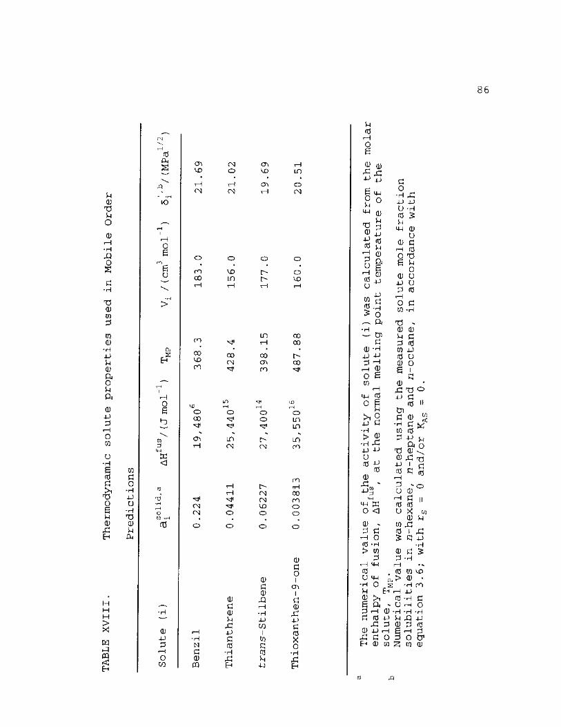
86

u CD T5 U O

CD rH *H A o g

a

•H

T5 cd (0 3 co CD -H 4J U CD &

O U 0^

CD 4J 3 r—I o co

0 •H g

03 fi

£ 1 5H CD

Eh

> X

W J P Q g

CO a o *H JJ

U - H T5 CD U 04

fd £

KD

8 n g U

cu

o g

w 3 M-) IU <1

(0

TJ -H rH o CO -H

fd

CM o\ rH UD O VX> LO

t—i n—1 CT) O CM CM t—1 CM

O o o o • • • •

00 KD l> o 00 if) [> rH rH rH rH

CO if) 00 CO rH 00

00 00 00 l> UD CM (J\ 00 ro ro

LD VD V£> r-i T—1 T 1 o o o o 00 o LD

LD V H.

o\ in o LO rH CM CM CO

ro T—1 l> rH rH CM 00

CM ro CM KO o CM O O o

• • • •

O O O o

CD a (D

CD XI V a <—1

*H CD •H u 4->

CD rC CO

CD >—I 4J 1 4J -H a CO

N fd CJ rH a •H fd O CD & CO PQ EH 4J

CD a 0 1 CP> I a CD rC 4J a fd x o -H ,a E H

u fd rH o 6

5 ^

-^13

6 4-1 c9 o

T5 CD 4J fd 1—I 3 u I—I fd a

CO (d £

o

(d

0

-U

m-I in o <j

CD 3

<d >

a o •H rCj -U 4J

CD u 3 4J (d u CD a &

0 •U

4J a *rH o a

— 0) a

a) *H 4J 4J

M s o g CO

I—I M-j fd

0 B

"> a; -H ,C 4-) 4->

•rH £

CD

O • fd M M-j CD

a a fd

O T5 e n

o cd a 4J o 3 fd rH o a CO -H

T5 -CD CD

a fd 4J

II

CO <

a o -H CO 3

rH UH fd u ^ a, •H O s Jh EH -a> >i g a -3 <-H CD • a fd -u

& 3 CD 4J r-H rC a o Eh CD CO

fd O CD O g «

d CD £1 T5 O -p a

fd D) C CD •h a co fd 3 4J t,

rW ^ O T5 CD CD rd 4-> I £

« 13 r~"I 3 - o o a) rH C || 03 (0 u X

CD CO £ (0 I A £ q .u

• H cd a £ 3 -H

w

fd CO > CD •

•H ro H 4J fd -H CJ O i—10 •H -H *H U rQ 4J CD 3 fd £ rH ^ 3 o c £ w <D

87

Results: Benzil Study

» 1/2 An average value of 5A = 21.69 MPa was calculated

' 1/2 from benzil solubility data in n-hexane (5A = 21.70 MPa ),

ii-heptane (5A = 21.64 MPa1/2), and rz-octane (5A = 21.72

1/2

MPa ). The molar volume of the hypothetical subcooled

liquid solute, VA = 183 cm3 mol"1 was estimated from the

density of the liquid at 102 °C6 and the coefficient of

thermal expansion for benzophenone calculated over the

temperature range of 50-95 °C.17 Table XIX summarizes the

predictive ability of Mobile Order theory for the thirty

different organic solvents for which both benzil solubility

data and modified solubility parameters could be found.

Examination of Table XIX reveals an average absolute

deviation of circa 21 % for nonassociating solvents, with

larger deviations, 44 %, in alcoholic solvents. Had an

ideal system been assumed, the predictive mole fraction

solubility would have been (XAat)ld = (aA

olld)ld = 0.224 for

each solvent. The ideal solution solubility approximation

corresponds to an average absolute deviation of 1,500 %

between the predicted and observed values.

Thianthrene Study

An average value for the thianthrene modified

88

1/2

solubility parameter, 21.02 MPa , is computed from the

three values obtained in n-hexane, n-heptane, n-octane:

21.00 MPa1/2, 21.00 MPa1/2, and 21.05 MPa1/2, respectively. A 3 - 1 .

value of 156.0 cm mol was used m Mobile Order 18

calculations. Table XX summarizes the predictive ability

of Mobile Order theory for the twenty different organic

solvents for which both thianthrene solubility data and

modified solubility parameters were available. Examination

of Table XX reveals an average absolute deviation of circa

58 % for all solvents studied, and an average deviation of

83 % for alcohol solvents. Had an ideal system been

assumed, there would have been an average absolute deviation

of 1,940 % between the predicted mole fraction solubility of

(XAat)ld = (aA

olld)ld = 0.04411 for each solvent and the

observed values.

trans-Stilbene Study

« 1/2 An average numerical value of 5A = 19.69 MPa is

computed from mole fraction solubility data in n-hexane

(5a = 19.78 MPa1/2), n-heptane (5A = 19.68 MPa

172), and

n-octane (5A = 19.60 MPa1/2) . The molar volume was taken to

3 -1 19

have the value of 177.0 cm mol . Table XXI summarizes

the predictive ability of Mobile Order theory for the twenty

different organic solvents for which both trans-stilbene

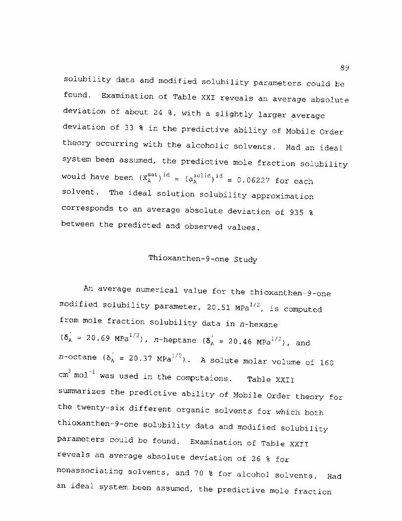
89

solubility data and modified solubility parameters could be

found. Examination of Table XXI reveals an average absolute

deviation of about 24 %, with a slightly larger average

deviation of 33 % in the predictive ability of Mobile Order

theory occurring with the alcoholic solvents. Had an ideal

system been assumed, the predictive mole fraction solubility

would have been (xfV d = (a.Tlid)id = 0.06227 for each

solvent. The ideal solution solubility approximation

corresponds to an average absolute deviation of 935 %

between the predicted and observed values.

Thioxanthen-9-one Study

An average numerical value for the thioxanthen-9-one

modified solubility parameter, 2 0.51 MPa1/2, is computed

from mole fraction solubility data in n-hexane

(5a = 20.69 MPa1/2), n-heptane (5A = 20.46 MPa

1/2) , and

^-octane (5A = 20.37 MPa1/2) . A solute molar volume of 160

cm mol was used in the computaions. Table XXII

summarizes the predictive ability of Mobile Order theory for

the twenty-six different organic solvents for which both

thioxanthen-9-one solubility data and modified solubility

parameters could be found. Examination of Table XXII

reveals an average absolute deviation of 26 % for

nonassociating solvents, and 7 0 % for alcohol solvents. Had

an ideal system been assumed, the predictive mole fraction

90

solubility would have been (X^at)ld = (a^olld)ld = 0.003813 for

each solvent. The ideal solution solubility approximation

corresponds to an average absolute deviation of 42 0 %

between the predicted and observed values.

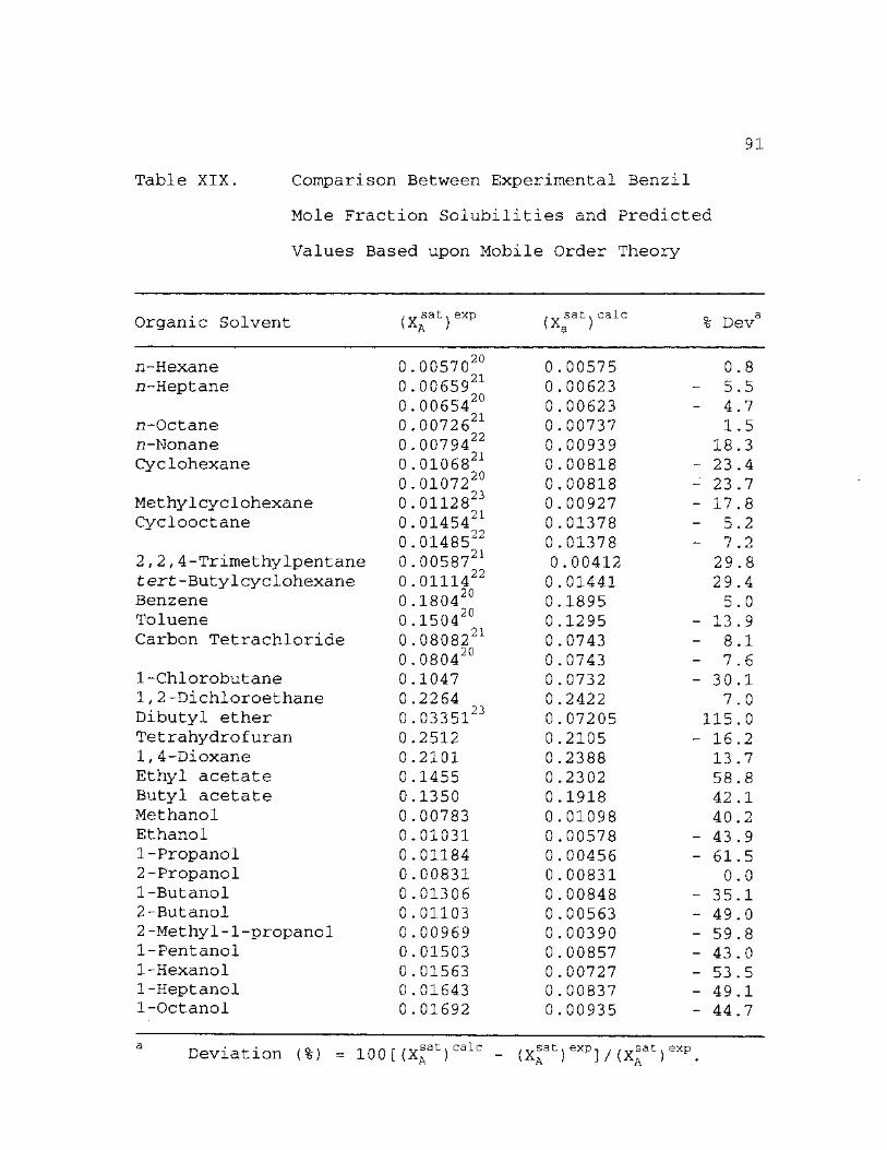
Table XIX. Comparison Between Experimental Benzil

Mole Fraction Solubilities and Predicted

Values Based upon Mobile Order Theory

91

Organic Solvent (XAsat)exp (X; sat * calc a ' % Deva

n-Hexane 0.0057020

0.0065921

0.0065420

0.0072621

0.0079422

0.0106821

0.0107220

0.0112823

0.0145421

0.0148522

0. 00575 0 .8 n-Heptane

0.0057020

0.0065921

0.0065420

0.0072621

0.0079422

0.0106821

0.0107220

0.0112823

0.0145421

0.0148522

0. 00623 - 5 .5 0.0057020

0.0065921

0.0065420

0.0072621

0.0079422

0.0106821

0.0107220

0.0112823

0.0145421

0.0148522

0. 00623 - 4 .7 .n-Octane

0.0057020

0.0065921

0.0065420

0.0072621

0.0079422

0.0106821

0.0107220

0.0112823

0.0145421

0.0148522

0. 00737 1 .5 n-Nonane

0.0057020

0.0065921

0.0065420

0.0072621

0.0079422

0.0106821

0.0107220

0.0112823

0.0145421

0.0148522

0. 00939 18 .3 Cyclohexane

0.0057020

0.0065921

0.0065420

0.0072621

0.0079422

0.0106821

0.0107220

0.0112823

0.0145421

0.0148522

0. 00818 - 23 .4

0.0057020

0.0065921

0.0065420

0.0072621

0.0079422

0.0106821

0.0107220

0.0112823

0.0145421

0.0148522

0. 00818 - 23 .7 Methyleyelohexane

0.0057020

0.0065921

0.0065420

0.0072621

0.0079422

0.0106821

0.0107220

0.0112823

0.0145421

0.0148522

0. 00927 - 17 .8 Cyclooctane

0.0057020

0.0065921

0.0065420

0.0072621

0.0079422

0.0106821

0.0107220

0.0112823

0.0145421

0.0148522 0. 01378 - 5 .2

0.0057020

0.0065921

0.0065420

0.0072621

0.0079422

0.0106821

0.0107220

0.0112823

0.0145421

0.0148522 0. 01378 - 7 .2 2,2,4-Trimethylpentane 0.0058721

0.0111422

0.180420

0 .00412 29 .8 tert-Butyleyelohexane

0.0058721

0.0111422

0.180420 0. 01441 29 .4

Benzene

0.0058721

0.0111422

0.180420 0. 1895 5 .0 Toluene 0.150420 0. 1295 - 13 .9 Carbon Tetrachloride 0.0808221

0.080420 0. 0743 - 8 .1 0.0808221

0.080420 0. 0743 - 7 .6 1-Chlorobutane 0.1047 0. 0732 - 30 .1 1,2-Dichloroethane 0.2264 0. 2422 7 .0 Dibutyl ether 0.0335123 0. 07205 115 .0 Tetrahydrofuran 0.2512 0. 2105 - 16 .2 1,4-Dioxane 0.2101 0. 2388 13 .7 Ethyl acetate 0.1455 0. 2302 58 .8 Butyl acetate 0.1350 0. 1918 42 .1 Methanol 0.00783 0. 01098 40 .2 Ethanol 0.01031 0. 00578 - 43 .9 1-Propanol 0.01184 0. 00456 - 61 .5 2-Propanol 0.00831 0. 00831 0 .0 1-Butanol 0.01306 0. 00848 - 35 .1 2-Butanol 0.01103 0. 00563 - 49 .0 2-Methyl-1-propanol 0.00969 0. 00390 - 59 .8 1-Pentanol 0.01503 0. 00857 - 43 .0 1-Hexanol 0.01563 0. 00727 - 53 .5 1-Heptanol 0.01643 0. 00837 - 49 .1 1-Octanol 0.01692 0. 00935 - 44 .7

a Deviation (%) = 100 [ (X^at) calc - / yr sat 1 \ Aa , iexp]/(xft) iexp.

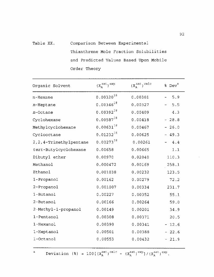
Table XX.

92

Comparison Between Experimental

Thianthrene Mole Fraction Solubilities

and Predicted Values Based Upon Mobile

Order Theory

Organic Solvent . v sat, exp v A a ; , v sat v calc ( ) Dev

n-Hexane 0.0032018 0. 00301 - 5 .9

n-Heptane 0.0034618 0. 00327 - 5 .5

n-Octane 0.0039218 0. 00409 4 .3

Cyclohexane 0.0058718 0. 00418 - 28 .8

Methylcyclohexane 0.0063118 0. 00467 - 26 .0

Cyclooctane 0.0123218 0. 00625 - 49 .3

2,2,4-Trimethylpentane 0.0027318 0 .00261 - 4 .4

fcerfc-Butylcyclohexane 0.00658 0. 00665 1 .1

Dibutyl ether 0.00970 0. 02040 110 .3

Methanol 0.000472 0. 00169 258 .1

Ethanol 0.001038 0. 00232 123 .5

1-Propanol 0.00162 0. 00279 72 .2

2-Propanol 0.001007 0. 00334 231 .7

1-Butanol 0 .00227 0. 00352 55 .1

2-Butanol 0.00166 0. 00264 59 .0

2-Methyl-1-propanol 0.00149 0. 00201 34 .9

1-Pentanol 0.00308 0. 00371 20 .5

1-Hexanol 0.00390 0. 00341 - 12 .6

1-Heptanol 0.00501 0. 00388 - 22 .6

1-Octanol 0.00553 0. 00432 - 21 .9

a Deviation (%) = 100 [ (X^at)calc - (Xjat )exp]/(xft) exp

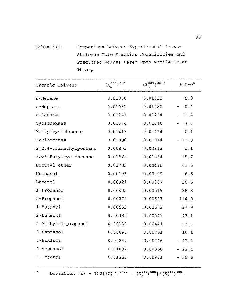
93

Table XXI. Comparison Between Experimental trans-

Stilbene Mole Fraction Solubilities and

Predicted Values Based Upon Mobile Order

Theory

Organic Solvent , sat. exp ( A A ) (X sat. calc % Dev

n-Hexane 0 .00960 0 .01025 6 .8

n-Heptane 0 .01085 0 .01080 - 0 .4

n-Octane 0 .01241 0 .01224 - 1 .4

Cyclohexane 0 .01374 0 .01316 - 4 .3

Me t hy 1 cy c 1 ohexan e 0 .01413 0 .01414 0 .1

Cyclooctane 0 .02080 0 .01814 - 12 .8

2,2,4-Trimethylpentane 0 .00803 0 .00812 1 .1

tert-Butylcyclohexane 0 .01570 0 .01864 18 .7

Dibutyl ether 0 .02783 0 .04498 61 .6

Methanol 0 .00196 0 .00209 6 .5

Ethanol 0 .00321 0 .00387 20 .5

1-Propanol 0 .00403 0 .00519 28 .8

2-Propanol 0 .00279 0 .00597 114 .0

1-Butanol 0 .00533 0 .00682 27 .9

2-Butanol 0 .00382 0 .00547 43 .1

2-Methyl-1-propanol 0 .00330 0 .00441 33 .7

1-Pentanol 0 .00691 0 .00761 10 .1

1-Hexanol 0 .00841 0 .00746 - 11 .4

1-Heptanol 0 .01092 0 .00858 - 21 .4

1-Octanol 0 .01251 0 .00961 - 50 . 6

Deviation (%) = 100 [ (Xlat)calc ixfat)exp]/(xfat)exp.

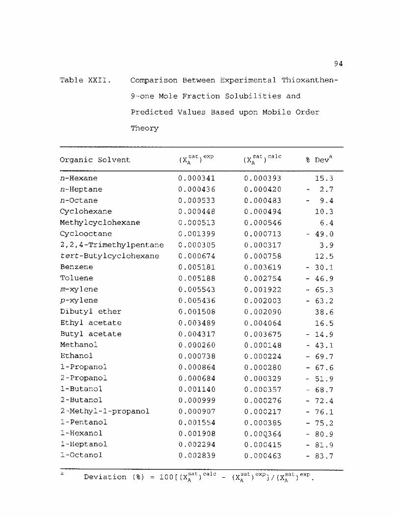
94

Table XXII. Comparison Between Experimental Thioxanthen-

9-one Mole Fraction Solubilities and

Predicted Values Based upon Mobile Order

Theory

Organic Solvent s a t) e x p , sat» calc I Aa ) Dev

zi-Hexane 0. .000341 0. .000393 15, .3 n-Heptane 0. .000436 0. .000420 - 2. .7

ii-Octane 0. .000533 0. .000483 - 9. .4 Cyclohexane 0. .000448 0. .000494 10. .3 Methylcyclohexane 0, .000513 0. .000546 6, .4 Cyclooctane 0, .001399 0. .000713 - 49. .0 2,2,4-Trimethylpentane 0. .000305 0. .000317 3 . .9 tert-Butylcyclohexane 0, .000674 0, .000758 12 . .5 Benzene 0, .005181 0. .003619 - 30. .1 Toluene 0, .005188 0. .002754 - 46. .9 m-xylene 0, .005543 0. .001922 - 65, .3 p-xylene 0, .005436 0, .002003 - 63, .2 Dibutyl ether 0. .001508 0. .002090 38, .6 Ethyl acetate 0, .003489 0, .004064 16, .5 Butyl acetate 0. .004317 0, .003675 - 14, .9 Methanol 0, .000260 0. .000148 - 43, .1 Ethanol 0, .000738 0, .000224 - 69, .7 1-Propanol 0, .000864 0. .000280 - 67, .6 2-Propanol 0, .000684 0, .000329 - 51, .9 1-Butanol 0, .001140 0. .000357 - 68, .7 2-Butanol 0, .000999 0, .000276 - 72. .4 2-Methyl-1-propanol 0. .000907 0, .000217 - 76, .1 1-Pentanol 0, .001554 0, .000385 - 75, .2 1-Hexanol 0. .001908 0. . 00Q364 - 80. .9 1-Heptanol 0 , .002294 0. .000415 - 81. .9 1-Octanol 0 , .002839 0 , .000463 - 83. .7

Deviation (%) = 100 [ (X*at) calc (xfat)exp ] / (xfat)exp,

95

Solute-Solvent Association Constants

In the hope of developing a purely predictive

expression with no adjustable parameters, I was interested

in investigating the change in the optimized solute-solvent

association constant as the solute changed. Generally only

inert solutes have been studied in complexing and

noncomplexing solvents, or proton donating solutes have been

studied in non self-associating solvents. I was interested

in the ability of electron donor solutes to form hydrogen

bonds with the solvent, and the effect of these hydrogen

bonds on the solute solubility. Clearly, solute-solvent

interactions will affect solute solubility, and a thorough

understanding of these effects will aid the researcher in

both understanding solution behavior and predicting this

behavior.

Initially, I assumed there were no solute-solvent

interactions, and assigned a value of zero to the solute-

solvent association constant, KAS. This assumption provided

reasonable results for nonassociating alkane solvents, with

an average absolute deviation of 12.4 % for the four solutes

for which heat of fusion data was available. However, in

alcohol solvents capable of forming hydrogen bonds with the

solute, the average absolute deviation for the predicted

solubility of the four solutes increases to 57.5 %. In this

case, it appears the assumption that no solute - solvent

96

associations are present in solution is incorrect. Tables

XXIII and XXIV list the optimized solute - solvent

association constants for benzil and thioxanthen-9-one in

each solvent. Numerical values were calculated by

substituting the experimental mole fraction solubilities and

molar volumes into equation 3.5, and then calculating the

one remaining unknown value, KAS. A careful examination of

the molecular structures indicates that it would be possible

for hydrogen bond formation to occur between the alcoholic

hydroxylic OH group and the oxygen lone electron pairs on

benzil and/or thioxanthen-9-one. For calculational

simplicity, only a 1:1 solute - solvent molecular complex is

3 -1

assumed. A negative value of KAS = -1.7 cm mol was

calculated in the case of benzil with 1-propanol, indicating

that any molecular complex formed would be fairly weak. An

experimental uncertainty of ±2 % in the measured mole

fraction leads to a ±20 cm3 mol 1 or so uncertainty in the

calculated value of KAS. Calculation of the small negative

value for an association constant likely is a result of

either a small error in the measured mole fraction

solubility, or a small error in the modified solubility

parameters, 5A and 5S, or the inability of the

- 5s)2(RT) 1 term to accurately describe nonspecific

interactions. Remember that in the case of solutes

dissolved in saturated hydrocarbon solvents, Mobile Order

theory did not perfectly predict the experimental

97

solubility.

Examination of Tables XXIII and XXIV further reveals

that the calculated association constants for presumed

thioxanthen-9-one - alcohol molecular complexes are for the

most part larger than the association constants for the

presumed benzil - alcohol complex. Molecular structure

considerations indicate that the oxygen lone electron pairs

on the thioxanthen-9-one are not as sterically hindered as

those on benzil, where the two bulky phenyl rings hinder the

approach of an alcohol solvent molecule. Additional studies

involving complexing solutes are needed to determine if any

trends in solute - solvent association behavior exist.

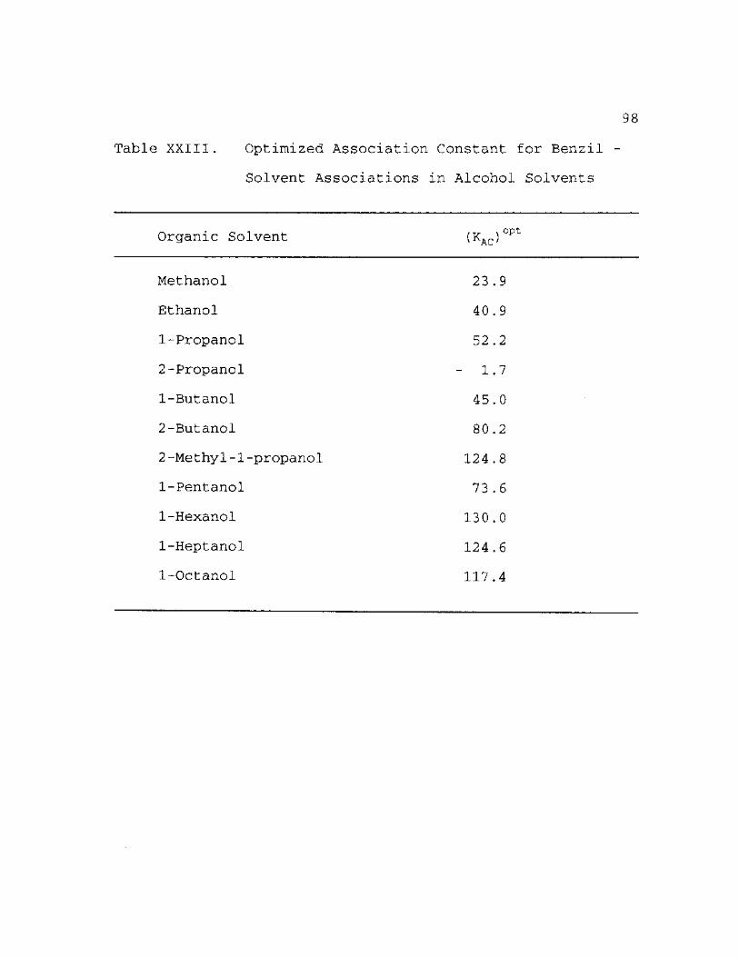
98

Table XXIII. Optimized Association Constant for Benzil -

Solvent Associations in Alcohol Solvents

Organic Solvent (KAc)°Pt

Methanol 23.9

Ethanol 40.9

1-Propanol 52.2

2-Propanol - 1.7

1-Butanol 45.0

2-Butanol 80.2

2-Methyl-1-propanol 124.8

1-Pentanol 73.6

1-Hexanol 130.0

1-Heptanol 124.6

1-Octanol 117.4

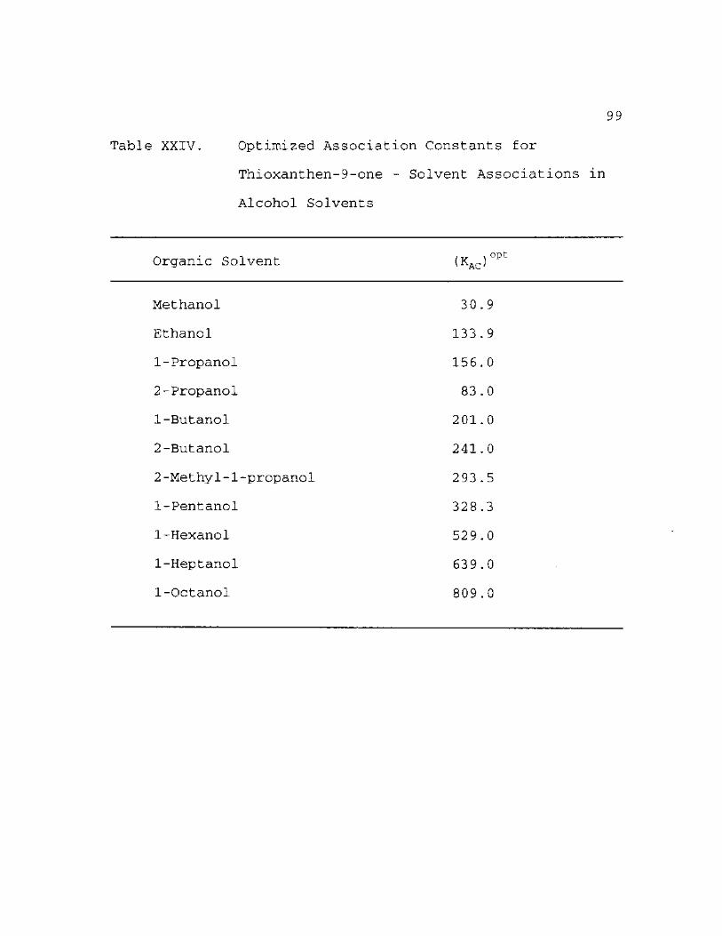
99

Table XXIV. Optimized Association Constants for

Thioxanthen-9-one - Solvent Associations in

Alcohol Solvents

Organic Solvent (KAc)°Pt

Methanol 30.9

Ethanol 133.9

1-Propanol 156.0

2-Propanol 83.0

1-Butanol 201.0

2-Butanol 241.0

2-Methyl-1-propanol 293.5

1-Pentanol 328.3

1-Hexanol 529.0

1-Heptanol 639.0

1-Octanol 809.0

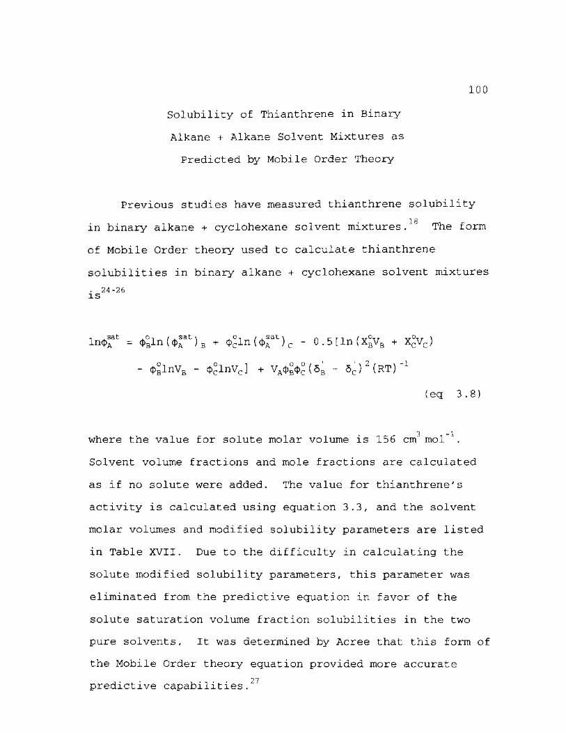
100

Solubility of Thianthrene in Binary

Alkane + Alkane Solvent Mixtures as

Predicted by Mobile Order Theory

Previous studies have measured thianthrene solubility

18

in binary alkane + cyclohexane solvent mixtures. The form

of Mobile Order theory used to calculate thianthrene

solubilities in binary alkane + cyclohexane solvent mixtures . 24-26 IS

ln<Dft = <t>gln (<j) at) B + 0cln(ct>r)c " 0.5[ln(X°VB + X°VC)

- ((>glnVB - 4>clnVc] + VA<{>g(|)Q (5b - 5^) 2 (RT) ~1

(eq 3.8)

3 -1

where the value for solute molar volume is 156 cm mol .

Solvent volume fractions and mole fractions are calculated

as if no solute were added. The value for thianthrene's

activity is calculated using equation 3.3, and the solvent

molar volumes and modified solubility parameters are listed

in Table XVII. Due to the difficulty in calculating the

solute modified solubility parameters, this parameter was

eliminated from the predictive equation in favor of the

solute saturation volume fraction solubilities in the two

pure solvents. It was determined by Acree that this form of

the Mobile Order theory equation provided more accurate 27 predictive capabilities

101

Tables XXV - XXIX compare Mobile Order predictions with

previously determined experimental values of thianthrene

18

solubility in binary alkane + cyclohexane systems for

which pure solvent solubility data is available. Despite

rather large deviations between predicted and experimental

pure solvent solubility values (the largest per cent

deviations are for cyclohexane, -28.8, and cyclooctane,

-49.3), the predictive expression for the solubility of

thianthrene dissolved in a binary alkane + cyclohexane

solvent mixture has an average absolute deviation of only

3.3 %. The reduced deviation results from the fact that the

two solute - solvent nonspecific interaction terms,

d>°2VA ( 5a - 5b)2(RT)_1 and $c2va(5a ~ SCJ^RT)-1, have been

removed from the predictive expression in favor of the

actual experimental solute solubilities in the two pure

solvents. Replacement of the solubility parameter terms

frees the predictive expression from the inherent

limitations of the solubility parameters' inability to

accurately describe nonspecific interactions. Mobile Order

theory consistently under-predicted the solubility of

thianthrene in the binary alkane + cyclohexane systems,

however the deviation was never greater than -7.9 %.

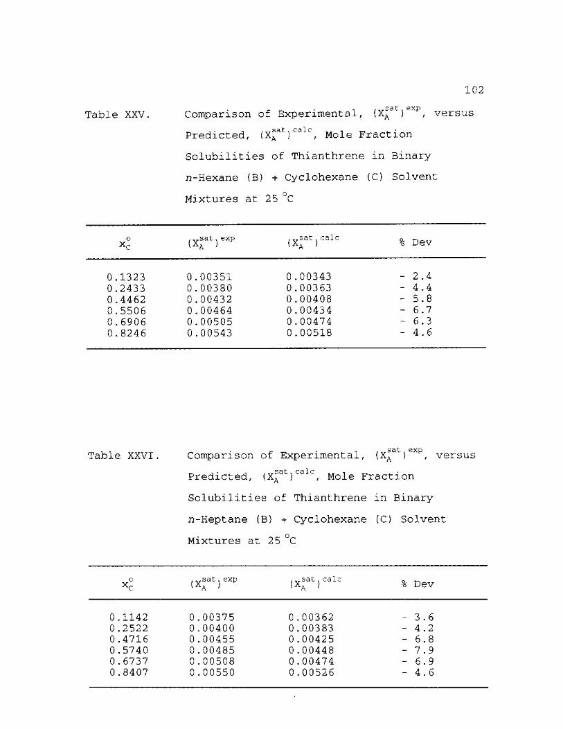
102

Table XXV. Comparison of Experimental, (XA ) , versus

Predicted, (XAat)calc, Mole Fraction

Solubilities of Thianthrene in Binary-

n-Hexane ( B ) + Cyclohexane (C) Solvent

Mixtures at 2 5 °C

i

O u X

. s a t . exp » A >

. v s a t , c a l c ' A ' % Dev

0 . 1 3 2 3 0 . 0 0 3 5 1 0 . 0 0 3 4 3 - 2 . 4

0 . 2 4 3 3 0 . 0 0 3 8 0 0 . 0 0 3 6 3 - 4 . 4

0 . 4 4 6 2 0 . 0 0 4 3 2 0 . 0 0 4 0 8 - 5 . 8

0 . 5 5 0 6 0 . 0 0 4 6 4 0 . 0 0 4 3 4 - 6 . 7

0 . 6 9 0 6 0 . 0 0 5 0 5 0 . 0 0 4 7 4 - 6 . 3

0 . 8 2 4 6 0 . 0 0 5 4 3 0 . 0 0 5 1 8 - 4 . 6

Table XXVI Comparison of Experimental, (XA )

r s a t . c a l c

s a t . exp versus

Predicted, Mole Fraction

Solubilities of Thianthrene in Binary

n-Heptane (B) + Cyclohexane (C) Solvent

Mixtures at 25 °C

O xc , v s a t , exp \ A > /

, s a t , c a l c v ) % Dev

0.1142 0.2522 0.4716 0 .5740 0.6737 0.8407

0.00375 0.00400 0 .00455 0.00485 0.00508 0 .00550

0.00362 0.00383 0.00425 0 .00448 0.00474 0.00526

3.6 4.2 6 . 8 7.9 6.9 4.6

Table XXVII

103

Comparison of Experimental, (XA )

rsat x calc

sat. exp versus

Predicted, (XA ) Mole Fraction

Solubilities of Thianthrene in Binary

n-Octane (B) + Cyclohexane (C) Solvent

Mixtures at 25 °C

xr (x;at)exp . vsat.calc ' A > Dev

0.1472 0.2772 0.3317 0.4994 0.5990 0.6981 0.8556

0.00416 0.00439 0.00447 0.00478 0.00498 0.00517 0.00552

0.00407 0.00423 0.00430 0.00456 0.00475 0.00496 0.00538

2.1 3.1 3.8 4.7 4.8 4.1 2 . 6

Table XXVIII • sat 0xd

Comparison of Experimental, (XA ) , versus

Predicted, (XAat)calc, Mole Fraction

Solubilities of Thianthrene in Binary

Methylcyclohexane (B) + Cyclohexane (C)

Solvent Mixtures at 25 °C

s a t) e x p . sat. calc ' A ' Dev

0.1184 0.2367 0.4375 0 .5401 0.6448 0.8211

0.00626 0.00623 0.00616 0.00610 0.00601 0.00591

0.00627 0.00622 0.00613 0.00608 0.00604 0.00596

0 0 0 0 0 0.8

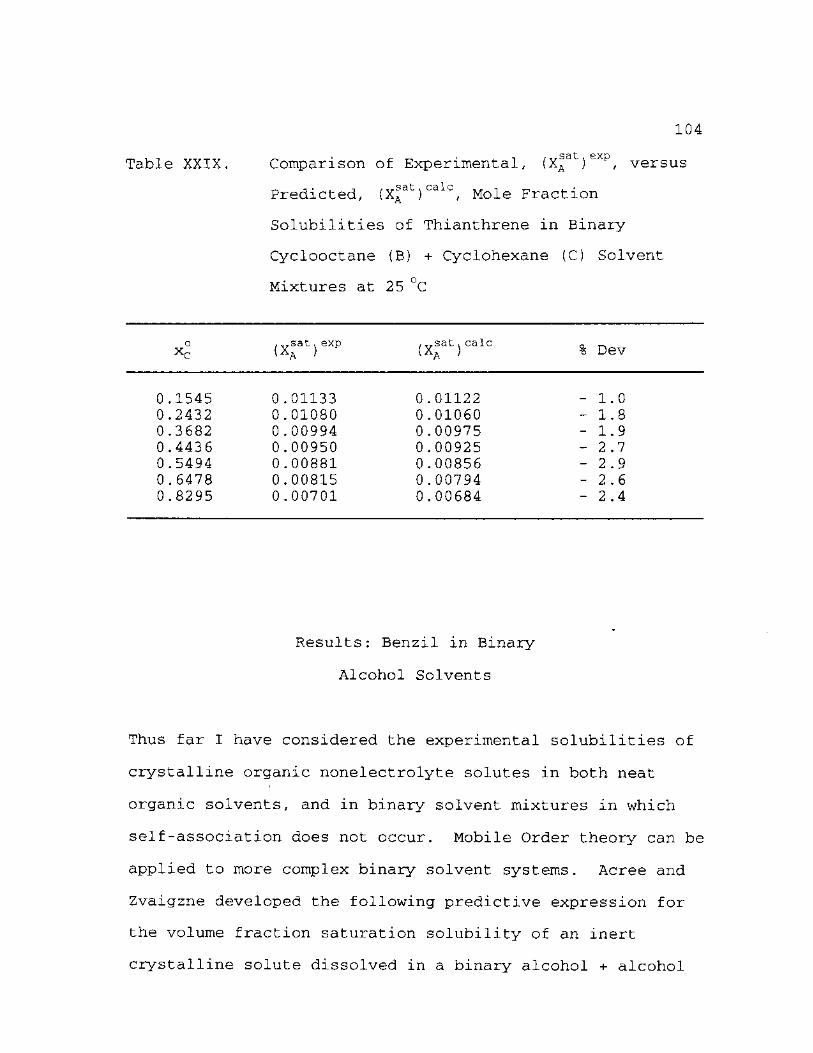
Table XXIX,

104

sat, exp versus Comparison of Experimental, (XA )

Predicted, (x!at)calc, Mole Fraction

Solubilities of Thianthrene in Binary

Cyclooctane (B) + Cyclohexane (C) Solvent

Mixtures at 25 °C

xr , vsat x exp \ )

. sat v calc IXA ) % Dev

0.1545 0.2432 0.3682 0.4436 0.5494 0.6478 0.8295

0.01133 0.01080 0.00994 0.00950 0.00881 0.00815 0.00701

0.01122 0.01060 0.00975 0.00925 0.00856 0.00794 0.00684

1.0 1.8 1.9 2.7 2.9 2.6 2.4

Results: Benzil in Binary

Alcohol Solvents

Thus far I have considered the experimental solubilities of

crystalline organic nonelectrolyte solutes in both neat

organic solvents, and in binary solvent mixtures in which

self-association does not occur. Mobile Order theory can be

applied to more complex binary solvent systems. Acree and

Zvaigzne developed the following predictive expression for

the volume fraction saturation solubility of an inert

crystalline solute dissolved in a binary alcohol + alcohol

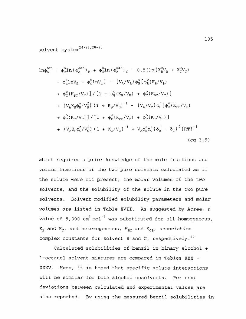
105

, . . 2 4 - 2 6 , 2 8 - 3 0 solvent system

ln^at = «j>°ln(«D®at)B + <D°ln(<t>Aat)c " 0.5[ln(X°VB + X°VC)

- <J>BlnVB - cDclnVc] - (VA/VB) 0° [cJ>B (KB/VB)

+ c { > ° ( K b c / V c ) ] / [ 1 + <t>B(KB/VB) + cf'c ( K b c / V c ) ]

+ (VaKB0B/Vb) (1 + Kb/Vb) _1 - (VA/VC) <Dc [ b (^cB/Vb)

+ <p°(Kc/Vc) ] / [1 + <{>b(Kcb/Vb) + <j>°(Kc/Vc)]

+ (VAKc(t>c/Vc) (1 + Kc/Vc)_1 + VA<J)Bc|)c (5b - 5^)

2 (RT)"1

(eq 3.9)

which requires a prior knowledge of the mole fractions and

volume fractions of the two pure solvents calculated as if

the solute were not present, the molar volumes of the two

solvents, and the solubility of the solute in the two pure

solvents. Solvent modified solubility parameters and molar

volumes are listed in Table XVII. As suggested by Acree, a

3 -1 value of 5,000 cm mol was substituted for all homogeneous,

Kb and Kc, and heterogeneous, KBC and KCB, association

2 6

complex constants for solvent B and C, respectively.

Calculated solubilities of benzil in binary alcohol +

1-octanol solvent mixtures are compared in Tables XXX -

XXXV. Here, it is hoped that specific solute interactions

will be similar for both alcohol cosolvents. Per cent

deviations between calculated and experimental values are

also reported. By using the measured benzil solubilities in

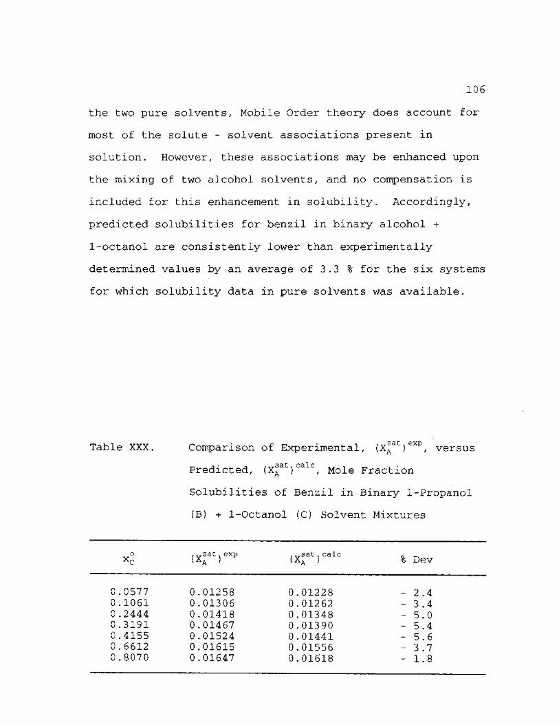
106

the two pure solvents, Mobile Order theory does account for

most of the solute - solvent associations present in

solution. However, these associations may be enhanced upon

the mixing of two alcohol solvents, and no compensation is

included for this enhancement in solubility. Accordingly,

predicted solubilities for benzil in binary alcohol +

1-octanol are consistently lower than experimentally

determined values by an average of 3.3 % for the six systems

for which solubility data in pure solvents was available.

Table XXX. Comparison of Experimental, (X^at)exp, versus

Predicted, (X^at)calc, Mole Fraction

Solubilities of Benzil in Binary 1-Propanol

(B) + 1-Octanol (C) Solvent Mixtures

xr , vsat, exp \ )

. vsat x calc \ aa ) Dev

0.0577 0.1061 0.2444 0.3191 0.4155 0.6612 0.8070

0.01258 0.01306 0.01418 0.01467 0.01524 0.01615 0.01647

0.01228 0.01262 0.01348 0.01390 0.01441 0.01556 0.01618

2.4 3.4 5.0 5.4 5.6 3.7 1.8

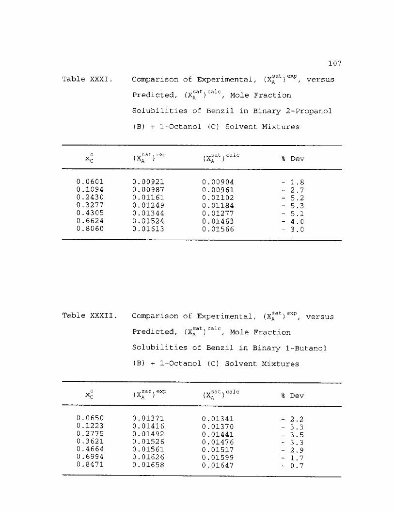
Table XXXI

107

Comparison of Experimental, (X sat N exp versus

Predicted, (X^at)calc, Mole Fraction

Solubilities of Benzil in Binary 2-Propanol

(B) + 1-Octanol (C) Solvent Mixtures

Xr . vsat, exp \ )

. vsat. calc % Dev

0.0601 0.1094 0.2430 0 .3277 0.4305 0.6624 0.8060

0.00921 0.00987 0.01161 0.01249 0.01344 0.01524 0.01613

0.00904 0.00961 0.01102 0.01184 0.01277 01463 01566

0 0

1 2 5 5 5 4 3

Table XXXII. Comparison of Experimental, (X^at)exp, versus

Predicted, (X^at)calc, Mole Fraction

Solubilities of Benzil in Binary 1-Butanol

(B) + 1-Octanol (C) Solvent Mixtures

. vsat N exp . vsat N calc ' A / % Dev

0.0650 0.1223 0.2775 0.3621 0.4664 0 .6994 0.8471

0.01371 0.01416 0.01492 0.01526 0.01561 0.01626 0.01658

0 .01341 0.01370 0.01441 0.01476 0.01517 0.01599 0.01647

2 3 3 3 2 1 0

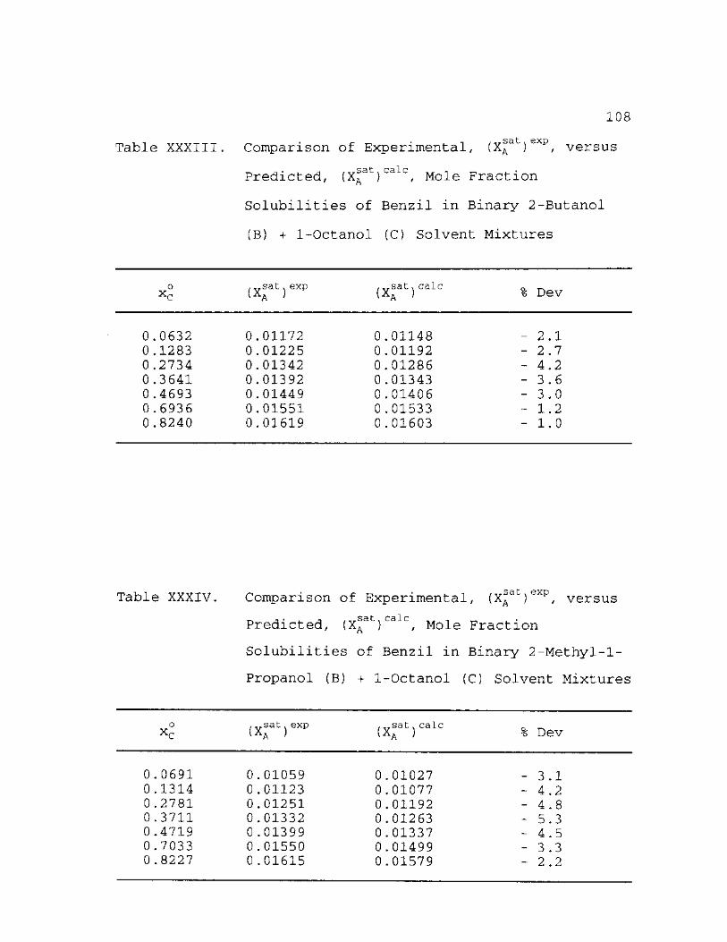
108

sat x exp versus Table XXXIII. Comparison of Experimental, (XA )

Predicted, (X*at)calc, Mole Fraction

Solubilities of Benzil in Binary 2-Butanol

(B) + 1-Octanol (C) Solvent Mixtures

=.t).xp , sat, calc ( ) % Dev

0.0632 0.1283 0.2734 0.3641 0.4693 0.6936 0.8240

0.01172 0.01225 0.01342 0.01392 0.01449 0.01551 0.01619

0.01148 0.01192 0.01286 0.01343 0.01406 01533 01603

0 0

2 2 4 3 3 1 1

Table XXXIV. Comparison of Experimental, (X^at)exp, versus

Predicted, (X^at)calc, Mole Fraction

Solubilities of Benzil in Binary 2-Methyl-l-

Propanol (B) + 1-Octanol (C) Solvent Mixtures

xr s a t) e X P (X sat. calc Dev

0.0691 0.1314 0 .2781 0.3711 0.4719 0.7033 0.8227

0.01059 0.01123 0.01251 0.01332 0.01399 0.01550 0.01615

0 0 01027 01077

0.01192 0.01263 0.01337 0.01499 0.01579

3 4 4 5 4 3 2

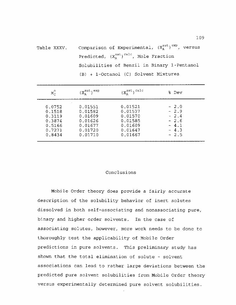
Table XXXV.

1 0 9

Comparison of Experimental, (X^at)exp, versus

Predicted, (X^at)calc, Mole Fraction

Solubilities of Benzil in Binary 1-Pentanol

(B) + 1-Octanol (C) Solvent Mixtures

o x c ( x * a t ) e x p , vsat.calc (XA ) % Dev

0 . 0 7 5 2 0 . 0 1 5 5 1 0 . 0 1 5 2 1 - 2 . 0

0 . 1 5 1 8 0 . 0 1 5 8 2 0 . 0 1 5 3 7 - 2 . 9

0 . 3 1 1 9 0 . 0 1 6 0 9 0 . 0 1 5 7 0 - 2 . 4

0 . 3 8 7 4 0 . 0 1 6 2 6 0 . 0 1 5 8 5 - 2 . 6

0 . 5 1 6 6 0 . 0 1 6 7 7 0 . 0 1 6 0 9 - 4 . 1

0 . 7 2 7 1 0 . 0 1 7 2 0 0 . 0 1 6 4 7 - 4 . 3

0 . 8 4 3 4 0 . 0 1 7 1 0 0 . 0 1 6 6 7 - 2 . 5

Conclusions

Mobile Order theory does provide a fairly accurate

description of the solubility behavior of inert solutes

dissolved in both self-associating and nonassociating pure,

binary and higher order solvents. In the case of

associating solutes, however, more work needs to be done to

thoroughly test the applicability of Mobile Order

predictions in pure solvents. This preliminary study has

shown that the total elimination of solute - solvent

associations can lead to rather large deviations between the

predicted pure solvent solubilities from Mobile Order theory

versus experimentally determined pure solvent solubilities.

110

In binary solvents, Mobile Order theory provides fairly

accurate predictions of solute solubility without adding

additional terms to specifically account for the increase in

solute - solvent hydrogen bonding that may occur as a result

of mixing two alcohol solvents.

Hydrogen bond strength depends on both the steric

hindrance around the hydrogen bonding sites as well as the

electron density around the electron donating site. A

comparison of Tables XIX - XXII reveals that the increased

steric hindrance surrounding the hydroxy proton of the

alcohol solvent significantly reduces the mole fraction

solubility of the solute by as much as 38 % in the three

branching alcohols studied. However, the steric hindrance

of the solvent seems to have less of an effect on the

solubility of thioxanthen-9-one, with an average reduction

in solubility of only 18 % for the three branching alcohol

solvents studied. This may be a result of solute - alcohol

complexes that are stronger for thioxanthen-9-one than

benzil.

In the case of compounds with sulfone functional

groups, the hydrogen bond between a hydroxy proton and a

sulfone oxygen should, in principle, be stronger than a

hydrogen bond between a hyroxy proton and alcohol oxygen

because the sulfone oxygen should have greater electron

density than the alcohol oxygen due to the electron donating

capabilities of sulfur's d-orbital through back-bonding.

Ill

But, on the other hand, the C-0 dipole moment is greater

than the S-0 dipole moment, so in this case the sulfone

oxygen should have less electron density than the alcohol

oxygen. From the data recorded, it appears that the

strength of the dipole moment has less of an effect on the

strength of the solute - solvent hydrogen bond than the

electron density of the electron donating site. When

comparing the magnitude of the solute - solvent association

constant of benzil to that of thioxanthen-9-one, one finds

that the association constant of thioxanthen-9-one is, on

average, 3.8 times larger than the association constant for

benzil if the benzil - 2-propanol constant is not

considered. This difference in the association constants

could be attributed to the steric hindrance surrounding the

lone pairs of electrons on the oxygen atom or to the

strength of the solute - solvent hydrogen bond, which

depends in part on steric hindrance.

One cannot completely attribute the enhancement in

solubility to the formation of solute - solvent

associations, nonspecific interactions in solution also play

a significant role in controlling the solubility of a

solute. Therefore, additional experimentation directly

comparing solutes with different functional groups capable

of donating electrons to a hydrogen bond should provide some

very interesting results, and hopefully shed some light on

the questions regarding hydrogen bond formation that have

112

yet to be resolved. At this point in time, it is unclear

whether a single averaged value adequately represents all

solute - solvent associations, or if individual averaged

values for each solute or solvent need to be determined.

Clearly additional research into the solution behavior of

PASHs is needed in order to discern a trend, if any, in the

solute - solvent association constant, which should improve

the pure solvent predictive capability of Mobile Order

theory.

113

Chapter References

1. Acree, W. E., Jr. Thermochim. Acta 1992 198, 71-79.

2. Acree, W. E., Jr.; Zvaigzne, A. I. Thermochim. Acta 1991 178, 151-167.

3. Acree, W. E., Jr.; McCargar, J. W.; Zvaigzne, A. I.; Teng, I.-L. Phys. Chem. Liq. 1991 23, 27-35.

4. Comer, J. F.; Kopecni, M. M. Anal. Chem. 1990 62, 991-994.

5. Acree, W. E., Jr.; Tucker, S. A. Phys. Chem. Liq. 1994 27, 1-9.

6. Weast, R. C. CRC Handbook of Chemistry and Physics 52nd

Edn.; CRC Press: Cleveland, OH, 1971.

7. Fletcher, K. A.; Pandey, S.; McHale, M. E. R.; Acree, W. E., Jr. J. Chem. Thermodyn., in press.

8. Acree, W. E., Jr.; Zvaigzne, A. I.; Tucker, S. A. Fluid Phase Equil. 1994 92, 233-253.

9. Ruelle, P.; Rey-Mermet, C.; Buchmann, M. ; Nairt-Tran, H.; Kesselring, U. W.; Huyskens, P. L. Pharm. Res. 1991 8, 840-850.

10. Ruelle, P.; Buchmann, M.; Nam-Tran, H.; Kesselring, U. w. Int. J. Pharm. 1992 87, 47-57.

11. Ruelle, P.; Sarraf, E.; Van den Berge, L.; Seghers, K.; Buchmann, M.; Kesselring, U. W. Pharm. Acta Helv. 1993 68, 49-60.

12. Huyskens, P. L.; Haulait-Pirson, M. C. J. Mol. Liq. 1985 31, 135-151.

13. Powell, J. R.; Voisinet, D.; Salazar, A.; Acree, W. E., Jr. Phys. Chem. Liq. 1994 28, 269-276.

14. Acree, W. E., Jr. Thermochim. Acta 1991 187, 37-56.

15. Sabbah, R.; El Watik, L Thermochim. Acta 1989 138, 241-247.

16. Sabbah, R.; El Watik, L. Can. J. Chem. 1992 70, 24-28.

114

17. Timmermans. J. Physico-Chemical Constants of Pure Organic Compounds; Elsevier: New York: NY, 1950.

18. Acree, W. E., Jr.; Tucker, S. A.; Zvaigzne, A. I. Phys. Chem. Lig. 1990 21, 45-49.

19. Huyskens, P. L.; Seigel, G. G. Bull. Soc. Chm. Belg. 1988 97, 821-824.

20. Acree, W. E., Jr.; Bertrand, G. L. J. Sol. Chem. 1983 12, 101-113.

21. Acree, W. E., Jr.; Rytting, J. H. J. Pharm. Sci. 1982 71, 201-205.

22. McHale, M. E. R; Kauppila, A.-S. M; Powell, J. R.; Acree, W. E., Jr. Phys. Chem. Lig. 1996 31, 175-181.

23. McHale, M. E. R; Kauppila, A.-S. M; Powell, J. R.; Otero, P., Jr.; Jayasakera, M.; Acree, W. E., Jr. J. Sol. Chem. 1996 25, 295-302.

24. Zvaigzne, A. I.; Powell, J. R.; Acree, W. E., Jr.; Campbell, S. W. Phys. Chem Lig. 1996 121, 1-13.

25. Acree, W. E., Jr.; Tucker, S. A. Fluid Phase Equil. 1994 102, 17-29.

26. Acree, W. E., Jr.; Zvaigzne, A. I. Fluid Phase Eguil. 1994 99, 167-183.

27. Acree, W. E.,Jr.; Tucker, S. A. Int. J. Pharm. 1994 101, 199-207.

28. Powell, J. R.; Fletcher, K. A.; Coym, K. S.; Acree, W. E., Jr.; Varanasi, V. G.; Campbell, S. W. J. Int. Thermophys., in press.

29. McHale, M. E. R.; Zvaigzne, A. I.; Powell, J. R.; Kauppila, A.-S. M.; Acree, W. E., Jr.; Campbell, S. W. Phys. Chem. Lig 1996 32, 67-85.

30. Powell, J. R.; McHale, M. E. R.; Kauppila, A.-S. M.; Acree, W. E., Jr.; Campbell, S. W. J. Soln. Chem. 1996 25, 1001-1017.

APPENDIX: GLOSSARY

Terms

activity thermodynamic function that aids in the mathematical description of a real system; defined as the ratio of the fugacity in a given state to the fugacity in a standard state

activity coefficient ratio of the activity of component i to its concentration; assigned a value of one for an ideal solution; represents a measure of the deviation of solution from ideality

amphiphilic solvents solvents that can function as both an electron donor and electron acceptor

associated solutions solution with molecular complexation

autoprotolysis self ionization of water where H+ and OH" ions are spontaneously formed in low concentration by the transfer of a proton from one water molecule to another

chemical potential change in the total free energy of the system at constant temperature and pressure when 1 mole of a given component is added to an infinite amount of the system, termed the partial molar Gibbs free energy of mixing

constant pressure heat capacity the energy required to raise the temperature of a body by 1°C at constant pressure.

dipole moment a measure of the distance between the centers of positive and negative charges on a polar molecule

domain average volume a molecule is assumed to occupy in solution

116

entropy of mixing the change in entropy that accompanies the mixing of two or more substances

ergodic the fraction of molecules involved in hydrogen bonding is equivalent to the fraction of time a given molecule is involved with a hydrogen bond with a neighboring molecule.

heat of fusion the change in enthalpy accompanying a change in state from a solid to a liquid

Henry's Law states, that for dilute solutions, the solubility of a solute is directly proportional to its partial pressure

heterogeneous associations in a binary mixture, associations between unlike molecules

homogeneous associations in a binary solvent mixture, the associations between molecules of the same species

hydrogen bond specific interaction that results from intermolecular attractions between a molecule containing and electron donor site and a molecule containing a proton donor site

ideal mole fraction solubility calculated as the activity of the solid solute when the activity coefficient is unity

ideal solution solution that shows no change in enthalpy or volume upon mixing and follows Raoult's law over all temperature and composition ranges

Kretschmer-Wiebe Associated Solution Model solution model that assumes the alcohol or amine forms continuous linear hydrogen bonded chains, and the stoichiometric volume fraction of the alcohol or amine is the sum of the volume fractions of each individual species

117

Mecke-Kempter Associated Solution Model solution model that assumes the self-associating species forms continuous linear hydrogen bonded chains with a single isodesmic equilibrium constant to describe the successive chemical reactions that build the chains

modified solubility parameter describes only the nonspecific interactions present in solution, all effects from specific interactions have been removed

molar volume volume of 1 mole of component i

mole fraction number of moles of component i divided by the number of moles present; solvent mole fractions are computed as if there was no solute present in solution

nonelectrolyte a substance that does not dissociate into ions when dissolved in solution

nonspecific interactions long range physical interactions in solution that result from weak dispersion forces

preferential solvation results whenever the solvent composition immediately surrounding the solute is different from the bulk solvent composition

Raoult's Law states that the fugacity of each component in a multicomponent mixture is equal to the product of the mole fraction composition of the specified component and the fugacity of the pure component at the temperature of the system. At low pressure fugacity is often replaced with vapor pressure.

specific interactions short range interactions between molecules in solution that result from specific, nonrandom contacts, i.e. hydrogen bonds

symmetrical reference state assumes the pure solid or liquid component at the temperature and pressure of the system as the standard state

118

triple point temperature temperature at which the solid, liquid and vapor phases are at equilibrium

unsymmetrical reference state distinguishes between the solvent and solute components; the solvent standard state is defined as a symmetrical reference state, the solute reference state is defined as a hypothetical infinite dilution standard state

volume fraction volume of component i divided by the total volume of all molecules present in solution

Symbols

measured absorbance of component i

Aij binary interaction parameter for describing physical, nonspecific molecular interactions between components i and j in the NIBS model for the physical contributions to the Gibbs free energy of mixing

aA°nd activity of the solid solute, defined as the ratio of the fugacity of the solid solute to the fugacity of the pure subcooled liquid

f solid, id . .

(aA ) ideal activity of solid solute, equivalent to the ideal mole fraction solubility

b length of sample cell through which radiation must pass in units of cm

Ci formal molar concentration of component i in . . 3 , - 1

units cm mol

ACp the constant pressure heat capacity of the solute

DomA average volume molecule A occupies in solution

119

AG chem

AG conf

A c r

^9mix

^ phys

AH fus

AH, fus TP

KA/ KB> KC

BC' - CB

K

N,

R

rc

AS

ROH

AS„

chemical contribution to the Gibbs free energy of mixing, depends upon the characteristics of the self-associating component(s)

configuration entropy contribution to the excess Gibbs free energy of mixing based upon the Huyskens and Haulait-Pirson definition of solution ideality

solute partial molar excess Gibbs free energy of mixing

Gibbs free energy of mixing

portion of the excess molar Gibbs free energy of mixing of the ij binary system which is attributes to nonspecific interactions, based upon the NIBS model

molar enthalpy of fusion of the solute at its normal melting point temperature

molar enthalpy of fusion of the solute at its triple point temperature

equilibrium constant for the formation of alcohol - alcohol homogeneous associations

equilibrium constant for the formation of alcohol - alcohol heterogeneous associations

equilibrium constant to describe solute -solvent associations

number of moles of component A in solution

number of alcohol molecules in a solution

gas constant, 8.3143 J K 1 mol 1

strucuration factor for solvent, assumed to be zero for nonassociating solvents, one for monofunctional alcohols, and two for water and diols

change in entropy upon the mixing of two or more components

temperature of the system in degrees Kelvin

120

Tmp normal melting point temperature at 1 atm of pressure

Ttp triple point temperature of the solute, temperature at which solid, liquid, and vapor phases are in equilibrium

V total molar volume of the solution in units cm mol

V° reduced volume of the domain of molecule A as a result of specific interactions in solution

VA, Vs molar volume of solute A and solvent S,

respectively in units of cm mol

Xi mole fraction composition of i

X>at saturation mole fraction solubility of the solute

(XAat)ld ideal mole fraction solubility of the solid

solute, equivalent to the activity of the solute when the activity coefficient is unity

Greek Letters

an fraction of alcohol molecules assumed to be involved in continuous hydrogen bond chain based on concentrations of alcohol molecules

?! weighting factor for component i used in the NIBS model for describing the physical contributions to the Gibbs free energy of mixing

Y the fraction of time an alcohol molecule is assumed to be free from hydrogen bonding

Yi activity coefficient of i

( Y r Vd ideal activity coefficient of solute, defined

as unity

YBh:'Ych: fraction of time one alcohol molecule, B or C, respectively, is free from hydrogen bonding

121

5A/5b,5c modified solubility parameter of solute,

solvent B, and solvent C, respectively

e molar absorptivity

r) refractive index

UA chemical potential of A

pA standard state chemical potential of A S 0. t <pA saturation volume fraction solubility of the

solute

S 9. t S 9. t

(4>a )b, (cf>A )c saturation volume fraction solubility of solute A in pure solvents B and C, respectively

REFERENCES

Acree, W. E., Jr. Current Topics in Sol. Chem. 1994 1-35.

Acree, W. E., Jr. Encyclopedia of Physical Science and Technology, Vol 11; Academic Press: Orlando, FL, 1992, 1-22 .

Acree, W. E., Jr. Thermochim. Acta 1991 187, 37-56.

Acree, W. E., Jr. Thermochim. Acta 1992 198, 71-79.

Acree, W. E., Jr. Thermodynamic Properties of Nonelectrolyte Solutions; Academic Press: Orlando, Fl, 1984; Chapter 2.

Acree, W. E., Jr. Thermodynamic Properties of Nonelectrolyte Solutions; Academic Press: Orlando, Fl, 1984; Chapter 3.

Acree, W. E., Jr. Thermodynamic Properties of Nonelectrolyte Solutions; Academic Press: Orlando, Fl, 1984; Chapter 5.

Acree, W. E., Jr. Thermodynamic Properties of Nonelectrolyte Solutions; Academic Press: Orlando, Fl, 1984; Chapter 10.

Acree, W. E., Jr.; Bertrand, G. L. J. Phys. Chem. 1977 81, 1170-1173.

Acree, W. E., Jr.; Bertrand, G. L. J. Sol. Chem. 1983 12, 101-113.

Acree, W. E., Jr.; McCargar, J. W. J. Mol. Liq. 1988 37, 251-261.

Acree, W. E., Jr.; McCargar, J. W.; Zvaigzne, A. I.; Teng, I.-L. Phys. Chem. Liq. 1991 23, 27-35.

Acree, W. E., Jr.; Rytting, J. H. J. Pharm. Sci. 1982 71, 201-205.

123

Acree, W. E., Jr.; Rytting, J. H. J. Pharm. Sci. 1983 72, 292-296.

Acree, W. E., Jr.; Tucker, S. A. Fluid Phase Equil. 1994 102, 17-29.

Acree, W. E., Jr.; Tucker, S. A. Int. J. Pharm. 1994 101, 199-207.

Acree, W. E., Jr.; Tucker, S. A. Phys. Chem. Liq. 1994 27, 1-9.

Acree, W. E., Jr.; Tucker, S. A.; Zvaigzne, A. I. Phys. Chem. Liq. 1990 21, 45-49.

Acree, W. E., Jr.; Zvaigzne, A. I. Fluid Phase Equil. 1994 99, 167-183.

Acree, W. E., Jr.; Zvaigzne, A. I. Thermochim. Acta 1991 178, 151-167.

Acree, W. E., Jr.; Zvaigzne, A. I.; Tucker, S. A. Fluid Phase Equil. 1994 92, 1-17.

Acree, W.E., Jr.; Zvaigzne, A.I.; Tucker, S.A. Fluid Phase Equil. 1994 92, 233-253.

Burchfield, T. E.; Bertrand, G. L. J. Sol. Chem. 1975 4, 205-214.

Comer, J. F.; Kopecni, M. M. Anal. Chem. 1990 62, 991-994.

Fletcher, K. A.; Coym, K. S.; Roy, L. E.; Hernandez, C. E.; McHale, M. E. R.; Acree, W. E., Jr. Phys. Chem. Liq., in press.

Fletcher, K. A.; McHale, M. E. R.; Coym, K. S.; Acree, W. E., Jr. Can. J. Chem. in press.

Fletcher, K. A.; McHale, M. E. R.; Powell, J. R.; Coym, K. S.; Acree, W. E., Jr. Phys. Chem. Liq., in press.

Fletcher, K. A.; Pandey, S.; McHale, M. E. R.; Acree, W. E., Jr. J. Chem. Thermodyn. in press.

Fletcher, K. A.; Pandey, S.; McHale, M. E. R.; Acree, W. E., Jr. Phys. Chem. Liq. 1996 33, 181-190.

Huyskens, P. L. J. Am. Chem. Soc. 1977 99, 2578-2582.

Huyskens, P. L. J. Mol. Struct. 1992 270, 197-203.

124

Huyskens, P. L. J. Mol. Struct. 1992 274, 223-246.

Huyskens, P. L. J. Mol. Struct. 1993 97, 141-147.

Huyskens, P. L.; Haulait-Pirson, M. C. J. Coat. Tech. 1985 57, 57-67.

Huyskens, P. L.; Haulait-Pirson, M. C. J. Mol. Lig. 1985 31, 135-151.

Huyskens, P. L.; Huyskens, D. P.; Siegel, G. G. J. Mol. Lig. 1995 64, 283-300.

Huyskens, P. L.; Haulait-Pirson, M. C.; Siegel, G. G.; Kapuku, F. J. Phys. Chem. 1988 92, 6481-6847.

Huyskens, P.; Kapuku, F.; Colemants-Vandevyvere, C. J. Mol. Struct. 1990 237, 207-220.

Huyskens, P. L.; Seghers, K. J. Mol. Struct. 1994 322, 75-82.

Huyskens, P. L.; Siegel, G. G. Bull. Soc. Chim. Belg. 1988 97, 821-824.

Huyskens, P. L.; Vael-Pauwels, C.; Seghers, K. Bull. Soc. Chim. Belg. 1992 101, 449-462.

Huyskens, P.; Van Beylen, M.; Verheyden, H. Pure and Appl. Chem. 1996 68, 1530-1540.

McCargar, J. W.; Acree, W. E., Jr. J. Soln. Chem. 1988 17, 1081-1091.

McHale, M. E. R.; Kauppila, A.-S. M.; Powell, J. R.; Acree, W. E., Jr. Phys. Chem. Lig. 1996 31, 175-182.

McHale, M. E. R.; Kauppila, A.-S. M.; Powell, J. R.; Otero, P., Jr.; Jayasekera, M.; Acree, W. E., Jr. J. Soln. Chem. 1996 25, 295-302.

McHale, M. E. R.; Pandey, S.; Acree, W. E., Jr. Phys. Chem. Lig., 1996 33, 93-112.

McHale, M. E. R.; Powell, J. R.; Kauppila, A.-S. M.; Acree, W. E., Jr.; Huyskens, P. L. J. Sol. Chem., in press.

McHale, M. E. R.; Zvaigzne, A. I.; Powell, J. R.; Kauppila, A.-S. M.; Acree, W. E., Jr.; Campbell, S.W. Phys. Chem. Lig. 1996 32, 67-85.

125

Nelis, K.; Van den Berge-Parmentier, L.; Huyskens, F. J. Mol. Lig. 1995 67, 157-174.

Pandey, S.; Powell, J. R.; McHale, M. E. R.; Kauppila, A.-S. M.; Acree, W. E., Jr. Fluid Phase Equil. 1996 123, 29-38.

Powell, J. R.; Acree, W. E., Jr.; Huyskens, P. L. J. Soln. Chem., in press.

Powell, J. R.; Fletcher, K. A.; Coym, K. S.; Acree, W. E., Jr.; Varanasi, V. G.; Campbell, S. W. submitted for publication in J. Int. Thermophys.

Powell, J. R.; McHale, M. E. R.; Kauppila, A.-S. M.; Acree, W. E., Jr.; Campbell, S. W. J. Sol. Chem. 1996 25, 1001-1017.

Powell, J. R.; McHale, M. E. R.; Kauppila, A.-S. M.; Otero, P.; Jayasekera, M.; Acree, W. E., Jr. J. Chem. Eng. Data 1992 40, 1270-1272.

Powell, J. R.; Voisinet, D.; Salazar, A.; Acree, W. E., Jr. Phys. Chem. Lig. 1994 28, 269-276.

Ruelle, P.; Buchmann, M.; Kesselring, U. W. J. Pharm. Sci. 1994 83, 369-403.

Ruelle, P.; Buchmann, M.; Nam-Tran, H.; Kesselring, U. W. Environ. Sci. Technol. 1993 27, 266-270.

Ruelle, P.; Buchmann, M.; Nam-Tran, H.; Kesselring, U. W. Int. J. Pharm. 1992 87, 47-57.

Ruelle, P.; Buchmann, M.; Nam-Tran, H.; Kesselring, U. W. J. Comp. Aid. Design 1992, 431-448.

Ruelle, P.; Buchmann, M.; Nam-Tran, H.; Kesselring, U. W. Pharm. Res,. 1992 9, 788-791.

Ruelle, P.; Kesselring, U. W. J. Mol. Lig. 1995 67, 81-94.

Ruelle, P.; Kesselring, U. W. J. Sol. Chem. 1996 25, 657-665.

Ruelle, P.; Kesselring, U. W. Pharm. Res. 1994 11, 201-205.

Ruelle, P.; Rey-Mermet, C.; Buchmann, M.; Nam-Tran, H.; Kesselring, U. W.; Huyskens, P. L. Pharm. Res. 1991 8, 840-850 .

126

Ruelle, P.; Sarraf, E.; Kesselring, U. W. Int. J. Pharm. 1994 104, 125-133.

Ruelle, P.; Sarraf, E.; Van den Berge, L.; Seghers, K.; Buchmann, M.; Kesselring, U. W. Pharm. Acta Helv. 1993 68, 49-60.

Sabbah, R.; El Watik, L. Can. J. Chem. 1992 70, 24-28.

Sabbah, R.; El Watik, L. Thermochim. Acta 1989 138, 241-247.

Seigel, G. G.; Huyskens, P. L.; Vanderheyden G. Ber. Bunsenges. Phys. Chem. 1990 94, 549-553.

Skoog, D. A.; Leary, J. J. Principles of Instrumental Analysis 4th ed. Philadelphia: Saunders College Publishing, 1992 Chapter 7.

Tinimermans. J. Physico-Chemical Constants of Pure Organic Compounds 1950 Elsevier, New York, New York.

Weast, R. C. CRC Handbook of Chemistry and Physics 52nd Edn. 1971 CRC Press, Cleveland, Ohio.

Zvaigzne, A. I.; Acree, W. E., Jr. J. Chem. Eng. Data 1995 40, 917-919.

Zvaigzne, A. I.; McHale, M. E. R.; Powell, J. R.; Kauppila, A.-S. M.; Acree, W. E., Jr., J. Chem. Eng. Data 1995 40, 1273-1275.

Zvaigzne, A. I.; Powell, J. R.; Acree, W. E., Jr.; Campbell, S. W. Phys. Chem Liq. 1996 121, 1-13.

Zvaigzne, A. I.; Teng, I.-L.; Martinez, E.; Trejo, J.; Acree, W. E., Jr. J. Chem. Eng. Data 1993 38, 389-392.