Embed Size (px)
Citation preview

Department of Mathematics and Statistics
Stability analysis of drinking epidemic models andinvestigation of optimal treatment strategy
Rinrada Thamchai
This thesis is presented for the Degree ofDoctor of Philosophy
ofCurtin University
December 2014

Declaration
To the best of my knowledge and belief, this thesis contains no material previously
published by any other person except where due acknowledgment has been made.
This thesis contains no material which has been accepted for the award of any
other degree or diploma in any university.
..........................................................
Rinrada Thamchai
December 2014
i

Abstract
In this research we first propose a more realistic drinking epidemic model, namely
the SPARS (susceptible-periodic-alcoholic-recovered drinkers) model. The ba-
sic reproduction number,R0, is then derived, and then we study the dynamical
behaviours of both drinking free equilibrium and drinking persistent equilibrium.
The purpose is to determine long term optimal treatment and short period pulsing
strategies for controlling the population of the periodic drinkers and alcoholics.
For long term optimal treatment, we show that an optimal control exists
which minimizes the number of periodic and hazardous drinkers (alcoholics). The
optimality is determined by using the Pontryagin Maximum Principle (PMP)
and the dynamic behaviour has been revealed through numerical simulations by
solving the underlying system of differential equations.
For short period pulsing strategy, we apply the pulse vaccination strategy
(PVS) in the SEIRS epidemic model to our SPARS drinking epidemic model.
Analytical results have been established for the stability of the periodic eradica-
tion solution and the persistent drinking for the SPARS model. The optimal
pulse treatment strategy has also been derived.
ii

List of publications during PhD
candidature
• R.Thamchai and Y.H. Wu. ”Stability Analysis and Optimal Treatmen-
t for the SPAR Drinking Epidemic Model”, Proceedings of International
Conference in Mathematics and Applications(ICMA - MU), 2011.
• R.Thamchai and Y.H. Wu. ”Stability Analysis and Optimal Treatment for
the SPAR Drinking Epidemic Model”, East-West Journal of Mathematics,
pp.347-360, a special volume 2012.
• R.Thamchai and Y.H. Wu. ”Impulsive Vaccination of SPARS Model with
Time Delays”, International Conference on Engineering and Applied Sci-
ence (ICEAS), ICEAS-1766, 2013.
iii

Acknowledgements
I wish to acknowledge the financial support of the Royal Thai Government Schol-
arship and Naresuan University for my PhD study.
I would like to express my thanks to my supervisor, Prof.Yong Hong Wu, for
his encouragement and supervision throughout the past three years with remark-
able patience and enthusiasm.
I would like to thank to my co-supervisor, Dr.Honglei Xu, for his advice and
encouragement during my PhD study.
I also wish to acknowledge the help from Prof.Benchawan Wiwatanapataphee
for her continuing encouragement and advice during my PhD study.
I would like to give thanks to all my friends and classmates for their assistances
and friendship particularly, Nathnarong Khajohnsaksumeth, Pawaton Kaemaw-
ithanurat, Wilaiporn Paisarn, Yaowanuch Raksong, Yan Zhang and Dr.Nattakorn
Phewchean.
I thank all of the staff in the Department of Mathematics and Statistics at
Curtin University for contributing to a friendly working environment. The ad-
ministrative staff, Joyce Yang, Shuie Liu, Lisa Holling, Jeannie Darmageo, Cheryl
Cheng and Carey Ryken Rapp, deserve special thanks for providing kind and pro-
fessional help on numerous occasions.
Finally, on a more personal note, I sincerely thank everyone in my family, es-
pecially my husband and my daughter, for their love, understanding and support
during my entire period of my PhD candidature in Australia.
iv

Contents
1 Introduction 1
1.1 Background . . . . . . . . . . . . . . . . . . . . . . . . . . . . . . 1
1.2 Objectives of the Thesis . . . . . . . . . . . . . . . . . . . . . . . 1
1.3 Outline of the Thesis . . . . . . . . . . . . . . . . . . . . . . . . . 2
2 Literature Review 4
2.1 Overview . . . . . . . . . . . . . . . . . . . . . . . . . . . . . . . . 4
2.2 Epidemic Model . . . . . . . . . . . . . . . . . . . . . . . . . . . . 4
2.2.1 Mathematical model . . . . . . . . . . . . . . . . . . . . . 4
2.2.2 SIR and SEIR Model . . . . . . . . . . . . . . . . . . . . 5
2.3 Optimal Control . . . . . . . . . . . . . . . . . . . . . . . . . . . 6
2.4 Impulsive Vaccination . . . . . . . . . . . . . . . . . . . . . . . . 9
2.4.1 Impulsive Differential Equations . . . . . . . . . . . . . . . 9
2.4.2 Comparison Theorem . . . . . . . . . . . . . . . . . . . . . 10
2.5 Previous Work on Drinking Epidemic . . . . . . . . . . . . . . . 12
2.6 Concluding Remarks . . . . . . . . . . . . . . . . . . . . . . . . . 17
3 Optimal Treatment for the Drinking Epidemic Model 19
3.1 General Overview . . . . . . . . . . . . . . . . . . . . . . . . . . . 19
3.2 Formulation and Analysis of the Drinking Epidemic Model . . . . 20
3.2.1 The SPARS Model . . . . . . . . . . . . . . . . . . . . . . 20
3.2.2 The Basic Reproduction Number . . . . . . . . . . . . . . 21
3.2.3 Stability of the equilibria . . . . . . . . . . . . . . . . . . . 22
3.3 Optimal Control . . . . . . . . . . . . . . . . . . . . . . . . . . . 24
3.4 Numerical Simulations . . . . . . . . . . . . . . . . . . . . . . . . 30
3.5 Concluding Remarks . . . . . . . . . . . . . . . . . . . . . . . . . 36
4 Drinking Epidemic Model with Time Delays and Impulsive Vac-
cination 37
4.1 General Overview . . . . . . . . . . . . . . . . . . . . . . . . . . . 37
4.2 Model Formulation and Lemmas . . . . . . . . . . . . . . . . . . . 38
v

4.3 Drinking-Free Periodic Solution . . . . . . . . . . . . . . . . . . . 40
4.4 Permanence of drinking . . . . . . . . . . . . . . . . . . . . . . . . 46
4.5 Numerical Simulations . . . . . . . . . . . . . . . . . . . . . . . . 49
4.6 Concluding Remarks . . . . . . . . . . . . . . . . . . . . . . . . . 60
5 Summary and Further Research 61
5.1 Summary . . . . . . . . . . . . . . . . . . . . . . . . . . . . . . . 61
5.2 Further Research . . . . . . . . . . . . . . . . . . . . . . . . . . . 62
Bibliography 63
vi
CHAPTER 1
Introduction
1.1 Background
Control of alcohol drinking is an important problem in many countries since al-
cohol plays a significant role in our society and our economy. Alcohol also has
dangerous effects on human body such as brain, heart, pancreas, liver and immune
system, as well as evaluating to other dangers such as loss of performance, absen-
teeism in the workplace, drink-driving and harm to others, anti-social behavior,
crime and family violence. Most drinkers try it for the first time as teenagers
or even in childhood. There are many reasons why people start drinking alco-
hol, including the curiosity, sociability, ignorance, imitation from their parents or
celebrities behavior. The explosion and spread of drinking has been studied for
many years. The prediction about drinking can help scientists to evaluate vacci-
nation or isolation plans and may have an important effect on the mortality rate
of drinking epidemic. Drinking epidemic model is a tool which has been used to
study the dynamic of the drinking spread, to predict the future and to simulate
the outbreak, as well as evaluating the strategies to control drinking epidemic.
1.2 Objectives of the Thesis
The aim of this project is to construct a robust drinking epidemic model, and
then study its dynamic properties and determine the optimal treatment strategy
to control the growth of periodic drinkers and alcoholics. The specific objectives
of this work are as follows.
(i) Establish a robust SPARS drinking epidemic model.As for the SEIRS
epidemic model, there is a significant period of time during which the in-
dividual has been infected but is not yet infectious themselves. We model
the drinking epidemic by considering the periodic drinkers (P ) to be the
1
1.3 Outline of the Thesis 2
individual latent period which is in compartment E (for exposed), and the
alcoholics (A) to be the infected (I).
(ii) Study the basic reproduction number, R0, and analyze the stability of the
equilibrium points of the SPARS model. The basic reproduction num-
ber concerns how many secondary drinkers resulted from the introduction
of an individual drinker into the population of susceptible. The value of
R0 indicates whether an epidemic is possible. Sensitivity analysis will be
performed on R0 and the stability of the system will also be examined.
(iii) Optimization is the strategy for controlling the number of individual drinker-
s. In our study, we will establish the optimal control problem of drinking
epidemic, and show the existence of an optimal control and then derive the
optimal system. The method used to determine the optimal strategy is the
Pontryagin Maximum Principle (PMP).
(iv) Investigate the properties of the model with pulse treatment. Since the
process of vaccination is discontinuous or repeated applications, it can be
described by impulsive differential equations. We call this kind of vacci-
nation strategies pulse vaccination strategy (PVS). We will consider pulse
treatment in the SPARS model, i.e. pulse vaccination strategy. We will
also study the pulse effects by analyzing the local and global stability of
equilibria.
1.3 Outline of the Thesis
In this thesis, various analytical and numerical results for the control of drinking
epidemic are developed. The thesis is organized into five chapters.
Chapter 1 gives an overview of the research background and the objectives of
the research.
Chapter 2 presents a literature review of the former work and results related
to this work including the review of fundamental equations and prior research
work in the field.
Chapter 3 presents the drinking epidemic model and analyze the basic re-
production number, R0, and the stability of equilibrium points. The Pontryagin

1.3 Outline of the Thesis 3
Maximum Principle (PMP) is used to determine the optimal system. The exis-
tence of an optimal control is established, followed by derivation of the optimal
system. Some numerical simulation results are also presented to demonstrate the
dynamics of the drinking epidemic model and to verify the analytical results.
Chapter 4 establishes the drinking epidemic model with time delays and im-
pulsive vaccination. The sufficient conditions are established for globally asymp-
totic stability of the drinking-free periodic solution and the permanence of the
model. Various numerical simulations are also presented to demonstrate the sys-
tem behaviour.
Chapter 5 summarizes the main results of this thesis and discusses further
research.

CHAPTER 2
Literature Review
2.1 Overview
Epidemiology is concerned with the distribution of diseases in populations and the
factors that influence the transmission of diseases. The epidemiologic approach
helps to explain the transmission of communication diseases, such as cholera and
measles [1]. Several epidemics models and associated theoretical studies are given
in Bailey [2], Anderson and May [3], Murray [4], Brauer and Castillo-Chavez
[5]. Although many social problems such as drug use [6, 7], zombie infection
[8], smoking [9] and alcohol drinking [10–13] have been referred to in terms of
epidemics, little has been published on the application of mathematical modeling
methods to such problems.
In this research we will investigate the dynamics of drinking epidemics and the
factors dominating the dynamics behave as well as the optimal control strategy.
This work will include construction of mathematical models, investigation of the
drinking epidemic treatment strategies, optimal control and the influences of
impulsive vaccination. Hence, in this chapter, we will first review topics relevant
to epidemic models in section 2.2. Then we will review the treatment strategies
and optimal control in section 2.3, followed by work in vaccination in section
2.4. Finally, the review of previous work and results in drinking epidemic are
represented in section 2.5 .
2.2 Epidemic Model
2.2.1 Mathematical model
A mathematical model is an interpreted or idealized illustration of a system or
process in mathematical terms, improvised to simplify calculation and prediction.
4
2.2 Epidemic Model 5
The efficiency of a model depends on the fact that it allows for the perception
and prediction of a phenomena without the work of performing the complex and
expensive experiments [14].
Mathematical modeling of infectious diseases is a tool which has been used
to study the mechanisms by which diseases spread, to predict the future course
of an outbreak. It can be used to study the effects of a variety of strategies for
disease eradication or control. A mathematical model for epidemics is in the
form of a system of equations subject to a set of initial and boundary conditions.
The structure and parameters involved in the equations are the main critical
elements of a mathematical model. Study of the properties of the model is also
as important as the model itself.
2.2.2 SIR and SEIR Model
Kermack and McKendrick developed the idea of threshold parameter in 1927, in-
vestigated and studied a basic SIR model [15]. In the model, all of the population
in community initially are susceptible to the disease and the infected individual
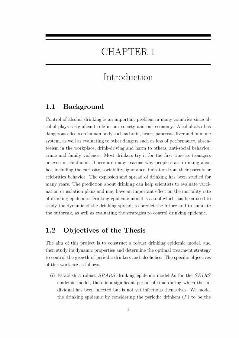
will have complete immunity after infection. The total population is divided into
three distinct categories: susceptible individuals (S), infected individuals (I) and
recovered individuals (R). The susceptible category is the healthy individuals
who may catch the disease. The infected category consists of members who have
the disease and may transmit it to others, and the recovered individuals are those
who were infected but have developed immunity to the infection. The change of
each of the individual categories is given in the flow chart below
Figure 2.1: Transfer diagram of the basic SIR model.
In the SIRS model, individuals recover with no immunity to the disease,
that is, individuals are immediately susceptible once they have recovered. The
dynamics of the SIR or SIRS have been widely analyzed [3, 5, 16].
There are many diseases for which individuals are not apparently infected
because it need a period of time for incubation. Therefore, the SIR and SIRS
models have been applied to studiy the transmission of diseases with a latent pe-
riod. By the assumption that before becoming infected individual, a susceptible

2.3 Optimal Control 6
Figure 2.2: Transfer diagram of the basic SIRS model.
individual may go through the latent period after catching the disease, the result-
ing models are of SEIR or SEIRS types, respectively, depending on whether
the recovered individual has the permanent immunity or not. Many studies have
been carried out for the SEIR and SEIRS model [17–19]. The state transfer
diagrams of the SEIR and SEIRS models are shown respectively in Figures 2.3
and 2.4.
Figure 2.3: Transfer diagram of the basic SEIR model.
Figure 2.4: Transfer diagram of the basic SEIRS model.
2.3 Optimal Control
Optimal control theory has found application in many fields, including economics,
finance, management, process control bioengineering and biological sciences. It
can be used to control an object to influence its behaviour so as to achieve a
desired goal with the constrains. In aerospace engineering, for example, optimal
control techniques can be applied to object correlation, fuel usage, spacecraft
2.3 Optimal Control 7
characterization etc. Another example is to determine the optimal percentage of
population which should be vaccinated to minimize the number of infected people
and the cost of vaccination.
Optimal control is a powerful method for solving dynamic optimization prob-
lems, when the problems are expressed in continuous time. The primary method
for optimal control was developed by Pontryagin et al. [20]. In this section,
we focus on review of optimal control theory of ordinary differential equations
(ODEs).
Lenhart and Workman [21] considered u(t) as the control and x(t) as the
state. The state variable is governed by a differential equation involving the
control variable:
x′(t) = g(t, x(t), u(t)). (2.1)
An optimal control problem consists of finding piecewise continuous control u(t)
and the associated state variable x(t) to maximize(minimize) the given objective
functional,
J(u) = maxu
(minu
)
∫ t1
t0
f(t, x(t), u(t))dt,
subject to x′(t) = g(t, x(t), u(t)),
x(t0) = x0 and x(t1) free.
(2.2)
Such a maximizing(minimizing) control is called an optimal control. By x(t1)
free, it means that the value of x(t1) is unrestricted; f and g are continuous dif-
ferentiable functions in all three arguments. Thus, the control(s) will always be
piecewise continuous and the associated states will always be piecewise differen-
tiable.
The principal technique for an optimal control problem is to solve a set of
”necessary conditions” that an optimal control and corresponding state must
satisfy. The necessary conditions are generated from the Hamiltonian H, which
is defined as follows;
H(t, x, u, λ) = f(t, x, u) + λg(t, x, u) (2.3)
Since, we want to maximize(minimize) H with respect to u at u∗, and the neces-

2.3 Optimal Control 8
sary conditions can be written in terms of the Hamiltonian:
∂H
∂uat u∗ ⇒ fu + λgu = 0 (optimality condition), (2.4)
λ′ = −∂H∂x⇒ −(fx + λgx) (adjoint equation), (2.5)
λ(t1) = 0 (transversality condition), (2.6)
where the dynamics of the state equation is
x′ = g(t, x, u) =∂H
∂λ, x(t0) = x0. (2.7)
Therefore, we can solve the optimal control problem by the following scheme;
(i) Form the Hamiltonian for the problem.
(ii) Set up the adjoint differential equations, transversality boundary conditions
and optimality conditions. Now there are three unknowns, u∗, x∗ and λ.
(iii) Eliminate u∗ by using the optimality equation Hu = 0, that is, solve u∗ in
terms of x∗ and λ.
(iv) Solve two differential equations for x∗ and λ with two boundary conditions,
substituting u∗ in the differential equations with the expression for the
optimal control from the previous step.
(v) After finding the optimal state and adjoint, solve the optimal control.
Application of control theory to epidemics is a very important field, and the
study of epidemic models is strongly related to the evaluation of different control
strategies: screening and educational campaigns [22], the vaccination campaign
[23], and resource allocation [24]. A comprehensive survey of control theory
applied to epidemiology was performed by Wickwire [25]. Many different models
with different objective functions have been proposed [9,26–29]. A major difficulty
in applying control methods to practical epidemiology problems is the commonly
made assumption that one has total knowledge of the state of the epidemics [30].
Zaman et al. [9] studied the stability of the equilibria for an SIR model.
In order to achieve control of the disease, they considered a control problem
associated with the SIR model. Some of the susceptible populations is vaccinated
in this model. They presented the existence of an optimal control for the control
problem and then conducted numerical simulations by using the Runge-Kutta

2.4 Impulsive Vaccination 9
fourth order procedure. Finally, they studied a real example to show the efficiency
of the optimal control.
Wiraningsih et al. [31] formulated a SEIR model for rabies between dogs and
human with vaccination effect. The basic reproduction number for this model is
derived, and the strategies for optimal distribution of vaccine to minimize the cost
of the control and the spread of the diseases is analyzed (minimize the infected
classes and maximize the susceptible classes). The optimality system is derived by
optimal control theory of the differential equation system and is then illustrated
by numerical results.
2.4 Impulsive Vaccination
The theory of impulsive differential equations has been extensively applied to
study evolution processes with a short term perturbation. Many processes and
phenomena in the real world exhibit impulsive effects particularly in mechanics,
control theory, pharmacokinetics, epidemiology, population dynamics, economics,
ecology [32–36].
2.4.1 Impulsive Differential Equations
Consider an evolution process [36] described by
(i) a system of differential equations
x′ = f(t, x), (2.8)
where f : R+ × Ω → Rn,Ω ∈ Rn is an open set and R+, the non-negative
real line;
(ii) the sets M(t), N(t) ∈ Ω for each t ∈ R+;
(iii) the operator A(t) : M(t)→ N(t) for each t ∈ R+.
Let x(t) = x(t, t0, x0) be any solution of (2.8) with initial value (t0, x0). The
process goes as follows: the point Pt = (t, x(t)) starts at the initial point Pt0 =
(t0, x0) and moves along the curve (t, x) : t ≥ t0, x = x(t) until t1 > t > 0, at
which the point Pt meets the set M(t). At t = t1, the operator A(t) transfers
the point to Pt+1 = (t1, x+1 ) ∈ N(t1), where x+
1 = A(t1)x(t1). Then the point
Pt continues its motion along the curve with x(t) = x(t, t1, x+1 ) as the solution
of (2.8) starting at Pt1 = (t1, x+1 ) until it hits the set M(t) again, at the next

2.4 Impulsive Vaccination 10
moment t2 > t1. Then, once again the point Pt2 = (t2, x(t2)) is transferred to
the point Pt+2 = (t2, x+2 ) ∈ N(t2), where x+
2 = A(t)x(t2). As before, the point Pt
continues to move forward with x(t) = x(t, t2, x+2 ) as the solution of (2.8) starting
at (t2, x+2 ). Thus the evolution process continues forward as long as the solution
of (2.8) exists.
We shall call the set of relations (i), (ii) and (iii), that characterize the above
mentioned evolution process, an impulsive differential system. The curve de-
scribed by the point Pt is called the integral curve, and the function x = x(t)
that defines this curve, a solution of the system.
Solutions of an impulsive differential system have the following three types:
(a) A continuous function, if the integral curve does not intersect the set M(t)
or hits it at fixed points of the operator A(t).
(b) A piecewise continuous function having a finite number of discontinuities of
the first kind if the integral curve meets M(t) at a finite number of points that
are not the fixed points of the operator A(t).
(c) A piecewise continuous function having a countable number of discontinuities
of the first kind if the integral curve encounters M(t) at a countable number of
points that are not the fixed points of the operator A(t).
2.4.2 Comparison Theorem
From [36], the theory of differential inequalities are essential in dynamics of dif-
ferential equations. The corresponding theory of impulsive inequalities is equally
useful in the investigation of impulsive differential equations.
To introduce the comparison principle of impulsive differential equations, we
firstly give the definition of extremal solutions of
u′(t) = g(t, u), t 6= τk,
u(t+k ) = ψ(u(tk)), t = τk,
u(t0) = u0,
(2.9)
where g ∈ C[R+ ×R,R] and ψk : R→ R.
Definition 2.1. [36] Let r(t) = r(t, t0, u0) be a solution of (2.9) on [t0, t0 + a).
A function r(t) is said to be the maximal solution of (2.9), if for any solution
u(t) = u(t, t0, u0) of (2.9) in [t0, t0 + a), the inequality
u(t) ≤ r(t), t ∈ [t0, t0 + a) (2.10)
2.4 Impulsive Vaccination 11
holds. A minimal solution ρ(t) may be defined similarly by reversing the (2.10).
Definition 2.2. [36] Let V : R+× rn → R+. V is said to belong to class V0 if V
satisfies:
(1) V is continuous on (tk−1, tk] × Rn and lim(t,y)→(t+k ,x) V (t, y) = V (t+k , x) for
every x ∈ Rn, k ∈ N ;
(2) V is locally Lipschitz continuous with respect to x.
Definition 2.3. [36] Let V ∈ V0, for (t, x) ∈ (tk−1, tk]×Rn. Define
D+V (t, x) = limh→0+
sup1
h[V (t+ h, x+ hf(t, x))− V (t, x)], (2.11)
and
D−V (t, x) = limh→0−
inf1
h[V (t+ h, x+ hf(t, x))− V (t, x)]. (2.12)
If the impulsive differential equation (2.9) and
dx
dt= f(t, x), t 6= τk,
∆x = Ik(x), t = τk,
x(t+0 ) = x0, t0 ≥ 0,
(2.13)
satisfy the conditions:
(1) 0 < t1 < t2 < ..., and tk →∞ as k →∞;
(2) f : R+ ×Rn → Rn is continuous on (tk−1, tk]×Rn and
lim(t,y)→(t+k ,x)
f(t, y) = f(t+k , x)
for every x ∈ Rn, k ∈ N ; (3) Ik : Rn → Rn;
(4) g : R+ ×R+ → R is continuous on (tk−1, tk]×Rn and
lim(t,y)→(t+k ,x)
g(t, y) = f(t+k , x)
for every x ∈ R+, k ∈ N ; then the following comparison principle holds.
Theorem2.4. [36] Let V : R+ × rn → R+, V ∈ V0. Suppose that
(1)g : R+ × R+ → R and satisfies the above conditions(4), and ψk : R → R is
nondecreasing and for each k = 1, 2, ...,
D+V (t, x) ≤ g(t, V (t, x)), t 6= τk,
V (t, x+ Ik(x)) ≤ ψk(V (t, x)), t = τk.(2.14)

2.5 Previous Work on Drinking Epidemic 12
(2) r(t) = r(t, t0, u0) is the maximal solution of (2.9) existing on [t0,∞). Then
V (t+0 , x0) ≤ u0 implies that
V (t, x(t)) ≤ r(t), t > t0,
where x(t) = x(t, t0, x0) is any solution of (2.13) on [t0,∞).
In recent years, pulse vaccination, repeated application of vaccine is gaining
prominence as a strategy for eliminating a variety of epidemics. Pulse vaccina-
tion strategy (PVS) consists of periodical repetitions of impulsive vaccinations
in population differently from the traditional constant continuous vaccination.
Many SIR and SEIR epidemic models with pulse vaccination were extensively
studied.
Zeng et al. [37] studied the impulsive control on an SIR epidemic model and
got the conditions on which epidemic-elimination solution is globally asymptoti-
cally stable and the conditions of bounded system. The differential susceptibility
SIR epidemic model with stage structure and pulse vaccination is introduced
by Zhang et al. [38]. Their work give some sufficient conditions for the globally
attractivity of an infection-free periodic solution and the permanence of infected
individual. Shi et al. [39] considered including the impulsive vaccination affects
on the original SIR system. Li and Yang [40] investigated two epidemic models
with continuous and impulsive vaccination strategies. The associated basic re-
production numbers were given and they compared the effect of control measures
on the spread of infection for the continuous and pulse vaccination strategies.
The application of PVS to SEIR models was discussed on d’Onofrio’s work
[41,42]. The author established the criteria for determining the space of vaccina-
tion parameters and the regions of local asymptotic stability (LAS). Furthermore,
the author studied analytically the global asymptotic stability (GAS) of the erad-
ication solutions in some cases and established the criterion which guarantees the
LAS of the eradication solutions.
2.5 Previous Work on Drinking Epidemic
The definition of alcoholism varies significantly between the medical community
and the treatment programs, such as Alcoholics Anonymous, which have been
set up to help alcoholics to recover. Even within the medical community there is
much debate about whether or not alcoholism should be considered as a disease. It
was only recently that epidemiology began to be applied to the study of this kind

2.5 Previous Work on Drinking Epidemic 13
of social problems. Since the beginning of this century, this area of mathematics
has started to become more prominent in the study of this type of problems and
other social phenomena, crime [43], drug abuse [6] and even the spread of urban
legends [44].
A simple SIR model for alcoholism is suggested by Sanchez et al. [10] in
which the population is divided into the following drinking classes: occasional
and moderate drinkers (S), problem drinkers (D), and temporarily recovered (R).
It is assumed that the population size remains constant, N . New recruits join
the population as occasional and moderate drinkers (S) and have homogeneous
mixing with the rest of the members of the population. A diagram of the various
rates affecting the three groups of individuals is represented in Figure 2.5 below.
Figure 2.5: Transfer diagram of Sanchez and his collaborators model.
The governing system of equations is
dS
dt= µN − βSD
N− µS,
dD
dt= β
SD
N+ ρ
RD
N− (µ+ φ)D,
dR
dt= φD − ρRD
N− µR,
S +D +R = N
(2.15)
The non - dimensionalized system of (2.15) is as follows:
s′ = µ− βsd− µs,
d′ = βsd+ ρrd− (µ+ φ)d,
r′ = φd− ρrd− µr,
s+ d+ r = 1
(2.16)
where s = SN, d = D
Nand r = R
N.

2.5 Previous Work on Drinking Epidemic 14
The parameters of this model are defined as follows:
µ : the birth and death rate.
β : the rate of recruitment to alcoholism due to encounters between occasional
and moderate drinkers and problem drinkers.
p : the rate at which recovered drinkers relapse to alcoholism.
φ : the rate of recovery.
The model’s basic reproduction number (R0), which gives the average number of
secondary drinker generated by the problem drinker in the population of moder-
ate drinkers, has been computed. For this model, the reproductive number with
recovery via treatment is R0 = βµ+φ
, where β is a measure of the influence of
problem drinkers on the susceptible individual and 1µ+φ
represents the average
time a problem drinker spends on the drinking class D [10].
Their results are not typical in epidemic models because the outcomes depend
not only on the value of R0 but on the size of the initial population of problem
drinkers. Especially, R0 < 1 does not guarantee the eradication of drinking
communities.
The results in this work also indicate that ineffective treatment programs
with high relapse rates may develop the spread of alcoholism, because they cre-
ate a group of recovered drinkers who could easily relapse. High relapse rates
will occur when treatment programs have only short-term positive effects. From
Witkiewitz’s research indicate that within the first year most of drinkers whose
receive treatment relapse to the lighter drinking [45]. An effective treatment s-
trategy for controlling the spread of alcoholism is to limit the amount of time a
recovered alcoholic spends in places where drinking occurs.
Benedict studied how alcoholism spreads, and how alcoholics relapse in [11].
At a standing-room-only talk at the 2006 Joint SMB - SIAM Conference on the
Life Sciences in Raleigh, North Carolina, Fabio Sanchez of Cornell University
presented a model for the spread of alcoholic drinking based on epidemiological
models of infectious diseases. By further developing Sanchez and his collabora-
tors’ model [10], the researcher investigate how the drinking problem spread by
alcoholics through social contacts among people with different drinking habits.
Newman [12] proposed the so-called SAR model which has similar parameters
and a similar SIR structure to the Sanchez model. However, it accounts for
not only recovered drinkers who relapse to occasional drinking but also those
recovered drinkers who relapse to problem drinking. Newman’s model also allows
the birth rate and death rates to take different values, and also includes a relapse
term from the recovered category to the susceptible class. Newman’s model was

2.5 Previous Work on Drinking Epidemic 15
further investigated by Benedict [11]. A diagram of the various rates affecting
the three groups of individuals is shown in Figure 2.6.
Figure 2.6: Transfer diagram of Newman model.
The Newman model can be described mathematically as follows:
dS
dt= µN − βSA
N+ εR− γS,
dA
dt= β
SA
N+ ρ
RA
N− φA− (γ + δ)A,
dR
dt= φA− ρRA
N− εR− (γ + δ)R,
S +D +R = N
(2.17)
where
µ is the birth rate;
β is the rate of recruitment to alcoholism due to encounters between suscep-
tible drinkers and alcoholics;
ε is the rate at which recovered drinkers relapse to moderate drinkers;
ρ is the rate at which recovered drinkers relapse to alcoholism;
φ is the rate of recovery;
γ is the natural death rate which is refer to any death rate not caused by
alcohol;
δ is the death rate related from drinking alcohol;
S is the number of susceptible drinkers;
A is the number of problem drinkers or alcoholics;
R is the number of temporarily recovered drinkers;
N is the number of total population.
This system (2.17) is subject to the following initial conditions
S(0) = S0 ≥ 0, A(0) = A0 ≥ 0, R(0) = R0 ≥ 0

2.5 Previous Work on Drinking Epidemic 16
where S0, A0 and R0 are constants. From (2.17), the total population N is defined
by the following equation
dN
dt= µN − δ(A+R)− γN (2.18)
Newman investigated the model and analyzed the basic reproduction number,R0,
which give the average number of people who will become alcoholism by intro-
ducing one alcoholic in the compartment.
Manthey et al. [13] analyzed the dynamics of campus drinking by using an
epidemiological model. They introduced a simple mathematical model capturing
the dynamics of the campus drinking phenomenon, which is focused on a college
campus and the student population is divided into three classes: non-drinkers
(N), social drinkers (S) and problem drinkers (P ). The student population is
assumed to be constant. The interactions between these three categories of stu-
dents are shown in Figure2.7.
As the work in [13] focuses on students in a college campus for a relatively
Figure 2.7: Transfer diagram of Manthey’s model.
short period of time only, their model does not include a recovered class and they
also regard students who stop drinking as non-drinkers. Therefore, their model
is a modified susceptible-infected-susceptible (SIS) model, and can be described
mathematically as follows:

2.6 Concluding Remarks 17
dN
dt= η − ηN − αNS − κNP + βS + εP,
dS
dt= σS − (η + σ)S + αNS − βS − γSP + δP,
dP
dt= πP − (η + π)P + γSP + κNP − δP − εP,
N + S + P = 1
(2.19)
where
α is the transmission rate of non-drinkers to social drinkers;
β is the recovery rate of social drinkers;
γ is the transmission rate of social drinkers to problem drinkers;
δ is the recovery rate of problem drinkers to social drinkers;
ε is the recovery rate of problem drinkers to non-drinkers;
η is the departure rate from campus environment;
π is the entrance rate of problem drinkers;
κ is the transmission rate of non-drinkers to problem drinkers;
σ is the number of problem drinkers or alcoholics;
R is the entrance rate of social drinkers;
N is the entrance rate of problem drinkers.
The model suggests that the reproductive number is not sufficient to predict
whether drinking behavior will persist on campus and that pattern of recruiting
new members plays a significant role in minimizing the campus alcohol problem.
2.6 Concluding Remarks
Various mathematical models for drinking epidemics have been developed. How-
ever, existing models still have some limitations and modification are required in
many aspects.
(i) The model presented by Sanchez assumes that the population is constant.
However in reality, this is not the case.
(ii) Sanchez’s model assumes that as people enter the population all of them
are occasional or social drinkers. In the real world, there are many people
who never try to have a drink.
(iii) Sanchez’s model assumes that an individual who enters the recovered drink-
ing group maintains immunity indefinitely. However, realistically, a recov-

2.6 Concluding Remarks 18
ered individual can relapse to the possible drinkers.
(iv) Normally, we can classified the drinkers in two categories; occasional drinker-
s and problem drinkers or alcoholics group like as Manthey’s model.
(v) Manthey’s model does not include a recovered class since they focus only
on students in a college campus for a short period of time (about 6 years
or less). To study the drinking epidemic not only in the college, one needs
to consider the recovered drinkers.
(vi) From the report [46], excessive alcohol use contributes to 88,000 deaths
in the United States each year, including 1 in 10 deaths among working
age adults. Excessive alcohol use includes binge drinking, heavy drinking.
Then, the death rate related to alcohol drinking in the alcoholics group
should not be equal to the death rate in other groups.
In this work, we will construct a more realistic drinking epidemic model and study
its behaviour and the method for the control of the behaviour.
CHAPTER 3
Optimal Treatment for the Drinking
Epidemic Model
3.1 General Overview
On the assumption that the spread of alcohol drinking follows a process similar
to that of disease transmission, mathematical epidemiological modeling of the
spread of alcohol drinking may give the conception on the evolution through the
drinking career, from initiation or occasional drinking to usual drinking, treat-
ment, relapse and final recovery. Benedict [11] described how alcoholism spreads,
and how alcoholics relapse by determining the effects of reproduction numbers on
the model dynamics and computing the equilibrium states of the model. Manthey
et al. [13] analyzed the dynamics of campus drinking by using an epidemiological
model. They introduced a basic drinking epidemic model to describe the dynam-
ics of the campus drinking behavior and their research focused on students at a
college campus. From their results, it can be concluded that the basic reproduc-
tion number is not sufficient to predict the behavior of drinking on this campus.
There is persistence of drinking that produced from the new initiate drinking
which is an interrupt to the reduction of the number of drinkers on the campus.
In this chapter, we develop a mathematical model for the control of alco-
hol drinking and then study its qualitative behavior. The rest of the chapter is
organized as follows. In section 3.2, the SPARS drinking epidemic model is estab-
lished, then an explicit expression for the basic reproduction number is derived,
and then the equilibrium points are determined and their stability are investigat-
ed. In section 3.3, an optimal control problem for finding the optimal treatment
(control) strategy is constructed, and then the Pontryagin Maximum Principle
(PMP) is used to find the optimal solution. In section 3.4, numerical examples
are given to validate the analytical results and to simulate the dynamic process
19

3.2 Formulation and Analysis of the Drinking Epidemic Model 20
of the movement of population among different groups. Finally, some conclusions
are given in section 3.5.
3.2 Formulation and Analysis of the Drinking
Epidemic Model
3.2.1 The SPARS Model
The model focuses on the population aged 16 and over. The population is divided
into four classes: susceptible drinkers (S), periodic drinkers (P ), alcoholics (A)
and recovered drinkers (R). The total population is denoted by N with N =
S + P +A+R. We assume that the recruitment rate is different from the death
rate which indicates that the total population is not constant. The interactions
between the four categories of population are shown in Figure 3.1.
Figure 3.1: Transfer diagram of the SPARS model.
The model presented in Figure 3.1 may be represented by the following system
of equations:
dS(t)
dt= µN(t)− αS(t)P (t)
N(t)− dS(t) + ηR(t),
dP (t)
dt= α
S(t)P (t)
N(t)− βP (t)− (d+ ε1)P (t),
dA(t)
dt= βP (t)− γA(t)− (d+ ε2)A(t),
dR(t)
dt= γA(t)− ηR(t)− (d+ ε3)R(t).
(3.1)
where
S(t) is the number of susceptible drinkers at time t,

3.2 Formulation and Analysis of the Drinking Epidemic Model 21
P (t) is the number of occasional or periodic drinkers at time t,
A(t) is the number of alcoholics or hazardous drinkers at time t,
R(t) is the number of temporality recovered drinkers at time t,
N(t) is size of the total population at time t,
µ is the rate of the general population entering the susceptible population,
that is, the demographic process of individuals reaching age 15 in the
modeling time period,
α is the contact rate between the susceptible and periodic drinkers,
β is the proportion of becoming an alcoholic,
γ is the proportion of hazardous drinkers who enter treatment,
η is the rate at which recovered drinkers relapse to susceptible drinkers,
d is the natural death rate of the general population,
ε1 is the death rate of occasional drinkers,
ε2 is the death rate of hazardous drinkers,
ε3 is the death rate of recovered drinkers.
We first find the equilibria of the SPARS model. By setting the RHS of the
system (3.1) to zero, we get two equilibrium states, namely the drinking free state
E0
(µNd, 0, 0, 0
)and the endemic state E1(K1N
α,ΛK2K3N,ΛβK3N,Λβγ),
where
K1 = (β + d+ ε1)
K2 = (γ + d+ ε2)
K3 = (η + d+ ε3)
Λ =(αµ−K1d)
α(K1K2K3 − βγη).
(3.2)
It is easy to see that K1K2K3 − βγη > 0, and therefore, the endemic state E1
occurs if and only if
αµ > K1d. (3.3)
3.2.2 The Basic Reproduction Number
The number of secondary drinkers produced by a single drinking individual in the
susceptible population is called the basic reproduction number,R0. The value of
R0 will indicates whether an epidemic is possible. Based on [47], the reproduction
number can be determined as the spectral radius of the next generation matrix.

3.2 Formulation and Analysis of the Drinking Epidemic Model 22
In the next generation matrix, the distinction between the drinkers and alcoholics
compartments must be determined from the epidemiological interpretation of the
model.
The drinking epidemic system (3.1) has a unique drinking free equilibrium
E0 (S0, 0, 0, 0) with S0 = µNd
. Taking the drinking compartments to be S and P
gives
[P ′
A′
]=
[αS0
N0
0 0
][P
A
]−
[β + d+ ε1 0
−β γ + d+ ε2
] P
A
=
[αµd
0
0 0
][P
A
]−
[K1 0
−β K2
][P
A
].
(3.4)
The next generation matrix can then be determined by K = FV −1 where
F =
[αµd
0
0 0
], V =
[K1 0
−β K2
].
Thus,
K = FV −1 =
[αµK1d
0
0 0
](3.5)
which has two eigenvalues λ = 0 , αµK1d
. Hence the basic reproduction number is
R0 = ρ(λ) =αµ
K1d. (3.6)
3.2.3 Stability of the equilibria
We now consider the stability of the two equilibrium states, namely the drinking
free equilibrium state E0 and the endemic state E1. For the system defined by
(3.1), the Jacobian matrix is the 4× 4 matrix given by
J =
−αPN− d −αS
N0 η
αPN
αSN−K1 0 0
0 β −K2 0
0 0 γ −K3
. (3.7)

3.2 Formulation and Analysis of the Drinking Epidemic Model 23
At the drinking free equilibrium E0
(µNd, 0, 0, 0
), the Jacobian matrix is
J0 = J
(µN
d, 0, 0, 0
)=
−d −αµ
d0 η
0 αµd−K1 0 0
0 β −K2 0
0 0 γ −K3
. (3.8)
By solving the characteristic equation det (J0 − λI) = 0, we obtain four eigenval-
uesλ1 = −d,
λ2 = −K2,
λ3 = −K3,
λ4 =αµ−K1d
d.
(3.9)
If R0 = αµK1d
< 1, i.e. αµ < K1d, then all the four eigenvalues are negative.
Therefore, we conclude that the drinking free equilibrium is locally asymptotical-
ly stable if R0 < 1, or unstable otherwise.
At the endemic state E1(K1Nα,ΛK2K3N,ΛβK3N,Λβγ), the Jacobian is
J1 = J(K1N
α,ΛK2K3N,ΛβK3N,Λβγ)
=
−αK2K3Λ− d −k1 0 η
αK2K3Λ 0 0 0
0 β −K2 0
0 0 γ −K3
.(3.10)
The characteristic equation of J1 is
λ4 + a1λ3 + a2λ
2 + a3λ+ a4 = 0 (3.11)
where
a1 = d+K2 +K3 + αK2K3Λ,
a2 = K2K3 + (αK2K3Λ + d) (K2 +K3) + αK1K2K3Λ,
a3 = K2K3 (d+ αΛ (K1K2 +K2K3 +K1K3)) ,
a4 = αK2K3Λ (K1K2K3 − ηβγ) .
(3.12)
3.3 Optimal Control 24
By the Routh-Hurwitz conditions [48], the equilibrium state is asymptotically
stable if
a1 > 0,
a3 > 0,
a4 > 0
a1a2a3 > a23 + a2
1a4.
(3.13)
From (3.2), we can see that K1 > 0, K2 > 0 and K3 > 0. Then, it is not difficult
to verify the validity of the above inequalities. Thus, for R0 > 1 there exists an
unique positive equilibrium E1 of the drinking epidemic model, which is always
locally asymptotically stable.
3.3 Optimal Control
For the optimal control problem, we let the control variables u1(t) be the edu-
cation campaign level used to control drinking in a community and u2(t) be the
level of treatment in the form of drinking.
The objective is to minimize the numbers of both occasional and hazardous
drinkers with minimum control. Hence, the optimal control problem can be
constructed as follows
OCP : J (u1, u2) =
T∫0
[δ1P (t) + δ2A(t) +
1
2
(ξ1u
21(t) + ξ2u
22(t))]dt,
(3.14)
subject to
dS(t)
dt= µN(t)− αS(t)P (t)
N(t)− dS(t) + ηR(t),
dP (t)
dt= α
S(t)P (t)
N(t)− (β + d+ ε1)P (t)− u1(t)P (t),
dA(t)
dt= βP (t)− (γ + d+ ε2)A(t)− u2(t)A(t),
dR(t)
dt= γA(t)− (η + d+ ε3)R(t) + u1(t)P (t) + u2(t)A(t),
(3.15)

3.3 Optimal Control 25
with initial conditions
S(0) = Ss , P (0) = Ps , A(0) = As , R(0) = Rs. (3.16)
Here δi and ξi for i = 1, 2 are weight factors (positive constants) representing
drinker’s level of acceptance of the control campaign. Let P (t) and A(t) be state
variables with control variables u1(t) and u2(t). Then we can rewrite the system
(3.15) in the following form:
φ′ = Bφ+ F (φ) := G(φ), (3.17)
where
φ =
S(t)
P (t)
A(t)
R(t)
,
B =
−d 0 0 η
0 − (β + d+ ε1 + u1(t)) 0 0
0 β − (γ + d+ ε2 + u2(t)) 0
0 u1(t) γ + u2(t) − (η + d+ ε3)
,
F (φ) =
µN − αSP
N
αSPN
0
0
.
Obviously (3.17) is a non-linear system with bounded coefficients. From the
non-linear term of the right hand side of (3.17), we have
F (φ1)− F (φ2) =
µN1 − αS1P1
N1
αS1P1
N1
0
0
−µN2 − αS2P2
N2
αS2P2
N2
0
0
(3.18)
3.3 Optimal Control 26
and thus
|F (φ1)− F (φ2)| =∣∣∣∣(µN1 − α
S1P1
N1
)−(µN2 − α
S2P2
N2
)∣∣∣∣+
∣∣∣∣αS1P1
N1
− αS2P2
N2
∣∣∣∣6 µ |N1 −N2|+
∣∣∣∣αS2P2
N2
− αS1P1
N1
∣∣∣∣+
∣∣∣∣αS1P1
N1
− αS2P2
N2
∣∣∣∣6 µ |N1 −N2|+ 2
∣∣∣∣αS1P1
N1
− αS2P2
N2
∣∣∣∣6 µ |N1 −N2|+ 2α
∣∣∣∣S1P1N2 − S2P2N1
N1N2
∣∣∣∣6 µ |N1 −N2|+ 2α |S1P1N2 − S2P2N1|
= µ |N1 −N2|+ 2α
∣∣∣∣(S1N2 + S2N1)
2(P1 − P2)
+(P2N2 + P1N1)
2(S1 − S2) +
(S2P2 + S1P1)
2(N2 −N1)
∣∣∣∣6 µ |N1 −N2|+ α |S1N2 + S2N1| |P1 − P2|
+α |P2N2 + P1N1| |S1 − S2|+ α |S2P2 + S1P1| |N2 −N1|
6M1 |S1 − S2|+M2 |P1 − P2|+M3 |N1 −N2| ,(3.19)
whereM1 = α |P2N2 + P1N1|
M2 = α |S1N2 + S2N1|
M3 = µ+ α |S2P2 + S1P1| .
Hence, we get
|G(φ1)−G(φ2)| 6 L |φ1 − φ2| (3.20)
where L = max M1,M2,M3, ‖B‖ <∞. Therefore, the function G is uniformly
Lipchitz continuous [49]. From the definitions of the control u1(t),u2(t) and the
control on S(t), P (t), A(t) and R(t), we can conclude that the solution of system
(3.20) exists [49], as described by the theorem below.
Theorem 3.1. Consider the optimal control problem OCP . There exists an
optimal control u∗ = (u∗1, u∗2) ∈ U such that
min(u1,u2)∈ U
J (u1, u2) = J (u∗1, u∗2) , (3.21)
with the state and control satisfying equations (3.15) and (3.16).

3.3 Optimal Control 27
Proof. For the existence of an optimal control, based on [50], the following con-
ditions must be satisfied.
(i) The set of controls and corresponding state variables are nonempty.
(ii) The control set U is convex and closed.
(iii) The RHS of the state system is bounded by a linear function in the state
and the control variables.
(iv) The integrand of the objective functional is concave on U .
(v) There exist constants c1, c2 > 0 and σ > 1 such that the integrand,
L(P,A, u1, u2), of the objective functional satisfies
L(P,A, u1, u2) ≥ c2 + c1
(|u1|2 + |u2|2
)σ2 . (3.22)
To verify all of these conditions, we use the result by Lukes [51] to give the
existence of solutions of the state system (3.15) with bounded coefficients, which
gives condition (i). The control set is closed and convex by definition, and thus
satisfies condition (ii). Since our state system is bilinear in u1 and u2 , the RHS of
the system (3.15) satisfies condition (iii), using the boundedness of the solutions.
In addition, the integrand of the objective functional (3.14) is convex on the
control set U . We can also easily see that there exist a constant σ > 1 and
c1, c2 > 0 since δ1, δ2, ξ1, ξ2 > 0, such that
δ1P (t) + δ2A(t) +1
2
(ξ1u
21(t) + ξ2u
22(t))≥ c2 + c1
(|u1|2 + |u2|2
)σ2 , (3.23)
which completes the proof for existence of the optimal control.
We can find an optimal solution of this optimal control problem by considering
the Lagrangian and the Hamiltonian for the problem. The Lagrangian of the
optimal control problem is given by
L (P,A, u1, u2) = δ1P (t) + δ2A(t) +1
2
(ξ1u
21(t) + ξ2u
22(t)). (3.24)
Applying Pontryagin’s Maximum Principle (PMP), we form the Hamiltonian and
derive the optimality system:
H (S, P,A,R, u1, u2, λ1, λ2, λ3, λ4)
= L (P,A, u1, u2) + λ1(t)dS(t)
dt+ λ2(t)
dP (t)
dt+ λ3(t)
dA(t)
dt+ λ4(t)
dR(t)
dt,
(3.25)
where λ1(t), λ2(t), λ3(t) and λ4(t) are the adjoint functions to be determined.

3.3 Optimal Control 28
Theorem 3.2. If (u∗1, u∗2) is an optimal pair with corresponding states S∗, P ∗, A∗
and R∗, then there exist adjoint variables λ1(t), λ2(t), λ3(t) and λ4(t), which sat-
isfy:
λ′1(t) =αP (t)
N(t)(λ1(t)− λ2(t)) + dλ1(t),
λ′2(t) = −δ1 +αS(t)
N(t)(λ1(t)− λ2(t))
+ (β + d+ ε1)λ2(t) + u1(t) (λ2(t)− λ4(t))− βλ3(t),
λ′3(t) = −δ2 + (γ + d+ ε2)λ3(t)− γλ4(t) + u2(t) (λ3(t)− λ4(t)) ,
λ′4(t) = −ηλ1(t) + (η + d+ ε3)λ4(t),
(3.26)
and the transversality conditions (boundary conditions) are
λi(tfinal = 0), i = 1, 2, 3, 4. (3.27)
Furthermore we obtain
u∗1(t) = max
min
(λ2(t)− λ4(t))
ξ1
P ∗(t) , ψ1
, 0
, (3.28)
u∗2(t) = max
min
(λ3(t)− λ4(t))
ξ2
A∗(t) , ψ2
, 0
. (3.29)
Proof. To consider the transversality conditions and the adjoint equations, the
method in [21] is used. From the Hamiltonian (3.25), we obtain (3.26) from
λ′1(t) = −∂H∂S
, λ′2(t) = −∂H∂P
, λ′3(t) = −∂H∂A
, λ′4(t) = −∂H∂R
. (3.30)
Using the optimal conditions and the property of the control space U for the
control variables u1 and u2 , we get
∂H
∂u1
= ξ1u1(t)− (λ2(t)− λ4(t))P ∗(t),
∂H
∂u2
= ξ2u2(t)− (λ3(t)− λ4(t))A∗(t).
(3.31)
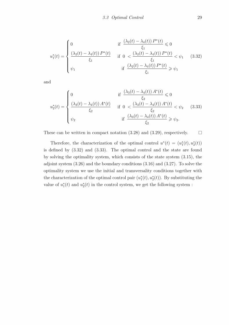
From the property of the control space, u∗1 and u∗2 are given by
3.3 Optimal Control 29
u∗1(t) =
0 if(λ2(t)− λ4(t))P ∗(t)
ξ1
6 0
(λ2(t)− λ4(t))P ∗(t)
ξ1
if 0 <(λ2(t)− λ4(t))P ∗(t)
ξ1
< ψ1
ψ1 if(λ2(t)− λ4(t))P ∗(t)
ξ1
> ψ1
(3.32)
and
u∗2(t) =
0 if(λ3(t)− λ4(t))A∗(t)
ξ2
6 0
(λ3(t)− λ4(t))A∗(t)
ξ2
if 0 <(λ3(t)− λ4(t))A∗(t)
ξ2
< ψ2
ψ2 if(λ3(t)− λ4(t))A∗(t)
ξ2
> ψ2.
(3.33)
These can be written in compact notation (3.28) and (3.29), respectively.
Therefore, the characterization of the optimal control u∗(t) = (u∗1(t), u∗2(t))
is defined by (3.32) and (3.33). The optimal control and the state are found
by solving the optimality system, which consists of the state system (3.15), the
adjoint system (3.26) and the boundary conditions (3.16) and (3.27). To solve the
optimality system we use the initial and transversality conditions together with
the characterization of the optimal control pair (u∗1(t), u∗2(t)). By substituting the
value of u∗1(t) and u∗2(t) in the control system, we get the following system :

3.4 Numerical Simulations 30
dS∗(t)
dt= µN(t)− αS
∗(t)P ∗(t)
N∗(t)− dS∗(t) + ηR∗(t),
dP ∗(t)
dt= α
S∗(t)P ∗(t)
N∗(t)
−[β + d+ ε1 −max
min
(λ2(t)− λ4(t))
ξ1
P ∗(t) , ψ1
, 0
]P ∗(t),
dA∗(t)
dt= βP ∗(t)
−[γ + d+ ε2 −max
min
(λ3(t)− λ4(t))
ξ2
A∗(t) , ψ2
, 0
]A∗(t),
dR∗(t)
dt=
[γ + max
min
(λ3(t)− λ4(t))
ξ2
A∗(t) , ψ2
, 0
]A∗(t)
−(η + d+ ε3)R∗(t)
+ max
min
(λ2(t)− λ4(t))
ξ1
P ∗(t) , ψ1
, 0
P ∗(t),
(3.34)
with the Hamiltonian,
H∗ (S∗, P ∗, A∗, R∗, u∗1, u∗2, λ1, λ2, λ3, λ4)
= δ1P∗(t) + δ2A
∗(t) +1
2
[ξ1
(max
min
(λ2(t)− λ4(t))
ξ1
P ∗(t), ψ1
, 0
)2
+ ξ2
(max
min
(λ3(t)− λ4(t))
ξ2
P ∗(t), ψ2
, 0
)2]
+λ1(t)dS∗(t)
dt+ λ2(t)
dP ∗(t)
dt+ λ3(t)
dA∗(t)
dt+ λ4(t)
dR∗(t)
dt.
(3.35)
The optimal control and the corresponding states have been determined. Next
we will show the numerical simulation that solve system (3.34) and Hamiltonian
(3.35).
3.4 Numerical Simulations
A number of numerical simulations were carried out using MATLAB to illustrate
the dynamics of the system. The parameter values used in the numerical simu-
lations are : µ = 0.085, α = 0.02, β = 0.01, γ = 0.001, d = 0.075, η = 0.001, ε1 =
0.001, ε2 = 0.01 and ε3 = 0.002. The percentages of initial individuals in suscep-
tible, periodic, alcoholics and recovered classes are 50, 30, 15 and 5, respectively.
The evolution of each class of population with time is shown in Figure 3.2. The

3.4 Numerical Simulations 31
results show that the drinking free state of the system is asymptotically stable,
which is as expected from our analysis as R0 = αµ(β+d+ε1) d
= 0.26 < 1. Moreover,
we considered another case in which the contact rate between the susceptible and
periodic drinkers is α = 0.2 which is given R0 > 1. The evolution of each class
of population in this case is shown in Figure 3.3. Obviously, the asymptotically
stable endemic state has been captured in this case.
The optimal control problem for the SPARS model is solved numerically. We
used an iterative method such as the Runge-Kutta fourth order scheme to solve
this optimality system by using the method in [21]. The state variables S, P,A
and R are solved forward in time by using an initial guess of the control variables
u1(t) and u2(t). Conversely, the adjoint variables, λi for i = 1, 2, 3, 4 are solved
backwards in time. For the SPARS model presented in this work, the state
system is given by (3.15). The adjoint system is given by (3.26) with the final
time conditions given by (3.27) and the characterization of the optimal control
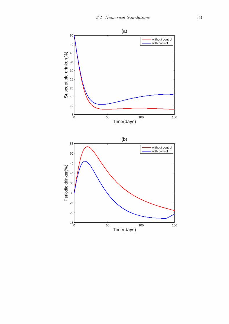
by (3.28) and (3.29). The numerical results obtained are presented in Figure 3.4.
In Figure 3.4(a) and 3.4(e), we see that the number of susceptible drinkers
and the total population, respectively, with control are greater than those with-
out control, which can be caused by the education control that we put on the
susceptible individual and the treatment control on the recovered drinkers for
which this group could be relapse to susceptible group.
In Figure 3.4(b) and 3.4(c), we have plotted the periodic drinkers and alco-
holics, respectively, with and without control. We see that in the first ten to
fifteen days the number of population with and without control in both cate-
gories does not differ very much; but as time increases, the difference becomes
substantial.
In Figure 3.4(d), the comparison of education control ,u∗1, and the treatment
control ,u∗2, are plotted as a function of time in days.

3.4 Numerical Simulations 32
0 100 200 300 400 5000
10
20
30
40
50
60
70
80
90
100
Time(days)
Indi
vidu
als
in e
ach
clas
s(%
)
SPAR
Figure 3.2: The evolutions of the four classes of populations when R0 < 1.
0 100 200 300 400 5000
10
20
30
40
50
60
70
Time(days)
Indi
vidu
als
in e
ach
clas
s(%
)
SPAR
Figure 3.3: The evolutions of the four classes of populations when R0 > 1.
3.4 Numerical Simulations 33
0 50 100 1505
10
15
20
25
30
35
40
45
50
Time(days)
Sus
cept
ible
drin
ker(
%)
(a)
without controlwith control
0 50 100 15015
20
25
30
35
40
45
50
55
Time(days)
Per
iodi
c dr
inke
r(%
)
(b)
without controlwith control

3.4 Numerical Simulations 34
0 50 100 15010
15
20
25
30
35
40
Time(days)
Alc
ohol
ic(%
)
(c)
without controlwith control
0 50 100 1500
5
10
15
20
25
30
35
40
Time(days)
Rec
over
ed d
rinke
r(%
)
(d)
without controlwith control

3.4 Numerical Simulations 35
0 50 100 15060
65
70
75
80
85
90
95
100
Time(days)
Tot
al P
opul
atio
n(%
)
(e)
without controlwith control
135 135.5 136 136.5 137 137.5 138−0.01
−0.005
0
0.005
0.01
0.015
0.02
Time(days)
Con
trol
Rat
e
(f)
Educational control(u1* )
Treatment control(u2* )
Figure 3.4: Diagrams showing the effects of drinking control on the evolutions
of the four classes of populations : (a) susceptible drinker; (b) periodic drinker;
(c) alcoholic; (d) recovered drinker; (e) total population; (f) the optimal controls
u∗1(t) and u∗2(t).
3.5 Concluding Remarks 36
3.5 Concluding Remarks
An SPARS model has been proposed to describe the overall drinking population
dynamics for the case in which the total population is not constant and the death
rates for different population groups are different. The model is constructed
taking into account the periodic drinkers compartment with bilinear incidence
rate. Analysis of the model shows that there are two equilibria, drinking free state
and endemic state. An explicit expression for the basic reproduction number,
R0, has been derived and it has been shown that when R0 < 1, that is α <(β+d+ε1) d
µ, the drinking free equilibrium is locally asymptotically stable. The
drinking endemic state has also been shown to be locally asymptotically stable
for R0 > 1. An optimal control problem has also been constructed to determine
the optimal treatment strategies to minimize the number of drinkers and the
resources for the control. The results show that the number of periodic drinkers
and alcoholics decreases significantly in the optimal controlled system. It is found
that the numerical results agree with the analytical results derived.

CHAPTER 4
Drinking Epidemic Model with Time
Delays and Impulsive Vaccination
4.1 General Overview
The common method used for controlling the epidemic disease is vaccination. We
normally adopt the vaccination to control or eradicate the spread. Vaccinations
have many types. Constant vaccination and pulse vaccination are two main s-
trategies [52]. Constant vaccination is a primary vaccination strategy that can
protect the individual who received the vaccine. But this method of vaccination
is not always sufficient for disease eradication and does not offer 100% protection,
and some of individual get infected despite of vaccination [53]. Pulse vaccination
strategy (PVS) is a method used to eliminate an epidemic disease by injection or
vaccination repeated on a risk group over a defined age range [41,54]. Even though
the effect of continuous vaccination strategy is better than impulsive vaccination
strategy, the side effect of the cost and the material have potential harmful ef-
fects, especially for infants. So we prefer to the impulsive vaccination strategy as
it is easier to be manipulated and it has the relatively low cost [52,55–57].
The scientists at the University of Chile developed an experimental drug to
cure alcoholism. If a person who has received the vaccine try to drink alcohol, they
will almost immediately get severe nausea, accelerated heartbeat and discomfort,
according to the Daily Mail [58]. The shot is effective for about six months to a
year and works by speeding up the hangover process.
In recent years, many epidemic models with time delay were largely studied
in [59–63]. Some of the research literature on SEIR or SEIRS epidemic models
are established by ODEs [17, 64–67]. Impulsive differential equations and time
delay are introduced to describe the dynamics of epidemic disease [68–75], and
most of these research literature are on SEIRS model.
37

4.2 Model Formulation and Lemmas 38
Meng et al. [76] proposed and analyzed the dynamic behaviors of an SEIRS
epidemic model with pulse vaccination and two time delays under the condition
of nonlinear incidence rate. Using the stroboscopic map, the authors determined
the dynamics of the discrete system and presented the existence of an infection-
free periodic solution. Whenever the period of impulsive effect is less than some
critical value, the stability of the infection-free equilibrium is globally attractive.
Moreover, they obtained the efficient conditions for the persistence of epidemic
model with pulse vaccination.
An impulsive vaccination of the SEIR epidemic model with two time delays is
formulated by Gao and his teamwork [77]. They obtained the infection-free peri-
odic solution of the system. Moreover, they found that whenever the vaccination
rate is greater than θ∗ ,the infected disease dies out, while if the vaccination rate
is less than θ∗, the disease will be permanence.
In this chapter, an SPARS drinking epidemic model with two time delays
and impulsive vaccination is investigated in section 4.2 including some lemmas
that we will use for considering the stability of periodic solution. In section 4.3,
the property of periodic solution is investigated, while the essential conditions
for the permanence of the drinking is obtained in section 4.4. In section 4.5,
numerical examples are given to validate the analytical results and to simulate the
dynamic process of the movement of population among different groups, followed
by concluding remarks in section 4.6.
4.2 Model Formulation and Lemmas
In this study, we set the SPARS drinking epidemic model with two time delays
and impulsive vaccination by the following assumptions:
(i) The total population(N) is partitioned into four classes, the susceptible
drinkers(S), periodic drinkers(P ), alcoholics(A) and recovered drinkers(R).
(ii) The natural death rate is assumed to be the same positive constant d for
all four categories, and the extra death rates taking into account the effect
of drinking in the categories of periodic, alcoholic and recovered drinker are
ε1, ε2 and ε3, respectively. We also assume that the influx of susceptible
population from a constant recruitment is K.
(iii) The contact rate α is defined as the expected number of contacts at which
potentially drinking occurs between susceptible individual and others. The
rate at which an occasional drinker becomes an alcoholic is β with the addict

4.2 Model Formulation and Lemmas 39
period ω; the alcoholics receive treatment with rate γ and the recovered
drinkers relapse to susceptible drinkers with rate η in the period τ .
(iv) The proportion of successful vaccination, which is called pulse vaccination
rate, is θ (0 < θ < 1), and the interpulse time or the time between two
consecutive pulse vaccinations is T .
The SPARS drinking epidemic model with two time delays and impulsive
vaccination is established as follows
S ′(t) = K − αS(t)P (t)
N(t)− dS(t) + ηR(t− τ)e−(d+ε3)τ
P ′(t) = αS(t)P (t)
N(t)− βP (t− ω)e−(d+ε1)ω − (d+ ε1)P (t)
A′(t) = βP (t− ω)e−(d+ε1)ω − γA(t)− (d+ ε2)A(t)
R′(t) = γA(t)− ηR(t− τ)e−(d+ε3)τ − (d+ ε3)R(t)
t 6= kT, k ∈ N
S(t+) = (1− θ)S(t)
P (t+) = P (t)
A(t+) = A(t)
R(t+) = R(t) + θS(t)
t = kT, k ∈ N
(4.1)
Note that in model (4.1), we consider the impulsive vaccination of the SPARS
model with time delays and the influx of susceptible comes from the constant
recruitment rate, K, which is different to the original SPARS model in (3.1)
on which the population enter the susceptible population from the demographic
process of individuals reaching age 15 in the modeling time period.
The total population size N(t) can be determined by
N ′(t) = K − dN(t)− (ε1P (t) + ε2A(t) + ε3R(t))
N(t+) = N(t)(4.2)
Thus, the total population size may vary in time. From (4.2), we have
K − (d+ ε1 + ε2 + ε3)N(t) 6 N ′(t) 6 K − dN(t) (4.3)
It follows that
K
d+ ε1 + ε2 + ε3
6 limt→∞
inf N(t) 6 limt→∞
supN(t) 6K
d(4.4)

4.3 Drinking-Free Periodic Solution 40
In the following, some previous results which are to be used in establishing
our main results, are given.
Lemma 4.1. [73] Consider the following equation:
x′(t) = a1x(t− ω)− a2x(t) (4.5)
where a1, a2, ω > 0 for −ω 6 t 6 0. We have
(i) If a1 < a2 , then limt→∞
x(t) = 0
(ii) If a1 > a2 , then limt→∞
x(t) =∞The proofs of case (i) and (ii) are given in Theorem 3.2.1 [78] and Lemma 2.1
[79],respectively.
Lemma 4.2. [73] Consider the following impulsive differential equation
u′(t) = a− bu(t), t 6= kT, k ∈ Nu(t+) = (1− θ)u(t), t = kT, k ∈ N
(4.6)
where a > 0, b > 0 and 0 < θ ≤ 1. Then, there exists a unique periodic solution
of system(4.6):
u(t) =a
b+(u∗ − a
b
)e−b(t−kT ), kT < t ≤ (k + 1)T (4.7)
which is globally asymptotically stable, where u∗ = a(1−θ)(1−e−bT )
b(1−(1−θ)e−bT ).
Lemma 4.3. [80] Consider the following impulsive differential equation
u′(t) = a− bu(t)− cu(t− T ), t 6= kT, k ∈ Nu(t+) = (1− θ)u(t), t = kT, k ∈ N
(4.8)
where a > 0, b > 0, c > 0 and 0 < θ ≤ 1.Then there exists a unique periodic
solution of system (4.8) which is globally asymptotically stable.
4.3 Drinking-Free Periodic Solution
Since A(t) = N(t) − (S(t) + P (t) +R(t)), we focus on the following equivalent
model of (4.1);

4.3 Drinking-Free Periodic Solution 41
S ′(t) = K − αS(t)P (t)
N(t)− dS(t) + ηR(t− τ)e−(d+ε3)τ
P ′(t) = αS(t)P (t)
N(t)− βP (t− ω)e−(d+ε1)ω − (d+ ε1)P (t)
R′(t) = γN(t)− γS(t)− γP (t)− ηR(t− τ)e−(d+ε3)τ
−(γ + d+ ε3)R(t)
N ′(t) = K − (d+ ε2)N(t) + ε2S(t) + (ε2 − ε1)P (t)
+(ε2 − ε3)R(t)
t 6= kT, k ∈ N
S(t+) = (1− θ)S(t)
P (t+) = P (t)
R(t+) = R(t) + θS(t)
N(t+) = N(t)
t = kT, k ∈ N
(4.9)
In this section, we first analyse the system (4.9) by demonstrating the exis-
tence of a drinking-free periodic solution, in which periodic drinking individuals
are permanently absent from the population, i.e. P (t) = 0 for all t > 0. Un-
der this condition the dynamics of susceptible individuals, alcoholics, recovered
individuals and total population must satisfy the following system :
S ′(t) = K − dS(t) + ηR(t− τ)e−(d+ε3)τ
R′(t) = γN(t)− γS(t)− ηR(t− τ)e−(d+ε3)τ − (γ + d+ ε3)R(t)
N ′(t) = K − (d+ ε2)N(t) + ε2S(t) + (ε2 − ε3)R(t)
t 6= kT, k ∈ N
S(t+) = (1− θ)S(t)
R(t+) = R(t) + θS(t)
N(t+) = N(t)
t = kT, k ∈ N
(4.10)
Since limt→∞
N(t) > Kd+ε2
and Kd+ε1+ε2+ε3
6 limt→∞
inf N(t) 6 limt→∞
supN(t) 6 Kd
,
we can say that limt→∞
N(t) 6 Kd
. If P (t) ≡ 0, it follows from the third and seventh
equations of model(4.1) that limt→∞
A(t) = 0. Therefore we have the following limit
system of (4.10)
R(t) =K
d− S(t) (4.11)

4.3 Drinking-Free Periodic Solution 42
and
S ′(t) = K
(1 +
ηe−(d+ε3)τ
d
)− dS(t)− ηe−(d+ε3)τS(t− τ), t 6= kT
S(t+) = (1− θ)S(t), t = kT
(4.12)
According to Lemma 4.2, we can see that if d > ηe−(d+ε3)τ , then the system
(4.12) has a unique positive periodic solution with period T which is globally
asymptotically stable. We denote this periodic solution by S(t). Therefore, the
drinking-free periodic solution of system (4.10) is(S(t), 0, K
d− S(t), K
d
).
From the delayed SPARS drinking epidemic model (4.1), letting the drinking
compartments to be P and A gives[P ′
A′
]=
[αS∗
N∗ 0
0 0
][P
A
]−
[d+ ε1 + βe−(d+ε1)ω 0
−βe−(d+ε1)ω γ + d+ ε2
][P
A
](4.13)
The next generation matrix can then be determined by L = FV −1 where
F =
[αS∗
N∗ 0
0 0
], V =
[d+ ε1 + βe−(d+ε1)ω 0
−βe−(d+ε1)ω γ + d+ ε2
].
Thus,
L = FV −1 =
[αS∗
(d+ε1+βe−(d+ε1)ω)N∗ 0
0 0
](4.14)
which has two eigenvalues;
λ = 0 ,αS∗
(d+ ε1 + βe−(d+ε1)ω)N∗,
where S∗ = K(d+ηe−(d+ε3)τ )(1−e−dT )d2(1−(1−θ)e−dT )
and N∗ = Kd
.
Hence the basic reproduction number is
R∗ =α(d+ ηe−(d+ε3)τ )(1− e−dT )
d(d+ ε1 + βe−(d+ε1)ω)(1− (1− θ)e−dT ).(4.15)

4.3 Drinking-Free Periodic Solution 43
Theorem 4.4. If R∗ < 1, the drinking-free periodic solution (DFPS)(S(t), 0, K
d− S(t), K
d
)is globally attractive, where
R∗ =α(d+ ηe−(d+ε3)τ )(1− e−dT )
d(d+ ε1 + βe−(d+ε1)ω)(1− (1− θ)e−dT )(4.16)
Proof. SinceR∗ < 1, we can choose ε0 > 0 small enough such that
αdΓ
K< (d+ ε1 + βe−(d+ε1)ω) (4.17)
where Γ = K(d+ηe−(d+ε3)τ )(1−e−dT )d2(1−(1−θ)e−dT )
+ ε0.
From system(4.12), we consider the following comparison impulsive differen-
tial system :
X ′(t) = K
(1 +
ηe−(d+ε3)τ
d
)− dX(t), t 6= kT, k ∈ N
X(t+) = (1− θ)X(t), t = kT, k ∈ N.
(4.18)
By Lemma 4.2, we have a periodic solution of system (4.18) as follows
X(t) = ξ + (X∗ − ξ)e−d(t−kτ) , kT < t 6 (k + 1)T (4.19)
which is globally asymptotically stable, where ξ = K d+ηe−(d+ε3)τ
d2and
X∗ = ξ(1−θ)(1−e−dT )(1−(1−θ)e−dT )
for k > k1.
Therfore,
S(t) < X(t) 6 X(t) + ε0 6K(d+ ηe−(d+ε3)τ )(1− e−dT )
d2(1− (1− θ)e−dT )+ ε0 , Γ (4.20)
Further, from the second equation of system (4.27), we have
P ′(t) = αS(t)P (t)
N(t)− βP (t− ω)e−(d+ε1)ω − (d+ ε1)P (t)
6αdΓ
KP (t)− βP (t− ω)e−(d+ε1)ω − (d+ ε1)P (t).
(4.21)
From (4.17), we have αdΓK
< d + ε1 + βe−(d+ε1)ω. Further, considering the
following comparison differential system
y′(t) =αdΓ
Ky(t)− βy(t− ω)e−(d+ε1)ω − (d+ ε1)y(t), (4.22)
4.3 Drinking-Free Periodic Solution 44
we have, limt→∞
y(t) = 0. By the comparison theorem and nonnegativity of P (t),
we get
limt→∞
P (t) = 0. (4.23)
Then, for any sufficiently small ε1 > 0, there exists an integer k2 such that for all
t > k2T ,
P (t) < ε1. (4.24)
From the third equation of system (4.1),for t > k3T we have
A′(t) < βε1 − (γ + d+ ε2)A(t). (4.25)
Consider the comparison equation for t > k3τ ,
z′(t) = βε1 − (γ + d+ ε2)z(t). (4.26)
It is easy to see that limt→∞
z(t) = βε1γ+d+ε2
. By the comparison theorem, there exists
an integer k3 > k2 such that
A(t) <βε1
γ + d+ ε2
. (4.27)
Therefore, in view of the equation for A(t) and considering that ε1 is sufficiently
small, it follows that
limt→∞
A(t) = 0. (4.28)
For the total population, from system (4.2) and equations (4.24) and (4.27),
we get that
N ′(t) = K − dN(t)− (ε1P (t) + ε2A(t) + ε3R(t))
6 K − dN(t)− (ε1P (t) + ε2A(t))
6 K − dN(t)−(ε1ε1 +
βε2ε1γ + d+ ε2
)Consider the comparison equation for t > k5T ,
n′(t) = K − dn(t)−(ε1 +
βε2
γ + d+ ε2
)ε1.
We can see that limt→∞
n(t) = Kd
. By the comparison theorem, for k5 > k4 we have
limt→∞
N(t) =K
d. (4.29)

4.3 Drinking-Free Periodic Solution 45
Let V (t) =∣∣∣S(t)− S(t)
∣∣∣. Then, from (4.12),(4.24),(4.27) and the first e-
quation of model (4.1), there exists an integer k6 > k5 such that between two
consecutive pulses
D+V (t) 6
∣∣∣∣ηe−(d+ε3)τ
(N(t− T )− K
d
)∣∣∣∣+ αS(t)P (t)
N(t)
+ ηe−(d+ε3)τ (P (t− T ) + A(t− T ))− dV (t)ηe−(d+ε3)τV (t− T )
6 Hε1 − dV (t) + ηe−(d+ε3)τV (t− T )
(4.30)
for t > k6T , where H = α + ηe−(d+ε3)τ(
1 + βγ+d+ε2
). When t = kT , V +(t) =
(1− θ)V (t).
Consider the following delayed differential equations for t > k6T ,
v(t) = Hε1 − dv(t) + ηe−(d+ε3)τv(t− T ). (4.31)
By Lemma 4.2, we get
limt→∞
v(t) =Hε1
d− ηe−(d+ε3)τ,
which is one of the fixed solutions v(t) of equation (4.31) with initial condition
v(t) =∣∣∣S(t)− S(t)
∣∣∣ for t ∈ (k6T, (k6 + 1)T ). Thus there exists an integer k7 > k6
such that
0 ≤ V (t) ≤ Hε1d− ηe−(d+ε3)τ
(4.32)
for all t > k7T . Because ε1 can be arbitrarily small, we have
limt→∞
S(t) = S(t). (4.33)
Finally, it follows from (4.23),(4.28),(4.29)and (4.33) that the drinking-free pe-
riodic solution(S(t), 0, K
d− S(t), K
d
)of system (4.1) is globally attractive. The
proof of Theorem 4.3 is completed.
Corollary 4.5. The drinking free periodic solution(Se(t), 0,
Kd− Se(t), Kd
)of
the system (4.9) is globally attractive provided that θ > θ∗ or ω > ω∗ or τ > τ ∗
where
θ∗ = 1− edT +α(d+ ηe−(d+ε3)τ )(edT − 1)
d(d+ ε1 + βe−(d+ε1)ω), (4.34)
ω∗ = − 1
d+ ε1
ln
[α(d+ ηe−(d+ε3)τ )(1− e−dT )
βd (1− (1− θ)e−dT )− (d+ ε1)
β
](4.35)
4.4 Permanence of drinking 46
τ ∗ = − 1
d+ ε3
ln
[d(d+ ε1 + βe−(d+ε1)ω)(1− (1− θ)e−dT )
αη(1− e−dT )− d
η
](4.36)
4.4 Permanence of drinking
In this section, we consider the permanence of drinking in the pulse vaccination
SPARS model with two time-delays, on which the drinking becomes endemic if
the drinking population always persists above a certain positive level.
Definition 4.6. In system (4.9), the drinking is said to be permanent if there
is a positive constant Υ such that limt→∞
inf P (t) > Υ for any positive solution
(S(t), P (t), A(t), R(t)) of the system (4.9).
Denote
R∗ =α(1− θ)(1− e−dT )
d(d+ ε1 + βe−(d+ε1)ω)(1− (1− θ)e−dT )(4.37)
P ∗ =(1− θ)(1− e−dT )
(d+ ε1 + βe−(d+ε1)ω)(1− (1− θ)e−dT )− d
α(4.38)
It is easily to see that
P ∗ =d
α(R∗ − 1). (4.39)
Theorem 4.7. If R∗ > 1, the drinking is permanent in the model (4.9).
Proof. Note that the second equation of (4.9) can be written as
P ′(t) = αS(t)P (t)
N(t)− βP (t− ω)e−(d+ε1)ω − (d+ ε1)P (t)
= αS(t)P (t)
N(t)− βP (t)e−(d+ε1)ω + βe−(d+ε1)ω (P (t)− P (t− ω))− (d+ ε1)P (t)
= P (t)
(αS(t)
N(t)− βe−(d+ε1)ω − (d+ ε1)
)+ βe−(d+ε1)ω d
dt
t∫t−ω
P (σ)dσ
(4.40)
For a positive solution (S(t), P (t), A(t), R(t)) of the system (4.9), we define
V (t) = P (t)− βe−(d+ε1)ω
t∫t−ω
P (σ)dσ (4.41)

4.4 Permanence of drinking 47
Using (4.40), we have from (4.9) that
V ′(t) = P (t)
(αS(t)
N(t)− βe−(d+ε1)ω − (d+ ε1)
). (4.42)
Since R∗ > 1, it is easy to see that P∗ > 0, and thus there exists sufficiently small
ε > 0 such thatα
βe−(d+ε1)ω + d+ ε1
δ > 1 (4.43)
where
δ =K(1− θ)
(1− e−(d+αP ∗)T
)(d+ αP ∗) (1− (1− θ)e−(d+αP ∗)T )
− ε.
We claim that it is possible that P (t) 6 P ∗ for all t > t0 where t0 is a certain
nonnegative constant. Suppose the contrary, then as t > t0
S ′(t) = K − αS(t)P (t)
N(t)− dS(t) + ηR(t− τ)e(d+ε3)τ
> K − (d+ αP ∗)S(t)
N(t)
(4.44)
Consider the following comparison system :
v′(t) = K − (d+ αP ∗)v(t) , kT < t 6 (k + 1)T, k ∈ N
v(t+) = (1− θ)v(t) , t = kT
(4.45)
By Lemma 4.2, we obtain
ve(t) =K
d+ αP ∗+
(v∗ − K
d+ αP ∗
)e−(d+αP ∗)(t−kT ), kT < t 6 (k + 1)T, (4.46)
which is the unique globally asymptotically stable periodic solution of system
(4.45), where v∗ = K(1−θ)(1−e−(d+αP∗)T )
(d+αP ∗)(1−(1−θ)e−(d+αP∗)T ).
Thus, there exists a T ∗ > 0 satisfying
S(t) > ve(t)− ε > v∗ − ε = δ (4.47)

4.4 Permanence of drinking 48
for all t > t0 + T ∗ , t1. By (4.42) and (4.47), we have
V ′(t) > P (t)
(αS(t)
N(t)− (d+ ε1 + βe−(d+ε1)ω)
)=
P (t)
d+ ε1 + βe−(d+ε1)ω
(αδ
d+ ε1 + βe−(d+ε1)ω− 1
), t 6= kT
(4.48)
for all t > t1. Set
Pl = mint∈[t1,t1+ω]
P (t) > 0. (4.49)
We will now show that P (t) > Pl for all t > t1. Suppose the contrary.Then
there exists a T0 > 0 such that P (t) > Pl for all t1 6 t 6 t1 + ω + T0, and
P ′(t1 + ω + T0) 6 0.
Then, the second equation of system (4.9) can be written as
P ′(t) = αS(t)P (t)
N(t)− βP (t− ω)e−(d+ε1)ω − (d+ ε1)P (t)
> αδP (t)− βP (t− ω)e−(d+ε1)ω − (d+ ε1)P (t).
(4.50)
Thus,
P ′(t1 + ω + T0) > αδP (t1 + ω + T0)− βP (t1 + ω + T0)e−(d+ε1)ω
−(d+ ε1)P (t1 + ω + T0)
> Pl(αδ − (βe−(d+ε1)ω + d+ ε1)
)> 0
(4.51)
This is the contradiction. Therefore, P (t) > Pl for all t > t1. Consequently, for
all t > t1, we have that
V ′(t) >Pl
d+ ε1 + βe−(d+ε1)ω
(αδ
d+ ε1 + βe−(d+ε1)ω− 1
), t > t1, (4.52)
which implies that as t −→∞ , V (t) −→∞.
This contradicts V (t) 6 Kd
(1− βe−(d+ε1)ω
). Therefore, the claim is proved.
Corollary 4.8. The drinking is uniformly persistent provided that θ < θ∗ or
ω < ω∗.
θ∗ = 1−d(d+ ε1 + βe(d+ε1)ω
)α(1− e−dT ) + de−dT (d+ ε1 + βe(d+ε1)ω)
(4.53)
ω∗ = − 1
d+ ε1
ln
[α(1− θ)(1− e−dT )
βd (1− (1− θ)e−dT )− d+ ε1
β
](4.54)
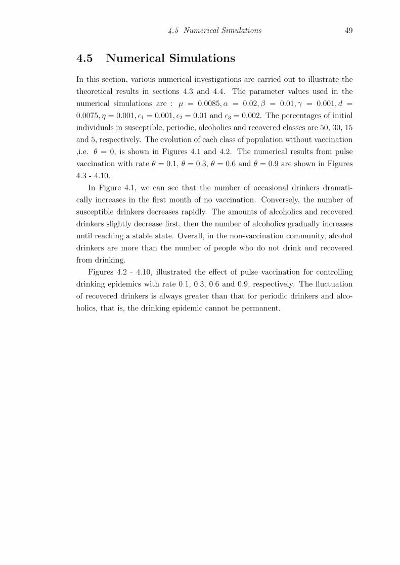
4.5 Numerical Simulations 49
4.5 Numerical Simulations
In this section, various numerical investigations are carried out to illustrate the
theoretical results in sections 4.3 and 4.4. The parameter values used in the
numerical simulations are : µ = 0.0085, α = 0.02, β = 0.01, γ = 0.001, d =
0.0075, η = 0.001, ε1 = 0.001, ε2 = 0.01 and ε3 = 0.002. The percentages of initial
individuals in susceptible, periodic, alcoholics and recovered classes are 50, 30, 15
and 5, respectively. The evolution of each class of population without vaccination
,i.e. θ = 0, is shown in Figures 4.1 and 4.2. The numerical results from pulse
vaccination with rate θ = 0.1, θ = 0.3, θ = 0.6 and θ = 0.9 are shown in Figures
4.3 - 4.10.
In Figure 4.1, we can see that the number of occasional drinkers dramati-
cally increases in the first month of no vaccination. Conversely, the number of
susceptible drinkers decreases rapidly. The amounts of alcoholics and recovered
drinkers slightly decrease first, then the number of alcoholics gradually increases
until reaching a stable state. Overall, in the non-vaccination community, alcohol
drinkers are more than the number of people who do not drink and recovered
from drinking.
Figures 4.2 - 4.10, illustrated the effect of pulse vaccination for controlling
drinking epidemics with rate 0.1, 0.3, 0.6 and 0.9, respectively. The fluctuation
of recovered drinkers is always greater than that for periodic drinkers and alco-
holics, that is, the drinking epidemic cannot be permanent.

4.5 Numerical Simulations 50
Figure 4.1: The evolutions of the four classes of populations without vaccination.
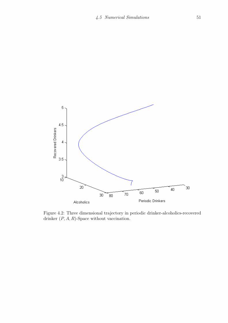
4.5 Numerical Simulations 51
Figure 4.2: Three dimensional trajectory in periodic drinker-alcoholics-recovereddrinker (P,A,R)-Space without vaccination.
4.5 Numerical Simulations 52
Figure 4.3: The evolutions of the four classes of populations with pulse vaccinationrate θ = 0.1.
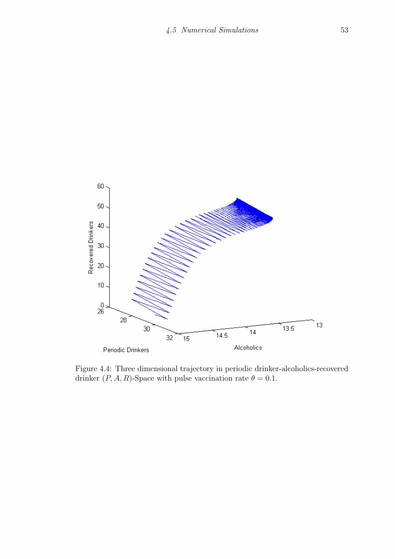
4.5 Numerical Simulations 53
Figure 4.4: Three dimensional trajectory in periodic drinker-alcoholics-recovereddrinker (P,A,R)-Space with pulse vaccination rate θ = 0.1.

4.5 Numerical Simulations 54
Figure 4.5: The evolutions of the four classes of populations with pulse vaccinationrate θ = 0.3.
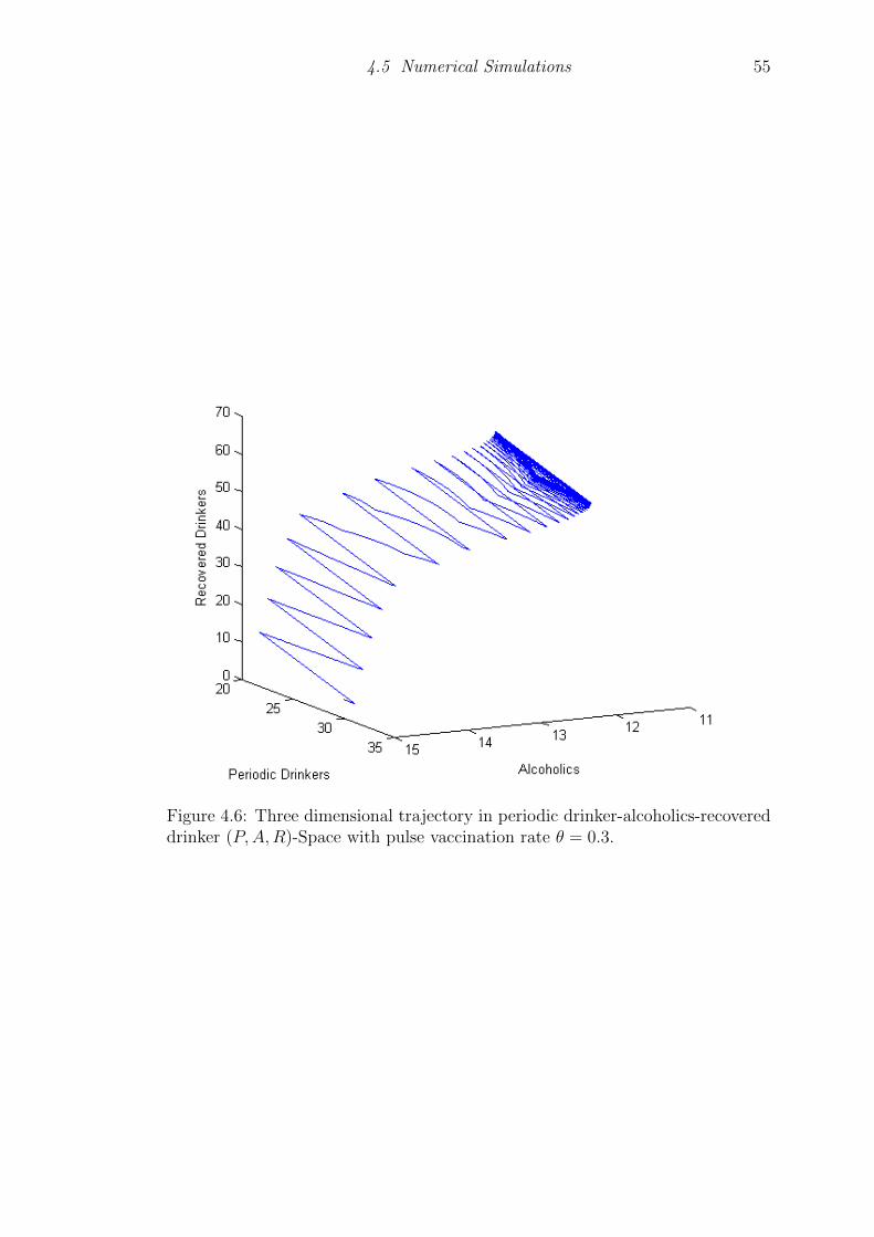
4.5 Numerical Simulations 55
Figure 4.6: Three dimensional trajectory in periodic drinker-alcoholics-recovereddrinker (P,A,R)-Space with pulse vaccination rate θ = 0.3.

4.5 Numerical Simulations 56
Figure 4.7: The evolutions of the four classes of populations with pulse vaccinationrate θ = 0.6.

4.5 Numerical Simulations 57
Figure 4.8: Three dimensional trajectory in periodic drinker-alcoholics-recovereddrinker (P,A,R)-Space with pulse vaccination rate θ = 0.6.

4.5 Numerical Simulations 58
Figure 4.9: The evolutions of the four classes of populations with pulse vaccinationrate θ = 0.9.
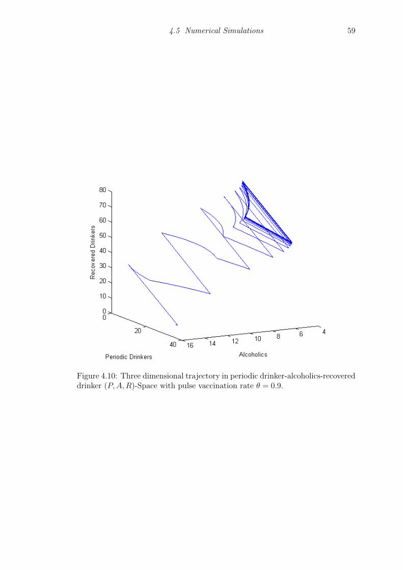
4.5 Numerical Simulations 59
Figure 4.10: Three dimensional trajectory in periodic drinker-alcoholics-recovereddrinker (P,A,R)-Space with pulse vaccination rate θ = 0.9.

4.6 Concluding Remarks 60
4.6 Concluding Remarks
In this chapter, we have studied the dynamical behavior of a drinking epidemic
model with two time-delays and impulsive vaccination. Two thresholds R∗ and
R∗ are derived and it is shown that if R∗ < 1 then the drinking will disappear,
while if R∗ > 1 then the drinking will be permanent which means that after
some period of time the drinking will become hazardous. Analytical expression
of three critical values θ∗, ω∗ and τ ∗ have been established and it is shown that
θ > θ∗ or ω > ω∗ or τ > τ ∗ implies that the drinking will eradicate, while θ < θ∗
or ω < ω∗ implies that the drinking will be uniformly persistent. The research
indicates that the long latent period of drinking or a long recovered period or a
large pulse vaccination rate will lead to eradication of drinking.

CHAPTER 5
Summary and Further Research
5.1 Summary
In this thesis, we have investigated a mathematical model describing the dynamics
of drinking. This model consists of four differential equations describing the rate
of change for four subpopulation S, P , A and R. We investigated the stability
of the model and have demonstrated that the model is asymptotically stable.
Furthermore, we studied two strategies to eradicate the drinking epidemic and
investigate the optimal control of treatment and impulsive vaccination. Based on
previous work in the field, some new analytical and numerical results have been
derived. The main results are summarized as follows:
(1) Results for the stability analysis of the SPARS drinking epidemic model
(i) The threshold quantity that determines the average number of secondary
drinkers produced when one drinker individual is introduced into a group of
susceptible individuals, the basic reproduction number, is R0 = αµd(d+β+ε1)
where α
is the contact rate, µ is the rate of the general population entering the susceptible
population, d is the natural death rate , β is the proportion becoming alcoholic
and ε1 is the death rate of occasional drinkers.
(ii) From the investigation, it can be concluded that the drinking free equilib-
rium is stable if R0 < 1, or otherwise unstable. Moreover, persistent drinking is
always stable. The model was shown to be stable, which is an important feature
of a good model.
(iii) Numerical simulation has been carried out and the results have confirmed
the verification of analytical results.
61

5.2 Further Research 62
(2) Results for the optimal control strategy
(i) An optimal control strategy has been established to minimize the number
of drinkers, including occasional drinkers and alcoholics, and to maximize the
number of recovered individuals.
(ii) Numerical simulations show that, under the optimal control strategy, the
numbers of periodic drinkers and the alcoholic individuals decrease while the
numbers of recovered group and total population increase in the optimality sys-
tem.
(3) Results for the impulsive vaccination.
(i) Based on the mathematical model constructed, we investigated the drink-
ing epidemic model with two time-delays and impulsive vaccination. The pulse
term is (1 − θ)S(t), which means that the vaccination is applied every T time
interval and θ ∈ (0, 1) denotes the proportion of successful vaccination.
(ii) By analysing the SPARS model, two thresholds have been established,
one for global interactivity of the drinking-free solution and another for the per-
manence of drinking solution.
(iii) As summarized in Corollaries 4.5 and 4.8, drinking disappears when θ >
θ∗ whereas drinking persists when θ < θ∗ where θ∗ and θ∗ are shown in Corollaries
4.5 and 4.8, respectively.
(iv) Our results indicate that a long latent period of the disease or a large
pulse vaccination rate will lead to eradication of drinking.
5.2 Further Research
In this project, we minimize the number of drinkers by finding the optimal control
for the drinking epidemic model with numerical verification of the results with
the corresponding parameters to the thresholds. Using real data to demonstrate
how the optimal control theory can be applied in real situation will be continued
in future research. One possible extension is to consider the optimal control
strategy of the SPARS drinking epidemic model with time delay. Moreover,
the two epidemic control strategies, namely the optimal control and impulsive
vaccination, may be extended to study other epidemics.

Bibliography
[1] McGraw-Hill Science and Technology Encyclopedia. website:
http://www.answers.com/topic/epidemiology, August,2011.
[2] N.Bailey. The Mathematical Theory of Infectious Diseases. Charles Griffrin,
1975.
[3] R.M.Anderson, R.M.May, and B.Anderson. Infectious Diseases of Humans:
Dynamics and Control. Oxford Science Publications, 1992.
[4] J.D.Murray. Mathematical Biology I and II. Springer, 2004.
[5] F.Brauer and C.Castillo-Chavez. Mathematical Models in Population Biology
and Epidemiology. 2. Springer, 2010.
[6] E.White and C.Comisky. Heroin epidemics, treatment and ODE modeling.
Mathematical Biosciences, 208:312324, 2007.
[7] G.Mulone and B.Straughan. A note on heroin epidemics. Mathematical
Biosciences, 218:138–141, 2009.
[8] P.Munz, I.Hudea, J.Imad, and R.J.Smith. When Zombies Attack!: Mathe-
matical Modelling of an Outbreak of Zombie Infection. Nova Science Pub-
lishers, 2009.
[9] G.Zaman, Y.H.Kang, and I.H.Jung. Stability analysis and optimal vaccina-
tion of an SIR epidemic model. BioSystems, 93(3):240–249, 2008.
[10] F.Sanchez, C.Castillo-Chvez, D.M.Gorman, and P.Gruenewald. Drinking
as an epidemic: A simple mathematical model with recovery and relapse.
Academic Press, New York, 2007.
[11] B.Benedict. Modeling alcoholism as a contagious disease: how infected drink-
ing buddies spread problem drinking. SIAM News, 40(3), 2007.
[12] P.Newman. Modelling alcoholism as an epidemic. PhD thesis, Durham
University, 2008.
63
[13] J.L.Manthey, A.Y.Aidoo, and K.Y.Ward. Campus drinking: an epidemio-
logical model. Journal of Biological Dynamics, 2(3):346–356, 2008.
[14] E.S.Allman and A.R.John. Mathemaical Models in Biology - An Introuction.
Cambridge University Press, New York, 2004.
[15] W.Kermack and A.McKendrick. A contribution to the mathematical theory
of epidemics. Proceedings of the Royal Society A, 115:700–721, 1927.
[16] J.Mena-Lorca and H.W.Hethcote. Dynamic models of infectious diseases as
regulators of population sizes. Journal of Mathematical Biology, 30:693–716,
1992.
[17] W.M.Liu, H.W.Hethcote, and S.A.Levin. Dynamical behavior of epidemio-
logical models with nonlinear incident rates. Journal of Mathematical Biol-
ogy, 25:359–380, 1987.
[18] D.Greenhalgh. Some result for an SEIR epidemic model with density depen-
dence in the death rate. IMA Journal of Mathematics Applied in Medicine
and Biology, 9(2):67–106, 1992.
[19] J.Zhang and Z.Ma. Global dynamics of an SEIR epidemic model with satu-
rating contact rate. Mathematical Biosciences, 185:15–32, 2003.
[20] L.S.Pontryagin, V.G.Boltyanskii, R.V.Gamkrelize, and E.F.Mishchenko.
The Mathematical Theory of Optimal Processes.
[21] S.Lenhart and J.T.Workman. Optimal Control Applied to Biological Model.
Chapman & Hall CRC Mathematics and Computational Biology. Taylor &
Francis Group, 2007.
[22] C.Castilho. Optimal control of an epidemic through educational campaigns.
Electronic Journal of Differential equations, 2006(125):1–11, 2006.
[23] N.G.Becker and D.N.Starczak. Optimal vaccination strategies for a commu-
nity of households. Mathematical Biosciences, 139(2):117–132, 1997.
[24] M.L.Brandeau, G.S.Zaric, and A.Richter. Resource allocation for control
of infectious diseases in multiple independent populations: beyond cost-
effectiveness analysis. Journal of Health Economics, 22(4):575–598, 2003.
[25] K.Wickwire. Mathematical models for the control of pests and infectious
diseases. Theoretical Population Biology, 11(2):182–238, 1977.
64

[26] K.R.Fister, S.Lenhart, and J.S.McNally. Optimizing chemotherapy in an
HIV model, electronic journal of differential equations. Electronic Journal
of Differential Equations, 1998(32):1–12, 1998.
[27] D.Krischner, S.Lenhart, and S.Serbin. Optimal control of the chemotherapy
of HIV. Journal of Mathematical Biology, 35(7):775–792, 1997.
[28] H.R.Joshi. Optimal control of an HIV immunology model. Optimal Control
Applications and Methods, 23(4):199–213, 2002.
[29] Y.H.Kang, S.Lenhart, and V.Protopopescu. Optimal control of parameters
and input functions for nonlinear systems. Houston Journal of Mathematics,
33(4):1231–1256, 2007.
[30] K.Dietz and D.Schenzle. A Celebration of Statistics. ISI Centenary. Springer,
1985. A Celebration of Statistics.
[31] E.D.Wiraningsih, W.L.Aryati, S.Toaha, and S.Lenhart. Optimal control
for seir rabies model between dogs and human with vaccination effect in
dogs. Proceedings of the 6th IMT-GT Conference on Mathematics, Statistics
and its Applications (ICMSA 2010) Universiti Tunku Abdul Rahman, Kuala
Lumpur,Malaysia, pages 1161–11759, 2010.
[32] D.D.Bainov, A.B.Dishiev, and I.M.Stamova. Lipschitz quasistability of im-
pulsive differential-difference equations with variable impulsive perturbation-
s. Journal of Computational and Applied Mathematics, 70:267–277, 1996.
[33] K.G.Dishlieva. Differentiability of solutions of impulsive differential equa-
tions with respect to the impulsive perturbations. Nonlinear Analysis: Real
World Applications, 12(6):3541–3551, 2011.
[34] K.G.Dishlieva. Continuous dependence of the solutions of impulsive differen-
tial equations on the initial conditions and barrier curves. Acta Mathematica
Scientia, 32(3):1035–1052, 2012.
[35] A.Samoilenko and N.Perestyuk. Differential equations with impulsive per-
turbations. 1987.
[36] V.Lakshmikantham, D.D.Bainov, and P.S.Simeonov. Theory of impulsive
differential equations. Singapore : World Scientific, 1989.
65
[37] G.Z.Zeng, L.S.Chen, and L.H.Sun. Complexity of an SIR epidemic dynamics
model with impulsive vaccination control. Chaos, Solitons and Fractals,
26:495–505, 2005.
[38] X.B.Zhang, H.F.Huo, and Q.Fu. The differential susceptibility sir epidemic
model with stage structure and pulse vaccination. Nonlinear Analysis: Real
World Applications, 11:2634–2646, 2010.
[39] R.Shi, X.Jiang, and L.Chen. The effect if impulsive on an SIR epidemic
model. Applied Mathematics and Computational, 212:305–311, 2009.
[40] J.Li and Y.Yang. SIR-SVS epidemic models with continuous and impulsive
vaccination strategies. Journal of Theoretical Biology, 280:108–116, 2011.
[41] A.d’Onofrio. Mixed pulse vaccination strategy in epidemic model with re-
alistic distributed infectious and latent times. Applied Mathematics and
Computation, 151(1):181–187, 2000.
[42] A.d’Onofrio. Stability properties of pulse vaccination strategy in SEIR epi-
demic model. Mathematical Biosciences, 179:57–72, 2002.
[43] S.Patten and J.Arboleda-Florez. Epidemic theory and group violence. Social
Psychiatry and Epidemiology, 39(11):853–856, 2004.
[44] A.Noymer. The transmission and persistence of urban legends: sociological
application of age-structured epidemic models. Center for Culture, Organi-
zations and Politics, pages 1–34, 2001.
[45] K.Witkiewitz. Lapses following alcohol treatment: Modeling the falls from
the wagon. Journal of Studies on Alcohol and Drugs, 69(4):594–604, 2008.
[46] Centers for Disease Control and Prevention. Alcohol and pub-
lic health. website: http://www.cdc.gov/alcohol/fact-sheets/moderate-
drinking.htm, May,2014.
[47] J.H.Jones. Note on R0, department of anthropological sciences, stanford
university. website : http://www.stanford.edu/ jhj1/teachingdocs/Jones-on-
R0.pdf, August,2011.
[48] L.Edelstein Keshet. Mathematical Models in Biology. Random House, New
York, 1988. SIAM edition.
66

[49] G.Birkhoff and G.C.Rota. Ordinary Differential Equations. The Random
House Group, 1989. Birkhauser Mathematics Series.
[50] W.H.Fleming and R.W.Rishel. Deterministic and Stochastic Optimal Con-
trol. Springer Verlag, New York, 1975.
[51] D.L.Lukes. Differential equations: Classical to controlled. Mathematics in
Science and Engineering, 162:182, 1982.
[52] J.Hou and Z.Teng. Continuous and impulsive vaccination of SEIR epidem-
ic models with saturation incidence rates. Mathematics and Computers in
Simulation, 79:3038–3054, 2009.
[53] Z.Yang and H.Jia. Epidemic dynamics model with delay and impulsive vac-
cination control base on variable population. Mathematical Methods in the
Applied Sciences, 34:1822–1832, 2011.
[54] B.Shulgin, L.Stone, and Z.Agur. Theoretical examinations of pulse vac-
cination policy in the SIR epidemic model. Mathematical and Computer
Modelling, 30:207–215, 2004.
[55] Z.Agur, L.Cojocaru, G.Mazor, R.M.Anderson, and Y.L.Danon. Pulse
measles vaccination across age cohorts. Proceeding of the National Academy
of Sciences of the United States of America, 90(24):11698–11702, 1993.
[56] J.Hui and L.Chen. Impulsive vaccination of SIR epidemic models with non-
linear incidence rates. Discrete and Continuous Dynamical systems- Series
B, 4(3):595–605, 2004.
[57] S.Gao, L.Chen, and Z.Teng. Pulse vaccination of an SEIR epidemic model
with time delay. NonlinearAnalysis : Real World Applications, 9:599–607,
2008.
[58] C.Hsu. New & quot; alcoholism vaccine & quot; gives drinkers instant
hangovers after just one sip. website: http://www.medicaldaily.com/new-
alcoholism-vaccine-gives-drinkers-instant-hangovers-after-just-one-sip-
244391, January, 2013.
[59] E.Beretta, T.Hara, W.B.Ma, and Y.Takeuchi. Global asymptotic stability
of an SIR epidemic model with distributed time delay. Nonlinear Analysis
Theory Methods and Applications, 47:4107–4117, 2001.
67

[60] McCluskey and C.Connell. Global stability of an SIR epidemic model with
delay and general nonlinear incidence. Mathematical Biosciences and Engi-
neering, 7(4):837–850, 2010.
[61] Y.Takeuchi, W.B.Ma, and E.Beretta. Global asymptotic properties of a
delay SIR epidemic model with finite in cubation times. Nonlinear Analysis
Theory Methods and Applications, 42(4):931–947, 2000.
[62] K.Cooke and P.van den Driessche. Analysis of an SEIRS epidemic model
with two delays. Journal of Mathematical Biology, 35:240–260, 1996.
[63] W.Wang. Global behavior of an SEIRS epidemic model with time delays.
Applied Mathematics Letters, 15(4):423–428, 2002.
[64] M.Langlais. A remark on a generic SEIRS model and application to cat
retrovirusese and fox rabies. Mathematical and Computer Modelling, 31:117–
124, 2000.
[65] J.Li and Z.Jin. Global stability of a SEIR epidemic model with infectious
force in latent, infected and immune period. Chaos Solitons and Fractals,
25:1177–1184, 2005.
[66] Y.Michael, H.Smith, and L.Wang. Global dynamics of an SEIR epidem-
ic model with vertical transmission. SIAM Journal Applied Mathematics,
62(1):58–69, 2001.
[67] H.W.Hethcote, H.W.Stech, and P.Van den Driessche. Periodicity and stabil-
ity in epidemic models. Applied Mathematical Ecology. Springer, New York,
1989.
[68] X.Wang, Y.Tao, and X.Song. Pulse vaccination onSEIR epidemic model with
nonlinear incidence rate. Applied Mathematics and Computation, 210:398–
404, 2009.
[69] Z.Zhao, L.Chen, and X.Song. Impulsive vaccination of SEIR epidemic model
with time delay and nonlinear incidence rate. Mathematics amd Computers
in Simulation, 79:500–510, 2008.
[70] R.Xu. Global stability of delayed epidemic model with latent period and
vaccination strategy. Applied Mathematical modelling, 36:5293–5300, 2012.
68

[71] H.Wei, Y.Jiang, X.Song, G.H.Su, and S.Z.Qiu. Global attractivity and per-
manence of a SVEIR epidemic model with pulse vaccination and time delay.
Journal of Computational and Applied Mathematics, 229:302–312, 2009.
[72] T.Zhang and Z.Tang. Pulse vaccination delayed SEIRS epidemic model with
saturation incidence. Applied Mathematical Modelling, 32:1403–1416, 2008.
[73] S.Gao, L.Chen, J.J.Nieto, and A.Torres. Analysis of delayed epidemic model
with pulse vaccination and saturation incidence. Vaccine, 24:6037–6045,
2006.
[74] T.Zhang and Z.Tang. Global asymptotic stability of a delayed SEIRS
epidemic model with saturation incidence. Chaos, Solitons and Fractals,
37:1456–1468, 2008.
[75] S.Gao, L.Chen, and Z.Teng. Impulsive vaccination of an SEIRS model with
time delay and varying total population size. Bulletin of Mathematical Bi-
ology, 69:731–745, 2007.
[76] X.Meng, L.Chen, and H.Cheng. Two profitless delays for the seirs epidem-
ic disease model with nonlinear incidence and pulse vaccination. Applied
Mathematics and Computational, 186:516–529,, 2007.
[77] S.Gao, Z.Teng, and D.Xie. The effects of pulse vaccination on SEIR model
with two time delays. Applied Mathematics and Computation, 201:282–292,
2008.
[78] Y.Kuang. Delay Differential Equation with Application in Population Dy-
namics. Mathematics in Science and Engineering. Academic Press, 1993.
[79] Y.Xiao and L.Chen. Modelling and analysis of a predator-prey model with
disease in the prey. Mathematical Bioscience, 171(1):59–82, 2001.
[80] T.Zhang and Z.Tang. Extinction and permanence for a pulse vaccination
delayed SEIRS epidemic model. Chaos, Solitons and Fractals, 39(5):2411–
2425, 2009.
Every reasonable effort has been made to acknowledge the owners of copyright
material. I would be pleased to hear from any copyright owner who has been
omitted or incorrectly acknowledged.
69


![GLOBAL STABILITY AND UNIFORM PERSISTENCE …1701.01407v1 [math.AP] 5 Jan 2017 GLOBAL STABILITY AND UNIFORM PERSISTENCE OF THE REACTION-CONVECTION-DIFFUSION CHOLERA EPIDEMIC MODEL KAZUO](https://img.pdfslide.net/doc/110x75/5ad6051b7f8b9a0d2d8e67d7/global-stability-and-uniform-persistence-170101407v1-mathap-5-jan-2017-global.jpg)