STABILITY ANALYSIS OF STIFFENED PANELS ...web.mscsoftware.com/events/aero2002/partner/pdf/p16401.pdfStability Analysis of S tiffened Panels / Analytical and Finite Element Methods

Copyright © 2002 by Pechiney Aerospace. Published by MSC Software., with permission.

MSC-2001-164

STABILITY ANALYSIS OF STIFFENED PANELS

ANALYTICAL AND FINITE ELEMENT METHODS

Raphael Muzzolini1, Sjoerd van der Veen2, Alexis Perez-Duarte3, Jean-Christophe Ehrström1

Abstract The design of large parts of an airframe is driven by post buckling stability requirements. The aim of the present work is to compare stability predictions obtained both by analytical and numerical methods. A study on the sensitivity of this method to material law has also been conducted. This way, the extent to which the precise shape of an high performance aluminium alloy stress / strain curve has an impact on stability results has been evaluated. Compression studies lead to acceptable differences between methods. The trend is however depending on the model : numerical calculations predict lower critical loads as well as upper ones. The field of improvement is undoubtedly modelling methods such as the introduction of a perturbation in the mesh and boundary conditions. More work is needed to better understand these differences. The study of the influence of the material also shows differences between both methods. Little changes are found when using detailed material model with analytical computations whereas FEA do demonstrate room for improvement by using real material data.

1 Researcher, Pechiney Centre de Recherches de Voreppe, corresponding author: [email protected] 2 Development Engineer, Pechiney Aerospace, France 3 Graduate student Department of Aerospace Engineering - University of Michigan, USA / Intern Pechiney Centre de

Recherches de Voreppe, France, Mar – Jul 2001

Introduction The design of large structural parts of an airframe is driven by post-buckling stability requirements. This often consists in the determination of critical loads of stiffened panels in compression. Stability Analysis in Design Aircraft manufacturers use analytical-empirical methods of analysis for this type of problem, because these methods allow a large number of computations in a small amount of time. Their capability of predicting true component behaviour has been evaluated and corrected using a large number of experiments. FEA, Relevance of Present Work An alternative to these analytical-empirical calculations is Finite Element Analysis (FEA). The major drawback of this method for the analysis of components is that it is time consuming: running a simulation can take up to one day, which is unacceptable for swift design iteration. However, the computational delays are continually decreasing due to the growing speed of processors and the increased efficiency of solvers. Moreover,

for complex analysis (including for example shear, compression and lateral pressure) FEA is the only method available. Besides a better representation of the boundary conditions, FEA also allows for more detailed modelling of the geometry and the material behaviour. Applying it therefore allows designers to work with less margin, thus enabling them to reduce the over-weight of the structure. However, if design safety margins are to be reduced, knowing the sensitivity of the methods and models to their input becomes increasingly important. Objective of Present Work The aim of the present work is to compare stability predictions from analytical-empirical methods to results obtained through FEA for pure compression. The present work being undertaken by an airframe material supplier, the sensitivity of both methods to the aluminium constitutive material model is investigated in detail.

Stability Analysis of Stiffened Panels / Analytical and Finite Element Methods

2

Methods Used For the analytical-empirical analysis of the stiffened panel subject to compression only, Euler-Johnson (see appendix) was used. For the evaluation of the influence of the material model, the calculation effort was reduced by applying not the full set of Euler-Johnson curves, but by computing the effective width and calculating the critical stress of the effective section with the Euler-Engesser formula. A summary of conventional compression analysis is given in the appendix. For all FEA, MSC MARC® was employed, using a fine mesh of QUAD shell elements (MARC type 75). The number of layers per shell was set to 11 in the first model and 5 in the second one (after having investigated its influence which was found negligible). Large displacements and large strains methods were used (total Lagrange procedure for elasticity and mean normal method for plasticity). The Hardware Direct Sparse solver, optimized for SGI machines, has been chosen. The Full Newton-Raphson algorithm was used for the resolution of the non linear system. The Arc Length Method was not used. The software was run on a 2 Gbit, 12 processors SGI PowerChallenge machine. The computational time went from 1 hour up to 10 hours depending on the configuration. The model without frames contains 4200 elements and the complete panel 4800. A small step of 0.01 mm per increment was needed for convergence. A perturbation mode is available in MSC MARC® that enables the introduction of a defect in the mesh to facilitate convergence in buckling calculations. After a small initial displacement, a linear bifurcation analysis is performed that calculates the first buckling modes (in the form of nodal displacements). These displacements are normalized, scaled down and applied to the mesh. The displacement driven simulation is then continued up to panel collapse.

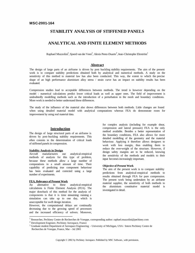
Complete stiffened panel The first model used for the comparative study is represented on Figure 1. It is stiffened both transversally (frames and stabilisers) and longitudinally (stringers). This level of detail is needed for complex studies such as introduction as shear in the load set (shear+compression+ pressure for instance)

92mm

8 mm

6 mm

6 mm

frame

18mm

2 mm

41mm

8 mm

2,5 mm

10 mm

stringer stabiliser

Figure 1

Overview and sections of complete panel model. Stringer pitch: 150 mm, frame pitch: 635 mm, skin thickness 2 mm, no lands Modelling The junction between stiffeners and skin has been modelled only by playing with thickness. For the shells representing skin + stiffener foot, thickness has been set to the sum of both elements thickness.

Stringers

Frames

Stabilisers


3

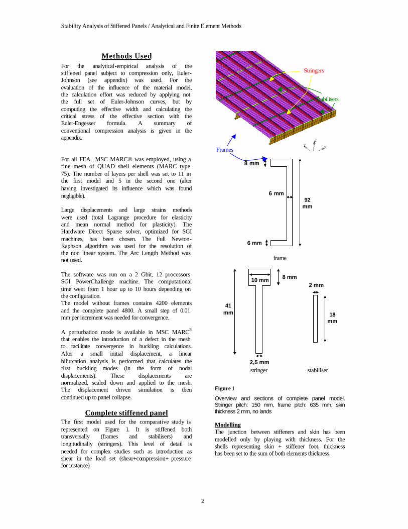
MARC perturbation mode has been used with a reduction factor of 10, leading to perturbation displacements in the order of 6 % of the skin thickness. Buckling is a severe change of direction in the force vs displacement curve and thus numerical computations can easily diverge. To avoid some problems already encountered in other models, the edges of our model have been artificially rigidified as illustrated in Figure 2. The Young’s Modulus used for the rigid material is approximately 10 times higher. The size of the domain is equivalent to one bay (the zone between 2 frames), half a bay on each side of the panel.

Figure 2

Artificially rigidifying edges The introduction of rigid zones softens the constraints linked to clamped boundary conditions. A global movement of the rigid zones is indeed permitted whereas the first element on the edge has to remain horizontal in a classical modeling, which is a tough constraint. However, one has to be very careful with this method, because it can lead to higher critical buckling load by artificially rigidifying the panel, yielding design predictions that may not be conservative. Materials In the case of this example, the material properties of skin and stringers were taken Ec = 73 000 MPa, ν = 0.33 and furthermore as given in Figure 3. The frames were made of an alloy with Ec = 73 100 MPa, ν = 0.33 and as given in Figure 3. Ramberg-Osgood parameters used in the analytical-empirical calculations were Fcy = 370 MPa and nc = 15.

300

320

340

360

380

400

420

440

460

480

0% 1% 2% 3% 4% 5% 6 %

Plastic strain (%)

Str

ess

(MP

a)

skin+stringersframes

Figure 3

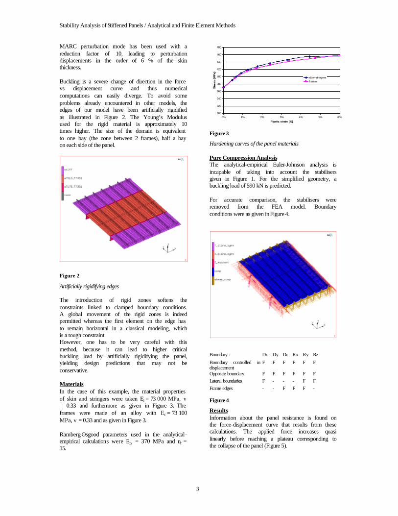
Hardening curves of the panel materials Pure Compression Analysis The analytical-empirical Euler-Johnson analysis is incapable of taking into account the stabilisers given in Figure 1. For the simplified geometry, a buckling load of 590 kN is predicted. For accurate comparison, the stabilisers were removed from the FEA model. Boundary conditions were as given in Figure 4.

Boundary : Dx Dy Dz Rx Ry Rz

Boundary controlled in displacement

F F F F F F

Opposite boundary F F F F F F Lateral boundaries F - - - F F Frame edges - - F F F -

Figure 4

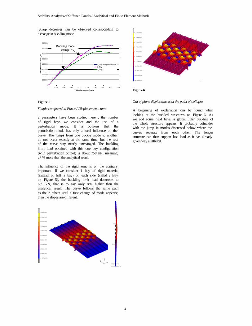
Results Information about the panel resistance is found on the force-displacement curve that results from these calculations. The applied force increases quasi linearly before reaching a plateau corresponding to the collapse of the panel (Figure 5).


4

Sharp decreases can be observed corresponding to a change in buckling mode.

0

100000

200000

300000

400000

500000

600000

700000

800000

- 0.50 1.00 1.50 2.00 2.50 3.00 3.50 4.00 4.50

Y Displacement (mm)

Com

pres

sive

Loa

d (N

)

1_Bay with perturbation1_Bay2_bay

Figure 5

Simple compression Force / Displacement curve 2 parameters have been studied here : the number of rigid bays we consider and the use of a perturbation mode. It is obvious that the perturbation mode has only a local influence on the curve. The jumps from one buckle mode to another do not occur exactly at the same time, but the rest of the curve stay nearly unchanged. The buckling limit load obtained with this one bay configuration (with perturbation or not) is about 750 kN, meaning 27 % more than the analytical result. The influence of the rigid zone is on the contrary important. If we consider 1 bay of rigid material (instead of half a bay) on each side (called 2_Bay on Figure 5), the buckling limit load decreases to 639 kN, that is to say only 8 % higher than the analytical result. The curve follows the same path as the 2 others until a first change of mode appears; then the slopes are different.

Figure 6

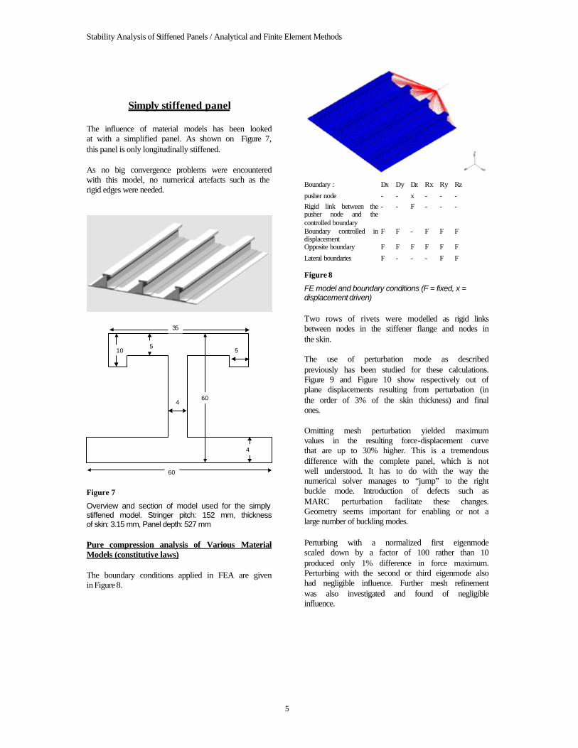
Out of plane displacements at the point of collapse A beginning of explanation can be found when looking at the buckled structures on Figure 6. As we add some rigid bays, a global Euler buckling of the whole structure appears. It probably coincides with the jump in modes discussed below where the curves separate from each other. The longer structure can then support less load as it has already given way a little bit.

Buckling mode change


5

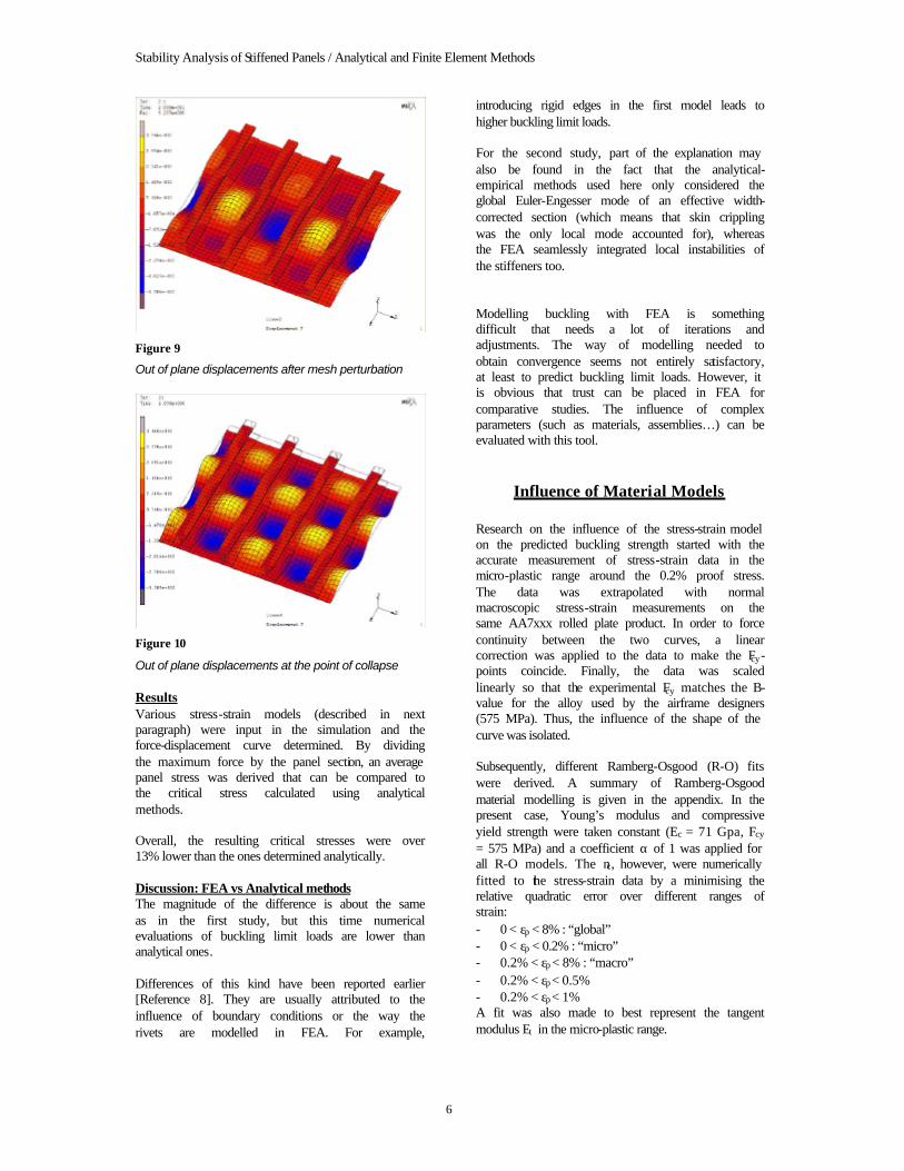
Simply stiffened panel The influence of material models has been looked at with a simplified panel. As shown on Figure 7, this panel is only longitudinally stiffened. As no big convergence problems were encountered with this model, no numerical artefacts such as the rigid edges were needed.

10

35

60

55

4

4

60

Figure 7

Overview and section of model used for the simply stiffened model. Stringer pitch: 152 mm, thickness of skin: 3.15 mm, Panel depth: 527 mm Pure compression analysis of Various Material Models (constitutive laws) The boundary conditions applied in FEA are given in Figure 8.

Boundary : Dx Dy Dz Rx Ry Rz

pusher node - - x - - - Rigid link between the pusher node and the controlled boundary

- - F - - -

Boundary controlled in displacement

F F - F F F

Opposite boundary F F F F F F

Lateral boundaries F - - - F F

Figure 8

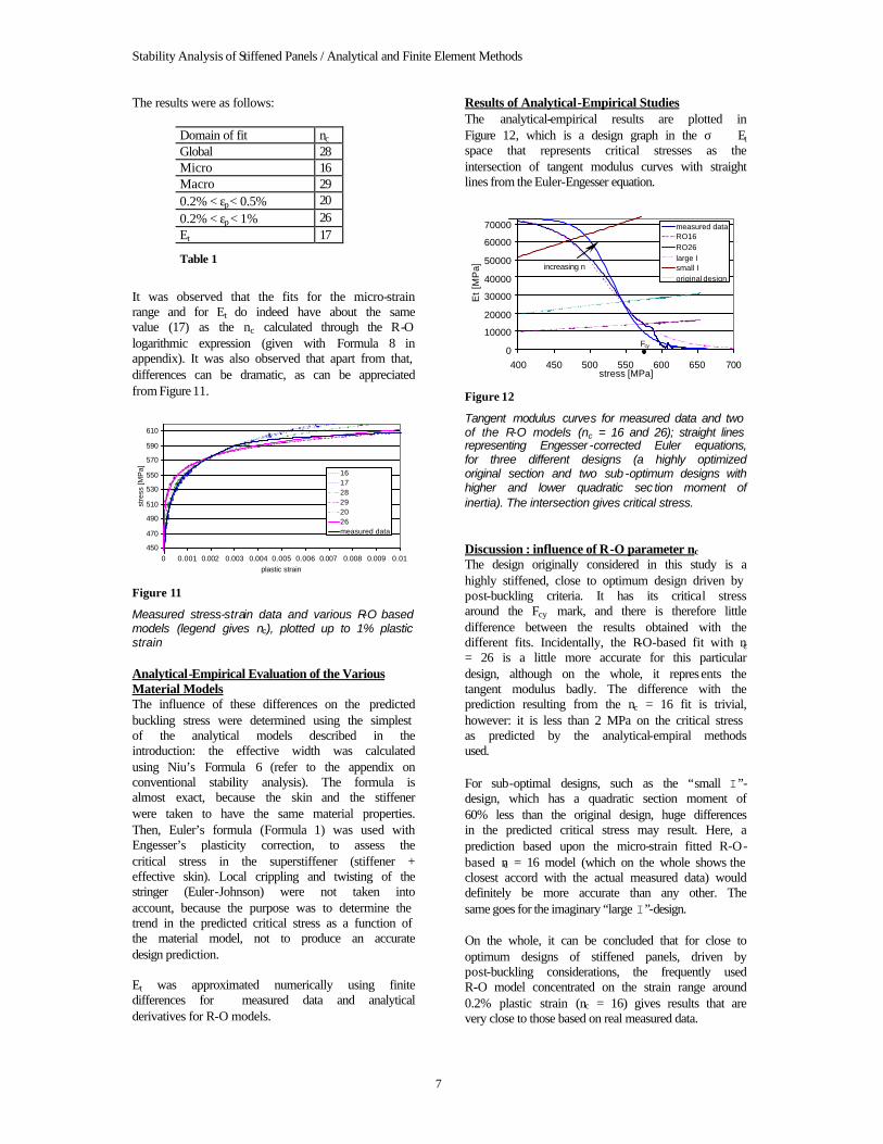
FE model and boundary conditions (F = fixed, x = displacement driven) Two rows of rivets were modelled as rigid links between nodes in the stiffener flange and nodes in the skin. The use of perturbation mode as described previously has been studied for these calculations. Figure 9 and Figure 10 show respectively out of plane displacements resulting from perturbation (in the order of 3% of the skin thickness) and final ones. Omitting mesh perturbation yielded maximum values in the resulting force-displacement curve that are up to 30% higher. This is a tremendous difference with the complete panel, which is not well understood. It has to do with the way the numerical solver manages to “jump” to the right buckle mode. Introduction of defects such as MARC perturbation facilitate these changes. Geometry seems important for enabling or not a large number of buckling modes. Perturbing with a normalized first eigenmode scaled down by a factor of 100 rather than 10 produced only 1% difference in force maximum. Perturbing with the second or third eigenmode also had negligible influence. Further mesh refinement was also investigated and found of negligible influence.


6

Figure 9

Out of plane displacements after mesh perturbation

Figure 10

Out of plane displacements at the point of collapse Results Various stress-strain models (described in next paragraph) were input in the simulation and the force-displacement curve determined. By dividing the maximum force by the panel section, an average panel stress was derived that can be compared to the critical stress calculated using analytical methods. Overall, the resulting critical stresses were over 13% lower than the ones determined analytically. Discussion: FEA vs Analytical methods The magnitude of the difference is about the same as in the first study, but this time numerical evaluations of buckling limit loads are lower than analytical ones. Differences of this kind have been reported earlier [Reference 8]. They are usually attributed to the influence of boundary conditions or the way the rivets are modelled in FEA. For example,

introducing rigid edges in the first model leads to higher buckling limit loads. For the second study, part of the explanation may also be found in the fact that the analytical-empirical methods used here only considered the global Euler-Engesser mode of an effective width-corrected section (which means that skin crippling was the only local mode accounted for), whereas the FEA seamlessly integrated local instabilities of the stiffeners too. Modelling buckling with FEA is something difficult that needs a lot of iterations and adjustments. The way of modelling needed to obtain convergence seems not entirely satisfactory, at least to predict buckling limit loads. However, it is obvious that trust can be placed in FEA for comparative studies. The influence of complex parameters (such as materials, assemblies…) can be evaluated with this tool.

Influence of Material Models Research on the influence of the stress-strain model on the predicted buckling strength started with the accurate measurement of stress-strain data in the micro-plastic range around the 0.2% proof stress. The data was extrapolated with normal macroscopic stress-strain measurements on the same AA7xxx rolled plate product. In order to force continuity between the two curves, a linear correction was applied to the data to make the Fcy-points coincide. Finally, the data was scaled linearly so that the experimental Fcy matches the B-value for the alloy used by the airframe designers (575 MPa). Thus, the influence of the shape of the curve was isolated. Subsequently, different Ramberg-Osgood (R-O) fits were derived. A summary of Ramberg-Osgood material modelling is given in the appendix. In the present case, Young’s modulus and compressive yield strength were taken constant (Ec = 71 Gpa, Fcy = 575 MPa) and a coefficient α of 1 was applied for all R-O models. The nc, however, were numerically fitted to the stress-strain data by a minimising the relative quadratic error over different ranges of strain: - 0 < εp < 8% : “global” - 0 < εp < 0.2% : “micro” - 0.2% < εp < 8% : “macro” - 0.2% < εp < 0.5% - 0.2% < εp < 1% A fit was also made to best represent the tangent modulus Et in the micro-plastic range.


7

The results were as follows:

Domain of fit nc

Global 28 Micro 16 Macro 29 0.2% < εp

< 0.5% 20 0.2% < εp < 1% 26 Et 17

Table 1

It was observed that the fits for the micro-strain range and for Et do indeed have about the same value (17) as the nc calculated through the R-O logarithmic expression (given with Formula 8 in appendix). It was also observed that apart from that, differences can be dramatic, as can be appreciated from Figure 11.

450

470

490

510

530

550

570

590

610

0 0.001 0.002 0.003 0.004 0.005 0.006 0.007 0.008 0.009 0.01plastic strain

stre

ss [M

Pa] 16

1728292026measured data

Figure 11

Measured stress-strain data and various R-O based models (legend gives nc), plotted up to 1% plastic strain Analytical-Empirical Evaluation of the Various Material Models The influence of these differences on the predicted buckling stress were determined using the simplest of the analytical models described in the introduction: the effective width was calculated using Niu’s Formula 6 (refer to the appendix on conventional stability analysis). The formula is almost exact, because the skin and the stiffener were taken to have the same material properties. Then, Euler’s formula (Formula 1) was used with Engesser’s plasticity correction, to assess the critical stress in the superstiffener (stiffener + effective skin). Local crippling and twisting of the stringer (Euler-Johnson) were not taken into account, because the purpose was to determine the trend in the predicted critical stress as a function of the material model, not to produce an accurate design prediction. Et was approximated numerically using finite differences for measured data and analytical derivatives for R-O models.

Results of Analytical-Empirical Studies The analytical-empirical results are plotted in Figure 12, which is a design graph in the σ Et space that represents critical stresses as the intersection of tangent modulus curves with straight lines from the Euler-Engesser equation.

0

10000

20000

30000

40000

50000

60000

70000

400 450 500 550 600 650 700stress [MPa]

Et

[MP

a]

measured dataRO16RO26large Ismall Ioriginal design

Figure 12

Tangent modulus curves for measured data and two of the R-O models (nc = 16 and 26); straight lines representing Engesser -corrected Euler equations, for three different designs (a highly optimized original section and two sub -optimum designs with higher and lower quadratic sec tion moment of inertia). The intersection gives critical stress. Discussion : influence of R-O parameter nc The design originally considered in this study is a highly stiffened, close to optimum design driven by post-buckling criteria. It has its critical stress around the Fcy mark, and there is therefore little difference between the results obtained with the different fits. Incidentally, the R-O-based fit with nc = 26 is a little more accurate for this particular design, although on the whole, it repres ents the tangent modulus badly. The difference with the prediction resulting from the nc = 16 fit is trivial, however: it is less than 2 MPa on the critical stress as predicted by the analytical-empiral methods used. For sub-optimal designs, such as the “small I”-design, which has a quadratic section moment of 60% less than the original design, huge differences in the predicted critical stress may result. Here, a prediction based upon the micro-strain fitted R-O-based nc = 16 model (which on the whole shows the closest accord with the actual measured data) would definitely be more accurate than any other. The same goes for the imaginary “large I”-design. On the whole, it can be concluded that for close to optimum designs of stiffened panels, driven by post-buckling considerations, the frequently used R-O model concentrated on the strain range around 0.2% plastic strain (nc = 16) gives results that are very close to those based on real measured data.

increasing n

Fcy


8

Incidentally, a fit made for a strain range between 0.2 and 1% produced an even better result for the design under consideration (nc = 26); for less optimized designs, however, significant inaccuracies would have occurred for this fit. With the habitual methods of calculating the exponent nc (Formula 8 or Formula 9), the risk of something similar happening may exist; all depends on the two σ-ε-points chosen in the expressions for nc. This risk can be avoided by numerically fitting nc to the tangent modulus derived directly from the measured stress-strain data. Influence of materials The influence of nc has been investigated separately for analytical and numerical calculations and a large difference was found.

468.0

470.0

472.0

474.0

476.0

478.0

480.0

15 17 19 21 23 25 27 29 31nc

criti

cal s

tress

from

FE

A [M

Pa]

543.5

544

544.5

545

545.5

546

546.5cr

itica

l str

ess:

ana

lytic

al [M

Pa]

FEA analytical-empirical

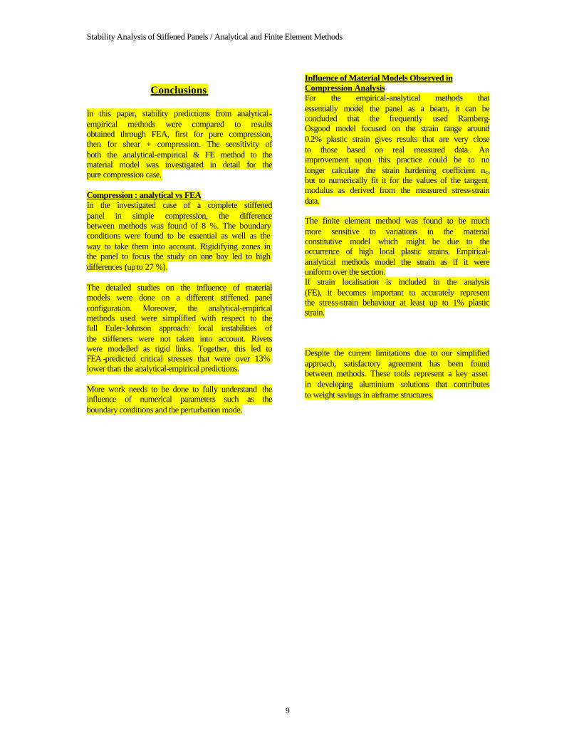
Figure 13

Predicted critical stress as a function of material model (nc), for the post-buckling design given in Figure 7. Note that the critical stresses differences calculated by FEA range over 10 MPa, whereas for analytical -empirical computations, they range over only 3 MPa. Opposite trends can be seen for analytical and numerical methods on Figure 13. The critical stress as predicted by the analytical-empirical methods increases with nc, whereas for FEA, it decreases. The explanation for this probably lies in the amount of plastic strain observed locally, for example in the skin pockets.

0.00%

0.20%

0.40%

0.60%

0.80%

1.00%

1.20%

1.40%

1.60%

0 5 10 15 20 25 30 35

nc (where applicable)

(max

imum

) pl

astic

str

ain

plastic strain analyticalmax.plastic strain FEA

measured data

R-O based fits with varying nc

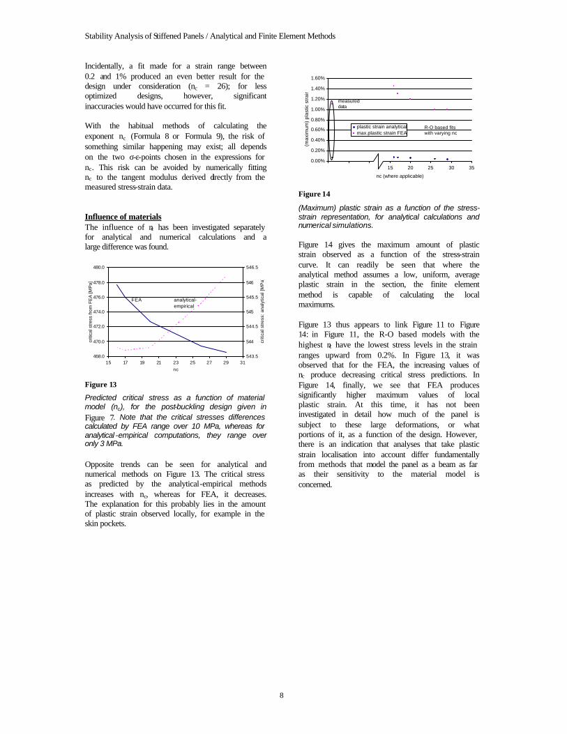
Figure 14

(Maximum) plastic strain as a function of the stress-strain representation, for analytical calculations and numerical simulations. Figure 14 gives the maximum amount of plastic strain observed as a function of the stress-strain curve. It can readily be seen that where the analytical method assumes a low, uniform, average plastic strain in the section, the finite element method is capable of calculating the local maximums. Figure 13 thus appears to link Figure 11 to Figure 14: in Figure 11, the R-O based models with the highest nc have the lowest stress levels in the strain ranges upward from 0.2%. In Figure 13, it was observed that for the FEA, the increasing values of nc produce decreasing critical stress predictions. In Figure 14, finally, we see that FEA produces significantly higher maximum values of local plastic strain. At this time, it has not been investigated in detail how much of the panel is subject to these large deformations, or what portions of it, as a function of the design. However, there is an indication that analyses that take plastic strain localisation into account differ fundamentally from methods that model the panel as a beam as far as their sensitivity to the material model is concerned.


9

Conclusions In this paper, stability predictions from analytical-empirical methods were compared to results obtained through FEA, first for pure compression, then for shear + compression. The sensitivity of both the analytical-empirical & FE method to the material model was investigated in detail for the pure compression case. Compression : analytical vs FEA In the investigated case of a complete stiffened panel in simple compression, the difference between methods was found of 8 %. The boundary conditions were found to be essential as well as the way to take them into account. Rigidifying zones in the panel to focus the study on one bay led to high differences (up to 27 %). The detailed studies on the influence of material models were done on a different stiffened panel configuration. Moreover, the analytical-empirical methods used were simplified with respect to the full Euler-Johnson approach: local instabilities of the stiffeners were not taken into account. Rivets were modelled as rigid links. Together, this led to FEA -predicted critical stresses that were over 13% lower than the analytical-empirical predictions. More work needs to be done to fully understand the influence of numerical parameters such as the boundary conditions and the perturbation mode.

Influence of Material Models Observed in Compression Analysis For the empirical-analytical methods that essentially model the panel as a beam, it can be concluded that the frequently used Ramberg-Osgood model focused on the strain range around 0.2% plastic strain gives results that are very close to those based on real measured data. An improvement upon this practice could be to no longer calculate the strain hardening coefficient nc, but to numerically fit it for the values of the tangent modulus as derived from the measured stress-strain data. The finite element method was found to be much more sensitive to variations in the material constitutive model which might be due to the occurrence of high local plastic strains. Empirical-analytical methods model the strain as if it were uniform over the section. If strain localisation is included in the analysis (FE), it becomes important to accurately represent the stress-strain behaviour at least up to 1% plastic strain. Despite the current limitations due to our simplified approach, satisfactory agreement has been found between methods. These tools represent a key asset in developing aluminium solutions that contributes to weight savings in airframe structures.


10

APPENDIX: Conventional Compression Stability Analysis

Column Buckling To predict buckling instability under pure compression, Euler first gave an analysis derived from linear beam theory [Reference 1]. The idea behind it is that if it is energetically less involved for the beam to bend than to undergo any further axial deformation, buckling will result. The formula he derived is:

2

2

LIE

P ccr

π=

Formula 1

for a simply supported column, with: • Pcr the critical load at which the beam will

buckle • Ec the Young’s modulus of the material

(measured in compression) • I the beam’s quadratic section moment • L the beam’s length The basis of stability analysis has remained unchanged, but Euler’s model for beams has been perfected over the years to account for large deflections, imperfections in the geometry of the beam, eccentric loading and inelastic material behaviour. This last correction approximates the plastic deformation of the material by employing the tangent- rather than the Young’s modulus in Formula 1 (first proposed by Engesser, [1]). Furthermore, for the model to be valid for stiffened panels rather than just beams, it was necessary to take into account the gradual collapse of the built-up section, due to local crippling in skin and stiffener web and flanges. Johnson proposed an empirical correction for this [Reference 2]:

−=c

crcr

crcrcr E

L

2

2

,

, 4

'

1π

ρσ

σσ

Formula 2

with: • σcr the Euler-Johnson critical stress • σcr,cr the crippling stress from:

ii

icrcriicrcr tb

tb ,,,

σσ ∑= , the “weighted

average” of the local critical crippling stresses σcr,cr,i of the different “strips” of which the section is built-up (with bi the width of each strip and ti its thickness). The σcr,cr,i can be calculated using formulae of the type Formula 3 and Formula 7.

• L’ the effective column length, which depends

on the end constraints: k

LL =' , with k the

“end fixety coefficient” – an empirical value for the stiffness of the boundary conditions

• ρ the section radius of gyration, which is the root of the quadratic section moment divided

by the cross section area,AI=ρ

• Ec the Young’s modulus of the material (measured in compression)

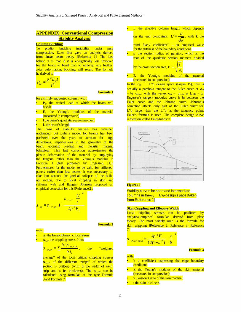
In the σcr L’/ρ design space (Figure 15), this is actually a parabola tangent to the Euler curve at σcr = ½ σcr,cr, with the vertex σcr = σcr,cr at L’/ρ = 0. Engesser’s tangent modulus curve is in between the Euler curve and the Johnson curve. Johnson’s correction affects only part of the Euler curve: for L’/ρ larger than the L’/ρ at the tangency point, Euler’s formula is used. The complete design curve is therefore called Euler-Johnson.

Figure 15

Stability curves for short and intermediate columns in the σcr L’/ρ design s pace [taken from Reference 2] Skin Crippling and Effective Width Local crippling stresses can be predicted by analytical-empirical formulae derived from plate theory. The most widely used is the formula for skin crippling [Reference 2, Reference 3, Reference 7]:

2

2

2

, )1(12

⋅

−=− b

tEkskincrcr υ

πσ

Formula 3

with: • k a coefficient expressing the edge boundary

conditions • E the Young’s modulus of the skin material

(measured in compression) • ν Poisson’s ratio of the skin material • t the skin thickness


11

• b the skin width between stringers This is often expressed in the form:

2

,

⋅=− b

tKEskincrcrσ , with

)1(12 2

2

υπ−

= kK

A very conservative approach could then be to simply exclude the skin from the calculation as soon as it crippled. Later, empirical formulae were derived to contribute some of the load carrying capability to the skin, in the form of an “effective width” of skin, which acts as if it were part of the stiffener rather than the skin [e.g. Reference 3]. Von Kármán and Sechler observed from experiments that the ultimate strength of a simply supported sheet was independent of the width of the sheet. This led to an expression for the effective

width that was a function of skincrcr

skincyF

−

−

,σ. Since the

critical stress of the stiffener can be higher than this yield stress, this was later changed to the loading

ratio, skincrcr

skineffectivestiffener

−

+

,

_

σ

σ. Mentally fixing the

stress in the stiffener and the effective skin at a value equal to the critical stress of the stiffener, and then realizing that the effective width will be the width for which the skin will just start to cripple at that stress level, leads to [Reference 2]:

stiffenercre

KEtb

−

=σ

Formula 4

Substituting the equation for σcr,cr-skin given above yields:

stiffenercr

skincrcre bb

−

−=σ

σ ,

Formula 5

for σ > σcr,cr-skin, and

bbe = for σ = σcr,cr-skin, with:

• be the effective skin width • b the skin width between stringers • σnom the nominal compressive stress in the

stiffened panel To correct for plasticity in the skin, [Reference 2] suggests to use the tangent modulus instead of Young’s modulus:

stiffenercr

te

KEtb

−

=σ

Formula 6

This is of course not entirely correct: plastic crippling of the skin, depending on the boundary conditions, should in fact be calculated through formulae of the type [e.g. Reference 6, Reference 7]:

2

2

2

, )1(12

⋅

−=− b

tEk

p

pskincrcr

υ

πσ

Formula 7

for simply supported edges, with:

++=

s

tsp E

EEE

31

41

21

and

EEs

p

−−= υυ

21

21

, in which:

• Es the secant modulus • Et the tangent modulus

If, on top of the plastic deformation, the material of the stiffeners varies significantly from that of the skin, an iterative approach should be taken. The method comes down to coupling the strain in the stiffener and the effective skin rather than their stress, then finding the stress in the skin and using that stress to calculate the effective width [Reference 3]. Aircraft manufacturers usually have in-house spread sheets or software that does all this. Stringer Twisting A last type of instability to take into account when analysing stiffened panels in compression is stringer twisting. The reader is kindly referred to Reference 4.


12

APPENDIX: Material Properties Used in Stability Analysis: Ramberg-Osgood

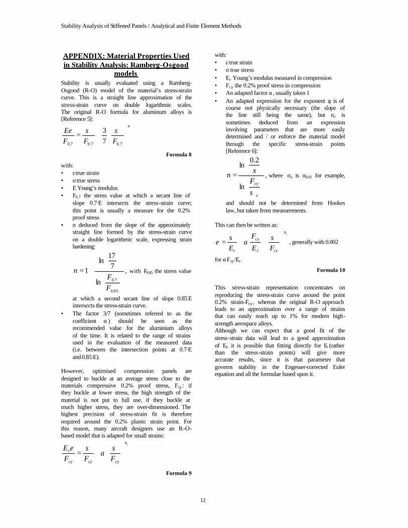
models Stability is usually evaluated using a Ramberg-Osgood (R-O) model of the material’s stress-strain curve. This is a straight line approximation of the stress-strain curve on double logarithmic scales. The original R-O formula for aluminum alloys is [Reference 5]:

n

FFFE

+=

7.07.07.0 73 σσε

Formula 8

with: • ε true strain • σ true stress • E Young’s modulus • F0.7 the stress value at which a secant line of

slope 0.7·E intersects the stress-strain curve; this point is usually a measure for the 0.2% proof stress

• n deduced from the slope of the approximately straight line formed by the stress-strain curve on a double logarithmic scale, expressing strain hardening:

+=

85.0

7.0ln

717

ln1

FF

n , with F0.85 the stress value

at which a second secant line of slope 0.85⋅E intersects the stress-strain curve.

• The factor 3/7 (sometimes referred to as the coefficient α ) should be seen as the recommended value for the aluminium alloys of the time. It is related to the range of strains used in the evaluation of the measured data (i.e. between the intersection points at 0.7·E and 0.85·E).

However, optimised compression panels are designed to buckle at an average stress close to the materials compressive 0.2% proof stress, Fcy : if they buckle at lower stress, the high strength of the material is not put to full use, if they buckle at much higher stress, they are over-dimensioned. The highest precision of stress-strain fit is therefore required around the 0.2% plastic strain point. For this reason, many aircraft designers use an R-O-based model that is adapted for small strains:

cn

cycycy

c

FFFE

+=

σα

σε

Formula 9

with: • ε true strain • σ true stress • Ec Young’s modulus measured in compression • Fcy the 0.2% proof stress in compression • An adapted factor α, usually taken 1 • An adapted expression for the exponent nc is of

course not physically necessary (the slope of the line still being the same), but nc is sometimes deduced from an expression involving parameters that are more easily determined and / or enforce the material model through the specific stress-strain points [Reference 6]:

=

x

cyFxn

σln

2.0ln

, where σx is σ0.01 for example,

and should not be determined from Hookes law, but taken from measurements.

This can then be written as:

cn

cyc

cy

c FE

F

E

⋅+= σασε , generally with 0.002

for αFcy /Ec.

Formula 10

This stress-strain representation concentrates on reproducing the stress-strain curve around the point 0.2% strain-Fcy , whereas the original R-O approach leads to an approximation over a range of strains that can easily reach up to 1% for modern high-strength aerospace alloys. Although we can expect that a good fit of the stress-strain data will lead to a good approximation of Et, it is possible that fitting directly for Et (rather than the stress-strain points) will give more accurate results, since it is that parameter that governs stability in the Engesser-corrected Euler equation and all the formulae based upon it.


13

References

Reference 1

Gere, J.M. & Timoshenko, S.P., Mechanics of Materials, 2nd SI edition, Hong Kong, 1987

Reference 2

Niu, M.C.Y., Airframe Structural Design, 2nd edition, Hong Kong 1999

Reference 3

Bruhn, E.F. et.al, Analysis & Design of Flight Vehicle Structure, Indianapolis, 1973

Reference 4

Timoshenko S.P. and Gere J.M., Theory of Elastic Stability, McGraw-Hill, 2nd edition, 1976

Reference 5

Ramberg, W. and Osgood, W.R., Determination of Stress-strain Curves by Three Parameters, Technical Note No. 503, National Advisory Committee on Aeronautics (NACA), 1941

Reference 6

Rasmussen, K.J.R., Full-range Stress-strain Curves for Stainless Steel Alloys, Research Report No R811, The University of Sydney, Department of Civil Engineering, Centre for Advanced Structural Engineering, http://www.civil.usyd.edu.au/, 2001

Reference 7

Leman, H., Rigal, M., Jolys, P., 1999: Les compromis des propriétés des nouveaux alliages 7000 pour avions de grande capacité, Congrès ATTT 99, internationaux de France de traitements thermiques, Nantes 23-25 juin 1999

Reference 8

C. Lynch, A. Gibson, A. Murphy, M. Price, S. Sterling, Finite Element and Experimental Studies of the Post-Buckling Behaviour of Welded and Riveted Fuselage Panels, 4th Int. Conf. on Modern Practice in Stress and Vibration Analysis, University of Nottingham, 2000

Reference 9

Wagner, H., Flat Sheet Metal Girders with Very Thin Metal Web

• Part I: General Theories and Assumptions

• Part II: Sheet Metal Girders with Spars Resistant to Bending – Oblique Uprights – Stiffness

• Part III: Sheet Metal Girders with Spars Resistant to Bending – Stress in Uprights – Diagonal Tension

NACA TM 604-606, 1931

Reference 10

Kuhn, P., Peterson, J.P. and Levin, R., A Summary of Diagonal Tension, Part I: Methods of Analysis, NACA TM 2661, 1952

Reference 11

Batdorf, S.B., Schilderout, M., Stein, M., Critical Combinations of Shear and Longitudinal Direct Stress for Long Plates with Transverse Curvature, NACA TM 1347, 1947

Documents

STABILITY ANALYSIS OF STIFFENED PANELS ...web.mscsoftware.com/events/aero2002/partner/pdf/p16401.pdfStability Analysis of S tiffened Panels / Analytical and Finite Element Methods