Embed Size (px)
Citation preview

Stability and Uncertainty of Ice-Sheet Crystal Fabrics
Michael John Hay
A dissertationsubmitted in partial fulfillment of the
requirements for the degree of
Doctor of Philosophy
University of Washington
2017
Reading Committee:
Edwin Waddington, Chair
Howard Conway
Gerard Roe
Randall J. LeVeque
Program Authorized to Offer Degree:Department of Earth and Space Sciences

c©Copyright 2017
Michael John Hay

University of Washington
Abstract
Stability and Uncertainty of Ice-Sheet Crystal Fabrics
Michael John Hay
Chair of the Supervisory Committee:Professor Edwin Waddington
Department of Earth and Space Sciences
Ice crystal orientation fabric has a large effect on polycrystalline ice flow. In this thesis, I
explore uncertainty of ice fabric measurements, and the related question of stability of ice
crystal fabrics and anisotropic ice flow in ice sheets. I develop new estimates of uncertainty of
fabric parameter estimates from thin-section data, and connect this to uncertainty in ice flow
characteristics. To reduce this sampling error, I develop a new inverse method to infer fabric
parameters from sonic velocity measurements and thin-section samples. I show a number of
results concerning the stability of ice crystal fabrics in ice sheets. First, I show that small
velocity gradient perturbations can induce large changes in ice fabric, which in turn affects
anisotropic ice viscosity significantly. Next, I analyze the development of incipient fabric
perturbations in coupled flow. I develop an analytical coupled model of anisotropic ice flow
and fabric evolution, and show that the coupled system is unstable in many circumstances
under ice-sheet flank flow and divide flow.

TABLE OF CONTENTS
Page
List of Figures . . . . . . . . . . . . . . . . . . . . . . . . . . . . . . . . . . . . . . . iii
Glossary . . . . . . . . . . . . . . . . . . . . . . . . . . . . . . . . . . . . . . . . . . . viii
Chapter 1: Introduction . . . . . . . . . . . . . . . . . . . . . . . . . . . . . . . . 1
1.1 Introduction . . . . . . . . . . . . . . . . . . . . . . . . . . . . . . . . . . . . 1
1.2 Background . . . . . . . . . . . . . . . . . . . . . . . . . . . . . . . . . . . . 2
1.2.1 Ice crystal deformation, rotation, and growth . . . . . . . . . . . . . . 2
1.2.2 Homogenization . . . . . . . . . . . . . . . . . . . . . . . . . . . . . . 6
1.2.3 Orientation distribution functions (ODFs) . . . . . . . . . . . . . . . 7
1.2.4 Continuum fabric evolution models . . . . . . . . . . . . . . . . . . . 10
1.3 Outline . . . . . . . . . . . . . . . . . . . . . . . . . . . . . . . . . . . . . . . 12
Chapter 2: Statistical Aspects of Ice-Crystal Orientation Fabrics . . . . . . . . . . 14
2.1 Introduction . . . . . . . . . . . . . . . . . . . . . . . . . . . . . . . . . . . . 14
2.2 Parameterized orientation-density functions (PODFs) . . . . . . . . . . . . . 18
2.2.1 Fisher and Watson distributions . . . . . . . . . . . . . . . . . . . . . 18
2.2.2 The Bingham Distribution . . . . . . . . . . . . . . . . . . . . . . . . 20
2.2.3 The Dinh-Armstrong distribution . . . . . . . . . . . . . . . . . . . . 21
2.2.4 Comparison of PODFs . . . . . . . . . . . . . . . . . . . . . . . . . . 22
2.3 Sampling error in thin sections . . . . . . . . . . . . . . . . . . . . . . . . . . 25
2.3.1 Bootstrap estimates of sampling error . . . . . . . . . . . . . . . . . . 27
2.3.2 Sampling-error estimates for WAIS Divide . . . . . . . . . . . . . . . 28
2.3.3 Sampling error in enhancement factor . . . . . . . . . . . . . . . . . . 29
2.4 Conclusions . . . . . . . . . . . . . . . . . . . . . . . . . . . . . . . . . . . . 34
i
Chapter 3: Ice Fabric Inference with Thin-Section Measurements and Sonic Veloc-ities with Application to the NEEM Ice Core . . . . . . . . . . . . . . 36
3.1 Introduction . . . . . . . . . . . . . . . . . . . . . . . . . . . . . . . . . . . . 37
3.2 Velocity model for sound waves in ice . . . . . . . . . . . . . . . . . . . . . . 40
3.3 Fabric inference model . . . . . . . . . . . . . . . . . . . . . . . . . . . . . . 42
3.4 Eigenvalue inference on synthetic data . . . . . . . . . . . . . . . . . . . . . 47
3.5 Application to sonic measurements at NEEM . . . . . . . . . . . . . . . . . 49
3.6 Conclusions . . . . . . . . . . . . . . . . . . . . . . . . . . . . . . . . . . . . 52
Chapter 4: The response of ice-crystal orientation fabric to velocity-gradient per-turbations . . . . . . . . . . . . . . . . . . . . . . . . . . . . . . . . . . 55
4.1 Introduction . . . . . . . . . . . . . . . . . . . . . . . . . . . . . . . . . . . . 55
4.1.1 Fabric evolution . . . . . . . . . . . . . . . . . . . . . . . . . . . . . . 61
4.2 First-order perturbations to strong single-maximum fabrics . . . . . . . . . . 63
4.3 Monte-Carlo analysis of stress perturbations . . . . . . . . . . . . . . . . . . 67
4.4 Conclusions . . . . . . . . . . . . . . . . . . . . . . . . . . . . . . . . . . . . 70
Chapter 5: Perturbations of Fabric Evolution and Flow of Anisotropic Ice . . . . . 71
5.1 Introduction . . . . . . . . . . . . . . . . . . . . . . . . . . . . . . . . . . . . 71
5.1.1 Background . . . . . . . . . . . . . . . . . . . . . . . . . . . . . . . . 73
5.2 Fabric Model . . . . . . . . . . . . . . . . . . . . . . . . . . . . . . . . . . . 77
5.3 Flow Model . . . . . . . . . . . . . . . . . . . . . . . . . . . . . . . . . . . . 78
5.4 Perturbation approximation . . . . . . . . . . . . . . . . . . . . . . . . . . . 79
5.5 Results . . . . . . . . . . . . . . . . . . . . . . . . . . . . . . . . . . . . . . . 84
5.5.1 Layered perturbations in simple shear . . . . . . . . . . . . . . . . . . 84
5.5.2 Layered perturbations in pure shear . . . . . . . . . . . . . . . . . . . 87
5.5.3 Discussion . . . . . . . . . . . . . . . . . . . . . . . . . . . . . . . . . 88
5.6 Conclusions . . . . . . . . . . . . . . . . . . . . . . . . . . . . . . . . . . . . 90
Chapter 6: Conclusions . . . . . . . . . . . . . . . . . . . . . . . . . . . . . . . . . 91
6.1 Summary . . . . . . . . . . . . . . . . . . . . . . . . . . . . . . . . . . . . . 91
6.2 Implications . . . . . . . . . . . . . . . . . . . . . . . . . . . . . . . . . . . . 92
.1 Appendix A: Derivation of analytical estimates of sampling error . . . . . . . 94
ii

LIST OF FIGURES
Figure Number Page
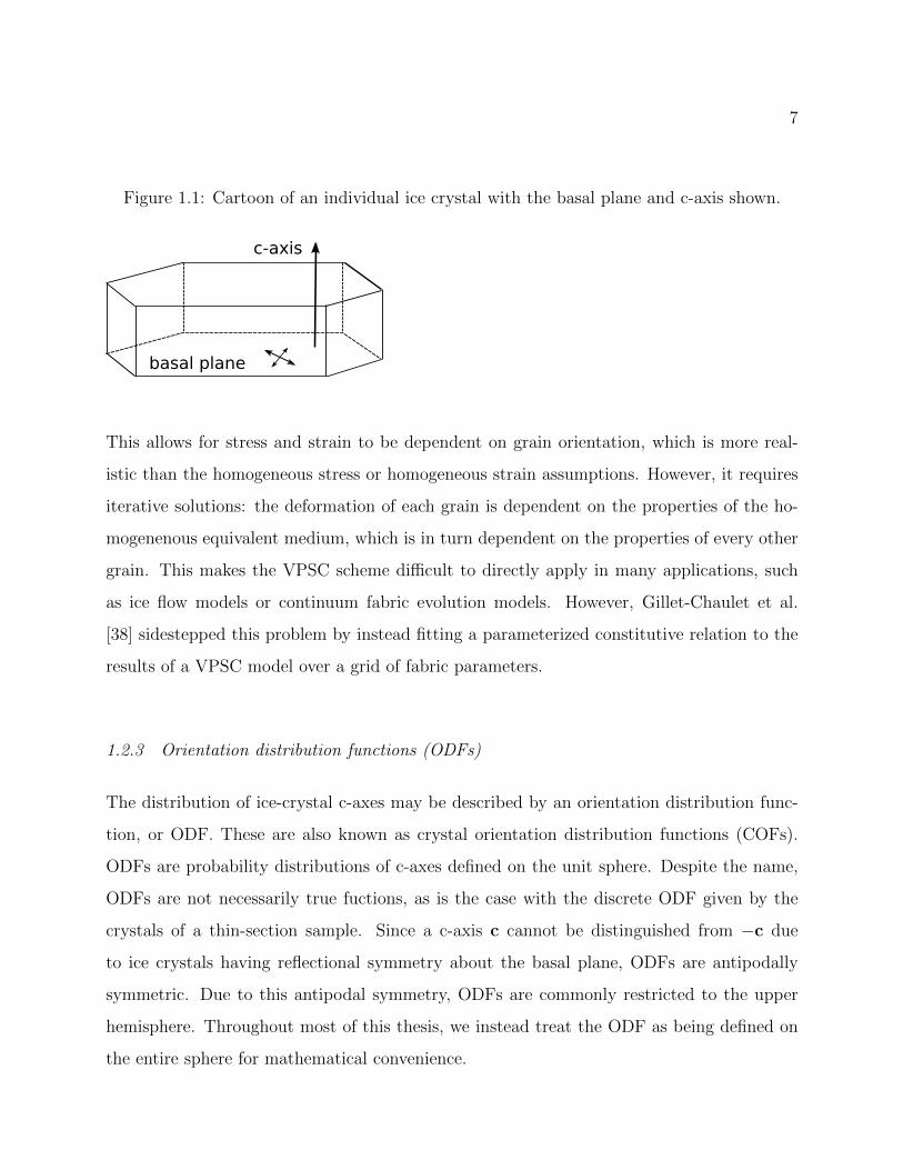
1.1 Cartoon of an individual ice crystal with the basal plane and c-axis shown. . 7
1.2 Schmid plots of thin sections taken from the WAIS divide ice core. Each dotrepresents the c-axis orientation of a single grain. An azimuthal equal-areaprojection is used, such that a grain in the center of the circle is vertical, anda grain on the edge has a horizontal c-axis. A is an approximately isotropicfabric (λ3 ≈ λ2 ≈ λ1); B is a girdle fabric (λ3 ≈ λ2 � λ1); C is a single-maximum fabric (λ3 � λ2 ≈ λ1). . . . . . . . . . . . . . . . . . . . . . . . . 9
2.1 Log-likelihood of maximum-likelihood fits of the Dinh-Armstrong (Equation2.4), Bingham (Equation 2.3), and Fisherian (Equation 2.1) distributions toWAIS and Siple Dome thin-sections. Higher log-likelihood indicates a bet-ter fit. The likelihoods are normalized by grain area for WAIS. For SipleDome, they are normalized by the number of grains. The Dinh-Armstrongand Bingham distributions perform similarly, with the Lliboutry’s Fisheriandistribution having lower likelihood for almost all thin sections. . . . . . . . 24
2.2 Estimates of the diagonal elements Aii (no sum) of the second-order orienta-tion tensor Aij from fabric thin sections from the WAIS Divide core. The errorbars are the 95% bootstrap confidence intervals of the observed area-weightedthin section Aii. . . . . . . . . . . . . . . . . . . . . . . . . . . . . . . . . . . 30
2.3 Bootstrap resampling and analytical estimates of the sample distributions ofthe eigenvalues of the thin section fabric at 140m. The analytical (dashedlines) and resampled bootstrap estimates (solid lines) match closely. Becausethe fabric is rather weak, there is still a moderate amount of uncertaintydespite this sample having 1405 grains. . . . . . . . . . . . . . . . . . . . . . 31
2.4 Bootstrap resampling and analytical estimates of the sample distributionsof the error in fabric Euler angles of the thin section fabric at 140m. Theanalytical and resampled bootstrap estimates match closely. The smallesteigenvalue has a wide distribution in the associated Euler angle, because theother two eigenvalues are close. . . . . . . . . . . . . . . . . . . . . . . . . . 32
iii

2.5 Bootstrap 95% confidence intervals for enhancement factor for the 83 WAISthin sections. Due to the dependence on the fourth power of the averageSchmid factor, the confidence intervals are wide. . . . . . . . . . . . . . . . . 33
3.1 Application of the statistical model to synthetically generated fabric. Thin-section eigenvalues with 30m spacing are generated by adding noise to thetrue eigenvalues. The modeled eigenvalues are close to the true eigenvaluesover the majority of the depth. Error is primarily due to error in the velocity-correction term. . . . . . . . . . . . . . . . . . . . . . . . . . . . . . . . . . . 48
3.2 Velocity corruption (dashed) and estimated velocity corrections (solid lines)for vp, vsh, and vsv. Estimation of the velocity corruption depends on thethin-section eigenvalues. Due to the large degree of spatial variability of thefabric, and the noise in the thin sections, inaccuracies on the order of 10m/soccur. More thin-section samples, and more accurate samples, can reduce thiserror substantially. . . . . . . . . . . . . . . . . . . . . . . . . . . . . . . . . 50
3.3 P-wave velocities modeled from thin sections (dots) and observed P-wave ve-locities (line). The observed P-wave velocities are smoothed over 3m and areaveraged over multiple runs. Due to a combination of model error and veloc-ity drift, the observed velocities are on the order of 100m s−1 less than themodeled velocities. . . . . . . . . . . . . . . . . . . . . . . . . . . . . . . . . 52
3.4 Eigenvalues derived from thin sections at NEEM (dots) [61], together withspatially-continuous estimates from the assimilation procedure. The variabil-ity of eigenvalues over shorter length scales in the upper core appears to bedue to sampling error. The large variations seen in the thin sections in thedeep ice are confirmed by the sonic velocity data. . . . . . . . . . . . . . . . 53
4.1 The six unique components of A for 3000 realizations of the Jeffery’s-typeequation (5.7) forced with pure shear and a strain perturbation whose compo-nents average 2% of the background pure shear, and γ = 1. The central 95%of realizations are shaded. Significant deviations of A13 and A23 occur. Thesecorrespond to tilted cone fabrics whose direction of greatest concentrationdiffers on the order of 5◦ from vertical. . . . . . . . . . . . . . . . . . . . . . 59
4.2 The six unique components of A for 3000 realizations of the Jeffery’s-typeequation (5.7) forced with pure shear and a strain perturbation whose compo-nents average 5% of the background pure shear, with γ = 1. the central 95%of realizations are shaded. Larger deviations of A13 and A23 occur than under2% average perturbations. These correspond to tilted cone fabrics tilted onthe order of 10◦ from vertical. The background pure shear is very effective atrestraining perturbations of other components of A. . . . . . . . . . . . . . . 64
iv

4.3 The six unique components of A for 3000 realizations of the Jeffery’s-typeequation (5.7) forced with simple shear and a strain perturbation whose com-ponents average 2% of the background pure shear, with γ = 1. The central95% of realizations are shaded. Smaller perturbations develop than with pureshear. However, they still may be enough to seed further fabric and flowdisturbances. . . . . . . . . . . . . . . . . . . . . . . . . . . . . . . . . . . . 66
4.4 The six unique components of A for 3000 realizations of the Jeffery’s-typeequation (5.7) forced with simple shear and a strain perturbation whose com-ponents average 5% of the background pure shear, using γ = 1. The central95% of realizations are shaded. Large deviations in A13 and A23 occur thanwith 2% average velocity-gradient perturbations, corresponding to tilted conefabrics deviating on the order of 5◦ from vertical. Smaller deviations occur inother components. . . . . . . . . . . . . . . . . . . . . . . . . . . . . . . . . 68
5.1 Cartoon of the form of a sinusoidal perturbation in space with spatial wavevec-tor κ. The shading represents the sign and magnitude of cos(κ ·x), for a per-turbation of the form v cos(κ ·x), where v is the Fourier coefficient of the per-turbation. The sinusoidal perturbation extends throughout three-dimensionalspace. The plane of the perturbation is given by the plane which is normal tothe wavevector. In this diagram, the positive x-axis extends outwards fromthe page. . . . . . . . . . . . . . . . . . . . . . . . . . . . . . . . . . . . . . . 80
5.2 The largest real part of the eigenvalues of the Jacobian matrix (5.27) undersimple shear, as a function of the largest fabric eigenvalue λ3. Each curve is aperturbation whose wavevector has been rotated by a different angle φ aboutthe y-axis. . . . . . . . . . . . . . . . . . . . . . . . . . . . . . . . . . . . . . 85
5.3 The largest real part of the eigenvalues of the Jacobian matrix (5.27) underpure shear, as a function of the largest fabric eigenvalue λ3. Each curve is aperturbation whose wavevector has been rotated by a different angle θ aboutthe x-axis. . . . . . . . . . . . . . . . . . . . . . . . . . . . . . . . . . . . . . 85
5.4 The largest real part of the eigenvalues of the Jacobian matrix (5.27) underpure shear, as a function of the largest fabric eigenvalue λ3. Each curve is aperturbation whose wavevector has been rotated by a different angle φ aboutthe y-axis. . . . . . . . . . . . . . . . . . . . . . . . . . . . . . . . . . . . . . 86
v

DEDICATION
This thesis is dedicated to my dog Eli.
Outside of a dog, a book is a man’s best friend. Inside of a dog, it’s too dark to read.
- Groucho Marx
vi

ACKNOWLEDGMENTS
This thesis, and my Ph.D. studies have only been possible due to the amazing help and
support I have had from people around me. First and foremost, Ed Waddington has been
the best advisor any grad student could hope for. His support and insight have been integral
to my success.
Thanks also to the rest of my committee. Twit Conway has been a great co-advisor. The
work on Beardmore glacier is a highlight of my Ph.D. Gerard Roe has greatly improved this
thesis with his critical eye on my work. Also, thanks to Randy LeVeque for serving as my
GSR.
My fellow grad students, and my officemates in particular, have been a great source of
support, scientific and otherwise. Thanks to Dan Kluskiewicz, Rob Sheerer, Trevor Thomas,
Adam Campbell, Max Stevens, Elena Amador, John Christian, Taryn Black, and everyone
else.
Thanks also to faculty and postdocs T.J. Fudge, Michelle Koutnik, Al Rasmussen,
Clement Miege.
A big thanks to ESS staff. Thanks to Ed Mulligan for computer support, and Noell
Bernard for her help advising me.
Lastly, thanks to my partner Nick, my parents, and my brother Tom. You don’t choose
your family, but I couldn’t have chosen a better one.
vii

GLOSSARY
ICE CRYSTAL: A region of ice where the crystallographic structure is sufficiently uniformlyoriented.
GRAIN: Synonym for ice crystal.
BASAL PLANE: Crystallographic plane in ice with easy shear.
C-AXIS: Direction orthogonal to the basal plane.
POLYCRYSTAL: A multicrystalline aggregate.
ORIENTATION DISTRIBUTION FUNCTION: Probability distribution of c-axis orientationsof a polycrystal.
SECOND-ORDER ORIENTATION TENSOR: Second moment Aij =< cicj > of an ODF.
FABRIC EIGENVALUE: An eigenvalue of Aij.
HOMOGENIZATION SCHEME: A method of reconciling bulk stress and strain of a poly-crystal to stress and strain of individual grains.
POLYGONIZATION: Splitting of ice grains due to progressive rotation of subgrains.
DYNAMIC RECRYSTALLIZATION: The nucleation and growth of new grains.
ICE DIVIDE: A point where ice flows from in different directions, similarly to hydrographicdivides.
FLANK FLOW: Flow of ice on ice-sheet flanks, away from ice divides. Surface slope pro-vides the driving stress. Movement is mainly due to simple shear, concentrated in thelower layers.
DIVIDE FLOW: Flow of ice near ice divides. Dominated by longitudinal extension.
viii

GAUSSIAN PROCESS: A random function where finite samples of the function follow amultivariate Gaussian distribution.
ix
1
Chapter 1
INTRODUCTION
1.1 Introduction
Individual ice crystals have an unusual amount of plastic anisotropy, with deformation by
shear along the basal plane being around 100 times easier than strain in other orientations
(e.g. Duval et al. [28]). Due to this, the aggregate orientations of crystals (the crystal fabric)
has a large effect on bulk ice flow in ice sheets. If the orientations are anisotropic, the ice
has a bulk anisotropic response to stress. Conversely, ice flow drives development of crystal
orientation fabric in ice sheets.
Aside from understanding ice rheology, ice fabric may be useful itself for paleoclimate
interpretation. Kennedy et al. [49] found that initial differences in fabric at snow deposition
can persist deep into ice sheets. In the NEEM core in Greenland, there is an abrupt change
in fabric corresponding to the Holocene transition [60].
Anisotropic ice flow due to anisotropic crystal fabric can itself hinder paleoclimate inter-
pretation by causing stratigraphic disruption, where isochronous layers can become folded or
removed. Alley et al. [7] found recumbent z-folds in the GISP2 core associated with “stripes”
of anomalously oriented grains. Fudge et al. [32] found evidence of small-scale boudinage
about 750m above the bed in the WAIS divide core. These features may be due to anisotropic
flow.
This thesis is not primarily focused on the detailed microstructural physics of ice, nor is
it directly focused on empirical observations of ice crystal orientation fabrics. Instead, it is
focused on answering the question of what we do not know about ice fabric and anisotropic
ice flow. I explore uncertainties in fabric measurement methods, and also how these un-

2
certainties may be reduced. I examine the effects of velocity-gradient perturbations on ice
fabric. In addition, I study perturbations to fabric as part of a coupled system, and show
that stratigraphic disturbances could occur due to initial fabric perturbations in coupled ice
flow and fabric development.
1.2 Background
In this section, I will give a brief overview of the background material related to this thesis.
I first discuss small-scale ice physics. I review homogenization methods to derive continuum
approximations to polycrystalline ice, as well as fabric evolution.
1.2.1 Ice crystal deformation, rotation, and growth
A cartoon of an individual ice crystal is shown in Fig. 1.1, with the crystallographic c-axis
labeled. An individual ice crystal deforms primarily by dislocation creep in glacial settings
[81]. A dislocation is a defect in the crystal lattice. Since the regular atomic structure of the
crystal is distorted by the dislocation, there is an associated strain and stress field. For edge
dislocations, this takes the form of a dipole, with one pole being compressive and the other
tensile. If an external stress is applied to the crystal, this produces a net driving force on the
dislocation, which can induce the dislocation to move if sufficient stress is realized. When
a dislocation reaches a grain boundary, the crystal is sheared. Dislocations are generated
during strain. As grains become highly strained, dislocations begin to interfere, causing
deformation to become more difficult. This is known as work-hardening, in common with the
metallurgical definition. Dislocations may be removed through the process of recovery, where
dislocations move to minimize their free energy. This occurs partly through the annihilation
of dislocations of opposite sign, and arrangement of dislocations into subgrain boundaries or
to the grain boundaries themselves. The combined effects of dislocation generation, recovery,
and work hardening produces a steady-state density of dislocations at higher strains, and a
steady-state strain rate for constant stress. This steady state is known as secondary creep
[81].

3
The direction of movement of a dislocation is the Burgers vector, denoted by bi. We will
denote the normal to the slip plane by mi. A slip system is the same Burgers vector and slip
plane normal, repeated over the crystal structure. Slip systems are defined by the Schmid
tensor, Eij = bimj. The resolved shear stress on each slip system is given by,
τs = EijSij (1.1)
where Sij is the deviatoric stress experienced by the crystal. The rate of shearing γ on the
slip system is given by the following relation,
γ = B|τn−1s |τs exp
(− Q
RT
)(1.2)
Here, B is a constant, Q is the activation energy of the slip system, R is the universal gas
constant, and T is the temperature. The exponent n is roughly 3 for steady-state dislocation
creep in ice [81], which is the regime glacial ice is usually in.
In ice, easy slip only occurs on the basal plane, where the normal to the plane mi is
given by the c-axis ci. Slip in either prismatic or pyramidal planes is on the order of 100
times harder [28]. This is the mechanism behind the extreme level of plastic anisotropy of
ice compared to most other materials.
Other deformation mechanisms besides basal dislocation slip are usually active in de-
forming ice. Dislocation glide on the basal plane provides two independent slip systems
(corresponding to the two degrees of freedom of the plane). However, a minimum of five
independent slip systems is needed to accomodate arbitrary deformations [80]. During de-
formation, grains well-oriented towards basal slip will begin to deform, but are blocked by
hard-oriented grains. The resulting stress may be relieved through several mechanisms.
Grain boundary sliding can occur to maintain compatibility between adjacent grains. Non-
uniform deformation involving bending of the lattice may occur within grains. This can
result in the formation of subgrain boundaries [65]. In addition, slip along prismatic planes
may occur in some circumstances [65].
The most commonly used constitutive relation for isotropic ice is Glen’s flow law [39],

4
which is closely related to Eq. (1.2):
Dij = BSijτn−1e exp
(− Q
RT
), (1.3)
where τe is the effective stress, and Dij is the strain-rate tensor. The exponent n is usually
set to 3, in common with the exponent for steady-state dislocation creep.
To maintain compatibility with other grains (and the externally applied strain), lattice
rotation occurs during dislocation creep. This induces c-axes to rotate towards directions
of principal compression. For example, in vertical compression prominent near ice divides,
c-axes rotate towards vertical. This makes the ice harder under applied vertical compression,
since there is is a smaller component of shear stress along the basal plane. In the extreme
case where a grain pointed exactly vertically is subjected to vertical compression, there is
no resolved shear stress on the basal plane. Thus, the crystal does not deform through basal
glide at all.
In the case where deformation occurs solely due to slip on the basal plane, the rate of
c-axis rotation due to lattice rotation is given by a modified Jeffery’s equation [58],
ci = Vijcj −Dgijcj + cicjckD
gjk. (1.4)
Here Vij is the bulk vorticity tensor, corresponding to externally applied spin. The quantity
Dgij is a component of the strain-rate tensor experienced by the grain (rather than the global
strain rate). The last term of Equation (1.4) ensures that the rotation of the c-axis is tangent
to the sphere, to maintain unit length. This can be seen by noting that the Vijcj term does
not affect the magnitude of ci, leaving only the Dijcj term. Assume that at time t = 0, the
c-axis is given by c0. After a short length of time δt, the magnitude of the new c-axis cδt is
(without the final term in Equation 1.4),
||cδt|| = ||c0 − δtDc|| (1.5)
≈ ||c0||−cT0Dc0δt (1.6)
= 1− cT0Dc0δt, (1.7)

5
to first order in δt. Thus, for the c-axis to maintain unit length, we must add the quantity
cTDcδt projected onto c, by multiplying by c. This then gives the last term of Equation
(1.4).
While deformation-induced grain rotation is the most important process governing fabric
development in ice sheets, other processes play a role in both fabric development and ice
rheology. There is evidence that grain size plays a significant role in ice deformation. Cuffey
et al. [18] used observations from the Meserve Glacier in Antarctica to argue that grain-size
variations explain a significant amount of enhanced shear in ice-age ice in Greenland.
Grain growth, in which some grains grow at the expense of others, occurs throughout ice
sheets. Normal grain growth is most prominent in upper layers of ice sheets, where grains
are not yet highly strained. Here, large grains grow at the expense of small grains due to
differences of curvature. Grain boundaries with high curvatures have more unmade bonds
per unit area; these unmade bonds possess free energy. Smaller grains have higher positive
curvature over more of their boundary than large grains, making it energetically favorable
for large grains to consume small ones [59].
As grains become more highly strained, the process of polygonization (also known as
rotation recrystallization) works against normal grain growth. As noted previously, bending
of the crystal lattice induces the formation of subgrain boundaries, because dislocations
lying in different basal planes can minimize their strain energy fields by lining up. As this
process continues, and the subgrain misorientation increases, the subgrains become distinct
grains. This process also reduces the work-hardening of grains, since dislocations are moved
from grain interiors to the new grain boundaries. Polygonization causes changes in grain
orientation of no more than a few degrees [6]. It does not significantly change the resolved
shear stress of the resulting child grains.
In contrast to polygonization, dynamic recrystallization (also known as migration recrys-
tallization or discontinuous recrystallization) can greatly change grain orientations. Highly
strained grains have a high dislocation density, which carries a great amount of strain energy.
Newly nucleated grains with low dislocation densities can then easily grow, with the reduc-

6
tion in dislocation density providing the main driving force. These grains are typically well
oriented for basal glide. Dynamic recrystallization typically occurs in waves, as new grains
rapidly grow and consume the older, more strained grains (e.g. Montagnat and Duval [59]).
This produces an interlocking texture of irregular, very large (up to several cm3) grains. This
provides an important mechanism to control the strength of ice fabrics deep in ice cores. In
particular, near ice divides, it limits the tendency of c-axes to line up to vertical under the
applied vertical compression. This limits the hardness of the ice under the applied stress.
Dynamic recrystallization is usually active only above about −10◦C, which occurs in deeper
layers in most ice-sheet locations. Although, dynamic recrystallization is evident in layers
as shallow as 200m at Siple Dome at temperatures of around −20◦C [21].
1.2.2 Homogenization
A key difficulty of any continuum treatment of anisotropic ice is stress and strain homoge-
nization: Stress and strain of individual grains must be consistent with the global stress and
strain of the entire polycrystal. The homogenization scheme must also be tractable. There
are two possible end-members. First, the Taylor-Bishop-Hill model [74] assumes homoge-
neous strain among grains, while allowing stress between grains to vary so as to produce
the required global strain. This method is well-suited to materials with several active slip
systems. It also has the advantage of avoiding overlap between grains: because every grain
has the same strain, compatibility is guaranteed. An alternative approach is the Sachs model
[69], which assumes homogeneous stress among grains. The strain of each grain is such that
the global stress is maintained. This model does not produce strain compatibility, which can
produce nonphysical overlaps between grains. Nonetheless, it produces better bulk strain
and stress predictions for ice than the homogeneous strain model, because ice typically has
only two active slip systems.
In the middle between these two are visco-plastic self-consistent (VPSC) schemes [52].
Here, each individual grain is treated as an ellipsoidal inclusion in an infinite, homogeneous
matrix with the average properties of the polycrystal (the homogeneous equivalent medium).
7
Figure 1.1: Cartoon of an individual ice crystal with the basal plane and c-axis shown.
basal plane
c-axis
This allows for stress and strain to be dependent on grain orientation, which is more real-
istic than the homogeneous stress or homogeneous strain assumptions. However, it requires
iterative solutions: the deformation of each grain is dependent on the properties of the ho-
mogenenous equivalent medium, which is in turn dependent on the properties of every other
grain. This makes the VPSC scheme difficult to directly apply in many applications, such
as ice flow models or continuum fabric evolution models. However, Gillet-Chaulet et al.
[38] sidestepped this problem by instead fitting a parameterized constitutive relation to the
results of a VPSC model over a grid of fabric parameters.
1.2.3 Orientation distribution functions (ODFs)
The distribution of ice-crystal c-axes may be described by an orientation distribution func-
tion, or ODF. These are also known as crystal orientation distribution functions (COFs).
ODFs are probability distributions of c-axes defined on the unit sphere. Despite the name,
ODFs are not necessarily true fuctions, as is the case with the discrete ODF given by the
crystals of a thin-section sample. Since a c-axis c cannot be distinguished from −c due
to ice crystals having reflectional symmetry about the basal plane, ODFs are antipodally
symmetric. Due to this antipodal symmetry, ODFs are commonly restricted to the upper
hemisphere. Throughout most of this thesis, we instead treat the ODF as being defined on
the entire sphere for mathematical convenience.

8
Orientation tensors
Orientation distribution functions are often summarized using symmetric orientation (or,
moment) tensors [2]. These tensors are used throughout this thesis. The element with index
i1, ..., in of the nth order orientation tensor Ti1,..,in is given by the outer product of of the
c-axis with itself, n times, averaged over the ODF,
Ti1,..,in =<n∏j=1
cij > . (1.8)
Since ODFs are antipodally symmetric, odd-order tensors are zero. Usually the fabric is
described with only the second-order orientation tensor Aij =< cicj >. This is a symmetric,
3 × 3 tensor. The second-order orientation tensor is also the covariance tensor of the ODF
if it is viewed as a distribution in Cartesian space with support confined to the sphere. The
definition of covariance of a distribution is the second moment about the mean, given by,
Cov(ci, cj) =< (ci− < ci >)(cj− < cj >) > (1.9)
Since the mean (or first-order orientation tensor) < ci > is zero due to antipodal symmetry,
this reduces to Aij =< cicj >.
Because it is symmetric, there exists a reference frame where Aij is diagonal with eigen-
values λ1 ≤ λ2 ≤ λ3 which sum to unity. They sum to unity by construction because all
c-axes lie on the unit sphere. The corresponding eigenvectors are also known as fabric prin-
cipal directions. The eigenvalues correspond to concentrations of fabric in each principal
direction. The principal direction associated with the largest eigenvalue λ3 has the high-
est concentration of c-axes, and the principal direction association with λ1 has the lowest
concentration. The eigenvalue λ2 is associated with the direction orthogonal to the other
two.
If λ3 ≈ λ2 ≈ λ1, then the fabric is isotropic, with c-axes distributed nearly uniformly
across the sphere. If instead λ3 � λ2 ≈ λ1, then the fabric is known as a single-maximum,
or pole fabric. In the case where λ3 ≈ λ2 � λ1, then the fabric is a girdle fabric, with a

9
Figure 1.2: Schmid plots of thin sections taken from the WAIS divide ice core. Each dotrepresents the c-axis orientation of a single grain. An azimuthal equal-area projection isused, such that a grain in the center of the circle is vertical, and a grain on the edge has ahorizontal c-axis. A is an approximately isotropic fabric (λ3 ≈ λ2 ≈ λ1); B is a girdle fabric(λ3 ≈ λ2 � λ1); C is a single-maximum fabric (λ3 � λ2 ≈ λ1).
A B C
concentration of c-axes lying near the great circle orthogonal to λ1. Examples of each of
these fabric types from the West Antarctic Ice Sheet (WAIS) divide ice-core [30] are shown
in Figure 1.2.
The fourth-order orientation tensor Aijkl =< cicjckcl > is also necessary for many flow
and fabric evolution calculations. While it is not typically used to describe ice fabrics,
it can account for more complex fabric types, such as fabrics with multiple maxima. In
practice, this is usually estimated from the second-order orientation tensor through closure
approximations (see next section).
Zheng and Zou [84] showed that an ODF may be expressed as as an expansion of orthog-
onal traceless basis-functions, with coefficients derived from orientation tensors. The first
two terms of this expansion are given by,
ψ(c) =1
4π+
15
2
(Aij −
1
3δijcicj
)+ ... (1.10)
If we are working in the reference frame defined by the fabric principal directions, such that
the second-order orientation tensor is diagonal, the link between fabric eigenvalues and ODF

10
density can be readily seen. Unfortunately, this series expansion approach is not usually
useful to describe most fabrics. If the expansion is truncated at the second-order, as above,
the second-order orientation tensor of the truncated distribution is not necessarily the same
Aij it is parameterized by (i.e., Aij on the right-hand side of Eq. 1.10). In particular, the
second and fourth-order trunctions cannot represent very strong single-maximum fabrics.
Basis functions and coefficients beyond the fourth order have unfeasibly many terms.
1.2.4 Continuum fabric evolution models
Eq. (1.4) gives the rotation rate of a single grain. When modeling bulk fabric, it is not
practical to treat each grain individually. Instead, we may derive an evolution equation for
the second-order orientation tensor Aij. This has only six unique components, reducing an
expensive computational problem to a small ODE system. Suppose that we have an ODF
ψ(c) giving the density of c-axes at c.
dAijdt
=< cicj > + < cicj > . (1.11)
Replacing c in the above equation with Eq. (1.4), we arrive at the following evolution
equation for the material derivative of Aij:
dAijdt
= VikAkj − AikVkj −DikAkj − AikDkj + 2AijklDkl. (1.12)
The last term involves the fourth-order orientation tensor Aijkl, which introduces the closure
problem: to determine the evolution of the second-order orientation tensor, we need the
fourth-order orientation tensor. We could similarly use an evolution equation for the fourth-
order orientation tensor, but the sixth-order orientation tensor would appear in that equation,
and so on. Thus, we need some way to approximate the fourth-order tensor Aijkl in terms
of Aij. In the fiber literature, a vast array of closure approximations have been proposed to
solve this problem. I will discuss a few here.
Perhaps the simplest is the quadratic closure, where Aijkl = AijAkl. This is exact in
the case of perfectly concentrated fabrics, where λ3 = 1. It is quite accurate whenever

11
λ3 > 0.8, and produces reasonably accurate predictions for the c-axis rotation rate even for
diffuse fabrics. The quadratic closure is still the most common closure used for industrial
fiber-orientation models due to its simplicity and reasonable accuracy.
Another simple closure is the linear closure,
Aijkl = − 1
35(δijδij + δijδij + δijδij)
+1
7(Aijδkl + Aikδjl + Ailδjk + Aklδij + Ajlδik + Ajkδil). (1.13)
The linear closure is exact for isotropic fabrics, but produces invalid predictions for strong
single-maximum fabrics. Therefore, it is not a good choice itself as a closure approximation
in ice, because strong single-maximum fabrics are common in deeper layers of ice sheets.
The hybrid closure [3] instead takes a weighted average of the linear and quadratic closures,
where the weighting is usually dependent on the largest eigenvalue λ3. This can exactly
represent both isotropic fabrics and perfect single-maximum fabrics.
Other, more sophisticated closures exist. Chung and Kwon [16] proposed the invariant-
based orthotropic fitted (IBOF) closure. This closure writes Aijkl using polynomial functions
of the invariants of Aij. The coefficients of the polynomial functions are fitted to a particular
assumption of the form of the ODF, or to empirical data. This closure approximation was
used by Gillet-Chaulet et al. [38] by fitting to an analytical distribution.
Lastly, I examine the fast exact closure [63]. If a fabric is initially isotropic, and evolves
only due to lattice rotation from basal slip, then the ODF has the following form:
φ(c) =1
4π(cTBc)3/2(1.14)
where B = CTC has a determinant of unity and C follows the equation,
dC
dt= −C(D + W) (1.15)
Rather than solving the Jeffery’s equation (1.12) directly, only the previous ODE (1.15)
must be integrated. This sidesteps the closure problem entirely. The orientation tensors
Aij and Aijkl can be easily recovered using Carlson symmetric integrals. However, it is not
12
necessary to compute Aijkl in order to integrate the evolution of the fabric through time.
This closure is not exact in the case of ice fabrics, since they typically are not initially
isotropic, and do not follow the distribution given by Eq. (1.14) exactly. However, I have
found that this distribution does an excellent job of approximately fitting thin-section data.
This suggests that this closure approximation would be accurate in practice for predicting
ice fabric development. The IBOF closure used by Gillet-Chaulet et al. [38] is in fact a
polynomial approximation to this closure. Compared to the IBOF closure, the fast exact
closure has a simpler implementation and better theoretical motivation. In addition, it is
also more computationally efficient if Aij and Aijkl do not need to be computed at every
timestep.
1.3 Outline
This thesis is divided into four main chapters, corresponding to four manuscripts. In the
second chapter, I examine statistics and sampling error in ice-core thin sections. I derive
novel estimates of sampling error in fabric, and apply these estimates to thin-section data
from the WAIS divide ice-core [30]. I show that thin-section sampling error can be large
under area-weighted thin sections. I also introduce a new parameterized ODF to glaciology,
and compare the fits of this and other distributions in the WAIS and Siple Dome ice cores.
The last two main chapters examine the sensitivity of anisotropic flow to perturbations of
flow and fabric. In the fourth chapter, I examine the sensitivity of ice fabrics to velocity gra-
dient perturbations. I show that small velocity-gradient perturbations can induce tilted-cone
fabrics in simple shear and pure shear, where the direction of greatest c-axis concentration
is not vertical. These fabrics can induce vertical motion in horizontal simple shear.
The fifth chapter is an expansion on the third: given that small velocity perturbations
can cause significant fabric perturbations, can the dynamics of coupled ice flow and fabric
evolution cause these perturbations to grow further? I examine this by developing an ana-
lytical first-order model of coupled anisotropic ice flow and fabric perturbations. I show that
under pure shear and simple shear, fabric perturbations in single-maximum fabrics can be

13
unstable.
The contributions of this thesis are significant in several ways. I provide a thorough
examination of methods of measuring crystal orientation fabrics in boreholes. The rigorous
estimates of thin-section sampling error I developed are generally larger, and more realistic
than previous estimates. Accurate estimates of uncertainties will aid usage of fabric data
for paleoclimate interpretation. In addition, my uncertainty estimates may also be useful
to inform thin-section sampling done in future ice cores. Finding the best number and the
best locations of thin-section samples for an ice core is a trade-off between consumption of
limited core ice, labor, accuracy, and spatial coverage. By providing accurate estimates of
uncertainty based on grain-size distributions and fabric eigenvalues, these decisions can be
better justified.
Inference of fabric using sonic velocities and thin-section measurements is a promising
technique to combat sampling error or bias in sonic measurements, and sampling error in
thin sections. Borehole sonic logging has received increased interest over the past several
years. Given that thin-section measurements usually taken from ice cores anyway, this
technique can improve accuracy with little cost. My statistical approach to fabric inversion
also makes fewer assumptions on the form of the ODF compared to previous work. It is
also an innovative use of the Google Tensorflow machine learning library for a geophysical
inversion problem. This has the potential to be a convenient tool to use in other, similar
problems.
The last two chapters of this thesis provide the most comprehensive examination of stabil-
ity of ice-crystal fabrics to date. Stratigraphic disruption due to anisotropy has received little
attention, despite being the most plausible cause of smaller-scale stratigraphic disturbances
seen off the bed. In addition, anisotropy probably plays a strong role in large-scale folding
and stratigraphic disruption in basal ice, due to its ability to create very large differences in
viscosity. The work in this thesis is a start to understanding this complicated topic.
14
Chapter 2
STATISTICAL ASPECTS OF ICE-CRYSTAL ORIENTATIONFABRICS
This chapter is in review at the Journal of Glaciology, with Ed Waddington as co-author.
I developed the statistical results and wrote this manuscript. Ed Waddington helped edit
the manuscript and contributed useful discussions.
Abstract: Ice crystal orientation fabric has a large effect on polycrystalline ice flow due
to the strong plastic anisotropy of individual grains. The crystal orientation fabric can be
described as an orientation distribution function (ODF), which is a probability distribution
defined on the sphere for the direction of crystal c-axes. From this viewpoint, we present
several statistical results for ODFs. We introduce a parameterized ODF (PODF), the Bing-
ham distribution, to glaciology. We compare the performance of this and other PODFs
against measurements from the West Antarctic Ice Sheet (WAIS) and Siple Dome ice cores.
We also examine the sampling error introduced by attempting to infer the larger-scale bulk
ODF from a thin-section sample. We introduce new analytical expressions for sampling er-
ror, and examine the use of bootstrapping for estimation of sampling error. We show that
sampling error of fabric parameters can be substantial. Finally, we examine sampling error
from inferring enhancement factor in Glen’s flow law from thin sections. We show that rhe-
ological properties of ice are very poorly constrained by thin-section measurements, due to
the power-law constitutive relation of ice in the dislocation-creep regime.
2.1 Introduction
An individual ice crystal has an anisotropic creep response, deforming most easily in shear
parallel to the crystal basal-plane, orthogonal to the crystallographic c-axis. Plastic deforma-
15
tion of an ice polycrystal depends on the orientations of its constituent grains (e.g. Azuma
[8]), which is described by the c-axis orientation distribution function (ODF). The ODF is
a probability distribution of c-axis density often defined on the upper hemisphere (because
a c-axis vector c is indistinguishable from −c). In this paper, we will instead treat the
ODF as being an even function defined on the entire sphere for mathematical convenience.
A polycrystal with an isotropic ODF will have a bulk isotropic response to applied stress.
However, polycrystals develop an anisotropic ODF in response to applied strain.
The development of a preferred orientation is guided primarily by intracrystalline slip.
Due to interference among grains, there is a tendency for the c-axes to rotate away from the
directions of principal extensional strain [10]. ODFs are often summarized using orientation
(or, moment) tensors (e.g. Svendsem and Hutter [73]). We will make extensive use of index
notation in this paper, due to the use of higher-order tensors. However, at times we will not
follow the summation convention for notational convenience (this is noted when it occurs).
In addition, throughout this paper, indices 1, 2, and 3 are associated with the x, y, and z
directions, respectively. The second-order orientation tensor Aij is the expectation < cicj >,
where i, j = 1, 2, 3. The mean of the ODF, < ci >, is always zero because of antipodal
symmetry. Therefore, Aij is also the covariance matrix of the distribution, by definition of
covariance as Cov(ci, cj) =< (ci− < ci >)(cj− < cj >) >. The diagonal elements A11, A22,
and A33 give a measure of the c-axis concentration on the x, y, and z axes, respectively.
Similar to the second-order orientation tensor, the fourth-order tensor is the expected value
Aijkl =< cicjckcl >. Since ODFs over the sphere are antipodally symmetric, odd-order
tensors are zero. The symmetric second-order orientation tensor may be decomposed into
non-negative eigenvalues and three orthogonal eigenvectors. The eigenvalues of A sum to
unity by construction. The eigenvectors, or fabric principal directions, denote the directions
of greatest density (corresponding to the largest eigenvalue), smallest density (the smallest
eigenvalue), and a direction orthogonal to the other two. An isotropic fabric has three equal
eigenvalues. A girdle fabric (in which there is a band of high concentration along a great
circle) has two nearly equal eigenvalues, and one small eigenvalue. A single-maximum fabric

16
Table 2.1: List of symbols
Symbol Definition
qi Component of a tensor in index notation
q Same tensor in vector notation
x Sample estimate of a quantity x
ci ice-crystal c-axis for i = 1, 2, 3 in x, y, z directions
ψ(c) Ice-crystal orientation dist. func.
< qi > Expected value of qi under ψ
aij Grain structure-tensor cicj
Aij Comp. of the 2th order orient. tensor < aij >
Aijkl Comp. of the 4th order orient. tensor < aijakl >
λi Fabric eigenvalue of A
V Matrix of eigenvectors of A
φ Zenith angle
θ Azimuth angle
δij Kronecker delta symbol
S2 Unit sphere
σ A standard deviation
Sij Stress tensor
B Bingham distribution (Equation 2.3)
L Diagonal concentration matrix of BD Dinh-Armstrong distribution (Equation 2.4)
R Parameter matrix of DF Lliboutry’s Fisherian distribution (Equation 2.1)
W Watson distribution (Equation 2.2)
κ Scalar concentration parameter for Fη Scalar concentration parameter for W

17
has one large eigenvalue, and two small ones. Small-girdle fabrics can also occur during
active recrystallization, where a small ring of high density exists around the axis-preferred
orientation of the applied strain and vorticity (typically centered around vertical).
It is common to approximate the unknown, true ODF with a parametric ODF (PODF),
which can normally be fit to observed fabric data. This reduces the number of parameters.
Among other uses, it is usually necessary to assume a specific PODF to numerically model
fabric evolution. Numerous PODFs have been proposed. The majority have an axis of
rotational symmetry, which is valid for single-maximum fabrics and symmetric girdle fabrics.
Several PODFs have been developed that are motivated by analytical solutions to c-axis
evolution valid in specific flow regimes (e.g. Staroszczyk and Gagliardini [72], Svendsem and
Hutter [73], Gagliardini and Meyssonnier [33], Godert and Hutter [41]). However, Gagliardini
et al. [36] noted that these are special cases of the Dinh-Armstrong distribution [20]. This
is a very flexible distribution that does not assume axial symmetry. Any initially isotropic
fabric which evolves due only to deformation-induced grain rotation has this ODF. Other
distributions have been proposed based on heuristic considerations (e.g. Thorsteinsson [75],
Lliboutry [54]). More recently, Kennedy et al. [49] proposed the axially symmetric Watson
distribution for use as PODF. For a complete overview of this topic, see Gagliardini et al.
[36]. In this paper, we propose the Bingham distribution as an ODF, motivated primarily
by statistical considerations. The Bingham distribution is a generalization of the Watson
distribution.
Sampling error can be significant when inferring bulk properties of ice from a small thin-
section sample. By “bulk properties” we mean those averaged out over large ice volumes.
What constitutes a “larger volume” is somewhat arbitrary, but is at least as large as to render
sampling error insignificant over the length scales of the larger volume. Sampling error is
the error from approximating something (here, the bulk properties of ice) from a limited
sample size. Therefore it is important to take sampling error into account when interpreting
ice-sheet thin sections in order to properly interpret thin-section data. In addition, this
sampling error can also be viewed as variability in the underlying ODF on the scale of thin
18
sections. This can cause variability of anisotropic viscosity on the scale of thin sections.
Thorsteinsson [75] found that around 5000 grains are needed to effectively eliminate
sampling error in a fabric model. Later on, Durand et al. [24] fit a quadratic estimate
of the sampling error of A by generating an array of fabrics of 10,000 grains each, and
resampling from these fabrics. Unfortunately, this method is not directly applicable to
per-pixel measurements, such as with electron backscatter diffraction or automatic fabric
analyzers, since it does not take into account the correlation of nearby measurements.. Here,
we introduce an analytical estimate for the sampling distribution of fabric eigenvalues and
eigenvectors based on data taken from a discrete thin-section sample, with either equal
weighting of grains, or weighting by area. Generally, area weighting should be preferred, as
it more accurately reflects the true fabric by giving a larger weight to larger grains [35].
When fabric eigenvectors and eigenvalues are derived using area weighting of crystals in
thin sections, we show that sampling error can be greatly increased. We also numerically
derive an estimate of the sampling distribution of enhancement factor [53] under simple shear
from thin sections. This random variability for regions of several hundred grains can also
affect small-scale flow. This may be a source of incipient layer folds, which can then be
overturned by anisotropically-enhanced shearing deep in ice sheets [76].
2.2 Parameterized orientation-density functions (PODFs)
We now examine the use of PODFs. We discuss several previously used PODFs which we
consider to be especially statistically and physically plausible. We introduce the Bingham
distribution as a PODF. We then compare the log-likelihoods of the distributions fitted to
thin-section data at the West Antarctic Ice Sheet (WAIS) Divide ice core and the Siple Dome
ice core, to assess their performance.
2.2.1 Fisher and Watson distributions
Lliboutry [54] first suggested the use of an axially-symmetric Von Mises-Fisher type distri-
bution. Expressed in a reference frame where the vertical axis is aligned with the symmetry
19
axis, this is,
F(φ) =κ exp(−κ cos(φ))
eκ − 1, (2.1)
where φ is the zenith angle, and κ is a scalar concentration parameter. Gagliardini et al.
[36] found that this distribution provided the best fit for fabric in a thin section from the
Dome C core. As a modification to the Lliboutry’s Fisherian distribution, Kennedy et al.
[49] introduced the Watson distribution for use as a PODF:
W(φ) = a exp(−η cos2(φ)), (2.2)
where η is a concentration parameter, φ is the zenith angle, and a is a normalization constant.
Note that by the double-angle formula, if the concentration parameters η (for the Watson
distribution) and κ (for the Fisher distribution) are equal, then F(2φ) ∝ W(φ). Both of these
distributions can represent single-maximum fabrics with positive concentration parameters,
and the axis of symmetry parallel to the eigenvector associated with the largest eigenvalue.
Likewise, girdle fabrics can be represented with negative concentration parameters, with the
axis of symmetry parallel to the eigenvector associated with the smallest eigenvalue. The
Watson distribution has the important advantage of being antipodally symmetric. Because
individual ice-crystal orientations cannot be distinguished between c and −c, any ice ODF
defined on the sphere should also be antipodally symmetric. It is common practice to define
ODFs only on the upper hemisphere. Any ODF defined on the upper hemisphere can trivially
be extended to the whole sphere. However, this does not, in general, preserve smoothness
(which is usually desirable). For the Von Mises-Fisher distribution of Lliboutry, the derivative
of density with respect to φ does not vanish at the equator. If we extend this ODF to the
whole sphere, the derivative is discontinuous at the equator. The discontinuity does not have
a physical basis. This same difficulty appears when extending any distribution on the half
to the full sphere whose density gradient does not vanish at the equator.

20
2.2.2 The Bingham Distribution
We now introduce the Bingham distribution [13] as a generalization of the Watson distribu-
tion. The density, in Cartesian coordinates, is
B(c) = γ(L) exp(−cTVLVTc), (2.3)
where V is the matrix of eigenvectors of the second-order orientation tensor A, and γ is
a normalization constant. Also, L is a diagonal matrix containing three concentration pa-
rameters ιi such that ι1 < ι2, ι3. This distribution is invariant for changes in the sum of
concentration parameters, because any change in the sum of concentration parameters is
negated by a change in the normalizing constant γ(L). Because of this, we may set ι1 = 0,
since if the parameters are ιi, with ι1 6= 0, the distribution with concentration parameters
ιi − ι1 is identical. This reduces the number of free parameters from three to two. If we set
ι2 = 0 as well, the Watson distribution (Equation 2.2) is recovered. This distribution has
a number of desirable properties. It is able to represent single-maximum fabric and girdle
fabrics, but is also able to capture fabrics with three distinct eigenvalues, such as oblong
maxima, or girdles that are concentrated in one direction.
In addition, the Bingham distribution is parsimonious. If we seek a PODF with a given A,
then the Bingham distribution avoids introducing spurious structures that are unnecessary
to satisfy the assumption of a particular value of A. Specifically, the Bingham distribution is
the maximum-entropy distribution for any spherical distribution with a given second-order
orientation tensor (or, covariance matrix) [55].
Distributional entropy is defined very similarly to thermodynamic entropy (the latter
can be seen as a special case of the former). The entropy of a probability distribution q
is the expectation < − log q >. Distributions that have high entropy contain less infor-
mation. Higher-entropy distributions are therefore more parsimonious (due to having less
information). Thus, when selecting a parametric distribution, the distribution with the
highest entropy that adequately fits the given data is the most parsimonious explanation of
the observations. Such a distribution fits the data well, but without assuming extraneous

21
information. In this sense, the Bingham distribution is similar to the multivariate normal
distribution, which has maximum entropy of any distribution over n-dimensional Euclidean
space possessing a given covariance matrix, or the exponential distribution, which has the
maximum entropy of any distribution on the line with a given mean. The Bingham distri-
bution is in fact the multivariate normal distribution with zero mean conditioned to lie on
the unit sphere.
The Bingham distribution has found use in paleomagnetics [64] and other fields. How-
ever, its wider adoption has been hampered by a lack of closed-form analytical expressions
for the normalization constant and the maximum-likelihood estimator of ιi given the data,
necessitating a greater use of slower numerical methods than many other distributions. How-
ever, this is not as great of a challenge as it once was. In addition, since the distribution is
determined by two parameters, it is amenable to methods based on lookup tables.
In fitting a Bingham distribution to an observed fabric, only the second moment of the
observed fabric, A, is needed. Higher moments are neglected, which means the Bingham
distribution cannot fit complex fabric distributions, such as those with multiple maxima.
It is possible to derive distributions fitting higher moments. However, this would quickly
become unwieldy. In addition, if the goal is to estimate a bulk fabric distribution from a
limited thin-section sample, more complex distributions would tend to overfit the data.
2.2.3 The Dinh-Armstrong distribution
We now examine another distribution, which we will refer to as the Dinh-Armstrong distri-
bution [20]. This is given by,
D(c) =1
4π (cTRc)32
, (2.4)
where R is a symmetric second-order tensor with a determinant of unity. Gillet-Chaulet
et al. [38] introduced this distribution to glaciology for fabric evolution. If c rotates due only
to slip on the basal plane, and if the ODF was at one time isotropic, then the ODF has this
distribution with R = FFT, where F the bulk deformation gradient. In the reference frame

22
defined by the fabric principal-directions, R is a diagonal matrix, with diagonal entries bi.
The three elements bi possess only two degrees of freedom, due to the constraint that the
determinant is unity.
2.2.4 Comparison of PODFs
We now compare the Dinh-Armstrong distribution (Equation 2.4), the Fisherian distribution
(Equation 2.1), and the Bingham distribution (Equation 2.3) using thin-section data from the
WAIS Divide ice core [30] and the Siple Dome ice core [82]. We found a maximum-likelihood
fit of each of these three distributions for each thin section. The data likelihood of a parameter
value ω of a parameterized distribution fω is the probability of those observed data arising
under the distribution fω (with the parameter value ω). The maximum-likelihood value of ω
is the value of ω that maximizes this likelihood. That is, the maximum-likelihood estimator
maximizes Pr(d|ω), where d is the observed data. In practice, the log-likelihood is maximized
instead of directly maximizing the likelihood. Maximum-likelihood estimation is a standard
way to fit distributions to data for many statistical tasks. It provides a coherent measure
of the fitness of a distribution to data. Thus, comparing log-likelihoods of data for the
maximum likelihood fits of these distributions is a fair way of comparing their performance.
For the Bingham distribution (Equation 2.3), we computed the maximum-likelihood den-
sity estimates of L numerically, given the observed grain orientations from the WAIS and
Siple Dome ice-cores. For the Dinh-Armstrong distribution (Equation 2.4), we numerically
found the maximum-likelihood estimates for the parameter R. For Lliboutry’s Fisherian dis-
tribution with a single-maximum fabric, we first rotated the reference frame into the fabric
principal reference frame such that the eigenvector corresponding to the largest eigenvalue
points vertical. For Lliboutry’s Fisherian distribution with a girdle fabric, we rotated the
reference frame such that the eigenvector associated with the smallest eigenvalue is vertical.
We then numerically found the maximum-likelihood estimates for the concentration parame-
ter κ. The results for all three PODFs, for both WAIS and Siple Dome, are plotted in Figure
2.1.

23
We consider the normalized log-likelihoods of thin-sections (normalized by either thin-
section area or number of grains), rather than the likelihood of observing all grains in each
thin section. Normalized log-likelihood gives the average likelihood of observing a grain from
a thin section. This is necessary because the thin sections differ in the number of grains, so the
likelihoods of each thin section (with all grains taken together) are not directly comparable.
Everything else being equal, a sample with more grains will have lower likelihood than a
sample with few grains. Note that we are plotting the log-likelihood of each distribution,
for the maximum-likelihood values of the parameters L, κ, and R. We are not plotting the
values of these parameters themselves, since they are not comparable between distributions,
and they themselves give no information on the goodness of fit. The Fisherian distribution
has the lowest log-likelihood for nearly all thin sections. The Bingham and Dinh-Armstrong
distributions perform similarly, with the Bingham distribution slightly outperforming the
Dinh-Armstrong distribution overall. For these data as a whole, this indicates that the
Bingham distribution is the best choice due to its maximum-entropy property. However, the
Dinh-Armstrong distribution does not have a normalization constant that must be found
numerically, as the Bingham distribution does. Therefore, it may be a better choice for many
applications. Different physical situations are not likely to be fit by a single ODF. However,
both the Dinh-Armstrong (Equation 2.4) and Bingham (Equation 2.3) distributions have
physical motivation, and may serve as good default PODFs.
All three PODFs are capable of exactly representing isotropic fabrics, and in the limit,
perfect single maximum fabrics. Thus, they perform similarly in the less-anisotropic fabric
near the top of the WAIS divide ice core. Log-likelihoods are usually lower for diffuse fabrics
than for concentrated fabrics. In concentrated fabrics, most of the grains lie in orientation
which have high ODF density, resulting in high likelihoods. In the limit of grains taken from
a perfect single-maximum fabric, the likelihood of each grain is positive infinite. On the
other hand, in the limit of an isotropic fabric, the unnormalized log-likelihood of every grain
is always − log(4π). This is because the area of the surface of the sphere is 4π.

24
Figure 2.1: Log-likelihood of maximum-likelihood fits of the Dinh-Armstrong (Equation 2.4),Bingham (Equation 2.3), and Fisherian (Equation 2.1) distributions to WAIS and Siple Domethin-sections. Higher log-likelihood indicates a better fit. The likelihoods are normalized bygrain area for WAIS. For Siple Dome, they are normalized by the number of grains. TheDinh-Armstrong and Bingham distributions perform similarly, with the Lliboutry’s Fisheriandistribution having lower likelihood for almost all thin sections.
0 500 1000 1500 2000 2500 3000 3500Depth (m)
3.0
2.5
2.0
1.5
1.0
0.5
0.0
0.5
1.0
Avera
ge log lik
elih
ood
AWAIS Divide
Bingham
Dinh-Armstrong
Fisherian
0 200 400 600 800 1000Depth (m)
3.0
2.5
2.0
1.5
1.0
0.5
0.0
0.5
1.0
Avera
ge log lik
elih
ood
BSiple Dome
Bingham
Dinh-Armstrong
Fisherian

25
2.3 Sampling error in thin sections
C-axis measurements from ice-sheet thin-section samples provide a way of directly sampling
c-axes from ice sheets. Sampled crystal c-axes can be assumed to be taken from some
orientation distribution function. Thin-section samples are small in area, typically with a
few hundred grains. Therefore, inferring the bulk fabric of the surrounding ice from thin-
section samples is subject to sampling error. This introduces uncertainty in the inferred bulk
ODF. However, this same error also reflects the variability of fabric properties on on the scale
of thin sections (hundreds of grains), without assuming that grains from different regions are
drawn from different distributions. Therefore, one may expect deformation to randomly
vary over the same small length scales, even if the ODF is stationary across space. The true
distribution of grain orientations may also be non-stationary in space, due to differences in
material properties. This can result in inaccuracies, as a sample from a thin section may
not be drawn from the same distribution as the bulk fabric. Therefore, due to sampling
error and possible spatial non-stationarity, thin-section samples do not perfectly capture the
larger-scale bulk-fabric ODF.
Several different methods have been developed to measure c-axes in thin sections. The
Rigsby Stage technique [51] was the first method for c-axis determination in thin sections,
using extinction angles of polarized light. This is a manual technique which gives per-
grain measurements of c-axes. In recent years, automatic fabric analysers [83] and electron-
backscatter diffraction (EBSD) [46] have become popular. These techniques yield high-
resolution images of grain orientations, with c-axes measured per-pixel, rather than per-grain.
Typically, there are many more pixels than grains. It may initially seem that the sampling
error would be nearly eliminated, due to the very large number of pixels. However, in
Appendix A1 we show this is not the case, because nearby pixels are usually highly correlated.
We will also show that intragrain variability of c-axis orientations may be neglected when
estimating sampling error from thin sections. From these two results, we show that sampling
error of per-pixel measurements is similar to that of per-grain.

26
In this section, we assume that all grains from a thin section are drawn from the same
underlying bulk distribution. This is distinct from the situation where there are actual
differences in distribution across the thin section, for example if a thin section crosses a
summer-winter boundary, or if vertical thin section includes a thin layer of high impurity
content. By examining how much sampling error can be expected from thin sections, it is
possible to infer whether variability among thin sections is real, or just an artifact of small
sample size.
We are treating a collection of measurements from a thin section as a realization of
a spatially-correlated sample from the underlying ODF. The empirical ODF of each thin
section sample itself is completely deterministic, except for measurement error. However,
here we are interested in the bulk ODF of the surrounding ice, not the crystal orientations of
a particular slice of ice. Thus, it makes sense, for example, to consider correlations of c-axis
measurements by looking at how they would be related under repeated thin-section samples
taken from the same ODF. To get an intuitive idea of how spatial correlation works, suppose
that we have a perfectly isotropic fabric. We choose a single point in this fabric, and look
at its orientation. We previously had the least information possible about the orientation of
this point, because it is an isotropic fabric. Once we select a sample of a single point, we
know the orientation of that point perfectly. Now suppose we select a second point within
the same grain. The c-axis orientation of this second point will be very close to the first.
Therefore, we can predict the orientation of the second point very accurately. Thus, while
they are both take from the same isotropic ODF, they are dependent on each other, because
they are not independent samples from the ODF.
In Appendix A, we derive estimates of the sampling error of the estimate A of the
bulk second order orientation tensor A, appropriate for both per-pixel and per-grain c-axis
measurments. From Equation (7), the variance of this sampling error can be estimated by,
Var(Aij) ≈ (Aijij − AijAij) s2n, (2.5)
with no sum in i or j. Here, s2n is the sum of squared grain areas, when the area of a

27
thin section is normalized to unity. It reaches a minimum when all grains have equal sizes,
and reaches a maximum when a single grain has a a normalized area approaching unity. It
tends to be smaller for thin sections with more grains, reflecting the fact that having more
data reduces uncertainty. This estimate applies whether the data are collected per-grain, as
with manual fabric measurements, or per-pixel. We show in the appendix that intragranular
misorientations can be ignored when estimating sampling error; thus per-pixel measurements
can be averaged out for each grain. When per-pixel measurements are averaged within each
grain, it is the same as if the data were collected on a per-grain basis in the first place. In
Appendix A1, we also derive error estimates for fabric eigenvalues and eigenvectors from
Equation (7) under the assumption that formulas for first-order eigenvalue and eigenvector
perturbations are approximately valid.
2.3.1 Bootstrap estimates of sampling error
We now explore the use of bootstrap resampling for estimating fabric sampling error. Boot-
strapping [29] is based on the idea that the empirical distribution of the observed data can
be used as an approximation to the unknown true distribution. This requires that the data
are approximately independent and are drawn from the same distribution. We can approx-
imate the distribution of a statistic of interest that depends on the data (such as Aij) by
first resampling the empirical distribution many times, with replacement. The statistic is
calculated for each resample, thus approximating the distribution of the statistic. In the
case of per-grain c-axis measurements, this is straightforward, assuming that orientations of
different grains are approximately independent.
Bootstrapping is not valid for resampling per-pixel measurements (with many pixels per
grain) because of the high correlation of the orientations of nearby points within the same
grain. The general idea of bootstrapping is that it is supposed to approximate repeated draws
from the underlying distribution by resampling from the original sample. However, this does
not work when the data are dependent, as is the case with per-pixel c-axis measurements.
The data depend on one another, in that if we observe a pixel with a particular orientation,
28
many other nearby pixels are likely to have the same orientation, conditioned on the first
pixel. They are not sampled independently from the ODF. Simply resampling all data from
a thin section ignores spatial correlation of the data, leading to a large underestimate of
variance.
Instead, we suggest a technique known as block bootstrapping [43]. Block bootstrapping
resamples blocks of data at a time, rather than individual datums. The goal is that the
larger blocks are approximately uncorrelated. There is a tradeoff involved in choosing block
sizes: larger blocks have less correlation with each other, which helps avoid underestimating
variance. However, using blocks that are too large causes overestimation of the variance by
making the effective sample size too small. Ideally, the variance within each block should
be as small as possible, while maintaining approximate independence between blocks. An
obvious choice for thin sections is to take individual grains as blocks: Within-block variance is
small, since c-axes within a grain are not misoriented by more than several degrees. Likewise,
the orientations between different grains are approximately independent from each other.
By taking individual grains as blocks, block bootstrapping per-pixel c-axis measurements is
identical to ordinary bootstrapping of per-grain c-axis measurements.
2.3.2 Sampling-error estimates for WAIS Divide
We now derive error estimates for the WAIS Divide core using both the analytical method
developed in the appendix, and bootstrapping. The c-axis measurements were collected on
a per-grain basis [30]. We compare the derived sampling distribution of fabric eigenvalues
from both approaches in Figure 2.3. To assess uncertainty in fabric principal directions, we
also compare the sampling distributions of the fabric Euler angles in Figure 2.4. The two
methods match very closely for both eigenvalue and Euler angle sampling distributions.
The 95% central intervals of the area-weighted bootstrapped sampling distributions of Aii
(no sum) are plotted in Figure 2.2. For the WAIS core, the observed variability of the fabric
eigenvalues over short length scales in depth seems to be primarily explained by sampling
error. For the most part, it is not necessary to assume actual differences in the bulk ODF to

29
explain these differences. The exception to this is near the bed, where there exists layers of
recrystallized and non-recrystallized fabric [30]. The sampling error in this core tends to be
more sensitive to fabric distribution than it is to sample size. The variance (Aijij−AijAij)s2n(no sum) tends to zero as fabric strength increases, towards a maximum eigenvalue of unity.
In this limiting case, Aijij = AijAij (no sum), and the eigenvalue variance is zero. Thus,
sampled fabric eigenvalues and fabric eigenvectors have smaller variances for strong fabrics
compared to weaker fabrics. For example, the fabric eigenvalues of the thin-section with weak
fabric at 180m has similar variance than those of the strong fabric at 3265m thin-section.
This is despite the fact that the 180m thin-section has nearly three times as many sampled
grains as the 3265m thin section.
2.3.3 Sampling error in enhancement factor
Sampling error in fabric can lead to large uncertainties in flow characteristics. The Schmid
factor is a measure of the proportion of compressive stress resolved on a c-axis basal plane.
It is given by Sg = cosχ sinχ, where χ is the angle between the c-axis and the stress axis.
Azuma [9] found that the scalar enhancement factor for ice flow under uniaxial compression
depends on the fourth power of the Schmid factor averaged among grains. This assumption
is also used for the CAFFE flow model [67]. The dependence on the fourth power indicates
that smaller variations in c-axis fabric can induce much larger changes in deformation rates.
In Figure 2.5, we used bootstrap resampling to estimate the sample distribution of the
enhancement factor under simple shear for each thin section in the WAIS core. This is given
by the fourth power of the average Schmid factor, scaled by the average Schmid factor of an
isotropic polycrystal, which is 1/3. The enhancement factor can vary by 100% or more. The
power-law viscosity of ice will tend to make smaller differences in fabric correspond to much
larger differences in strain rate.

30
Figure 2.2: Estimates of the diagonal elements Aii (no sum) of the second-order orientationtensor Aij from fabric thin sections from the WAIS Divide core. The error bars are the 95%bootstrap confidence intervals of the observed area-weighted thin section Aii.
Depth(km)0 1 2 3 4
A11A22A33
Key
0.0
0.5
1.0
Aii
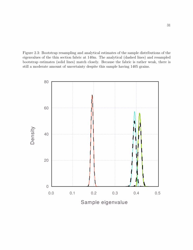
31
Figure 2.3: Bootstrap resampling and analytical estimates of the sample distributions of theeigenvalues of the thin section fabric at 140m. The analytical (dashed lines) and resampledbootstrap estimates (solid lines) match closely. Because the fabric is rather weak, there isstill a moderate amount of uncertainty despite this sample having 1405 grains.
Sample eigenvalue
0.0 0.1 0.2 0.3 0.4 0.50
20
40
60
80
Den
sity

32
Figure 2.4: Bootstrap resampling and analytical estimates of the sample distributions of theerror in fabric Euler angles of the thin section fabric at 140m. The analytical and resampledbootstrap estimates match closely. The smallest eigenvalue has a wide distribution in theassociated Euler angle, because the other two eigenvalues are close.
0
5
10
15
Den
sity
Fabric Euler angle error (rad)-3 -2 -1 0 1 2 3

33
Figure 2.5: Bootstrap 95% confidence intervals for enhancement factor for the 83 WAIS thinsections. Due to the dependence on the fourth power of the average Schmid factor, theconfidence intervals are wide.
0 500 1000 1500 2000 2500 3000 3500Ice depth (m)
0.0
0.5
1.0
1.5
2.0
2.5
3.0
3.5
4.0
4.5
Enha
ncem
ent f
acto
r

34
2.4 Conclusions
We compared PODFs with their log-likelihoods for different observed thin sections. This is
a standard technique to fit probability distributions. The Bingham distribution (Equation
2.3) and the Dinh-Armstrong distribution (Equation 2.4) perform nearly equally for the
WAIS and Siple Dome ice-core thin sections. Lliboutry’s Fisherian distribution (Equation
2.1) did not fit the thin sections as well. This is chiefly because the Fisherian distribution
assumes axial symmetry. Axial symmetry, which is an assumption used by many previously
proposed PODFs, is not capable of accurately approximating ODFs with three distinct fabric
eigenvalues. Ice fabric in most realistic situations has three distinct eigenvalues. However,
the ideal parameterized ODF may not be the same in all situations.
Inferring larger-scale bulk fabric from limited thin section samples is subject to sam-
pling error. We showed analytical estimates of eigenvalue and eigenvector sampling error.
Eigenvalue and eigenvector sampling error depends strongly on fabric strength, with single-
maximum fabrics having smaller eigenvalue and eigenvector variances than diffuse fabrics,
for the same sample size. Thus, to achieve the same certainty in fabric ODF, larger sample
sizes are needed for diffuse fabrics. We also examined bootstrapping of per-pixel EBSD or
automatic fabric analyzer measurements of thin section data. It is necessary to use block
bootstrapping for per-pixel data, rather than ordinary bootstrapping. Ordinary bootstrap-
ping neglects covariances between nearby pixels, which causes sampling error to be severely
underestimated. Sampling error estimates are sensitive to the grain size distribution. Often,
thin sections are dominated by a few large grains, with many smaller ones. This results
in much larger sampling uncertainties than even grain-size distributions. The estimates of
sampling error distributions for the WAIS core show that fabric eigenvalues are very poorly
constrained for some thin sections. Sonic fabric measurements are a promising way of over-
coming this inaccuracy (e.g., Diez and Eisen [19], Maurel et al. [57]).
These results indicate that fabric variability is likely important for small-scale flow. As
ice experiences power-law creep, relatively small variations in fabric strength can have a large

35
impact on flow. Volumes of several hundred to several thousand grains can be expected to
display a fairly large amount of fabric variability, indicating that ice flow characteristics are
unpredictable at those length scales. We may also expect regions of ice with larger grain-sizes
to experience significant fabric variability from sampling effects over larger length scales than
regions with small grain sizes, as a doubling of average grain radius will roughly double the
length over which sampling variability is important. Sampling variability may provide an
impetus for layer overturning or boudinage on small length scales.
Acknowledgements
We thank Joan Fitzpatrick and Don Voigt for the WAIS thin-section data. We also thank
Maurine Montagnat and Ilka Weikusat for helpful discussions on thin-section uncertainty.
This work was supported by the National Science Foundation grant 1246045.

36
Chapter 3
ICE FABRIC INFERENCE WITH THIN-SECTIONMEASUREMENTS AND SONIC VELOCITIES WITH
APPLICATION TO THE NEEM ICE CORE
This manuscript will be submitted to The Cryosphere Discussions soon, with co-authors
Erin Pettit, Ed Waddington, Dan Kluskiewicz, and Maurine Montagnat. Dan Kluskiewicz,
Erin Pettit, and others collected the sonic-velocity data. Maurine Montagnat gave us the
fabric eigenvalues. I developed the model and wrote this manuscript.
Abstract: We explore methods of inferring crystal orientation fabric using sound waves
in ice-core boreholes, in tandem with velocity data from ice-core thin sections. We pay
particular attention to sonic-velocity data collected from the NEEM ice core. Thin-section
fabric measurements have been the predominant way of inferring crystal fabric from bore-
holes. However, thin-section measurements suffer from sampling error, and do not provide
a spatially continuous record of fabric. Sonic-velocity measurements in boreholes allow for
spatially-continuous measurements of fabric, and largely eliminate sampling error. Unfortu-
nately, fabric inference from sonic-velocity measurements suffer from error associated with
the use of an imperfect sonic-velocity model (model error). In addition, the sonic tool used
at NEEM suffered from error due to poor tool centering in the borehole. It also collected
only P-wave velocities, which are sensitive only to the largest fabric eigenvalue. To address
these difficulties, we introduce a method to combine sonic-velocity measurements with fabric
measurements. We show that this new method suffers from significantly less sampling error
than thin-section measurements alone, while greatly reducing model error and the effects of
poor tool centering. In addition, this method provides a spatially-continuous record of all
three fabric eigenvalues, even if only P-wave data are available. We apply this method to

37
fabric thin-section data and sonic-velocity data collected at NEEM, to produce a spatially
continuous and accurate record of fabric.
3.1 Introduction
Ice is a highly viscoplastically anisotropic material, deforming most easily in shear parallel
to the basal plane, orthogonal to the crystallographic c-axis. The distribution of c-axis
orientations in a polycrystal is known as the orientation distribution function (ODF). The
bulk strain rate of a polycrystal can vary by an order of magnitude, depending on the ODF
[76]. The ODF is an antipodally-symmetric probability distribution on the sphere, giving the
density of c-axes by orientation across the sphere. Commonly, ODFs are summarized by the
second-order orientation tensor, which is the second moment A of the ODF. That is, it is the
average of the outer product of the c-axis with itself, c⊗c, taken over the ODF. Equivalently,
the second-order orientation tensor is the covariance matrix of c-axis directions. An estimate
A of the second-order orientation tensor can be found from a thin-section sample as,
A =∑i
ζici ⊗ ci, (3.1)
where there are N grains ci in the sample, with i = 1, .., N . Also, ζi is the area of grain i,
where the areas are normalized such that the total area of the thin section is unity.
The eigenvalues λi of this tensor provide a measure of fabric concentration in each of
the three corresponding eigenvectors, or fabric principal-directions. The largest eigenvalue,
λ3, is associated with the direction of the greatest c-axis concentration. The smallest, λ1, is
associated with the direction of least concentration. The middle eigenvalue, λ2, is associated
with the direction orthogonal to the other two. The eigenvalues sum to unity by construction.
If λ3 ≈ λ2 ≈ λ1, the fabric is isotropic. If λ3 � λ2 ≈ λ1, the ODF exhibits a single-maximum
fabric, with a large concentration in one direction. If λ3 ≈ λ2 � λ1, then the concentration
lies along a great circle orthogonal to the direction associated with λ1. This is known as a
girdle fabric.

38
If c-axis directions of a polycrystal are distributed uniformly across the sphere, the poly-
crystal has bulk isotropic viscosity. However, ice undergoing deformation develops a non-
uniform ODF. C-axes tend to rotate towards the directions of principal compression due to
lattice rotation during deformation [5]. This induces bulk anisotropic flow.
In ice sheets, ice crystals are usually somewhat randomly oriented at deposition, although
preferred orientations have been observed in the firn column close to the surface (Placidi et al.
[67], Durand et al. [27]). Vertical compression causes c-axes to rotate towards the vertical
direction. Likewise, shear on horizontal planes develops vertical-maximum fabrics due to the
combined pure shear and rotation. Near divides, horizontal extension in one direction, and
compression along the other two axes often causes vertical girdle fabrics to develop [5].
In addition to strongly affecting ice flow, the ODF seems to be sensitive to climate at
the time of deposition. Initial perturbations in fabric due to climate can persist into deep
layers [49]. In thin sections from the NEEM core [61], there is an abrupt change in fabric
corresponding to the Holocene boundary.
Orientation distribution functions are commonly estimated from ice thin sections taken
from ice cores, typically consisting of several hundred grains. This provides a direct sample
of the ODF from the section of ice, but suffers from sampling error. This sampling error
can be especially severe due to the typically highly non-uniform distribution of grain sizes.
Polycrystal properties are best weighted by area in the thin section [34]; if several large grains
cover much of the thin-section area, the effective sample size can be much smaller than the
number of sampled grains.
In addition to sampling error, thin-section samples have very limited spatial coverage,
usually on the order of 100 cm2. Thin-section samples are labor intensive and consume core
ice. Due to this, thin-section samples are typically taken only on the order of every tens of
meters. Therefore, thin-section samples cannot capture fabric variability at shorter length
scales. In addition, if one is interested in fabric characteristics averaged over several cubic
meters, rather than a single thin section, short length-scale fabric variability (on the scale of
decimeters) introduces another source of error.

39
Bentley [12] first proposed sonic logging as a method of fabric measurement to ameliorate
some of the difficulties of thin-section fabric measurements. In addition to being viscously
anisotropic, ice is elastically anisotropic. Therefore, sonic velocities of individual ice crystals
are dependent on grain orientation. The stiffness tensor of a polycrystal is dependent on the
orientation of the constituent grains. Sonic velocity measurements holds several advantages
over thin-section fabric measurements. Sonic logging tools can sample on the order of 3m3 of
ice [50], which nearly eliminates sampling error, and can reduce the influence of small-scale
variability in fabric.
Unfortunately, inference of fabric from sonic velocities is not straightforward. Model error
can be an issue. First, sonic velocity in ice is affected by pressure and temperature. P-wave
velocity in ice changes by around 2.5m s−1K−1 to 2.8m s−1K−1, which is a significant issue
in polythermal ice (e.g. Helgerud et al. [44], Vogt et al. [79]). This can cause differences in
velocity on the order of 100m s−1 in ice sheets [42]. Effects of temperature and pressure can
be corrected, but significant uncertainties may still remain.
Recently, Maurel et al. [57] developed analytical expressions for the elasticity tensors and
sonic velocities of ice for several ODF types. These included single-maximum fabrics with
c-axis density distributed uniformly within a given zenith angle from vertical. In addition,
they found solutions for idealized thick girdle and partial girdle fabrics. These relations have
since been applied by Smith et al. [71] to infer crystal fabric in the Rutford ice stream using
shear-wave splitting of seismic signals.
In this paper we outline a statistical model to infer fabric from sonic velocities using the
Google Tensorflow automatic differentiation library [1]. In contrast to Maurel et al. [57], we
model sonic velocities numerically using a flexible discrete ODF. This trades analyticity for
greater accuracy in ODF approximation.
We apply this technique to combine pseudo P-wave and thin-section measurements taken
from the NEEM ice core to find spatially continuous and more accurate fabric estimates. Un-
fortunately, the data collected from the NEEM core suffers from large velocity drift due to
poor tool centering in the borehole. In addition, model error may be significant. To correct

40
these errors, we incorporate thin-section measurements. While thin-section measurements
lack spatial coverage, and have significant sampling error, they are unbiased (although cor-
related) samples of the actual crystal fabric. If the systematic velocity error (due to bias or
model error) varies on length scales significantly larger than the spacing of the thin-section
measurements, then the thin-section measurements can be used to estimate this error. In this
way, we can combine the relative strengths of thin-section measurements (unbiasedness) and
sonic-velocity measurements (spatial coverage, little sampling error), while reducing their
weaknesses. We also test this technique on synthetic fabric data and sonic measurements,
and show that it can effectively correct velocity drift and model error.
3.2 Velocity model for sound waves in ice
We now outline the forward velocity model used to estimate sonic velocity from ice fabric.
Ice crystals exhibit anisotropic stiffness, dependent on c-axis direction. Bulk stiffness of ice
anisotropic polycrystals is therefore anisotropic, dependent on the orientation of individual
grains.
The bulk stiffness can be estimated using a volume-weighted average of the stiffness tensor
across the polycrystal,
Cijkl =
∫S2
ψ(c)Cijkl(c), (3.2)
where ψ is the ODF giving the density of c-axes at orientation c, and Cijkl(c) is the stiffness
tensor of an individual ice grain, with c-axis aligned to c in the bulk coordinate system. Esti-
mating bulk stiffness through volume-weighted stiffness assumes uniform strain throughout
the polycrystal. The other end-member instead takes the harmonic mean of the stiffness
tensor, which corresponds to a homogeneous-stress assumption. The truth is somewhere in
between these two [45], although both produce similar predictions. Here, we assume uniform
strain throughout the polycrystal, because it avoids numerical difficulties that occur with
small elements of the stiffness tensor under the harmonic mean.
Sonic velocities can be derived from plane-wave solutions to the elastodynamic wave

41
equation with zero forcing, (δij
d2
dt2− ρ−1Ciklj
d2
dxkdxl
)uj = 0, (3.3)
where ui is the material velocity of the polycrystal induced by the waves. Plane waves
are waves of the form ui = f(kixi − ωt)ui, where ki is the propagation direction, ui is the
polarization direction, and ω is the phase velocity. The function f is a scalar function of one
scalar argument. It may be a sine or cosine function, for example. Plugging the expression
for a plane wave into the above equation, the function f cancels out, and it can be seen that
admissible plane wave solutions are those where ui and ω2 are eigenvalue/eigenvector pairs
of the Christoffel matrix [4], whose components are given by,
Mij = ρ−1Ckijlkkkl. (3.4)
The Christoffel matrix is symmetric, because the stiffness tensor posesses symmetries such
that Ckijl = Cjlki = Cljik. The square roots of the three eigenvalues give the pseudo P-wave
velocity vp (the fastest), and the two pseudo-shear wave velocities, vsh (the slowest) and vsv
(intermediate speed). Unlike waves in isotropic media, the pseudo P-wave polarization is not
necessarily aligned with the propagation direction, and the shear waves are not necessarily
polarized orthogonal to the propagation direction. However, the polarizations are orthogonal
to one another because the Christoffel matrix is symmetric. Most observed fabrics in ice
sheets have a principal direction associated with the highest c-axis concentration which is
approximately vertical. Therefore, the pseudo P-wave velocity is typically polarized nearly
vertical.
As an alternative to stiffness averaging and solving the resulting Christoffel equations,
many authors have averaged the harmonic mean of sonic velocities (or the mean of the
slowness) across the ODF, instead of the stiffness tensor. While simple and intuitive, this
approach ignores mode conversion between P and S waves at grain boundaries [56].
We implemented this velocity model numerically by assuming that ice fabrics follow a
discrete ODF, where the support (the domain where probability density is nonzero) of the

42
distribution is confined to 900 “minimum energy” points cmepi [70], which are approximately
uniformly distributed over the sphere. Since the ODF is antipodally symmetric, we consider
only the points on the upper hemisphere. The distribution is parameterized by unconstrained
weights for each point, wi. In order for the distribution to add up to unity, the probability
measure at each point is given by,
ψ(cmepi ) =exp(wi)∑j exp(wj)
(3.5)
This is known as softmax normalization (e.g. Bouchard [14]). This distribution, which in
this paper we will refer to as the discrete approximating distribution, has many more param-
eters than a typical PODF. However, over-fitting can be avoided by introducing a quadratic
regularization penalty, similar to Tikhonov regularization. This is a very convenient distri-
bution to fit fabric eigenvalues and sonic velocities. The vast majority of PODFs do not have
analytical solutions for sonic velocities or eigenvalues in terms of their parameters. Thus,
these quantities usually need to be calculated by quadrature on the sphere. With this distri-
bution, we are “cutting out the middleman” by assuming beforehand that the distribution
is supported only on the quadrature points.
To find the bulk stiffness, we rotate the stiffness tensor (Equation 3.2) such that the
vertical axis of the transformed coordinate system is aligned with the c-axis of the quadrature
point point cmepi . This rotation is non-unique, since we assume that stiffness is invariant under
rotations about the c-axis (in other words, we are not attempting to measure a-axes). We
choose to rotate about the unique axis orthogonal to both cmepi and the vertical direction in
the global reference frame. Then, the bulk stiffness tensor is constructed by taking the sum of
the stiffness tensors for each point cmepi , weighted by the discrete approximating distribution
(Equation 3.5).
3.3 Fabric inference model
Fabric thin-sections provide a limited sample from the fabric ODF from where the sample
was taken. As discussed above, inference of the larger-scale ODF can have substantial error

43
from both sampling error and spatial nonstationarity of the ODF. Sonic measurements, on
the other hand, sample a large volume of ice, leading to extremely small sampling error.
In addition, the effects of sub-meter-scale spatial variability are significantly reduced. In
the NEEM core, only P-wave velocities were collected, which are not sensitive to azimuthal
fabric concentrations. In addition, the sonic data for the NEEM ice core have substantial
error varying slowly over longer length-scales, which we will refer to as drift. This contrasts
to the thin-section error, which is predominantly white noise stemming from sampling error
or short length-scale variability in the ODF. The thin-section measurements have less total
error when smoothing measurements over sufficiently long length-scales, but substantial error
over short length scales.
In this section, we develop a model to combine thin-section and sonic-log estimates of
fabric eigenvalues, while correcting for velocity drift and model error that varies smoothly
with depth. We do this by fitting the discrete approximating distribution (Equation 3.5) at
each depth, such that the modeled velocities derived from the discrete approximating fabric
distribution fit the thin-section data and the observed velocities as closely as possible.
This procedure requires several steps, which can be summarized as follows: First, we
use kriging [17] to fit the observed thin-section data. Next, at each depth, we fit the dis-
crete approximating distribution (Equation 3.5) to the thin-section eigenvalues. Then, sonic
velocities can be generated using the discrete approximating distribution, fitted to the thin-
section eigenvalues. This yields modeled sonic velocities from the thin-section data alone. If
significant velocity drift or smooth model error are present, there will be large, low-frequency
mismatches between the modeled velocity and observed velocities. This mismatch is distinct
from the higher-frequency mismatch due to thin-section sampling error or small-scale fab-
ric variability. The smooth velocity mismatch is then regressed out using kriging to yield
corrected velocities. Finally, the discrete approximating distribution is fitted to the cor-
rected velocities and the thin-section eigenvalues simultaneously. This then yields eigenvalue
estimates incorporating information from both sonic velocity and thin-section data.
To start with, we will use Gaussian-process regression [68], or kriging, to fit the observed

44
thin-section data. A Gaussian process is a random function f whose values yi = f(xi) at any
finite number of points xi follow a multivariate normal distribution. The covariance matrix
between sets of points X and X? is K(X,X?), where K is a positive-definite covariance
function, or kernel, giving the covariance between two points as a function of their location.
This induces a spatial structure in the Gaussian process. For example, a squared-exponential
(or, Gaussian) kernel is often used. Here, K is set to, K(X,X?) = k exp(−b||X − X?||2),where b is a constant giving the bandwidth of the Gaussian, and k is a scaling parameter.
This favors smooth functions, because the correlation of nearby points is unity to first order.
Gaussian white noise is also a Gaussian process, whose covariance function is K(x,x?) = a if
x = x?, and zero otherwise. This indicates that the values at different points are uncorrelated
but the value at a given point follows a univariate normal distribution.
Rather than working with eigenvalues directly, we instead fit the ηi:
ηi = logit(λi) = log(λi)− log(λ3). (3.6)
While the fabric eigenvalues are constrained to sum to unity, the logit eigenvalues ηi can take
on any value. This makes the logits much easier to work with because the sum constraint is
removed. The corresponding inverse softmax transformation squashes the logits back such
that they sum to unity:
λi = softmax(ηi) =exp(ηi)∑j exp(ηj)
. (3.7)
We assume that each of the observed logit-transformed eigenvalues ηi are drawn from a
realization of a Gaussian process, whose prior covariance is given by the sum of an expo-
nential covariance function, exp(−a||xi − xj||), and a white noise covariance function. The
exponential kernel allows for discontinuous functions, because the nearby points are not per-
fectly correlated to first order (as is the case with the squared-exponential kernel). This is
a more realistic covariance function than the squared-exponential covariance function, since
observed fabric eigenvalues do seem to change abruptly with depth. From this, the predictive
mean of the logit eigenvalues at a depth d′, conditioned on the observed logit eigenvalues ηts

45
at depths dts, is given by,
ηi(d′) = K(d′,d′
ts)K−1(dts,dts)ηtsi , (3.8)
The predictive variance of the the estimated logit eigenvalue ηi at depth d′ is,
Var(d′) = K(d′)−K(d′,dts)K−1(dts,dts)K(dts, d′) (3.9)
This mean and variance defines a normal distribution for the logit eigenvalues ηi at each
depth. From this, at each depth d′ we can fit the discrete approximating distribution (Equa-
tion 3.5) to these eigenvalues. This is done by minimizing the squared error between the
predicted mean of ηi at depth d′, given by Equation (3.8), and the calculated fabric eigen-
values from the discrete approximating distribution (Equation 3.5). This is given by the
eigenvalues of the estimated second-order orientation tensor A of the discrete approximating
distribution (Equation 3.5):
A =∑c∈M
ccTψ(c), (3.10)
where M is the set of minimum-energy points. If we assume that the fabric has a principal
direction oriented nearly vertical, then the estimated eigenvalues λi are given by the diagonal
elements Aii (no sum) to first order.
From this, at each depth we have fitted the discrete approximating distribution to the
observed thin-section data, but not the observed velocities. We then calculate modeled sonic
velocities, given the thin-section data. The calculated sonic velocities do not suffer from the
drift of the observed sonic velocities, and are approximately correct on longer length scales,
unlike the observed sonic velocities. However, due to the usually low spatial coverage of
thin sections, the calculated sonic velocities do not detect the meter-scale features of fabric
that the sonic-velocity measurements can (since the velocity measurements are taken nearly
continuously with depth). We approximately correct this mismatch by using Gaussian-
process regression to estimate the mismatch under the assumption that it is smooth. This
will not remove the non-smooth, higher-frequency components of the velocity mismatch,
which can instead be expected to correspond to actual short length-scale fabric variability,

46
which is not captured by thin-section measurements. For each velocity vi (either vsh, vsv, or
vp) the mismatch at a depth d′ is,
εi(d′) = vtsi (d′)− vobsi (d′), (3.11)
where vobsi (d′) is the observed velocity at depth d′, and vtsi (d′) is the modeled velocity from the
thin-section data. Here, we take the covariance function to be a sum of a squared-exponential
covariance function, and white noise. This is given by,
Kεi(d, d′) = kεi exp(−aεi ||d− d′||2) + σ2
εiI(d− d′), (3.12)
where kεi and σ2εi
are scaling parameters, and aεi is the bandwidth. I is a function where
I(0) = 1, and I(z) = 0 for z 6= 0. This covariance produces smooth predictions, encoding
a belief that the velocity drift is smooth. Similar to the Gaussian-process regression of the
logit-transformed eigenvalues, the predicted mean of the the velocity mismatch is,
εi(d′) = Kεi(d
′,dts)K−1εi (dts,dts)εtsi . (3.13)
The modeled velocity is found from Equation (3.4). This then gives us the corrected veloci-
ties, with mean vcorri = vobsi + εveli . Finally, at each depth d′, we simultaneously fit the discrete
approximating distribution to the corrected velocities (Equation 3.13) and the inferred thin-
section logit-transformed eigenvalues ηi(d′) (Equation 3.8). This is done by minimizing the
following quantity with respect to the weights w of the discrete approximating distribution
at each depth of interest,
J(w) =σ−2sh (vsh(w)− vcorrsh )2 + σ−2sv (vsv(w)− vcorrsv )2+
σ−2p (vp(w)− vcorrp )2 + σ−2η1 (η1(w)− η1)2+
σ−2η2 (η2(w)− η2)2 + σ−2η3 (η3(w)− η3)2 + α||w||2. (3.14)
Here, σ2sh is the variance of the velocity estimation, given by the sum of the variance of the
velocity-correction term and the variance of the sonic-velocity measurements. The quantities
σsv and σp are defined similarly. The quantity σ2ηi
is the variance of the posterior Gaussian

47
process estimation of the logit-transformed fabric eigenvalue ηi, given by Equation 3.9. The
last term α||w||2 is a regularization term, equivalent to putting a zero-mean Gaussian prior
on the weights w. This regularization term serves only to ensure that a unique minimum
exists for the objective function (3.14), rather than representing any kind of prior knowledge.
The term is small enough that any fabric eigenvalues can be fit almost exactly. We minimized
J with respect to w using Adagrad gradient descent [23], with the gradients derived using
the Google Tensorflow automatic differentiation package [1].
Note that the objective function (3.14) is optimized independently at each depth of
interest. We do not assume any kind of prior knowledge of smoothness with depth for this
objective function. Sonic data collected from sonic tools are best averaged over a length-scale
similar to the distance between the two sonic receivers. This accounts for short length-scale
spatial correlations. There is no reason to assume a that fabric over longer length-scales
is significantly correlated, since fabrics do indeed vary significantly over short length-scales.
Assuming smoothness over longer length-scales would not allow for such short length-scale
variability.
3.4 Eigenvalue inference on synthetic data
We now evaluate the statistical model developed in the previous section on synthetic fabric
data. We generated “true” fabric eigenvalues for a 3000m deep borehole by assuming that
the logit-transformed eigenvalues are sampled from a Gaussian process with an exponential
covariance function, to yield eigenvalues that are discontinuous with depth. We then generate
“true” vp, vsh, and vsv velocities from these eigenvalues. We then add a smooth velocity
corruption to these velocities (corresponding to model error and velocity drift), to yield
synthetic corrupted velocities. The velocity corruption is the same absolute value for vsh,
vsv and vp. However, we do not use this knowledge in fitting the model. Instead we fit a
separate correction for each velocity. Synthetic thin-section samples were generated every
30m by adding noise averaging 0.2 to the logit-transformed eigenvalues at each depth, with
100 thin sections in total.

48
0 500 1000 1500 2000 2500 3000Depth (m)
0.0
0.2
0.4
0.6
0.8
1.0
Eig
envalu
e
True λ1
True λ2
True λ3
Modeled λ1
Modeled λ2
Modeled λ3
Thin section λ1
Thin section λ2
Thin section λ3
Figure 3.1: Application of the statistical model to synthetically generated fabric. Thin-section eigenvalues with 30m spacing are generated by adding noise to the true eigenvalues.The modeled eigenvalues are close to the true eigenvalues over the majority of the depth.Error is primarily due to error in the velocity-correction term.

49
The results are plotted in Figure 3.1. Over the majority of the core, the true fabric
eigenvalues are approximated accurately. In a few spots, larger errors occur due to mis-
estimation of the velocity corruption. The estimated velocity corrections and the true velocity
corruption are plotted in Figure 3.2. Typical errors are on the order of 10ms−1.
Note that we do not add white noise to the synthetic velocity data, which would cor-
respond to sonic velocity measurement error uncorrelated with depth. We expect that un-
certainties in arrival times are the primary cause of non depth-correlated velocity errors.
With velocities averaged over several runs, and smoothed over a few meters, this error would
typically be small in comparison to the depth-correlated errors of model error and velocity
drift.
This is a challenging synthetic dataset, with large high-frequency spatial variability in
eigenvalues. With only 100 noisy thin-section measurements, it can be difficult to separate
the effects of the velocity corruption from actual variability in fabric eigenvalues. More thin
sections, or less fabric variability can reduce this substantially.
3.5 Application to sonic measurements at NEEM
In this section, we apply the statistical model to P-wave velocity data and thin-section data
collected at NEEM [61]. Unlike the case with synthetic data, only P-wave velocities were
collected. The P-wave velocity constrains only the concentration of c-axes in the vertical
direction (associated with the largest fabric eigenvalue λ3). However, due to the sum con-
straint of eigenvalues, this still provides information on the sum of λ1 and λ2. The data were
collected with a Mount Sopris CLP-4877 sonic-logging tool, modified to have a larger receiver
spacing. The tool emits a monopole impulse source, which travels through the borehole fluid,
through the ice, and back through the borehole fluid to two recievers, spaced at 90cm and
303.5cm from the source. Pulses are emitted every 2µs.
Three separate sonic logs were completed, with several sonic measurements taken every
meter. Since the tool itself is roughly 3m long, spatial variability in sonic velocities shorter
than 3m are difficult to interpret. Thus, in our analysis, we take 3m moving averages of the

50
0 500 1000 1500 2000 2500 3000Depth (m)
140
120
100
80
60
40
20
Velo
city
(m
/s)
True velocity driftEst. vsh drift
Est. vsh drift
Est. vp drift
Figure 3.2: Velocity corruption (dashed) and estimated velocity corrections (solid lines)for vp, vsh, and vsv. Estimation of the velocity corruption depends on the thin-sectioneigenvalues. Due to the large degree of spatial variability of the fabric, and the noise in thethin sections, inaccuracies on the order of 10m/s occur. More thin-section samples, and moreaccurate samples, can reduce this error substantially.

51
data. This also serves to significantly reduce uncorrelated measurement error, reducing error
in measured vp due to uncertainties in arrival times to the order of 1mi s−1 over multiple
runs [50].
As discussed previously, large velocity drift occurs due to poor tool centralization in the
borehole. This can differ between runs of the logging tool. However, short length-scale
features are consistent between between runs.
We use the thin-section data from Montagnat et al. [61]. There are 271 thin sections,
taken from 34m to 2461m. At some depths, multiple thin sections are taken. This gives
a rough indicaton of the sampling error of the thin sections at those depths. We apply
the model only below 250m. Above this depth, the velocity model becomes increasingly
inaccurate. We expect this is due to a higher concentrations of air bubbles in the ice.
In Figure 3.3, we plot the modeled P-wave velocities from NEEM thin sections, and the
collected P-wave velocities. There is a significant mismatch, with the collected P-wave data
typically being on the order of 100m s−1 less than the modeled P-wave velocities. The lower-
frequency part of this mismatch is due to some combination of model error and velocity
drift. We expect both to be smooth, as the assumptions of the statistical model require.
In addition to these smooth errors, the velocities derived from thin sections have significant
uncertainties due to sampling error.
In Figure 3.4, we plot the eigenvalues derived from thin sections along with eigenval-
ues estimated using both thin-section data and the collected P-wave velocity. The largest
eignvalue λ3 increases almost linearly in the first 1300m of the core. Below about 2000m,
the modeled eigenvalues begin to display large, high-frequency spikes. This may be due to
differing amounts of recrystallization between layers. Layers experiencing greater amounts
of recrystallization tend to have weaker fabrics. These fabric contrasts may also help initiate
flow disturbances near the bed.
Applied to the NEEM ice-core data, we believe this model produces very accurate predic-
tions of the largest eigenvalue, λ3. Other eigenvalues are not informed by the P-wave velocity,
except due to the eigenvalue sum constraint. While the P-wave data provide information on

52
0 500 1000 1500 2000 2500Depth (m)
3800
3850
3900
3950
4000
4050
4100
P-w
ave v
elo
city
(m
/s)
Measured P-wave velocitiesModeled P-wave vel. at thin sections
Figure 3.3: P-wave velocities modeled from thin sections (dots) and observed P-wave ve-locities (line). The observed P-wave velocities are smoothed over 3m and are averaged overmultiple runs. Due to a combination of model error and velocity drift, the observed velocitiesare on the order of 100m s−1 less than the modeled velocities.
the sum of λ1 and λ2, it does not inform the difference between the two.
There are more thin sections, and much less large spatial variability in the NEEM core
compared to the test on synthetic fabric. Thus, we expect the estimation of the velocity-
correction term in the model to be more accurate, resulting in more accurate predictions
of the largest eigenvalue λ3 compared to the results for the synthetic data. Error in thin
sections in estimating the eigenvalues of the bulk fabric (in volumes sampled by the sonic
tool) is on the order of 0.1 over most of the core, increasing in the recrystallized deep layers.
These errors correspond to larger uncertainties in ice viscosity, due to the power-law rheology
of ice.
3.6 Conclusions
We showed P-wave velocity data collected from the NEEM ice core with a borehole sonic-
logging tool. The collected P-wave velocities provide a high-quality continuous record of

53
0 500 1000 1500 2000 25000.0
0.2
0.4
0.6
0.8
1.0
Modeled λ1
Modeled λ2
Modeled λ3
Thin section λ1
Thin section λ2
Thin section λ3
Figure 3.4: Eigenvalues derived from thin sections at NEEM (dots) [61], together withspatially-continuous estimates from the assimilation procedure. The variability of eigenvaluesover shorter length scales in the upper core appears to be due to sampling error. The largevariations seen in the thin sections in the deep ice are confirmed by the sonic velocity data.
fabric over depth at scales longer than 2m. However, they are subject to smoothly-varying
errors.
We derived a method of incorporating thin-section data and sonic-velocity data in order
to gain a more accurate, and spatially continuous picture of the ODF. This is especially
important for understanding stratigraphic disruption that occurs near the bed of NEEM
and other cores. The inferred fabric from the NEEM core shows variability in fabric on
the order of several meters. This may trigger or enhance stratigraphic disruption. Fabric
variability on these length scales is impossible to observe with thin sections taken only every
several meters, with large sampling error.
This work demonstrates the utility of combining different methods of ODF measure-
ments. Future work measuring S-wave velocities will greatly enhance the capabilities of
sonic-velocity measurements in ODF determination. Improved sonic tools could reduce ve-
locity measurement error and bias. However, we still expect that thin-section measurements
54
are a useful adjunct to provide a mostly unbiased ground-truth for ice-sheet fabric to correct
velocity-model error.

55
Chapter 4
THE RESPONSE OF ICE-CRYSTAL ORIENTATION FABRICTO VELOCITY-GRADIENT PERTURBATIONS
This chapter is under review at the Journal of Glaciology. Ed Waddington is a co-author.
I developed the analytical and numerical models, and wrote this manuscript.
Abstract: The distribution of crystal orientations of ice grains (the crystal fabric) of
a polycrystal has a strong influence on the flow of polycrystalline ice, due to the plastic
anisotropy of the individual grains. The fabric is in turn affected by ice flow. Flow on
ice-sheet flanks is dominated by shear on horizontal planes, and divide flow is dominated
by longitudinal extension. However, other velocity gradient components may also exist
due to bed topography, variability in fabric or grain size, or other factors. This can in
turn result in a fabric that differs from the fabric that would occur without any such flow
disturbances. Indeed, disturbed stratigraphy is commonly observed near the bed of ice
sheets. In this paper, we treat these flow disturbances as random but correlated in time,
and determine their effects on crystal fabric. These small deviations in velocity gradient
from pure shear or simple shear can induce the development of single-maximum fabrics with
off-vertical directions of maximum c-axis concentration. In turn, this has the potential to
induce stratigraphic distortion.
4.1 Introduction
An individual ice crystal deforms most easily in shear parallel to the crystal basal plane,
orthogonal to the crystallographic c-axis. Deformation on planes in other orientations is on
the order of 10 to 100 times harder. Plastic deformation of an ice polycrystal depends on
the orientations of its constituent grains (e.g. Azuma [8]), which is described by the c-axis
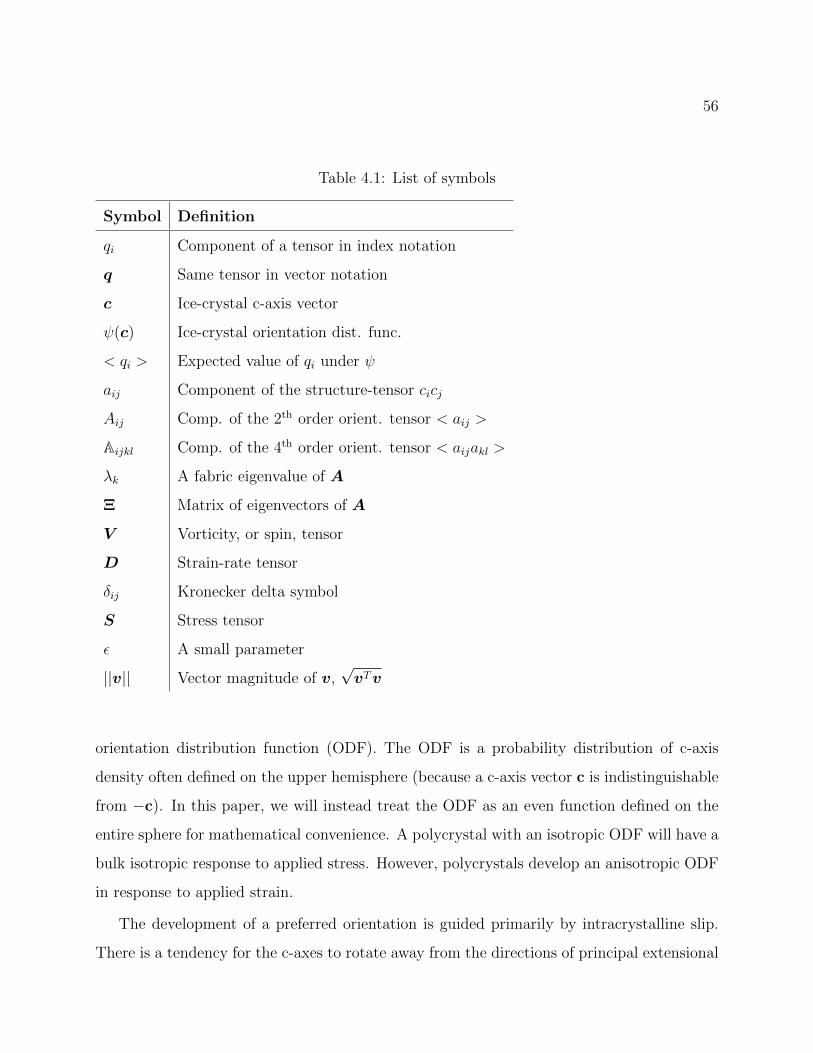
56
Table 4.1: List of symbols
Symbol Definition
qi Component of a tensor in index notation
q Same tensor in vector notation
c Ice-crystal c-axis vector
ψ(c) Ice-crystal orientation dist. func.
< qi > Expected value of qi under ψ
aij Component of the structure-tensor cicj
Aij Comp. of the 2th order orient. tensor < aij >
Aijkl Comp. of the 4th order orient. tensor < aijakl >
λk A fabric eigenvalue of A
Ξ Matrix of eigenvectors of A
V Vorticity, or spin, tensor
D Strain-rate tensor
δij Kronecker delta symbol
S Stress tensor
ε A small parameter
||v|| Vector magnitude of v,√vTv
orientation distribution function (ODF). The ODF is a probability distribution of c-axis
density often defined on the upper hemisphere (because a c-axis vector c is indistinguishable
from −c). In this paper, we will instead treat the ODF as an even function defined on the
entire sphere for mathematical convenience. A polycrystal with an isotropic ODF will have a
bulk isotropic response to applied stress. However, polycrystals develop an anisotropic ODF
in response to applied strain.
The development of a preferred orientation is guided primarily by intracrystalline slip.
There is a tendency for the c-axes to rotate away from the directions of principal extensional

57
strain due to lattice rotation [10]. ODFs are often summarized using orientation (or, moment)
tensors (e.g. Svendsem and Hutter [73]), where the nth order moment tensor is the nth order
moment of the ODF. Throughout this paper, the indices 1, 2, and 3 will be associated
with the x-, y-, and z-directions, respectively. Fabric is usually described using only the
second-order orientation tensor A. The component of the second-order orientation tensor
Aij is the expectation < cicj >, where i, j = 1, 2, 3. The mean of the ODF (or the first-order
orientation tensor in this terminology), < ci >, is always zero because of antipodal symmetry
(and likewise for any odd-order tensor). Therefore, Aij is also a component of the covariance
tensor of the distribution:
Cov(ci, cj) =< (ci− < ci >)(cj− < cj >) >
=< (ci − 0)(cj − 0) >
= Aij (4.1)
The diagonal elements A11, A22, and A33 give a measure of the c-axis concentration on the x,
y, and z axes, respectively. Similar to the second-order orientation tensor, the fourth-order
tensor is the expected value Aijkl =< cicjckcl >. Since the second-order orientation tensor
is symmetric, it is diagonal in the coordinate system defined by its eigenvectors, or fabric
principal directions. The diagonal elements are the fabric eigenvalues λi. The eigenvalues
sum to unity by construction. The three fabric principal directions denote the directions
of greatest density (corresponding to the largest eigenvalue), smallest density (the smallest
eigenvalue), and a direction orthogonal to the other two. An isotropic fabric has three equal
eigenvalues. A girdle fabric (in which there is a band of high concentration along a great
circle) has two nearly equal eigenvalues, and one small eigenvalue. A single-maximum fabric
has one large eigenvalue, and two small eigenvalues.
If the evolution of the ODF is given by a partial differential equation (PDE) over the
sphere, it is possible to derive an ordinary differential equation (ODE) for the evolution
of Aij. This is much easier than solving the PDE, whose solution at any given time is

58
a function defined on the sphere, rather than just the six unique elements of the second-
order orientation tensor. This substantially reduces computational difficulties. With this
approach, Gillet-Chaulet et al. [38] used a Jefferys-type equation for Aij, valid when the c-
axes move by basal slip only. Their model works for arbitrary vorticity tensors and velocity
gradients. Godert [40] developed a similar model incorporating rotary diffusion into the
evolution equation for Aij. In this paper, we take a similar approach to Gillet-Chaulet et al.
[38].
Fabric development during ice flow is likely a physically deterministic process. However,
at any given site, there are uncertainties in strain history, impurity content, initial conditions
at deposition, and other factors. We examine how these uncertainties may affect uncertain-
ties in ice flow. Flow inhomogenities can result from numerous sources. On small scales,
random variations in fabric strength can in turn induce spatial differences in flow. Near the
bottom of the West Antarctic Ice Sheet (WAIS) divide core, some layers have experienced
recrystallization, and have a weaker fabric compared to others that have not recrystallized
[30]. Durand et al. [25] found an abrupt transition in the ice fabric at EPICA Dome C
corresponding to Termination II, suggesting that climate at the time of initial deposition
can play a prominent role in in the subsequent development ice fabric. Alley et al. [7] found
evidence of “striping” in the GISP2 core, in which elongated areas of grains possessed off-
vertical c-axes. In horizontal extension under divide flow, these stripes localize shear within
them, and offset layers in the hard surrounding ice. This induces flow disturbances around
stripes, as well as overturning stratigraphic layers. Jansen et al. [47] produced bands similar
to observed stripes in strong single-maximum fabrics using the two-dimensional ELLE mi-
crostructure model. Regions where the fabric was tilted away from the bulk lattice-preferred
orientation toward the direction of shear seeded the formation of the bands. On larger scales,
flow disturbances can arise due to basal topography and transient flow, basal-ice accretion
[11], or various other sources.
Thorsteinsson and Waddington [76] examined the development of low-angle wrinkles
in stratigraphic layers in ice sheets. Under simple shear, low-angle wrinkles will steepen,

59
Figure 4.1: The six unique components of A for 3000 realizations of the Jeffery’s-typeequation (5.7) forced with pure shear and a strain perturbation whose components average2% of the background pure shear, and γ = 1. The central 95% of realizations are shaded.Significant deviations of A13 and A23 occur. These correspond to tilted cone fabrics whosedirection of greatest concentration differs on the order of 5◦ from vertical.
1 2 3 4 5 6 7 8 9 10
Total strain
0.0
0.2
0.4
0.6
0.8
1.0A11
1 2 3 4 5 6 7 8 9 10
Total strain
0.0
0.2
0.4
0.6
0.8
1.0A22
1 2 3 4 5 6 7 8 9 10
Total strain
0.0
0.2
0.4
0.6
0.8
1.0A33
1 2 3 4 5 6 7 8 9 10
Total strain
−0.4
−0.2
0.0
0.2
0.4
A23
1 2 3 4 5 6 7 8 9 10
Total strain
−0.4
−0.2
0.0
0.2
0.4
A13
1 2 3 4 5 6 7 8 9 10
Total strain
−0.4
−0.2
0.0
0.2
0.4
A12

60
eventually producing overturned folds. Pure shear or vertical uniaxial compression produce
the opposite effect, flattening out wrinkles. Near ice divides, simple shear is less prominent
compared to pure shear. However, vertical single-maximum fabrics develop under both
vertical compression and simple shear. These fabrics make the ice harder under vertical
compression, and soft under horizontal simple shear. This may greatly aid the development
of stratigraphic disruption in simple shear, because steepening of incipient folds is enhanced,
while flattening is reduced.
In this paper, we analyze how small amounts of variability in the velocity gradient can
affect crystal fabric. By “variability,” we mean small components of the velocity gradient
distinct from the dominant background flow (e.g., simple shear in flank flow). The goal is
to see whether it is possible to develop large excursions in the ODF in response to small
velocity-gradient perturbations. If, as a result of small excursions in the velocity gradient,
large, spatially non-homogeneous differences in fabric can develop, they may seed further
velocity gradient disturbances and stratigraphic disruption. We do not examine sources of
such flow disturbances. Instead, we make the approximation that they are random, but
correlated in time. That is, the perturbation at a certain time will be highly correlated to
perturbations at sufficiently nearby times.
This paper is split into two main parts. In the first section, we develop a first-order
approximation of the effects of a velocity-gradient perturbation on concentrated vertical
single-maximum fabrics in flank flow (horizontal simple shear) and divide flow (pure shear).
We show that in both cases, small perturbations of the velocity gradient can cause the fabric
principal directions to rotate significantly, generating a fabric that would induce a vertical
velocity perturbation in both flow situations. In the second section, we expand on the
analytical result by numerically solving the Jeffery’s-type equation for the evolution of Aij
(see next section) perturbed by a small random velocity gradient. We generate confidence
intervals of the six unique components of Aij by computing several thousand realizations.
The results numerically confirm the analytical observations in the first section.

61
4.1.1 Fabric evolution
The most important process governing the development of crystal fabrics is deformation-
induced grain rotation. If grain deformation is due solely to basal glide, the rate of change
of the c-axis orientation is the sum of bulk rotation and viscoplastic spin. From Meyssonnier
and Philip [58], the evolution of c-axis orientation in response to strain can be described by
a modified Jeffery’s equation [48]:
ci = Vijcj −Dgijcj + cicjckD
gjk, (4.2)
where ci is the unit vector in the direction of the c-axis. The quantities Vij and Dgij are
components of the rotation-rate tensor, and local strain-rate tensor of the grain, respectively.
The first term gives the rotation rate due to the bulk rotation of the polycrystal, while the
second term gives the rotation rate due to viscoplastic spin. Thus, for example, the c-axis of
a grain experiencing uniaxial compression will rotate towards the compressive direction. The
last term of Jeffery’s equation (5.2) ensures that the motion of grain orientation is tangent
to the unit sphere at c, which is necessary due to the convention that the c-axis vector is of
unit length. This can be seen by noting that the Vijcj term does not affect the magnitude of
ci, leaving only the Dijcj term. Assume that at time t = 0, the c-axis is given by c0. After
a short length of time δt, the magnitude of the new c-axis cδt is (without the final term in
Equation 5.2),
||cδt|| = ||c0 − δtDc|| (4.3)
≈ ||c0||−cT0Dc0δt (4.4)
= 1− cT0Dc0δt, (4.5)
to first order in δt. Thus, for the c-axis to maintain unit length, we must add the quantity
cTDcδt projected onto c, by multiplying by c. This then gives the last term of Equation
(5.2). Rather than compute the rotation rate for each grain individually, we instead seek an
evolution equation for the second-order orientation tensor whose components are given by
62
Aij =< cicj >. Differentiating with respect to time, we have,
dAijdt
=< cicj > + < cicj > . (4.6)
This introduces the problem of homogenization. We must average out the quantity in the
brackets over the entire ODF. However, cki , for some individual grain k, depends on the strain-
rate tensor of that particular grain as can be seen in Equation (5.2). Thus, we need a tractable
method for relating the bulk stress and strain to that of individual grains. The stress and
strain of each individual grain should ideally be consistent with the bulk stress and strain rate.
The two possible end-members are the Taylor-Bishop-Hill model [74], assuming homogeneous
strain among grains, and the Sachs model [69], which assumes homogeneous stress among
grains. Visco-plastic self-consistent (VPSC) homogenization methods [52] have been used
for anisotropic ice-flow constitutive relations (e.g. Castelnau et al. [15], Gillet-Chaulet et al.
[38]). VPSC schemes treat each individual grain as an ellipsoidal inclusion in a medium with
the average properties of the polycrystal. This can provide a more accurate distribution
of stress and strain within the polycrystal, with stress and strain both dependent on the
orientation of a grain. Grain rotation due to lattice rotation can also be directly incorporated
into VPSC schemes. However, VPSC schemes are typically computed iteratively over finite
samples of grains, and are difficult to directly incorporate into Eq. (4.6).
As a compromise, Gillet-Chaulet et al. [37] took the strain on an individual grain as a
weighted average between the homogeneous stress and homogeneous strain assumption. In
this case, Dgij in Eq. 5.2 is,
Dgij = (1− α)Dij + α
ςSij2, (4.7)
where Dij is a component of the bulk strain-rate tensor, Sij is a component of the bulk stress
tensor, and ς is the fluidity for shear parallel to the basal plane. The weighting between
homogeneous stress and homogeneous strain is given by the interaction parameter α. Setting
α = 0 gives the homogeneous strain rate assumption, while α = 1 gives homogeneous stress.
This parameter may be tuned to fit a VPSC model. In Gillet-Chaulet et al. [38] they used
a value of α = 0.06. Throughout this paper, we use the homogeneous strain assumption,

63
with α = 0. The homogeneous strain assumption for grain rotation produces fairly realistic
predictions for fiber orientation, even though the homogeneous strain assumption produces
rather poor predictions of ice flow. Given that Gillet-Chaulet et al. [38] found the best
results with α = 0.06, we are not too far off by setting α = 0. Note that setting α 6= 0
to yield a local grain strain rate equal to Gij produces the same predictions as assuming
homogeneous strain, and setting the bulk strain Dij = Gij. For vertical single-maximum
fabrics forced with simple shear or pure shear, as in this paper, Dij and Sij are proportional
with dimensions of viscosity.
With this assumption, the derivative of the second-order orientation tensor A becomes,
dAijdt
=VikAkj − AikVkj −DikAkj − AikDkj+
2AijklDkl.
(4.8)
The presence of the fourth-order orientation tensor Aijkl in Eq. (5.7) introduces the closure
problem. In general, Aijkl cannot be found from A. If we used an additional evolution
equation for Aijkl, then the six-order orientation tensor would appear in that equation, and
so on. Thus, we need some way of approximating Aijkl in terms of A. In this paper, we use
the popular and simple quadratic closure, where Aijkl = AijAkl [3]. This closure is exact in
the case of perfectly concentrated single-maximum fabrics, where Aij = δi3δj3. It is quite
accurate whenever λ3 > 0.8 or so. In this paper, we are primarily intersted in the response
of strong fabrics to velocity-gradient perturbations, so this is a good approximation for our
purposes.
4.2 First-order perturbations to strong single-maximum fabrics
We now examine the analytic sensitivity of strong vertical-maximum fabrics to velocity-
gradient perturbations. We show that fabrics are susceptible to developing “tilted cone”
fabrics, in which the direction of greatest concentration is not vertical, in both horizontal
pure shear and simple shear. Here we add a small perturbation εAij to the component of
the second-order orientation tensor Aij. The tensor A has zero trace, and ε is small. Then,

64
Figure 4.2: The six unique components of A for 3000 realizations of the Jeffery’s-typeequation (5.7) forced with pure shear and a strain perturbation whose components average 5%of the background pure shear, with γ = 1. the central 95% of realizations are shaded. Largerdeviations of A13 and A23 occur than under 2% average perturbations. These correspond totilted cone fabrics tilted on the order of 10◦ from vertical. The background pure shear isvery effective at restraining perturbations of other components of A.
1 2 3 4 5 6 7 8 9 10
Total strain
0.0
0.2
0.4
0.6
0.8
1.0A11
1 2 3 4 5 6 7 8 9 10
Total strain
0.0
0.2
0.4
0.6
0.8
1.0A22
1 2 3 4 5 6 7 8 9 10
Total strain
0.0
0.2
0.4
0.6
0.8
1.0A33
1 2 3 4 5 6 7 8 9 10
Total strain
−0.4
−0.2
0.0
0.2
0.4
A23
1 2 3 4 5 6 7 8 9 10
Total strain
−0.4
−0.2
0.0
0.2
0.4
A13
1 2 3 4 5 6 7 8 9 10
Total strain
−0.4
−0.2
0.0
0.2
0.4
A12
components of the perturbed second-order orientation tensor are given by Aij = Aij + εAij.
Next, we also assume that the vorticity and strain rate are perturbed by small quantities
εV and εD, respectively. Then, we can substitute these quantities into Eq. (5.7), and discard
quantities of O(ε2) and higher. This then gives us a first-order equation for the perturbed

65
As with the case of pure shear, the only components that are directly affected by velocity-
gradient perturbations (to first order) are A13 and A23. The growth of the perturbation A13
to A13 is affected by A22. Depending on the signs of D13 and V13, it may be restrained or
reinforced by A22. Similarly, other components depend on each other, to first order. For
example, A11 depends negatively on A13. However, we may expect that A13 and A23 will
generally be the largest components of A in magnitude. As long as their magnitudes are

66
Figure 4.3: The six unique components of A for 3000 realizations of the Jeffery’s-typeequation (5.7) forced with simple shear and a strain perturbation whose components average2% of the background pure shear, with γ = 1. The central 95% of realizations are shaded.Smaller perturbations develop than with pure shear. However, they still may be enough toseed further fabric and flow disturbances.
1 2 3 4 5 6 7 8 9 10
Total strain
0.0
0.2
0.4
0.6
0.8
1.0A11
1 2 3 4 5 6 7 8 9 10
Total strain
0.0
0.2
0.4
0.6
0.8
1.0A22
1 2 3 4 5 6 7 8 9 10
Total strain
0.0
0.2
0.4
0.6
0.8
1.0A33
1 2 3 4 5 6 7 8 9 10
Total strain
−0.4
−0.2
0.0
0.2
0.4
A23
1 2 3 4 5 6 7 8 9 10
Total strain
−0.4
−0.2
0.0
0.2
0.4
A13
1 2 3 4 5 6 7 8 9 10
Total strain
−0.4
−0.2
0.0
0.2
0.4
A12

67
generally less than the applied velocity-gradient perturbations, perturbations to other com-
ponents will grow more slowly. For example, if |−2A13|, the growth rate of the perturbation
to A11, is less than |A22 − D13 + W13|, the growth rate of A13, we can expect A13 to grow
faster than A11. This intuition is confirmed numerically in the next section.
4.3 Monte-Carlo analysis of stress perturbations
We now expand on the sensitivity analysis of the previous section by considering numerical
solutions to the Jeffery’s equation (5.7) forced with background simple shear or pure shear
in addition to a small random velocity gradient. This gives us an idea of the magnitude of
fabric perturbations that we may expect in response to velocity-gradient perturbations. It
also allows us to look at the effects of velocity-gradient perturbations away from equilibrium.
In the previous section, we showed that background pure shear or simple shear is not effective
at restraining perturbations of the A13 and A23 components of the second-order orientation
tensor. Integrating the Jefferys equation (5.7) through time, we can expect the effects of
velocity-gradient perturbations to be magnified, as integration acts as a low-pass filter.
First, we must have some way of generating velocity-gradient perturbations. It is reason-
able to assume that a velocity-gradient perturbation at time t will be highly correlated to
perturbations at t + ε, if ε is small enough. To account for this, we construct the velocity-
gradient perturbations using realizations of a Gaussian process. A Gaussian process is a
random process (or function) X(t) for which any finite sample (Xt1 , Xt2 , ..., Xtk) from the
process has a joint Gaussian distribution, determined by a covariance function C(t0, t1) which
gives the covariance Cov(Xt0 , Xt1) = C(t0, t1).
Let U tij be a component of a realization of the perturbed velocity gradient at time t. To
generate U tij, we first sample a realization Gtk
ij from the Gaussian process, for each discretized
time tk. Since the time is taken at a discrete number of points, this is just a sample from an
ordinary multivariate normal distribution with a mean of zero whose covariance tensor has
components given by Kij = C(ti, tj).
We assume thatGtij has a squared-exponential covariance function, C(t, t′) = σ2 exp(−γ(t−

68
Figure 4.4: The six unique components of A for 3000 realizations of the Jeffery’s-typeequation (5.7) forced with simple shear and a strain perturbation whose components average5% of the background pure shear, using γ = 1. The central 95% of realizations are shaded.Large deviations in A13 and A23 occur than with 2% average velocity-gradient perturbations,corresponding to tilted cone fabrics deviating on the order of 5◦ from vertical. Smallerdeviations occur in other components.
1 2 3 4 5 6 7 8 9 10
Total strain
0.0
0.2
0.4
0.6
0.8
1.0A11
1 2 3 4 5 6 7 8 9 10
Total strain
0.0
0.2
0.4
0.6
0.8
1.0A22
1 2 3 4 5 6 7 8 9 10
Total strain
0.0
0.2
0.4
0.6
0.8
1.0A33
1 2 3 4 5 6 7 8 9 10
Total strain
−0.4
−0.2
0.0
0.2
0.4
A23
1 2 3 4 5 6 7 8 9 10
Total strain
−0.4
−0.2
0.0
0.2
0.4
A13
1 2 3 4 5 6 7 8 9 10
Total strain
−0.4
−0.2
0.0
0.2
0.4
A12

69
t′)2). The parameter γ, where γ ≥ 0, controls how closely nearby points are correlated. A
small value of γ means that two different points are more highly correlated. Smaller values
of γ will tend to promote larger fabric perturbations, since the higher degree of correlation
over time will help prevent fabric perturbations from being cancelled out. The quantity σ2
gives the variance of the perturbation at a single point. The tensor with components Gtij
does not satisfy incompressibility. Incompressibility is recovered by subtracting one third of
the trace from each component of the diagonal, yielding the velocity-gradient perturbation
U tij.
We plot the central 95% interval of the six independent elements of the tensor A for 3000
realizations of velocity-gradient perturbations under pure shear for perturbations averaging
2% and 5% of background strain, in Figures 4.1 and 4.2, respectively. The model is run
until reaching a total strain of 10, excluding the velocity-gradient perturbations. Time is
nondimensionalized by the strain rate, such that the strain rate is unity. We set γ = 1, which
means that velocity-gradient perturbations occuring at nondimensional times seperated by
more than 2 are nearly uncorrelated. The initial fabric is taken to be isotropic, with A11 =
A22 = A33 = 1/3. Consistent with the analytical results from the previous section, A13
and A23 have much greater differences between their 2.5% and 97.5% quantiles than other
components. This corresponds to the development of a tilted cone fabric, with A13 being
the Euler angle of rotation about the x-axis, to first order. Similarly, A23 is the Euler angle
rotation of the fabric about the y-axis, to first order.
In Figures 4.3 and 4.4, we plot the same results for simple shear under 2% and 5% average
velocity-gradient perturbations, respectively. Just like the case with pure shear, A13 and A23
have relatively large spreads between the 2.5% and 97.5% quantiles. Other components are
perturbed to a lesser extent, but to a much greater degree than in the case of pure shear.
This is most likely because the background simple shear does not restrain the growth of
perturbations in any component, to first order.

70
4.4 Conclusions
Stratigraphic disruption in basal ice is a significant problem for the interpretation of ice-core
records. The strong viscous anisotropy of ice may play a significant role in the develop-
ment of stratigraphic disturbances (e.g. Azuma and Goto-Azuma [10], Thorsteinsson and
Waddington [76]). We showed that ice-crystal orientation fabric is sensitive to velocity-
gradient perturbations. In particular, even small velocity-gradient perturbations are capable
of producing single-maximum fabrics whose axes of maximum c-axis concentration deviate
significantly from vertical. Background pure shear or simple shear is not effective at restrain-
ing these perturbations. Such fabrics are capable of inducing layer overturning in response
to pure shear (divide flow) or simple shear (flank flow).
There may be numerous sources for stratigraphic disruption in basal ice. The dynamics
of basal ice can become very complicated in some settings due to basal freeze-on, recrystal-
lization, and sliding. However, c-axis orientation fabric must always play a role, because any
flow which can induce stratigraphic disruption will also affect fabric. We did not consider
the coupling of flow and fabric evolution in this paper. Perturbations to fabric cause per-
turbations to flow, possibly inducing further fabric disturbances. Therefore, this analysis is
only appropriate to help understand the onset of disturbances to crystal fabric in response to
a velocity-gradient perturbation. More work is needed to understand the coupling of fabric
development to ice flow, and other physical processes of basal ice.

71
Chapter 5
PERTURBATIONS OF FABRIC EVOLUTION AND FLOW OFANISOTROPIC ICE
This chapter will be submitted to the Cryosphere Discussions soon. I wrote this manuscript
and developed the model. Ed Waddington helped edit the manuscript.
Abstract: The distribution of crystal orientations of ice grains (the crystal fabric) of a
polycrystal has a strong influence on polycrystalline ice-flow, due to the plastic anisotropy
of the individual grains. In turn, crystal-orientation fabric evolution is guided primarily
by deformation. This suggests that the coupled dynamics of flow and fabric may produce
significantly different behavior than if they were uncoupled. We develop an analytical first-
order perturbation model of coupled linear flow of anisotropic ice and fabric evolution. We
analyze the development of several types of perturbations in different flow scenarios. The
results show that fabric development coupled to flow of anisotropic ice is dynamically unstable
in many flow scenarios. These instabilities may lead to the development of shear bands,
boudinage, and other stratigraphic disturbances seen in ice sheets.
5.1 Introduction
An individual ice crystal has an anisotropic creep response, deforming most easily in shear
parallel to the crystal basal-plane, orthogonal to the crystallographic c-axis. Plastic deforma-
tion of an ice polycrystal depends on the orientations of its constituent grains (e.g. Azuma
[8]), which is described by the c-axis orientation distribution function (ODF). The ODF is a
probability distribution of c-axis density often defined on the upper hemisphere (because a
c-axis vector c is indistinguishable from −c). In this paper, we will instead treat the ODF
as being defined on the entire sphere for mathematical convenience. A polycrystal with an

72
isotropic ODF will have a bulk isotropic response to applied stress. However, polycrystals
develop an anisotropic ODF in response to applied strain. Grains tend to rotate towards the
axes of principal compression. This produces a bulk anisotropic response to stress. In flank
flow in ice sheets, c-axes typically cluster near vertical. This puts the basal plane in close
alignment with applied shear stress, producing ice that can be several times softer under
shear than isotropic ice. Vertical-maximum fabric also develops under vertical compression.
Unlike with simple shear, however, the ice becomes harder to the applied vertical compression
with stronger single-maximum fabrics.
Given that fabric has such a strong effect on flow, and vice-versa, it is therefore important
to understand it as a coupled system rather than treating flow and fabric separately. Many,
or perhaps most, complex coupled dynamical systems of physical interest exhibit instability.
Examples include the gravitational n-body problem, which has unstable solutions, or Earth’s
weather.
There are indications that coupled flow of anisotropic ice has instabilities as well. Thorsteins-
son and Waddington [76] studied the development of low-angle stratigraphic wrinkles near
ice divides. They concluded that single-maximum fabrics typical near ice divides enhance
the ability of low-angle incipient wrinkles to steepen, and eventually overturn. The single-
maximum fabrics near ice divides promote horizontal shear, which steepens incipient wrin-
kles, and hinder vertical compression, which flattens them. Fudge et al. [32] found evidence
of boudinage in electrical conductivity measurements in the West Antarctic Ice Sheet Divide
core. Boudinage effectively removes layers from the record, and additionally could act as a
source of incipient stratigraphic wrinkles in the surrounding layers.
Alley et al. [7] found “striping” in the GISP2 core. These stripes were composed of
elongated regions of grains possessing aligned, off-vertical c-axes, in a medium of vertical
single-maximum fabric. In horizontal extension under divide flow, these stripes localize shear
within them, and displace layers in the hard surrounding ice. Jansen et al. [47] produced
bands similar to observed stripes in strong single-maximum fabrics using microstructure
modeling. These were identified as shear bands. Regions where the fabric was tilted away

73
from the lattice preferred orientation towards the direction of shear seeded the formation of
the bands. These small-scale disturbances, which have been found hundreds of meters off
the bed, cannot be related to basal topography. They must arise from inhomogeneities in
the ice itself.
Montgomery-Smith [62] developed a coupled perturbation model for the orientations of
slender fibers immersed in Stokes flow. It was shown that instabilities of fiber orientations
can develop, which would not occur in uncoupled flow. Coupled ice flow and fabric are
mathematically related to the case of fibers immersed in Stokes flow. In this paper, we
derive a full-Stokes, coupled anisotropic-flow and fabric-perturbation model to study the
stability of the coupled flow and fabric system, similarly to Montgomery-Smith [62]. We
show that dynamical instability of fabric coupled to ice flow can seed such disturbances.
5.1.1 Background
Preferred c-axis orientations in ice develop primarily due to intracrystalline slip. This causes
c-axes to rotate away from the directions of principal extensional strain [10]. ODFs are often
summarized using orientation (or, moment) tensors (e.g. Svendsem and Hutter [73]). The
second-order orientation tensor Aij is the expectation < cicj >, where i, j = 1, 2, 3. The
mean of the ODF, < ci >, is always zero because of antipodal symmetry. Therefore, Aij is
also the covariance matrix of the distribution, by definition of covariance as,
Cov(ci, cj) =< (ci− < ci >)(cj− < cj >) > . (5.1)
The diagonal elements A11, A22, and A33 give a measure of the c-axis concentration on the
x, y, and z axes, respectively. Throughout this paper, the indices 1, 2, and 3 will be associ-
ated with the x-, y-, and z-directions, respectively. Similar to the second-order orientation
tensor, the fourth-order tensor is the expected value Aijkl =< cicjckcl >. Since ODFs over
the sphere are antipodally symmetric, odd-order tensors are zero. The second-order tensor
may be eigendecomposed. The eigenvalues λ1 ≤ λ2 ≤ λ3 sum to unity by construction. The
eigenvectors, or fabric principal-directions, denote the directions of greatest density (corre-

74
Table 5.1: List of symbols
Symbol Definition
qi Tensor quantity in index notation
q Same tensor in vector notation
ci ice-crystal c-axis for i = 1, 2, 3 in x, y, z directions
ψ(c) Ice-crystal orientation dist. func.
< qi > Expected value of qi under ψ
Aij Second-order orientation tensor < cicj >=< aij >
Aijkl Fourth-order orientation tensor < cicjckcl >
λi Fabric eigenvalue of Aij
Jij Jacobian matrix of the perturbed fabric system
ζi Eigenvalues, or growth rates, of Jij
Vij Vorticity, or spin, tensor
Dij Strain-rate tensor
φ Angle of rotation about the y-axis
θ Angle of rotation about the x-axis
δij Kronecker delta symbol
S2 unit sphere
Rijkl viscosity tensor
σ A standard deviation
Sij Stress tensor
ε A small parameter
κi Three-dimensional wavevector
y An unperturbed quantity
y The Fourier coefficient of a perturbation to y

75
sponding to the largest eigenvalue λ3), smallest density (the smallest eigenvalue λ1), and a
direction orthogonal to the other two (corresponding to λ2. An isotropic fabric has three
equal eigenvalues. A girdle fabric (in which there is a band of high concentration along a
great circle) has two nearly equal eigenvalues, and one small eigenvalue. A single-maximum
fabric has one large eigenvalue, and two small ones.
If the evolution of the ODF is given by a PDE over the sphere, one may integrate Aij to
derive a ODE for the evolution of Aij. Gillet-Chaulet et al. [38] used a Jeffery’s-type equation
for Aij valid when the c-axes move by basal slip only. Their model works for arbitrary flow
conditions. Godert [40] developed a similar model incorporating spherical diffusion into the
evolution equation for Aij.
In general, linear anisotropic viscosity must be a fourth order, 3× 3× 3× 3 tensor Rijkl.
This is because it relates stress and strain rate, two second-order tensors. Rijkl is a function
of the ODF, and also the strain rate if it is a nonlinear constitutive relation. With no
simplifications, this is too computationally and analytically difficult for most applications.
However, numerous constitutive relations have been developed to account for anisotropy
of ice in a more tractable way. The most popular and simple method is to use a scalar
enhancement factor as a multiplier of fluidity in Glen’s flow law, to adjust for anisotropy
or other factors [53]. This method is mainly useful under flank flow using the shallow ice
approximation. Since only horizontal shear stresses are significant, other stresses and their
corresponding viscosity components may be ignored. The enhancement factor is usually
chosen empirically. However, the enhancement factor method is not valid if the ODF does
not have a vertical axis of symmetry. In this case, true anisotropic flow laws predict the
development of larger normal stresses. This makes the assumption of a scalar enhancement
factor invalid in these situations [66].
A number of anisotropic constitutive relations attempt to predict the flow response of
a polycrystal from the properties and orientations of individual grains. This brings the
problem of homogenization: it is necessary to relate the bulk stress and strain of the entire
polycrystal to that experienced by individual grains in a consistent way. There are two

76
possible end members. Homogeneous stress, or the Taylor-Bishop-Hill model [74], assumes
that strain, but not stress, is identical in all grains. This has the advantage of maintaining
spatial compatibility among grains. It is a good approximation for materials with several
easily-activated slip systems. The homogeneous-strain assumption is an upper bound on
the viscous dissipation of the polycrystal: For a given applied bulk strain, the hardest-
oriented grains receive the same strain as the easiest-oriented grains. Hard-oriented grains
produce more dissipation for the same strain compared to soft-oriented grains. At the other
end, the homogeneous stress, or Sachs model [69], assumes that stress, but not strain, is
identical between grains. This is the lower bound on dissipation. The key disadvantage of
the Sachs bound is that spatial compatibility between grains is not maintained. Apart from
these, the Visco-Plastic Self-Consistent (VPSC) homogenization scheme [52] attempts to
more accurately treat homogenization by assuming that each individual grain is an ellipsoidal
inclusion in a continuum that has the average properties of the polycrystal (rather than
explicitly treating nearest-neighbor interactions). This scheme allows for consistent stress
and strain homogenization intermediate between the homogeneous stress and homogeneous
strain assumptions. However, the VPSC scheme does not have analytical solutions in general,
requiring iterative numerical schemes.
In this paper, we use the homogeneous stress assumption for ice deformation, due to
its simplicity. While strain compatibility is violated, the homogeneous stress assumption
produces more accurate predictions of rheological properties than homogeneous strain in the
case of ice [77]. This is due to basal slip being by far the most active slip system, with other
slip systems accounting for far less strain. Materials with several active slip systems can
be more accurately modeled with the homogeneous strain bound. The homogeneous stress
assumption is a lower bound on the strength of anisotropy. Therefore, we can intuitively
expect it to underestimate the strength of the coupling between fabric and flow.
77
5.2 Fabric Model
The most important process governing the development of crystal fabrics is deformation-
induced grain rotation. If grain deformation is due solely to basal glide, the rate of change
of the c-axis orientation is the sum of bulk rotation and viscoplastic spin. From Meyssonnier
and Philip [58], the evolution of c-axis orientation in response to strain can be described by
a modified Jeffery’s equation [48]:
ci = Vijcj −Dijcj + cicjckDjk, (5.2)
where ci is the unit vector in the direction of the c-axis. The tensors Vij and Dij are the
vorticity tensor, and local strain-rate tensor of the grain, respectively. The first term gives
the rotation rate due to the bulk rotation of the polycrystal, while the second term gives the
rotation rate due to viscoplastic spin. Thus, for example, the c-axis of a grain experiencing
uniaxial compression will rotate towards the compressive direction. The last term of Jeffery’s
equation (5.2) ensures that the motion of grain orientation is tangent to the unit sphere at
c, which is necessary due to the convention that the c-axis vector is of unit length. This can
be seen by noting that the Vijcj term does not affect the magnitude of ci, leaving only the
Dijcj term. Assume that at time t = 0, the c-axis is given by c0. After a short length of
time δt, the magnitude of the new c-axis cδt is (without the final term in Eq. 5.2),
||cδt|| = ||c0 − δtDc|| (5.3)
≈ ||c0||−cT0 Dc0δt (5.4)
= 1− cT0 Dc0δt, (5.5)
to first order in δt. Thus, for the c-axis to maintain unit length, we must add the quantity
cTDcδt projected onto c. This then gives the last term of (5.2).
The above equation gives the evolution of a single grain in response to the applied velocity
gradient. It is not practical to integrate this equation for each grain in a polycrystal. Instead,
we may instead derive an equation for the second-order orientation tensor Aij =< cicj > by

78
integrating the material derivative of the structure tensor cicj over the ODF:
dAijdt
=< cicj > + < cicj > . (5.6)
Expressing the material derivative in spatial coordinates yields,
∂Aij∂t
+ uk∂Aij∂xk
= VikAkj − AikVkj −DikAkj − AikDkj + 2AijklDkl, (5.7)
where Dij is the strain-rate tensor, Wij is the vorticity tensor, and Aijkl is the fourth-order
orientation tensor < cicjckcl >. Unfortunately, the presence of Aijkl introduces the closure
problem. The fourth-order orientation tensor cannot in general be determined from Aij. An
ODE for Aijkl may be derived, however it in turn depends on the sixth-order orientation
tensor, and so on. Therefore, some kind of an approximation of Aijkl in terms of Aij must
be taken. Here, we use the popular and simple quadratic closure [3], where Aijkl = AijAkl.
This closure is accurate whenever the largest eigenvalue λ3 > 0.8. It is exact for perfect
single-maximum fabrics, where λ3 = 1. Deeper layers of ice sheets typically have strong
single-maximum fabrics, so this is a good approximation for our purposes.
5.3 Flow Model
We now outline the constitutive relation and physical equations of our flow model. We
use the constitutive relation for an orthotropic material with linear transversely isotropic
components from Gillet-Chaulet et al. [37]. Let η be the viscosity of shear in the basal plane.
Also, let β be the ratio of viscosity for shear parallel to the basal plane to that in the basal
plane, and γ be the viscosity in response to normal stress along the c-axis to that in the
basal plane. We assume γ ≈ 1, because ease of deformation by compression is approximately
the same in the c-axis direction as along the basal plane. We set β = 10−2, and η = 1. The
inverse form of the constitutive relation is given by,
Dij =β
2η[Sij + ξ1AijklSkl + ξ2(SikAkj + AikSkj) + ξ3AklSklδij] , (5.8)
where,
ξ1 = 2
(γ + 2
4γ − 1− 1
β
), ξ2 =
(1
β− 1
), ξ3 = −1
3(λ1 + 2λ2). (5.9)

79
The standard form of the constitutive relation, with stress as a function of strain rate, is
then found by inverting this relation. The fluidity R−1ijkl of the consitutive relation given by
Eq. (5.8) is a fourth-order tensor formed found from the coefficient of Sij, from adding up
the terms of Eq. (5.8) with appropriate representation of each term as a fourth-order tensor
coefficient of Sij. The viscosity in Eq. (5.8) is also a fourth-order tensor Rijkl, given by the
inverse of R−1ijkl.It is often useful to write anisotropic constitutive relations in terms of Voigt notation
[80], in which symmetric fourth-order tensors are represented as matrices, and symmetric
second-order tensors are represented as vectors. The viscosity Rijkl may be represented as
a 6× 6 symmetric matrix Rij. Likewise, the symmetric stress tensor may be represented as
a six-vector si, where si = Sii for i = 1, 2, 3, s4 = S23, s5 = S13, and s6 = S12. The case for
Dij is identical. Then, the constitutive relation is just si = Rijdj, where di is the Voigt form
of Dij.
Along with the constitutive relation, Stokes flow is governed by stress balance and in-
compressibility,
∂Sij∂xj− ∂p
∂xi= 0, (5.10)
∂ui∂xi
= 0. (5.11)
The stress Sij in (5.10) is given by the inverse of (5.8).
5.4 Perturbation approximation
Now we derive an analytical coupled first-order perturbation model from the equations, (5.7),
(5.8), (5.10), (5.11). We seek seek to see how a small perturbation to background fabric can
grow or disappear under this system.
First, assume a background velocity gradient of U , homogeneous in all three dimensional
space. We may assume that the velocity vanishes at the origin. With this background velocity
gradient, the unperturbed A may be found from (5.7), given initial conditions. Likewise, the
unperturbed stress S may also be found.

80
Figure 5.1: Cartoon of the form of a sinusoidal perturbation in space with spatial wavevectorκ. The shading represents the sign and magnitude of cos(κ · x), for a perturbation of theform v cos(κ · x), where v is the Fourier coefficient of the perturbation. The sinusoidalperturbation extends throughout three-dimensional space. The plane of the perturbation isgiven by the plane which is normal to the wavevector. In this diagram, the positive x-axisextends outwards from the page.
1/|κ|
κ
z
y

81
The unperturbed quantities above are all homogeneous throughout space. Suppose there
is now a perturbation of fabric with a single Fourier wavevector κ. The wavevector is a vector,
rather than a wavenumber, because it is for three-dimensional space. This gives sinusoidal
perturbations, where the normal to the plane of the perturbation is the wavevector. See
Fig. (5.1) for a cartoon. The perturbation to the second-order orientation tensor is given
by, A → A + εA cos(κ · x). The parameter ε is small enough that we may neglect ε2 and
higher powers. The tensor A is the Fourier coefficient of the perturbation. Other quantities
with hats and bars are defined similarly. We emphasize that the only spatial variability of
this perturbation is due to the cosine term.
The perturbations themselves are deformed by flow over time, therefore κ is not constant
in time. The quantity A is a Fourier coefficient which is constant throughout space. From
Montgomery-Smith [62], to satisfy Jeffery’s equation κ must have the form,(∂
∂t+∇ · u
)(A cos(κ · x)
)=∂A
∂tcos(κ · x) +O(ε2). (5.12)
Simplifying this equation and discarding terms of ε2 and higher, the first-order equation for
the evolution of the wavenumber is
∂
∂tκ = −UTκ, (5.13)
where again U is the unperturbed velocity gradient. The solution for an initial wavevector
κ(0) and a constant velocity gradient is κ(t) = exp(−tUT )κ(0).
Now we seek to derive an approximate evolution equation for the fabric perturbation A
(under the assumption that ε2 ≈ 0), to see how it grows or shrinks. Since fabric evolution is
dependent on flow, we first see how the fabric perturbation affects the flow equations (5.8),
(5.10), and (5.11). We will solve these flow equations to get perturbations of velocity and
pressure, and from that substitute the perturbed velocity gradient back into Eq. (5.7) (while
discarding higher-order terms).
To first order, there are no other spatial Fourier components to any of the other perturbed
quantities other than that given by the wavevector κ. This is because any interaction of

82
different wavevectors would be O(ε2) or higher, which is negligibly small. Therefore, we
make the following replacements,
u→ u+ εu sin(κ · x) (5.14)
S → S + εS cos(κ · x) (5.15)
D → D + εD cos(κ · x) (5.16)
p→ p+ εp sin(κ · x) (5.17)
R→ R+ εR cos(κ · x) (5.18)
(5.19)
Now, we substitute these perturbed quantities into the flow equations, and neglect terms of
O(ε2) and higher. The perturbed fluidity in Voigt notation, R−1, is found by substituting
D+εD cos(κ·x) into Eq. (5.8), then subtracting out the unperturbed fluidity, and removing
terms of O(ε2) and higher. The spatially-variable cos(κ · x) appears in every term, and
can be cancelled out. This removes any dependence on the spatial location x. Then, it
can be shown that to first order, the Fourier component of the perturbation of viscosity is
given by Rij = −RikR−1kl Rlj. We can then use this to find Fourier component of the stress
perturbation, Sij, if one knows the pertubations to stress and strain:
U =∂u
∂x
1
cos(κ · x)= u⊗ κ, (5.20)
D =1
2
(U + U
), (5.21)
W =1
2
(U − UT
), (5.22)
s = Rd+ Rd, (5.23)
where s and d are respectively the stress and strain tensors represented in Voigt notation.
Force balance and incompressibility perturbations by substituting the perturbed stress (S+
ε cos(κ ·x)S) and pressure (p+ ε sin(κ ·x)p) into the flow equations (5.10) and (5.11). After
83
cancelling out the spatially-variable sin(κ · x) from each equation, this yields,
Sκ+ κp = 0, (5.24)
κ · u = 0. (5.25)
Knowing the Fourier coefficient of the perturbed second-order orientation tensor, A, we
can now use Eq. (5.24) and Eq. (5.25) to analytically solve for the perturbed u and p,
and in turn D and W . In both Eqs. (5.24) and (5.25), cos(κ · x) appears in each term
as the only spatially variable component, and can thus be cancelled out. This produces a
spatially-homogeneous algebraic system. We can now write our equation for the evolution
of A as,
dA
dt=Q(A, A, D, W ,κ)
= V A+ V A− AV − AV − DA− DA− AD − AD
+ 2(AAD+ AAD+ AAD
) (5.26)
This is a linear system of ordinary differential equations. Note that the perturbed D and
W depend on A through the previous flow equations. Next, we linearize this equation in
Voigt notation, with A being represented by a six-vector a. This then gets us the Jacobian
of the system, given by,
J =∂q
∂a
∣∣∣∣a=0
(0, A, D, W
)(5.27)
where q is Q in Voigt notation. The eigenvalues ζi of J give the stability of the system as a
function of the unperturbed fabric, velocity gradient, and wavevector of the perturbation. If
there is an eigenvalue with a positive real part, the system is unstable about the equilibrium
A = 0. A small nudge in the direction of the corresponding eigenvector will grow. Note that
the eigenvectors of this system are characteristic perturbations of a in Voigt notation, or A in
standard notation. The corresponding eigenvalues give the growth rates of the corresponding
characteristic perturbation of A. Thus, they may be thought of as “eigenmatrices.” In

84
the next section, we examine the stability of this system for different flow regimes and
perturbation wavevectors.
5.5 Results
We now present results for layered perturbations in pure shear and horizontal simple shear,
at different angles to flow. To do this, we forced the perturbation model with wavevectors
rotated about the x- and y-axes at different angles from vertical. This corresponds to having
layered perturbations whose planes are rotated from horizontal by the same angles. We
plot the real part of the largest eigenvalue of the linearized system for each flow scenario.
This gives the perturbation of A with the fastest growth rate. Note that a perturbation
eigenvalue may be interpreted as a growth rate of the paired perturbation “eigenvector” of
A. We examine only the real parts of the eigenvalues (which are complex in general) because
the imaginary part corresponds to spinning about the fixed point of the perturbation (where
a = 0), and is not as relevant to stability. In addition, the complex eigenvalues come in
conjugate pairs, associated with complex conjugate-pair eigenvectors, which are not physical.
A perturbation with a real growth rate, equal to the real part of the complex eigenvalues,
can be formed by taking a linear combination of the complex-conjugate pair. Everywhere
we take the unperturbed fabric to be a vertical single-maximum, where the two smallest
eigenvalues are equal, and the largest eigenvalue λ3 ranges from 0.8 to unity.
5.5.1 Layered perturbations in simple shear
First, we take the background flow to be simple shear, with the unperturbed component of
the velocity-gradient tensor U12 = 1, and other components set to zero. We examine layered
perturbations where the plane of perturbation is rotated around by several angles about the
x-axis and y-axis. For perturbations rotated about either axis, there is an axis of symmetry
for the largest eigenvalue about the rotation angle of π/4. This means that, for example, a
layer angled at π/7 will have the same growth rate as one angled at 7π/7. This reduces the
range of angles we must plot. This symmetry does not hold for general rotations.

85
Figure 5.2: The largest real part of the eigenvalues of the Jacobian matrix (5.27) undersimple shear, as a function of the largest fabric eigenvalue λ3. Each curve is a perturbationwhose wavevector has been rotated by a different angle φ about the y-axis.
0.80 0.85 0.90 0.95 1.000
10
20
30
40
50
60
Largest fabric eigenvalue
max
(Re[ζ])
0π
100
π
50
π
25
π
10
3π
8
Figure 5.3: The largest real part of the eigenvalues of the Jacobian matrix (5.27) under pureshear, as a function of the largest fabric eigenvalue λ3. Each curve is a perturbation whosewavevector has been rotated by a different angle θ about the x-axis.
0.80 0.85 0.90 0.95 1.00
0
50
100
150
Largest fabric eigenvalue
max
(Re[ζ])
0π
100
π
50
π
25
π
10
3π
8

86
Figure 5.4: The largest real part of the eigenvalues of the Jacobian matrix (5.27) under pureshear, as a function of the largest fabric eigenvalue λ3. Each curve is a perturbation whosewavevector has been rotated by a different angle φ about the y-axis.
0.80 0.85 0.90 0.95 1.00
0
20
40
60
80
Largest fabric eigenvalue
max
(Re[ζ])
0π
100
π
50
π
25
π
10
3π
8
We first discuss the case where the wavevector is rotated about the y-axis by an angle
θ, shown in Fig. 5.2. This corresponds to a layered perturbation whose plane which is
tilted in the y-direction. When the plane of the perturbations is horizontal (θ = 0), with a
vertical wavevector, the fabric is stable. In this case, the real part of the largest eigenvalue
is identically zero across the entire range of fabric eigenvalues plotted. However, instabilities
occur when the wavenumber (and plane of perturbations) is rotated from vertical about the
x-axis. For strong fabrics with λ3 > 0.9, perturbation planes with shallow dips or dips near
vertical have the highest growth rates. Perturbations with dip angles closer to π/2 become
small or negative for strong fabrics whose largest fabric eigenvalues are more than about 0.9.
In all cases, the velocity perturbation is confined to the y direction, as can be seen in Table
5.2. This is because the wavevector is orthogonal to this direction.
Interestingly, the growth rates of perturbations whose wavevectors are rotated about the
y-axis are very close to those rotated about the x-axis. This can be seen in Table 2. For
perturbations whose wavevectors are rotated about the y-axis, the velocity Fourier coefficient
in the x direction, u1 is of equal and opposite sign to the velocity component in the y direction
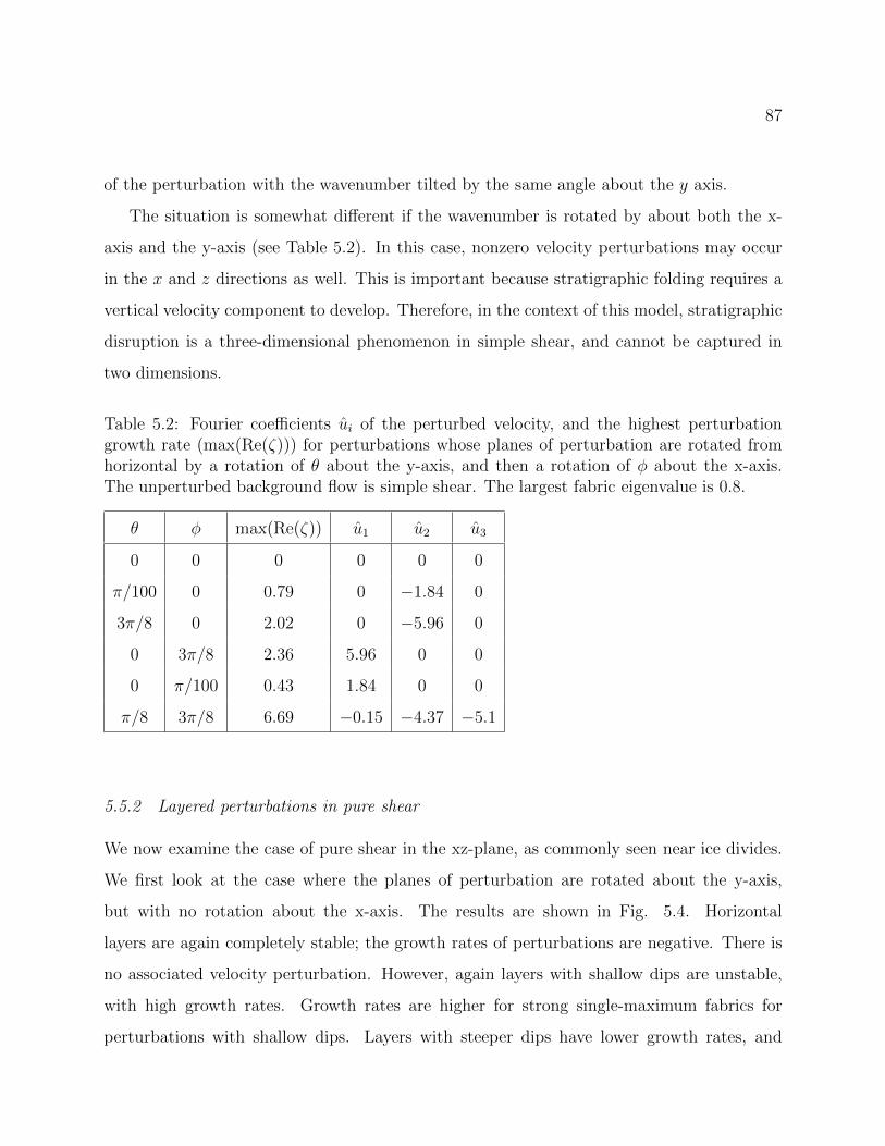
87
of the perturbation with the wavenumber tilted by the same angle about the y axis.
The situation is somewhat different if the wavenumber is rotated by about both the x-
axis and the y-axis (see Table 5.2). In this case, nonzero velocity perturbations may occur
in the x and z directions as well. This is important because stratigraphic folding requires a
vertical velocity component to develop. Therefore, in the context of this model, stratigraphic
disruption is a three-dimensional phenomenon in simple shear, and cannot be captured in
two dimensions.
Table 5.2: Fourier coefficients ui of the perturbed velocity, and the highest perturbationgrowth rate (max(Re(ζ))) for perturbations whose planes of perturbation are rotated fromhorizontal by a rotation of θ about the y-axis, and then a rotation of φ about the x-axis.The unperturbed background flow is simple shear. The largest fabric eigenvalue is 0.8.
θ φ max(Re(ζ)) u1 u2 u3
0 0 0 0 0 0
π/100 0 0.79 0 −1.84 0
3π/8 0 2.02 0 −5.96 0
0 3π/8 2.36 5.96 0 0
0 π/100 0.43 1.84 0 0
π/8 3π/8 6.69 −0.15 −4.37 −5.1
5.5.2 Layered perturbations in pure shear
We now examine the case of pure shear in the xz-plane, as commonly seen near ice divides.
We first look at the case where the planes of perturbation are rotated about the y-axis,
but with no rotation about the x-axis. The results are shown in Fig. 5.4. Horizontal
layers are again completely stable; the growth rates of perturbations are negative. There is
no associated velocity perturbation. However, again layers with shallow dips are unstable,
with high growth rates. Growth rates are higher for strong single-maximum fabrics for
perturbations with shallow dips. Layers with steeper dips have lower growth rates, and

88
Table 5.3: Fourier coefficients ui of the perturbed velocity, and the highest perturbationgrowth rate (max(Re(ζ))) for perturbations whose planes of perturbation are rotated fromhorizontal by a rotation of θ about the x-axis, and then a rotation of φ about the x-axis.The unperturbed background flow is pure shear. The largest fabric eigenvalue is 0.8.
θ φ max(Re(ζ)) u1 u2 u3
0 0 -0.4 0 0 0
π/100 0 1.08 0 0.53 −0.17
3π/8 0 3.13 0 0.794 −1.92
0 π/100 5.13 −2.36 0 −0.07
0 3π/8 15.81 −3.53 0 −8.54
π/8 3π/8 13.82 −3.54 0.83 −7.66
become stable for strong single-maximum fabrics. When the wavenumber is rotated about
the x-axis as well, fabrics become generally less stable.
The highest growth rates for perturbations whose wavevectors are rotated about the x-
axis are shown in Fig. 5.3. The results are similar to the case where the wavevector is rotated
about the x-axis (Figure 5.4), except the growth rates are generally higher. The growth rates
for more steeply-dipped perturbations are near zero for strong fabrics, but do not become
strongly negative.
In Table 5.3, the Fourier coefficients of velocity perturbations and maximum growth
rates are listed for perturbations whose wavevectors are rotated from vertical by several
combinations of angles φ (about the y-axis) and θ (about the x-axis). This table illustrates
that the wavevector must have a nonzero component in both x- and y-directions in order to
produce a nonzero velocity perturbation in all three directions.
5.5.3 Discussion
In the flow scenarios considered, dynamic instability seems to be the rule rather than the
exception. An important constraint to the flow perturbations is that the perturbed velocity

89
must be orthogonal to the wavevector, and parallel to the plane of the perturbations. This
can be seen from the incompressibility constraint (5.25) in the perturbation model, u ·κ = 0.
Since the velocity perturbation is εu cos(κ · x), this means that the velocity perturbation
must be orthogonal to the wavevector. Thus, if the wavevector is vertical, then there cannot
be a vertical component to the velocity perturbation. The perturbed velocity gradient must
consist solely of shear orthogonal to the wavevector.
To overturn stratigraphic layers in ice sheets, there must be a vertical velocity component.
This means that perturbations of horizontal layers can never generate vertical movement,
since the velocity perturbation is confined to the plane of perturbation. However, a layer
needs to be tilted only a small amount to produce a vertical-velocity perturbation, and fabric
perturbations on layers with shallow but nonzero dips tend to have higher growth rates. This
corresponds to “buckling.” Depending on the sign of cos(κ·x), this perturbation moves some
ice upwards, and other ice downwards. In flank flow, the perturbation must have a tilt in
both x and y to generate vertical motion.
Growth rates of perturbations in this model can be very high. However, it is important
to keep in mind some of the limitations of this model. It is applicable only to perturbations
with thicknesses sufficiently smaller than the ice sheet. For thick layers, the effects of the
ice-sheet boundaries become more important, violating the assumptions of this model. The
scale of perturbations must also be large enough that the ice can be treated as a continuum.
In addition, it is a first-order model, valid for small perturbations. As perturbations become
larger, higher-order effects (which this model does not capture) become important. However,
the stability of perturbations in this model can show in which situations perturbations can
develop in the first place.
Even with a high growth rate, a sufficiently-small initial perturbation could take quite
some time to grow large. For this reason, we do not expect large perturbations to develop in
upper layers of ice sheets. However, perturbations may have enough time to develop in the
lower layers of ice sheets. This may be especially true for flank flow, where simple shear dom-
inates. The high shear stress near the bed would accelerate the growth of the perturbations.

90
It is possible that the effects of coupled flow on perturbations, studied in this paper, may
reinforce the development of perturbations from other sources. Disturbed layering is ubiq-
uitous in deeper layers of ice sheets, and any flow disruption will also have a corresponding
effect on fabric. Disturbances due to basal topography, spatially-variable recrystallization,
or basal freeze-on may provide additional means of seeding fabric perturbations.
5.6 Conclusions
Due to the strong viscous anisotropy of ice as a function of c-axis orientation fabric, it is im-
portant to understand flow of anisotropic ice as a coupled system. To this end, we developed
a first-order coupled perturbation model of fabric evolution and flow of anisotropic ice. We
examined the stability of the system under various perturbations and flow scenarios. Under
this model, coupled ice flow and fabric evolution is unstable across a wide range of flow and
fabric conditions. Fabric perturbations are capable of causing vertical-velocity gradients for
both simple shear and pure shear. This is a potential mechanism for stratigraphic disruption
in ice. The instabilities would not occur in fabric that is uncoupled to flow. These types of
perturbations may help explain the small-scale stratigraphic disturbances seen far above the
bed in ice sheets. In addition, it provides a means of growth for fabric perturbations from
other sources.
Further numerical simulations of macroscopic coupled flow and fabric would shed more
light on the development of perturbations. The numerical model of coupled fabric and
plane flow in Gillet-Chaulet et al. [38] seems to show large fabric perturbations developing in
response to basal topography. Additional numerical simulations, especially three-dimensional
ones, in different flow scenarios, and with different initial fabric perturbations, would be
useful. The results from this analytical model suggest that two-dimensional flow models are
not capable of capturing the growth of perturbations in simple shear. This reinforces the
fact that flow of anisotropic ice and fabric development is a fundamentally three-dimensional
problem which cannot be represented as plane flow.

91
Chapter 6
CONCLUSIONS
6.1 Summary
Chapter 2 develops novel analytical and bootstrap estimates of the sampling error of fabric
eigenvalues and fabric eigenvectors. I showed that typically very uneven grain-size distri-
butions produce much larger uncertainties in area-weighted estimates of fabric properties.
I also applied bootstrapping to estimate the confidence intervals of the inferred strain en-
hancement factor in simple shear. Due to the power-law rheology of ice, I showed that the
enhancement factor is very poorly constrained by thin sections. I also introduced a new
parameterized orientation distribution function, the Bingham distribution, to glacioogy. I
compared the performance of this distribution to the Dinh-Armstrong distribution and the
Fisherian distribution proposed by Lliboutry. I showed that the Dinh-Armstrong distribu-
tion and the Bingham distribution produce much better fits than the Fisherian distribution.
This underscores the shortcomings of axially-symmetric distributions for representing most
realistic fabrics seen in ice cores.
Chapter 3 explores the use of sonic velocity measurements to infer ice fabric in boreholes,
with application to P-wave data taken from NEEM. I developed a model which estimates
eigenvalues in boreholes using both thin-section measurements and P, Sv, and Sh sonic
velocities. This model helps combine the relative strengths of the two measurement methods,
while reducing their relative weaknesses. Thin-section samples provide unbiased (although
possibly dependent) measurements of thin-section samples, but they have typically large
sampling error. Sonic velocity measurements, on the other hand, nearly eliminate sampling
error due to the large amount of ice sampled by the sound waves. However, model error can
be significant. In addition, poor tool centering was a problem at NEEM, which produced

92
large but fairly smooth biases in the measured velocity. The method uses thin-section derived
eigenvalues to correct for this bias, producing continuous, more accurate estimation of fabric
eigenvalues.
The next two chapters move from examining error in measurement of fabric characteris-
tics to looking at stability of ice crystal fabrics in response to flow or fabric perturbations.
The fourth chapter examined the response of fabrics to small flow perturbations. I showed
that under random velocity gradient perturbations, tilted-cone fabrics (where the largest
concentration is not vertical) can develop in simple shear and pure shear. This can produce
deformation in components other than the applied stress, and potentially induce stratigraphic
disruption.
The fifth chapter develops a first-order coupled model of anisotropic ice-flow and fabric
evolution. It is informative to treat fabric evolution and anisotropic flow as a coupled sys-
tem, since fabric greatly affects flow, and vice-versa. I applied this model to examine the
stability of spatially heterogeneous fabric perturbations in both simple shear and pure shear.
I showed that single-maximum fabrics in this coupled system are unstable. This has impor-
tant implications for the development of stratigraphic disruption in ice sheets. All unstable
perturbations in this model cause vertical offset in layers, which can invert stratigraphic
layers.
6.2 Implications
This thesis reinforces the utility of sonic measurements of fabric to avoid the severe sam-
pling error and spatial discontinuities of thin-section fabric measurements. Future work
incorporating S-waves will expand the usefulness of sonic method by allowing inference of in-
formation on azimuthal c-axis concentration. However, despite their inaccuracy, thin-section
fabric measurements can be effectively used in combination with sonic measurements.
This work underscores the difficulty of predicting ice-core fabrics and anisotropic ice-flow.
My work indicates that basal ice flow and fabric development may be nearly impossible to
predict accurately on smaller length scales at high strains, due to the instabilities of coupled

93
ice flow and fabric evolution. Further numerical investigations of coupled anisotropic ice-flow
and fabric evolution would be useful to expand on the analytical treatment in Chapter 5.
In particular, larger-scale perturbations which interact with the ice boundaries or temporal
flow perturbations could be investigated.
This thesis also lends support to the idea that fabric anisotropy may aid the development
of stratigraphic disturbances in basal ice. Stratigraphic disturbances are very commonly seen
in ice cores (e.g. Fuchs and Leuenberger [31]) Alley et al. [7]). Steeply dipping disturbed basal
layers are also a leading candidate for the cause of the abrupt loss of radar returns in echo-
free zones in Greenland and Antarctica [22]. Irregular bed topography alone cannot explain
stratigraphic disturbances. Temporal variations in flow over an irregular bed or significant
basal freeze-on can cause stratigraphic disruption. However, I speculate that interactions
of fabric with ice flow, sometimes in concert with temporal flow and bed topography, are
a better explanation of the seeming ubiquitousness of disturbed basal ice. Unlike temporal
flow or basal freeze-on, fabric exerts a strong influence on ice flow everywhere, which is not
necessarily true of these other processes.

94
.1 Appendix A: Derivation of analytical estimates of sampling error
We now derive analytical estimates for sampling error from estimating the bulk second-order
orientation tensor from ice core thin sections. First, we focus on the case of per-pixel EBSD
or automatic fabric analyzer measurements, which typically yield many measurements per
grain. We take into account correlations between different measurements. It is important
to take depedendence between measurements into account in this case. Samples taken from
the same grain will be highly correlated, since intragranular misorientations are typically no
more than a few degrees.
In this section, upper indices represent spatial locations, and lower indices are indices for
tensor quantities at one location. For example, cki is the i component of the c-axis tensor at
spatial location k. Let Aij =∑
k akij/N be the sample estimate of Aij, where akij = cki c
kj (no
sum in k) is a component of the structure tensor for an individual c-axis measurement, and N
is the total number of measurements. We assume that each measurement is equally weighted,
for simplicity of presentation. Extending these results to the case where measurements are
not equally weighted is fairly simple.
Suppose that we can determine a covariance tensor giving the covariance between the ij
component of the structure tensors at spatial locations k and l. This is given by,
Cklij = Cov(akij, a
lij). (1)
Now, we wish to determine the variance of the sample estimate Aij. First, note that
Var(akij/N) = Var(akij)/N2. Also, the variance of a sum of random variables X1, ..., Xn
is,
Var
(∑i
Xi
)=∑i,j
Cov(Xi, Xj) (2)

95
Since Aij =∑
k akij/N , we have,
Var(Aij) = Var
(∑k
akijN
)(3)
=∑k,l
Cklij
N2(4)
where Cklij is the covariance between the structure tensor akij at site k and alij at site l, and
N is the total number of measurements in the thin section. From the previous equation,
we can see that if each structure-tensor measurement is strongly correlated with m other
measurements, then the variance of Aij would be approximately m times larger than if it
were uncorrelated. In a high-resolution per-pixel thin-section measurement, a single pixel
can be expected to be highly correlated with many other pixels.
The structure tensor akij for measurement k can be written as the sum
akij = Aij + gkij + hkij. (5)
Here, gkij is a random component accounting for intergrain variance in akij, constant across
each grain. Let the site k be in grain M . Then, gkij = aMij − Aij, where the mean aMij is
the expectation of alij taken over all measurements l in grain M . Likewise, hkij is a random
component which can be identified with intragrain variability. By rearranging terms, hkij =
akij − Aij − gkij. We assume that gkij and hkij are independent.
Note that we separate out the mean of Aij, which is the mean of akij (for all k) taken
over the ODF. Furthermore, we are also separating out the mean of each individual grain as
well. This decomposition separates out the components of the structure tensor that vary on
different length scales: global (Aij), per grain (gkij), and intragrain (hkij). This will allow us
look at the relative contributions of these components, and their effect on sampling error.
Suppose akij and alij were taken from the same grain. Let Gklij be the covariance between
gkij and glij. From Equation (5), gkij = glij. This also implies that every entry of the covariance
tensor of gkij, Gklij , is equal to Cov(gkij, g
lij) = Var(gkij) (no sum), for all k, l taken from the

96
same grain. Due to independence between gkij and hkij, we can write the covariance as the
sum Cklij = Hkl
ij +Gklij , where Hkl
ij is the covariance between hkij and hlij.
Correlation between adjacent grains is usually small, unless there is active polygonization
[26]. Correlation between distant grains is always small, even if two distant grains happen
to have similar orientations. Therefore, we are justified in neglecting covariances between
points in different grains. This means that we can take Gklij = 0 and Hkl
ij = 0 whenever
observations k and l are not from the same grain.
We now show that the intragrain variability, hkij, may be ignored under some light as-
sumptions. The covariance Hklij is non-negligible only where points k and l lie not only within
the same grain (otherwise it is zero by assumption), but sufficiently close together. This is
because intragraular misorientations, for example due to the formation of subgrain bound-
aries, occur on lengths smaller than the grain. Because of this, Hklij is negligible for may
more combinations of k and l than Gklij is. In addition, intragranular c-axis misorientations
are usually not more than a few degrees, so the covariance (as opposed to correlation) Hklij is
likely small for even highly correlated nearby pairs of c-axis measurements k, l. Given this,
we may approximate the total covariance Cklij ≈ Gkl
ij .
This implies that Cklij = Cpq
ij ≈ Gklij = Var(gkij) ≈ Var(cki c
kj ), whenever k, l, p, q lie in the
same grain, and zero otherwise. From this, we can write the variance of the sum of all akij
taken from a grain m as nmVar(cmi cmi ), where nm is the number of observations from the grain
with index m. Finally, due to independence between different grains, Var(cmi cmj ) = Var(cicj)
is the same for all grains, since by these assumptions they are drawn independently from the
same ODF.
Now we have an expression for the variance of individual grains in terms of Var(cicj).
Then, we can write Var(Aij) as a sum of the variances of individual grains, in turn. This is
given by,
Var(Aij) ≈∑m
(wm)2Var(cicj) = s2nVar(cicj) (6)
where wm = nm/N is a weighting coefficient corresponding to the fraction of observations

97
lying in grain m of a total number of observations N . The coefficient s2n is the sum of
the squared weights. If we have many observations per grain, Equation (6) substantially
simplifies treatment of uncertainty compared to Equation (3). By only considering data
on a per-grain basis and ignoring intragrain c-axis variability, we are also able to use the
same analysis for thin-section data collected per-grain (as in the Rigsby Stage method), or
per-pixel (as with EBSD or automatic fabric analyzers). Note that in the case of c-axis
measurements given per-grain, rather than per-pixel, weighting the measurements by grain
area is physically preferred to equal weighting [35]. Area weighting also yields similar variance
estimates to per-pixel measurements, if the number of per-pixel measurements in each grain
is proportional to the area.
We now derive analytical estimates of the distribution of the sample estimate Aij, using
Equation (6). For a large-enough sample, Aij will have principal directions and eigenvalues
close to those of Aij. For a large enough number of grains, we can apply the central limit
theorem to estimate the sampling distribution of Aij. As the number of sampled grains n
becomes large, Aij converges in distribution to the normal distribution with mean Aij and
variance Var(cicj)s2n.
Variance is the mean of the square minus the square of the mean. From this, Var(cicj) =<
cicjcicj > − < cicj >2= Aijij − AijAij. Then, the variance of the sample estimate of Aij is
given by,
Var(Aij) ≈ (Aijij − AijAij) s2n (7)
≈(Aijij − AijAij
)s2n (8)
with no sum in i or j. The preceding gives us an expression for variance of the sample estimate
Aij of Aij. Note that s2n is at a minimum when all area weights are equal, corresponding
to equal grain weighting. In that case, the sum of squared weights is s2n = n−1. This is
the minimum s2n for any choice of positive weightings that sum to unity. Therefore, equal
weighting of grains always underestimates sampling error.
For simplicity, we choose to work in the reference frame defined by the three true fabric

98
eigenvectors. In this case, Aij is a diagonal matrix of the fabric eigenvalues λi, and the
components of ci are uncorrelated. For a large enough number of grains, Aij = Aij + εij,
where εij is small. We can then estimate the sampled fabric eigenvalues and eigenvectors as a
first-order perturbation of the original eigenvalues and eigenvectors. In this case, let Aij have
eigenvalues λi = Aii (no sum). Also, let the fabric sample have eigenvalues λi = λi + δλi.
Then, to first order, δλi = εii (no sum) [78].
It follows that the variance of sample eigenvalues λi is then given by Var(Aii) (no sum),
since Aii = λi (no sum). This is most easily found by calculating Var(c2i ), where ci is expressed
in the reference frame defined by the principal directions, and has zero empirical mean. In the
case of analytical orientation distribution functions, the second- and fourth-order orientation
tensors, which correspond to the second and fourth moments of the distribution, can be used
directly. From this, it can be seen that samples from more diffuse orientation distribution
functions will have larger variance of sample eigenvalues, and concentrated fabrics will have
less variance.
Now that we have an estimate for the sample variance of eigenvalue estimates from thin
sections, we examine sampling error of the fabric eigenvectors, or principal directions. Sim-
ilarly to the eigenvalues, we use a first-order approximation of the eigenvalue perturbations
[78]. If we are in the reference frame defined by the true fabric eigenvectors, then the sam-
ple estimate A will be be close to being diagonal, with small off-diagonal elements. The
eigenvalues V of the A are then,
V =
1 A12
λ2−λ1A13
λ3−λ1A21
λ1−λ2 1 A23
λ3−λ2A31
λ1−λ3A12
λ2−λ3 1
, (9)
to first-order accuracy in Aij. The perturbed eigenvalue matrix V is then also an infinitesimal
rotation matrix, which is a first-order approximation for rotation matrices valid for small
rotation angles. This defines the approximate reference frame formed by the perturbed
eigenvectors. The three elements above the diagonal are the Euler angles of this infinitesimal

99
rotation, with α = V23, β = V13, and γ = V12 being the rotation angles around the z-axis,
y-axis, and x-axis, respectively. As before, the sample-based estimate Aij of the component
of the second-order orientation tensor Aij is approximately normally distributed for a large
enough sample of grains, with variance (Aijij−AijAij)s2n (no sum). Thus, α is approximately
normally distributed with variance (λ2 − λ1)−2Var(A12), and a mean of zero. The cases for
β and γ are similar.
From this, variance of the Euler angle about an axis is inversely proportional to the
difference in the fabric eigenvalues associated with the other two axes. This means that the
variance becomes large if the other two eigenvalues are very close together. It is not defined
if the eigenvalues are identical. This is because if there are two identical eigenvalues, then
there are two corresponding orthogonal eigenvectors, and any vector in the plane formed by
those eigenvectors is an eigenvector. Therefore, there is not a unique reference frame which
makes A diagonal in this case.
Grain-size distribution also has an important influence on sampling error of eigenvalue and
eigenvector estimates. Uneven distributions, in which a small number of large grains account
for most of the volume, induce greater sampling uncertainty than a grain-size distribution of
more evenly-sized grains. As an extreme example, if a fabric thin section contains one large
grain, and a thousand infinitesimally small grains, the sample size is effectively one grain,
because the small grains have weightings close to zero. The variance of Aij is proportional to
the sum of squared weights, s2n. This attains a minimum value for equal weights. Grain-size
distributions found in ice cores often have a few large grains and many small grains. Equal
weighting can therefore lead to a significant underestimate of sampling error.

100
BIBLIOGRAPHY
[1] M. Abadi, A. Agarwal, P. Barham, E. Brevdo, Z. Chen, C. Citro, G.S. Corrado,
A. Davis, J. Dean, M. Devin, et al. Tensorflow: Large-scale machine learning on het-
erogeneous distributed systems. arXiv preprint arXiv:1603.04467, 2016.
[2] S.G. Advani and C.L. Tucker. The use of tensors to describe and predict fiber orientation
in short fiber composites. Journal of Rheology (1978-present), 31(8):751–784, 1987.
[3] S.G. Advani and C.L Tucker. Closure approximations for three-dimensional structure
tensors. Journal of Rheology, 34(3):367–386, 1990.
[4] K. Aki and P.G. Richards. Quantitative Seismology: Theory and Methods. WH Freeman
and Company, San Francisco, 1980.
[5] R.B. Alley. Fabrics in polar ice sheets: development and prediction. Science, 240(4851):
493, 1988.
[6] R.B. Alley. Flow-law hypotheses for ice-sheet modeling. J. Glaciol, 38(129):245–256,
1992.
[7] R.B. Alley, A.J. Gow, D.A. Meese, J.J. Fitzpatrick, E.D. Waddington, and J.F. Bolzan.
Grain-scale processes, folding, and stratigraphic disturbance in the GISP2 ice core.
Journal of Geophysical Research, 102(C12):26819–26, 1997.
[8] N. Azuma. A flow law for anisotropic ice and its application to ice sheets. Earth and
Planetary Science Letters, 128(3-4):601–614, 1994.
[9] N Azuma. A flow law for anisotropic polycrystalline ice under uniaxial compressive
deformation. Cold regions science and technology, 23(2):137–147, 1995.

101
[10] N. Azuma and K. Goto-Azuma. An anisotropic flow law for ice-sheet ice and its impli-
cations. Annals of Glaciology, 23:202–208, 1996.
[11] R.E. Bell, K. Tinto, I. Das, M. Wolovick, W. Chu, T.T. Creyts, N. Frearson, A. Abdi,
and J.D. Paden. Deformation, warming and softening of greenland’s ice by refreezing
meltwater. Nature Geoscience, 7(7):497–502, 2014.
[12] C.R. Bentley. Seismic-wave velocities in anisotropic ice: A comparison of measured and
calculated values in and around the deep drill hole at Byrd Station, Antarctica. Journal
of Geophysical Research, 77(23):4406–4420, 1972.
[13] C. Bingham. An antipodally symmetric distribution on the sphere. The Annals of
Statistics, pages 1201–1225, 1974.
[14] G. Bouchard. Efficient bounds for the softmax function and applications to approximate
inference in hybrid models. In NIPS 2007 workshop for approximate Bayesian inference
in continuous/hybrid systems, 2007.
[15] O. Castelnau, G.R. Canova, R.A. Lebensohn, and P. Duval. Modelling viscoplastic be-
havior of anisotropic polycrystalline ice with a self-consistent approach. Acta materialia,
45(11):4823–4834, 1997.
[16] D.H. Chung and T.H. Kwon. Invariant-based optimal fitting closure approximation for
the numerical prediction of flow-induced fiber orientation. Journal of rheology, 46(1):
169–194, 2002.
[17] N. Cressie. Statistics for spatial data: Wiley series in probability and statistics. Wiley-
Interscience New York, 15:16, 1993.
[18] K.M. Cuffey, Th. Thorsteinsson, and E.D. Waddington. A renewed argument for crystal
size control of ice sheet strain rates. Journal of Geophysical Research: Solid Earth, 105
(B12):27889–27894, 2000.

102
[19] A. Diez and O. Eisen. Seismic wave propagation in anisotropic ice-part 1: Elasticity
tensor and derived quantities from ice-core properties. The Cryosphere, 9(1):367–384,
2015.
[20] S. Dinh and R. Armstrong. A rheological equation of state for semiconcentrated fiber
suspensions. Journal of Rheology (1978-present), 28(3):207–227, 1984.
[21] C.L. DiPrinzio, L.A. Wilen, R.B. Alley, J.J. Fitzpatrick, M.K. Spencer, and A.J. Gow.
Fabric and texture at Siple Dome, Antarctica. Journal of Glaciology, 51(173):281–290,
2005.
[22] R. Drews, O. Eisen, I. Weikusat, S. Kipfstuhl, A. Lambrecht, D. Steinhage, F. Wilhelms,
and H. Miller. Layer disturbances and the radio-echo free zone in ice sheets. The
Cryosphere, 3(2):195–203, 2009.
[23] J. Duchi and Y. Hazan, E.and Singer. Adaptive subgradient methods for online learning
and stochastic optimization. Journal of Machine Learning Research, 12(Jul):2121–2159,
2011.
[24] G. Durand, O. Gagliardini, T. Thorsteinsson, A. Svensson, S. Kipfstuhl, and D. Dahl-
Jensen. Ice microstructure and fabric: an up-to-date approach for measuring textures.
Journal of Glaciology, 52(179):619–630, 2006.
[25] G. Durand, F. Gillet-Chaulet, A. Svensson, O. Gagliardini, S. Kipfstuhl, J. Meyssonnier,
F. Parrenin, P. Duval, D. Dahl-Jensen, et al. Change in ice rheology during climate
variations–implications for ice flow modelling and dating of the EPICA Dome C core.
Climate of the Past, 3(1):155–167, 2007.
[26] G. Durand, A. Persson, D. Samyn, and A. Svensson. Relation between neighbouring
grains in the upper part of the northgrip ice core - implications for rotation recrystal-
lization. Earth and planetary science letters, 265(3):666–671, 2008.

103
[27] G. Durand, A. Svensson, A. Persson, O. Gagliardini, F. Gillet-Chaulet, J. Sjolte,
M. Montagnat, and D. Dahl-Jensen. Evolution of the texture along the EPICA Dome
C ice core. Low Temperature Science, 68(Supplement):91–105, 2009.
[28] P. Duval, MF Ashby, and I. Anderman. Rate-controlling processes in the creep of
polycrystalline ice. The Journal of Physical Chemistry, 87(21):4066–4074, 1983.
[29] B. Efron. Bootstrap methods: another look at the jackknife. Springer, 1992.
[30] J. Fitzpatrick, D. Voigt, J. Fegyveresi, N. Stevens, M. Spencer, J. Cole-Dai, R. Alley,
G. Jardine, E. Cravens, L. Wilen, et al. Physical properties of the WAIS Divide ice
core. Journal of Glaciology, 60(224):1181, 2014.
[31] A. Fuchs and M.C. Leuenberger. δ18o of atmospheric oxygen measured on the grip ice
core document stratigraphic disturbances in the lowest 10% of the core. Geophysical
Research Letters, 23(9):1049–1052, 1996.
[32] T.J. Fudge, K.C. Taylor, E.D. Waddington, J.J. Fitzpatrick, and H. Conway. Electrical
stratigraphy of the WAIS Divide ice core: Identification of centimeter-scale irregular
layering. Journal of Geophysical Research: Earth Surface, 121(7):1218–1229, 2016.
[33] O. Gagliardini and J. Meyssonnier. Plane flow of an ice sheet exhibiting strain-induced
anisotropy. In Advances in cold-region thermal engineering and sciences, pages 171–182.
Springer, 1999.
[34] O. Gagliardini, G. Durand, and Y. Wang. Grain area as a statistical weight for poly-
crystal constituents. Journal of Glaciology, 50(168):87–95, 2004.
[35] O. Gagliardini, G. Durand, and Y. Wang. Grain area as a statistical weight for poly-
crystal constituents. Journal of Glaciology, 50(168):87–95, 2004.

104
[36] O. Gagliardini, F. Gillet-Chaulet, and M. Montagnat. A review of anisotropic po-
lar ice models: from crystal to ice-sheet flow models. Low Temperature Science, 68
(Supplement):149–166, 2009.
[37] F. Gillet-Chaulet, O. Gagliardini, J. Meyssonnier, M. Montagnat, and O. Castelnau. A
user-friendly anisotropic flow law for ice-sheet modelling. Journal of glaciology, 51(172):
3–14, 2005.
[38] F. Gillet-Chaulet, O. Gagliardini, J. Meyssonnier, T. Zwinger, and J. Ruokolainen.
Flow-induced anisotropy in polar ice and related ice-sheet flow modelling. Journal of
Non-Newtonian Fluid Mechanics, 134(1):33–43, 2006.
[39] John W Glen. The creep of polycrystalline ice. In Proceedings of the Royal Society of
London A: Mathematical, Physical and Engineering Sciences, volume 228, pages 519–
538. The Royal Society, 1955.
[40] G. Godert. A mesoscopic approach for modelling texture evolution of polar ice including
recrystallization phenomena. Annals of Glaciology, 37(1):23–28, 2003.
[41] G. Godert and K. Hutter. Induced anisotropy in large ice shields: theory and its
homogenization. Continuum Mechanics and Thermodynamics, 10(5):293–318, 1998.
[42] A. Gusmeroli, E.C. Pettit, J.H. Kennedy, and C. Ritz. The crystal fabric of ice from
full-waveform borehole sonic logging. Journal of Geophysical Research: Earth Surface,
117(F3), 2012.
[43] P. Hall, J. Horowitz, and B. Jing. On blocking rules for the bootstrap with dependent
data. Biometrika, 82(3):561–574, 1995.
[44] M.B. Helgerud, W.F. Waite, S.H. Kirby, and A. Nur. Elastic wave speeds and moduli
in polycrystalline ice ih, si methane hydrate, and sii methane-ethane hydrate. Journal
of Geophysical Research: Solid Earth, 114(B2), 2009.

105
[45] R. Hill. The elastic behaviour of a crystalline aggregate. Proceedings of the Physical
Society. Section A, 65(5):349, 1952.
[46] D. Iliescu, I. Baker, and H. Chang. Determining the orientations of ice crystals using
electron backscatter patterns. Microscopy research and technique, 63(4):183–187, 2004.
[47] D. Jansen, M. Llorens, J. Westhoff, F. Steinbach, S. Kipfstuhl, P.D. Bons, A. Griera,
and I. Weikusat. Small-scale disturbances in the stratigraphy of the NEEM ice core:
observations and numerical model simulations. The Cryosphere, 10:359–370, 2016.
[48] G.B. Jeffery. The motion of ellipsoidal particles immersed in a viscous fluid. Proceedings
of the Royal Society of London. Series A, Containing papers of a mathematical and
physical character, pages 161–179, 1922.
[49] J. Kennedy, E. Pettit, and C. Di Prinzio. The evolution of crystal fabric in ice sheets
and its link to climate history. Journal of Glaciology, 59(214):357–373, 2013.
[50] D. Kluskiewicz, E.D. Waddington, S. Anandakrishnan, D.E. Voigt, K. Matsuoka, and
M.P. McCarthy. Sonic methods for measuring crystal orientation fabric in ice, and
results from the west antarctica ice sheet divide. 2017.
[51] C. Langway. Ice fabrics and the universal stage. Department of Defense, Department of
the Army, Corps of Engineers, Snow Ice and Permafrost Research Establishment, 1959.
[52] R.A. Lebensohn and C.N. Tome. A self-consistent anisotropic approach for the simu-
lation of plastic deformation and texture development of polycrystals: application to
zirconium alloys. Acta Metallurgica et Materialia, 41(9):2611–2624, 1993.
[53] R.C. Lile. The effect of anisotropy on the creep of polycrystalline ice. Journal of
Glaciology, 21(85):475–483, 1978.
[54] L. Lliboutry. Anisotropic, transversely isotropic nonlinear viscosity of rock ice and

106
rheological parameters inferred from homogenization. International journal of plasticity,
9(5):619–632, 1993.
[55] K. Mardia. Characterizations of directional distributions. In A Modern Course on
Statistical Distributions in Scientific Work, pages 365–385. Springer, 1975.
[56] A. Maurel, F. Lund, and M. Montagnat. Propagation of elastic waves through textured
polycrystals: application to ice. In Proc. R. Soc. A, volume 471, page 20140988. The
Royal Society, 2015.
[57] A. Maurel, J. Mercier, and M. Montagnat. Critical investigation of calculation methods
for the elastic velocities in anisotropic ice polycrystals. The Cryosphere, 10(6):3063–
3070, 2016.
[58] J. Meyssonnier and A. Philip. A model for the tangent viscous behaviour of anisotropic
polar ice. Annals of Glaciology, 23:253–261, 1996.
[59] M. Montagnat and P. Duval. Rate controlling processes in the creep of polar ice, influ-
ence of grain boundary migration associated with recrystallization. Earth and Planetary
Science Letters, 183(1):179–186, 2000.
[60] M. Montagnat, N. Azuma, D. Dahl-Jensen, J. Eichler, S. Fujita, F. Gillet-Chaulet,
S. Kipfstuhl, D. Samyn, A. Svensson, and I. Weikusat. Fabric along the NEEM ice core,
Greenland, and its comparison with GRIP and NGRIP ice cores. 2014.
[61] M. Montagnat, N. Azuma, D. Dahl-Jensen, J. Eichler, S. Fujita, F. Gillet-Chaulet,
S. Kipfstuhl, D. Samyn, A. Svensson, and I. Weikusat. Fabric along the NEEM ice core,
Greenland, and its comparison with GRIP and NGRIP ice cores. 2014.
[62] S. Montgomery-Smith. Perturbations of the coupled Jeffery-Stokes equations. Journal
of Fluid Mechanics, 681:622–638, 2011.

107
[63] S. Montgomery-Smith, W. He, D.A. Jack, and D.E. Smith. Exact tensor closures for the
three-dimensional Jeffery’s equation. Journal of Fluid Mechanics, 680:321–335, 2011.
[64] T. C. Onstott. Application of the Bingham distribution function in paleomagnetic
studies. Journal of Geophysical Research: Solid Earth, 85(B3):1500–1510, 1980.
[65] V.F. Petrenko and R.W. Whitworth. Physics of ice. OUP Oxford, 1999.
[66] A. Philip and J. Meyssonnier. Anisotropic isothermal ice-cap flow with the shallow ice
approximation. In Advances in Cold-Region Thermal Engineering and Sciences, pages
237–248. Springer, 1999.
[67] L. Placidi, R. Greve, H. Seddik, and S.H. Faria. Continuum-mechanical, anisotropic flow
model for polar ice masses, based on an anisotropic flow enhancement factor. Continuum
Mechanics and Thermodynamics, 22(3):221–237, 2010.
[68] C.E. Rasmussen. Gaussian processes for machine learning. 2006.
[69] G. Sachs. Zur ableitung einer fliebedingung. Z. Vereins Dtsch. Ing., 12(8):734–736,
1928.
[70] I.H. Sloan and R.S. Womersley. Extremal systems of points and numerical integration
on the sphere. Advances in Computational Mathematics, 21(1-2):107–125, 2004.
[71] E.C. Smith, A.F. Baird, J.M. Kendall, C. Martın, R.S. White, A.M. Brisbourne, and
A.M. Smith. Ice fabric in an antarctic ice stream interpreted from seismic anisotropy.
Geophysical Research Letters, 2017.
[72] R. Staroszczyk and O. Gagliardini. Two orthotropic models for strain-induced
anisotropy of polar ice. Journal of Glaciology, 45(151):485–494, 1999.
[73] B. Svendsem and K. Hutter. A continuum approach for modelling induced anisotropy
in glaciers and ice sheets. Annals of Glaciology, 23(1):262–269, 1996.

108
[74] G.I. Taylor. Analysis of plastic strain in a cubic crystal. Stephen Timoshenko 60th
Anniversary Volume, pages 218–224, 1938.
[75] T. Thorsteinsson. Fabric development with nearest-neighbor interaction and dynamic
recrystallization. J. Geophys. Res, 107(2014):10–1019, 2002.
[76] T. Thorsteinsson and E.D. Waddington. Folding in strongly anisotropic layers near
ice-sheet centers. Annals of Glaciology, 35(1):480–486, 2002.
[77] Throstur Thorsteinsson. Anisotropy of ice Ih: Development of fabric and effects of
anisotropy on deformation. PhD thesis, University of Washington, 2000.
[78] L. N. Trefethen and D. Bau III. Numerical linear algebra, volume 50. Siam, 1997.
[79] C. Vogt, K. Laihem, and C. Wiebusch. Speed of sound in bubble-free ice. The Journal
of the Acoustical Society of America, 124(6):3613–3618, 2008.
[80] R. Von Mises. Mechanics of plastic deformation of crystals. Applied Mathematics and
Mechanics, 592:8, 1928.
[81] J. Weertman. Creep deformation of ice. Annual Review of Earth and Planetary Sciences,
11(1):215–240, 1983.
[82] L Wilen. Ice Fabric Characteristics: Siple Dome, A Core. Boulder, CO: National Snow
and Ice Data Center, 2002. URL https://nsidc.org/data/nsidc-0255.
[83] L. A. Wilen, C. L. Diprinzio, R. B. Alley, and N. Azuma. Development, principles, and
applications of automated ice fabric analyzers. Microscopy research and technique, 62
(1):2–18, 2003.
[84] Q. Zheng and W. Zou. Orientation distribution functions for microstructures of hetero-
geneous materials (i) directional distribution functions and irreducible tensors. Applied
Mathematics and Mechanics, 22(8):865–884, 2001.