Embed Size (px)
Citation preview

Stability, Multiplicity, and Sunspots(deriving solutions to linearized system
&Blanchard-Kahn conditions)
Wouter J. Den HaanLondon School of Economics
c© by Wouter J. Den Haan

Multiplicity Getting started General Derivation Examples Time iteration and linear solutions
Content
1 A lot on sunspots
2 A simple way to get policy rules in a linearized framework
• and an even simpler way based on time iteration(an idea of Pontus Rendahl)
2 / 54

Multiplicity Getting started General Derivation Examples Time iteration and linear solutions
Introduction
• What do we mean with non-unique solutions?• multiple solution versus multiple steady states
• What are sunspots?• Are models with sunspots scientific?
3 / 54

Multiplicity Getting started General Derivation Examples Time iteration and linear solutions
Terminology
• Definitions are very clear• (use in practice can be sloppy)
Model:
H(p+1, p) = 0
Solution:p+1 = f (p)
4 / 54

Multiplicity Getting started General Derivation Examples Time iteration and linear solutions
Unique solution & multiple steady states
0 0.2 0.4 0.6 0.8 1 1.2 1.4 1.60
0.5
1
1.5
2
p
p+1
45o
5 / 54

Multiplicity Getting started General Derivation Examples Time iteration and linear solutions
Multiple solutions & unique (non-zero) steady state
0 0.2 0.4 0.6 0.8 1 1.2 1.4 1.6 1.8 20
0.2
0.4
0.6
0.8
1
1.2
1.4
1.6
1.8
2
p
p +1
45o
6 / 54

Multiplicity Getting started General Derivation Examples Time iteration and linear solutions
Multiple steady states & sometimes multiple solutions
34
“Traditional” Pic
ut
ut+1
45o
positive expectations
negative expectations
From Den Haan (2007)7 / 54

Multiplicity Getting started General Derivation Examples Time iteration and linear solutions
Large sunspots (around 2000 at the peak)
8 / 54

Multiplicity Getting started General Derivation Examples Time iteration and linear solutions
Past Sun Spot Cycles
Sun spots even had a "Great Moderation"9 / 54

Multiplicity Getting started General Derivation Examples Time iteration and linear solutions
Current cycle (at peak again)
10 / 54

Multiplicity Getting started General Derivation Examples Time iteration and linear solutions
Cute NASA video
• https://www.youtube.com/watch?v=UD5VViT08ME
11 / 54

Multiplicity Getting started General Derivation Examples Time iteration and linear solutions
Sunspots in economics
• Definition: a solution is a sunspot solution if it depends on astochastic variable from outside system
• Model:
0 = EH(pt+1, pt, dt+1, dt)
dt : exogenous random variable
12 / 54

Multiplicity Getting started General Derivation Examples Time iteration and linear solutions
Sunspots in economics (Cass & Shell 1983)
• Non-sunspot solution:
pt = f (pt−1, pt−2, · · · , dt, dt−1, · · · )
• Sunspot:
pt = f (pt−1, pt−2, · · · , dt, dt−1, · · · , st)
st : random variable with E [st+1] = 0
13 / 54

Multiplicity Getting started General Derivation Examples Time iteration and linear solutions
Origin of sunspots in economics
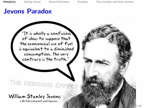
• William Stanley Jevons (1835-82) explored empiricalrelationship between sunspot activity (that is, the real thing!!!)and the price of corn.
• Fortunately, Jevons had some other contributions as well, suchas "Jevons Paradox". His work is considered to be the start ofmathematical economics.
14 / 54
Multiplicity Getting started General Derivation Examples Time iteration and linear solutions
Jevons Paradox
15 / 54

Multiplicity Getting started General Derivation Examples Time iteration and linear solutions
Sunspots and science
Why are sunspots attractive
• sunspots: st matters, just because agents believe this
• self-fulfilling expectations don’t seem that unreasonable
• sunspots provide many sources of shocks• number of sizable fundamental shocks small
16 / 54

Multiplicity Getting started General Derivation Examples Time iteration and linear solutions
Sunspots and science
Why are sunspots not so attractive
• Purpose of science is to come up with predictions• If there is one sunspot solution, there are zillion others as well
• Support for the conditions that make them happen notoverwhelming
• you need suffi ciently large increasing returns to scale orexternality
17 / 54

Multiplicity Getting started General Derivation Examples Time iteration and linear solutions
Overview
1 Getting started
• simple examples
2 General derivation of Blanchard-Kahn solution
• When unique solution?• When multiple solution?• When no (stable) solution?
3 When do sunspots occur?
4 Numerical algorithms and sunspots
18 / 54

Multiplicity Getting started General Derivation Examples Time iteration and linear solutions
Getting started
•Model: yt = ρyt−1
• infinite number of solutions, independent of the value of ρ
19 / 54

Multiplicity Getting started General Derivation Examples Time iteration and linear solutions
Getting started
•Model: yt = ρyt−1
• infinite number of solutions, independent of the value of ρ
19 / 54

Multiplicity Getting started General Derivation Examples Time iteration and linear solutions
Getting started
•Model: yt+1 = ρyt
y0 is given
• unique solution, independent of the value of ρ
20 / 54

Multiplicity Getting started General Derivation Examples Time iteration and linear solutions
Getting started
•Model: yt+1 = ρyt
y0 is given
• unique solution, independent of the value of ρ
20 / 54

Multiplicity Getting started General Derivation Examples Time iteration and linear solutions
Getting started
• Blanchard-Kahn conditions apply to models that add as arequirement that the series do not explode
yt+1 = ρytModel:
yt cannot explode
• ρ > 1: unique solution, namely yt = 0 for all t• ρ < 1: many solutions• ρ = 1: many solutions
• be careful with ρ = 1, uncertainty matters
21 / 54

Multiplicity Getting started General Derivation Examples Time iteration and linear solutions
State-space representation
Ayt+1 + Byt = εt+1
E [εt+1|It] = 0
yt : is an n× 1 vectorm ≤ n elements are not determined
some elements of εt+1 are not exogenous shocks but prediction errors
22 / 54

Multiplicity Getting started General Derivation Examples Time iteration and linear solutions
Neoclassical growth model and state space representation
(exp(zt)kα
t−1 + (1− δ)kt−1 − kt)−γ
=
E
[β (exp(zt+1)kα
t + (1− δ)kt − kt+1)−γ
×(
α exp (zt+1) kα−1t + 1− δ
) ∣∣∣∣∣ It
]
or equivalently without E [·](exp(zt)kα
t−1 + (1− δ)kt−1 − kt)−γ
=
β (exp(zt+1)kαt + (1− δ)kt − kt+1)
−γ
×(
α exp (zt+1) kα−1t + 1− δ
)+eE,t+1
23 / 54
Multiplicity Getting started General Derivation Examples Time iteration and linear solutions
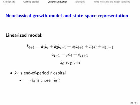
Neoclassical growth model and state space representation
Linearized model:
kt+1 = a1kt + a2kt−1 + a3zt+1 + a4zt + eE,t+1
zt+1 = ρzt + ez,t+1
k0 is given
• kt is end-of-period t capital• =⇒ kt is chosen in t
24 / 54

Multiplicity Getting started General Derivation Examples Time iteration and linear solutions
Neoclassical growth model and state space representation
1 0 -a30 1 00 0 1
kt+1kt
zt+1
+ -a1 -a2 -a4-1 0 00 0 -ρ
ktkt−1
zt
= eE,t+1
0ez,t+1
25 / 54

Multiplicity Getting started General Derivation Examples Time iteration and linear solutions
Dynamics of the state-space system
Ayt+1 + Byt = εt+1
yt+1 = −A−1Byt +A−1εt+1
= Dyt +A−1εt+1
Thus
yt+1 = Dty1 +t
∑l=1
Dt−lA−1εl+1
26 / 54
Multiplicity Getting started General Derivation Examples Time iteration and linear solutions
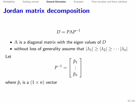
Jordan matrix decomposition
D = PΛP−1
• Λ is a diagonal matrix with the eigen values of D• without loss of generality assume that |λ1| ≥ |λ2| ≥ · · · |λn|
Let
P−1 =
p̃1...
p̃n
where p̃i is a (1× n) vector
27 / 54

Multiplicity Getting started General Derivation Examples Time iteration and linear solutions
Dynamics of the state-space system
yt+1 = Dty1 +t
∑l=1
Dt−lA−1εl+1
= PΛtP−1y1 +t
∑l=1
PΛt−lP−1A−1εl+1
28 / 54

Multiplicity Getting started General Derivation Examples Time iteration and linear solutions
Dynamics of the state-space system
multiplying dynamic state-space system with P−1 gives
P−1yt+1 = ΛtP−1y1 +t
∑l=1
Λt−lP−1A−1εl+1
or
p̃iyt+1 = λti p̃iy1 +
t
∑l=1
λt−li p̃iA−1εl+1
recall that yt is n× 1 and p̃i is 1× n. Thus, p̃iyt is a scalar
29 / 54
Multiplicity Getting started General Derivation Examples Time iteration and linear solutions
Model
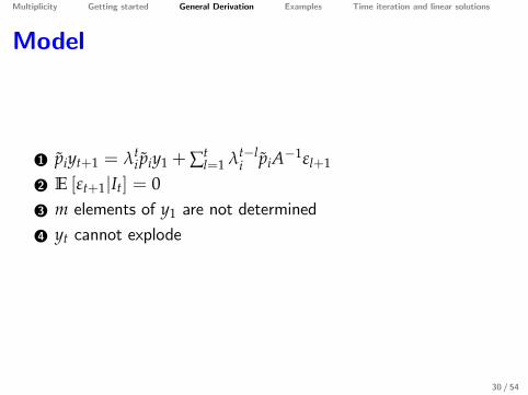
1 p̃iyt+1 = λti p̃iy1 +∑t
l=1 λt−li p̃iA−1εl+1
2 E [εt+1|It] = 03 m elements of y1 are not determined
4 yt cannot explode
30 / 54

Multiplicity Getting started General Derivation Examples Time iteration and linear solutions
Reasons for multiplicity
1 There are free elements in y1
2 The only constraint on eE,t+1 is that it is a prediction error.
• This leaves lots of freedom
31 / 54

Multiplicity Getting started General Derivation Examples Time iteration and linear solutions
Eigen values and multiplicity
• Suppose that |λ1| > 1• To avoid explosive behavior it must be the case that
1 p̃1y1 = 0 and
2 p̃1A−1εl = 0 ∀l
32 / 54

Multiplicity Getting started General Derivation Examples Time iteration and linear solutions
How to think about #1?
p̃1y1 = 0
• Simply an additional equation to pin down some of the freeelements
• Much better: This is the policy rule in the first period
33 / 54

Multiplicity Getting started General Derivation Examples Time iteration and linear solutions
How to think about #1?
p̃1y1 = 0
Neoclassical growth model:
• y1 = [k1, k0, z1]T
• |λ1| > 1, |λ2| < 1, λ3 = ρ < 1• p̃1y1 pins down k1 as a function of k0 and z1
• this is the policy function in the first period
34 / 54

Multiplicity Getting started General Derivation Examples Time iteration and linear solutions
How to think about #2?
p̃1A−1εl = 0 ∀l
• This pins down eE,t as a function of εz,t
• That is, the prediction error must be a function of thestructural shock, εz,t, and cannot be a function of other shocks,
• i.e., there are no sunspots
35 / 54

Multiplicity Getting started General Derivation Examples Time iteration and linear solutions
How to think about #2?
p̃1A−1εl = 0 ∀l
Neoclassical growth model:
• p̃1A−1εt says that the prediction error eE,t of period t is a fixedfunction of the innovation in period t of the exogenous process,ez,t
36 / 54

Multiplicity Getting started General Derivation Examples Time iteration and linear solutions
How to think about #1 combined with #2?
p̃1yt = 0 ∀t
• Without sunspots• i.e. with p̃1A−1εt = 0 ∀t
• kt is pinned down by kt−1 and zt in every period.
37 / 54

Multiplicity Getting started General Derivation Examples Time iteration and linear solutions
Blanchard-Kahn conditions
• Uniqueness: For every free element in y1, you need one λi > 1• Multiplicity: Not enough eigenvalues larger than one• No stable solution: Too many eigenvalues larger than one
38 / 54

Multiplicity Getting started General Derivation Examples Time iteration and linear solutions
How come this is so simple?• In practice, it is easy to get
Ayt+1 + Byt = εt+1
• How about the next step?
yt+1 = −A−1Byt +A−1εt+1
• Bad news: A is often not invertible• Good news: Same set of results can be derived
• Schur decomposition (See Klein 2000 and Soderlind 1999)39 / 54

Multiplicity Getting started General Derivation Examples Time iteration and linear solutions
How to check in Dynare
Use the following command after the model & initial conditions part
check;
40 / 54

Multiplicity Getting started General Derivation Examples Time iteration and linear solutions
Example - x predetermined - 1st order
xt−1 = φxt +Et [zt+1]
zt = 0.9zt−1 + εt
• |φ| > 1 : Unique stable fixed point• |φ| < 1 : No stable solutions; too many eigenvalues > 1
41 / 54

Multiplicity Getting started General Derivation Examples Time iteration and linear solutions
Example - x predetermined - 1st order
Corresponding state space system:[φ 10 1
] [xt
zt+1
]+
[−1 00 0.9
] [xt−1
zt
]=
[0
εt+1
]Λ =
[1/φ 0
0 0.9
]
• No sunspots, since Et [zt+1] is the only expectation.• No multiplicity because of free initial conditions either onestarting value for x given.
• So we just need stability =⇒ |φ| > 1
42 / 54

Multiplicity Getting started General Derivation Examples Time iteration and linear solutions
Example - x predetermined - 2nd order
φ2xt−1 = Et [φ1xt + xt+1 + zt+1]
zt = 0.9zt−1 + εt
• φ1 = −2.25, φ2 = −0.5 : Unique stable fixed point(1+ φ1L− φ2L2)xt = (1− 2L)(1− 1
4L)xt
• φ1 = −3.5, φ2 = −3 : No stable solution; too manyeigenvalues > 1(1+ φ1L− φ2L2)xt = (1− 2L)(1− 1.5L)xt
• φ1 = −1, φ2 = −0.25 : Multiple stable solutions; too feweigenvalues > 1(1+ φ1L− φ2L2)xt = (1− 0.5L)(1− 0.5L)xt
43 / 54

Multiplicity Getting started General Derivation Examples Time iteration and linear solutions
Example - x predetermined - 2nd order
Corresponding state space system: 1 φ1 10 1 00 0 1
xt+1xt
zt+1
+ 0 −φ2 0−1 0 00 0 −0.9
xtxt−1
zt
= eE,t+1
0εt
Λ =
2 0 00 0.9 00 0 0.25
• The Λ matrix is for the first numerical example (φ1 = −2.25,
φ2 = −0.5)
44 / 54

Multiplicity Getting started General Derivation Examples Time iteration and linear solutions
Example - x not predetermined - 1st order
xt = Et [φxt+1 + zt+1]
zt = 0.9zt−1 + εt
• |φ| < 1 : Unique stable fixed point• |φ| > 1 : Multiple stable solutions; too few eigenvalues > 1
45 / 54

Multiplicity Getting started General Derivation Examples Time iteration and linear solutions
Example - x not predetermined - 1st order
Corresponding state space system:[φ 10 1
] [xt+1zt+1
]+
[−1 00 0.9
] [xtzt
]=
[eE,t+1εt+1
]Λ =
[φ 00 0.9
]
• No sunspots, since Et [zt+1] is the only expectation.• No multiplicity because of free initial conditions either onestarting value for x given.
• So we just need stability =⇒ |φ| > 1
46 / 54
Multiplicity Getting started General Derivation Examples Time iteration and linear solutions
Solutions to linear systems
1 The analysis outlined above(requires A to be invertible)
2 Generalized version of analysis above(see Klein 2000)
3 Apply time iteration to linearized system(I learned this from Pontus Rendahl)
47 / 54

Multiplicity Getting started General Derivation Examples Time iteration and linear solutions
Solutions to linear systems
Model:Γ2kt+1 + Γ1kt + Γ0kt−1 = 0
or [Γ2 00 1
] [kt+1
kt
]+
[Γ1 Γ0−1 0
] [kt
kt−1
]= 0
48 / 54

Multiplicity Getting started General Derivation Examples Time iteration and linear solutions
Standard approaches
1 The method outlined above=⇒ a unique solution of the form
kt = akt−1
if BK conditions are satisfied
2 Impose that the solution is of the form
kt = akt−1
and solve for a from
Γ2a2kt−1 + Γ1akt−1 + Γ0kt−1 = 0 ∀kt−1
49 / 54

Multiplicity Getting started General Derivation Examples Time iteration and linear solutions
Time iteration
• Impose that the solution is of the form
kt = akt−1
• Use time iteration scheme, starting with a[1]
• Recall that time iteration means using the guess for tomorrowsbehavior and then solve for todays behavior
(This simple procedure was pointed out to me by Pontus Rendahl)
50 / 54

Multiplicity Getting started General Derivation Examples Time iteration and linear solutions
Time iteration
• Follow the following iteration scheme, starting with a[1]• Use a[i] to describe next period’s behavior. That is,
Γ2a[i]kt + Γ1kt + Γ0kt−1 = 0
(note the difference with last approach on previous slide)
• Obtain a[i+1] from
(Γ2a[i] + Γ1)kt + Γ0kt−1 = 0
kt = −(
Γ2a[i] + Γ1
)−1Γ0kt−1
a[i+1] = −(
Γ2a[i] + Γ1
)−1Γ0
51 / 54
Multiplicity Getting started General Derivation Examples Time iteration and linear solutions
Advantages of time iteration
• It is simple even if the "A matrix" is not invertible.(the inversion required by time iteration seems less problematicin practice)
• Since time iteration is linked to value function iteration, it hasnice convergence properties
52 / 54

Multiplicity Getting started General Derivation Examples Time iteration and linear solutions
Example
kt+1 − 2kt + 0.75kt−1 = 0
• The two solutions are
kt = 0.5kt−1 & kt = 1.5kt−1
• Time iteration on kt = a[i]kt−1 converges to stable solution forall initial values of a[i] except 1.5.
53 / 54
Multiplicity Getting started General Derivation Examples Time iteration and linear solutions
References and Acknowledgements• Larry Christiano taught me (a long time ago) this simple way of deriving the BK
conditions and I think that I did not even change the notation.
• Blanchard, Olivier and Charles M. Kahn, 1980,The Solution of Linear Difference Models
under Rational Expectations, Econometrica, 1305-1313.
• Den Haan, Wouter J., 2007, Shocks and the Unavoidable Road to Higher Taxes and
Higher Unemployment, Review of Economic Dynamics, 348-366.
• simple model in which the size of the shocks has long-term consequences
• Farmer, Roger, 1993, The Macroeconomics of Self-Fulfilling Prophecies, The MIT Press.
• textbook by the pioneer
• Klein, Paul, 2000, Using the Generalized Schur form to Solve a Multivariate Linear
Rational Expectations Model, Journal of Economic Dynamics and Control, 1405-1423.
• in case you want to do the analysis without the simplifying assumption that A is
invertible
• Soderlind, Paul, 1999, Solution and estimation of RE macromodels with optimal policy,
European Economic Review, 813-823
• also doesn’t assume that A is invertible; possibly a more accessible paper54 / 54