Stability of a circular tunnel in cohesive-frictional soil ... of a circular tunnel in cohesive-frictional ... Six types of rigid-block mechanisms were constructed, as shown ... frictional

Computers and Geotechnics 38 (2011) 504–514

Contents lists available at ScienceDirect

Computers and Geotechnics

journal homepage: www.elsevier .com/ locate/compgeo

Stability of a circular tunnel in cohesive-frictional soil subjectedto surcharge loading

Kentaro Yamamoto a,⇑, Andrei V. Lyamin b, Daniel W. Wilson b, Scott W. Sloan b, Andrew J. Abbo b

a Department of Ocean Civil Engineering, Kagoshima University, Kagoshima 890-0065, Japanb Centre for Geotechnical and Materials Modelling, University of Newcastle, NSW 2308, Australia

a r t i c l e i n f o

Article history:Received 14 December 2010Received in revised form 22 February 2011Accepted 23 February 2011Available online 21 March 2011

Keywords:Shallow tunnelStabilityRigid-block mechanismLimit analysisFinite elements

0266-352X/$ - see front matter � 2011 Elsevier Ltd.doi:10.1016/j.compgeo.2011.02.014

⇑ Corresponding author. Tel.: +81 99 285 8475.E-mail address: [email protected] (

a b s t r a c t

The stability of circular tunnels in cohesive-frictional soils subjected to surcharge loading has been inves-tigated theoretically and numerically assuming plane strain conditions. Despite the importance of thisproblem, previous research on the subject is very limited. At present, no generally accepted design oranalysis method is available to evaluate the stability of tunnels/openings in cohesive-frictional soils. Inthis study, continuous loading is applied to the ground surface, and both smooth and rough interface con-ditions are modelled. For a series of tunnel diameter-to-depth ratios and material properties, rigorouslower- and upper-bound solutions for the ultimate surcharge loading are obtained by applying finite ele-ment limit analysis techniques. For practical use, the results are presented in the form of dimensionlessstability charts with the actual tunnel stability numbers being closely bracketed from above and below.As an additional check on the solutions, upper-bound rigid-block mechanisms have been developed andthe predicted collapse loads from these are compared with those from finite element limit analysis.Finally, an expression that approximates the ultimate surcharge load has been devised which is conve-nient for use by practising engineers.

� 2011 Elsevier Ltd. All rights reserved.

1. Introduction mechanisms are developed and the solutions from these are com-

Accurately assessing the stability of circular tunnels, pipelinesand disused mine workings in cohesive-frictional soils is an impor-tant task due to the ubiquitous construction of buildings and tun-nels in urban areas. Since many tunnels and pipelines alreadyexist at deep levels, new tunnels and openings are now often beingconstructed at shallow depths. In these cases, it is important toknow how the stability of these tunnels/openings is affected by sur-charge loading. As no generally accepted design or analysis methodis available currently for this problem, the goal of this study is toequip design engineers with simple design tools to determine thestability of circular tunnels in cohesive-frictional soils subjectedto surcharge loading. Drained loading conditions are considered,and a continuous load is applied to the ground surface with bothsmooth and rough interface conditions. For a series of tunnel diam-eter-to-depth ratios and material properties, rigorous lower- andupper-bound solutions for the ultimate surcharge loading are foundby applying finite element limit analysis techniques [1,2]. Theresults are presented as dimensionless stability charts for use bypractising engineers, and the actual tunnel stability numbers clo-sely bracketed from above and below. As an additional check onthe accuracy of the results, a variety of upper-bound rigid-block

All rights reserved.

K. Yamamoto).

pared with those from finite element limit analysis.The stability of circular tunnels was studied extensively studied

at Cambridge in the 1970s; see, for example, the work reported byCairncross [3], Atkinson and Cairncross [4], Mair [5],

Seneviratne [6] and Davis et al. [7]. Later, theoretical solutionsfor circular tunnel problems under drained conditions were deter-mined by Muhlhaus [8] and Leca and Dormieux [9].

The application of finite element limit analysis to the undrainedstability of shallow tunnels was first considered by Sloan and Assadi[10], who investigated the case of a plane strain circular tunnel incohesive soil whose shear strength varied linearly with depth usinglinear programming techniques. Later, Lyamin and Sloan [11]considered the stability of a plane strain circular tunnel in a cohe-sive-frictional soil using a more efficient non-linear programmingtechnique. This method can accommodate large numbers of finiteelements, thus resulting in very accurate solutions. Recently,Yamamoto et al. [12] studied the stability of shallow circular andsquare tunnels in cohesive-frictional soils subjected to surchargeloading, which is developed further in the present paper.

2. Problem description

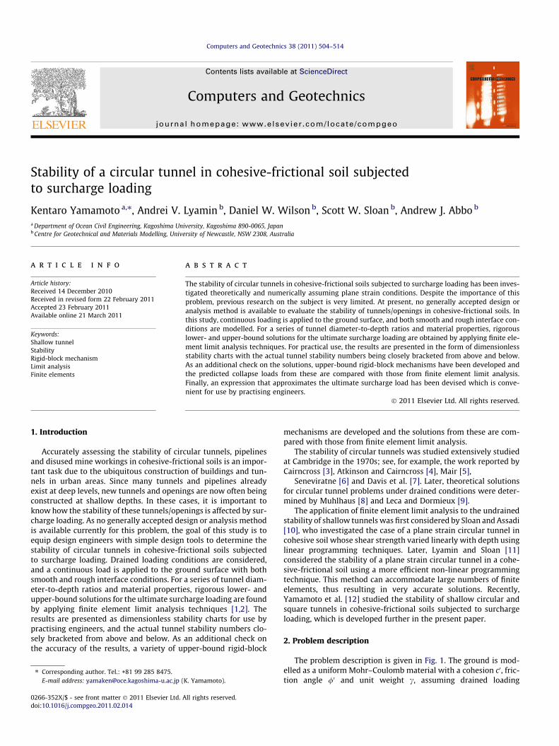
The problem description is given in Fig. 1. The ground is mod-elled as a uniform Mohr–Coulomb material with a cohesion c0, fric-tion angle /0 and unit weight c, assuming drained loading

http://dx.doi.org/10.1016/j.compgeo.2011.02.014

mailto:[email protected]

http://dx.doi.org/10.1016/j.compgeo.2011.02.014

http://www.sciencedirect.com/science/journal/0266352X

http://www.elsevier.com/locate/compgeo

Cohesion=c’ H

CL

D

sσ

Friction angle= 'φ

Unit weight=

Fig. 1. Plane strain circular tunnel in cohesive-frictional soil.

K. Yamamoto et al. / Computers and Geotechnics 38 (2011) 504–514 505

conditions. The circular tunnel is of diameter D and depth H, anddeformation takes place under plane strain. The stability of theshallow tunnel shown in Fig. 1 is described conveniently bythe dimensionless load parameter rs/c0, which is a function of /0,cD/c0 and H/D as shown in the following equation:

rs=c0 ¼ f ð/0; cD=c0;H=DÞ ð1Þ

Formulating the problem in this manner permits a compact set ofstability charts to be constructed, which are useful for designpurposes. The problem parameters considered in this paper areH/D = 1–5, /0 = 0–35� and cD/c0 = 0–3. The continuous (flexible)loading is applied to the ground surface with both smooth andrough interface conditions. To model the smooth interface condi-tion between the loading and the soil, the shear stress is fixedto zero (s = 0) along the ground surface in the lower-bound anal-yses, with no velocity constraints being imposed in the upper-bound analyses. For the rough case, the horizontal velocity is fixedto zero (u = 0) along the ground surface in the upper-bound anal-yses, with no stress constraints being imposed in the lower-boundanalyses.

3. Finite element limit analysis

Finite element limit analysis utilises the power of the lower-and upper-bound theorems of plasticity theory, coupled with finiteelements, to provide rigorous bounds on collapse loads from bothbelow and above. The underlying limit theorems assume a rigid-plastic soil with an associated flow rule. The use of a finite elementdiscretization of the soil, combined with mathematical optimisa-tion to maximise the lower bound and minimise the upper bound,makes it possible to handle problems with layered soils, complexgeometries and complicated loading conditions. The formulationsof the numerical limit analysis used in this paper originate fromthose given by Sloan [13,14] and Sloan and Kleeman [15], who em-ployed active-set linear programming and discontinuous stressand velocity fields to solve a variety of practical stability problems.Since then, numerical limit analysis has evolved significantly withthe advent of very fast non-linear optimisation solvers, and thetechniques used in this paper are those described by Lyamin andSloan [1] and Krabbenhøft et al. [2].

Briefly, these formulations use linear stress (lower bound) andlinear velocity (upper bound) triangular finite elements to

discretize the soil mass. In contrast to conventional displacementfinite element analysis, each node in the limit analysis mesh is un-ique to a particular element so that statically admissible stress andkinematically admissible velocity discontinuities are permitted in,respectively, the lower-bound and upper-bound formulations. Theobjective of the lower-bound analysis is to maximise the load mul-tiplier subject to the element equilibrium, stress boundary condi-tions and yield constraints. For the upper-bound analysis, theinternal power dissipation minus the rate of work done by the pre-scribed external forces is minimised with respect to the velocityboundary conditions, compatibility and flow rule constraints. Bothformulations result in convex mathematical programs, which(after considering the dual to the upper-bound optimisation prob-lem) can be cast in the following form:

Maximise k

subject to Ar ¼ p0 þ kpfiðrÞ 6 0; i ¼ f1; . . . ;Ng

ð2Þ

where k is a load multiplier, r is a vector of stress variables, A is amatrix of equality constraint coefficients, p0 and p are vectors ofprescribed and optimizable forces, fi is the yield function for thestress set i, and N is the number of stress nodes.

The solutions to problem (2) can be found very efficiently bysolving the system of non-linear equations that define its Kuhn-Tucker optimality conditions. The interior point procedure usedis based on efficient conic programming implementation, re-quires usually 30–50 iterations, regardless of the problem size,and is many times faster than previously employed linear pro-gramming schemes. The solutions of the lower- and upper-bound computations bracket the actual collapse load from belowand above and, thus, give a clear indication of the accuracy ofthe results.

Fig. 2a and b shows the lower-bound and upper-bound half-meshes for H/D = 3 with rough interfaces. The meshes are symmet-ric, and similar meshes are used for the lower- and upper-boundanalyses. The lower-bound mesh has 20,000 triangular elementsand 29,850 stress discontinuities, while the upper-bound meshhas 28,800 triangular elements and 43,020 velocity discontinuities.In the lower-bound analysis, extension elements are includedalong the soil domain boundaries to represent a semi-infinitematerial. This feature is necessary to guarantee that the lowerbounds are fully rigorous, and is a convenient means of extendingthe stress field throughout a semi-infinite domain in a mannerwhich satisfies equilibrium, the stress boundary conditions andthe yield criterion. The size of the soil domain for each of the tun-nel geometries considered is chosen such that the plasticity zone atfailure lies well inside the domain. Careful mesh refinement is re-quired to obtain accurate solutions, with the mesh density beinghigh around the tunnel face with a smooth transition to larger ele-ments near the boundary of the mesh.

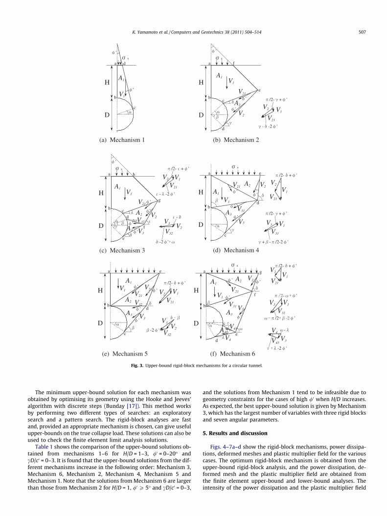
4. Upper-bound rigid-block analysis

Semi-analytical rigid-block methods were used to find upper-bound solutions for the cases considered. These provided an addi-tional check on the limit analysis results. Six types of rigid-blockmechanisms were constructed, as shown in Fig. 3. In this Figure,Ai is the area of the rigid block i; Vi is the kinematically admissiblevelocity of block i; Vij is the velocity jump along the discontinuitybetween blocks i and j; lij is the distance between points i and j;(a, b, c, d, e, k, x) are angles that determine the geometry of therigid-block mechanism; and /0 is the dilatancy angle. The compat-ible velocity diagrams using Vi and Vij are given at the right side ofthe block mechanisms. All velocities can be obtained using thegeometry of these diagrams. With an associated flow rule we

(a) Lower-bound mesh (b) Upper-bound mesh

H

H

D=

0=

0n=

=0

sσ

=0

u=v=0

u=0

u=0

D

H

H

sσ

u=0

u=0

u

v

Fig. 2. Typical finite element meshes for a circular tunnel (H/D = 3, rough interface).

506 K. Yamamoto et al. / Computers and Geotechnics 38 (2011) 504–514

assume the dilatancy angle is equal to the friction angle. Althoughit is well known that the use of an associated flow rule predictsexcessive dilation during shear failure of frictional soils, it is unli-kely this feature will have a major impact on the predicted limitloads for cases with low to moderate friction angles. Generallyspeaking, any inaccuracy caused by an associated flow rule willbe most pronounced for soils with very high friction angles and/or problems that are subject to high degrees of kinematic con-straint (which is not the case for the tunnel considered here).Mechanism 1 is a simple roof collapse mechanism which is

Mechanism 1

rs 6c0lcd cos /0 � A1c

lad

Mechanism 2

rs 6cð0V1lef cos /0 þ V2lde cos /0 þ V21lce cos /0Þ � cðA1V1 þ A2V2 sinðc�

V1laf

Mechanism 3

rs 6c0ðV1lgh cos /0 þ V2lfg cos /0 þ V21lcg cos /0 þ V3lef cos /0 þ V32ldf cos

V1lah

Mechanism 4

rs 6c0ðV2lde cos /0 þ V21lad cos /0 þ V31lbd cos /0 þ V3lcd cos /0Þ � cðA1V1

V2lae sinðd� /0Þ

Mechanism 5

rs 6c0ðV2lde cos /0 þ V21lbe cos /0 þ V32lbd cos /0 þ V3lcd cos /0Þ � cðA1V1

V1lae

Mechanism 6

rs 6c0ðV2lfg cos /0 þ V21laf cos /0 þ V31lbf cos /0 þ V3lef cos /0 þ V43lce cos

V2lag sinðd� /0Þ

� �cðA1V1 þ A2V2 sinðd� /0Þ þ A3V3 sinðx� /0Þ þ A4V4 sinðk� /

V2lag sinðd� /0Þ

suitable for shallow tunnels, while the mechanisms 2–6 are morecomplex examples of both roof and side collapse mechanisms.The total number of angular parameters for mechanisms 1–6 are1, 4, 7, 4, 3 and 7, respectively. The soil mass was assumed to begoverned by the Mohr–Coulomb failure criterion and an associatedflow rule, with the geometry of the blocks being allowed to varywhile being constrained such that their areas and boundary seg-ment lengths remain non-negative. The details of rigid-block anal-ysis can be found in Chen [16]. The upper-bound solutions derivedfrom mechanisms 1–6 are given as follows:

ð3Þ

/0ÞÞ ð4Þ

/0Þ � cðA1V1 þ A2V2 sinðe� /0Þ þ A3V3 sinðd� /0ÞÞ ð5Þ

þ A2V2 sinðd� /0Þ þ A3V3 sinðc� /0ÞÞ ð6Þ

þ A2V2 sinðd� /0Þ þ A3V3 sinðb� /0ÞÞ ð7Þ

/0 þ V4lde cos /0Þ

0ÞÞ ð8Þ

(a) Mechanism 1 (b) Mechanism 2

(c) Mechanism 3 (d) Mechanism 4

'

V1

s

A1H

D

'

a

b

c

d

'

V1

V21

V2V32

V3

s

A1

A2

D

H

a

b cd

e

f

g

h

'

'

'

'A3

'

V1

V21

V2

s

A1

A2

H

D'

'

a

bc

d

e

f

V1V2

V21

/2- + '

- -2 '

V1V2

V21

/2- + '

- -2 '

V2

V3

V32

-2 '

-

V1

V21 V2

V31

V3

s

A1

A2

H

D

''

'

'

a

b

c

d

e

A3

V1

V2

V21

/2- + '

V1V3

V31

/2- + '

+ - /2-2 '

(e) Mechanism 5 (f) Mechanism 6

V2

V3

V32-2 ' '

V1

V21

V2

V43

V4

A1A2

A4

D

H

a

b

c

de

f

g

'

'

' '

A3

V3V31

s

V1V3

V31

- '

/2 - '

/2- + '

V1

V2

V21

V3

V4

V43

-2 '

-

V1V21

V2

V32

V3

A1

A2

A3

H

D

''

'

'

a

b

c

d

e

V1V2

V21

/2- + '

Fig. 3. Upper-bound rigid-block mechanisms for a circular tunnel.


The minimum upper-bound solution for each mechanism wasobtained by optimising its geometry using the Hooke and Jeeves’algorithm with discrete steps (Bunday [17]). This method worksby performing two different types of searches: an exploratorysearch and a pattern search. The rigid-block analyses are fastand, provided an appropriate mechanism is chosen, can give usefulupper-bounds on the true collapse load. These solutions can also beused to check the finite element limit analysis solutions.

Table 1 shows the comparison of the upper-bound solutions ob-tained from mechanisms 1–6 for H/D = 1–3, /0 = 0–20� andcD/c0 = 0–3. It is found that the upper-bound solutions from the dif-ferent mechanisms increase in the following order: Mechanism 3,Mechanism 6, Mechanism 2, Mechanism 4, Mechanism 5 andMechanism 1. Note that the solutions from Mechanism 6 are largerthan those from Mechanism 2 for H/D = 1, /0 P 5� and cD/c0 = 0–3,

and the solutions from Mechanism 1 tend to be infeasible due togeometry constraints for the cases of high /0 when H/D increases.As expected, the best upper-bound solution is given by Mechanism3, which has the largest number of variables with three rigid blocksand seven angular parameters.

5. Results and discussion

Figs. 4–7a–d show the rigid-block mechanisms, power dissipa-tions, deformed meshes and plastic multiplier field for the variouscases. The optimum rigid-block mechanism is obtained from theupper-bound rigid-block analysis, and the power dissipation, de-formed mesh and the plastic multiplier field are obtained fromthe finite element upper-bound and lower-bound analyses. Theintensity of the power dissipation and the plastic multiplier field

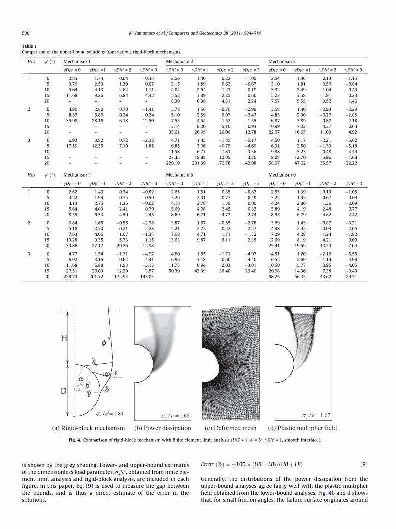
Table 1Comparison of the upper-bound solutions from various rigid-block mechanisms.

H/D /0 (�) Mechanism 1 Mechanism 2 Mechanism 3

cD/c0 = 0 cD/c0 = l cD/c0 = 2 cD/c0 = 3 cD/c0 = 0 cD/c0 = l cD/c0 = 2 cD/c0 = 3 cD/c0 = 0 cD/c0 = l cD/c0 = 2 cD/c0 = 3

1 0 2.83 1.74 0.64 �0.45 2.56 1.40 0.22 �1.00 2.54 1.36 0.13 �1.155 3.76 2.53 1.30 0.07 3.15 1.89 0.62 �0.67 3.10 1.81 0.50 �0.84

10 5.64 4.13 2.62 1.11 4.04 2.64 1.23 �0.19 3.92 2.49 1.04 �0.4315 11.68 9.26 6.84 4.42 5.52 3.89 2.25 0.60 5.23 3.58 1.91 0.2320 – – – – 8.39 6.36 4.31 2.24 7.57 5.55 3.52 1.46

2 0 4.90 2.80 0.70 �1.41 3.78 1.56 �0.70 �2.99 3.68 1.40 �0.93 �3.295 8.57 5.80 0.24 0.24 5.10 2.59 0.07 �2.47 4.85 2.30 �0.27 �2.85

10 35.98 28.16 6.18 12.50 7.53 4.54 1.52 �1.55 6.87 3.89 0.87 �2.1815 – – – – 13.14 9.20 5.16 0.93 10.99 7.23 3.37 �0.6420 – – – – 33.61 26.95 20.06 12.78 22.07 16.65 11.00 4.92

3 0 6.93 3.82 0.72 �2.38 4.71 1.45 �1.85 �5.17 4.50 1.17 �2.21 �5.625 17.59 12.35 7.10 1.85 6.85 3.06 �0.75 �4.60 6.31 2.50 �1.33 �5.18

10 – – – – 11.58 6.77 1.83 �3.36 9.88 5.23 0.48 �4.4915 – – – – 27.35 19.88 12.05 3.36 19.08 12.70 5.96 �1.6820 – – – – 229.19 201.39 172.78 142.98 58.97 47.62 35.57 22.22

H/D /0 (�) Mechanism 4 Mechanism 5 Mechanism 6

cD/c0 = 0 cD/c0 = l cD/c0 = 2 cD/c0 = 3 cD/c0 = 0 cD/c0 = l cD/c0 = 2 cD/c0 = 3 cD/c0 = 0 cD/c0 = l cD/c0 = 2 cD/c0 = 3

1 0 2.62 1.49 0.34 �0.82 2.65 1.51 0.35 �0.82 2.55 1.39 0.19 �1.055 3.22 1.99 0.75 �0.50 3.26 2.01 0.77 �0.49 3.22 1.95 0.67 �0.64

10 4.13 2.75 1.36 �0.02 4.18 2.78 1.39 0.00 4.24 2.80 1.36 �0.0915 5.64 4.03 2.41 0.79 5.69 4.08 2.45 0.82 5.89 4.19 2.48 0.7720 8.55 6.53 4.50 2.45 8.69 6.71 4.72 2.74 8.95 6.79 4.62 2.42

2 0 3.84 1.65 �0.56 �2.78 3.87 1.67 �0.55 �2.78 3.69 1.43 �0.87 �3.215 5.18 2.70 0.21 �2.28 5.21 2.72 0.22 �2.27 4.98 2.45 �0.09 �2.65

10 7.63 4.66 1.67 �1.35 7.68 4.71 1.71 �1.32 7.29 4.28 1.24 �1.8215 13.28 9.35 5.33 1.15 13.63 9.87 6.11 2.35 12.09 8.19 4.21 0.0920 33.86 27.17 20.26 12.98 – – – – 25.41 19.59 13.53 7.04

3 0 4.77 1.54 �1.71 �4.97 4.80 1.55 �1.71 �4.97 4.51 1.20 �2.16 �5.555 6.92 3.16 �0.62 �4.41 6.96 3.18 �0.60 �4.40 6.52 2.69 �1.14 �4.99

10 11.68 6.88 1.98 �3.13 11.73 6.94 2.03 �3.01 10.50 5.77 0.95 �4.0515 27.51 20.03 12.20 3.57 50.39 43.39 36.40 29.40 20.98 14.36 7.38 �0.4320 229.73 201.72 172.93 143.03 – – – – 68.25 56.35 43.62 29.51

81.1'/ =csσ

(a) Rigid-block mechanism (b) Power dissipation (c) Deformed mesh (d) Plastic multiplier field

68.1'/ =csσ 67.1'/ =csσ

Fig. 4. Comparison of rigid-block mechanism with finite element limit analysis (H/D = 1, /0 = 5�, cD/c0 = 1, smooth interface).


is shown by the grey shading. Lower- and upper-bound estimatesof the dimensionless load parameter, rs/c0, obtained from finite ele-ment limit analysis and rigid-block analysis, are included in eachfigure. In this paper, Eq. (9) is used to measure the gap betweenthe bounds, and is thus a direct estimate of the error in thesolutions.

Error ð%Þ ¼ �100� ðUB� LBÞ=ðUBþ LBÞ ð9Þ

Generally, the distributions of the power dissipation from theupper-bound analyses agree fairly well with the plastic multiplierfield obtained from the lower-bound analyses. Fig. 4b and d showsthat, for small friction angles, the failure surface originates around

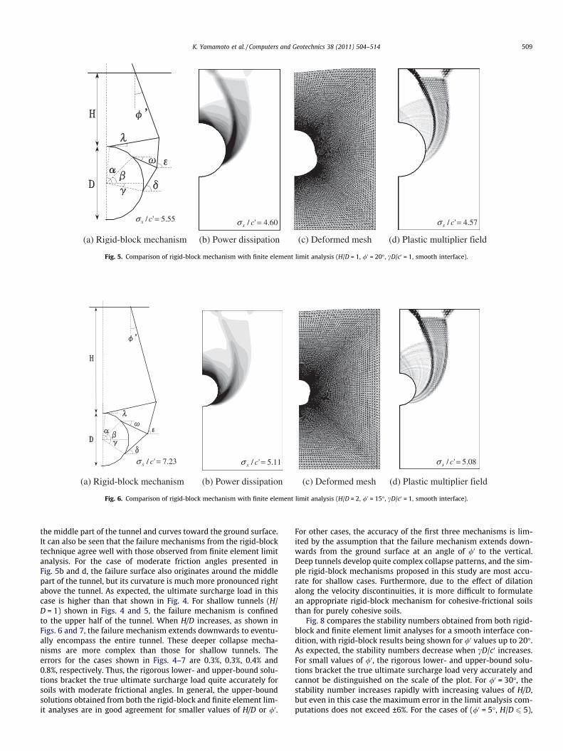
55.5'/ =csσ 60.4'/ =csσ 57.4'/ =csσ



23.7'/ =csσ

(a) Rigid-block mechanism (c) Deformed mesh (d) Plastic multiplier field

11.5'/ =csσ 08.5'/ =csσ

(b) Power dissipation



the middle part of the tunnel and curves toward the ground surface.It can also be seen that the failure mechanisms from the rigid-blocktechnique agree well with those observed from finite element limitanalysis. For the case of moderate friction angles presented inFig. 5b and d, the failure surface also originates around the middlepart of the tunnel, but its curvature is much more pronounced rightabove the tunnel. As expected, the ultimate surcharge load in thiscase is higher than that shown in Fig. 4. For shallow tunnels (H/D = 1) shown in Figs. 4 and 5, the failure mechanism is confinedto the upper half of the tunnel. When H/D increases, as shown inFigs. 6 and 7, the failure mechanism extends downwards to eventu-ally encompass the entire tunnel. These deeper collapse mecha-nisms are more complex than those for shallow tunnels. Theerrors for the cases shown in Figs. 4–7 are 0.3%, 0.3%, 0.4% and0.8%, respectively. Thus, the rigorous lower- and upper-bound solu-tions bracket the true ultimate surcharge load quite accurately forsoils with moderate frictional angles. In general, the upper-boundsolutions obtained from both the rigid-block and finite element lim-it analyses are in good agreement for smaller values of H/D or /0.

For other cases, the accuracy of the first three mechanisms is lim-ited by the assumption that the failure mechanism extends down-wards from the ground surface at an angle of /0 to the vertical.Deep tunnels develop quite complex collapse patterns, and the sim-ple rigid-block mechanisms proposed in this study are most accu-rate for shallow cases. Furthermore, due to the effect of dilationalong the velocity discontinuities, it is more difficult to formulatean appropriate rigid-block mechanism for cohesive-frictional soilsthan for purely cohesive soils.

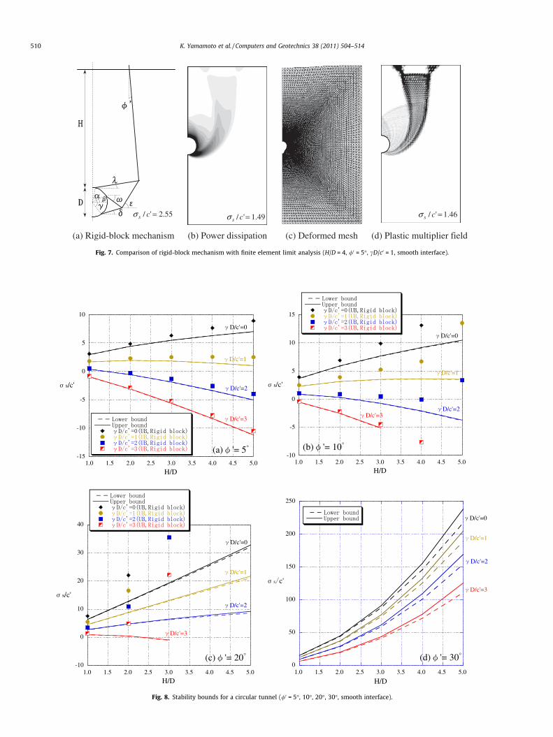
Fig. 8 compares the stability numbers obtained from both rigid-block and finite element limit analyses for a smooth interface con-dition, with rigid-block results being shown for /0 values up to 20�.As expected, the stability numbers decrease when cD/c0 increases.For small values of /0, the rigorous lower- and upper-bound solu-tions bracket the true ultimate surcharge load very accurately andcannot be distinguished on the scale of the plot. For /0 = 30�, thestability number increases rapidly with increasing values of H/D,but even in this case the maximum error in the limit analysis com-putations does not exceed ±6%. For the cases of (/0 = 5�, H/D 6 5),


55.2'/ =csσ 49.1'/ =csσ 46.1'/ =csσ


-15

-10

-5

0

5

10

1.0 1.5 2.0 2.5 3.0 3.5 4.0 4.5 5.0

H/D

s/c'

(a) '= 5

D/c'=0

D/c'=1

D/c'=2

D/c'=3

-10

-5

0

5

10

15

1.0 1.5 2.0 2.5 3.0 3.5 4.0 4.5 5.0

s/c'

H/D

(b) '= 10

D/c'=0

D/c'=1

D/c'=2D/c'=3

-10

0

10

20

30

40

1.0 1.5 2.0 2.5 3.0 3.5 4.0 4.5 5.0

s/c'

H/D

(c) '= 20

D/c'=0

D/c'=1

D/c'=2

D/c'=3

0

50

100

150

200

250

1.0 1.5 2.0 2.5 3.0 3.5 4.0 4.5 5.0

s c'

H/D

(d) '= 30

D/c'=0

D/c'=1

D/c'=2

D/c'=3

Fig. 8. Stability bounds for a circular tunnel (/0 = 5�, 10�, 20�, 30�, smooth interface).


-15

-10

-5

0

5

10

1.0 1.5 2.0 2.5 3.0 3.5 4.0 4.5 5.0

H/D

s/c'

(a) '= 5

D/c'=0

D/c'=1

D/c'=2

D/c'=3

-10

-5

0

5

10

15

1.0 1.5 2.0 2.5 3.0 3.5 4.0 4.5 5.0

H/D

s/c'

(b) '= 10

D/c'=0

D/c'=1

D/c'=2

D/c'=3

-5

0

5

10

15

20

25

30

35

1.0 1.5 2.0 2.5 3.0 3.5 4.0 4.5 5.0

H/D

s/c'

(c) '= 20

D/c'=0

D/c'=1

D/c'=2

D/c'=3

0

50

100

150

200

250

300

1.0 1.5 2.0 2.5 3.0 3.5 4.0 4.5 5.0

s c'

H/D

(d) '= 30

D/c'=0

D/c'=1

D/c'=2

D/c'=3

Fig. 9. Stability bounds for a circular tunnel (/0 = 5�, 10�, 20�, 30�, rough interface).

Table 2Coefficients of empirical equation.

Parameters Smooth interface Rough interface

a 1.492521 1.558360b 0.070218 0.068660c 1.040522 1.059821d 0.472325 0.466462e 0.015413 0.016675f 1.317933 1.295656g �0.495490 �0.479079h 0.010923 0.010225k 0.464155 0.478401m �0.012827 �0.013290


(/0 = 10�, H/D 6 3) and (/0 = 20�, H/D 6 1), the upper-bound solu-tions from the rigid-block method agree well with those obtainedfrom finite element limit analysis. However, for cases with high val-ues of H/D or /0, the accuracy of the solutions from all the rigid-block mechanisms becomes poor. In some cases where cD/c0 = 3and H/D P 4, as shown in Fig. 8b and c, feasible solutions fromthe rigid-block and finite element limit analyses could not be ob-tained because the tunnel undergoes local roof collapse due tothe effect of soil self-weight. Note that the sign convention for thestability charts is that a positive value of the stability number im-plies that the ground can support a compressive normal stress,

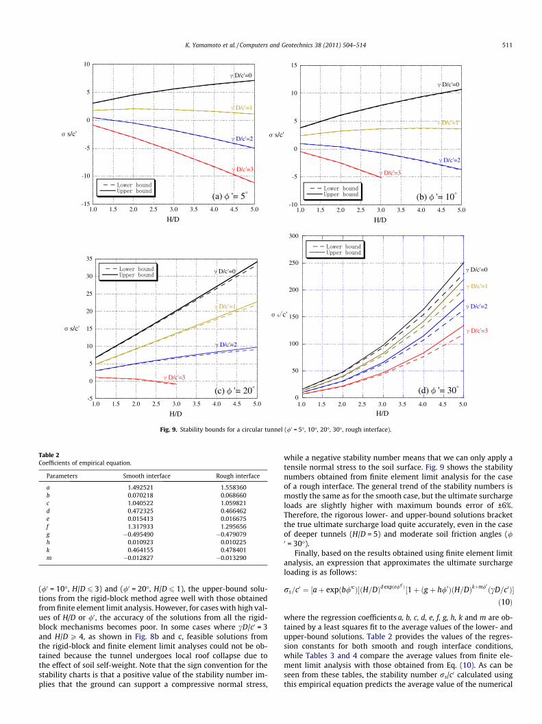
while a negative stability number means that we can only apply atensile normal stress to the soil surface. Fig. 9 shows the stabilitynumbers obtained from finite element limit analysis for the caseof a rough interface. The general trend of the stability numbers ismostly the same as for the smooth case, but the ultimate surchargeloads are slightly higher with maximum bounds error of ±6%.Therefore, the rigorous lower- and upper-bound solutions bracketthe true ultimate surcharge load quite accurately, even in the caseof deeper tunnels (H/D = 5) and moderate soil friction angles (/0 = 30�).

Finally, based on the results obtained using finite element limitanalysis, an expression that approximates the ultimate surchargeloading is as follows:

rs=c0 ¼ ½aþ expðb/0cÞ�ðH=DÞd expðe/0f Þ½1þ ðg þ h/0ÞðH=DÞkþm/0 ðcD=c0Þ�ð10Þ

where the regression coefficients a, b, c, d, e, f, g, h, k and m are ob-tained by a least squares fit to the average values of the lower- andupper-bound solutions. Table 2 provides the values of the regres-sion constants for both smooth and rough interface conditions,while Tables 3 and 4 compare the average values from finite ele-ment limit analysis with those obtained from Eq. (10). As can beseen from these tables, the stability number rs/c0 calculated usingthis empirical equation predicts the average value of the numerical

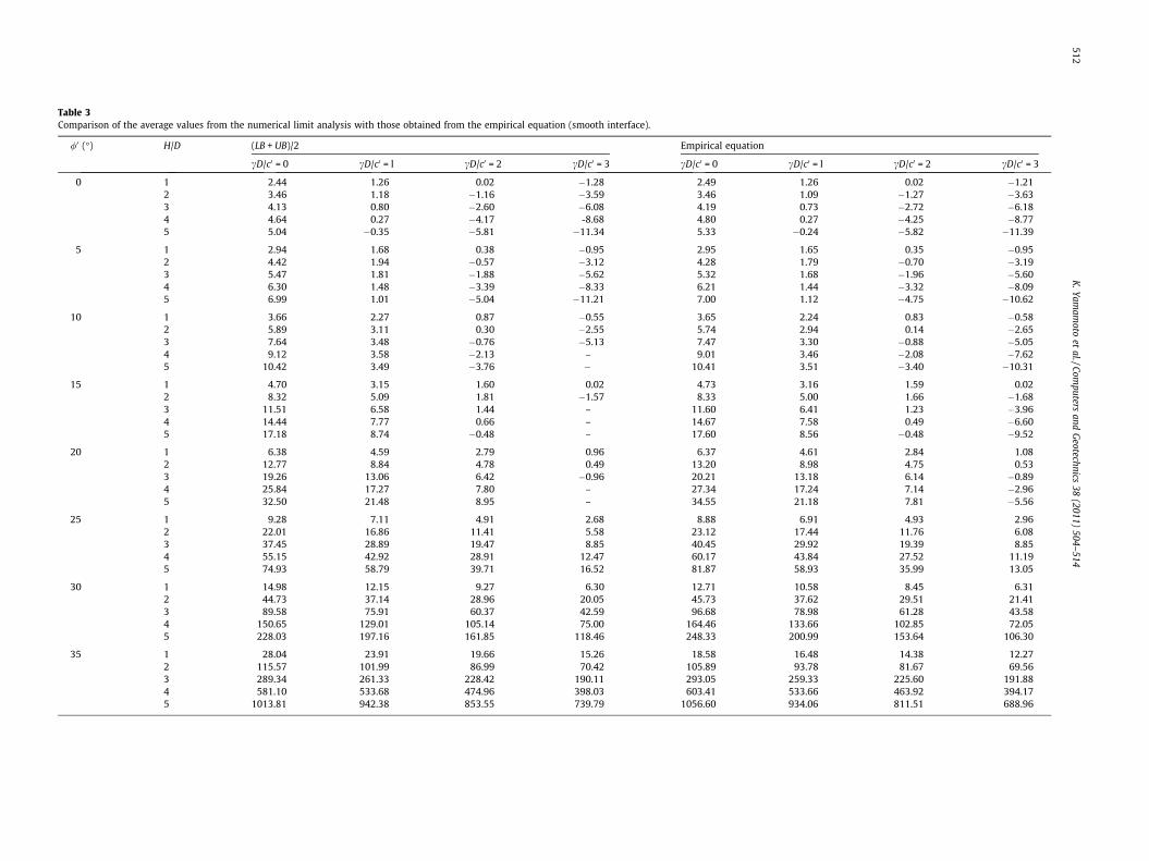
Table 3Comparison of the average values from the numerical limit analysis with those obtained from the empirical equation (smooth interface).

/0 (�) H/D (LB + UB)/2 Empirical equation

cD/c0 = 0 cD/c0 = l cD/c0 = 2 cD/c0 = 3 cD/c0 = 0 cD/c0 = l cD/c0 = 2 cD/c0 = 3

0 1 2.44 1.26 0.02 �1.28 2.49 1.26 0.02 �1.212 3.46 1.18 �1.16 �3.59 3.46 1.09 �1.27 �3.633 4.13 0.80 �2.60 �6.08 4.19 0.73 �2.72 �6.184 4.64 0.27 �4.17 -8.68 4.80 0.27 �4.25 �8.775 5.04 �0.35 �5.81 �11.34 5.33 �0.24 �5.82 �11.39

5 1 2.94 1.68 0.38 �0.95 2.95 1.65 0.35 �0.952 4.42 1.94 �0.57 �3.12 4.28 1.79 �0.70 �3.193 5.47 1.81 �1.88 �5.62 5.32 1.68 �1.96 �5.604 6.30 1.48 �3.39 �8.33 6.21 1.44 �3.32 �8.095 6.99 1.01 �5.04 �11.21 7.00 1.12 �4.75 �10.62

10 1 3.66 2.27 0.87 �0.55 3.65 2.24 0.83 �0.582 5.89 3.11 0.30 �2.55 5.74 2.94 0.14 �2.653 7.64 3.48 �0.76 �5.13 7.47 3.30 �0.88 �5.054 9.12 3.58 �2.13 – 9.01 3.46 �2.08 �7.625 10.42 3.49 �3.76 � 10.41 3.51 �3.40 �10.31

15 1 4.70 3.15 1.60 0.02 4.73 3.16 1.59 0.022 8.32 5.09 1.81 �1.57 8.33 5.00 1.66 �1.683 11.51 6.58 1.44 – 11.60 6.41 1.23 �3.964 14.44 7.77 0.66 – 14.67 7.58 0.49 �6.605 17.18 8.74 �0.48 – 17.60 8.56 �0.48 �9.52

20 1 6.38 4.59 2.79 0.96 6.37 4.61 2.84 1.082 12.77 8.84 4.78 0.49 13.20 8.98 4.75 0.533 19.26 13.06 6.42 �0.96 20.21 13.18 6.14 �0.894 25.84 17.27 7.80 – 27.34 17.24 7.14 �2.965 32.50 21.48 8.95 – 34.55 21.18 7.81 �5.56

25 1 9.28 7.11 4.91 2.68 8.88 6.91 4.93 2.962 22.01 16.86 11.41 5.58 23.12 17.44 11.76 6.083 37.45 28.89 19.47 8.85 40.45 29.92 19.39 8.854 55.15 42.92 28.91 12.47 60.17 43.84 27.52 11.195 74.93 58.79 39.71 16.52 81.87 58.93 35.99 13.05

30 1 14.98 12.15 9.27 6.30 12.71 10.58 8.45 6.312 44.73 37.14 28.96 20.05 45.73 37.62 29.51 21.413 89.58 75.91 60.37 42.59 96.68 78.98 61.28 43.584 150.65 129.01 105.14 75.00 164.46 133.66 102.85 72.055 228.03 197.16 161.85 118.46 248.33 200.99 153.64 106.30

35 1 28.04 23.91 19.66 15.26 18.58 16.48 14.38 12.272 115.57 101.99 86.99 70.42 105.89 93.78 81.67 69.563 289.34 261.33 228.42 190.11 293.05 259.33 225.60 191.884 581.10 533.68 474.96 398.03 603.41 533.66 463.92 394.175 1013.81 942.38 853.55 739.79 1056.60 934.06 811.51 688.96

512K

.Yamam

otoet

al./Computers

andG

eotechnics38

(2011)504–

514

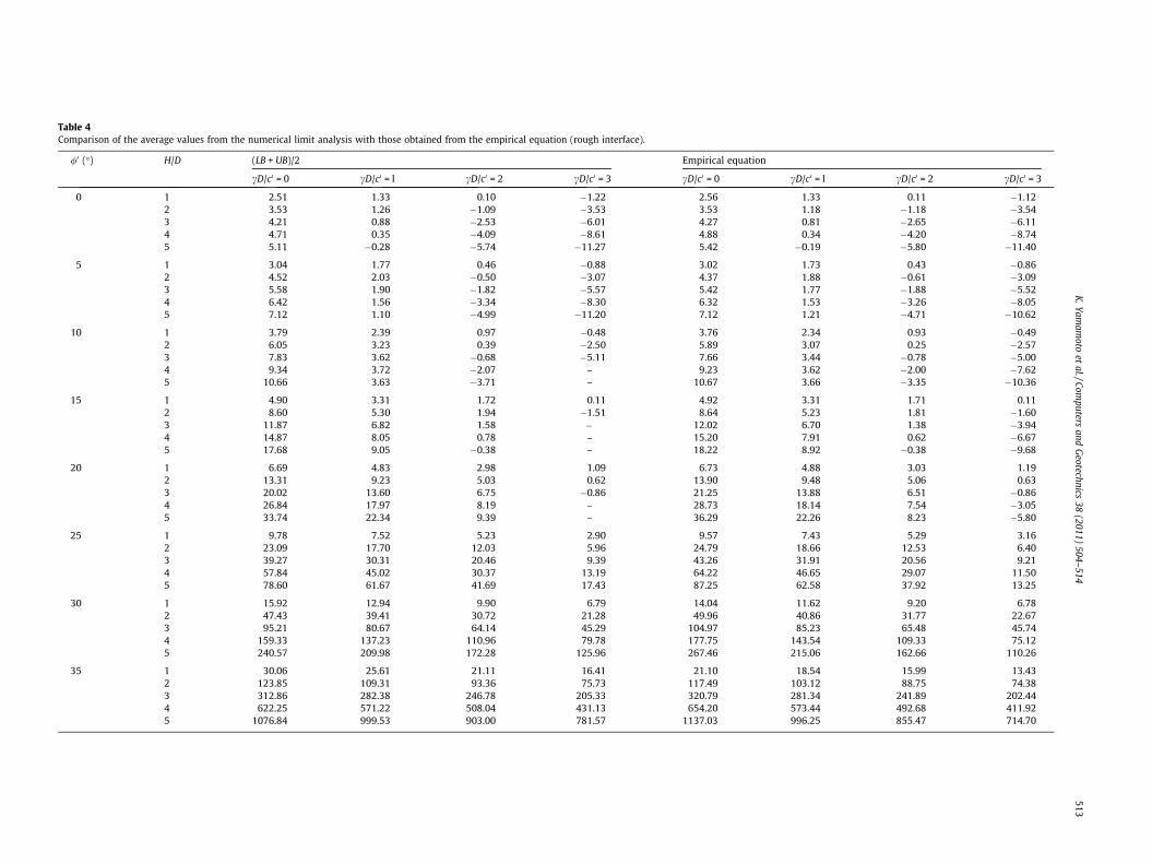
Table 4Comparison of the average values from the numerical limit analysis with those obtained from the empirical equation (rough interface).

/0 (�) H/D (LB + UB)/2 Empirical equation

cD/c0 = 0 cD/c0 = l cD/c0 = 2 cD/c0 = 3 cD/c0 = 0 cD/c0 = l cD/c0 = 2 cD/c0 = 3

0 1 2.51 1.33 0.10 �1.22 2.56 1.33 0.11 �1.122 3.53 1.26 �1.09 �3.53 3.53 1.18 �1.18 �3.543 4.21 0.88 �2.53 �6.01 4.27 0.81 �2.65 �6.114 4.71 0.35 �4.09 �8.61 4.88 0.34 �4.20 �8.745 5.11 �0.28 �5.74 �11.27 5.42 �0.19 �5.80 �11.40

5 1 3.04 1.77 0.46 �0.88 3.02 1.73 0.43 �0.862 4.52 2.03 �0.50 �3.07 4.37 1.88 �0.61 �3.093 5.58 1.90 �1.82 �5.57 5.42 1.77 �1.88 �5.524 6.42 1.56 �3.34 �8.30 6.32 1.53 �3.26 �8.055 7.12 1.10 �4.99 �11.20 7.12 1.21 �4.71 �10.62

10 1 3.79 2.39 0.97 �0.48 3.76 2.34 0.93 �0.492 6.05 3.23 0.39 �2.50 5.89 3.07 0.25 �2.573 7.83 3.62 �0.68 �5.11 7.66 3.44 �0.78 �5.004 9.34 3.72 �2.07 – 9.23 3.62 �2.00 �7.625 10.66 3.63 �3.71 – 10.67 3.66 �3.35 �10.36

15 1 4.90 3.31 1.72 0.11 4.92 3.31 1.71 0.112 8.60 5.30 1.94 �1.51 8.64 5.23 1.81 �1.603 11.87 6.82 1.58 � 12.02 6.70 1.38 �3.944 14.87 8.05 0.78 – 15.20 7.91 0.62 �6.675 17.68 9.05 �0.38 – 18.22 8.92 �0.38 �9.68

20 1 6.69 4.83 2.98 1.09 6.73 4.88 3.03 1.192 13.31 9.23 5.03 0.62 13.90 9.48 5.06 0.633 20.02 13.60 6.75 �0.86 21.25 13.88 6.51 �0.864 26.84 17.97 8.19 – 28.73 18.14 7.54 �3.055 33.74 22.34 9.39 – 36.29 22.26 8.23 �5.80

25 1 9.78 7.52 5.23 2.90 9.57 7.43 5.29 3.162 23.09 17.70 12.03 5.96 24.79 18.66 12.53 6.403 39.27 30.31 20.46 9.39 43.26 31.91 20.56 9.214 57.84 45.02 30.37 13.19 64.22 46.65 29.07 11.505 78.60 61.67 41.69 17.43 87.25 62.58 37.92 13.25

30 1 15.92 12.94 9.90 6.79 14.04 11.62 9.20 6.782 47.43 39.41 30.72 21.28 49.96 40.86 31.77 22.673 95.21 80.67 64.14 45.29 104.97 85.23 65.48 45.744 159.33 137.23 110.96 79.78 177.75 143.54 109.33 75.125 240.57 209.98 172.28 125.96 267.46 215.06 162.66 110.26

35 1 30.06 25.61 21.11 16.41 21.10 18.54 15.99 13.432 123.85 109.31 93.36 75.73 117.49 103.12 88.75 74.383 312.86 282.38 246.78 205.33 320.79 281.34 241.89 202.444 622.25 571.22 508.04 431.13 654.20 573.44 492.68 411.925 1076.84 999.53 903.00 781.57 1137.03 996.25 855.47 714.70

K.Yam

amoto

etal./Com

putersand

Geotechnics

38(2011)

504–514

513


solutions quite accurately, being to within 5% for all the values of H/D and /0 considered.

6. Conclusions

The stability of a plane strain circular tunnel, in a cohesive-frictional soil subjected to surcharge loading, has been investigatedusing upper-bound rigid-block analysis and finite element limitanalysis. The results of these analyses have been presented in theform of dimensionless stability charts. The lower and upper-bounds obtained using finite element limit analysis bracket theactual ultimate surcharge load to within ±6% or better. As anadditional check of the validity of the finite element limit analysisresults, several upper-bound rigid-block mechanisms were devel-oped. A comparison of the upper-bound solutions obtained fromthe rigid-block analysis with those of finite element limit analysisshows good agreement when /0 and H/D are small. An empiricalequation for estimating the ultimate surcharge load that can beapplied to the surface of a cohesive-frictional soil above a shallowcircular tunnel has been proposed. This equation is based onaverage values of the lower- and upper-bound solutions from finiteelement limit analysis, and predicts these values to within 5%.

References

[1] Lyamin AV, Sloan SW. Lower bound limit analysis using non-linearprogramming. Int J Numer Meth Eng 2002;55:573–611.

[2] Krabbenhøft K, Lyamin AV, Hjiaj M, Sloan SW. A new discontinuous upperbound limit analysis formulation. Int J Numer Meth Eng 2005;63:1069–88.

[3] Cairncross AM. Deformation around model tunnels in stiff clay. PhD thesis.University of Cambridge; 1973.

[4] Atkinson JH, Cairncross AM. Collapse of a shallow tunnel in a Mohr-Coulombmaterial. In: Role of plasticity in soil mechanics, Cambridge; 1973. p. 202–06.

[5] Mair RJ. Centrifugal modelling of tunnel construction in soft clay. PhD thesis.University of Cambridge; 1979.

[6] Seneviratne HN. Deformations and pore-pressures around model tunnels insoft clay. PhD thesis. University of Cambridge; 1979.

[7] Davis EH, Gunn MJ, Mair RJ, Seneviratne HN. The stability of shallow tunnelsand underground openings in cohesive material. Geotechnique 1980;30(4):397–416.

[8] Muhlhaus HB. Lower bound solutions for circular tunnels in two and threedimensions. Rock Mech Rock Eng 1985;18:37–52.

[9] Leca E, Dormieux L. Upper and lower bound solutions for the face stability ofshallow circular tunnels in frictional material. Geotechnique 1990;40(4):581–606.

[10] Sloan SW, Assadi A. Stability of shallow tunnels in soft ground. In: Holsby GT,Schofield AN, editors. Predictive soil mechanics. London: Thomas Telford;1993. p. 644–63.

[11] Lyamin AV, Sloan SW. Stability of a plane strain circular tunnel in a cohesive-frictional soil. In: Proceedings of the J.R. Booker Memorial symposium, Sydney;2000. p. 139–53.

[12] Yamamoto K, Lyamin AV, Sloan SW, Abbo AJ. Bearing capacity of a cohesive-frictional soil with a shallow tunnel. In: Proc. 13th Asian regional conf on soilmechanics and geotech eng, vol. 1, Kolkata; 2007. p. 489–92.

[13] Sloan SW. Lower bound limit analysis using finite elements and linearprogramming. Int J Numer Analyt Meth Geomech 1988;12:61–77.

[14] Sloan SW. Upper bound limit analysis using finite elements and linearprogramming. Int J Numer Analyt Meth Geomech 1989;13:263–82.

[15] Sloan SW, Kleeman PW. Upper bound limit analysis using discontinuousvelocity fields. Comput Methods Appl Mech Eng 1995;127:293–314.

[16] Chen WF. Limit analysis and soil plasticity. Amsterdam: Elsevier; 1975.[17] Bunday BD. Basic optimisation methods. Edward Arnold; 1984.

Documents

Stability of a circular tunnel in cohesive-frictional soil ... of a circular tunnel in cohesive-frictional ... Six types of rigid-block mechanisms were constructed, as shown ... frictional