Stability of the SABR model - Deloitte US · Stability of the SABR model | Factors affecting stability 05 Discontinuities in the forward rate curve One of the parameters in the SABR

00

Stability of the SABR model October 2016

Stability of the SABR model | Contents

01

Contents

Contents 1

Introduction 3

Factors affecting stability 4

Stability of SABR parameters 7

Calibration space 13

How we can help 16

Contacts 17

02

This article investigates the stability of the SABR parameters across a range of historical data. It describes some of the various factors that can affect the stability in both the Black and Normal calibration spaces.

Stability of the SABR model | Contents

Stability of the SABR model | Introduction

03

Introduction Since its inception the SABR model has become the dominant market model for interest-rate derivatives. It owes its popularity to two main factors: Firstly, it models both the underlying forward rate and its volatility. This is an essential element in order for any model to reproduce the volatility smile. The second element is the derivation by Hagan et al of an approximate closed-form formula for the implied volatility in terms of the four SABR parameters. This is a key ingredient for quick calibration of the model to the market.

The closed form SABR formulas1, however, come with a number of disadvantages. A well-known weakness is the fact that the probability density function of the forward rate becomes negative for very low strikes. This is an artefact of the various asymptotic expansions that lead to the closed-form formula. This weakness becomes particularly important in the current negative-rate environment where derivatives are traded at negative or low strikes. The literature in the area of “fixing” the SABR model is quite rich, ranging from “quick and dirty”-type solutions, where a reasonably-behaving tail is attached to the body of the SABR PDF, to more elaborate variations of the SABR model.

For risk-management purposes a common question concerning the SABR model is about the stability of its parameters: An undesirable feature would be to have jumps in the SABR parameters across expiries or across valuation dates which would trigger other risk-management actions.

In this document, we present some visualizations concerning the evolution of the parameters. We also compare two versions of the SABR model encountered in practice, one that fixes the parameter beta to a positive value (typically to beta=1/2) and a second one that fixes beta to the value of zero.

1 See, for example, Hagan et al “Managing Smile Risk” Wilmott Magazine (7/2002), or, Berestycki et al. “Computing the implied volatility in stochastic volatility models” Comm. Pure Appl. Math., 57 1352, 2004

Stability of the SABR model | Factors affecting stability

04

Factors affecting stability The SABR model carries four parameters (alpha, beta, rho, nu). According to common market practice the parameter beta is fixed to a certain value while the optimisation is run on the remaining three. The calibration error in the SABR model can be measured by, e.g. the sum of square errors between the market vols and the model vols.

The stability of the SABR model is affected by a series of factors some of which are:

The number of local minima in the error surface The SABR error surface that is generated in the space of (alpha, rho, nu) is described by a large number of local minima. In the two figures below we illustrate the location and depth of various local minima.

The size of the bubbles in these figures is inversely-proportional to the depth of the error surface, i.e. a large bubble would imply a small error. In these figures we see that global minimum of the SABR error surface is surrounded by a significant number of local minima (these figures are generated from the calibration of the EUR6M tenor as of 31 August 2016 on the 4YR expiry). As a result of this, a non-stochastic optimization algorithm may be trapped and not converge to the global optimum solution. Stochastic optimisation algorithms such as simulated annealing or genetic algorithms offer the advantage that at every new iteration step in the procedure they propose a move to a seemingly unfavourable location. This, however, offers the advantage that they can escape from local minima. Non-stochastic algorithms such as gradient descent or Levenberg-Marquardt do not offer this feature, although one way to incorporate stochasticity into the search would be to restart the optimiser from different initial conditions.

Because of the large number of local minima in the error surface, the convergence of the algorithm to different solutions may impact the smoothness of the SABR parameters.


05

Discontinuities in the forward rate curve One of the parameters in the SABR formula is the forward rate. The term structure of the forward rate is usually bootstrapped from other market instruments. There is a certain number of choices that can be made in this procedure, for example, linear-interpolations versus spline-interpolations or interpolations in the spot-rate versus interpolations on the discount-curve, etc. Although all of these options are valid (as long as the price of the market instruments is reproduced correctly) they can lead to different behaviours of the forward curve and therefore different behaviours of the SABR parameters. The impact of this choice of the forward rate on the MTM can be quantified as a fraction of the Delta sensitivity.

An example of a forward curve built on two different interpolation assumptions is shown below.

Caplet stripping The SABR formula expresses the implied caplet volatility in terms of the SABR parameters. However, caplet vols are not immediately quoted in the market. Rather, it is cap vols that are quoted, mainly for efficiency reasons. As a result of this unavailability, caplet vols need to be generated from the cap vols. There is no unique way to do this and there are various possible options that are all valid as long as the input market instruments are repriced correctly. The simplest possible approach would be to assume that caplet vols that fall between two quoted cap expiries are equal. This would be the “flat” interpolation. More elaborate assumptions would be to assume some term-structure of the caplet vols in-between expiries. The figure below illustrates schematically this difference.

The blue markers correspond to the “flat” caplet vol assumption while the green markers to an interpolation scheme.

-0,5

0

0,5

1

1,5

22-09-17 20-09-27 17-09-37 15-09-47

FORW

ARD

RAT

E

DATE

EUR6M FWD 31 AUG 16

Piecewise Linear

Smooth Interpolation

Caplet vols

Time

6M 1Y 2Y 18M


06

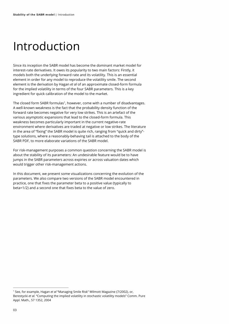
In the figure below we illustrate an example of caplet stripping. This example assumes a flat interpolation and is done on the EUR 6M tenor as of 31 August 2016. The figure shows that differences in caplet vols are not significant and thus we do not expect the flat interpolation assumption to play a big role in the stability of the SABR parameters. The impact on the MTM can be quantified in terms of the Vega sensitivity.

0,10

0,12

0,14

0,16

0,18

0,20

0,22

0,24

0,26

- 5,00 10,00 15,00 20,00

EXPIRY (YR)

Black Caplet Vols

Stability of the SABR model | Stability of SABR parameters

07

Stability of SABR parameters In order to examine the stability of the SABR parameters, we have calibrated the shifted SABR model on the EUR 6M cap market for a series of end-of-month valuation dates, from 31 August 2015 to 31 August 2016. For each of these valuation dates we have obtained the input normal cap vols from Bloomberg for a range of strikes from 1% to 11% (and also including the ATM point) and for a range of maturities from 1YR to 25YR.

The figures below show the calibrated values of alpha, rho and nu obtained in the shifted Black calibration space with a shift of 2% and a value of beta fixed to 0.5.

The various lines in the figures correspond to calibrations at different valuation dates. These figures show that the values of the three parameters do not fluctuate significantly. Alpha, Rho and Nu each follow a main trending curve.


08

An alternative way to view these results is to isolate certain expiries and plot the values of the parameters against the valuation dates. This can be seen in the figure below:

On the horizontal axis we find the 14 valuation dates and on the vertical axis the value of the SABR parameter for the 1YR and 5YR expiries. From here we see that across valuation dates the deviation is not significant. There are certain isolated instances where the values jump (for example, on the 31 December 2015 valuation) but this may have roots linked to end-of-year closing trades.

In order to smoothen further the calibration results, one could regress the obtained results, either across expiries or across valuation dates. A regression across valuation dates could also be used in order to forecast the values of the SABR parameters at a future valuation date or in order to make an educated guess of the appropriate initial conditions of the optimiser at a future valuation date.


09

We have applied a linear regression of 5th order across the expiries for each of the valuation dates. The particular order of the applied regression is not very important, as long as one does not overfit. The result is shown in the figure below:

With the regression results at hand one would now be tempted to quantify the stability of the SABR parameters by examining how much cap prices would differ using a pricing based on (i) the raw calibrated parameters versus (ii) the regressed parameters. If the SABR model were stable then one would expect that the regressed cap prices would not differ much from the calibrated ones.


10

The results of this test are shown in the three tables below.

The first table shows the values of cap prices using as valuation date 29 February 2015 (a middle date in the pool). They have been obtained via a simple conversion of the raw Bloomberg cap vols using a Black formula. Hence this can be considered as the reference table.

CAP PRICES

BLOOMBERG

Tenor ATM K ATM 1.00% 1.50% 2.00% 2.50% 3.00%

1Yr -0.24% 10,134 15.794 4.207 1.455 0.597 0.278

2Yr -0.24% 28,171 1,323 709 436 293 210

3Yr -0.19% 56,001 7,526 4,384 2,814 1,941 1,410

4Yr -0.11% 97,871 24,683 15,403 10,273 7,230 5,310

5Yr -0.02% 157,913 56,774 37,272 25,650 18,391 13,663

6Yr 0.09% 236,309 108,035 73,170 51,174 36,954 27,481

7Yr 0.21% 324,995 178,480 124,930 89,698 66,209 50,195

8Yr 0.33% 424,746 267,137 191,078 138,916 103,127 78,270

9Yr 0.44% 529,501 369,584 269,691 199,124 149,605 114,667

10Yr 0.54% 637,762 482,560 358,086 268,318 204,174 158,226

The second and third tables (below) show the cap price values obtained by using the raw calibrated SABR parameters vs the regressed SABR parameters. Taking into account that the notional considered in this test was 10 mio EUR implies that the absolute difference in the cap prices between regressed vs calibrated is a mere 0.85 basis points. This is an acceptable difference.

CALIBRATED

SABR

Tenor ATM K ATM 1.00% 1.50% 2.00% 2.50% 3.00%

1Yr -0.24% 10,195 16.591 4.130 1.334 0.514 0.226

2Yr -0.24% 28,029 1,330 727 452 305 219

3Yr -0.19% 55,958 7,407 4,361 2,834 1,975 1,447

4Yr -0.11% 97,378 24,753 15,625 10,520 7,447 5,484

5Yr -0.02% 157,680 57,149 37,778 26,112 18,756 13,920

6Yr 0.09% 235,448 108,294 73,533 51,436 37,090 27,526

7Yr 0.21% 324,301 178,503 124,938 89,490 65,814 49,697

8Yr 0.33% 424,425 267,962 191,834 139,128 102,736 77,436

9Yr 0.44% 529,564 370,988 271,217 200,066 149,754 114,121

10Yr 0.54% 636,905 483,057 359,234 269,166 204,412 157,899


11

REGRESSED

SABR

Tenor ATM K ATM 1.00% 1.50% 2.00% 2.50% 3.00%

1Yr -0.24% 9,988 13.802 3.510 1.161 0.459 0.206

2Yr -0.24% 28,520 1,389 729 435 284 196

3Yr -0.19% 57,015 8,183 4,865 3,172 2,208 1,615

4Yr -0.11% 99,462 25,268 15,922 10,752 7,662 5,692

5Yr -0.02% 159,313 56,370 36,941 25,480 18,361 13,721

6Yr 0.09% 234,096 106,018 71,978 50,658 36,896 27,711

7Yr 0.21% 323,307 177,465 124,501 89,477 65,983 49,897

8Yr 0.33% 422,305 266,779 192,054 140,494 104,786 79,783

9Yr 0.44% 528,115 370,795 272,543 202,482 152,677 117,117

10Yr 0.54% 637,571 484,946 362,325 272,693 207,661 160,483

An alternative way to visualise the co-movement of the three parameters across expiries is to plot them against each other. The figure below shows (alpha,rho), (nu,rho) and (alpha, nu) for all calibrations in the 13 valuation dates. These calibrations have been done on the EUR 6M cap market using the Black asymptotic formula with a shift of 2% and beta=1/2. The various expiries are shown in different colors.


12

In the left picture we see that optimum solution moves from left (red) to right (magenta). While the optimal solution for the various valuation dates appear somewhat scattered in the first expiries, they settle down to more localised regions towards the final expiries. This is to be expected: the market view for the first expiries is much clearer than that of the last expiries. We also see that as expiry progresses from 1YR to 25YR the alphas tend to increase while the rhos tend to somewhat decrease. This can be appreciated on the basis that alphas are linked to ATM vols while rhos are linked to the skew. As expiry increases, the term-structure of the ATM vols shows an increase while the smile flattens out. At the same time, the second figure shows that the value of the parameter nu decreases. This is indicative of the loss in convexity of the caplet smile, as expiries go from 1YR to 25YR.

Stability of the SABR model | Calibration space

13

Calibration space The SABR model expresses the implied volatility either in terms of a Black volatility (which will be input to a Black’76 formula) or in terms of a Normal volatility (which will be input to a Bachelier formula). In recent years, with the interest-rates going into the negative domain there has been an obvious obstacle in any Black pricing engine: the Black formula requires the computation of the logarithm of the forward and of the strike, which, if negative, leads to an unpleasant exception error.

One quick fix to this problem is to shift both the forward and the strike so that the logarithm is not undefined. This then leads to a new model, the shifted SABR model. The asymptotic expansions of Hagan et. al. and Berestycki et. al.2 can easily be adapted in order to deal with this shift. In a Black world, these formulas would no longer yield the common Black volatility, rather, they quote a shifted Black volatility. In the Normal world, the Hagan asymptotic expansion will yield a Normal volatility (note that in the Bachelier formula, the shift on the strike and the shift on the forward will cancel each other out, meaning that there is no impact of a shift on a normal model). Calibration of the SABR model using a shifted Black SABR asymptotic formula would be called the “(shifted) Black calibration space”, whereas a calibration using the Normal asymptotic formula is called the “Normal calibration space”.

Black Calibration Space

,1

124

11920 ⋯

∙

∙ 1124

14

2 324

∙ ⋯

where and are abbreviations of

1 21

2 Hagan et al “Managing Smile Risk” Wilmott Magazine (7/2002) and Berestycki et al. “Computing the implied volatility in stochastic volatility models” Comm. Pure Appl. Math., 57 1352, 2004


14

Normal Calibration Space

,1

124

11920 ⋯

1124

11920 ⋯

∙

∙ 1224

14

2 324

∙ ⋯

These expressions hold for any value of beta. Notice that a shift is necessary (due to the presence of logarithms of the strike and forward) in either the Black or the Normal calibration space.

The Hagan et al article derives in the special case of beta=0 a convenient expression for the normal implied vol3. The expression in the Normal beta=0 case contains no logarithms and can thus be used, in the presence of negative strikes or forwards, without the need to introduce a shift. This implies that there is no need for laborious software adaptations apart from fixing the parameter beta to the value of zero, provided the pricing library can already handle a calibration in the beta=0 Normal space.

There is a certain amount of discussion in the literature and among market dealers of whether a SABR model with beta=0 would be an appropriate model. This is because setting beta equal to zero in the SABR model would lead to a stochastic differential equation for the forward whereby the increments to the forward rate do not depend on its current value. This is, from a phenomenological point of view, a problematic issue, although, from a pricing point of view, all that matters to a model is its calibration to the observed market prices.

The question that then rises is whether the Normal beta=0 model (without a shift) is as appropriate as the shifted beta>0 model, in terms of stability. In order to provide some indicative answers to this question we have calibrated the pool of EUR6M historical data in both the shifted Black calibration space (with beta=0.5 and shift=2%) and in the Normal calibration space (with beta=0 and shift=0%).

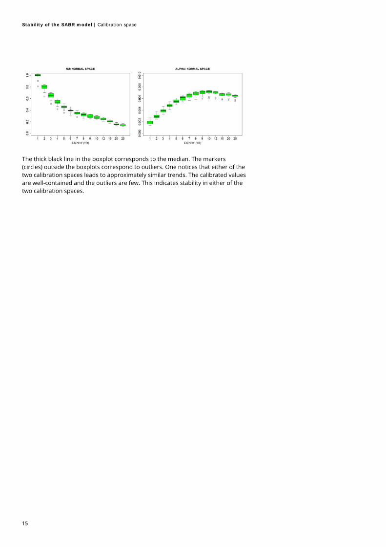
The results are presented in the figures below which show boxplots across all expiries for both calibration spaces. Each of the boxplots contain 50% of the calibration data for all valuation dates for each expiry.

3 The reader is warned that the normal beta=0 formula in the Hagan et al paper contains a typo error.


15

The thick black line in the boxplot corresponds to the median. The markers (circles) outside the boxplots correspond to outliers. One notices that either of the two calibration spaces leads to approximately similar trends. The calibrated values are well-contained and the outliers are few. This indicates stability in either of the two calibration spaces.

Stability of the SABR model | How we can help

16

How we can help Our team of quants provides assistance at various levels of the pricing process, from training to design and implementation.

Deloitte’s option pricer is used for Front Office purposes or as an independent validation tool for Validation or Risk teams.

Some examples of solutions tailored to your needs:

A managed service where Deloitte provides independent valuations of vanilla interest rate produces (caps, floors, swaptions, CMS) at your request.

Expert assistance with the design and implementation of your own pricing engine.

A stand-alone tool. Training on the SABR model, the shifted methodology, the volatility smile,

stochastic modelling, Bloomberg or any other related topic tailored to your needs.

The Deloitte Valuation Services for the Financial Services Industry offers a wide range of services for pricing and validation of financial instruments.

Why our clients haven chosen Deloitte for their Valuation Services:

Tailored, flexible and pragmatic solutions Full transparency High quality documentation Healthy balance between speed and accuracy A team of experienced quantitative profiles Access to the large network of quants at Deloitte worldwide Fair pricing

Stability of the SABR model | Contacts

17

Contacts Nikos Skantzos Director Diegem

T: +32 2 800 2421 M: + 32 474 89 52 46 E: [email protected]

Kris Van Dooren Senior Manager Diegem

T: +32 2 800 2495 M: + 32 471 12 78 81 E: [email protected]

George Garston Senior Consultant Zurich (Switzerland)

T: +41 58 279 7199 E: [email protected]

Stability of the SABR model | Contacts

18

Deloitte refers to one or more of Deloitte Touche Tohmatsu Limited, a UK private company limited by guarantee (“DTTL”), its network of member firms, and their related entities. DTTL and each of its member firms are legally separate and independent entities. DTTL (also referred to as “Deloitte Global”) does not provide services to clients. Please see www.deloitte.com/about for a more detailed description of DTTL and its member firms. Deloitte provides audit, tax and legal, consulting, and financial advisory services to public and private clients spanning multiple industries. With a globally connected network of member firms in more than 150 countries, Deloitte brings world-class capabilities and high-quality service to clients, delivering the insights they need to address their most complex business challenges. Deloitte has in the region of 225,000 professionals, all committed to becoming the standard of excellence. This publication contains general information only, and none of Deloitte Touche Tohmatsu Limited, its member firms, or their related entities (collectively, the “Deloitte Network”) is, by means of this publication, rendering professional advice or services. Before making any decision or taking any action that may affect your finances or your business, you should consult a qualified professional adviser. No entity in the Deloitte Network shall be responsible for any loss whatsoever sustained by any person who relies on this publication. © October 2016 Deloitte Belgium

Documents

Stability of the SABR model - Deloitte US · Stability of the SABR model | Factors affecting stability 05 Discontinuities in the forward rate curve One of the parameters in the SABR