HAL Id: tel-00745915https://tel.archives-ouvertes.fr/tel-00745915

Submitted on 26 Oct 2012

HAL is a multi-disciplinary open accessarchive for the deposit and dissemination of sci-entific research documents, whether they are pub-lished or not. The documents may come fromteaching and research institutions in France orabroad, or from public or private research centers.

L’archive ouverte pluridisciplinaire HAL, estdestinée au dépôt et à la diffusion de documentsscientifiques de niveau recherche, publiés ou non,émanant des établissements d’enseignement et derecherche français ou étrangers, des laboratoirespublics ou privés.

Stability of Transfermium Elements at High Spin :Measuring the Fission Barrier of 254No

Gregoire Henning

To cite this version:Gregoire Henning. Stability of Transfermium Elements at High Spin : Measuring the Fission Bar-rier of 254No. Other [cond-mat.other]. Université Paris Sud - Paris XI, 2012. English. NNT :2012PA112143. tel-00745915

!"#$%&'#(%)*+&#','!-

./01%)-0/(0&+1%)2)!"#$%&'()*+,-./"'0,)$,1.*2.*13456375869)2)/9:769);9)'<9=765>?7689)"@=A?3869)97);9)'<9=765>?7689);9)B3CC9

!"#$"%&"'()3,!4/*%5'),-'&(6"%#)

!"#$%&'%&'()!(*+!

C5@79:@9)A9)DE)'9<79>469)DEFD

<36

,-./&"%0010,

'7348A87G)5H)(63:CH96>8@>)%A9>9:7C)37)I8JK)'<8:2)B93C@68:J)7K9)L8CC85:)M366896)5H)DNO"5

'2-.34.5-&6.&4789.&: &&&&&&&&&&& +-;3.<2&=>?.@AB;-4.C9 /K36J?9);9)69=K96=K9)P/'"'BQ)>A62-.34.5-&6.&4789.&:) (9:J,19R)SK55) -869=79@6);9)69=K96=K9)P7#8.99),-"$%.9"(,:";<=

)>D?>9242>C&65&E5-F&:

!#6*%>)9$,>',?'#/,3, %A83C)SI+" *65H9CC9@6)P#*")06C3GQ@"AA.#$)'#*,3,, '8AT83)195:8 *65H9CC9@69)P-8<3678>9:75);8)L8C8=3U)

)))))!:8T96C873);8)B8A3:5Q*9796)&89796 *65H9CC9@6)P#:C787@7)H@96)S96:<KGC8RU)

))))!:8T96C87397)V@)S59A:QB0"2%9"$)'#,3, )))))))))) *K8A8<<9)W!%"(#" *65H9CC9@6).>?6879)P/%"MXQ

2

Abstract

Super heavy nuclei provide opportunities to study nuclear struc-

ture near three simultaneous limits: in charge Z, spin I and excita-

tion energy E∗. These nuclei exist only because of a fission barrier,

created by shell effects. It is therefore important to determine the

fission barrier and its spin dependence Bf(I), which gives informa-

tion on the shell energy Eshell(I). Theoretical calculations predict

different fission barrier heights from Bf(I = 0) = 6.8 MeV for a

macro-microscopic model [1, 2] to 8.7 MeV for Density Functional

Theory calculations using the Gogny or Skyrme interactions [3–5].

Hence, a measurement of Bf provides a test for theories.

To investigate the fission barrier, an established method is to

measure the rise of fission with excitation energy, characterised by

the ratio of decay widths Γfission/Γtotal, using transfer reactions [6,7].

However, for heavy elements such as 254No, there is no suitable tar-

get for a transfer reaction. We therefore rely on the complementary

decay widths ratio Γγ/Γfission and its spin dependence, deduced from

the entry distribution (I, E∗).

Measurements of the gamma-ray multiplicity and total energy for254No have been performed with beam energies of 219 and 223 MeV

in the reaction 208Pb

48Ca, 2n

at ATLAS (Argonne Tandem Linac

Accelerator System). The 254No gamma rays were detected using

the Gammasphere array as a calorimeter – as well as the usual high-

resolution γ-ray detector. Coincidences with evaporation residues

at the Fragment Mass Analyzer focal plane separated 254No gamma

rays from those from fission fragments, which are > 106 more in-

tense. From this measurement, the entry distribution – i.e. the

initial distribution of I and E∗ – is constructed. Each point (I, E∗)

of the entry distribution is a point where gamma decay wins over

3

fission and, therefore, gives information on the fission barrier.

The measured entry distributions show an increase in the max-

imum spin and excitation energy from 219 to 223 MeV of beam

energy. The distributions show a saturation of E∗ for high spins.

The saturation is attributed to the fact that, as E∗ increases above

the saddle, Γfission rapidly dominates. The resulting truncation of

the entry distribution at high E∗ allows a determination of the fis-

sion barrier height.

The experimental entry distributions are also compared with en-

try distributions calculated with decay cascade codes which take

into account the full nucleus formation process, including the cap-

ture process and the subsequent survival probability as a function

of E∗ and I. We used the KEWPIE2 [8] and NRV [9] codes to sim-

ulate the entry distribution.

4

Stabilité des Éléments Trans-fermium à Haut Spin :Mesure de la Barrière de Fission de 254No

Les noyaux super lourds offrent la possibilité d’étudier la structure

nucléaire à trois limites simultanément: en charge Z, spin I et énergie

d’excitation E∗. Ces noyaux existent seulement grâce à une barrière

de fission créée par les effets de couche. Il est donc important de

déterminer cette barrière de fission et sa dépendance en spin Bf(I),

qui nous renseigne sur l’énergie de couche Eshell(I). Les théories

prédisent des valeurs différentes pour la hauteur de la barrière de

fission, allant de Bf(I = 0) = 6.8 MeV dans un modèle macro-

microscopique [1, 2] à 8.7 MeV pour des calculs de la théorie de la

fonctionnelle de la densité utilisant l’interaction Gogny ou Skyrme

[3–5]. Une mesure de Bf fournit donc un test des théories.

Pour étudier la barrière de fission, la méthode établie est de

mesurer, par réaction de transfert, l’augmentation de la fission avec

l’énergie d’excitation, caractérisée par le rapport des largeurs de

décroissance Γfission/Γtotal, [6,7]. Cependant, pour les éléments lourds

comme 254No, il n’existe pas de cible appropriée pour une réaction

de transfert. Il faut s’en remettre à un rapport de largeur de décrois-

sance complémentaire: Γγ/Γfission et sa dépendance en spin, déduite

de la distribution d’entrée (I, E∗).

Des mesures de la multiplicité et l’énergie totale des rayons γ de254No ont été faites aux énergies de faisceau 219 et 223 MeV pour

la réaction 208Pb

48Ca, 2n

à ATLAS (Argonne Tandem Linac Ac-

celerator System). Les rayons γ du 254No ont été détectés par le

multi-détecteur Gammasphere utilisé comme calorimètre – et aussi

5

comme détecteur de rayons γ de haute résolution. Les coïncidences

avec les résidus d’évaporation au plan focal du Fragment Mass An-

alyzer ont permis de séparer les rayons γ du 254No de ceux issus

de la fission, qui sont > 106 fois plus intenses. De ces mesures, la

distribution d’entrée – c’est-à-dire la distribution initiale en I et E∗

– est reconstruite. Chaque point (I, E∗) de la distribution d’entrée

est un point où la décroissance γ l’a emporté sur la fission, et ainsi,

contient une information sur la barrière de fission.

La distribution d’entrée mesurée montre une augmentation du

spin maximal et de l’énergie d’excitation entre les énergies de fais-

ceau 219 et 223 MeV. La distribution présente une saturation de E∗

à hauts spins. Cette saturation est attribuée au fait que, lorsque

E∗ augmente au-dessus de la barrière, Γfission domine rapidement. Il

en résulte une troncation de la distribution d’entrée à haute énergie

qui permet la détermination de la hauteur de la barrière de fission.

La mesure expérimentale de la distribution d’entrée est également

comparée avec des distributions d’entrée calculées par des simula-

tions de cascades de décroissance qui prennent en compte le pro-

cessus de formation du noyau, incluant la capture et la survie, en

fonction de E∗ et I. Dans ce travail, nous avons utilisé les codes

KEWPIE2 [8] et NRV [9] pour simuler les distributions d’entrée.

6

7

8

On a qu’à parler avec une robe et un bonnet, tout galimatias

devient savant, et toute sottise devient raison.

MolièreLe Malade imaginaire, Acte III, Scène 14.

10

Foreword

Reaching the end of those three years of work, I can say that I met a lot of great people. Ienjoyed working with them and in the process, gained colleagues and, dare I say, friends.

I first want to give the biggest thanks to my supervisors: Waely and Teng Lek. I couldnot have dreamed of anybody better to help me during those three years. They let me allthe autonomy I needed to work while guiding me and being available for all my questions.

Thank you to Silvia Leoni and Peter Reiter for accepting to review my (long) manuscriptduring the summer. Thanks to Philippe Quentin for being part of the defense jury and toElias Khan for presiding it. I am grateful to all the jury members who asked challengingquestions and provided insightful comments that will help move the analysis to even moresignificant results.

Thanks to David Potterveld for helping with the experiment data that would have beenlost without him. Thank you to Darek Seweryniak, Mike Carpente, Torben Lauritsenand Shaofei Zhu for their support and involvement in the experiment and the analysis.Thank you to Neil Rowley and David Boiley for their interest in my work and fruitfuldiscussions. Thank you to Peter Reiter for providing many information on the previousexperiment. Thanks to Andreas Heinz, with whom I learnt a lot about nuclear physics,and who provided comments and encouragement.

I thank all my colleagues at Argonne National Lab.: Andrew, Ben, Birger, Calem, Chris,Chitra, Darek, David, Filip, Gulan, Kim, Libby, Martin, Mike, Peter, Robert and Shaofei,and at CSNSM: Carole, Catherine, Dave, Georges, Georgi, Joa, Karl, Pierre and Stephanieand specially my office-mates and fellow thésards : Asenath, Asli, Cédric, Christophe, Meng.Thank you to the administrative staff: Annie, Christine, Patricia, Réjane and Sonia inOrsay and Coleen, Barbara and Janet at Argonne, for their essential support.

I can’t forget the other student from NPAC 2009 class, in particular, the happy few nuclearphysicists among them: Aurore and Fabien.

Last but certainly not least, from the bottom of my heart, I thank Corinne for all she didfor me.

11

Collaborators

This work was possible with the help of : T. L. Khoo1, A. Lopez-Martens2, D. Seweryniak1,M. Alcorta1, M. Asai3, B. B. Back1, P. Bertone1, D. Boiley4, M. P. Carpenter1, C. J. Chiara1,5,P. Chowdhury6, B. Gall7, P. T. Greenlees8, G. Gurdal9, K. Hauschild2, A. Heinz10, C. R. Hoffman1,R. V. F. Janssens1, A. V. Karpov11, B. P. Kay1, F. G. Kondev1, S. Lakshmi6, T. Lauristen1,C. J. Lister6, E. A. McCutchan12, C. Nair1, J. Piot4, D. Potterveld1, P. Reiter13, N. Rowley14,A. M. Rogers1 and S. Zhu1.

1 Argonne National Laboratory,Argonne, IL, USA

2 CSNSM, IN2P3-CNRS, Orsay, France

3 Japan Atomic Energy Agency (JAEA), Japan

4 GANIL, CEA-DSM and IN2P3-CNRS, B.P. 55027, F-14076 Caen Cedex, France

5 University of Maryland, College Park, MD, USA

6 University of Massachusetts Lowell, Lowell, MA, USA

7 IPHC, IN2P3-CNRS and Universite Louis Pasteur, F-67037 Strasbourg Cedex 2, France

8 University of Jyväskylä, Finland

9 DePaul University, Chicago, IL

10 Fundamental Fysik, Chalmers Tekniska Hogskola, 412 96 Goteborg, Sweden

11 Flerov Laboratory of Nuclear Reactions, JINR, Dubna, Moscow Region, Russia

12 Brookhaven National Lab., Brookhaven, NY

13 Universität zu Köln, Germany

14 IPNO, CNRS/IN2P3, Université Paris-Sud 11, F-91406 Orsay Cedex, France

This work is supported by the U.S. Department of Energy, under Contract Nos. DE-AC02-06CH11357, DE-FG02-91ER-40609 and DE-FG02-94ER40848

12

Contents

1 Introduction 21

1.1 Nuclear Landscape: toward the Island of stability . . . . . . . . . . . . . . 21

1.1.1 Discovering the nucleus . . . . . . . . . . . . . . . . . . . . . . . . . 21

1.1.2 The nuclear landscape today . . . . . . . . . . . . . . . . . . . . . . 24

1.1.3 From magic numbers to Super Heavy Elements . . . . . . . . . . . 28

1.1.4 Story of a very heavy nucleus: 254No . . . . . . . . . . . . . . . . . 29

1.1.5 Motivation for measuring the fission barrier of 254No . . . . . . . . . 29

1.2 Nuclear properties . . . . . . . . . . . . . . . . . . . . . . . . . . . . . . . 30

1.2.1 Macroscopic and ground state properties . . . . . . . . . . . . . . . 30

1.2.2 Excited states in the nuclei . . . . . . . . . . . . . . . . . . . . . . . 33

1.2.3 Decay modes . . . . . . . . . . . . . . . . . . . . . . . . . . . . . . 35

2 Synthesis of Super Heavy Elements 39

2.1 Fusion Evaporation Reactions . . . . . . . . . . . . . . . . . . . . . . . . . 39

2.1.1 Capture . . . . . . . . . . . . . . . . . . . . . . . . . . . . . . . . . 40

2.1.2 Compound Nucleus: Fusion and Formation . . . . . . . . . . . . . . 42

2.1.3 Evaporation . . . . . . . . . . . . . . . . . . . . . . . . . . . . . . . 43

2.1.4 Evaporation residue formation . . . . . . . . . . . . . . . . . . . . . 49

13

2.2 Hot and Cold Fusion . . . . . . . . . . . . . . . . . . . . . . . . . . . . . . 49

2.2.1 Cold fusion . . . . . . . . . . . . . . . . . . . . . . . . . . . . . . . 49

2.2.2 Hot fusion . . . . . . . . . . . . . . . . . . . . . . . . . . . . . . . . 50

2.2.3 The case of 254No . . . . . . . . . . . . . . . . . . . . . . . . . . . . 50

2.3 The importance of Fission . . . . . . . . . . . . . . . . . . . . . . . . . . . 52

2.3.1 The fission process . . . . . . . . . . . . . . . . . . . . . . . . . . . 52

2.3.2 Bf dependence on I . . . . . . . . . . . . . . . . . . . . . . . . . . . 53

2.3.3 Probing the fission barrier . . . . . . . . . . . . . . . . . . . . . . . 53

3 Theoretical calculations 57

3.1 Theoretical predictions of the fission barrier height and spin dependence . . 57

3.2 Entry distribution calculation . . . . . . . . . . . . . . . . . . . . . . . . . 59

3.2.1 Analytic width calculations . . . . . . . . . . . . . . . . . . . . . . 59

3.2.2 evapOR calculation . . . . . . . . . . . . . . . . . . . . . . . . . . . 59

3.2.3 KEWPIE2 . . . . . . . . . . . . . . . . . . . . . . . . . . . . . . . . 59

3.2.4 NRV calculation . . . . . . . . . . . . . . . . . . . . . . . . . . . . . 61

3.2.5 Calculations of entry distribution: results . . . . . . . . . . . . . . . 66

3.3 Conclusion on calculations . . . . . . . . . . . . . . . . . . . . . . . . . . . 72

4 Experimental measurement of Fission Barrier 73

4.1 Experimental setup . . . . . . . . . . . . . . . . . . . . . . . . . . . . . . . 73

4.1.1 Reaction . . . . . . . . . . . . . . . . . . . . . . . . . . . . . . . . . 73

4.1.2 Beam structure . . . . . . . . . . . . . . . . . . . . . . . . . . . . . 75

4.1.3 Beam spot . . . . . . . . . . . . . . . . . . . . . . . . . . . . . . . . 77

4.1.4 Target . . . . . . . . . . . . . . . . . . . . . . . . . . . . . . . . . . 77

14

4.1.5 Reset foil . . . . . . . . . . . . . . . . . . . . . . . . . . . . . . . . 77

4.1.6 Gammasphere . . . . . . . . . . . . . . . . . . . . . . . . . . . . . . 79

4.1.7 Fragment Mass Analyzer . . . . . . . . . . . . . . . . . . . . . . . . 82

4.1.8 Focal plane detectors . . . . . . . . . . . . . . . . . . . . . . . . . . 83

4.1.9 Trigger . . . . . . . . . . . . . . . . . . . . . . . . . . . . . . . . . . 84

4.2 Recoil and recoil decay tagging . . . . . . . . . . . . . . . . . . . . . . . . 87

4.3 Calorimetric measurement . . . . . . . . . . . . . . . . . . . . . . . . . . . 88

4.3.1 Principle of measurement . . . . . . . . . . . . . . . . . . . . . . . . 88

4.3.2 Partial loss of BGO and Ge signals . . . . . . . . . . . . . . . . . . 91

5 Data analysis 95

5.1 Calibration of detectors . . . . . . . . . . . . . . . . . . . . . . . . . . . . . 95

5.1.1 Gammasphere . . . . . . . . . . . . . . . . . . . . . . . . . . . . . . 95

5.1.2 DSSD calibration . . . . . . . . . . . . . . . . . . . . . . . . . . . . 102

5.2 Recoil selection at the focal plane . . . . . . . . . . . . . . . . . . . . . . . 106

5.2.1 Contaminants . . . . . . . . . . . . . . . . . . . . . . . . . . . . . . 106

5.2.2 254Norecoils . . . . . . . . . . . . . . . . . . . . . . . . . . . . . . . 107

5.2.3 Cuts and Selections . . . . . . . . . . . . . . . . . . . . . . . . . . . 107

5.3 Test reaction: 176Y b (48Ca, 4 − 5n)220,219

Th . . . . . . . . . . . . . . . . . . 112

5.3.1 Reaction and production cross section . . . . . . . . . . . . . . . . 112

5.3.2 γ and decay spectroscopy of 220Th . . . . . . . . . . . . . . . . . . . 112

5.4 Cross section . . . . . . . . . . . . . . . . . . . . . . . . . . . . . . . . . . 116

5.5 Prompt γ spectroscopy . . . . . . . . . . . . . . . . . . . . . . . . . . . . . 117

5.6 Alpha spectroscopy . . . . . . . . . . . . . . . . . . . . . . . . . . . . . . . 120

15

5.6.1 Decay chain . . . . . . . . . . . . . . . . . . . . . . . . . . . . . . . 120

5.6.2 Decay energy and time . . . . . . . . . . . . . . . . . . . . . . . . . 122

5.7 Isomer decays . . . . . . . . . . . . . . . . . . . . . . . . . . . . . . . . . . 125

5.8 Principle of calorimetric measurement and calibration . . . . . . . . . . . 127

5.8.1 Measured quantities . . . . . . . . . . . . . . . . . . . . . . . . . . 127

5.8.2 Fold and Energy calibration . . . . . . . . . . . . . . . . . . . . . . 127

5.8.3 Response characteristics . . . . . . . . . . . . . . . . . . . . . . . . 133

5.9 The unfolding procedure . . . . . . . . . . . . . . . . . . . . . . . . . . . . 135

5.9.1 Principle of the unfolding . . . . . . . . . . . . . . . . . . . . . . . 136

5.9.2 Formal description of the unfolding . . . . . . . . . . . . . . . . . . 136

5.9.3 Validation of the unfolding . . . . . . . . . . . . . . . . . . . . . . . 138

5.10 Experimental Calorimetric measurements . . . . . . . . . . . . . . . . . . . 153

5.10.1 (k,H) distribution . . . . . . . . . . . . . . . . . . . . . . . . . . . . 153

5.10.2 Unfolding . . . . . . . . . . . . . . . . . . . . . . . . . . . . . . . . 155

5.10.3 Multiplicity to Spin and ESum to E∗ conversion . . . . . . . . . . . 155

5.11 Entry distribution . . . . . . . . . . . . . . . . . . . . . . . . . . . . . . . . 160

5.11.1 Comparison with previous measurement . . . . . . . . . . . . . . . 160

6 Entry distribution and fission barrier of 254No 165

6.1 Entry distribution: measurement and analysis . . . . . . . . . . . . . . . . 165

6.1.1 Measured unfolded distributions . . . . . . . . . . . . . . . . . . . . 165

6.1.2 Analysis of the Entry Distribution . . . . . . . . . . . . . . . . . . . 167

6.2 Extraction of the saddle energy . . . . . . . . . . . . . . . . . . . . . . . . 175

6.2.1 Fit on E1/2 . . . . . . . . . . . . . . . . . . . . . . . . . . . . . . . 175

16

6.2.2 Mapping the best parameters . . . . . . . . . . . . . . . . . . . . . 175

6.3 Conclusions on the Fission barrier . . . . . . . . . . . . . . . . . . . . . . . 179

6.3.1 Agreement with ∆(I) . . . . . . . . . . . . . . . . . . . . . . . . . . 179

6.3.2 Agreement with calculation . . . . . . . . . . . . . . . . . . . . . . 180

7 Perspectives 183

7.1 Measurement improvement: digital electronics . . . . . . . . . . . . . . . . 183

7.2 Neutron effect . . . . . . . . . . . . . . . . . . . . . . . . . . . . . . . . . . 183

7.3 Complementary measurements . . . . . . . . . . . . . . . . . . . . . . . . . 184

7.3.1 Prompt electron spectroscopy . . . . . . . . . . . . . . . . . . . . . 184

7.3.2 Formation of 254No by other reactions . . . . . . . . . . . . . . . . . 184

7.3.3 Measure of partial fusion cross section . . . . . . . . . . . . . . . . 185

7.3.4 Improvement of cascade code and simulations . . . . . . . . . . . . 185

7.3.5 Systematic spin measurement in other facilities . . . . . . . . . . . 185

7.3.6 Measurement of 255Lr entry distribution . . . . . . . . . . . . . . . 187

7.3.7 Insight on the reaction mechanism from the entry distribution . . . 187

A Effect of neutrons 189

A.1 GEANT4 Simulation of the neutron contribution . . . . . . . . . . . . . . 189

A.2 Correction of the neutron contribution . . . . . . . . . . . . . . . . . . . . 192

A.3 Caveat . . . . . . . . . . . . . . . . . . . . . . . . . . . . . . . . . . . . . . 192

B New and upgraded facilities for the study of SHN 195

B.1 Digital Gammasphere and FMA . . . . . . . . . . . . . . . . . . . . . . . . 195

B.2 Gretina . . . . . . . . . . . . . . . . . . . . . . . . . . . . . . . . . . . . . 195

17

B.3 Jurogam, Ritu, GREAT . . . . . . . . . . . . . . . . . . . . . . . . . . . . 196

B.4 JINR . . . . . . . . . . . . . . . . . . . . . . . . . . . . . . . . . . . . . . . 198

B.5 S3 . . . . . . . . . . . . . . . . . . . . . . . . . . . . . . . . . . . . . . . . 199

C 220Th entry distribution 201

C.1 Data . . . . . . . . . . . . . . . . . . . . . . . . . . . . . . . . . . . . . . . 201

C.2 Multiplicity to spin transformation . . . . . . . . . . . . . . . . . . . . . . 203

C.3 Results . . . . . . . . . . . . . . . . . . . . . . . . . . . . . . . . . . . . . . 203

C.4 Conclusions . . . . . . . . . . . . . . . . . . . . . . . . . . . . . . . . . . . 207

D Damping of shell effects 209

D.1 Expected consequences for fission width . . . . . . . . . . . . . . . . . . . . 209

D.2 Simple proof of principle calculation . . . . . . . . . . . . . . . . . . . . . . 210

D.3 Conclusions: . . . . . . . . . . . . . . . . . . . . . . . . . . . . . . . . . . 213

E Random selection of value from a probability distribution 215

E.1 Probability and cumulative probability distribution . . . . . . . . . . . . . 215

E.2 Computer random number generator . . . . . . . . . . . . . . . . . . . . . 216

E.3 Choosing a value from the probability distribution . . . . . . . . . . . . . . 217

F Determining the half maximum point in a distribution 219

F.1 Procedure . . . . . . . . . . . . . . . . . . . . . . . . . . . . . . . . . . . . 219

F.2 Uncertainty on x1/2 . . . . . . . . . . . . . . . . . . . . . . . . . . . . . . . 220

F.2.1 Uncertainty from bin width . . . . . . . . . . . . . . . . . . . . . . 220

F.2.2 Uncertainty from bin count . . . . . . . . . . . . . . . . . . . . . . 220

F.3 Case of multiple half maxima . . . . . . . . . . . . . . . . . . . . . . . . . 221

18

Bibliography 223

19

20

Chapter 1

Introduction

1.1 Nuclear Landscape: toward the Island of stability

1.1.1 Discovering the nucleus

The story of nuclear physics started a long time ago, already in the antiquity, the Greekphilosophers imagined that matter is made of very small blocks that Democritus calledátomos (ατoµoς), which means "uncuttable". Later in the Middle Ages and the 16 and

17th centuries, alchemists introduced the idea of chemical elements that can be separated.

In 1815, William Prout observed that the measured atomic weights were multiples of the

atomic weight of hydrogen. He presented the hypothesis that elements were composed

of hydrogen atoms which he called prolyte (a name that E. Rutherford made evolved to

protons in 1920) [10, 11]. In 1869, Dmitri Mendeleïev presented a periodic table of the

elements classifying them according to their chemical properties [12]. At the turn of the

19th century, in 1896, Becquerel discovered the natural radioactivity of Uranium ore [13].

Two years later, Thomson discovered the electron and suggested that the atom has an

internal structure [14, 15]. One hundred years ago, in 1911, Rutherford presented his

model of the atom with a central nucleus [16]. As quantum physics developed and the

experimental techniques improved, in 1932, Chadwick discovered the neutron and opened

the way for a description of the nucleus as we know it today.

From that point, the knowledge of nuclear physics expanded and models were developed

to describe and explain the new experimental measurements. George Gamow, proposed

to treat the nucleus as a drop of incompressible nuclear fluid; later Niels Bohr and John

Archibald Wheeler used this model to describe fission. Following the liquid drop idea, in

21

1935, Carl Friedrich von Weizsaecker introduced a semi-empirical formula giving the massof the nucleus according to its number of protons (Z) and neutrons (N , the total numberof nucleons is A = Z + N). The mass is often given in terms of binding energy, EB, whichis the difference between the mass M(Z, N) of the nucleus and the sum of the masses of itsconstituents Z ×mp and N ×mn, calculated by equation 1.1. The formula was completedby Hans Bethe and is known as the Bethe-Weizsäcker formula (equation 1.2).

EB = Z · mp + N · mn − M(Z, N) (1.1)

EB = aV A − aSA2/3 − aCZ(Z − 1)

A1/3− aA

(A − 2Z)2

A+ δ(A, Z) (1.2)

In equation 1.2, the different terms are : aV is the volume term, ≈ 14− 16 MeV , aS is thesurface term; aS ≈ 13 − 18 MeV , aC is the Coulomb term ≈ 0.6 − 0.7 MeV and reflectsthe Coulomb repulsion between the electrically charged protons – the three first terms arelinked to the liquid drop model; aA is the asymmetry term ≈ 19−24 MeV , present becausethe nuclear liquid is a mixture of protons and neutrons and δ is the pairing term, a firststep of treating the quantum nature of nucleons, equal to −11 − 33 MeV for even-evennuclei, to +|δ| for odd-odd nuclei and to 0 MeV for odd-even nuclei.

The liquid drop model described by N. Bohr was successful at describing the capturecross-sections and later the fission phenomena.

However, the liquid drop model failed to explain simple experimental observations suchas the natural abundance of elements in nature, which shows peaks for specific numbersof neutrons or protons; similar peaks are observed in the binding energy of elements orother macroscopic properties. As early as 1932, the idea of a shell structure in the nucleuswas introduced by W. Heinseberg and J. H. Barlett. The so-called magic numbers arisefrom experimental evidence, but the theory was, at first, unable to explain them. Theconsensus was that nucleons behave in the nucleus like electrons in the atom and areorganised in quantum levels. The spacing of the levels creates gaps leading to the observedmagic numbers: 2, 8, 20, 28, 50, 82, 126. Physicists failed to find an energy potentialthat would reproduce all the magic numbers, until 1948, when Maria Goeppert-Mayer(following a suggestion by Enrico Fermi) and independently J. Hans D. Jensen introduceda spin-orbit coupling in the calculation of energy levels and reproduced the magic numbersperfectly [17] – see figure 1.1. M. Goeppert-Mayer and J. H. D. Jensen shared the 1963Nobel Prize in Physics with E. P. Wigner, for their contributions to theoretical nuclearphysics.

After the 1960s, more complex models will be developed: self-consistent approaches with

22

Figure 1.1: Representation of the shell model and energy splitting introduced by the spin-orbit term. On the left are the energy levels for a harmonic oscillator plus an orbital term(2). On the right, levels with spin-orbit splitting. The energy gaps between the levelgroups lead to the magic number 2, 8, 20, 28, 50, 82, 126. The first magic numbers arenoted in blue.

23

Hartree-Fock calculations, relativistic mean field approaches and ab-initio calculation witheffective interactions like Argonne v18.

1.1.2 The nuclear landscape today

Today, the landscape of nuclear physics has expanded both in theoretical understandingand in experimental techniques. There are 118 elements (characterised by the number ofprotons Z) known and more than 3000 isotopes (characterised by their mass A and chargeZ). Only about 100 isotopes are stable and 300 found in nature. Among the unstable

elements, about 20 have a half life of the order of the age of the Universe (1017 s).

The valley of stability

Along the centre of the nuclear landscape lies the valley of stability. Nuclei in the valleyare stable, whereas those on the edges are not and decay, mostly by β decay for light nucleiand α decay for the heaviests – see figure 1.2. A parametrization of the position of thestability valley can be derived from the Bethe-Weizsacker equation (1.2) by maximizingthe binding energy at a given A:

Z ≈ 1

2

A

1 + A2/3 aC

4aA

(1.3)

One notes that the valley connects the elements with N and Z equal to magic numbers.

Shell model and shell induced stability

On top of the liquid drop model, in which one considers the nucleus from a macroscopicpoint of view, quantum effects exist, giving rise to shell structure. In the shell model, thenucleons occupy quantum levels in the collective energy potential created by the nuclearmatter (mean field). The existence of energy gaps between levels creates extra stability(manifesting by additional binding energy) [18]. Figure 1.3 shows the stabilisation of theheaviests nuclei by the shell effects.

Nuclei at the limit(s)

Stable nuclei have been studied for years and are well known. In particular the shell modelis strongly verified around the magic numbers. However, the limits of the nuclear chart

24

Figure 1.2: Chart of nuclei, arranged according to their number of protons Z and neutronsN. The colour code indicates the decay mode. Magic numbers in N and Z are marked.(From National Nuclear Data Center, Brookhaven National Laboratory).

25

are still terra incognita and under intense investigation today.

On each side of the nuclear chart are the drip lines. The drip line represents the furthest interms of Z (protons) or N (neutrons) elements are bound and are the boundaries of nuclearexistence. The proton drip line is well established, up to Z ≈ 90. The neutron drip line isknown only up to oxygen, with 24O the heaviest possible oxygen isotope.

Other phenomena exist: halo nuclei [19], neutron skin [20], disappearance of magic numbers[21,22], ... The nuclear landscape is still full of puzzles.

At the highest values of Z and N there is another limit of stability: the liquid drop modelpredicts life times much shorter than the experimental observations for Z ≈ 100 and thebinding energy drops to and below zero around Z 104. For the highest Z, the Coulombrepulsion between protons prevails over the surface energy. This can be expressed, followingequation 1.2, with the fissility x :

x =ECoulomb

2Esurface

=aC

2aS

Z(Z − 1)

A1/3

1

A2/3≈ 0.019

Z2

A(1.4)

The fissility is widely used to characterise the tendency of elements to fission. The heavynuclei exist only because shell effects create gaps in the density of single particle states andstabilise the nucleus against the liquid drop fission process: The potential energy surfaceis modified and a minimum appears, where the nucleus can exist at a finite deformation,protected from fission by a fission barrier whose height is noted Bf and which characterisesthe stability of very high elements against fission. The elements above Z ≈ 100 aregenerally called Super Heavy Elements (SHE) and the search for those is a hot topic innuclear physics today and laboratories around the world are working on the synthesis andstudy of the heaviest elements [23,24].

26

Figure 1.3: Illustration of shell effects on the potential energy surface against deformation,calculated for 264108. With only the liquid drop approach (dotted line) there is no minimumand the nucleus is unbound. When including the shell effects (full line), minima appearmaking the existence of the nucleus possible.

27

1.1.3 From magic numbers to Super Heavy Elements

The theoretical justification of magic numbers is the formation of gaps in the density ofsingle particle states. In this picture, the series of magic number should go beyond 208Pb— although with the density of levels increasing, the size of the gaps would diminish. Inthe liquid drop model, stability significantly decreases above Pb, but the shell stabilisationkeeps the nuclei bound. Hence, specific combinations of Z and N should show a strong sta-bility above the heaviest known magic nucleus, 208Pb. The hypothetical region of sphericalstability in the region of Z ≈ 120 is called island of stability. The position of the island(determined by the next magic numbers) is not precisely predicted as different theories givedifferent values: N = 172 or 184, Z = 114, 120 or 126. In addition to the spherical island ofstability, theories predict a region where nuclei are stabilised by deformation, which mod-ifies the orbitals order and spacing (see later section 1.2.1) and creates new gaps, aroundZ ≈ 100 − 102 and N ≈ 152. Figure 1.4 shows the region of the heaviest known nuclei,that we will call Very and Super Heavy Elements (V&SHE).

Figure 1.4: Nuclear chart: section of the heaviest element, for Z above 94. The position of254No is marked. Element Z=117 is missing from this chart but has been discovered since.(From AME2003)

SHE are stable only thanks to shell effects creating a fission barrier, as illustrated infigure 1.3. Therefore, studying the fission barrier of such nuclei is key to understanding

28

their stability.

1.1.4 Story of a very heavy nucleus: 254No

The first announcement of the observation of element Z=102 was made from the NobelInstitute in Sweden in 1957; but the claim was later retracted. Between 1958 and 1961 ateam led by A. Ghiorso and G.T. Seaborg in UC Berkeley adopted the name Nobelium forthe element Z=102 formed in Cm + C reactions. Later, in 1966, the decay of 254No wasobserved at FNLR, Dubna. The chemical properties of the element were studied there,three years later.Between 1961 and 1971, American teams in Berkeley and Oak Ridge confirmed the dis-covery of the element and in 1992 IUPAC-IUPAP officially recognised the Dubna team asdiscoverers of element Z=102. Two years later, IUPAC adopted the name Nobelium forthis element.As of today, isotopes of Nobelium have been synthesised from A=250 to A=262. Prompt

spectroscopy of 254No was performed for the first time in 1998 at Argonne National Lab-oratory, and shortly after confirmed at Jyväskylä. The measurements established therotational band and hence the deformed nature of this nucleus [25,26].

1.1.5 Motivation for measuring the fission barrier of 254No

The fission barrier of very heavy elements like 254No is a direct manifestation of shell effectsstabilising the nucleus. The measurement of the barrier height Bf is a way to investigatethe strength of shell effects in the heaviest nuclei. Furthermore, the V&SHE are producedat high spin, hence the knowledge of the fission barrier at high spin is essential to under-stand the synthesis of the heaviest nuclei.

Theoretical calculations give predictions for the fission barrier height at spin 0, but donot agree: the microscopic-macroscopic method predicts Bf = 6.76 MeV [1] and the HFBcalculation predicts Bf = 8.66 MeV [3].

As of today, there was no experimental measurement of a fission barrier above 253Cf [27].Our measurement is giving the first experimental information in the V&SHE region.A previous measurement was conducted at Argonne National Laboratory and establishedthat Bf ≥ 5 MeV; which does not distinguish between the two theories. Our goal in the

29

experiment presented in this thesis is to measure the fission barrier height and its spindependence.

1.2 Nuclear properties

1.2.1 Macroscopic and ground state properties

Nucleus mass

The primary property of the nucleus is its mass, or more precisely its binding energy (seeequation 1.1). The larger the binding energy, the more stable the nucleus. The Bethe-Weizsacker equation (equation 1.2) describes the binding energy in the macroscopic way.Extra binding energy can be obtained from shell effects. Hence a lighter mass than theone predicted by the liquid drop model reveals the shell structure of the nuclei.

Nucleus shape

While the liquid drop model first assumed a completely spherical nucleus, it is naturaltoday to expand the concept to a deformed nucleus. This was not obvious in the earlytimes of nuclear physics, J Rainwater proposed the idea of deformed nuclei in 1950 [28]and was awarded the 1975 Nobel Prize for his contribution. In general, the deformationcan be expressed in terms of spherical harmonics, with the radius at a given angle givenby

R(θ, ϕ) = R0

1 +∞

=1

m=−

α,mY,m(θ, ϕ)

(1.5)

with the multipole and m the order of the deformation. The 0th and 1st multipolesdo not contribute since they are not deformations ( = 0 is an expansion or contractionof the sphere, = 1 is a translation). The first significant multipole is = 2, which isquadrupolar. Assuming an axial symmetry, the simplest deformation can be expressed asR (θ, ϕ) = R0 (1 + βY2,0 (θ, ϕ)) – see figure 1.5 for axis definition – which is an ellipsoid,characterised by the deformation parameter β. The deformation can be parametrized indifferent ways. The two most commons are β (as described above) and ε which is a measureof the relative deviation from sphericity. If a and b are the semi-axis of the ellipsoid (as

described in figure 1.5), then ε = b−a(b+a)/2

. ε is related to β as ε ≈ 34

5πβ − 15

16πβ2. For

30

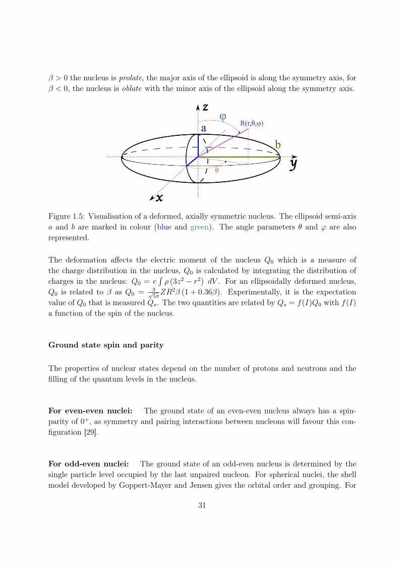
β > 0 the nucleus is prolate, the major axis of the ellipsoid is along the symmetry axis, forβ < 0, the nucleus is oblate with the minor axis of the ellipsoid along the symmetry axis.

Figure 1.5: Visualisation of a deformed, axially symmetric nucleus. The ellipsoid semi-axisa and b are marked in colour (blue and green). The angle parameters θ and ϕ are alsorepresented.

The deformation affects the electric moment of the nucleus Q0 which is a measure ofthe charge distribution in the nucleus, Q0 is calculated by integrating the distribution ofcharges in the nucleus: Q0 = e

ρ (3z2 − r2) dV . For an ellipsoidally deformed nucleus,Q0 is related to β as Q0 = 3√

5πZR2β (1 + 0.36β). Experimentally, it is the expectation

value of Q0 that is measured Qs. The two quantities are related by Qs = f(I)Q0 with f(I)

a function of the spin of the nucleus.

Ground state spin and parity

The properties of nuclear states depend on the number of protons and neutrons and thefilling of the quantum levels in the nucleus.

For even-even nuclei: The ground state of an even-even nucleus always has a spin-parity of 0+, as symmetry and pairing interactions between nucleons will favour this con-figuration [29].

For odd-even nuclei: The ground state of an odd-even nucleus is determined by thesingle particle level occupied by the last unpaired nucleon. For spherical nuclei, the shellmodel developed by Goppert-Mayer and Jensen gives the orbital order and grouping. For

31

deformed nuclei, the symmetry breaking lifts the energy degeneracy in the orbitals ac-cording to Ω, the projection of the spin J on the symmetry axis. This energy splittingleads to a reorganisation of shell levels with deformation and a change in energy gaps. Or-bitals of lower Ω are more bound for prolate nuclei – respectively, orbitals of high Ω havelower energy for oblate nuclei. This degeneracy lifting has been introduced by S.G. Nilssonand explains the stability, ground state and low lying excitation properties of deformednuclei [30]. Nilsson proposed to classify the orbitals in a deformed nucleus according tothe numbers Ω[NnzΛ] with N the main quantum number of the spherical shell (whichdetermines the parity), nz the number of excitation quanta on the symmetry axis and Λ

the projection of the angular momentum on the symmetry axis. Figure 1.6 shows theNilsson-orbitals calculated with a wood-saxon potential for SHE.

Figure 1.6: Nilsson orbitals for protons 82 ≤ Z ≤ 114 (left) and neutrons N ≥ 126 (right)as a function of the deformation (parametrized by ε). There are gaps at finite deformationthat stabilise the deformed nuclei. The position of the gaps and orbitals relevant for 254Noat Z = 102 and N = 152 are marked. (From [31])

32

1.2.2 Excited states in the nuclei

Rotational excitation

Deformed nuclei gain an extra degree of freedom and can rotate, the axis of rotation beingdifferent from the symmetry axis. On figure 1.5 or 1.7 the rotation axis would be z.

Figure 1.7: Schematic drawing of a deformed rotating nucleus. The nucleus rotates alongthe z axis, perpendicular to the symmetry axis (y). The total spin of the nucleus isI = R + J with R the rotation vector and J the intrinsic excitation spin.

The energy associated with the rotation is Erot =R2

2J with R the global rotation vector(similar to a classical body rotation) and J the moment of inertia of the nucleus. For arigid-body rotation, the moment of inertia is derived from the classical value, and for asphere is Jsphere = 2/5 M R2. For an axially deformed nucleus, the moment of inertiaalong the Z axis would be :

J = 2/5 M R2 (1 + β/3) (2/MeV) (1.6)

The moment of inertia of the nucleus is generally reduced with respect to the rigid-bodyvalues given above by the super-fluidity of the nuclear matter. The effective moment ofinertia of a nucleus is J = kJrigid with k ≈ 0.4 − 0.5 [32]. Moreover, J is not constantover the all range of excitation and spin of the nucleus: particle alignment, orbital crossingor change in deformation will modify the moment of inertia. That is why we define spin

33

dependent kinematic J (1) and dynamic J (2) moment of inertias:

J (1) = I

dE(I)dI

−1

J (2) =

d2E(I)dI2

−1 (1.7)

Because of the necessary symmetry of the nuclear wave function, for even-even nucleus onlyeven I values are allowed. Therefore the sequence of energy levels follows E(I) = I(I+1)

2Jwith I = 0, 2, 4, 6, ... This sequence of energy is a signature of rotational motion. Therotational states with the lowest energy at a given spin is called the yrast line.

Intrinsic excitations

Rotation can be built on top of the ground-state and also on top of excited states. Suchexcitations occur when one or more nucleons are excited to higher single particle levelswithin a shell (or even across a shell gap). These excitations may change the nuclei shape,spin and parity.

K quantum number

The global spin I of the nucleus has two components: the first is the global rotationalangular momentum R, along the rotational axis, the second is the spin of the intrinsicexcitation in the nucleus J ; I = R + J . One notes that, by definition and for an axiallydeformed nucleus, the rotation axis is different (often perpendicular) than the axis ofsymmetry. The projection of the total spin on the symmetry axis is noted K and is a goodquantum number for axially deformed nuclei, as strict selection rules exist for transitions.For an even-even nucleus rotating along an axis perpendicular to the symmetry axis withoutintrinsic excitation K = 0.

K isomers

When K is a conserved quantum number, transitions in the nucleus between states ofdifferent K will be disfavoured. One can visualise the transition as a potential energy withmultiple minima at different values of K. The difference in K between the two minimaimplies a small probability of electromagnetic transition. Hence, the high K states havea long life-time and constitute isomers. The trans-uranium elements display such longlived high K states [33]. Figure 1.6 shows the Nilsson orbitals and highlights the gaps for

34

254No: the orbitals at the Fermi level have a large projection of angular momentum on thesymmetry axis, leading to the formation of high-K states and isomers.

1.2.3 Decay modes

Gamma decay

The decay of an excited nucleus by electromagnetic transition is associated with the emis-sion of a photon (electro-magnetic radiation). This process does not change the mass orcharge of the emitting nucleus; however it reduces its excitation energy and the spin ischanged.

The angular momentum carried by the photon is determined by its multipolarity L. Therelation between the initial and final states spin Ii and If is L = Ii + If , or :

|Ii − If | ≤ L ≤ Ii + If

Furthermore, the parity change ∆π = πi · πf is equal to +1 or −1. The transition is calledelectric if ∆π = (−1)L and magnetic is ∆π = (−1)L+1 ; the table 1.1 summarises thedifferent transitions and their characteristics. Between two levels, the favoured transitionis the one with the lowest multipolarity.

Transition J ∆π

E1 1 -1M1 1 1E2 2 1M2 2 -1E3 3 -1M3 3 1

Table 1.1: Characteristics of electro-magnetic transitions (angular momentum carried andparity change), according to their names.

The selection rules in the transition come from the underlying quantum process: the re-duced transition probability for a σL transition (with σ the type of transition, electric ormagnetic and L the angular momentum carried by the γ-ray) is B(σL) = 1

2Ii|If |M(σL)|Ii|2

with M(σL) the matrix element for the transition. Within a rotational band, M1 and E2

35

transition probabilities are:

B(M1) =3

4π(gK − gR)2K2|IiK10|IfK|2 µ2

N (1.8)

B(E2) =5

16πQ2

0K2|IiK20|IfK|2 (eb)2 (1.9)

Here gR is the collective magnetic moment of the nucleus – independent on the intrinsicexcitation, gK the configuration magnetic moment which depends on the orbitals occupiedby the nucleons, and Q0 the quadrupole moment of the nucleus. The transition probabilitiesare strongly dependent on the configurations of the initial and final levels. Transitionsbetween two I = 0 states are not possible with γ emission, as a photon must carry angularmomentum, but internal conversion is possible for 0 → 0 transitions.

Internal conversion

Internal conversion manifests itself by the emission of an electron. The process is a caseof electro-magnetic transition, even if it is not associated with the emission of a photon.Internal conversion happens when the electro-magnetic transition energy is transmittedto an electron of the atom which is removed from the electronic cloud and gains kineticenergy. The process is in competition with γ emission, except for 0 → 0 transitions. Theinternal conversion process is favoured when: Z is large, the γ transition energy is smalland the electron wave function has a higher probability to be inside the nucleus (it is thecase for K electron shells). The multipolarity of the γ transition and the wave function ofthe electron also play a role in the conversion process. When an electron of binding energyWB is ejected by internal conversion, the energy of the electron is Ee− = Eγ − WB.

The ratio of the number of internal conversion electrons emitted over the number of γ-raysemitted is α = Ne

Nγand is called the internal conversion coefficient. It is established that

α ∝ Z3

Eγ. The internal conversion coefficients are tabulated or can be calculated [34]. For

the ground state bands in 254No, the conversion coefficients for E2 transition can be aslarge as 1545 at the lowest energy (44 keV). Table 1.2 gives the conversion coefficients forthe main known 254No transitions.

Following an internal conversion, the hole in the electronic shell is filled by electrons fromhigher shells in the electronic cloud. This process is accompanied by X-rays emission andejection of low-energy electrons (called Auger electrons), leading to multiple ionized atoms.The probability of emitting a X-ray is determined by the fluorescence yield ω which differsdepending on the electronic shells. For 254No, the ωK ≈ 1.

36

Eγ (keV) α

44 1545102 28.8159 4214 1.2267 0.54318 0.3366 0.2412 0.14456 0.11498 0.09536 0.07570 0.06

Table 1.2: Internal conversion coefficients for known 254No yrast E2 transitions. The α

coefficient decreases with Eγ.

β decay, Electron capture

β decay is the process in which the nucleus changes its charge by 1 unit; this is theprimary process in which a nucleus decays along an isobaric chain to a more stable element.The weak interaction is responsible for the reaction n → p + e− + νe for β− decay, orp → n + e+ + νe for β+ decay. The transition from ZA to Z-1A can also occur via electron

capture, a process during which a proton is converted into a neutron via the capture of anelectron from the atomic electron cloud : p + e− → n + νe [35, 36].

Alpha decay

Heavy elements (Z 50) can decay by emitting an α particle, i.e. a 4He nucleus.

The process of emitting an α particle from the nucleus is characterised by the Q-valueQ = M (A, Z)−M (A − 4, Z − 2)−M4He. The α particle energy can be approximated as:Kα ≈ A−4

AQ. For elements with A ≈ 250, Kα 95% of Q. Furthermore, the problem of

α decay can be treated, in a very simplistic approximation, as a barrier penetration withthe α particle escaping across a potential barrier. The transmission is ∝ e−2∆

√2Mα|V −Kα|/

with ∆ the barrier width. In fact, in addition to the nuclear potential well from which theα particle has to escape, there is a Coulomb and a centrifugal barrier. The alpha decayproblem, when solved, leads a relation between Q and the half-life of the nucleus T1/2 = ln 2

λα

37

with T1/2 ∝ Z√Q

. The combination of the Eα and T1/2 can be used to identify the parentnucleus – See figure 1.8 and reference [37,38].

Figure 1.8: Plot of log (half life) vs. α energy for even-even heavy nuclei – from [37].

Spontaneous fission

Spontaneous fission is a decay process in which the nucleus breaks up in two fragments.One has to separate spontaneous fission from induced fission and fission during a reactionprocess when the excitation energy causes the nucleus to fission. Spontaneous fission ischaracterised by the fissility x which is greater than 1 for elements with Z2/A 47.

38

Chapter 2

Synthesis of Super Heavy Elements

2.1 Fusion Evaporation Reactions

V&SHE are not found in nature – yet [39] – and must be produced in the laboratory.Moreover their limited stability makes them short lived. Therefore, one needs to producethem just beforehand and on location for study. Production of such elements is done eitherby deep inelastic reaction [40] or by a type of reaction called “fusion-evaporation” whichis, as the name suggest, a multi-step process. Fusion-Evaporation is a reaction where aprojectile nucleus a collides with a target nucleus A to form a compound nucleus (CN)C that will evaporate light particles b to produce the nucleus of interest B, following theequation :

a + A → C → b + B → B + γ

As the equation suggests, fusion-evaporation can be described in different steps [32]– seealso fig. 2.1 :

• Contact and capture between projectile and target

• Formation of the Compound Nucleus (fusion)

• Evaporation of particles to form the nucleus of interest.

• Emission of γ-rays in the decay to the ground state.

39

2.1.1 Capture

The first step of fusion-evaporation is the capture: the two nuclei a and A have to touch

in order to form the compound nucleus – figure 2.1. In addition to obvious geometricconsiderations to this phase of the reaction, there are conditions in terms of energy andangular momentum that need to be met to get capture between the two nuclei. There isa barrier that must be overcome: mainly from the Coulomb repulsion between the twocharged nuclei, plus a kinetic component: at low angular momentum , the phase spaceis small and makes it harder for the two nuclei to be in contact, whereas for very largeangular momentum the corresponding large impact parameter disfavours the contact. Thecontact phase is characterised by a probability P a,A

contact(Ea, ) where Ea is the kinetic energyof the projectile and is the angular momentum in the system.

The characteristic values of importance in the contact phase are :

Size of the nuclei With the radius of a nucleus given by R = r0A1/3 (r0 = 1.2 fm), the

distance between the two centres at contact is bcontact = Ra +RA +dinteraction (Ra andRA are the radii of the nuclei a and A), with dinteraction ≈ 2 − 3 fm the distance ofinteraction of the two nuclei. The impact parameter must therefore be smaller thanthis value, otherwise the nuclei can not touch.

Angular Momentum The transferred angular momentum in the reaction is given by

( + 1) = 1

µ v b, where is the angular momentum, µ is the reduced mass ofthe system (µ = mamA

ma+mA, ma and mA are the masses of the nuclei), v the speed of the

projectile (in the centre of mass frame) and b the impact parameter.

Coulomb barrier The Coulomb barrier is proportional to ZaZA

A1/3

a +A1/3

A

( Za, Aa and ZA, AA

are the charge and mass number of the nuclei) ; the energy in the centre of massmust be above this value for the two nuclei a and A to get in contact.

R. Bass described the fusion process in a classical liquid drop potential model with nodeformation and showed that the interaction (contact) cross-section can be expressed interms of a one-dimensional barrier [41, 42], with σR = πR2

int

1 − V (Rint)E

, with Rint =

Ra + RA + dinteraction and V (Rint) = 1.44 MeV ZaZA

Rint− b RaRA

Ra+RA(b ≈ 1 MeV). The potential

V (R) reflects the competition between Coulomb repulsion (∝ ZaZA/R) and the surfacetension energy (∝ RaRA/(Ra + RA)).

40

Figure 2.1: Schematic view of the fusion-evaporation reactions process. The projectilea impacts the target nucleus A with the impact parameter b. The pre-fusion system ischaracterised by the interaction distance dinteraction. At each step of the process, the systemcan fission, before forming the compound nucleus, or evolving to form the CN C∗, whichwill evaporate neutrons and γ-rays to loose excitation energy and form the evaporationresidue B.

41

2.1.2 Compound Nucleus: Fusion and Formation

The second step in a fusion-evaporation reaction is the formation of the CN; i.e. thepassage from 2 nuclei in contact into one excited nucleus at thermal equilibrium (C).The CN formation implies a change of the shape (see figure 2.1) often characterised by abarrier the system needs to pass in order to make the transition. The transition to the CNmust happen on a time scale of the order of the time needed for the bombarding particlesto travel across the target nucleus (i.e. approximately 10−21s) [43]. The reaction energyis shared among all the CN nucleons, leading to a nucleus with an excitation energy E

equal to the total energy in the system plus the Q-value (negative) to form the CN. TheCN exists over a time scale of the order of 10−19 to 10−16s. The formation of the CN willdepend on the beam energy E, the angular momentum and the entrance channel. Theprobability to form the compound nucleus is given by PA+a→C

CN (E, ) [44]. If the formationof the CN fails, the pre-compound system a + A splits into target-like and projectile-likefragments; this process is called quasi-fission – see figure 2.1.

Deformed nuclei barrier

The barrier described above considers only spherical nuclei. For a deformed nucleus, thebarrier, which depends on the interaction distance, cannot be expressed as simply fordeformed nuclei, it depends on the relative orientation η of the nuclei: Rint(η) = Ra +

RA + dinteraction(η). As the orientation η is not controlled, there is a distribution of barriersspread over all the possible η configurations.

Coupled channel

To the simple geometrical approach, one must add the refinement of quantum mechanics.During the reaction process, the nuclei can be excited to their internal excited levels [45].The coupling between the internal excitation configurations will enhance or reduce thefusion probability depending on the configuration, possible shape changes in excited states,... This modifies the barrier distribution as a function of reaction energy.

For the 48Ca on 208Pb reaction, coupled channels calculations are necessary to reproducethe experimental capture cross-sections below and around the fusion barrier. Withoutcoupling, there is only one barrier. Coupling to 1-phonon excitations in the nuclei makesadditional barriers appear and higher-order coupling lowers the secondary barriers, makingthem reachable in experiment. Figure 2.2 shows an example of barrier distributions for

42

254No. Therefore coupling creates a secondary maximum in partial fusion transmission atlower angular momentum. Figure 2.3 shows calculations from [46].

Figure 2.2: Calculation of the barrier distribution as a function of centre of mass energy for254No in the reaction 208Pb(48Ca,2n)254No with no coupling (red), excitation of one (black)and excitation of two (blue) phonons in the target and projectile nuclei. The blue arrowshows the centre of mass energy in our experiment at EBeam = 219 MeV and the red arrowat EBeam = 223 MeV, which is below the second barrier with only one phonon couplingbut above it when coupling two phonons. From [46].

2.1.3 Evaporation

The last step of the fusion-evaporation reaction is the evaporation by the CN of lightparticles (protons, neutrons, α particles) of emission of γ-rays to form evaporation residues.When formed, the CN has an excitation energy E = Ecm + Q, where Ecm is the totalenergy available in the centre-of-mass frame (Ecm ∼ K + AA + Aa, with K the kineticenergy of the projectile in the centre-of-mass frame) and Q the Q-value for forming theCN (Q = BECN − (BEa + BEA)), Q being negative for typical reactions in the formationof heavy nuclei.

43

Figure 2.3: Partial transmission coefficient for the fusion of 48Ca with 208Pb at projectileenergy of 219 MeV (black) and 223 MeV(red) calculated without (left) and with (right)coupled channels. The channel coupling creates a secondary peak from the higher barrier,following Lmax ∝

√ECN − B (with ECN the excitation energy of the compound nucleus

and B the fusion barrier height). From [46].

44

The evaporation process happens on a long time scale (as long as 10−15s, compared to thetypical orbit time of a nucleon in the nucleus: 10−21 s). The process is statistical and theevaporation channels are independent. Evaporation of neutrons is strongly favoured sinceit is not hindered by the Coulomb barrier. Protons and α particles evaporation is usuallynot observed from heavy CN, although it is theoretically possible. Fission will competewith particle and γ emission.

Neutrons (or more generally particle) evaporation reduces the CN excitation energy by theseparation energy and the kinetic energy of the evaporated particle. However, evaporationdoes not affect the angular momentum very much. Particles will be evaporated as longas E is above the particle separation energy. When E < Sparticle for any particle, theCN will emit statistical γ-rays, mainly of E1 multipolarity, carrying energy and very lit-tle angular momentum, bringing the nucleus closer to yrast and other excited rotationalbands constituting the normal γ-decay path – see figure 2.1. The evaporation to a givenevaporation residue (ER) is characterised by the probability PC

ER(E, ).

Decay widths

The decay of the compound nucleus by emission of neutrons and other particles, γ-raysor by fissionning is governed by the associated decay widths [47]. According to Fermi’sgolden rule, the width for a decay is Γ = 2π

|M |2ρ – where M is the transition matrix

element and ρ the phase space factor, measuring the density of final states. In terms ofglobal quantities, the width can be expressed as the ratio of the number of available finalstates N over the level density at the initial state ρ: Γ = N

2πρ. The number of available

final states is obtained by integrating the level density of the final states over the availableenergy range.

Level Density The level density is a key parameter for the calculation of decay widths.It is not an easy quantity to measure at intermediate energies and is parametrized fromtheory [48]. A classical parametrization is [8, 48–51]:

ρ (E∗, J) =2J + 1

24√

2a1/4 (E∗ − Erot(J) − ∆)5/4σ3

exp

2

a(E∗ − Erot(J) − ∆) − (J + 1/2)2

2σ2

MeV−1

(2.1)Here a is the level density parameter, of the order of A/8, Erot(J) the rotational energy= J(J+1)

2Jg.s., ∆ is the pairing gap, of the order of 24/

(A) for even-even nuclei, equal to 0 in

other cases and σ is the spin cut-off parameter: σ =JrigidT

where Jrigid is the rigid body

moment of inertia and T the temperature of the system.

45

More complex factors affect the level density: There is an enhancement of the level densityby collective excitations (ρenhanced(E

∗, I) = Kcollective(E∗, I)ρ(E∗, I) [52, 53]). In addition,

damping of shell effects with excitation energy [8, 48], needs to be taken into account,by using adamped = a[1 + δ 1−exp(−γDE∗)

E∗] with δ the shell correction and γD the damping

parameter [50]. The way to implement such damping in the calculation is currently underdiscussion, see appendix D.

Fission Potential Even if fission eventually leads to a gain in energy (the binding energyof the two fragments is higher than the one of the initial nucleus) during the process, thesystem has to overcome the fission barrier, noted Bf .

An easy way to represent the fission process is having the system moving along the energypotential V as a function of deformation β. During the fission, the nucleus undergoes atransition from inside the potential well, around βg.s., to a higher deformation β. In order toget over the saddle at βsaddle (the deformation “threshold” over which the nucleus becomesunbound and fissions) the system must go over Bf = Esaddle − Eg.s. – see figure 2.4. Thesaddle energy can be parametrized by Esaddle = Bf (0) +

2I(I+1)2Jsaddle

, with Bf (0) the height ofthe fission barrier at spin 0, and Jsaddle the moment of inertia of the saddle, assuming arotor behaviour, with Jsaddle linked to the saddle deformation βsaddle.

The quantum nature of the system implies that a tunnelling of the wave function throughthe potential is possible when E∗ < Esaddle. Therefore, the transition from a non fissionningnucleus to fission with increasing E is not sharp but smooth; depending on how strongthe tunnelling is and the competition with other decay modes (given by Γfission/Γtotal).

The fission barrier Bf is a framework of calculation used to model the fission process andis not directly observable. However, the fission barrier is computed and is used in allcalculations. Furthermore, the quantity Bf is linked to very experimental observables likethe maximum excitation energy one can put in the nucleus before it fissions, spontaneousfission half-lives, fission probability in reactions, etc. Hence it is a parameter that can bededuced from experimental data.

Fission decay width For the fission decay, the number of final states is given by in-tegrating the level density above the saddle point energy up to the excitation energy. Inpractice, due to the barrier penetration in the fission process, the integration goes from 0to E∗ with a tunnelling factor, characterised by the energy ω. The tunnelling parameterω is linked to the curvature of the potential (supposed parabolic) around the saddle andusually taken to be ≈ 1 MeV. The fission width grows rapidly above the threshold energy

46

Figure 2.4: Schematic potential energy for fission against the deformation parameter (β).The ground state, located at a finite deformation and the saddle point at higher deformationdefine the fission barrier Bf . A schematic view of the shape of the nucleus is representedabove the potential.

47

Bf and can be expressed as [54–56]:

Γfission =1

2πρg.s.(E∗)

E∗

0

ρsaddle(E∗ − ε)

1 + exp

−2π(ε−Bf )

ω

dε MeV (2.2)

In the formula, the denominator is the transmission through the barrier (tunnelling).

Neutron decay width For the neutron decay, Weisskopf calculates the widths in theframe of the equilibrium reaction AZ n + A-1Z, following the transition state theory.One has to introduce the cross-section of the reverse reaction (neutron capture) in thecalculation. The integration is done over the excitation energy above the neutron separationenergy Sn and for the level density of the A-1Z nucleus. A pre-factor appears due to thekinematic degrees of freedom of the neutron and the spin degeneracy (g). There is notunnelling for neutron emission. This leads to [8]:

Γneutron =gm

π22

1

ρA(E∗)

E∗−Sn

0

ε σinverse (ε) ρA−1 (E∗ − Sn − ε) dε MeV (2.3)

The Weisskopf approach does not depend on the spin of the initial and final state. Toaccount for angular momentum and barrier penetration, the Hauser-Feshbach formalism isbetter suited and considers the angular momentum carried by the emitted neutron [8,57].

γ decay width For γ decay, the width depends on the transition multipolarity and thestrength function specific to a nucleus (in particular the deformation).

For an E1 multipolarity transition, the strength function has a Lorentzian form, followingthe Giant Dipole Resonance energy and width: fE1(Eγ) = C EγΓGDR

(E2γ−E2

GDR)2

+Γ2

GDRE2

γ

, with C

a constant factor and ΓGDR and EGDR are the Giant Dipole Resonance width and energy.The strength function typically has a value of a few 10−6 MeV−1. For axially deformednuclei, the strength function depends on β, the quadrupole deformation parameter and hasseveral maxima, compared to only one for spherical nuclei.

The γ decay width also depends on the γ energy to the power of 2L + 1, with L the γ

multipolarity. There is no threshold energy to emit a γ-ray. An E1 γ can carry one unitof spin and one has to sum over the different final possible spins.

This leads to an E1 γ decay width of [58,59] :

ΓE1γ =

1

ρ(E, I)

J=I+1

J=I−1

E

0

ε3fE1(ε)ρ(E − ε)dε MeV (2.4)

48

Decay probability The decay probability for a given decay channel is given, in term ofwidth as Pdecay =

Γdecay

Γtotal, with Γtotal the sum of all decay channel widths [60]. In the case

of fusion-evaporation, the probability of fission is Pfission = Γfission

Γfission+Γneutron+Γγ.

The probability to form an evaporation residue B by emitting two neutrons from thecompound nucleus C∗ will be given by: PC∗→B

ER = ΓC∗

n

ΓC∗

total

× ΓC∗−n

n

ΓC∗−n

total

.

2.1.4 Evaporation residue formation

The total probability of formation of an ER at a given excitation energy from the a + A

reaction is therefore characterised by the cross section [50] :

σER(E) =π

2

2µE

∞

L=0

(2L + 1) · P a,Acontact(Ea, L) · PA+a→C

CN (E,L) · PC

ER(E, L) (2.5)

µ is the reduced mass, as introduced in 2.1.1.

The fission barrier affects the term: PC

ER(E, L). Theoretical calculations, although theymanage to give rather good predictions for the cross section σER, fail to agree for thedifferent terms and steps of the process. This is a big limitation of the calculation sincethe internal steps of calculation rely on complex process and hypotheses that cannot beindividually verified experimentally and that are not unique in their modelisation.

2.2 Hot and Cold Fusion

Fusion-evaporation can be hot or cold, depending on the excitation energy of the CN. Thechoice of projectile-target combination determine which of the two regime happens.

2.2.1 Cold fusion

Cold fusion relies on magic or nearly-magic projectile and target (like 48Ca and 208Pb or209Bi). As a consequence, the reaction Q-value is very negative (the magicity gives a largebinding energy and Q = EB(CN) − (EB(a) + EB(A)) is therefore large and negative) andthe CN excitation energy is low (around 10–20 MeV). The CN evaporates only one or twoparticles (predominantly neutrons).

49

In cold fusion, the capture is disfavoured by the high Z1Z2 term in the potential energy; butthe low excitation energy of the compound nucleus favour the survival of the evaporationresidues.

2.2.2 Hot fusion

For hot fusion, heavier targets and more asymmetric projectile / target combinations areused (for example 244Cm on 12C to produce 254No). The CN excitation energy is usuallyaround 50 MeV and 4 or 5 neutrons are evaporated.

In hot fusion, the lower Z1Z2 favours the contact between projectile and target nuclei; butthe higher compound nucleus excitation energy reduces the survival probability of the ERs.

2.2.3 The case of 254No

254No can be produced via hot and cold fusion, the different beam-target combination givedifferent Q-values and production cross section, as shown in table 2.1.

Reaction Q-value (MeV) CN E∗ at max. σ (MeV) Max. σ (µb)238U(22Ne,6n) [61] -93.9 57 15±7 × 10−3

208Pb(48Ca,2n) [61, 62] -166.8 21 2

Table 2.1: Table of Q-values and production cross section for hot and cold fusion toproduce 254No. The compound nucleus excitation energy at the maximum of cross sectionis indicated. The difference between the hot and cold reactions are clearly visible in termsof the Q-values, E∗ and σ.

Independently of the type of fusion-evaporation reaction, the production cross section in theregion of V&SHE falls exponentially with the atomic number Z of the produced element.Figure 2.5 shows the evolution of production of SHE cross section with neutron numberfor hot or cold fusion.

50

Figure 2.5: Plot of cross section for cold and hot fusion reactions, as a function of thecompound nucleus neutron number (from [63]). The plot shows an exponential decreasein cross-section for both hot and cold fusion up to N=170, above which values there is anincrease for 48Ca induced reactions. This increase corresponds to higher Bf predicted inmacroscopic-microscopic models (see chapter 3): Calculation predict Bf ≈ 7 − 8 MeV forN 170 while the fission barrier is lower around 6−7 MeV for N between 150 and 170 [1].

51

2.3 The importance of Fission

In fusion evaporation, fission is in competition with every steps of the ER formation process:

• The a + A system can fission during the formation of the CN (quasi-fission).

• The excited CN C can fission.

• The excited ER C − xn can fission.

For heavy elements, fission will be in strong competition with neutron evaporation andother decay channels (because of the strong Coulomb repulsion in the large system). Hence,the production of the ER will be weak and have very small cross sections, of the order ofµbarn of less. In fact, the evaporation residues cross-section is about 4 orders of magnitudesmaller than the capture; as shown in figure 2.6.

Figure 2.6: Capture (black) and ER (red) cross-section for 254No in the 48Ca + 208Pbreaction. From [9].

2.3.1 The fission process

As much as the fusion-evaporation process is complex and multi-step, the same is truefor fission. During fission, the nucleus goes from one continuous body to two separatedfragments: A → F1 + F2 – fission to more than two fragments is possible, but significantly

52

less probable. Emission of light particles (neutrons, protons, ...) and γ-rays can happenas the fragments may be formed in an excited state. The process implies a deformation ofthe nucleus from a null or limited value to an infinite one (see figure 2.4). [64–66]

A. Sierk describes the barrier in the frame of a macroscopic rotating nucleus model [67],where nuclear energy, surface energy, Coulomb energy and shape energy compete, leadingto a macroscopic fission barrier value and its spin dependence. Deviation from the Sierkbarrier indicates strong shell effects that stabilise the nucleus [68,69].

2.3.2 Bf dependence on I

When the nucleus picks up angular momentum, the potential energy previously described(figure 2.4) is modified. In particular, for deformed nuclei, the rotational energy will changethe position of the well (mostly its energy, but a change in β can happen). Similarly, thesaddle energy Esaddle will change, but with a trend different from the change of the wellminimum (βsaddle can also change) – see figure 2.7. In terms of moment of inertia, thefission barrier and its spin dependence can be expressed as :

Bf (I) = Bf (0) − 2I(I + 1)

2

1

Jg.s.

− 1

Jsaddle

(2.6)

with Jg.s. and Jsaddle the moment of inertia of the ground state and the saddle point andBf (0) = Esaddle − Eg.s. the fission barrier height at spin 0.

The spin dependence of Bf is a good way to probe the spin dependence of shell effects thatstabilise the ground state, since Bf (I) can also be expressed as Bf (I) = Esaddle(I)−Eg.s.(I),with both quantities Esaddle(I) and Eg.s.(I) (the energy of the ground state band) dependingon shell effects.

2.3.3 Probing the fission barrier

For nuclei which can be populated by transfer reaction, probing the fission barrier isstraightforward: one observes the fission as E increases [6, 7], which is a way to probePfission = Γfission/Γtotal. For VHE and SHE such as 254No, it is not possible since there isno suitable target-projectile combination to excite the nucleus by transfer reaction [70].However, the γ and fission decay are in competition, and one can observe this competitionvia Pγ = Γγ/Γtotal which provides information on Bf . In cases when Sn is larger than Bf

by at least ≈ 1 MeV, Pγ ≈ Γγ/ (Γγ + Γfission). The fission width rapidly dominates γ-decay

53

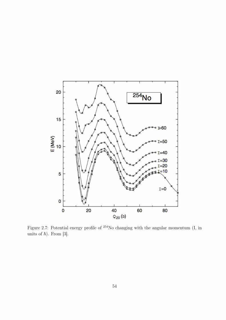
Figure 2.7: Potential energy profile of 254No changing with the angular momentum (I, inunits of ). From [3].

54

as E∗ increases. This causes a rapid drop of Pγ [27, 51, 71–74] which provides a sensitiveprobe of Esaddle, as will be discussed in the next chapter.

55

56

Chapter 3

Theoretical calculations

3.1 Theoretical predictions of the fission barrier height

and spin dependence

As mentioned earlier in section 2.1.3, the fission barrier, or the saddle energy, is a theoreticalconstruct, relevant because it is calculated in all models and for all processes related tofission. There are several ways to calculate the position of the saddle Esaddle and the spindependence characterised by Jsaddle.

Liquid drop barrier

The barrier can be calculated in a purely liquid-drop framework, using the model developedby A. Sierk [67]. These calculations do not include any shell effects and the height of thefission barrier for 254No is very small (less than an MeV). The model also predicts a momentof inertia for the saddle, but it is important to notice that it fails to reproduce the ground-state rotational moment of inertia, as pairing is not included.

Macroscopic-microscopic calculation

A more complete way to calculate the fission barrier is to rely on a so called macroscopic-

microscopic calculation, which relies first on a liquid drop model in a 5-dimensions en-vironment to account for the high-order deformations, plus shell effects introduced via

57

single-particle energies [1, 2]. Such calculations predict larger fission barrier thanks to theshell effects. However, they do not calculate properties at high spin and hence do not givea moment of inertia for the saddle.

Hartree-Fock-Bogoliubov calculation

In the more complex theoretical frame, self-consistent calculations can be performed, forexample within the framework of the Hartree-Fock-Bogoliubov method [3–5]. This methodcomputes energies and deformations and can predict both the height of the barrier and itsspin dependence.

Table 3.1 gives a summary of all the calculated height and saddle moment of inertia forthe fission barrier in 254No. The scaled SD moment of inertia is calculated by scalingthe super-deformed band moment of inertia in 194Hg to the 254No mass and saddle defor-mation βSaddle = 0.5; this method takes into account the effect of pairing in the saddle,independently of any model.

Model Bf (I = 0) (MeV) Jsaddle (2/MeV) Jg.s (2/MeV)Sierk (a) 0.9 152.0 135Macro-Micro with folded Yukawapotential [1]

6.76

Macro-Micro with Wood-Saxonpotential [2]

6.76

HFB with Gogny D1S force [3] 8.66 140HFB with Gogny D1S force [75] 6 – 7HFB with Sly4 force [5] 9.6HFB with SkM* force [4] 8.6Scaled SD 146Rigid Body 181 160Experimental value 75.0

Table 3.1: Table summarising the theoretical predictions for the 254No saddle energy. Theg.s. band (yrast) moment of inertia is reminded. (a) The Sierk model does not predict acorrect ground state moment of inertia.

58

3.2 Entry distribution calculation

We will use computer codes to simulate the entry distribution in the 208Pb(48Ca, 2n)254Noreaction. The objective is to investigate the evolution of the entry distribution with beamenergy, the effect of the fission barrier on the distribution and have a point of comparisonwith experimental measurements. Different codes have been tested: analytic calculationsand statistical simulations.

3.2.1 Analytic width calculations

Using the simple width formulas given previously (see section 2.1.3) one can calculateΓneutron,Γfission and Γγ and extract Pγ (I, E∗). In particular, one can look at the E∗ whenPγ falls below 50%: E1/2(I). These calculations can be done with Bf(I) arbitrarily set toany value. One notes however that this calculations do not take the population of (I, E∗)

states in 254No in the reaction into account. Figure 3.1 shows the decay widths and thedecay probability as function of excitation energy in 254No.

3.2.2 evapOR calculation

The code evapOR [76] is an extension of the PACE2 code, which allows multi-particle evap-oration in a Monte-Carlo framework. It takes as input the target and projectile informationand the beam energy. It has been modified [77] to output an entry distribution and so thatit is possible to vary the values of Bf . However, although evapOR manages to reproducefairly well previous experimental measurements like the entry distribution in 192Hg [78], theresults calculated for 254No are hard to interpret, as no evidence of fission barrier effectsare seen in the calculated entry distribution and no elements were available to validatethe evapOR results (for example, evapOR fails to reproduce production cross-sections for254No). Figure 3.2 shows tentative calculation with evapOR with increasing beam energybut no visible effect of fission, contrary to the expected behaviour. It was therefore decidednot to trust those calculations and attempts to use evapOR were dropped.

3.2.3 KEWPIE2

The code KEWPIE2 [8, 79, 80] was written at GANIL to study the fission time in SHEsynthesis. It contains a Hauser-Fesbach component, which calculates the population and

59

Figure 3.1: Decay widths (Top) and Decay mode probability (bottom) for I = 0 cal-culated with analytic width formulas, the γ (red) and fission (blue) widths cross at E1/2

which is close to the saddle energy, represented by the blue line. The neutron evaporationwidth is in black and kicks in at Sn = 7.71 MeV. The γ probability falls below 0.5 at E1/2

which is the energy where Γfission = Γγ and is slightly (≈ 1MeV) above Bf, marked with ablue line.

60

decay of nuclei at given (I, E∗). It takes as input the projectile and target nuclei and thecompound nucleus excitation energy, the fusion probability is obtained with a proximitypotential. Moreover, the code is available and can be modified to suit our needs. It istherefore perfect for calculating entry distribution. As the code was not primarily createdto that end, modifications were made to take into account the nuclear deformation andensure a proper spin dependence of all parameters. KEWPIE2 uses mass, deformation andfission barrier data from [1].

The population of states at (I, E∗) and the decay widths are computed by the modifiedKEWPIE2 code and then processed into an entry distribution. The entry distributionis populated according to which (I, E∗) states are populated by the neutron decay from255,256No and which of those γ decay contribute to the entry distribution.

Figure 3.3 shows a calculation of the entry distribution for 254No. In particular, we lookat the energy where Γγ ≈ Γfission and Γγ ≈ Γneutron.

The KEWPIE calculations display an entry distribution spilling over Esaddle at low spin.In other words, E(Pγ=0.5) = 0.5 is above Esaddle and E(Pγ=0.5) − Esaddle decreases with spin,which is the same behaviour as suggested in the simple width calculation. The calculationsalso indicate no effect of neutron evaporation is affecting the entry distribution since theΓγ ≈ Γneutron line is largely above the saddle energy. Finally, the calculations indicate that(I, E∗) states populated by neutron decay are high enough in energy to be directly affectedby the fission barrier. Therefore, the truncation of the entry distribution by the fissionpermits Esaddle to be extracted.

Figure 3.4 shows examples of entry distribution at the two beam energies, calculated withKEWPIE2.

3.2.4 NRV calculation

We also used the NRV calculations [9] to simulate an entry distribution. Through the NRVwebsite, one can compute the cross-section, partial fusion cross section and decay width fora given nucleus as a function of I and E∗. By combining all these data, one can simulatethe fusion and decay in the 208Pb +48 Ca reaction down to the (I, E∗) states in 254No thatγ decay – hence reconstructing the entry distribution. The input is the compound nucleus(I, E∗) distribution. For consistency, we used the same distribution as the one used inKEWPIE2. This calculation method has two major drawbacks:

• It is not a fully integrated calculation but a code putting together elements from

61

Figure 3.2: Plots of the evapOR calculation with Bf (I = 0) set at 7 MeV and the CNexcitation energy increasing from 219, to 221 to 223 MeV. The yrast line is represented inblack, the purple line is the saddle energy and the red dotted line is the neutron separationenergy. One can see that the spin distribution does not change and the energy distributionis just shifted up. There is apparently no effect of the fission barrier.

Figure 3.3: Entry distribution of 254No at Ebeam = 219 MeV calculated with KEWPIE2.The yrast line is in red, the saddle line used in the calculation is the purple line and theneutron separation energy is the gray line. The energy where Pγ ≈ 0.5 is marked in orangeand the energies where Γγ ≈ Γfission and Γγ ≈ Γneutron are marked in blue (concurrent withthe orange line) and green.

62

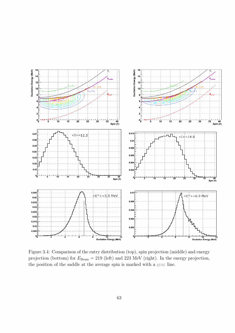
Figure 3.4: Comparison of the entry distribution (top), spin projection (middle) and energyprojection (bottom) for EBeam = 219 (left) and 223 MeV (right). In the energy projection,the position of the saddle at the average spin is marked with a gray line.

63

different sources.

• The decay procedure does not take into account pre-fission or pre-neutron γ emission(although this is probably a very low probability).

Figure 3.5 shows and entry distribution calculated using NRV. Like the distribution fromKEWPIE2, it spills over the saddle at low spin and the falling point is shifted down inrespect to ESaddle with increasing spin.

Figure 3.5: Entry distribution of 254No at 223 MeV calculated using NRV. The yrast lineis in red, the saddle energy used in the calculations in purple and the neutron separationthreshold is the gray dotted line.

With this method, we do not have control of the position and spin dependence of the saddle– or the implementation of shell effects damping, see appendix D. But we can change theprofile of the entrance channel partial fusion cross section. We can therefore verify theindependence of the final 254No entry distribution with the entrance channel, as shown onfigure 3.6: the evaporation-residue spin distribution changes somewhat with the input spindistribution, but it is clear that partial waves higher than ≈ 25 do not survive againstfission. Therefore, the maximum spin reached by the evaporation residue is not dependenton the high spins in the entrance distribution.

64

.

Figure 3.6: Profile of entrance (black) and final (green) spin distributions calculated inNRV for two different partial fusion cross section calculations; in particular, the bottom onefollows the double peaked distribution suggested by coupled-channel calculations (see 2.1.2and [46]). The final distribution of spin slightly changes with the entrance distribution, inparticular the position of the maximum. The maximum spin in the evaporation residuedistribution is not changed: Imax ≈ 25 for both entry spin distribution, because fissiondepletes the highest partial waves.

65

3.2.5 Calculations of entry distribution: results

The global characteristics of the entry distributions calculated with the two different codes,for two different beam energies corresponding to the experimental measurements, are givenon table 3.2. We see that :

• The NRV calculations give slightly lower spin and excitation energy than KEWPIE2.

• The average spin of the entry distribution increases by ≈ 3 when increasing thereaction energy in both cases. The spin distribution width increases also by 1 .

• The average excitation energy of the entry distribution increases by 0.7 to 1 MeVwhen increasing the reaction energy. The energy distribution width increases onlyslightly (by 0.1 MeV).

CodeBeamEnergy(MeV)

AverageSpin ()

Spin Width()

AverageEnergy(MeV)

EnergyWidth(MeV)

NRV219 9.8 6.1 5.2 1.2223 12.4 7.2 5.9 1.3

KEWPIE2219 11.5 5.7 5.9 1.2223 14.8 6.7 6.9 1.3

Table 3.2: Comparison of the global characteristics of the calculations results from NRVand KEWPIE2 calculations.

As the two codes use the same entrance spin and energy distribution in the CN, thedifferences in results originate from the treatment of neutrons and γ-decay, in particular,the choice of parametrization of the level density will have a huge influence (damping, spincut-off, ...). Therefore, the differences reflect the different theoretical approaches.

The two codes use the same saddle energy dependence, with a Jsaddle smaller than thetheoretical predictions: ≈ 80

2/MeV. But this can be changed in KEWPIE2 and we caninvestigate the effect of a higher or lower saddle, and different spin dependence, in orderto determine how the parameters influence the entry distribution. Figures 3.7 and 3.8show examples of entry distributions calculated with different parameters for the saddle.Calculations with changing Bf (0), all other parameters being fixed, show that an increase inBf (0) increase the average energy of the entry distribution, as one would expect. Also, thewidth of the energy distribution decreases and the average spin decreases. For Esaddle ≈ Sn,

66

the competition with neutron evaporation stops the trend of decreasing average spin – seefigure 3.9. For increasing Jsaddle, all other parameters being fixed, we see a decrease ofaverage spin and energy, and a small reduction of spin and energy widths, see figure 3.10.

Figure 3.7: Entry distribution calculated by KEWPIE2 for Bf (0) = 5 (left) and 6.5 MeV(right), with JSaddle = 80

2/MeV.

Figure 3.8: Entry distribution calculated by KEWPIE2 for Jsaddle = 117 (left) and175 /MeV2, with Bf (0) = 6.5 MeV.

Relation between E1/2 and Esaddle

In the calculations, we notice that at low spins, the entry distribution spills above the saddleenergy line. To understand why the γ-decay stays strong above ESaddle, we will consider thequantity E1/2, defined as the energy where Pγ(E

∗) = 0.5, with Pγ = Γγ/ (Γγ + Γneutron + Γfission)

(see section 2.1.3). We will define an equivalent quantity in the experimental entry distri-bution.

67

Figure 3.9: Evolution of the global characteristics of the entry distribution simulated withKEWPIE2 for different values of Bf (0). The neutron separation energy (Sn = 7.71 MeV)is marked with a blue line. Average (left) and width (right) of the spin (top) and energy(bottom) distributions.

68

Figure 3.10: Evolution of the global characteristics of the entry distribution simulated withKEWPIE2 for different values of Jsaddle. Average (left) and width (right) of the spin (top)and energy (bottom) distributions.

69

The E1/2 energy is linked to the saddle energy and the relation between the two as afunction of spin ∆(I) = E1/2(I) − Esaddle(I) can be extracted from calculations. In thelimit of Esaddle < Sn, E1/2 is found by solving Γfission = Γγ. One can consider that Γγ

grows exponentially with excitation energy, while Γfission grows with E∗−Bf , therefore, forspins where Bf is large (at low spins) Γγ is large when the excitation energy is around Bf

while the fission width is still small, and E1/2 will be higher than Esaddle. At higher spins,where Bf is smaller, Γγ is not as large at Bf and the fission and γ widths are equal at anexcitation energy closer to Bf .

Figure 3.11: Profile of ∆(I) = E1/2(I) − Esaddle(I) obtained from analytic width calcula-tions. The points are the calculated values, uncertainties come from integration steps, linesrepresent quadratic fits. The red and blue series correspond to two different parametriza-tion of the saddle: Bf (0) = 6 MeV and Jsaddle = 150

2/MeV in red and Bf (0) = 6.5 MeVand Jsaddle = 170

2/MeV in blue.

Figure 3.11 shows the profile of ∆(I): One can see that the E1/2 points are above Esaddle

at low spin and this difference decreases at higher angular momentum. Those calculationslead to ∆(I = 0) ≈ 1 MeV and falling to ∆(I ≈ 30 ) = 0.

It is very important to notice that ∆(I) is a calculated quantity that depends on the Bf (I)

used in the calculation, and also on the calculation model. In figure 3.11 we see that smallchanges in the saddle energy parametrization affects ∆ only slightly. Also, as shown infigure 3.12, each code gives a different behaviour for ∆(I). One will have to be careful ofthe self-dependence of Bf extracted from experimental data using a calculated ∆.

70

Figure 3.12: Values of E1/2 from different calculations: NRV (orange), KEWPIE2 (green)and analytic calculation (blue) compared to the Esaddle parametrization (purple line). Theyrast line is the red line. The E1/2 points are above Esaddle by as much as 2 MeV at lowspin and decrease with respect to Esaddle with increasing spin.

71

3.3 Conclusion on calculations

From the calculations, we learned:

• The average spin of the entry distribution is expected around 10 – 15 and thedistribution extends up to spin 25 .

• The average energy in the entry distribution is expected around 5 to 7 MeV with thedistribution extending up to 8 MeV.

• Increasing the beam energy from 219 to 223 MeV increases the average spin by upto 3 and the excitation energy by 1 MeV.

• With larger Bf (0), higher excitation energies in the entry distribution are obtained.With larger moment of inertia Jsaddle, the maximum spin is reduced.

• The entry distribution is clearly truncated at E1/2 which is above Esaddle at low spinand decrease with higher spins.

These calculations clearly show that the entry distribution is largely dependent on theposition of the saddle (it also slightly depends on the entrance spin distribution), and thatconfirm the possible extraction of the fission barrier from an entry distribution measure-ment.

72

Chapter 4

Experimental measurement of Fission

Barrier

4.1 Experimental setup

4.1.1 Reaction

The reaction used to produce 254No is 208Pb(48Ca,2n)254No. This reaction is well docu-mented and has been used since 1979 to produce 254No with a reasonable cross section.References [62, 81, 82] gives the excitation function for the reaction, reproduced in figure4.1. One can see the 254No can be produced with cross-section up to about 3 µbarn. Thebeam energies used in the experiment are 219 and 223 MeV – respectively 178 and 181 MeVin the Center of Mass frame. These energies are above the peak of the cross section. How-ever, the energy loss in the target will bring the beam energy down to a correspondinghigher cross section, and more importantly, as we intend to populate 254No at the highestspin possible the higher beam energy will bring more angular momentum to the system.Due to energy spread in the target, the incoming 48Ca energy varies between 218.2 and214.5 MeV (222.3 and 218.5 MeV respectively) in the laboratory frame. The correspondingmaximum excitation energy depends on the centre of mass energy and the Q value of thereaction E∗

max = Ecm + Q. Table 4.1 gives the relevant energies. The maximum excitationenergy for the 254No is between 8 and 11.0 MeV (between 11 and 13.5 for 223 MeV beam).At those energies, the cross-section are of the order of 2 µbarn for the 219 MeV beam and1 µbarn for the 223 MeV beam (cross sections at mid-target energies)– see figure 4.1.

73

Figure 4.1: Excitation function for the 208Pb(48Ca, 2n)254No reaction. The position of theBass barrier is marked by Ex [81, 82].

74

208Pb + 48Ca → 256No Q−value -153.8 MeV256No 2 neutrons separation 13.04 MeV256No neutron separation 7.05 MeV255No neutron separation 5.99 MeV208Pb + 48Ca → 2n + 254No Q−value -166.6 MeV254No neutron separation 7.71 MeV

Table 4.1: Q−values for the formation of the compound nucleus and the 254No residue.The neutron separation energies are also given. The Q−value of the full reaction is equalto QCN − S

256No2n . By definition, S

256No2n = S

256Non + S

255Non .

Reaction kinematics

The reaction kinematic characteristics are given in table 4.2. The kinematics of the reactionare of importance for the separation of the recoils after the target (in the FMA see section4.1.7) and the Doppler correction of the γ-ray energies. In addition to purely kinematicconsiderations, the beam and recoils loose energy in the target. That influences the reactionenergy and recoil speed. For 254No recoils, the stopping power in matter is not known andhas to be extrapolated from the heaviest known nuclei to the appropriate mass with thesame kinematic energy per nucleon. The recoiling 254No have an angular dispersion (halfangle) of the order of 3.8 in the laboratory frame (this has to be compared with theseparator solid angle acceptance : 8 msr or 5.6 aperture – see section 4.1.7) – taking intoaccount the kinematic dispersion from the neutron evaporation and the straggling in thetarget material.

4.1.2 Beam structure

The beam of 48Ca was delivered by the ATLAS accelerator with a charge state Q = 11+

as a 12.1 MHz (82.48 ns period) pulsed beam. The average intensity was 100 enA, varyingbetween 90 and 120 enA – giving a current of 8.2 to 10.9 pnA. Figure 4.2 shows the beamstructure visualised as time of γ-ray events. The current was held down to avoid saturatingGammasphere with fission gammas and neutrons.

75

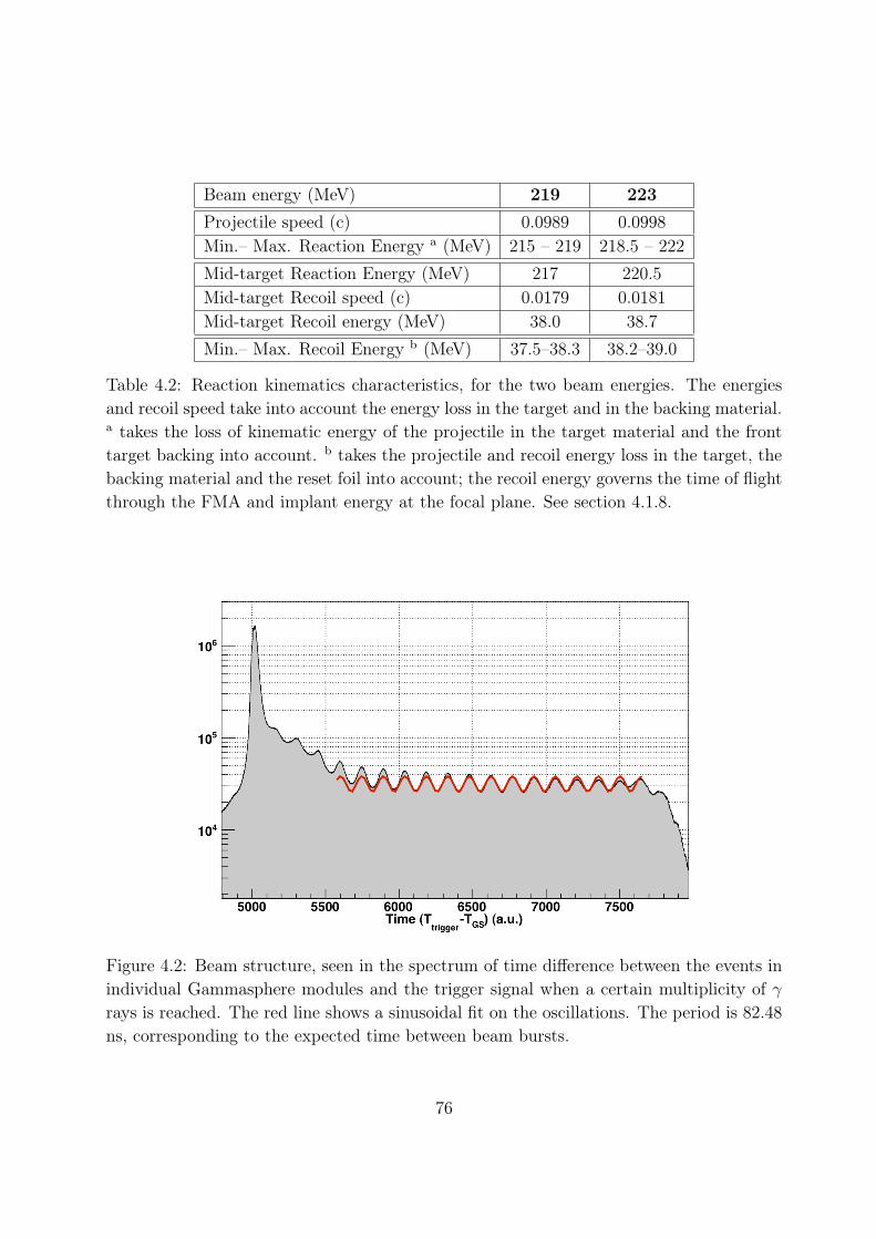
Beam energy (MeV) 219 223

Projectile speed (c) 0.0989 0.0998Min.– Max. Reaction Energy a (MeV) 215 – 219 218.5 – 222

Mid-target Reaction Energy (MeV) 217 220.5Mid-target Recoil speed (c) 0.0179 0.0181Mid-target Recoil energy (MeV) 38.0 38.7

Min.– Max. Recoil Energy b (MeV) 37.5–38.3 38.2–39.0

Table 4.2: Reaction kinematics characteristics, for the two beam energies. The energiesand recoil speed take into account the energy loss in the target and in the backing material.a takes the loss of kinematic energy of the projectile in the target material and the fronttarget backing into account. b takes the projectile and recoil energy loss in the target, thebacking material and the reset foil into account; the recoil energy governs the time of flightthrough the FMA and implant energy at the focal plane. See section 4.1.8.

Figure 4.2: Beam structure, seen in the spectrum of time difference between the events inindividual Gammasphere modules and the trigger signal when a certain multiplicity of γ

rays is reached. The red line shows a sinusoidal fit on the oscillations. The period is 82.48ns, corresponding to the expected time between beam bursts.

76

4.1.3 Beam spot

To avoid putting too much energy on the target at the risk of melting it, the beam wasslightly defocused in the horizontal direction (about 2 mm wide) and the beam was wobbled

in the vertical direction with a 2-3 mm range.

4.1.4 Target

The enriched 208Pb target used was ≈ 0.5 mg/cm2 thick with a 12C front (0.04 mg/cm2

thick) and back (0.1 mg/cm2 thick) backing.

The carbon backing of the target is used primarily as support: in the preparation processthe 208Pb is deposited by evaporation on the carbon foil. The second backing is addedon top of the target material to protect it from oxidation in the open air. During theexperiment, the backing also prevents the 208Pb from sputtering out from the target.

We used four quarter-of-a-circle targets mounted on a rotating wheel, as one can see on thepicture in figure 4.3. The wheel was rotating at 500-600 rpm. The beam was swept usingan electrostatic sweeper to avoid irradiating the wheel spokes. The beam was swept-offabout 27% of the time.

4.1.5 Reset foil

At the exit of the target, the recoiling nuclei have a broad distribution of charge statesbetween 16+ and 24+, centred on 19+ [83]. After the target, the electron cloud may beperturbed by internal conversion and other atomic processes following the decay of long-lived excited states. Those processes can increase the charge state by several units.

A 0.007 mg/cm2 thick carbon foil was placed about 5 cm after the target for charge reset-ting. It brings the charge states back to an average Q ≈ 19 − 20+. The presence of thereset foil does not influence the recoil kinematic energy by more than 0.52 %. The resetfoil was changed several times during the 10 days of experiment.

77

Figure 4.3: Target chamber with the target wheel inside.

78

4.1.6 Gammasphere

Gammasphere is the world’s most powerful gamma ray spectrometer for nuclear structureresearch today1. It consists of up to 110 high-purity germanium detectors, arranged in asphere covering about 50 % of the solid angle and with an average detection efficiency of14% (up to 22% at 300 keV, 9% at 1.3 MeV). A photography of a Gammasphere hemisphereis visible on figure 4.4.

Figure 4.4: Target Chamber with an hemisphere of Gammasphere (the sphere is open).

The Ge crystals are enclosed in a Bismuth-Germanium-Oxide (BGO) shields divided intosix sectors, each served by a pair of photo-multipliers, plus one additional back plug sectorlocated behind the Ge crystal, that serves as a Compton suppressor. The Peak-To-Totalof the gamma ray detection is about 60% (up from ≈ 25 % for unsuppressed detection).The large number of detectors allow the study of high multiplicity reactions [84,85]. A Gecrystal and the enclosing BGO shield make a module. A schematic view of a module isgiven on figure 4.5.

The BGO signal consists of the sum signal of all BGO sectors plus the hit pattern ofeach indicating which BGO sectors fired. It is coded as a byte with each of the first 7

1Gammasphere was used as model in the 2003 movie The Hulk in which B. Banner is irradiated by a

device called Gammasphere looking exactly like the original. Unlike in the movie, the real Gammasphere

does not shoot γ-rays bu detect them.

79

Figure 4.5: Schematic view of a Gammasphere module. The Ge crystal (Ge) (in green)is surrounded by a BGO shield (in purple) around and at the back (back plug to catchscattered γ rays escaping from the rear of the Ge crystal. An absorber foil is set at thefront of the module (not represented). A hevimet shield (orange) can be placed in frontof the BGO, but has been removed in our experiment. The Ge crystal is kept cold withliquid nitrogen.

80

bits standing for one sector (6 surrounding plus the back plug). Events in Gammaspheremodules come with a time for Ge and BGO signals; these are the intervals between thedetection of a γ in the Ge (or BGO) and the global trigger signal – see section 4.1.9. Inthe following, we will mention these times as tGe and tBGO.

To attenuate for the intense 208Pb X-rays in the experiment – from passage of the beamthrough the target material and to a smaller extent Coulomb excitation of the target nuclei– absorbers of Cu (0.23 mm thick), Ta (0.05 mm thick) and Cd (0.51 mm thick) were placedin front of the modules to decrease the low energy detection efficiency – see figure 4.6. TheX-rays are produced after atomic excitation or electronic conversion.

Figure 4.6: Transmission curve with different absorbers placed in front of the Gammaspheremodules. During the experiment, Cu, Ta and Cd where used to cut the X-rays of Pb.

During the experiment, Gammasphere comprised 108 BGOs (with at least one sector work-ing) and 101 Ge crystals.

Calorimetric mode

We used Gammasphere in a special mode, to get calorimetric measurements. In this mode,we measure for a single event the total energy deposited within all the active material ofGammasphere and the number of detected hits. For this purpose the BGO shields arenot used as Compton suppressors, but as part of the detection system. The calorimetric

81

measurement is described in detail in section 4.3.The modules are usually fitted with hevimet shields in front of the BGO (composed of80 % Tantalum, 13 % Nickel and 7 % Copper, with a density of 19 g/cm3.), so thatonly the Ge crystal have a direct view of the target and the BGO are hit only by γ-raysscattered from the Ge. But for the calorimetric measurement the shields were removedfrom Gammasphere in order to allow all γ-rays to be directly detected.

4.1.7 Fragment Mass Analyzer

The Fragment Mass Analyzer (FMA) was used to sort the scattered beam and transferproducts from the evaporation residues. The FMA is installed at ATLAS and placed afterGammasphere. It separates the primary beam from nuclear reaction products and dispersesthose according to their mass-to-charge ratio (m/q) in the horizontal direction (thereafternoted X). The separation of ions is obtained by a symmetric combination of two electricdipoles and one magnetic dipole, plus two quadrupole doublets at the entrance and exitof the separator for focusing. Moreover, the FMA is isochronous, i.e. the time of flightof ions through the separator does not depend on the trajectory they follow, but only ontheir velocity. The FMA acceptance is ≈ 8 msr and the overall transmission efficiency isestimated to be ≈ 7% for this reaction. For other reactions, the FMA transmission can beas high as 85 % [86,87]. The transmission of V&SHE in fusion-evaporation reaction by theFMA is poor, due to the acceptance of only two charge states, compared to other facilities:RITU at Jyvaskyla has a ≈ 40 % transmission, the Berkeley Gas Separator’s transmissionis around 70 %, – see appendix B. Figure 4.7 shows a schematic of the FMA layout.

Figure 4.7: Schematic view of the FMA. Gammasphere (GS, in red) surrounds the targetposition (TGT) 4.1.4. The FMA is made of four quadrupoles (Q), two electric dipoles(ED) and one magnetic dipole (MD). Detectors (DET, in blue) are located at the focalplane for recoil identification and delayed spectroscopy. See 4.1.8 for focal plane detectors.

The FMA magnets system has been calibrated [88] so that it can be automatically set totransmit a given nucleus with a given charge state to the focal plane. The dispersion is

82

done in the horizontal direction. Therefore, the vertical wobbling of the beam does notaffect the recoil separation.

4.1.8 Focal plane detectors

At the focal plane of the FMA were placed detectors for recoil identification and delayedspectroscopy. Figure 4.8 shows a schematic of the focal plane detectors.

Figure 4.8: Schematic drawing of focal plane detectors. The recoils first go through thePPAC (in blue) where ∆E, x and y information are measured. The recoils implant in theDSSD (chessboard square), where Eimplant and pixel information are measured. The timeof flight is measured between the DSSD and the PPAC.

PPAC

A multiwired proportional counter (called PPAC for Parallel Plate Avalanche Counter),is placed at the focal plane and provides energy loss (∆E) and position (X, Y, in thehorizontal and vertical direction) information. It can be used to identify the recoil. ThePPAC consists in two Mylar windows surrounding the cathode-X-anode-Y electrode wires,and is filled with isobutane (C4H10) at 3 Torr. The energy loss in the PPAC is of the orderof 9 MeV for a 254No recoil with a kinetic energy of 38 MeV.

83

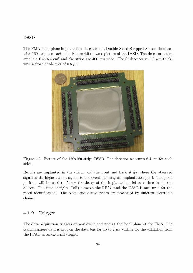
DSSD

The FMA focal plane implantation detector is a Double Sided Stripped Silicon detector,with 160 strips on each side. Figure 4.9 shows a picture of the DSSD. The detector activearea is a 6.4×6.4 cm2 and the strips are 400 µm wide. The Si detector is 100 µm thick,with a front dead-layer of 0.8 µm.

Figure 4.9: Picture of the 160x160 strips DSSD. The detector measures 6.4 cm for eachsides.

Recoils are implanted in the silicon and the front and back strips where the observedsignal is the highest are assigned to the event, defining an implantation pixel. The pixelposition will be used to follow the decay of the implanted nuclei over time inside theSilicon. The time of flight (ToF) between the PPAC and the DSSD is measured for therecoil identification. The recoil and decay events are processed by different electronicchains.

4.1.9 Trigger

The data acquisition triggers on any event detected at the focal plane of the FMA. TheGammasphere data is kept on the data bus for up to 2 µs waiting for the validation fromthe PPAC as an external trigger.

84

Thee are two types of event:

Decay event: A decay event is triggered by the overlap of a front and back signal in theDSSD decay channel. The event is built from the DSSD decay signals and comprisesthe pixel ID, the timestamp of the event and the energy in the DSSD. The Gamma-sphere signals have no trigger conditions (whether in time, energy of multiplicity),moreover, because of the calorimetric mode, there is no Compton suppression (butthe modules can be tagged as dirty offline).

Recoil Event A recoil event is triggered by a signal in the PPAC; it vetoes the trigger ofa decay event. Recoil events contains the PPAC information (X,Y, ∆E), the DSSDinformation (pixel coordinates, energy), the time of flight and the Gammasphereinformation, if any.

Figure 4.10 describes the trigger logic. During the experiment, the average global triggerrate was 170 to 180 Hz, with a DSSD event rate around 1 – 2 Hz.

85

Figure 4.10: Trigger logic schematic representation. The green lines represent the signalsread by the acquisition, the orange lines are the logical trigger signals. The two types ofevent are associated with different trigger signals. The PPAC signal triggers the readingof the Gammasphere information and the PPAC and DSSD recoil signals, while vetoingthe decay overlap trigger. The decay trigger initiates readout of the DSSD decay signals.

86

4.2 Recoil and recoil decay tagging

The very small cross section of the reaction makes it hard to observe 254No γ-rays at thetarget position, which we need for the calorimetric measurement. The information fromthe PPAC is not quite enough to unambiguously identify the nuclei of interest and to selectthe corresponding target-position events. The best signature of 254No is the α decay energyand half life. The correlation between recoils and subsequent decays over time allows theunambiguous identification of nuclei.

Target-position – focal plane correlation: Every implant event is associated withthe target-position events: γ energies detected by the Ge or BGO and time between thedetection in Gammasphere and the event trigger (PPAC signal). Implant events containthe relevant prompt Gammasphere data. The only additional selection needed is the timebetween the detection of the recoil at the focal plane and the detection of the γ-ray whichhas to be the time of flight of the recoil.

Pixel correlation in the DSSD: The high pixelization of the silicon detector leadsto a low rate of implant and decay in each pixel. With an average 200 Hz experimentalrate of DSSD implant, there was a rate of the order of 8 mHz implants per DSSD pixel;with an average decay rate around 2 Hz the average decay rate in a pixel is 80 µHz. Withan average 2.5 minutes between two pixel events and about 200 minutes between decays,there is enough time to observe two subsequent decays of 254No or its daughter nuclei(respectively 51 and 1800 seconds half lives).

The decays in the DSSD are correlated to a previous implant in the same pixel using thepixel coordinates. A time condition is put on ∆T1st decay = Tdecay − Timplant restricting theimplant-to-decay correlation time to a few half lives of 254No (T1/2(

254No) = 51 s) to avoidcorrelating with random events. One limit of the method is that the detection efficiencyof the α is about 55 % because the emitted α might escape from the silicon and leave onlya tiny fraction of its energy.

87

4.3 Calorimetric measurement

4.3.1 Principle of measurement

The calorimetric measurement with Gammasphere is done by using the BGO shields aspart of the detection system. We measure the total energy detected at the target positionand the number of Gammasphere modules that fired – the fold. We will need to calibratethe BGO energy reading precisely to find the original total energy and the number of γ-rays emitted by the nucleus. The calibration has been performed sector by sector with88Y, 203Hg, 207Bi and 137Cs sources, with energies at 898, 1836, 279, 569, 1063, 1770 and662 keV. See later section 5.1.1 for calibration.

Gammasphere module: hit

For calorimetric measurements, the number of hits is either one or zero for one module. Weconsider that a module has a hit if any of its BGO sectors or its Ge triggers are within theappropriate time gate. Two γ-rays interacting in the same module will therefore registeras one hit only. For the energy deposited in the module, the Ge and BGO energies areread and multiple gamma hits will naturally lead to the measure of the sum energy. Forthe purpose of calorimetric measurement, it has been shown it is not useful to separate Gecrystal, BGO shield and BGO sectors to increase the number of modules [85].

Selection of hits in time and energy

The γ-rays hits, whether in the Ge detectors or in the BGO, are selected according to thetime of the event, relative to the implantation of the recoil, in order to select precisely theγ rays associated with a recoil and not any γ from background or another reaction (seepreviously, section 4.2). It is also important to take the time walk of the time, coming fromthe charge collection dynamics or the leading-edge discriminator, into account. Figure 4.11shows the selection of events. The γ time peak is larger than for a source measurementbecause of the energy dispersion in the target, implying a dispersion in ToF.

Building the k and H quantities

The number of hits detected – the fold, noted k – and the detected energy – noted H – arebuilt off-line from the events selected as previously described. In one individual module i,

88

Figure 4.11: Selection of Ge (Top) and BGO (bottom) hits for the (k,H) distribution: thered lines are the banana gates. The low energy events are shifted to later times (smallerdifferences between global trigger and module trigger) due to the charge collection dynamicsor the leading-edge discriminator of the detector. The comparison with source data in figure4.12 shows that the gates are wide enough to account for the time walk.

89

Figure 4.12: Selection of Ge (Top) and BGO (bottom) on a 203Hg source: the red linesare the banana gates. The source emits a 279 keV γ ray that is perfect to check the timewalk. The red lines are the graphic selections applied to the experimental data, shifted tothe centre of the time peak. 90

the individual fold and energy, ki and H i, are built following three possible scenarios :

• Ge time in Cut AND BGO time in Cut: H i = EiGe + Ei

BGO, ki = 1.

• Ge time in Cut AND BGO time not in Cut: H i = EiGe, ki = 1.

• Ge time not in Cut AND BGO time in Cut: H i = EiBGO, ki = 1.

Afterwards, the global fold and sum energy are simply k =

i ki and H =

i Hi.

4.3.2 Partial loss of BGO and Ge signals

Electronic bus

The electronics has to hold the signal information (amplitude, time, ...) long enough towait for the delayed trigger signal coming from the PPAC at the FMA focal plane. TheFMA is 8.2 meters long, the recoil mass around 254 u and the average kinetic energy ofthe recoils is approximately 38 MeV; therefore it takes about 1.54 µs for recoils to fly fromout of the target chamber to the PPAC. The electronics bus is designed to keep the BGOsignal for 2 µs – but in reality, it is observed that some channels have a bus width as shortas 1 µs. For Ge & BGO modules with an early bus end (tend), signals coming after tend

are lost. For those modules, both the Ge and BGO information are lost, except in a fewcases where the Ge signal is still present. The loss of those information is linked to shortcables between the Gammasphere modules and the acquisition, leading to an early arrivalof the module signal and a bus signal not long enough to hold the electronics informationuntil the arrival of the focal plane trigger signal.

The spectra on figure 4.13 explains the issue: some modules are completely missing therecoil gated time peak. One can compute the fraction of the recoil time peak being lostby a module. Let Precoil be a normalised Gaussian distribution reproducing the recoil peak(see figure 4.14), the fraction of events seen by the BGO i is therefore fi =

tiend

0P (t)dt

(where tiend is the bus end time for modules i) – this way, we compare the data loss with areference time distribution for 254No recoils tagged γ-rays.

One can calculate that 80 % of the modules keep more than 90 % of the signal, and theglobal fraction of events kept ( 1

Nmodules

Nmodules

i=1 fi) is 80.5 %. This fraction of data lostis in agreement with the observed calorimetric efficiency of 63 %, compared to 78 % forsimilar measurement without the problem of module loss [89].

91

Figure 4.13: Visualisation of the early end of BGO bus. The blue spectrum of time eventshows a normal bus with time signal being detected up to more than 1800 ns. The redspectrum shows a bus with an early end with a significant loss of data after 1580 ns. Thegray area is the time peak of recoil gated events, corresponding to the gamma in the 254Noreaction

92

Figure 4.14: BGO (Top) and Ge (bottom) time spectra gated by recoils. One can seethe recoil peak around 1.54 µs at the end. The red line is a fit of the distribution witha Gaussian and a linear background. The Gaussian parameters are used to calculate thefraction lost for modules with a short bus signal.

93

Problem for response calibration

The information loss in the modules implies that part of the experimental data for k andH will be lost, while they will be present in the calibration data since these data aretaken from a source and without the issue of waiting 1.54 µs before a trigger. Indeed, thecalibration data has a peak centred of t = 0 ns. We devised two ways to take into accountthis problem.

Use of self-triggering Gammasphere To reproduce the condition of the experiment asclosely as possible in the response calibration, we took the source data with Gammaspheretriggering on an external signal, this signal was a delay of the OR of the modules. Withthat, we could set the delay up to 1.54 µs like it is in the experimental data and observedthe same loss of data in module buses. However, this method could not be used entirelydue to the poor statistics of the source data taken with a delay self-trigger, as we were notaware of the magnitude of the problem at the time.

Correction of source data To account for the partial loss of experimental data, wehave to remove the equivalent amount of data from the calibration data used to build theGammasphere response. As each detector sees a fraction of the signals in the experiment,we have to remove the appropriate quantity of data from the source.In the collection of fold and energy data from the source, we will randomly suppress eachdetector according to the fraction fi defined earlier: a signal in the module i will be masked(i.e. not read) with a probability 1 − fi. This decision is taken using a random numbergenerator, which provide a random float r between 0 and 1. If r ≤ fi the event is kept, ifr > fi the event is suppressed.

94

Chapter 5

Data analysis

5.1 Calibration of detectors

5.1.1 Gammasphere

Calibration of Ge detectors

Energy The energy reading from the Ge detectors of Gammasphere is processed byADCs and calibrated using 88Y, 207Bi, 60Co, 152Eu, 137Cs, 203Hg and 56Co source; exampleof background subtracted spectra are shown on figure 5.1. Each Ge crystal is calibratedby a linear function. This leads to a 2.6 keV resolution at 1.3 MeV. The average thresholdin the Ge detector is 40 ± 10 keV.

The background spectra are collected in between source runs. The background lines comefrom activation of the chamber and beam line during irradiation and also fission-productactivities. Some of the activities have quite short lifetimes and the corresponding back-ground lines are not properly subtracted out. However, this will have little effect on ourconstruction of the calorimetric response (see section 5.8) as coincidences between γ raysare used.

Efficiency The detection efficiency of the Germaniums is measured with 152Eu, 60Co,207Bi and 88Y sources.

95

Figure 5.1: Background subtracted spectra of the sources used for energy calibration ofGammasphere. 88Y (top), 207Bi (middle) and 60Co (bottom). The energy of the mainpeaks are noted in red.

96

Relative efficiency The relative efficiency profile is obtained by combining the γ

peaks areas information from sources, using the RADWARE gf3 and effit utilities [90].The profile shows a maximum efficiency around 270 keV and falling to half its maximumabove 1 MeV.

Absolute efficiency The absolute detection efficiency has been obtained at differentenergies using sources with coincident γ-rays, like for the Gammasphere response calibra-tion. In a source where two γ-rays γ1 and γ2 are emitted in coincidence, the number ofcoincidence detected is given by Nγ1&γ2

= Aλ(θ)ε1ε2 with A the source activity, λ(θ) theangular correlation function characterising the geometry of the γ emission. λ(θ) dependson the angle between the two γ-rays (averaging to 1 over all the Gammasphere detectorscombinations). εi, the detection efficiency at the energy Eγi

, verifies Nγi= Aεi, with

Nγithe number of full-energy Eγi

detected. Therefore, the ratio Nγ1&γ2/Nγ1

= ε2 – aftercorrection for angular correlation and possible non-100% correlation between gamma-rays(for example, converted transition in the 207Bi). Table 5.1 give the values obtained withthis method. This method works best for two γ-rays of close energies.

Source Energy E2 (keV) Coincidence Nγ1&γ2Number γ1 Nγ1

Efficiency ε2 (%)152Eu 121 3256 ± 57 19151 ± 44 17.0 ± 0.3152Eu 344.8 27800 ± 260 142050 ± 380 19.7 ± 0.2207Bi 570.1 142050 ± 1625 918800 ± 960 15.4 ± 0.288Y 898.4 101940 ± 1190 903710 ± 950 11.3 ± 0.1560Co 1332.8 57415 ± 1085 602555 ± 365 9.5 ± 0.288Y 1836.4 122280 ± 1155 1436900 ± 1200 8.5 ± 0.1

Table 5.1: Absolute efficiency extracted from coincident γs data.

One can also get an absolute efficiency values by examining the sum peak for sourcesemitting 2 coincident γ-rays, when they are detected in the same detector. The probabilityof detecting both γ1 and γ2 in the same detector is given by λ0ε1ε2 where λ0 = λ(θ = 0).The ratio of sum peak intensity and single γ intensity, corrected for λ0 is therefore a simpleway to measure the efficiency [91]. In 60Co, the λ0 coefficient is 1.074 [92].

Figure 5.2 shows the absolute efficiency profile with the experimental data points.

Energy in the BGOs

For our calorimetric measurement, we need to get the BGO sectors calibrated in energy.

97

Figure 5.2: Absolute efficiency profile for Gammasphere. The black points are the absoluteefficiency measurement from correlated γ rays. The red points are the points used forrelative efficiency calibration, scaled down to match the absolute efficiency measurement.The blue line is the relative efficiency profile scaled down to the absolute values.

98

The energy read in each sector is not directly available from Gammasphere. Only the sumof all sectors is given, and the hit pattern indicates which sectors fired. By selecting specifichit patterns, sectors were calibrated one by one with the same sources as Ge crystals, seefigure 5.3 and 5.4.

Figure 5.3: Fit of the BGO energy, on a 88Y source. The seven sectors spectra are alignedand overlaid at the bottom. The module energy is fitted.

In cases where more than one BGO sector fires, we divide the sum signal equally betweeneach sector and used the calibration on each sector. The final energy resolution of theBGO is around 120 keV at 570 keV and 200 keV at 1.3 MeV. The relative resolution isabout 20 % FWHM. The average threshold in the BGOs is 120 ± 30 keV.

Time

To analyse the γ-rays, one has to select the hits corresponding to a specific beam burst.Each Ge and BGO channel has its own TAC that gives tGe and tBGO – see section 4.1.6for description. The TAC channels have to be aligned and calibrated. The time alignmentis performed using Gammasphere self-triggering on the delayed OR of all modules. Withthat, it is easy to get a set of values of times between γ detection and trigger. Using

99

Figure 5.4: From top to bottom: 88Y, 60Co and 207Bi sources. Overlay of calibrated BGO(orange line) and Germanium (blue line) energy spectra.

100

different values of delay, the linearity of the time signal in the modules is calibrated. Toaccount for the width of the peak, we choose to offset the time t = 0 by 1000 ns. Figure 5.5shows the alignment of Ge time signals. The similar process has been made for BGOs.

Figure 5.5: Time distribution of events for a 88Y source. The uncalibrated time is onthe left, the aligned time on the right. (Top) distribution of events for each Ge detector.(Bottom) projection of the total time distribution. The data compression (bin width)differs between calibrated an uncalibrated spectrum.

101

5.1.2 DSSD calibration

Decay channels

The DSSD decay channels have been calibrated using an external α-source and the α-decays of reaction products implanted in the silicon during the experiment – in particularduring the test reaction, see section 5.3.

The channel alignment is done with a classical 3-α source, whose energies are well tabulated– see table 5.2. Because the α from the source have to go through the detector dead-layer,the energy loss in it is taken into account. The source is located about 20 cm in front of theDSSD, therefore the effective dead-layer is at most 2 % thicker for the pixels on the edgeof the silicon; no correction for the pixel location is made since the difference in energy issignificantly smaller than the resolution.

Radio nuclide α Energy (MeV) α energy after the DSSD dead-layer

240Pu5.105 5.005.156 5.05

241Am 5.485 5.39

244Cm5.763 5.665.805 5.70

Table 5.2: α energies in the PuAmCm 3-α source. We give the energies of the α and theenergy deposited in the active volume of the DSSD after an energy loss in the dead-layer.

After aligning the channels, the experimental decay of implanted nuclei is used to set theenergy scale. The final energy resolution is about 35 keV FWHM. Figure 5.6 shows thecalibration of the front and back side of the DSSD with the α source.

The DSSD events are triggered by an overlap between the front and back strip withina 250 ns time window. Even if the two sides of the DSSD are calibrated, we will usethe measurement from the front side which is more precise because the recoil nuclei areimplanted in the front side (The average implantation depth is below 5 µm). Hence, thedecays happen mainly close to the front strip and the charge carriers have to drift to theback side through a larger thickness of matter and are spread between strips at the back.Figure 5.7 shows the calibrated front and back energy for the experimental decay of 254No.The better charge collection on the front side is clearly illustrated by the tails on the leftside of the diagonal.

102

Figure 5.6: DSSD channels front (right) and back (left), before (top) and after (bottom)channel alignment with 3-α source. The uncalibrated spectra show important numberof counts at low energy, implying the need of significant thresholds: the average energythreshold is 160 ± 15 keV.

103

Recoil channels

As for the decay, the recoil energies have been calibrated too. The implantation energy inthe DSSD is around 30 MeV, but the dynamic of charge creation in the silicon reduces themeasured energy: around the implanting ion, a plasma is created and the holes-electronpairs recombine before being collected. This effect called Pulse Height Deficit reduced themeasured energy by about 50 % [93].

For the recoil calibration, the gains has been aligned with a pulser and the 3-α source hasbeen used to set roughly the energy scale.

104

Figure 5.7: Plot of the front vs. back energy in the DSSD for experimental 254No α decayswith no conditions on the signals. The front side sees more energy than the back side.

105

5.2 Recoil selection at the focal plane

The FMA transports to the focal plane all recoils of a given m/Q. The recoil velocitycan also be used for extra selection via the time of flight. At the target position, 254No isproduced and enters the FMA. We set up the FMA to transmit the charge state 20.5+ atthe centre of the focal plane, charge states Q = 20+ and Q = 21+ will be collected. Alongwith 254No, all particle with m/Q around the set up value ( 254

20.5≈ 12.4) will be transmitted,

although with a different mass, kinetic energy, time of flight, ... Therefore, separation ispossible using the following measurements :

• X dispersion in the horizontal direction at the focal plane, corresponding to the m/Q

ratio, measured by the PPAC.

• Time of Flight (ToF), between the PPAC and the focal plane DSSD.

• Energy Loss in the PPAC (∆EPPAC).

• Implantation Energy in the DSSD (Eimplant).

5.2.1 Contaminants

Given the low production cross section of 254No, the nucleus of interest is a small fractionof all the recoils getting to the focal plane. It is therefore very important to sort throughall the events at the focal plane. Three types of elements gets to the focal plane:

• The nuclei of interest: 254No.

• Target like products: scattered target and transfer products (Pb, Po, Bi, ...).

• Scattered beam and beam like products from transfer reactions.

Beam like products

The scattered beam and beam like products undergo multiple scattering in the target andon the walls of the FMA. Therefore their charge state and energy are not well defined.However, we know they are light (A around 48) and very energetic, therefore fast. Thescattered beam will be characterised by a high and broad recoil energy, a low ToF and alow energy loss in the PPAC (because of the Bethe-Bloch formula : ∆EPPAC ∝ AZ2

Eimplant).

106

Furthermore, the scattered beam will be the dominant contaminant, by many orders ofmagnitude.

Target like products

In the target, the 208Pb atoms may undergo elastic scattering giving them a kinetic energyof about 40 MeV. Also, inelastic reactions between the beam and target may lead to transferproducts with A ≈ 208 scattering to the focal plane. The heavy mass of the target elementwill lead to a ToF lower but of the same order of magnitude than the ToF of the recoils ofinterest; the energy loss in the PPAC will be less than for 254No.

5.2.2 254No recoils

The kinetic energy of the 254No recoils is around 38.7 MeV for Ebeam = 223 MeV (38 forEbeam = 219 MeV). The recoils are heavy (the heaviest of everything that gets to the endof the FMA) and with a large Z (102, charge state around 20+). The time of flight of 254No

recoils will be about the same as forward scattered target atoms (since v =

2·KM

– withK the kinematic energy of the recoil and M its mass, the ratio of scattered target speedover recoil speed is ≈

KPb

208254KNo

≈ 1.13). However, the energy loss in the PPAC will belarger for the Nobelium recoils due to the higher Z.

5.2.3 Cuts and Selections

The selection is made by combining several cuts on the quantities. To be more selectivewithout cutting the events of interest, the 2D plots and banana gates are preferred. Tovisualise where to put the gates, it is helpful to plot decay tagged events (see section 4.2).

Primary selection: data completion

The first selection on all the events is to make sure all the needed quantities are available.Due to thresholds in the detectors and electronics, some events are incomplete: quantitiessuch as X or Eimplant are 0). A proper selection is impossible for these events. Table 5.3gives the selection budget with the count of valid events. A large fraction of events have∆EPPAC information missing, therefore, this quantity has been removed from the comple-tion selection, and these events were kept.

107

Condition Number of recoils %

No Selection 100116 100Invalid ToF 4482 4.5Invalid Implant Energy 2288 2.3Invalid X,Y 0 0Any Invalid parameter 30261 8.2

Valid Events 91106 91In Eimplant-ToF 3105 3.4In X-∆EPPAC 3644 4In Eimplant-ToF and X-∆EPPAC 915 0.91

Table 5.3: Selection budget for the data set at EBeam = 219 MeV. The number of event ofinterest is just a fraction of the total.

Time of flight and implant energy

The time of flight and energy of the implanting recoil are two very selective parameters,since they are tied in the kinematic relations by the mass of the recoil: ToF = L

m2Eimplant

,

with L the distance of flight.

Figure 5.8: Selection of recoils on the Energy, Time of Flight map. The black line is thegraphic cut applied to select recoils. The red points are the α-decay gated events.

108

The distribution of events on a (ToF, Eimplant) plot gives a large group of events witha broad recoil energy distribution and a long time of flight. We associate this with thescattered beam and light transfer products. Above the scattered beam, events with higherToF are associated with heavier recoils (longer flight for the same energy). Figure 5.8shows the selection of events on the Energy, Time of Flight map.

Energy loss in the PPAC and X position

The energy loss in the PPAC and the X position at the FMA focal plane provide additionalselectivity according to charge state and mass. The FMA is set on a precise value of m/Q.The distribution of (X, ∆EPPAC) shows the recoil of interest with peaks in the X directionand ∆EPPAC somewhat larger that the beam and target-like recoils. Combining the PPACenergy loss with the ToF measurement (which is also related to the recoil energy and mass)gives a way of identifying the recoils – figure 5.8. The 254No recoils are expected to havelarger ∆EPPAC than scattered beam and target. Figure 5.9 gives the selection of events onthe X, ∆EPPAC map and figure 5.10 gives the selection of events on the X, Time of Flightmap.

Figure 5.9: Selection of recoils on the X and Energy loss map. The black lines are thegraphic cuts applied to select recoils. The red points are the α-decay tagged events.

Figure 5.11 shows the final X distribution of the selected events. It shows the two chargestates peaks for Q = 20+ and 21+. The peak at higher X is smaller because of a poorer

109

transmission of those charge states in the FMA and smaller population of the Q = 21+

charge state.

110

Figure 5.10: Selection of recoils on the X and Time of Flight map. The red points are thedecay gated events. The black lines represent the selection.

Figure 5.11: Selection of recoils in X. The black histogram is the distribution of X for allthe PPAC events, normalised to 1. The red filled histogram is for decay tagged events, itis scaled up by a factor 10 (unscaled integral is 0.0097).

111

5.3 Test reaction: 176Y b

48Ca, 4 − 5n220,219

Th

We tested the setup using a reaction with a larger cross section. We chose to produce220Th because in addition to presents prompt γ-rays and α-decay its entry distribution hasbeen measured previously with the same setup and presents a good comparison point tovalidate the calorimetric measurement – see appendix C.

5.3.1 Reaction and production cross section

The 48Ca + 176Yb reaction is not the preferred way to produce 220Th but it has a largecross-section (compared with the production of 254No) and has the advantages of using thesame beam and same energy as for the 208Pb(48Ca, 2n) reaction. However, at this energy,both 220Th and 219Th are produced at the same time with cross sections of the order of 10to 100 µbarns.

During a little less than one day (≈ 17±2 hours) of test run with a beam intensity averaging30 pnA, we accumulated about 3950 219,220Th events, which, assuming a 7 % transmissionefficiency through the FMA gives 20 ± 10 µbarn in agreement with the production crosssection values.

5.3.2 γ and decay spectroscopy of 220Th

The two isotopes 220Th and 219Th can be separated on the X distribution (see figure 5.12)and we can check the γ spectra associated with each. In particular, the 220Th X-gatedspectrum is in agreement with references [94]. See figure 5.13 for the spectrum.

The Thorium isotopes produced are implanted in the DSSD at the FMA focal plane andundergo α decay inside the DSSD. One can follow the decay and identify the decayingnuclei by the combination of decay energy and half life – see section 4.2 and figure 5.14.However, the short lifetimes of the species (≈ 1 − 10 µsec) make it difficult to observeall the decays. It is possible to identify clearly the decays of 215Ra and 212Rn by their α

energies and half-lives, as shown on figure 5.15.

112

Figure 5.12: Distribution of X positions for 219,220Th recoils. The two isotopes can beseparated in mass, in particular at low Xs where there is more population. The line in blueshow the distribution for 219Th and the one in orange for 220Th.

Figure 5.13: Prompt γ rays spectrum for 220Th. The known transition energies are markedin red, following [94]. The corresponding level scheme is on the right. Two higher energylines come from 219Th, marked in blue.

113

Figure 5.14: Decay path of 220Th (orange) and 219Th (blue). The half-life of nuclei arewritten in the squares. The red arrows represent electron capture decay. The black arrowsstand for the α decay, with the tabulated α energy in MeV indicated over the arrow. For211Rn and 211At, the size of the arrow indicates the branching ratio between the two decaymodes.

114

Figure 5.15: Energy and time of the decay of 215Ra (top) and 212Rn (bottom) inside theDSSD. The selection on the two decays have been done by correlation time condition. Theα energy and lifetime correspond to the expected values of 8.7 MeV and 1.6 ms for 215Ra,and 6.2 MeV, 24 minutes for the Rn isotope.

115

5.4 Cross section

The first quantity we check in the data collected for 254No during the experiment is theproduction cross section at the two energies.

We collected respectively 915 ± 40 and 1475 ± 60 events for the experiment at 219 and223 MeV (uncertainty comes from the data selection); assuming a transmission cross sectionfrom the target position to the FMA focal plane of 7%, with a beam exposure of 43 hoursat EBeam = 219 MeV and 118 hours at EBeam = 223 MeV, with an average beam intensityof 10 pnA, and a duty cycle of 73% (due to the target wheel spokes), plus a 60 % efficiencyof recoil tagging at the focal plane – due to geometrical consideration, the focal planechamber being not setup in the most ideal configuration during the experiment – we canestimate the production cross section of 254No. Table 5.4 gives the results and comparethem to references. See also figure 5.16.

Beam Energy (MeV) Counts Observed σ (µbarn) Expected σ (µbarn)219 915 2.1 ± 0.6 1.85

223 1475 1.2 ± 0.4 1.15

Table 5.4: Summary of observed 254No production cross section compared to the references.Expected cross section are taken at the mid-target energy.

Figure 5.16: Plot of the 254No production cross section — red line is the reference calculatedby the NRV code [9]. Black points are our experimental value, with energy taken at mid-target.

116

5.5 Prompt γ spectroscopy

The prompt γ information collected during the experiment allows us to check the pro-duction of 254No and also to directly observe the spin population via the yrast decaysassociated with known angular momentum [25, 26, 95–97]. Figure 5.17 shows the recoil-gated γ spectrum for all data. Figure 5.18 shows the spectra at both beam energies.

Figure 5.17: Recoil-gated γ ray energy spectrum for all data (EBeam=219 MeV and EBeam =

223 MeV). The known yrast transitions γ energies are marked in red; 254No X-rays aremarked in blue. We observed the yrast transitions up to 14+. The ratio of 254No X-raysto the peak at 600 keV in the spectrum is 4.3± 1.2, consistent with the spectrum collectedduring the previous experiment where it was 5.3 ± 1 [98].

Decay-gated spectra In order to remove background and close in on the 254No data, wecan use additional conditions in the γ ray spectrum. In particular, recoil-α and recoil-α-αcorrelation. The additional condition removes background, but it also reduces the statisticby the efficiency of α or α− α detection, for example. Figure 5.19 shows the γ spectra forrecoil-gated, recoil-α gated and recoil-α-α gated events.

Spin population

Since we are interested in the spin distribution of formed 254No, we can get a first estimateof the profile by looking at the yrast transitions and their intensities. Once corrected forefficiency and electron conversion, it is a good measure of how much of the nuclei were

117

Figure 5.18: γ energy spectra for the two beam energies: EBeam = 219 MeV (top) and223 MeV (bottom).

118

Figure 5.19: γ energy spectra for different conditions. From top to bottom: Recoil-gated,Recoil-α gated, Recoil-α-α gated.

119

formed at a given spin. Figure 5.20 gives the intensity profile for the two beam energies ofthe experiment; it shows the population stays above 20 % up to spin ≈ 18 . No sizeableincrease at high spin is seen between the two beam energies.

Figure 5.20: Intensity in each yrast transition, corrected for detection efficiency and conver-sion. The black points correspond to data taken from a high-statistics spectrum measuredwith Jurogam [31]; red for the data set at EBeam = 219 MeV and blue for EBeam = 223 MeV.The values are normalised to the 8+ → 6+ transition (Eγ = 214 keV). The data combineour experiment and a previous measurement at the same energy.

5.6 Alpha spectroscopy

5.6.1 Decay chain

The implantation of 254No recoils in the DSSD pixels allows to follow the decay path overtime. Figure 5.21 shows the decay path of 254No; due to the low statistic of the events,only the α branch is visible, the small electron capture branch is too weak.

Contaminants from test-reaction: Decay products from the test reaction (219,220Th)have a long combined half life (several hours and more). Their decays are visible in thealpha spectrum. When looking at the spectrum run-by-run, one see that the intensity ofthese contaminant-peaks decreases.

120

Figure 5.21: Decay path of 254No, with the α energies and nuclei half-lives marked. 254Nopresents a small branch (≈ 10%) of electron capture leading to the α decay of 254Fm,however, the small probability should not lead to any significant peak. The decay chain isstopped by nuclei of very long half lives.

121

End of the decay chain: 246Cf decays with a half-life of about 1.49 days into 242Cm –that explains the lower population of the peaks – and 242Cm with a half-life of 162 days,hence, the Cm decay at Eα = 6.1 MeV is not visible. That reduces the observation of suchdecays and the ability to correlate them over time. Over an 8 hours window (the averagelength of an acquisition run), only about 14% of 246Cf events can be correlated. However,on a course of 7 days (total duration of the experiment) we will see about 90% of the 246Cfdecays, therefore, the uncorrelated decay spectrum should show the corresponding events.

Figure 5.22 shows the energy spectrum in the DSSD.

Figure 5.22: α energy spectrum for all decays in the DSSD, with no conditions. The threedecays associated with 254No are visible, in addition to long lived products of the testreaction.

5.6.2 Decay energy and time

The α-decay is characterised by an energy and a half-life, both being tied together (seesection 1.2.3). One can plot the map of decay energy and Log(∆T ) which is a very nice wayto identify the groups of specific decays. The maximum of the events Log(∆T ) distributionrelates to the half-life of the decay as described in [99,100].Figure 5.23 shows such map for the alpha decays for 254No, and figure 5.24 shows the samefor the decay of 250Fm.

The half-life of each nucleus can be measured from the implant-decay and decay-decaycorrelations. Table 5.5 gives the measured half lives compared to the references.

122

Figure 5.23: α energy and log of the time difference between recoil implantation and thefirst decay in the DSSD. 254No is clearly identified, as are the isomer events. At lowerenergy than the 254No αs, events with life-time in agreement with 250Fm are seen: theycorrespond to correlation for which the decay of 254No was missed.

Nucleus Measured Half-life Reference254No 52 ± 3 s 51 s250Fm 29 ± 7 min 30 min246Cf 35.7 h

Table 5.5: Summary of the measured half-lives for the 254No α, and the decay of daughternuclei. Uncertainty on 250Fm come from 211Po contamination.

123

Figure 5.24: α energy and log of the time difference between first decay and second decayin the DSSD. 250Fm is clearly identified.

124

Correlation deficit from implant to decay In the DSSD events, we observe that only40 % of the 254No decays – identified by the full α energy (8.1 MeV) – are correlated toan implant event. In the same way, 26 % of the 254No decays are correlated to a 250Fm(full energy), while 55 % are expected. There is a ≈ 50 % correlation deficit betweenrecoil-decay and decay-decay events.We tried to understand the origin of the issue, in particular, we investigated the possibilityof a recoil-decay electronic mapping mismatch (since recoils and decays have differentelectronics); but nothing supports this hypothesis. It is not a threshold effect since thedeficit is seen at high energy. We also tried to locate subsequent decays in neighbouringpixels, but this did not solve the problem.It is possible that a bad front-back signal overlap, required for decay and recoil events inorder to locate the pixel, is at the origin of the problem.

5.7 Isomer decays

There are two known isomeric states in 254No:

• One 2 quasi-particle K=8 long lived isomer identified at Argonne and Jyväskylä[40, 101] and confirmed by Berkeley and GSI [95, 97]. This isomeric state is highlypopulated (about 30 %).

• A short lived isomer at higher energy, less populated. It is likely a 4 quasi-particleexcitation with K > 14.

It is also possible to observe isomer decays in the DSSD. If 254No is implanted in theDSSD in an isomeric excited states, the subsequent decay to the ground state will produceconversion electrons, Auger electrons and X-rays. Those will contribute to a low energysum signal (a few hundred keV) [102] that can be detected in the DSSD. Unfortunately,our high thresholds made the detection of isomer decay events difficult and only a few ofthose events were seen.

In figure 5.23, we see the two event groups corresponding to isomer decay; it will bepossible to select specifically isomeric events by putting a gate around these points on theplot. Table 5.6 gives the half-lives found for the isomer.

125

Isomer Measured Half-life ReferenceLong lived isomer 298 ± 75 ms 266 ± 10 msShort lived isomer 113 ± 63 µs 171 ± 9 µs

Table 5.6: Summary of the measured half lives for the 254No isomer decays (referencefrom [40,95,97,101]).

126

5.8 Principle of calorimetric measurement and calibra-

tion

The calorimetric measurement gives the number of emitted γ transitions in the nucleus(multiplicity) and the associated total energy: m and Etotal

γ . Although Gammasphereis a great detector is not perfect and the measured quantities: k (the fold) and H (themeasured energy) are correlated to m and Etotal

γ but not in a simple way. In fact, therelation is neither direct nor reciprocal: to a given m correspond several k and a given k

can be detected associated with different values of m – same for the energy. Therefore, itis impossible to simply associate each 254No event to a

m, Etotalγ

. We have to work witha global distribution and averages. We will use a statistical method that will reconstructthe most likely

m, Etotalγ

distribution that leads to a given (k, H) distribution.

5.8.1 Measured quantities

Energy

The quantity H is the total energy measured by Gammasphere for a 254No event. Due tothe limited detection efficiency of the HPGe crystal (maximum ≈ 22% at 300 keV and 10% at 1.3 MeV), we rely also on the BGOs to measure this energy. In our experiment, thetotal detection efficiency was 63%.

Fold

k is the number of measured hits in Gammasphere, defined as one module firing within agiven time window and with an energy over the thresholds (see section 4.1.6). One notesthat a hit will correspond to a wide range of BGO sector and Ge firing combinations. Itis important that the time window and hit definition stays the same for calibration andmeasurement.

5.8.2 Fold and Energy calibration

The fold and energy response of Gammasphere to events of given multiplicity and energy(m, E) is calibrated using sources with coincident γ-decays. In practices, one uses a sourceemitting two γ-rays γ1 (E1) and γ2 (E2) with an (ideally) 100% correlation and gates on

127

the full energy detection of γ1 in any one Ge detector. Whatever is detected in GS incoincidence is the response of Gammasphere to one γ-ray of energy E2. The coincidencerequirement removes practically all the background from the relevant source spectra.

Figure 5.25: (Left) Coincident γ decays, schematic level and decay scheme showing theideal case of fully correlated decays. We use sources with decay pattern close to this tocalibrate the fold and energy response of Gammasphere. (Right) Response calibration inGammasphere: γ1 is gated on with Ge detector (in blue) and γ2 is detected (or not) bythe rest of Gammasphere (the separation of BGO and Ge is not represented).

We calibrated the response in fold and energy, with 88Y, 60Co, 207Bi and 152Eu. Table 5.7gives the sources used for calibration and the energies of the γ-rays involved in the cali-bration and figure 5.26 shows the decay pattern of the sources.

One has to correct the number of γ-rays observed for the branching of decay to the levelsinvolved in the cascade used for the response calibration and also for possible electronconversion of the transition. Table 5.7 shows the correlation and conversion factor for theused sources. The correction factor (= Nγ2

/Nγ1) accounts for the difference between the

number of gated γ1 and the expected number of emitted γ2. Those have to be taken intoaccount in building the response.

An additional correction has to be applied for the fact that one module is blind because itis gating on the γ1 transition (a clean Ge is required, i.e. no hit in the surrounding BGO).Therefore, the probability of missing one γ is increased by a factor 1/Ndetectors.

128

Figure 5.26: Level and decay scheme of the sources used for response calibration. Onlythe levels and γ-rays of interest for the response calibration are shown. The γ transitionmarked in red are the ones on which we gate to build the response.

129

Source E1 (keV) E2 (keV)Correlationfactor (%)

γ2

Conversioncoefficient

Global correctionfactor (%)

88Y 1836 898 94 < 0.0005 9460Co 1173 1332 100 < 0.0005 100207Bi 1063 569 100 0.0217 97.9152Eu 778 344 100 0.0398 96.2

Table 5.7: Correlation and conversion coefficients for the source used for response cali-bration. The global correction factor Nγ2

/Nγ1gives the ratio of expected calibration γ2 in

respect to the number of gated γ1.

Event Mixing method

To build the response matrices to multiplicities higher than 1 and energies larger than Eγ2,

an event mixing technique is used. With this method a pseudo event of multiplicity Mis built by grouping M one-γ events into a one M-γs event. In other words, for an eventof multiplicity M and energy M · Eγ2

, we consider a set of M events of multiplicity and

energy (1, Eγ2) and sum the measured energy : H(M,M ·Eγ2

) =M

1

H(1,Eγ2). For the fold of

the (M, M · Eγ2) event, the k of the pseudo-event is not the sum of individual ks but it is

built from the list of IDs of the modules contributing to the fold to account for the factthat k = 0 or 1. In this method, the correction coefficient from table 5.7 and the correctionfor the blind module are a scaling of the axes, done after the response building.

Random Generation

One can reduce the dependence on a limited number of events and implement the correla-tion and conversion corrections in a different manner by reproducing the characteristics ofindividual events from the one-γ fold and energy spectra. In practice, the individual fold(k) and energy (H) of a pseudo event is not read from the data but randomly selected fromthe distributions of those quantities. In this method, the correction of the spectrum for themissing γ-rays from non-100% correlation and conversion electron is done by down-scalingthe counts in the k = 0 and H = 0 bins of the spectra. This method offers an unlimitednumber of events by sampling the distributions. The IDs of the module triggering are alsosimulated using such statistical method, in order to correctly reproduce the experimentand account for the blind module.

130

Comparison of the two methods

Figure 5.27 shows the responses from the two methods. Although they are very similarthe randomly generated response is slightly under the event-mixing one.

Figure 5.27: Comparison of the responses – energy (top) and fold (bottom) – built by eventmixing (blue) and random generation (red). The responses are very similar, however, smalldifferences are visible : the randomly generated response is slightly below the event mixingone, it is particularly visible at high energy and multiplicity.

The single γ events used to make the response, are the same, except for corrections for thebackground and correlation correction. For the event mixing, correlation corrections arean axis scaling while the statistical method allows a better correction by applying themfrom the source. Furthermore, the background, particularly visible at high energy, can beremoved in the statistical method, which cannot be done in event mixing – see figure 5.28

131

Figure 5.28: Distribution of fold (top) and energy (bottom) of one γ events used to build theresponse by event mixing (blue) and random generation (red). The background subtractionat high energy and fold is clearly visible. One should note the high number of counts at 0in the H spectrum.

132

Random γ contribution We want to determine the importance of the contribution of γ-rays from background radiation, multiple reactions in the same beam burst (the probabilityof a fission reactions at the same time as the formation of a 254No is about 2 %), ... to the(k,H) distribution.The average rate of γ events in the Ge detectors of Gammasphere being RγGe ≈ 12 kHz,accounting for the average multiplicity of events (M = 6), the module detection efficiencyεmod ≈ 80 % and a 140 ns time window, we expect an average RγGe × M × εmod

εGe≈

0.07 random γ/recoil. This number is consistent with what is seen in the data. In plotslike in figure 4.14, we extract from the background at low times a rate of randoms of ≈0.5 10−3 /ns, or ≈ 0.04 random γ/recoil. The contribution of randoms to the measurementis weak, of the order of a few per cent, but can not be neglected. Moreover, the energycontribution of random γ-rays is unknown and hard to quantify.

Mathematical parametrization

The shape of the responses is rather simple and can be parametrized assuming a Gaussiandistribution with the centroid and width functions of the energy or multiplicity :

(H, σH) =

H0 + b · E,

σ20 + (σ1 · E1/3)2

(5.1)

(k, σk) =

N

1 −

1 − ε

N

M

,

σ20 + (σ1 · M1/3)2

(5.2)

In equation 5.1 the average energy H is a proportional to the total energy emitted E. Inequation 5.2 the average fold is determined by the number of modules N , the multiplicityof events M and the multiplicity efficiency ε and can be seen as a probability of not missingk out of M events in N detectors. The width parametrization is arbitrary. The modellingis a simplification and can not be used as a proper method to build a response. However,the mathematical formulae, in particular for efficiency, is a good way to characterised aresponse.

5.8.3 Response characteristics

For different energy

The simplest way to characterise the response is to look at snapshot quantities, for givenvalues of the multiplicity and energy, the distribution of relative fold (k) and observed

133

energy (H) is a good value to look at. These quantities follow the same pattern: the relativefold (k/M) and energy (H/E) increases from low values (≈ 35 %) for low γ energies, peaksat ≈ 60 − 75 % around 800-1000 keV and decrease for higher energies. Figures 5.29 showthis evolution. The rise of efficiency with energy at low energies is due to the detectionthresholds and the low probability of scattering. We see that the fold response saturates athigh energy while the energy does not. The decrease in energy efficiency is possibly linkedto the missing modules since γ-ray scattering becomes more important at higher energy.

Figure 5.29: Relative fold (k/M) [Top] and energy (H/E) [Bottom] for different sourcesused for the response, at multiplicities 5 (blue), 10 (red) and 15 (green), plotted as afunction of the energy of the γ-ray detected in the one-γ events (the points are slightlyshifted proportionally to the corresponding multiplicity to distinguish them).

There is small dependence of the relative fold and energy measurements with increasingmultiplicity (see figure 5.29). This evolution is much less significant than the energy depen-dence, and the decrease in detection efficiency with increasing multiplicity can be explainedby the fragmenting of the total energy into several γ-rays. This shows that there is a cleardependence of the response on the energy of the γ-rays, while the multiplicity does not

134

change the response in any significant extent. This is expected since detector thresholdsand scattering depend very much on the energy of the γ-rays.

Decoupling of fold and energy response

As we saw previously, the energy of the γ ray used for the response calibration changesthe response in multiplicity and energy. So far, however, we have considered these twoquantities to be independent. This goes against the natural idea that the response to oneγ-ray of very high energy will differ from the one for many γ-rays of small energies.

In a very complex γ environment, with a broad distribution of multiplicities and γ energies,it becomes virtually impossible to calibrate the response to match perfectly the experimen-tal conditions and we have to rely on our best estimate of the fold and γ energies to pick theadequate source to build the response – nothing is against using the multiplicity responseform one source and the energy response from another – to match as best as possible theexperimental conditions. We choose to use the response from 88Y because the averageγ energy detected in the Ge and BGO detectors is of the order of 900 keV. For this re-sponse, the energy efficiency is 63 % and the multiplicity efficiency,obtained from a fit ofthe average k as a function of M as in equation 5.2, is 71 %.

The best way would be to calibrate in a 4-dimensions space (E,M, H, k) and not two 2-dimensions spaces as we do (E,H), (M, k). But the unfolding in 4D would be very hardto perform since no source allow us to control independently E and M; moreover, theunfolding would become extremely long due to the bi-quadratic size of the space neededto solve the unfolding system.

5.9 The unfolding procedure

To go from the (k, H) distribution to (M, E), one has determine the original distributionwhich gave the measured (k,H). The relation k → m and H → E is not straightforward,therefore, a stochastic trial and error method is used. This method will allow the recon-struction of the most likely distribution of multiplicity and energy (M, E) that would leadto the observed (k,H) distribution.

135

5.9.1 Principle of the unfolding

The response matrices only allow the transformation from multiplicity to fold or energyto observed energy (H). The unfolding process will therefore rely only on the M → k andE → H direction. This method has been described in [103, 104]. The iterative processfinds the relevant (M,E) points that, once folded, give a (k,H) combination that is inthe measured distribution. Repeating the operation until all the (k,H) points have beenmatched by a (M,E) point, the whole distribution is unfolded. The final (M,E) distributioncontains the points that reproduce the measured (k,H) distribution.

5.9.2 Formal description of the unfolding

In mathematical terms, the unfolding involves the following quantities:

• Nfolded(k,H): the number of counts in the folded distribution at fold k and observedenergy H; this is the experimental measurement.

• PM(k) the probability distribution of k values associated with the multiplicity M .

• PE(H) the probability distribution of H values associated with the energy E.

• N (i)(M, E) the number of counts in the unfolded distribution at multiplicity M andenergy E for the unfolding iteration i.

The goal is to get the unfolded distribution Nunfolded(M, E) so that Nfolded(k,H) =

M,E

Nunfolded(M, E)

× PM(k) × PE(H). The unfolding iteration represented in figure 5.30, follows these steps:

• Starting from a test distribution N (i)(M, E), we prepare an empty next-iterationN (i+1)(M, E).

• As long as

M,E

N (i+1)(M, E) <

M,E

N (i)(M, E), the following loop is performed:

– Test multiplicity and energy Mtest and Etest are random obtained from the dis-tribution of N (i)(M, E) ((a) in figure 5.30).

– If N (i)(Mtest, Etest) > 0 :

∗ The associated ktest and Htest are randomly obtained from the distributionsPMtest

(k) and PEtest(H) (step (b) in figure 5.30).

136

∗ If Nfolded(ktest, Htest) > 0 :

· Counts of Nfolded(ktest, Htest) is decremented by one ((c) in figure 5.30).

· Counts of N (i+1)(Mtest, Etest) is incremented by one ((d) in figure 5.30).

Figure 5.30: Schematic view of one unfolding step: A test multiplicity Mtest is randomlyselected (a), and a test fold ktest is obtained from the response at Mtest (b). If The folded(experimental) distribution has a count at ktest, the experimental distribution is decre-mented at this fold (c) and the unfolded distribution is incremented at Mtest (d). Thelimits in the experimental distribution (kmin and kmax) determine the limits on multiplicityto consider Mmin and Mmax

The starting distribution N (0)(M, E) is arbitrarily set to a uniform distribution; it hasbeen observed that unfolding procedure converges after only a few iterations. A uniform

137

distribution is therefore good enough and has the merit of introducing no bias in theunfolding by letting all the (M, E) space open for the final distribution. The range of Mand E to consider in the unfolding can be limited in order to reduce the time and memorynecessary to perform the operation – see figure 5.30.

5.9.3 Validation of the unfolding

To validate the unfolding process, one simply has to generate a test distribution (M, E), foldit using the response to obtain a (k, H) distribution, and unfold it back for comparison withthe original. The differences that may arise between the original test distribution and thecorresponding unfolded distribution will be an indication of how good the unfolding processcan be. Figures 5.31 and 5.32 show such distributions and compare their projections.The unfolded distribution matches the source test distribution position and width butthe unfolded result is smoother : the sharp edges of the source distribution are not wellreproduced. This is a very important aspect of the unfolding: due to the spread in theresponse, it is impossible to get sharp edges in the unfolded distribution.

138

Figure 5.31: Validation of the unfolding: A test distribution (top) is folded (middle) thenunfolded (bottom). The unfolded distribution (with 18 iterations) reproduces the globalproperties of the original test distribution (average quantities, widths) but not the sharpedges.

139

Figure 5.32: Overlay of the multiplicity and energy projections of the original test distri-bution (black) and unfolded distribution (red), as described in 5.31.

140

Effect of the number of iteration

A key parameter of the unfolding is the number of iterations. An insufficient number ofiterations will lead to a broad and undefined distribution. Figures 5.33 and 5.34 showthe result of unfolding with only 3 iterations. And too much iteration will lead to adeformed distribution – see figure 5.35 for the distribution unfolded with 100 iterationsand figure 5.36 for the projections: the average values, like the distribution centroid andwidth are in agreement with the original distribution, but some sub structure appear thatshould not be there. This is because the unfolding tends to gather the points around localmaxima and therefore will aggregate the data around statistical fluctuations.

In general, we get good results with a number of iteration around 20. In fact, we can look atthe widths and average of the distribution as a function of the iteration number. Figure 5.37shows the evolution of projection centroid and width of the distribution evolution over 50iterations. Both quantities drop quickly over the few first iterations, then stabilise. Anexponential decay fit gives a decay constant of ≈ 5 iterations, indicating that the procedureconverges quickly.

141

Figure 5.33: Same test distribution as in figure 5.31 (top), folded (middle) and unfolded(bottom) after 3 iterations.

142

Figure 5.34: multiplicity and energy projections of the original test distribution (black)and unfolded distribution after 3 iterations (red), as described in figure 5.33.

143

Figure 5.35: Same test distribution as in figure 5.31 (top), folded (middle) and unfolded(bottom) after 100 iterations.

144

Figure 5.36: multiplicity and energy projections of the original test distribution (black)and unfolded distribution after 100 iterations (red), as described in figure 5.35.

145

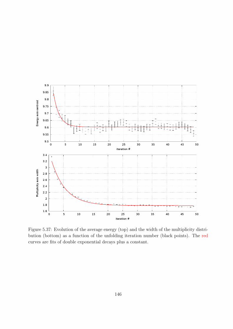
Figure 5.37: Evolution of the average energy (top) and the width of the multiplicity distri-bution (bottom) as a function of the unfolding iteration number (black points). The redcurves are fits of double exponential decays plus a constant.

146

Effect of the prescaling

The initial data distribution can be scaled up (or down) before unfolding. This means inpractice that each point will be unfolded several times. It is a good way to make up for alow statistic and try all the possible unfolded configuration associated with the measured(k,H) distribution.

Figure 5.38: Unfolded distribution with a pre-scaling factor of 1 (left), 50 (center) and 150(right).

Figure 5.38 shows an unfolded distribution for a pre-scaling factor of 1, 50 and 150. Onenotice that the larger the pre-scaling the smoother the final distribution is. It is there-fore important not to scale too much up, for that may smooth out sub-structures in thedistribution. On the opposite side, not enough scaling will lead to important statisticalfluctuations.

There is no rule to choose the pre-scaling factor. The good factor would depend on manyparameters such as the number of iterations, the number of counts in the original distribu-tion, the size of the matrix, the dispersion of points in the distribution, even the responsematrices will influence the need for a pre-scaling. It is generally recommended to get anumber of point in the starting (k, H) distribution of the order of a few thousands. Asan arbitrary rule of thumb, we choose to scale up the input distribution by the size of thematrix (i.e. 32 for a 32-by-32 matrix).

Separation of peaks

We also want to check if and with what precision the unfolding can separate two distinctpeaks, as the distributions we study may have structures.

In practice, neighbouring peaks in a distribution may be fused together in the foldeddistribution because of the loss of resolution and that will lead to the two peaks beingunresolved or connected in the unfolded distribution. More iterations will be needed to

147

get a separation, and the shape of the peaks will be incorrectly reproduced. Figure 5.39and 5.40 show different examples for two peaks distributions.

In general, we conclude that the unfolding procedure fails to reproduce sub-structures fornot clearly separated peaks. Peaks that are too close together are distorted and theirrelative intensity is not conserved in the unfolding. Therefore, we should regard all visiblesub-structure as possible artefact and be careful in the interpretation of the shape ofthe distribution: only the average quantities (centroid, widths, possible tilts, ...) can beconsidered certain.

148

Figure 5.39: Source (top), folded (middle) and unfolded (bottom) distributions for twopeaks, with the peak at lower multiplicity having less counts. The separation between thepeaks is still visible in the unfolded distribution, but they are distorted and their relativeintensity has changed.

149

Figure 5.40: Source (top), folded (middle) and unfolded (bottom) distributions for twopeaks. The separation is good in the source distribution, but are deformed in the unfoldeddistribution.

150

Macroscopic quantities

It is possible to determine the goodness of the unfolding by inspection of global parametersof the distribution: mean value, widths, position of the maximum, shape, ... In particular,we can verify the agreement between the original (k, H) distribution and the refolded matrixfrom the unfolded result. Figure 5.41 shows the evolution of the average multiplicity ofthe refolded distribution as a function of the iteration number and how it compares to thesource (k, H).

Figure 5.41: Average multiplicity of the refolded distribution (black points) compared tothe original (k, H) distribution (red points) as a function of the iteration number. The twoquantities agree for iteration above ≈ 8.

χ2 between distribution

We can compare two distributions precisely using a measurement of the difference be-tween the two. For two distributions N (1)(M, E) and N (2)(M, E), we calculate χ2 =

M,E

N (2)(M, E) − N (1)(M, E)2

; χ2 is zero for equal distributions and positive for differ-

ent distributions.

First, the difference between a test (M, E) distribution (as in 5.31) and the unfold of thefolded source has been measured as a function of the iteration number on figure 5.42: theχ2 drops for the first ≈ 10 iterations, is minimal for ≈ 12− 15 iterations and grows again.This suggest that the best unfolding result is obtained for a number of iteration between10 and 15.For the experimental distribution, we don’t have a distribution to compare the unfolded

151

response to, but it is possible to compare the source (k, H) distribution to a refold of theunfolded distribution, and compare the two distribution. Figure 5.43 shows the evolution ofχ2 with iteration number. The differences between the distributions decrease exponentiallyover the ≈ 10 first iterations. Contrary to the test distribution, the χ2 does not grow athigh iteration number but is rather stable. This confirms that at least ≈ 10 iterations arenecessary to get a proper unfolding and that additional iteration above ≈ 20 are at bestnot useful (figure 5.43), and possibly harmful (figure 5.42).

Figure 5.42: χ2 of the source (test) and unfolded distribution as a function of the iterationnumber. The red line is an exponential decay plus a linear function fitted on the data(black points).

Figure 5.43: χ2 : difference between the experimental (k,H) distribution and the refoldedunfolded distribution, as a function of iteration number. The χ2 stabilises above niteration ≈15. The red line is a double exponential decay fitted on the data. Note the log scale in χ2.

152

Choice of parameters

As we showed, the choice of unfolding parameters is of importance: too much smoothing(via a large pre-scaling) will hide possible sub-structures, while not enough statistics ortoo many iterations may create artefacts from statistical fluctuations. The good set ofparameters depends on the entrance distribution, the size of the matrices, the precisionof the response, ... it is therefore hard to fix one good set of parameters to perform theunfolding.

Based on the test of the unfolding procedure, we find that the optimum parameters are:about 20 iterations and a pre-scaling factor of the order of 30. But to account for thepossible artefacts and consider only the persistent features in the unfolded distribution,we will scan over several set of parameters and consider only the characteristics of theunfolded distribution that are independent of the unfolding parameters.

5.10 Experimental Calorimetric measurements

5.10.1 (k,H) distribution

For 254No, we obtained the calorimetric distributions of fold and observed energy : (k, H),at the two beam energies. We isolated in particular the recoil-gated (k,H) distributionand the recoil-α-gated (k,H) distribution. Figure 5.44 shows the (k, H) distributions forEBeam = 219 and 223 MeV, the recoil-α-gated distributions are shown on figure 5.45. Theisomer-gated distributions are on figure 5.46. To obtain these distributions, the selectionis done on ∆Timplant - decay and EDecay in the DSSD, see figure 5.23. They have only about30 counts in total, while up to 300 were expected. The high thresholds in the DSSD andthe issue with correlation explains the poor statistic for isomer events. The unfolding ofthose events will likely not be relevant, due to the low number of counts.

In figure 5.44 we see that some events have a significant contribution at (0, 0), whichcorrespond to a recoil being detected at the focal plane of the FMA but no γ-ray is de-tected in Gammasphere; those events account for about 6 % of the population. In bothfigures 5.44 and 5.45, we also observe events with larger high (k, H) which correspond toevent contaminated by random γ-rays, those events, correspond to about 3 % of the totaldistribution, in agreement with the rate of random γ-rays.

153

Figure 5.44: Recoil gated (k,H) distributions for EBeam = 219 (left) and 223 MeV (right).

Figure 5.45: Recoil-α gated (k,H) distributions for EBeam = 219 (left) and 223 MeV (right).

154

5.10.2 Unfolding

The (k,H) distributions are afterward unfolded using the responses as described earlier (seesection 5.9). Figure 5.47 shows an example of an unfolded distribution (M, E), compared tothe original (k,H) distribution; plus the refold of the result, in order to check at the foldingof the obtained (M, E) distribution reproduces the experimental (k, H). The unfoldinggives the multiplicity and sum energy distribution (M,E): the number of γ-rays emitted bythe nucleus and the total energy carried by those γ-rays.

5.10.3 Multiplicity to Spin and ESum to E∗ conversion

The conversion from Multiplicity and Esum to spin and excitation energy is based on generalhypothesises on the formation and γ decay process in the excited nucleus. Figure 5.48 showsthe general picture of the γ decay process. The nucleus is supposed to be formed at anexcitation energy above the yrast line. It decays first by emitting statistical γ that carryan important energy (of the order of 1 MeV) and a small angular momentum (≈ 0.5 );afterward, the γ decay connects with the yrast line or close to yrast bands, and follow itby emitting yrast γs with smaller energy (≈ 200− 600 keV and larger angular momentum(2 per γ).

From this model of γ decay, we can separate the multiplicity in two : the statisticaland yrast multiplicities; such as M = nstat + nyrast. From what we described of theangular momentum for each type of γ decay, we can assert the spin of the original stateas I = nyrast × ∆Iyrast + nstat × ∆Istat. In practice, we cannot differentiate between yrastand statistical decays, that is why we will use an average value for nstat. This lead toI = ∆Iyrast × (M − nstat) + ∆Istat × nstat. The yrast γ-rays are identified as E2 transition,therefore ∆Iyrast = 2 .

Statistical γ-rays

The number of statistical γ-rays nstat is extracted from the γ-ray spectrum. The high energypart of the spectrum is consider the range where only statistical gamma-rays are detected.Therefore a function describing such γ-rays can be fitted and extrapolated. Comparing theintegral of the statistical spectrum to the area of a known transition„ one can extract theratio number of statistical γ-rays per de-excitation cascade in the nuclei [104,105]. We didthe calculations on a high statistic spectrum from Jurogam [31, 106]. The spectrum wasunfolded to remove the Compton contribution and efficiency corrected. We determined

155

Figure 5.46: Isomer gated (k,H) distributions for EBeam = 219 (left) and 223 MeV (right).

Figure 5.47: Example of unfolded experimental distribution. The original (k,H) distribu-tion is on the left, the unfolded (M,E) distribution is in the centre, a refold of (M, E) ison the right and clearly similar in shape to the original (k, H). The distribution unfoldedwas the recoil gated (k,H) for EBeam = 219 MeV, unfolded with the response from 88Y.

156

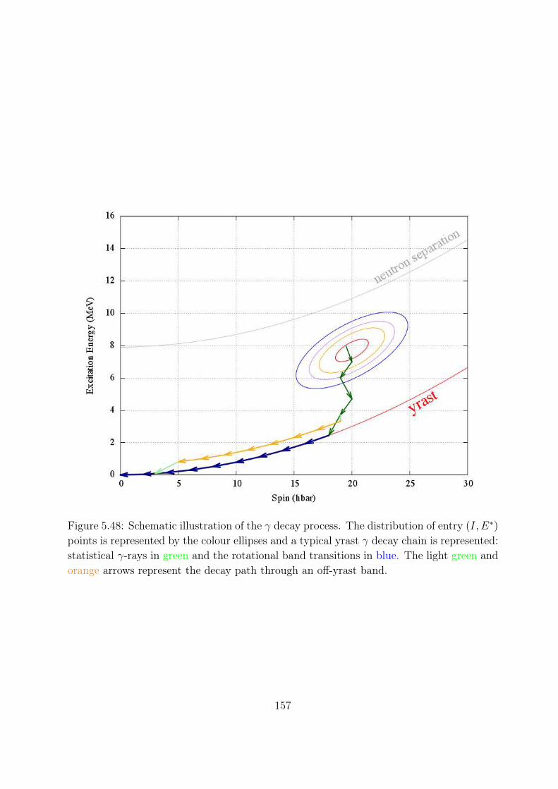
Figure 5.48: Schematic illustration of the γ decay process. The distribution of entry (I, E∗)

points is represented by the colour ellipses and a typical yrast γ decay chain is represented:statistical γ-rays in green and the rotational band transitions in blue. The light green andorange arrows represent the decay path through an off-yrast band.

157

that 2.4 ≤ nstat ≤ 5.9 depending on the shape of the statistical spectrum. The higherbound contains non-statistical events and so the actual number of statistical gamma-raysis expected to be much lower than 5.9. Previous experimental measurement suggestsnstat = 3 [107]. A simple statistical model can be used to check the compatibility of nstat

with the resulting entry distribution.For our experiment, we obtained nstat = 3.0± 0.4. We also assume ∆Istat = 0.25± 0.50 .

Effect of conversion electron

The electron conversion of some transitions, for example at the bottom of the yrast band,means that some γ-rays will not contribute to the observed multiplicity and Esum. Tocorrected for that, we introduce the averages spin and energy carried out by the convertedelectrons: ICE and ECE. The excitation energy and spin are corrected for the conversionelectrons by adding these quantities:

I = ∆Iyrast × (M − Mstat) + ∆Istat × Mstat + ICE (5.3)

E∗ = Esum + ECE (5.4)

The contribution of electrons is calculated according to the known structure of 254No [25,26, 95–97, 108]. The three bands listed are not actually the only bands in 254No, but theycapture most of the γ flux and it is a good approximation to evaluate the contribution ofelectrons. The table 5.8 gives the contribution of the conversion electron in three bands of254No.

Band Population (%) ICE ECE MeVg.s. 44 7.9 0.5948− 30 6 0.8963+ 26 13.6 1.256

Total 100 8.8 0.857

Table 5.8: Table of coefficients for the electron contribution to the energy and spin.

The parameters chosen for the multiplicity to spin transformation are ∆Iyrast = 2 ,∆Istat = 0.25 , nstat = 3.0,ICE = 8.8 and ECE = 857 keV.

158

Effect of isomers

For isomer events, the γ decay as described previously is changed: the decay-path is stuck

in a level at a finite spin and energy. Figure 5.49 shows the decay for an isomer.

Figure 5.49: Schematic illustration of the γ decay process. The distribution of entry (I, E∗)

points is represented by the colour ellipses and a typical γ decay chain leading to an isomeris represented: statistical γ-rays in green and the rotational band transitions in blue. Theγ decay stops at a finite excitation energy and spin.

In that case, the prompt detection of γ-rays will miss all the transitions below the long livedstate in which the decay is stuck. An additional correction is needed for those events: theprevious formulae are modified into: I = ∆Iyrast×(M − nstat)+∆Istat×nstat +ICE +Iisomer

and E∗ = Esum + ECE + Eisomer. One notes that, if not properly corrected with Iisomer andEisomer, isomer events will be assigned to a lower spin and excitation energy in the entrydistribution. This placement will be incorrect, for up to 30 % of events in the case of254No. However they do not affect the region of interest for the determination of the fissionbarrier.

159

5.11 Entry distribution

Following the procedure described above, the (k, H) distributions are unfolded and trans-formed into a (I, E) distribution. Figure 5.50 shows an example of the unfolded (M, E)distribution and the corresponding entry distribution. The points in the entry distributionwill be compared to Eyrast, Sn and E

max (see section 4.1.1), and the evolution of the dis-tribution with spin will be investigated to determine the position of the saddle energy inthe next chapter.

Figure 5.50: (Left) Multiplicity and sum energy distribution (right) and the correspondingentry distribution (spin, excitation energy).

5.11.1 Comparison with previous measurement

The previous measurement by P. Reiter et al. [98] established a lower limit on the fissionbarrier height, via the entry distributions at beam energies of 215 and 219 MeV.

160

Experimental setup

The previous measurement of 254No was also performed with Gammasphere and the FMA,but some details of the experimental setup were significantly different than for the presentexperiment : The number of detector modules was different (101 modules, against 101 fullmodules – Ge and BGO shield – plus 7 modules with only the BGO shield in the presentwork). Moreover, a different set of absorbers were placed before the detectors: Cu andTa (against Cu, Ta and Cd for our work), which increases the detection efficiency at lowenergy ( 200 keV) – in particular, the X-rays will be more efficiently detected. Finally,the trigger mode was different – this prevented the loss due to data falling off the bus –with a Gammasphere trigger requiring nclean Ge ≥ 2. This is a very strong requirement inthe trigger and that will impact the shape of the distribution largely by favouring highermultiplicity and energy.

The response in multiplicity and energy of the previous measurement show clearly a higherdetection efficiency in the original measurement, with a calorimetric efficiency of 70.2 %(63 % for our work). See figure 5.51. The change in efficiency comes not only from thechange in absorbers and trigger mode, but the ageing of the detectors, in particular thephoto-multiplier tubes of the BGOs, is a source of decrease in efficiency. Our responseshave lower resolutions than the previous one, which will affect the unfolded distribution, inparticular this will lead to unresolved sub-structures and larger width of the distributions.

Analysis

At the time of the previous experiment, only the yrast rotational band was known for254No and the electron conversion was considered only for this band in the multiplicity tospin conversion. For those reasons, the published entry distribution in [98] will be overallin agreement with our measurement but not necessarily exactly like it. It is possible tocompare the unfolded (M, E) distributions and check if the data are compatible.

Figure 5.52 compares the (M, E) distribution for EBeam = 219 MeV from [98] and theequivalent distribution from our experiment with a software requirement of 2 clean Ge.No multiplicity to spin conversion has been done. The two distributions have strongsimilarities:

• The energy range is about the same for the two distribution: from ≈ 1.5 − 2 to≈ 10 MeV.

161

• The distribution in multiplicity are very similar: in the 2 to 11 range, with a maximumat ≈ 6.5.

• The average energy of the two distribution are about the same: 5.2 MeV for P.Reiter, 5.3 MeV for our work, and the maximum of the distributions are 5.7 MeVand 6.0 MeV respectively.

• In the original measurement, the average multiplicity is 7 against 6.5 in our work.

In short, for two distributions taken in the same conditions (nclean Ge ≥ 2), the unfolded(M, E) distribution are very similar, indicating the agreement between the two data setand validating the unfolding procedure.

162

Figure 5.51: Comparison of the energy (left) and multiplicity (right) responses for theentry distribution measurement by P. Reiter (blue) and our work (red). The previousmeasurement clearly had a better calorimetric efficiency.

163

Figure 5.52: Comparison of the (M, E) distribution measured in P. Reiter’s experiment(left) and our work (right) : distribution (top), multiplicity projection (middle) and energyprojection (bottom).

164

Chapter 6

Entry distribution and fission barrier of254No

In this chapter, we will examine the entry distribution produced following the proceduresdescribed in sections 5.8, 5.9 and 5.10 and determine the height and spin dependence ofthe fission barrier.

6.1 Entry distribution: measurement and analysis

6.1.1 Measured unfolded distributions

The (k, H) distributions are unfolded and converted to entry distribution according tothe transformation explained earlier – see sections 5.8, 5.9 and 5.10. Figures 6.1 and 6.2show the entry distributions for recoils, α and isomer-gated events. As mentioned insection 5.9.3, we will analyse the results of several unfoldings for each (k, H) distribution,with iteration numbers between 10 and 20 and different scalings; this to avoid any artefactthat a particular set of unfolding parameter could create.

Contribution of the isomers to the entry distribution

In the recoil-gated distribution, the isomeric events are unfolded using the same parametersas for the general distribution. This is technically incorrect: γ cascades feeding isomericstates will yield a lower value of spin and excitation energy, since the isomer decays outside

165

Figure 6.1: Entry distributions for EBeam = 219 MeV (left) and 223 MeV (right) for recoil-gated events, unfolded with 88Y statistically built response. The yrast line is drawn in red,the neutron separation is the dotted line in gray and the range of maximum excitationenergy is marked with two dotted blue lines. For each spin bin, the point of half maximumE1/2 is marked.

166

of Gammasphere (at the FMA focal plane). The isomer-gated entry distributions allowus to determine where on the (I, E∗) distribution the isomer events lie – figure 6.3. Theisomer-gated distributions show that the associated events sit at low energy (≈ 2−4 MeV)and spin (≈ 5 − 17 ). Below the average of the recoil or α-gated distribution. Therefore,γ cascades populating the isomers contribute to the entry distribution at artificially lowspin and excitation energy, and will not modify its profile at high (I, E∗), which is wherewe expect to see effects of the fission barrier. However, the average and maximum of thedistribution could be shifted down by those events. But we will see that the isomer effectis small in the spin range of interest for our measurement.

6.1.2 Analysis of the Entry Distribution

To analyse and qualitatively compare the entry distributions, we need to choose specificobservables to look at and be able to quantitatively compare different distribution. Wechoose values that give information on the shape of the distribution and how it extends.

Global quantities

We first consider quantities that are global :

Position of the maximum: The first quantities of interest is the point with maximumpopulation: (I, E∗)max.

Average Spin and Energy: The projections on the I and E∗ axes lead to an average spinand excitation energy that is, a priori, different from the position of the maximum.

Width and asymmetry of the distribution: Finally, the distribution extends in thespin and excitation energy in a certain way, characterised by the width of the pro-jected distribution and the asymmetry (measured with the skewness, which is theratio of the third moment of the distribution over the cube of the standard devia-tion).

These global quantities are basic and simple to extract but give us very valuable informationon the distribution. Table 6.1 gives these values for the recoil-gated distributions. We seethat increasing the beam energy increases the average spin by 2.5 and changes the positionof the maximum spin from 13 to 19 . The average energy is increased by 1 MeV, the

167

Figure 6.2: Entry distributions for EBeam = 219 MeV (left) and 223 MeV (right) for α-gatedevents, unfolded with 88Y statistically built response. The distribution at EBeam = 219 MeVhas only 51 % of the statistics at EBeam = 223 MeV.

Figure 6.3: “Entry distributions” for EBeam = 219 MeV (left) and 223 MeV (right) forisomer-gated events, unfolded with 88Y statistically built response. The very low statisticof isomer events makes it difficult to interpret the entry distribution, but demonstratesthat they are artificially shifted in spin and energy.

168

EBeam (MeV) 219 223(I, E∗)max (13 ± 0.31, 3.1 ± 0.2) (19.3 ± 0.7, 6.3 ± 0.5)

Average spin () 15.9 ± 0.6 18.3 ± 0.7

Spin width () 4.0 ± 0.2 4.17 ± 0.1

Spin Skewness 0.25 ± 0.1 0.0 ± 0.1

Average energy (MeV) 5.2 ± 0.1 6.2 ± 0.2

Energy width (MeV) 2.7 ± 0.1 3.1 ± 0.1

Energy Skewness (MeV) 1.2 ± 0.3 0.8 ± 0.1

Table 6.1: Global characteristics of the recoil-gated entry distribution. The values areaverage over several unfold with 88Y response and different number of unfolding iterationsand pre-scaling factor. The error bars reflects the dispersion of values for different unfolds.

maximum energy is up by 3 MeV. Furthermore, the distribution gets more symmetric athigher beam energy.

α-gated events show the same behaviour for the average values, but the maximum pointdoes not change and the shape of the distribution is very different. The change in shapecan be explained in part by the better selectivity of the α-tagging (rejection of possiblecontamination) and mostly low statistics (The α-gated distribution have 60 % less statisticsthan the recoil-gated ones, see section 5.6.2). Table 6.2 give the values for α-gated entrydistributions.

EBeam (MeV) 219 223(I, E∗)max (18.7 ± 0.9, 6.2 ± 0.8) (19 ± 1, 5.9 ± 0.3)

Average spin () 16.4 ± 0.1 19.2 ± 0.1

Spin width () 4.3 ± 0.2 4.9 ± 0.1

Spin Skewness −0.1 ± 0.2 −0.1 ± 0.1

Average energy (MeV) 5 ± 0.1 6.5 ± 0.1

Energy width (MeV) 2.2 ± 0.1 3.5 ± 0.1

Energy Skewness (MeV) 0.7 ± 0.3 0.9 ± 0.1

Table 6.2: Global characteristics of the α-gated entry distribution.

Spin dependent quantities

In addition to the global characteristics of the distribution, we are particularly interestedin the spin dependence of the energy distribution. For this purpose, we will look at the

169

projection on the excitation energy axis for each spin slice (the spin slices are 2 widebecause of the multiplicity to spin transformation that multiplies M by 2). For each spinslices, we will look at similar quantities: average excitation energy, distribution width, ...

Evolution of spin population As hinted from the average and width of the spin dis-tribution, the spin increases with beam energy: the average spin is higher at higher beamenergy. However, the comparison of the spin population on figure 6.4 shows that the twospin population both fall to 1/10 of the maximum above spin 26 . This behaviour is

Figure 6.4: Spin distribution profile for EBeam = 219 MeV recoil gated (blue) andEBeam = 223 MeV recoil gated (red). The blue and red arrows mark the spins for whichthe distribution at EBeam = 219 and 223 MeV falls to 10 % of the maximum.

an indication that a limit is reached in 254No since adding more energy in the reactionincreases the average spin, but does not increase the maximum spin by much.

Half maximum points A key quantity we are examining is the half maximum energyE1/2, i.e. the energy at which the distribution falls below half of its maximum. In particular,we are looking above the maximum of the distribution – the way to determine this energyis described in appendix F. In previous measurements, the E1/2 points have been used asestimates of the fission barrier height [71,98] – or at least a lower limit.

We will also consider Emax, the energy with the maximum population at each spin. Fig-ure 6.5 shows the energy distributions at spin 20 for the recoil-gated entry distributionsat EBeam =219 and 223 MeV.

170

Saturation of energy with spin In the plots of E1/2 and Emax as a function of spin,we observe a saturation of these quantities at high spins – see figures 6.6 and 6.7. For spins17 to 23 there is a clear saturation of E1/2 ≈ 8 MeV and Emax ≈ 6 MeV, which is visiblein the recoil and α-gated distributions.This is a clear indication that although the increased beam energy makes possible a largerexcitation energy in the nucleus, the excitation energy is limited. This saturation is at-tributed to fission: with E∗ getting closer to ESaddle, the fission width becomes importantand reduces the γ-decay probability Pγ = Γγ/ (Γγ + Γfission).

Below spin ≈ 15 , the E1/2 points do not have a trend following the saddle energy. Thiscan be explain by several factors: The entry distribution could be artificially shifted downto lower excitation energy by isomer events, as suggested by figure 6.3. The lowest spindistribution could be depleted by the 3 neutron evaporation channel. Finally, in the excitednucleus, at low spin, the E∗ − Erot(I) is larger which translates into a larger temperatureT , therefore the neutrons emitted by the 255No∗ at low spins to form 254No will removemore kinematic energy following < Kneutron >∝ T [109].

For spins 25 , we do not consider the E1/2 or Emax points relevant as less than 5 % ofthe total population is above spin 25 , the width of the energy distribution increases upto 4 MeV, larger than the response width (≈ 2 MeV) and the values are not independenton the unfolding (in particular in figure 6.7). Moreover, these points originate from theevents suffering from random summing in the (k, H) distributions. The behaviour of thosepoints is likely a pure effect of low statistics in the tail of the distribution and randomeffects in the unfolding.

171

Figure 6.5: Energy distribution at spin 20 for the recoil-gated entry distributions atEBeam =219 (blue) and 223 MeV (red). The E1/2 and Emax points of the distributions aremarked. The Emax values are the same for the two beam energies (7 MeV), the E1/2 valuesdiffer(8 and 9 MeV). The blue and red arrows mark the energies for which the distributionat EBeam = 219 and 223 MeV falls to 10 % of the maximum.

172

Figure 6.6: Saturation of the E1/2 (purple) and Emax (green) with spin for EBeam (Top)219 MeV (Bottom) 223 MeV in recoil-gated distributions. The yrast line is shown in redand the neutron separation energy in gray. Points are gathered from different unfolds anddispersed around the corresponding spin for better visibility.

173

Figure 6.7: Saturation of the E1/2 (purple) and Emax (green) with spin for α-gated distri-bution at EBeam (Top) 219 MeV (Bottom) 223 MeV. The yrast line is shown in red and theneutron separation energy in gray. Like in figure 6.6, the energies saturates at respectively8 and 6 MeV from spin 14 to ≈ 24 .

174

6.2 Extraction of the saddle energy

From the experimental data, it is possible to extract the value of Esaddle, which can indi-rectly give the height of the fission barrier Bf = Esaddle − Eyrast; in particular, at spin 0,Bf (0) = Esaddle(0) .

6.2.1 Fit on E1/2

We assume that the experimental E1/2 points in the distribution correspond to the the-oretical E1/2 points (see section 3.2.5) for which Pγ(E1/2) = 0.5. Therefore, using thecalculated relation ∆(I) = E1/2(I) − Esaddle(I), we can deduce the height of the saddleenergy and its spin dependence.

We will fit the saddle parametrization Esaddle = Bf (0) + I(I+1)2Jsaddle

(see also equation 2.6)on the experimental E1/2 − ∆(I) points, with ∆(I) chosen from the ones calculated inchapter 3. We restrict the fit to the points where a saturation of E1/2(I) is observedbecause it is the only range where we expected a direct relation between E1/2 and ESaddle.This means the behaviour of ESaddle at lower spins and in particular the value of Bf (0) willbe extrapolation. Figure 6.8 shows the fit on recoil-gated data.

We found Bf (0) = 6.2± 0.8 MeV, in good agreement with macroscopic-microscopic modelcalculation (6.76 MeV [1, 2]) and JSaddle = 145 ± 60

2/MeV for the saddle moment ofinertia, just between the rigid body value (180.7

2/MeV) and the value calculated in theHFB framework (140

2/MeV) or the scaled SD band moment of inertia (142 2/MeV, see

section 3.1). We note that the value of JSaddle is the same for all spins. Table 6.3 gives theresults of the fit on different data set (beam energies and α-gated) as well as the averagevalue.

6.2.2 Mapping the best parameters

We propose to visualise what parameters for the saddle energy Bf (I = 0) and Jsaddle

are compatible with our experimental data. We establish a measure of the compatibilitywith the experimental data and E

Bf (0),Jsaddle

saddle : χ2 is defined in 6.1 as the squared differencebetween our experimental Esaddle = E1/2 − ∆(I) and a calculated E

Bf (0),Jsaddle

saddle .

χ2 =n

0

E(n)1/2 − ∆(I(n))

− EBf (0),Jsaddle

saddle (I(n))2

(6.1)

175

Figure 6.8: Fit of the E1/2 −∆ ≈ Esaddle experimental data point for recoil gated events atEBeam = 219 MeV (top) and 223 MeV (bottom). The yrast line is represented in red andthe neutron separation threshold in gray. The data points (from several unfolding results)are in blue, the thick black line is the fitted Esaddle, for which the parameters are given intable 6.3.

176

Data set Bf (0) (MeV) MoI (2/MeV )Ebeam = 219 MeV 5.41 ± 0.5 66 ± 25

Ebeam = 219 MeV, α gated 5.7 ± 0.6 113 ± 35

Ebeam = 223 MeV 6.8 ± 0.5 179 ± 25

Ebeam = 223 MeV, α gated 5.7 ± 0.5 147 ± 40

All data combined 6.6 ± 0.6 183 ± 35

Average 6.2 ± 0.8 145 ± 60

Table 6.3: Results of the fit on E1/2 −∆(I) data, to extract the saddle height and momentof inertia. All data combined is a fit done on all the data. The average values are averageon the fit results, weight by the uncertainties and the number of events for each data set.

When scanning over all the possible Bf (I = 0) and Jsaddle, the regions of lowest χ2 are themost likely parameters for the saddle. Figure 6.9 shows the map of χ2 values and comparesit with predictions and our experimental measurement.

One notes that this method is just a visualisation of the fit procedure and does not bringnew information. But it clearly shows why the uncertainty on Bf (0) is rather small whilethe uncertainty on the moment of inertia is important: this is linked to the topology of theχ2 surface.

177

Figure 6.9: Map of χ2 value calculated for all the data points in our experiment. Themoment of inertia of the yrast line is marked in red, the predictions for moment of inertia(by HFB or scaled SD, see 3.1) is in purple, the rigid body moment if inertia is in orange.The neutron separation energy is in black, the predicted Bf (0) by Macroscopic-Microscopiccalculations is in blue, and the value from HFB calculations in purple (see 3.1). The valuesfrom the fit and the uncertainties are represented with the black ellipse.

178

6.3 Conclusions on the Fission barrier

The fit on E1/2 give a saddle parametrization with Bf (0) = 6.2 ± 0.8 MeV and Jsaddle =

145 ± 60 2/MeV, in agreement with predictions. Our result favours the fission barrier

height calculated by microscopic-macroscopic model and the measured moment of inertiais between the HFB result and the rigid body values – see section 3.1. Figure 6.10 shows

Figure 6.10: Plot of the fission barrier spin dependence. The two external thin linescorrespond to the limits and the thick line is the average. Bf (I) stays sizeable up to spin30 , but could drop below 2 MeV above 30 . The uncertainty on Bf is lower betweenI = 15 and 20 since the fit was performed on this region.

the height of the fission barrier as a function of spin. It is in agreement with previousmeasurement [98] with Bf (20) = 4.8 ± 0.5 MeV and stays sizeable up to spin 30 .

6.3.1 Agreement with ∆(I)

As mentioned in chapter 3, the ∆(I) is a calculated quantity dependent both on thesaddle energy and the model used for the calculation. However, the effect will be lessdramatic since we are considering points around spin 15 to 20 where ∆(I) is smallerand the different models agree better – see figure 3.2.5. We tried different height and spindependence of ∆(I) and extracted the saddle energy each time and found that the variationof Bf (0) is less than 0.1 MeV and and the variation of JSaddle is less than 5

2/MeV. Thisweak dependence on ∆ is explained by the uncertainties on E1/2 and the dispersion of thepoints on which the fit is done. In the end, the dependence on ∆ is shadowed by other

179

uncertainties.

6.3.2 Agreement with calculation

There is a general agreement with the calculations for the global quantities. Although theaverage spins do not agree in absolute values but the ≈ 2.5 increase between EBeam = 219

and 223 MeV is consistent with what was seen in calculation. For the energies, the 5 and6 MeV average and ≈ 1 MeV increase between the two beam energies is consistent with thecalculations. Although the details of the shape of the calculated distributions were some-what different from the experimental measurement, as visible on figure 6.11, there is ageneral agreement within our experimental uncertainty. This allows us to validate our con-clusion and affirm that the saddle energy in 254No is determined by Bf (0) = 6.2± 0.8 MeVand a moment of inertia Jsaddle = 145 ± 60

2/MeV.

We successfully performed the first experimental measurement of a fission bar-

rier in the Transfermium region.

180

Figure 6.11: Comparison of the experimental (top) and calculated with KEWPIE2 (bot-tom) entry distribution for 254No at Ebeam = 219 (left) and 223 MeV (right).

181

182

Chapter 7

Perspectives

7.1 Measurement improvement: digital electronics

The main limitation in our experiment is the limited amount of statistics. This is due inpart to the beam intensity kept down to keep the count rate in Gammasphere at ≈ 10 kHz,below the acceptable limit. It is also due to the FMA poor transmission.

The move from analog to digital electronic for detectors will reduce the dead time in dataacquisition and allow the use of higher intensities on target (Jurogam in Jyväskylä accepts arate up to 40 khz). For small cross-section, this will easily bring a 2 to 4 gain in productionrate. This offer to the experimentalist options to perform experiment faster or collect morestatistics or explore regions of the nuclear landscape where production cross sections aresmaller. See appendix B.1.

The Argonne Gas Filled Analyzer (AGFA) project at Argonne National Laboratory willbe a high transmission separator for such studies.

7.2 Neutron effect

In this analysis, we did not take into account the effect of neutrons in the (k, H) distribution.Indeed, two neutrons are emitted in coincidence with the 254No γ-rays and interact withthe environment and the Gammasphere detectors: we see γ-rays energy from neutronscattering on Ge in the prompt spectra, proving that neutrons contribute to the fold andmeasured energy. The question is: how much is the (k,H) distribution affected by neutrons?

183

We have started running GEANT4 simulation of neutron in Gammasphere, including de-tectors thresholds, data loss, ... The simulated γ efficiency is in agreement with experi-mental measurements. Simulation of the response to neutrons is underway, but one needsto be careful especially since GEANT4 has some trouble with neutron scattering at lowenergy [110].

The effect of neutron is believed to be small enough so that the bulk of the distribution isnot changed significantly and the changes are expected to be smaller than the differencesin (k, H) distribution observed at the two beam energies. See appendix A for more details.

7.3 Complementary measurements

7.3.1 Prompt electron spectroscopy

The prompt spectroscopy of conversion electrons in 254No performed with the SACREDarray confirmed the ground state rotational band low spin levels. This experiment alsohighlighted the conversion of electrons from high-K bands [111].

A proposal for “Study of high-K states in 254No using the SAGE spectrometer” has beenaccepted at JYFL and will yield extra information on the electrons from high-K bands. Aswe saw in the data analysis, a good understanding of the electron conversion is necessary tocorrectly reconstruct the entry distribution. The configuration of identified and expectedbands lead to large M1 admixtures in ∆I = 1 intraband transitions, which are highlyconverted (section 5.10.3).

7.3.2 Formation of 254No by other reactions

A measurement of the entry distribution of 254No produced in a different reaction wouldbe a good way to test our results. In addition, 254No formed in, for example, the hot fusionreaction 238U (22Ne, 6n) will likely be populated in a different region of spin (and maybeexcitation energy). Exploration of a different spin range would be a good way to confirmthe extrapolated values of Bf (0).

184

7.3.3 Measure of partial fusion cross section

As mentioned in chapter 2, the sub-processes in fusion-evaporation reactions are still mostlyunknown and could influence the final spin (and energy) distribution of the evaporationresidues.

The current experimental measurements of such fusion cross section are scarce and focusmostly on energies above the fusion barrier [112,113]. More measurement around the bar-rier would give valuable information on the barrier distribution, validate coupled-channelcalculations and lead to better simulation of the compound nucleus spin and energy dis-tribution.

7.3.4 Improvement of cascade code and simulations

Following the previous point, there is no code today that can calculate from the compoundnucleus to the evaporation residue and provide an entry distribution. We started creatingsuch codes with our modifications of KEWPIE2 and the cascade code using NRV data. Afully integrated code that would compute cross sections and entry distributions, with thepossibility of changing the saddle energy or entrance spin distribution according to differentmodels, would be very helpful to interpret entry distribution data. Moreover, coupling suchcode to a γ-decay cascade calculation and the GEANT4 simulation of Gammasphere thathas been developed for this work would give a full simulation framework for such studies.

7.3.5 Systematic spin measurement in other facilities

In order to build a systematic of measurements over a wide range of excitation energiesand nuclei, it might be possible to collect fold information and reconstruct the entry spindistribution.

For any detector array registering γ-rays in Ge and anti-Compton shields, it is possibleto get a fold measurement and a proper fold response calibration. Realistic simulationsfor the Jurogam array suggest a multiplicity response as in figure 7.1. The detectionefficiency is clearly much smaller than for Gammasphere (of the order of 25 %), but for γ

multiplicity above 5, it will be possible to extract a correct average entry spin. Moreover,the high transmission of a separator like RITU would bring high statistics data. This hasto be confirmed by more developed calculations (for example within GEANT4) and sourcemeasurement to build an actual response.

185

Figure 7.1: Simulation of the multiplicity response in a multi-Ge detector like Jurogam.The detection efficiency is poor but still enough for multiplicities above 5.

186

7.3.6 Measurement of 255Lr entry distribution

Following our measurement of 255No fission barrier, we proposed to measure the samequantity for 255Lr. This measurement in an odd-A nucleus will provide information on therole of the odd nucleon, on the K quantum number and the reduced pairing. In addition,investigating the evolution of the fission barrier for increasing Z, is a natural next step.The proposal has been approved by the ATLAS PAC.

For 255Lr, Möller et al. [1] predicts a barrier height of 6.6 MeV. This is close to the 255Novalue and that makes it a good case for comparison. Moreover, it is expected that the oddnucleon will increase the stability of the nucleus and an experimental measurement of thiseffect is of great interest [114].

We already ran theoretical calculations for the proposed reaction in order to assess thepossible observations – see figure 7.2. We expect the same competition between γ andfission decay than for 254No and it is very likely that it will be possible to extract a fissionbarrier value from the experiment. Moreover, the upgrade of Gammasphere to digitalelectronic will help us by allowing a more intense beam on target and greater statistics bya factor 3 to 5.

7.3.7 Insight on the reaction mechanism from the entry distribu-

tion

The entry distribution is primarily sensitive to the position of the saddle, but it can alsogive some insights on the whole reaction mechanism. It is possible to extract the averageenergy removed by the neutrons emitted by the compound nucleus following E = ECN −S2n − Kn1

− Kn2. The low population of low spins may be a consequence of depletion

of those partial waves in the reaction mechanism. More work on the entry distributionand theoretical interpretation is needed to decelerate between reaction mechanism andexperimental effects.

187

Figure 7.2: Theoretical calculations of an entry distribution for 255Lr in the reaction209Bi(48Ca, 2n) using KEWPIE2 [8,80]. The yellow represent the excitation energy wherethe widths for γ and fission decay are approximately equal.

188

Appendix A

Effect of neutrons

In the fusion-evaporation reaction used to populate 254No, two neutrons are ejected fromthe compound nucleus and carry energy. Those neutrons may interact with the Gamma-sphere detectors, deposit energy and register hits. This cannot be removed in the dataanalysis since the neutron hits are obviously coincident with the 254No γ-rays. Therefore,a correction of the neutron contribution has to be applied in the (k, H) distribution beforeunfolding.

A.1 GEANT4 Simulation of the neutron contribution

The response of Gammasphere to neutrons with a Maxwellian distribution of kinetic ener-gies with < E >= 2 MeV has been simulated with GEANT4 [115]. The neutron inducedsignals are qualitatively well reproduced by the simulation, as shown on figure A.1. Butwe still have to verify the absolute intensity of the neutron contribution.

The average energy deposited in Gammasphere by one neutron of energy 2 MeV is Hneutron ≈560 keV and the average fold is kneutron ≈ 1.0. Figure A.2 shows the energy and fold re-sponse for one-2 MeV neutron.

189

Figure A.1: Overlay of an experimental and simulated neutron induced spectra. In black,the experimental spectrum (from [116]), in blue the simulated spectrum. The γ-ray energiesmarked in orange are the ones not seen in experiment because of the time cut and detectionthresholds. The energies marked in red correspond to the materials not included in theGEANT4 simulation because our experiment did not use hevimet shields (see section 4.1.6).

190

Figure A.2: (Top) Gammasphere response in energy and fold to neutrons with a Maxwelliandistribution of energy and < Eneutron >= 2 MeV. The distribution does not show the (0, 0)point with 37 % of the population. (Bottom) Distribution of fold from neutrons with aMaxwellian distribution of energy and < Eneutron >= 2 MeV.

191

A.2 Correction of the neutron contribution

The neutron contribution is statistically removed from the measured (k,H) distribution,taking into account that k and H need to stay positive. The correction for 2 MeV neutronsreduces the average fold by 28 % and the average energy measured by 16 %. Figure A.3shows the (k,H) distribution before and after correction for the neutrons. The averageneutron correction applied is 1.1 for the fold (up to 5) and 550 keV (up to 4 MeV). Usinga Maxwellian distribution for the neutron energies reduces the neutron fold contributionby 15 %.

Figure A.3: (k,H) distribution without (left) and after (right) neutron contribution removal.Although the bulk of the distribution is not changed, the slope is slightly shifted up andthe distribution is denser at lower folds.

A.3 Caveat

The GEANT4 simulation is doing a good job at reproducing the gamma-ray efficiency(simulation finds a calorimetric efficiency of 63 %) - but further work is required to test theneutron response. There is a known issue in GEANT4 that low-energy neutron inelastic

192

scattering is not correctly reproduced (cross sections, angular distributions and energyof recoils and neutrons, gamma lines...) [110]. Until all the issues are resolved, it is notjudicious to attempt a correction of the neutron effects.

Another issue is that we do not know what the kinetic energy distribution of the neutrons,the kinetic energies of the neutron evaporated by 256No and 255No being probably different.The measured entry distribution can give indication on the sum energy spectrum of thetwo emitted neutrons.

193

194

Appendix B

New and upgraded facilities for the

study of SHN

B.1 Digital Gammasphere and FMA

Gammasphere suffers from some technical limitations: The Germanium signal shapingtime is ≈ 10µsec, which leads quickly to pile-up as the count rate increases (40% pile-upat 50kHz). Moreover, the acquisition dead-time is of the order of 25µsec per event, hencea one- or two-fold γ trigger saturates the DAQ capabilities.

To allow higher beam intensity on target, increased rates and a more flexible trigger,Gammasphere is being upgraded with digital electronic1. This will reduce the shapingtime down to 2µsec and enable the observation of γ-rays with rates as high as 40 kHz(compared to 10kHz now). In addition, the FMA electronic is also being upgraded withdigital electronic.

B.2 Gretina

GRETINA is the first phase of an American project of γ-ray tracking detector calledGRETA (Gamma Ray Energy Tracking Array) [117]. This detectors use pulse shapeanalysis in a large highly-segmented Germanium crystal to determine the interaction point

1The digital electronic used in Digital Gammasphere is the same as the one designed for Gretina. See

B.2

195

of the γ-ray in the crystal. Moreover, this type of detector does not use BGO shield tosuppress Compton scattering, but uses a full array of Germanium crystals and tracking isperformed to reconstruct scattering events.

The Gretina array is under commissioning at the Berkeley Gas Separator at Berkeley andhas been tested mainly on the 208Pb (48Ca, 2n)

254 No reaction.

A similar tracking array is under development in Europe under the name AGATA (Ad-vanced GAmma Tracking Array) [118]. AGATA has not been used in V&SHN reactionsyet, but a V&SHE study program is schedule with the Exogam and the VAMOS separatorwhen AGATA will be installed at GANIL.

B.3 Jurogam, Ritu, GREAT

The University of Jyväskylä hosts a very efficient setup for the study of V&SHN.

Jurogam is a γ-ray multi-detector array composed of 39 Germanium detectors – 24clovers and 15 mono-crystals – Compton suppressed with BGO shields. The detectionefficiency is 6% at 1.33 MeV.

Digital electronics have recently been installed on Jurogam, allowing an energy resolutionaround 2.6% at 1.33 MeV even at count rates as high as 70 kHz in one clover detector.

RITU The Recoil Ion Transport Unit (RITU) is a gas-filled magnetic separator. Itis composed of a quadrupole, a magnetic dipole for separation and a horizontal-verticalquadrupole doublet for focusing. In a gas filled separator, the recoil charge state is the re-sult of an electron exchange equilibrium in the gas and depends only on the atomic chargeand the recoil velocity ; hence the recoils are separated according to an average charge state.

RITU’s transmission is between 2 and 35% depending on the recoil. The overall lengthof the separator is only 4.8m, and that favours the study of short lived isomers with thereduced flight time.

GREAT The focal plane detection system GREAT (Gamma Recoil Electron Alpha Tag-ging) is used to identify the recoils and perform decay spectroscopy. It is composed of one

196

Figure B.1: Jurogam, RITU, GREAT facility at the University of Jyväskylä.

197

Multi-wire proportional counter for energy loss, time of flight and focal plane positionmeasurements, one DSSD to implant the recoils and observe subsequent electrons and α

decays, one Silicon tunnel to measure escape electrons and αs, one segmented planar Gedetector for detection of low energy γ-rays and X-rays correlated with the DSSD pixels,and BGO suppressed clover Ge detectors to detect γ rays.

SAGE The Silicon And GErmanium (SAGE) spectrometer combines the Jurogam γ

detectors and an electron detection system. This spectrometer aims to measure convertedelectrons at the target position, for the spectroscopy of highly converted transition inV&SHN.

B.4 JINR

The Flerov Laboratory for Nuclear Reaction, at the Joint Institute for Nuclear Research inDubna, Russia, hosts the GABRIELA spectrometer, placed after the VASSILISSA sepa-rator. The spectrometer is designed for delayed spectroscopy and provides Time-of-Flightmeasurement, implant and decay detection in a DSSD, escape detection with a Silicontunnel and γ-ray spectroscopy with Compton suppressed Germanium mono-crystals.

Figure B.2: Schematic view of the VASSILISSA separator.

198

The VASSILISSA separator is being upgraded in order to increase its transmission and theGABRIELA focal plane detectors will be improved with a bigger DSSD and more strips.

B.5 S3

The GANIL laboratory facilities in France are being upgraded to SPIRAL2. Part of theproject is the new separator S3 (Super Separator Spectrometer), for studying the synthesisand spectroscopy of V&SHN, with a focal plane detection system specifically designed thatwill feature a 10 cm by 10 cm DSSD, with a silicon detector tunnel for the escaped electronsand α and clover Germanium detectors. S3 is expected to start running in 2015.

Figure B.3: Blue print of the S3 installation in an experimental hall at GANIL.

199

200

Appendix C

220Th entry distribution

The entry distribution of 220Th has been previously measured using the same techniqueas described in this thesis. The test reaction 176Yb(48Ca,4n)220Th was therefore a greatopportunity to check the setup.

C.1 Data

For the data collected in the test reaction, we used the same selection on the recoils asfor the γ-ray spectrum presented in section 5.3. This led to a (k, H) distribution with astatistics similar to the one observed for 254No. Figure C.1 shows the fold and measuredenergy distribution. One notes that it extends to larger k and H than for 254No.

201

Figure C.1: Distribution of (k, H) for recoil-gated 220Th events.

202

C.2 Multiplicity to spin transformation

The multiplicity to spin parameters are different for 220Th than for 254No. Following theexample of [71], the M → I transformation was :

I = ∆I(M − nstat) + ∆Istat × nstat + Ielec

With ∆I = 1.75, nstat = 4.0, ∆Istat = 0.5 and Ielec = 0. The coefficients are different thanfrom 254No because the bands in 220Th have a different structure.

C.3 Results

After unfolding and transformation in an entry distribution, we obtain the distributionshowed in figure C.2. The entry distribution extends up to spin ≈ 20 and the energyextends up to ≈ 30 MeV but the half maximum point is at about 9-10 MeV.

Figures C.3 and C.4 compare the entry distribution measured in [71] and our test reaction.The two data set agree very well. The spin distribution peaks around 8 and falls to 1/10

of the maximum above 20 ; the energy distribution has a maximum around 6 MeV andfalls below 1/10 of the maximum above 14 - 16 MeV.

203

Figure C.2: Entry distribution for recoil-gated 220Th unfolded with 88Y randomly generatedresponse. The yrast energy is shown in red, the adopted saddle energy is in blue and theneutron separation energy in thin red line.

204

Figure C.3: Overlay of the entry distribution measured in [71] and our measurement in thetest reaction. Our data set agrees very well with the previous measurement.

205

Figure C.4: Comparison of the entry distributions and projections from the previous mea-surement [71] and our test reaction. The contour of the entry distribution agree (see figureC.3), the projections are not exactly the same but share similar characteristics.

206

C.4 Conclusions

The two entry distribution agree well. There are some limitations to the measurement:There could be a small contamination from 219Th, even if the cut in X is quite clear (asshowed in the γ-ray spectrum of 220Th, figure 5.13). On an absolute scale, both analyseswould benefit from an analysis of the discrete structures in 220Th as well as the statisticalspectrum. This would improve the multiplicity-to-spin conversion parametrization. Fi-nally, as 4 neutrons are emitted in the reaction, the effect of the neutron correction shouldbe investigated.

As a test reaction, this result shows that our calorimetric measurements are good andcompatible with previous ones.

207

208

Appendix D

Damping of shell effects

At high excitation energy, the strength of shell effects decreases. This is incorporatedin calculation by using A. V. Ignatyuk’s prescription [48], the level density parameter a

depends on the excitation energy E:

a = a0

1 − δW1 − e−E/Ed

E

with a0 the asymptotic value, δW the shell correction energy and Ed the damping param-eter.

The level density parameter is used in the calculation of the level density, which, in itsimplest form, is ρ(E) ∝ exp

2√

aE

, subsequently used in widths calculations.

D.1 Expected consequences for fission width

In the case of fission, the fission barrier is expressed in terms of liquid drop and shellcorrection energy:

Bf = BLD − δW

In the calculation of fission width, one expects that :

• At low excitation energy, shell effects are strong and the fission width is close to theundamped one: Γdamped

f ≈ Γundampedf .

• At high excitation energy, shell effects disappear and the fission width is equivalentto the one with no shell effect: Γdamped

f ≈ ΓLDf .

209

In fact, the fission width calculation can be approximated at high excitation energy withan effective barrier [8]: Beff = BLD − δWe−E/Ed . However, this is only an approximationand a consequence of the damping in the level density.

To obtain this effective barrier expression, one can do a simple calculation. By keepingonly the exponential part of the level density in the width calculation, the fission width is:

Γf ≈exp

2

a0E(1 − Bf/E)

exp

2

a0E(1 − δW 1−e−E/Ed

E)

The numerator part is not damped because it corresponds to the saddle point where thereare no shell effects. The denominator is the starting point, i.e. in the potential well,affected by the shell effects.

If we consider this width at high excitation energy so that E δW and E Bf , then wecan approximate in the square-roots:

Γf ≈exp

2√

a0E[1 − Bf

2E]

exp

2√

a0E[1 − δW 1−e−E/Ed

2E]

Then, the ratio can be expressed:

Γf ≈ exp

−

a0

E

BLD − δWe−E/Ed

This expression is similar to the Bohr and Wheeler formula : Γf ∝ exp(−BF

T) with T =

Ea0

. Therefore, we have an effective barrier depending on the excitation energy :

Beff = BLD − δWe−E/Ed

D.2 Simple proof of principle calculation

To illustrate the differences between level density and fission barrier damping, one cancompute fission widths using simple expressions and reasonable values. Following theformulae in [50], we use :

210

The level density: ρ(E) = exp(2√

aE)

The fission width: Γf = 1ρ(E)

E

0

T (ε)ρsaddle(E − ε)dε

in the integral the transmission is : T (E) = 1/

1 + exp

−E−Bf

ω

Furthermore, there is no damping of the level density in the integral, as we neglect theshell effects at the saddle.We used BLD = 6 MeV, δW = −2 MeV, a0 ≈ 20 MeV−1 and Ed = 18 MeV.

Making the calculation of fission width with (1) no damping, (2) damping in the leveldensity (via the parameter a), (3) damping in the fission barrier, (4) damping in the leveldensity and the fission barrier and (5) no damping and a liquid drop barrier without shelleffects, we can see the effect of the damping.

In figure D.1 showing the different calculations value as a function of excitation energy.One can clearly notice the following features :

• The undamped width (black) and the level density damped width (red) are similarat low excitation energy, as expected.

• The width with a damped fission barrier (blue) and the damped level density (red)widths are similar at high excitation energy.

• The width with damped fission barrier (blue) and damped level density (red) widthsare similar to the fission width (gray) without shell effects at high energy, as expected.

• The width with damping of both fission barrier and level density (green) are similaronly to the fission barrier damped width (blue) at low excitation energy and do notmatch the expected trend (no shell effects, in gray) at high energy.

211

Figure D.1: Comparison of calculated fission widths for different damping parametrization.In black, the width with no damping, expected to reproduce the behaviour of Γfission atlow excitation energy. In gray, the width with no shell effects, expected to have the goodbehaviour at high excitation energy. The red line is the width with damping of the leveldensity, the blue one is the width with a damped fission barrier and the green line thewidth with damping both in the level density and Bf .

212

D.3 Conclusions:

The calculation clearly indicate the equivalence of level-density damping (via the parametera) and fission barrier damping at high excitation energy.But only the level density damping can reproduce the expected transition from full to noshell effects.The use of damping in both level density and fission barrier, which is adopted in someapproaches, seems incorrect and lead to an overestimate of the value of the fission widthat all the excitation energies.

213

214

Appendix E

Random selection of value from a

probability distribution

In many situations, in particular in the unfolding procedure (5.9), we have to randomlyselect a number from a probability distribution. We will describe here the procedure.

E.1 Probability and cumulative probability distribution

Starting from a distribution of probability P (x) defining the probability of choosing the

value x between xlow and xhigh so thatxhigh

xlow

P (x) = 1, we need the associated cumulative

probability distribution defined as C(x) =x

xlow

P (x) – see figure E.1.

The cumulative distribution is defined so that C(xlow) = 0 and C(xhigh) = 1.

215

Figure E.1: Probability distribution (top) and the associated cumulative probability dis-tribution (bottom).

E.2 Computer random number generator

The random selection of value relies on computer pseudo-random number generator thatprovides floating number in the interval [0, 1[. Each call to the appropriate functionrandom() returns a new random number r – see example of samples in figure E.2.

216

Figure E.2: Example of random generated numbers from a computer pseudo-random gen-erator.

E.3 Choosing a value from the probability distribution

The cumulative probability distribution is used in conjunction with the random numbergenerator according to the following procedure, shown on figure E.3:

1. A random number r is obtained from the generator.

2. The cumulative probability distribution is scanned by increasing x as long as C(x) <

r.

3. The first x so that C(x) ≥ r is the selected value xfound.

217

Figure E.3: Steps for choosing a random point according to a probability distribution.

218

Appendix F

Determining the half maximum point in

a distribution

The analysis of the entry distribution relies on the half maximum point of the energydistribution at each spin. The value E1/2 is then used to characterise the gamma / fissioncompetition.

F.1 Procedure

The half maximum point is determined in the histogram by a simple interpolation of thebin population. The procedure goes as follows :

1. The bin containing the maximum number of counts is found (bin number notedBmax), its content is Amax, and its centre value (xmax).

2. The half maximum value will be Ahalf.

3. Starting from xmax and going up to the upper the limit of the histogram, the last binwith a number of counts above Ahalf is found. Its content is Aabove, its bin numberBabove and its bin centre xabove.

4. Starting from the upper limit of the histogram, down toward xmax, the last bin witha number of counts below Ahalf is find. Its content is Abelow, its bin number Bbelow

and its bin centre xbelow.

219

5. The bin counts can therefore be parametrized as a function of x between xabove andxbelow with the function :

A = Aabove + (Abelow − Aabove)x − xabove

xbelow − xabove

6. The previous interpolation can be reversed and used to find xhalf as :

xhalf = xabove + (xbelow − xabove)Ahalf − Aabove

Abelow − Aabove

Figure F.1 shows examples of xhalf determination for different distributions.

F.2 Uncertainty on x1/2

F.2.1 Uncertainty from bin width

The uncertainty from the bin width (∆bin widthx ) applies for all x quantities : δx = ∆bin width

x .

Therefore, δxhalfbin width = ∆bin width

x

1 + 2 Ahalf−Aabove

Abelow−Aabove+ 2

Ahalf−Aabove

Abelow−Aabove

2

F.2.2 Uncertainty from bin count

Assuming a purely statistical uncertainty on the bin count, each A value is associated withan error

√A that propagates to xhalf :

• δxhalfAmax =

√Amax2

xbelow−xabove

Abelow−Aabove

• δxhalfAabove =

√Aabove

xbelow−xabove

Abelow−Aabove

1 + 1Abelow−Aabove

• δxhalfAbelow =

√Abelow

xbelow−xabove

Abelow−Aabove2

The uncertainty expressions show that it is better to work on histogram with small binsand sharp fall around xhalf (i.e. large Abelow − Aabove). In general, the dominant source ofuncertainty is the bin width.

220

Figure F.1: Examples of half maximum finding. The top left shows a good determinationwith an uncertainty of the order of the bin width. The top right shows an example witha less ideal distribution, but still good determination. As the statistical fluctuations growmore important, or the distribution gets less clearly defined, the xhalf determination is notas good, the uncertainties are larger.

F.3 Case of multiple half maxima

In cases of multiple maxima (or half maxima) – also in presence of large statistical fluc-tuations – the determination of a single half maximum becomes impossible. One has tochoose which is the relevant one.

221

222

Bibliography

[1] P. Möller, A. J. Sierk, T. Ichikawa, A. Iwamoto, R. Bengtsson, H. Uhrenholt, andS. Åberg, “Heavy-element fission barriers,” Phys. Rev. C, vol. 79, p. 064304, Jun2009.

[2] M. Kowal, P. Jachimowicz, and A. Sobiczewski, “Fission barriers for even-even su-perheavy nuclei,” Phys. Rev. C, vol. 82, p. 014303, Jul 2010.

[3] J. L. Egido and L. M. Robledo, “Fission barriers at high angular momentum andthe ground state rotational band of the nucleus 254No,” Phys. Rev. Lett., vol. 85,pp. 1198–1201, Aug 2000.

[4] L. Bonneau, P. Quentin, and D. Samsœn, “Fission barriers of heavy nuclei withina microscopic approach,” The European Physical Journal A - Hadrons and Nuclei,vol. 21, pp. 391–406, 2004. 10.1140/epja/i2003-10224-x.

[5] T. Duguet, P. Bonche, and P.-H. Heenen, “Rotational properties of 252,253,254No: in-fluence of pairing correlations,” Nuclear Physics A, vol. 679, no. 3–4, pp. 427 – 440,2001.

[6] B. B. Back, H. C. Britt, O. Hansen, B. Leroux, and J. D. Garrett, “Fission of odd-Aand doubly odd actinide nuclei induced by direct reactions,” Phys. Rev. C, vol. 10,pp. 1948–1965, Nov 1974.

[7] B. B. Back, O. Hansen, H. C. Britt, and J. D. Garrett, “Fission of doubly evenactinide nuclei induced by direct reactions,” Phys. Rev. C, vol. 9, pp. 1924–1947,May 1974.

[8] A. Marchix, Etude de l’influence de l’énergie de correction de couches sur les réactions

nucléaires menant à la région des noyaux superlourds. PhD thesis, UNIVERSITÉ deCAEN/BASSE-NORMANDIE, 2007.

[9] V. I. Zagrebaev, “Nrv code: http://nrv.jinr.ru/nrv/.”

223

[10] W. Prout, “On the relation between the specific gravities of bodies in their gaseousstate and the weights of their atoms.,” Annals of Philosophy, vol. 6, pp. 321–330,1815.

[11] W. Prout, “Correction of a mistake in the essay on the relation between the specificgravities of bodies in their gaseous state and the weights of their atoms.,” Annals of

Philosophy, vol. 7, pp. 111–113, 1816.

[12] D. Mendelejew, “über die beziehungen der eigenschaften zu den atomgewichten derelemente,” Zeitschrift für Chemie, pp. 405–406, 1869.

[13] H. Becquerel, “Sur les radiations invisibles émises par les corps phosphorescents,” inComptes-rendus de l’Académie des sciences, pp. 420–421, 501–502, 1896.

[14] J. J. Thomson, “Cathode rays,” Philosophical Magazine, vol. 44, no. 293, 1897.

[15] J. Thomson, “On the masses of the ions in gases at low pressures,” Philosophical

Magazine, vol. 48, p. 547, December 1899.

[16] E. Rutherford, “The scattering of α and β particles by matter and the structure ofthe atom,” Philosophical Magazine, vol. 21, p. 669, 1911.

[17] M. G. Mayer, “Nuclear configurations in the spin-orbit coupling model. i. empiricalevidence,” Phys. Rev., vol. 78, pp. 16–21, Apr 1950.

[18] M. H. L. Pryce, “Nuclear shell structure,” Rep. Prog. Phys., vol. 17, p. 1, 1954.

[19] W. Nörtershäuser, D. Tiedemann, M. Žáková, Z. Andjelkovic, K. Blaum, M. L. Bis-sell, R. Cazan, G. W. F. Drake, C. Geppert, M. Kowalska, J. Krämer, A. Krieger,R. Neugart, R. Sánchez, F. Schmidt-Kaler, Z.-C. Yan, D. T. Yordanov, and C. Zim-mermann, “Nuclear charge radii of 7,9,10Be and the one-neutron halo nucleus 11Be,”Phys. Rev. Lett., vol. 102, p. 062503, Feb 2009.

[20] X. Roca-Maza, M. Centelles, X. Viñas, and M. Warda, “Neutron skin of 208Pb, nuclearsymmetry energy, and the parity radius experiment,” Phys. Rev. Lett., vol. 106,p. 252501, Jun 2011.

[21] H. Iwasaki, T. Motobayashi, H. Akiyoshi, Y. Ando, N. Fukuda, H. Fujiwara, Z. Fülöp,K. I. Hahn, Y. Higurashi, M. Hirai, I. Hisanaga, N. Iwasa, T. Kijima, A. Mengoni,T. Minemura, T. Nakamura, M. Notani, S. Ozawa, H. Sagawa, H. Sakurai, S. Shi-moura, S. Takeuchi, T. Teranishi, Y. Yanagisawa, and M. Ishihara, “Inelastic scatter-ing on 12be and disappearance of the n = 8 magic number,” The European Physical

Journal A - Hadrons and Nuclei, vol. 13, pp. 55–58, 2002. 10.1140/epja1339-29.

224

[22] R. Kanungo, I. Tanihata, and A. Ozawa, “Observation of new neutron and protonmagic numbers,” Physics Letters B, vol. 528, no. 1–2, pp. 58 – 64, 2002.

[23] D. Ackermann, “Superheavy elements at GSI - present and future,” Nuclear Physics

A, vol. 787, no. 1–4, pp. 353 – 362, 2007.

[24] A. Sobiczewski and K. Pomorski, “Description of structure and properties of super-heavy nuclei,” Progress in Particle and Nuclear Physics, vol. 58, no. 1, pp. 292 – 349,2007.

[25] P. Reiter, T. L. Khoo, C. J. Lister, D. Seweryniak, I. Ahmad, M. Alcorta, M. P.Carpenter, J. A. Cizewski, C. N. Davids, G. Gervais, J. P. Greene, W. F. Henning,R. V. F. Janssens, T. Lauritsen, S. Siem, A. A. Sonzogni, D. Sullivan, J. Uusitalo,I. Wiedenhöver, N. Amzal, P. A. Butler, A. J. Chewter, K. Y. Ding, N. Fotiades,J. D. Fox, P. T. Greenlees, R.-D. Herzberg, G. D. Jones, W. Korten, M. Leino, andK. Vetter, “Ground-state band and deformation of the Z = 102 isotope 254no,” Phys.

Rev. Lett., vol. 82, pp. 509–512, Jan 1999.

[26] M. Leino, H. Kankaanpää, R.-D. Herzberg, A. Chewter, F. Heßberger, Y. Le Coz,F. Becker, P. Butler, J. Cocks, O. Dorvaux, K. Eskola, J. Gerl, P. Greenlees, K. Helar-iutta, M. Houry, G. Jones, P. Jones, R. Julin, S. Juutinen, H. Kettunen, T. Khoo,A. Kleinböhl, W. Korten, P. Kuusiniemi, R. Lucas, M. Muikku, P. Nieminen, R. Page,P. Rahkila, P. Reiter, A. Savelius, C. Schlegel, C. Theisen, W. Trzaska, and H.-J.Wollersheim, “In-beam study of 254no,” The European Physical Journal A - Hadrons

and Nuclei, vol. 6, pp. 63–69, 1999. 10.1007/s100500050318.

[27] M. G. Itkis, Y. T. Oganessian, and V. I. Zagrebaev, “Fission barriers of superheavynuclei,” Phys. Rev. C, vol. 65, p. 044602, Mar 2002.

[28] J. Rainwater, “Nuclear energy level argument for a spheroidal nuclear model,” Phys.

Rev., vol. 79, pp. 432–434, Aug 1950.

[29] R. F. Casten, Nuclear Structure from a Simple Perspective. Oxford University Press,2000.

[30] S. G. Nilsson, “ ,” Mat. Fys. Medd. Dan. Vid. Selsk., vol. 29, p. 16, 1955.

[31] P. Greenlees. private communication.

[32] V. Zagrebaev, “Fusion-fission dynamics of super-heavy element formation and decay,”Nuclear Physics A, vol. 734, no. 0, pp. 164 – 167, 2004. Proceedings of the EighthInternational Conference On Nucleus-Nucleus Collisions.

225

[33] A. P. Robinson, T. L. Khoo, I. Ahmad, S. K. Tandel, F. G. Kondev, T. Nakatsukasa,D. Seweryniak, M. Asai, B. B. Back, M. P. Carpenter, P. Chowdhury, C. N. Davids,S. Eeckhaudt, J. P. Greene, P. T. Greenlees, S. Gros, A. Heinz, R.-D. Herzberg,R. V. F. Janssens, G. D. Jones, T. Lauritsen, C. J. Lister, D. Peterson, J. Qian,U. S. Tandel, X. Wang, and S. Zhu, “Kπ = 8− isomers and Kπ = 2− octupolevibrations in n = 150 shell-stabilized isotones,” Phys. Rev. C, vol. 78, p. 034308, Sep2008.

[34] T. Kibédi, T. Burrows, M. Trzhaskovskaya, P. Davidson, and J. C.W. Nestor, “BrIccConversion coefficient calculator.”

[35] L. W. Alvarez, “Nuclear k electron capture,” Phys. Rev., vol. 52, pp. 134–135, Jul1937.

[36] L. W. Alvarez, “The capture of orbital electrons by nuclei,” Phys. Rev., vol. 54,pp. 486–497, Oct 1938.

[37] I. Perlman, A. Ghiorso, and G. T. Seaborg, “Relation between half-life and energyin alpha-decay,” Phys. Rev., vol. 75, pp. 1096–1097, Apr 1949.

[38] Y. Hatsukawa, H. Nakahara, and D. C. Hoffman, “Systematics of alpha decay half-lives,” Phys. Rev. C, vol. 42, pp. 674–682, Aug 1990.

[39] E. Cheifetz, R. C. Jared, E. R. Giusti, and S. G. Thompson, “Search for superheavyelements in nature,” Phys. Rev. C, vol. 6, pp. 1348–1361, Oct 1972.

[40] S. K. Tandel, P. Chowdhury, S. Lakshmi, U. S. Tandel, I. Ahmad, M. P. Carpenter,S. Gros, R. V. F. Janssens, T. L. Khoo, F. G. Kondev, J. P. Greene, D. J. Hartley,T. Lauritsen, C. J. Lister, D. Peterson, A. Robinson, D. Seweryniak, and S. Zhu, “Ro-tational bands in odd-a cm and cf isotopes: Exploring the highest neutron orbitals,”Phys. Rev. C, vol. 82, p. 041301, Oct 2010.

[41] R. Bass, “Fusion of heavy nuclei in a classical model,” Nuclear Physics A, vol. 231,no. 1, pp. 45 – 63, 1974.

[42] R. Bass, “Nucleus-nucleus potential deduced from experimental fusion cross sections,”Phys. Rev. Lett., vol. 39, pp. 265–268, Aug 1977.

[43] P. D. Carlos A. Bertulani, Introduction to Nuclear Reactions. Institue of PhysicsPublishing, 2004.

[44] W. J. Swiatecki, K. Siwek-Wilczyńska, and J. Wilczyński, “Fusion by diffusion. ii.synthesis of transfermium elements in cold fusion reactions,” Phys. Rev. C, vol. 71,p. 014602, Jan 2005.

226

[45] K. Hagino, N. Rowley, and A. Kruppa, “A program for coupled-channel calculationswith all order couplings for heavy-ion fusion reactions,” Computer Physics Commu-

nications, vol. 123, no. 1–3, pp. 143 – 152, 1999.

[46] N. Rowley. private communication.

[47] V. Weisskopf, “Statistics and nuclear reactions,” Phys. Rev., vol. 52, pp. 295–303,Aug 1937.

[48] G. N. S. A. V. Ignatyuk and A. S. Tishin, “Phenomenological description of theenergy dependence of the level density parameter,” Soviet Journal of Nuclear Physics,vol. 21, p. 255, 1975.

[49] A. Gavron, “Statistical model calculations in heavy ion reactions,” Phys. Rev. C,vol. 21, pp. 230–236, Jan 1980.

[50] V. I. Zagrebaev, Y. Aritomo, M. G. Itkis, Y. T. Oganessian, and M. Ohta, “Synthesisof superheavy nuclei: How accurately can we describe it and calculate the crosssections?,” Phys. Rev. C, vol. 65, p. 014607, Dec 2001.

[51] A. S. Zubov, V. V. Sargsyan, G. G. Adamian, and N. V. Antonenko, “Populationof ground-state rotational bands of superheavy nuclei produced in complete fusionreactions,” Phys. Rev. C, vol. 84, p. 044320, Oct 2011.

[52] A. S. Zubov, G. G. Adamian, N. V. Antonenko, S. P. Ivanova, and W. Scheid,“Survival probability of superheavy nuclei,” Phys. Rev. C, vol. 65, p. 024308, Jan2002.

[53] A. Junghans, M. de Jong, H.-G. Clerc, A. Ignatyuk, G. Kudyaev, and K.-H. Schmidt,“Projectile-fragment yields as a probe for the collective enhancement in the nuclearlevel density,” Nuclear Physics A, vol. 629, no. 3–4, pp. 635 – 655, 1998.

[54] A. V. Ignatyuk, M. G. Itkis, V. N. O. andgaa G. N. Smirenkin, and A. S. Tish,“Fission of pre-actinide nuclei. excitation functions for the (α, f) reaction,” Soviet

Journal of Nuclear Physics, vol. 21, p. 612, 1975.

[55] B. B. Back, H. C. Britt, J. D. Garrett, and O. Hansen, “Subbarrier fission resonancesin Th isotopes,” Phys. Rev. Lett., vol. 28, pp. 1707–1710, Jun 1972.

[56] S. A. Karamian and A. B. Yakushev, “Formation of heavy compound nuclei, their sur-vival, and correlation with longtime-scale fission,” Physics of Atomic Nuclei, vol. 70,no. 2, p. 205–214, 2007.

227

[57] W. Hauser and H. Feshbach, “The inelastic scattering of neutrons,” Phys. Rev.,vol. 87, pp. 366–373, Jul 1952.

[58] G. A. Leander, “Statistical E 1 and M 1 gamma strength functions from heavy-ion,xnγ data,” Phys. Rev. C, vol. 38, pp. 728–736, Aug 1988.

[59] D. Sarantites and B. Pate, “Angular momentum effects in the compound-statisticalmodel for nuclear reactions: (i). monte carlo calculations of excitation functions,”Nuclear Physics A, vol. 93, no. 3, pp. 545 – 566, 1967.

[60] W. Swiatecki, K. Siwek-Wilczyńska, and J. Wilczyński, “Ratios of disintegration ratesfor distinct decay modes of an excited nucleus,” Phys. Rev. C, vol. 78, p. 054604, Nov2008.

[61] A. Yeremin, A. Belozerov, M. Chelnokov, V. Chepigin, V. Gorshkov, A. Kabachenko,O. Malyshev, Y. Oganessian, A. Popeko, R. Sagaidak, A. Svirikhin, S. Hofmann,G. Berek, I. Brida, and S. Saro, “The upgrade of the kinematic separator vas-silissa—experimental results and plans,” Physics of Atomic Nuclei, vol. 66, pp. 1042–1052, 2003. 10.1134/1.1586416.

[62] H. Gäggeler, D. Jost, A. Türler, P. Armbruster, W. Brüchle, H. Folger, F. Heßberger,S. Hofmann, G. Münzenberg, V. Ninov, W. Reisdorf, M. Schädel, K. Sümmerer,J. Kratz, U. Scherer, and M. Leino, “Cold fusion reactions with 48ca,” Nuclear Physics

A, vol. 502, no. 0, pp. 561 – 570, 1989.

[63] Y. Oganessian, “Heaviest nuclei from 48ca-induced reactions,” J. Phys. G: Nucl. Part.

Phys., vol. 34, 2007.

[64] N. Bohr and J. A. Wheeler, “The mechanism of nuclear fission,” Phys. Rev., vol. 56,pp. 426–450, Sep 1939.

[65] P. Möller, A. J. Sierk, R. Bengtsson, H. Sagawa, and T. Ichikawa, “Global calculationof nuclear shape isomers,” Phys. Rev. Lett., vol. 103, p. 212501, Nov 2009.

[66] J. R. Nix and A. J. Sierk, “Dynamics of fission and heavy ion reactions,” Nuclear

Physics A, vol. 428, no. 0, pp. 161 – 175, 1984.

[67] A. J. Sierk, “Macroscopic model of rotating nuclei,” Phys. Rev. C, vol. 33, pp. 2039–2053, Jun 1986.

[68] J. C. Pei, W. Nazarewicz, J. A. Sheikh, and A. K. Kerman, “Fission barriers ofcompound superheavy nuclei,” Phys. Rev. Lett., vol. 102, p. 192501, May 2009.

228

[69] A. Heinz, K.-H. Schmidt, and A. Junghans, “Shell stabilization and the survival ofheavy compound nuclei,” Nuclear Physics A, vol. 746, no. 0, pp. 483 – 486, 2004.Proceedings of the Sixth International Conference on Radioactive Nuclear Beams(RNB6).

[70] C. Schmitt, K.-H. Schmidt, A. Kelić, A. Heinz, B. Jurado, and P. N. Nadtochy,“Fragmentation of spherical radioactive heavy nuclei as a novel probe of transienteffects in fission,” Phys. Rev. C, vol. 81, p. 064602, Jun 2010.

[71] A. Heinz, T. Khoo, P. Reiter, I. Ahmad, P. Bhattacharyya, J. Caggiano, M. Carpen-ter, J. Cizewski, C. Davids, W. Henning, R. Janssens, G. Jones, R. Julin, F. Kon-dev, T. Lauritsen, C. Lister, D. Seweryniak, S. Siem, A. Sonzogni, J. Uusitalo, andI. Wiedenhöver, “Entry distribution of 220Th: A method to determine the fissionbarrier of an unstable nucleus,” Nuclear Physics A, vol. 682, no. 1-4, pp. 458 – 463,2001.

[72] J. Péter, “Fission barriers of super-heavy nuclei obtained from experimental data,”Nuclear Physics A, vol. 734, no. 0, pp. 192 – 195, 2004. Proceedings of the EighthInternational Conference On Nucleus-Nucleus Collisions.

[73] F. Pühlhofer, “On the interpretation of evaporation residue mass distributions inheavy-ion induced fusion reactions,” Nuclear Physics A, vol. 280, no. 1, pp. 267 –284, 1977.

[74] V. Y. Denisov and S. Hofmann, “Formation of superheavy elements in cold fusionreactions,” Phys. Rev. C, vol. 61, p. 034606, Feb 2000.

[75] J.-P. Delaroche, M. Girod, H. Goutte, and J. Libert, “Structure properties ofeven–even actinides at normal and super deformed shapes analysed using the gognyforce,” Nuclear Physics A, vol. 771, no. 0, pp. 103 – 168, 2006.

[76] N. G. Nicolis and J. R. Beene, “A multi-particle monte-carlo code intended to extendstatistical-model calculations to the high-energy regime..”

[77] M. Asai. private communication.

[78] T. Lauritsen, P. Benet, T. L. Khoo, K. B. Beard, I. Ahmad, M. P. Carpenter, P. J.Daly, M. W. Drigert, U. Garg, P. B. Fernandez, R. V. F. Janssens, E. F. Moore,F. L. H. Wolfs, and D. Ye, “Feeding of superdeformed bands: The mechanism andconstraints on band energies and the well depth,” Phys. Rev. Lett., vol. 69, pp. 2479–2482, Oct 1992.

229

[79] B. Bouriquet, Y. Abe, and D. Boilley, “Kewpie: A dynamical cascade code for de-caying exited compound nuclei,” Computer Physics Communications, vol. 159, no. 1,pp. 1 – 18, 2004.

[80] D. Boiley. private communication.

[81] M. Itkis, Y. Oganessian, E. Kozulin, N. Kondratiev, L. Krupa, I. Pokrovsky,A. Polyakov, V. Ponomarenko, E. Prokhorova, B. Pustylnik, A. Rusanov, andV. Vakatov, “Fusion-fission of nuclei with z ≥ 100 at low excitation energies,” Il

Nuovo Cimento A (1971-1996), vol. 111, pp. 783–790, 1998. 10.1007/BF03185349.

[82] Y. T. Oganessian, V. K. Utyonkov, Y. V. Lobanov, F. S. Abdullin, A. N. Polyakov,I. V. Shirokovsky, Y. S. Tsyganov, A. N. Mezentsev, S. Iliev, V. G. Subbotin, A. M.Sukhov, K. Subotic, O. V. Ivanov, A. N. Voinov, V. I. Zagrebaev, K. J. Moody,J. F. Wild, N. J. Stoyer, M. A. Stoyer, and R. W. Lougheed, “Measurements of crosssections for the fusion-evaporation reactions 204,206,207,208Pb+48Ca and 207Pb+34S :

decay properties of the even-even nuclides 238Cf and 250No,” Phys. Rev. C, vol. 64,p. 054606, Oct 2001.

[83] F. Dechery. private communication.

[84] I. Lee, “The gammasphere,” Nuclear Physics A, vol. 520, p. 641c, 1990.

[85] M. Devlin, L. Sobotka, D. Sarantites, and D. LaFosse, “Simulated response character-istics of gammasphere,” Nuclear Instruments and Methods in Physics Research Sec-

tion A: Accelerators, Spectrometers, Detectors and Associated Equipment, vol. 383,no. 2–3, pp. 506 – 512, 1996.

[86] B. Back, D. Blumenthal, C. Davids, D. Henderson, R. Hermann, C. Jiang, H. Pent-tilä, and A. Wuosmaa, “Transport efficiency of the argonne fragment mass analyzer,”Nuclear Instruments and Methods in Physics Research Section A: Accelerators, Spec-

trometers, Detectors and Associated Equipment, vol. 379, no. 2, pp. 206 – 211, 1996.

[87] C. Davids, B. Back, K. Bindra, D. Henderson, W. Kutschera, T. Lauritsen,Y. Nagame, P. Sugathan, A. Ramayya, and W. Walters, “Startup of the fragmentmass analyzer at atlas,” Nuclear Instruments and Methods in Physics Research Sec-

tion B: Beam Interactions with Materials and Atoms, vol. 70, no. 1–4, pp. 358 – 365,1992.

[88] J. Qian, Commissioning of a New Focal Plane Detection System of SASSYER and

Spectroscopy of 257Rf. PhD thesis, Yale University, Graduate School of Art andScience, 2009.

230

[89] T. Lauritsen, R. V. F. Janssens, T. L. Khoo, I. Ahmad, M. P. Carpenter, F. G.Kondev, C. J. Lister, E. F. Moore, D. Seweryniak, S. Zhu, T. Døssing, B. Herskind,A. Korichi, A. Lopez-Martens, R. M. Clark, P. Fallon, G. Lane, A. O. Macchiavelli,D. Ward, A. M. Heinz, D. G. Jenkins, A. J. Larabee, B. Meredith, J. Kozemczak,and P. Chowdhury, “Rotational damping, ridges, and the quasicontinuum of γ- raysin 152Dy,” Phys. Rev. C, vol. 75, p. 064309, Jun 2007.

[90] D. Radford, “Radware software package.”

[91] B. D. Mahapatra and P. Mukherjee, “108Agm as a calibrating source for the absoluteefficiency of Ge(Li) detectors,” Nuclear Instruments and Methods, vol. 107, no. 3,pp. 611 – 612, 1973.

[92] I. Kim, C. Park, and H. Choi, “Absolute calibration of 60Co by using sum-peakmethod and an hpge detector,” Applied Radiation and Isotopes, vol. 58, no. 2, pp. 227– 233, 2003.

[93] S. Ketelhut, Rotational Structures and High-K Isomerism in 248,250Fm. PhD thesis,University of Jyväskyläa, 2010.

[94] W. Reviol, C. J. Chiara, M. Montero, D. G. Sarantites, O. L. Pechenaya, M. P.Carpenter, R. V. F. Janssens, T. L. Khoo, T. Lauritsen, C. J. Lister, D. Seweryniak,S. Zhu, and S. G. Frauendorf, “Multiple octupole-type band structures in 220Th:Reflection-asymmetric tidal waves?,” Phys. Rev. C, vol. 74, p. 044305, Oct 2006.

[95] R. Clark, K. Gregorich, J. Berryman, M. Ali, J. Allmond, C. Beausang, M. Cromaz,M. Deleplanque, I. Dragojević, J. Dvorak, P. Ellison, P. Fallon, M. Garcia, J. Gates,S. Gros, H. Jeppesen, D. Kaji, I. Lee, A. Macchiavelli, K. Morimoto, H. Nitsche,S. Paschalis, M. Petri, L. Stavsetra, F. Stephens, H. Watanabe, and M. Wiedeking,“High-k multi-quasiparticle states in 254No,” Physics Letters B, vol. 690, no. 1, pp. 19– 24, 2010.

[96] S. Eeckhaudt, P. Greenlees, N. Amzal, J. Bastin, E. Bouchez, P. Butler, A. Chatillon,K. Eskola, J. Gerl, T. Grahn, A. Görgen, R. Herzberg, F. Hessberger, A. Hürstel,P. Ikin, G. Jones, P. Jones, R. Julin, S. Juutinen, H. Kettunen, T. Khoo, W. Ko-rten, P. Kuusiniemi, Y. Le Coz, M. Leino, A. Leppänen, P. Nieminen, J. Pakarinen,J. Perkowski, A. Pritchard, P. Reiter, P. Rahkila, C. Scholey, C. Theisen, J. Uusi-talo, K. Van de Vel, and J. Wilson, “Evidence for non-yrast states in 254No,” The

European Physical Journal A - Hadrons and Nuclei, vol. 26, pp. 227–232, 2005.10.1140/epja/i2005-10163-6.

231

[97] F. Heßberger, S. Hofmann, D. Ackermann, S. Antalic, B. Kindler, I. Kojouharov,P. Kuusiniemi, M. Leino, B. Lommel, R. Mann, K. Nishio, A. Popeko, B. Sulignano,S. Saro, B. Streicher, M. Venhart, and A. Yeremin, “Alpha-gamma decay studies of255no,” The European Physical Journal A - Hadrons and Nuclei, vol. 29, pp. 165–173,2006. 10.1140/epja/i2006-10083-y.

[98] P. Reiter, T. L. Khoo, T. Lauritsen, C. J. Lister, D. Seweryniak, A. A. Sonzogni,I. Ahmad, N. Amzal, P. Bhattacharyya, P. A. Butler, M. P. Carpenter, A. J. Chewter,J. A. Cizewski, C. N. Davids, K. Y. Ding, N. Fotiades, J. P. Greene, P. T. Greenlees,A. Heinz, W. F. Henning, R.-D. Herzberg, R. V. F. Janssens, G. D. Jones, F. G.Kondev, W. Korten, M. Leino, S. Siem, J. Uusitalo, K. Vetter, and I. Wiedenhöver,“Entry distribution, fission barrier, and formation mechanism of 254

102No,” Phys. Rev.

Lett., vol. 84, pp. 3542–3545, Apr 2000.

[99] A. Lopez-Martens, K. Hauschild, A. Yeremin, O. Dorvaux, A. Belozerov, C. Bri-ançon, M. Chelnokov, V. Chepigin, D. Curien, P. Désesquelles, B. Gall, V. Gorshkov,M. Guttormsen, F. Hanappe, A. Kabachenko, F. Khalfallah, A. Korichi, A. Larsen,O. Malyshev, A. Minkova, Y. Oganessian, A. Popeko, M. Rousseau, N. Rowley,R. Sagaidak, S. Sharo, A. Shutov, S. Siem, L. Stuttgé, A. Svirikhin, N. Syed, andC. Theisen, “Isomeric states in 253no,” The European Physical Journal A - Hadrons

and Nuclei, vol. 32, pp. 245–250, 2007. 10.1140/epja/i2007-10391-8.

[100] K. Schmidt, “A new test for random events of an exponential distribution,” The

European Physical Journal A - Hadrons and Nuclei, vol. 8, pp. 141–145, 2000.10.1007/s100500070129.

[101] R.-D. Herzberg, P. T. Greenlees, P. A. Butler, G. D. Jones, M. Venhart, I. G. Darby,S. Eeckhaudt, K. Eskola, T. Grahn, C. Gray-Jones, F. P. Hessberger, P. Jones,R. Julin, S. Juutinen, S. Ketelhut, W. Korten, M. Leino, A.-P. Leppanen, S. Moon,M. Nyman, R. D. Page, J. Pakarinen, A. Pritchard, P. Rahkila, J. Saren, C. Scho-ley, A. Steer, Y. Sun, C. Theisen, and J. Uusitalo, “Nuclear isomers in superheavyelements as stepping stones towards the island of stability,” Nature, vol. 442, pp. 896–899, Aug 2006.

[102] C. Theisen, A. Lopez-Martens, and C. Bonnelle, “Internal conversion and summingeffects in heavy-nuclei spectroscopy,” Nuclear Instruments and Methods in Physics

Research Section A: Accelerators, Spectrometers, Detectors and Associated Equip-

ment, vol. 589, no. 2, pp. 230 – 242, 2008.

[103] M. Jääskeläinen, D. Sarantites, R. Woodward, F. Dilmanian, J. Hood, R. Jääskeläi-nen, D. Hensley, M. Halbert, and J. Barker, “The spin spectrometer: Design, instru-

232

mentation and response characteristics of 4π γ-ray multidetector system,” Nuclear

Instruments and Methods in Physics Research, vol. 204, no. 2–3, pp. 385 – 405, 1983.

[104] P. Benet, Etude de l’émission de neutrons et distributions des moments angulaires

du noyaux composé 156Dy dans les voies de sorties. PhD thesis, Université LouisPasteur de Strasbourg, 1988.

[105] S. Leoni, B. Herskind, T. Døssing, A. Ataç, I. Bearden, M. Bergstrom, C. Fahlander,G. Hagemann, A. Holm, D. Joss, M. Lipoglavsek, A. Maj, P. Nolan, J. Nyberg,M. Palacz, E. Paul, J. Persson, M. Piiparinen, N. Redon, A. Semple, G. Sletten, andJ. Vivien, “Four independent decay properties in the super-deformed well of 143eu,”Physics Letters B, vol. 409, no. 1–4, pp. 71 – 76, 1997.

[106] S. Eeckhaudt, Spectroscopy in the transfermium region: probing rotational, non-yrast

and isomeric structures in 253,254No. PhD thesis, University of Jyväskyläa, 2006.

[107] L. Farris, Gamma-ray Spectroscopy of 174Hf at Low Angular Momentum. RutgersUniversity, 1993.

[108] S. K. Tandel, T. L. Khoo, D. Seweryniak, G. Mukherjee, and et al., “k isomers in254No: Probing single-particle energies and pairing strengths in the heaviest nuclei,”Phys. Rev. Lett., vol. 97, p. 082502, Aug 2006.

[109] J. Blatt and V. F. Weisskopf, Theoretical Nuclear Physics. Dover Books on PhysicsSeries, Dover Publications, 2010.

[110] “http://bugzilla-geant4.kek.jp/.”

[111] P. A. Butler, R. D. Humphreys, P. T. Greenlees, R.-D. Herzberg, D. G. Jenkins, G. D.Jones, H. Kankaanpää, H. Kettunen, P. Rahkila, C. Scholey, J. Uusitalo, N. Amzal,J. E. Bastin, P. M. T. Brew, K. Eskola, J. Gerl, N. J. Hammond, K. Hauschild,K. Helariutta, F.-P. Heßberger, A. Hürstel, P. M. Jones, R. Julin, S. Juutinen,A. Keenan, T.-L. Khoo, W. Korten, P. Kuusiniemi, Y. Le Coz, M. Leino, A.-P.Leppänen, M. Muikku, P. Nieminen, S. W. Ødegård, T. Page, J. Pakarinen, P. Re-iter, G. Sletten, C. Theisen, and H.-J. Wollersheim, “Conversion electron cascades in254No,” Phys. Rev. Lett., vol. 89, p. 202501, Oct 2002.

[112] E. Prokhorova, A. Bogachev, M. Itkis, I. Itkis, G. Knyazheva, N. Kondratiev,E. Kozulin, L. Krupa, Y. Oganessian, I. Pokrovsky, V. Pashkevich, and A. Rusanov,“The fusion–fission and quasi-fission processes in the reaction 48ca + 208pb at en-ergies near the coulomb barrier,” Nuclear Physics A, vol. 802, no. 1–4, pp. 45 – 66,2008.

233

[113] A. J. Pacheco, J. O. Fernández Niello, D. E. DiGregorio, M. di Tada, J. E. Testoni,Y. Chan, E. Chávez, S. Gazes, E. Plagnol, and R. G. Stokstad, “Capture reactions inthe 40,48Ca+197au and 40,48Ca+208pb systems,” Phys. Rev. C, vol. 45, pp. 2861–2869,Jun 1992.

[114] J. Randrup, C. Tsang, P. Möller, S. Nilsson, and S. Larsson, “Theoretical predictionsof fission half-lives of elements with z between 92 and 106,” Nuclear Physics A,vol. 217, no. 2, pp. 221 – 237, 1973.

[115] S. Agostinelli, J. Allison, K. Amako, J. Apostolakis, H. Araujo, P. Arce, M. Asai,D. Axen, S. Banerjee, G. Barrand, F. Behner, L. Bellagamba, J. Boudreau, L. Broglia,A. Brunengo, H. Burkhardt, S. Chauvie, J. Chuma, R. Chytracek, G. Cooperman,G. Cosmo, P. Degtyarenko, A. Dell’Acqua, G. Depaola, D. Dietrich, R. Enami, A. Fe-liciello, C. Ferguson, H. Fesefeldt, G. Folger, F. Foppiano, A. Forti, S. Garelli, S. Gi-ani, R. Giannitrapani, D. Gibin, J. G. Cadenas, I. González, G. G. Abril, G. Greeni-aus, W. Greiner, V. Grichine, A. Grossheim, S. Guatelli, P. Gumplinger, R. Hamatsu,K. Hashimoto, H. Hasui, A. Heikkinen, A. Howard, V. Ivanchenko, A. Johnson,F. Jones, J. Kallenbach, N. Kanaya, M. Kawabata, Y. Kawabata, M. Kawaguti,S. Kelner, P. Kent, A. Kimura, T. Kodama, R. Kokoulin, M. Kossov, H. Kurashige,E. Lamanna, T. Lampén, V. Lara, V. Lefebure, F. Lei, M. Liendl, W. Lockman,F. Longo, S. Magni, M. Maire, E. Medernach, K. Minamimoto, P. M. de Freitas,Y. Morita, K. Murakami, M. Nagamatu, R. Nartallo, P. Nieminen, T. Nishimura,K. Ohtsubo, M. Okamura, S. O’Neale, Y. Oohata, K. Paech, J. Perl, A. Pfeiffer,M. Pia, F. Ranjard, A. Rybin, S. Sadilov, E. D. Salvo, G. Santin, T. Sasaki, N. Sav-vas, Y. Sawada, S. Scherer, S. Sei, V. Sirotenko, D. Smith, N. Starkov, H. Stoecker,J. Sulkimo, M. Takahata, S. Tanaka, E. Tcherniaev, E. S. Tehrani, M. Tropeano,P. Truscott, H. Uno, L. Urban, P. Urban, M. Verderi, A. Walkden, W. Wander,H. Weber, J. Wellisch, T. Wenaus, D. Williams, D. Wright, T. Yamada, H. Yoshida,and D. Zschiesche, “Geant4 - a simulation toolkit,” Nuclear Instruments and Methods

in Physics Research Section A: Accelerators, Spectrometers, Detectors and Associated

Equipment, vol. 506, no. 3, pp. 250 – 303, 2003.

[116] R. Holzmann, I. Ahmad, R. Janssens, T. Khoo, D. Radford, M. Drigert, and U. Garg,“A new method for measuring the neutron-induced background in bgo compton-suppressed ge detectors applied to in-beam gamma-ray studies,” Nuclear Instruments

and Methods in Physics Research Section A: Accelerators, Spectrometers, Detectors

and Associated Equipment, vol. 260, no. 1, pp. 153 – 156, 1987.

[117] I. Lee, R. Clark, M. Cromaz, M. Deleplanque, M. Descovich, R. Diamond, P. Fallon,A. Macchiavelli, F. Stephens, and D. Ward, “Gretina: A gamma ray energy trackingarray,” Nuclear Physics A, vol. 746, no. 0, pp. 255 – 259, 2004.

234

[118] S. Akkoyun, A. Algora, B. Alikhani, F. Ameil, G. de Angelis, L. Arnold, A. Astier,A. Ataç, Y. Aubert, C. Aufranc, A. Austin, S. Aydin, F. Azaiez, S. Badoer, D. Bal-abanski, D. Barrientos, G. Baulieu, R. Baumann, D. Bazzacco, F. Beck, T. Beck,P. Bednarczyk, M. Bellato, M. Bentley, G. Benzoni, R. Berthier, L. Berti, R. Beu-nard, G. L. Bianco, B. Birkenbach, P. Bizzeti, A. Bizzeti-Sona, F. L. Blanc, J. Blasco,N. Blasi, D. Bloor, C. Boiano, M. Borsato, D. Bortolato, A. Boston, H. Boston,P. Bourgault, P. Boutachkov, A. Bouty, A. Bracco, S. Brambilla, I. Brawn, A. Brondi,S. Broussard, B. Bruyneel, D. Bucurescu, I. Burrows, A. Bürger, S. Cabaret, B. Ca-han, E. Calore, F. Camera, A. Capsoni, F. Carrió, G. Casati, M. Castoldi, B. Ceder-wall, J.-L. Cercus, V. Chambert, M. E. Chambit, R. Chapman, L. Charles, J. Chavas,E. Clément, P. Cocconi, S. Coelli, P. Coleman-Smith, A. Colombo, S. Colosimo,C. Commeaux, D. Conventi, R. Cooper, A. Corsi, A. Cortesi, L. Costa, F. Crespi,J. Cresswell, D. Cullen, D. Curien, A. Czermak, D. Delbourg, R. Depalo, T. De-scombes, P. Désesquelles, P. Detistov, C. Diarra, F. Didierjean, M. Dimmock,Q. Doan, C. Domingo-Pardo, M. Doncel, F. Dorangeville, N. Dosme, Y. Drouen,G. Duchêne, B. Dulny, J. Eberth, P. Edelbruck, J. Egea, T. Engert, M. Erduran,S. Ertürk, C. Fanin, S. Fantinel, E. Farnea, T. Faul, M. Filliger, F. Filmer, C. Finck,G. de France, A. Gadea, W. Gast, A. Geraci, J. Gerl, R. Gernhäuser, A. Gian-natiempo, A. Giaz, L. Gibelin, A. Givechev, N. Goel, V. González, A. Gottardo,X. Grave, J. Gre¸bosz, R. Griffiths, A. Grint, P. Gros, L. Guevara, M. Gulmini,A. Görgen, H. Ha, T. Habermann, L. Harkness, H. Harroch, K. Hauschild, C. He,A. Hernández-Prieto, B. Hervieu, H. Hess, T. Hüyük, E. Ince, R. Isocrate, G. Ja-worski, A. Johnson, J. Jolie, P. Jones, B. Jonson, P. Joshi, D. Judson, A. Jung-claus, M. Kaci, N. Karkour, M. Karolak, A. Kaşkaş, M. Kebbiri, R. Kempley,A. Khaplanov, S. Klupp, M. Kogimtzis, I. Kojouharov, A. Korichi, W. Korten,T. Kröll, R. Krücken, N. Kurz, B. Ky, M. Labiche, X. Lafay, L. Lavergne, I. Lazarus,S. Leboutelier, F. Lefebvre, E. Legay, L. Legeard, F. Lelli, S. Lenzi, S. Leoni, A. Ler-mitage, D. Lersch, J. Leske, S. Letts, S. Lhenoret, R. Lieder, D. Linget, J. Ljungvall,A. Lopez-Martens, A. Lotodé, S. Lunardi, A. Maj, J. van der Marel, Y. Mariette,N. Marginean, R. Marginean, G. Maron, A. Mather, W. Me¸czyński, V. Mendéz,P. Medina, B. Melon, R. Menegazzo, D. Mengoni, E. Merchan, L. Mihailescu,C. Michelagnoli, J. Mierzejewski, L. Milechina, B. Million, K. Mitev, P. Molini,D. Montanari, S. Moon, F. Morbiducci, R. Moro, P. Morrall, O. Möller, A. Nan-nini, D. Napoli, L. Nelson, M. Nespolo, V. Ngo, M. Nicoletto, R. Nicolini, Y. L.Noa, P. Nolan, M. Norman, J. Nyberg, A. Obertelli, A. Olariu, R. Orlandi, D. Ox-ley, C. Özben, M. Ozille, C. Oziol, E. Pachoud, M. Palacz, J. Palin, J. Pancin,C. Parisel, P. Pariset, G. Pascovici, R. Peghin, L. Pellegri, A. Perego, S. Perrier,M. Petcu, P. Petkov, C. Petrache, E. Pierre, N. Pietralla, S. Pietri, M. Pignanelli,I. Piqueras, Z. Podolyak, P. L. Pouhalec, J. Pouthas, D. Pugnére, V. Pucknell, A. Pul-

235

lia, B. Quintana, R. Raine, G. Rainovski, L. Ramina, G. Rampazzo, G. L. Rana,M. Rebeschini, F. Recchia, N. Redon, M. Reese, P. Reiter, P. Regan, S. Riboldi,M. Richer, M. Rigato, S. Rigby, G. Ripamonti, A. Robinson, J. Robin, J. Roccaz,J.-A. Ropert, B. Rossé, C. R. Alvarez, D. Rosso, B. Rubio, D. Rudolph, F. Saillant,E. Şahin, F. Salomon, M.-D. Salsac, J. Salt, G. Salvato, J. Sampson, E. Sanchis,C. Santos, H. Schaffner, M. Schlarb, D. Scraggs, D. Seddon, M. Şenyiğit, M.-H. Sig-ward, G. Simpson, J. Simpson, M. Slee, J. Smith, P. Sona, B. Sowicki, P. Spolaore,C. Stahl, T. Stanios, E. Stefanova, O. Stézowski, J. Strachan, G. Suliman, P.-A.Söderström, J. Tain, S. Tanguy, S. Tashenov, C. Theisen, J. Thornhill, F. Tomasi,N. Toniolo, R. Touzery, B. Travers, A. Triossi, M. Tripon, K. Tun-Lanoë, M. Tur-cato, C. Unsworth, C. Ur, J. Valiente-Dobon, V. Vandone, E. Vardaci, R. Venturelli,F. Veronese, C. Veyssiere, E. Viscione, R. Wadsworth, P. Walker, N. Warr, C. We-ber, D. Weisshaar, D. Wells, O. Wieland, A. Wiens, G. Wittwer, H. Wollersheim,F. Zocca, N. Zamfir, M. Zie¸bliński, and A. Zucchiatti, “Agata—advanced gammatracking array,” Nuclear Instruments and Methods in Physics Research Section A:

Accelerators, Spectrometers, Detectors and Associated Equipment, vol. 668, no. 0,pp. 26 – 58, 2012.

236