Stabilization of the Trial Method for the Bernoulli ... fileWith the help of shape sensitivity analysis and Banach’s xed-point theorem, we shed light on the convergence of the respective

Stabilization of the Trial Method

for the Bernoulli Problem

in Case of Prescribed Dirichlet Data

Helmut Harbrecht, Giannoula Mitrou

Institute of Mathematics Preprint No. 2013-29

University of Basel December, 2013

Rheinsprung 21

CH - 4051 Basel

Switzerland www.math.unibas.ch

Research ArticleMathematicalMethods in theApplied Sciences

Received XXXX

(www.interscience.wiley.com) DOI: 10.1002/sim.0000

MOS subject classification: XXX; XXX

Stabilization of the trial method for theBernoulli problem in case of prescribedDirichlet data

Helmut Harbrechta∗, Giannoula Mitroua

We apply the trial method for the solution of Bernoulli’s free boundary problem when the Dirichlet boundary condition is

imposed for the solution of the underlying Laplace equation and the free boundary is updated according to the Neumann

boundary condition. The Dirichlet boundary value problem for the Laplacian is solved by an exponentially convergent

boundary element method. The update rule for the free boundary is derived from the linearization of the Neumann data

around the actual free boundary. With the help of shape sensitivity analysis and Banach’s fixed-point theorem, we shed

light on the convergence of the respective trial method. Especially, we derive a stabilized version of this trial method.

Numerical examples validate the theoretical findings. Copyright c© 2009 John Wiley & Sons, Ltd.

Keywords: free boundary problems; boundary element method; trial method; fixed-point method

1. Introduction

1.1. Motivation and background

Free boundary problems are boundary value problems which include a partial differential equation in the domain and boundary

conditions on the boundary of the domain, a part of which is unknown, the so-called free boundary. On the free boundary, there

are given the complete Cauchy data which serve different purposes. The Dirichlet boundary condition is to solve the differential

equation and the Neumann boundary condition is to find the geometry of the free boundary, or vice versa. This means for

a numerical method that the free boundary can be updated either according to the Dirichlet boundary condition at the free

boundary or according to the Neumann boundary condition. In general, this choice depends on the physical properties of the

free boundary problem under consideration. Among the existing methods for solving free boundary problems, such as the level

set method [5, 14] or the shape optimization method [8, 11, 12, 23], we investigate here the trial method [6, 9, 10, 23, 24].

Unlike the usual technique of updating the free boundary according to the Dirichlet boundary condition, we derive update

rules by updating according to the Neumann boundary condition. Some theoretical results concerning the convergence of the

respective trial method can be found in [1]. There is nevertheless, to the best of our knowledge, no article with numerical results

on this trial method apart from the case of axially symmetric domains. For instance, in [20], there has been shown that updating

the free boundary according to the Neumann boundary condition makes the trial method easier under certain circumstances.

1.2. Bernoulli’s free boundary problem

Bernoulli’s free boundary problem can be viewed as the prototype of a large class of stationary free boundary problems involved

in many applications such as fluid dynamics, optimal design, electromagnetics, and various other engineering fields. We refer to

[3, 4, 22] for a review of theoretical results concerning the existence and uniqueness of solutions to Bernoulli’s free boundary

problem. Results on the geometric form of the free boundary can be found in [2] and the references therein.

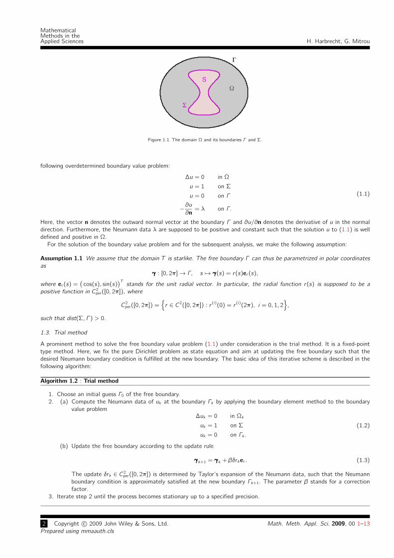
Let T ⊂ R2 denote a bounded domain with free boundary ∂T = Γ . Inside the domain T , we assume the existence of a simply

connected subdomain S ⊂ T with fixed boundary ∂S = Σ. The resulting annular domain T \ S is denoted by Ω and displayed in

Figure 1.1. Bernoulli’s free boundary problem consists now in seeking the domain Ω and the function u which both satisfy the

aMathematisches Institut, Universitat Basel, Rheinsprung 21, 4051 Basel, Switzerland.∗Correspondence to: E-mail: [email protected]

Math. Meth. Appl. Sci. 2009, 00 1–13 Copyright c© 2009 John Wiley & Sons, Ltd.

Prepared using mmaauth.cls [Version: 2009/09/02 v2.00]

MathematicalMethods in theApplied Sciences H. Harbrecht, G. Mitrou

K

1

Y

S

Figure 1.1. The domain Ω and its boundaries Γ and Σ.

following overdetermined boundary value problem:

∆u = 0 in Ω

u = 1 on Σ

u = 0 on Γ

−∂u∂n

= λ on Γ.

(1.1)

Here, the vector n denotes the outward normal vector at the boundary Γ and ∂u/∂n denotes the derivative of u in the normal

direction. Furthermore, the Neumann data λ are supposed to be positive and constant such that the solution u to (1.1) is well

defined and positive in Ω.

For the solution of the boundary value problem and for the subsequent analysis, we make the following assumption:

Assumption 1.1 We assume that the domain T is starlike. The free boundary Γ can thus be parametrized in polar coordinates

as

γγγ : [0, 2π]→ Γ, s 7→ γγγ(s) = r(s)er (s),

where er (s) =(

cos(s), sin(s))T

stands for the unit radial vector. In particular, the radial function r(s) is supposed to be a

positive function in C2per([0, 2π]), where

C2per([0, 2π]) =

r ∈ C2([0, 2π]) : r (i)(0) = r (i)(2π), i = 0, 1, 2

,

such that dist(Σ, Γ ) > 0.

1.3. Trial method

A prominent method to solve the free boundary value problem (1.1) under consideration is the trial method. It is a fixed-point

type method. Here, we fix the pure Dirichlet problem as state equation and aim at updating the free boundary such that the

desired Neumann boundary condition is fulfilled at the new boundary. The basic idea of this iterative scheme is described in the

following algorithm:

Algorithm 1.2 : Trial method

1. Choose an initial guess Γ0 of the free boundary.

2. (a) Compute the Neumann data of uk at the boundary Γk by applying the boundary element method to the boundary

value problem∆uk = 0 in Ωk

uk = 1 on Σ

uk = 0 on Γk .

(1.2)

(b) Update the free boundary according to the update rule

γγγk+1 = γγγk + βδrker . (1.3)

The update δrk ∈ C2per([0, 2π]) is determined by Taylor’s expansion of the Neumann data, such that the Neumann

boundary condition is approximately satisfied at the new boundary Γk+1. The parameter β stands for a correction

factor.

3. Iterate step 2 until the process becomes stationary up to a specified precision.

2 Copyright c© 2009 John Wiley & Sons, Ltd. Math. Meth. Appl. Sci. 2009, 00 1–13

Prepared using mmaauth.cls

H. Harbrecht, G. Mitrou

MathematicalMethods in theApplied Sciences

The use of a first order Taylor expansion when the free boundary is updated according to the Dirichlet boundary condition at

the boundary Γk has been proposed for example in [9, 24].

1.4. Organization of the article

The remainder of this article is organized as follows. In Section 2, after a brief review of results from shape sensitivity analysis,

we compute the Neumann data’s first order Taylor expansion around the actual free boundary. This yields a first update rule for

the free boundary. In Section 3, the numerical realization of the free boundary problem is introduced. First, the free boundary

is discretized in Subsection 3.1. Then, in Subsection 3.2, we present the boundary element method to determine the Neumann

data of the function u. Some numerical tests for the update rule (1.3) are performed in Subsection 3.3. They show numerical

difficulties, especially if the free boundary is not convex. Section 4 is thus dedicated to the convergence analysis of the trial

method, due to which we propose to modify the update rule such that the convergence is improved. The feasibility of the

resulting trial method is shown by numerical results in Subsection 4.4. Finally, in Section 5, the article’s conclusion is drawn.

2. Derivation of the update rule

2.1. Background in shape sensitivity analysis

We shall give a brief background in shape sensitivity analysis, necessary for our further computations. For all the details, especially

the proof of Lemma 2.4, we address the reader to [7, 15, 16, 19].

Let V : Ω→ R2 be a sufficiently smooth perturbation field which does not change the interior boundary Σ, i.e., V|Σ = 0.

Then, given a small parameter ε > 0, the perturbed domain Ωε = Ωε[V] is defined via

Ωε :=

(I + εV)(x) : x ∈ Ω. (2.1)

Consequently, the associated perturbation of the outer boundary Γ is

Γε := (I + εV

)(x) : x ∈ Γ.

On the domains Ω and Ωε with interior boundary Σ and outer boundaries Γ and Γε, respectively, the functions u and uε are

defined as the solution to the boundary value problems

∆u = 0 in Ω, ∆uε = 0 in Ωε,

u = 1 on Σ, uε = 1 on Σ, (2.2)

u = 0 on Γ, uε = 0 on Γε.

The relation between u and uε for small values of ε is subject of the shape sensitivity analysis. As an important concept, the

material derivative u is introduced. It is computed by pulling back uε to the unperturbed domain Ω, i.e., by differentiating

uε(x) :=(uε (I + εV)

)(x) = uε(xε).

Definition 2.1 The material derivative of u in the direction V is defined as the limit

u[V](x) :=duε[V](x)

dε

∣∣∣ε=0

= limε→0

uε[V](x)− u(x)

ε, x ∈ Ω.

In contrast, the direct differentiation of uε(x) leads to the local shape derivative.

Definition 2.2 The local shape derivative of u in the direction V is given by

δu[V](x) :=duε[V](x)

dε

∣∣∣ε=0

= limε→0

uε[V](x)− u(x)

ε, x ∈ Ω.

The relation between the material and the local shape derivative is expressed in the following remark.

Remark 2.3 The chain rule combines the material and the local shape derivative by the relation

u[V] = δu[V] + 〈∇u,V〉. (2.3)

The local shape derivative of u from the boundary value problem (2.2) reads as follows.

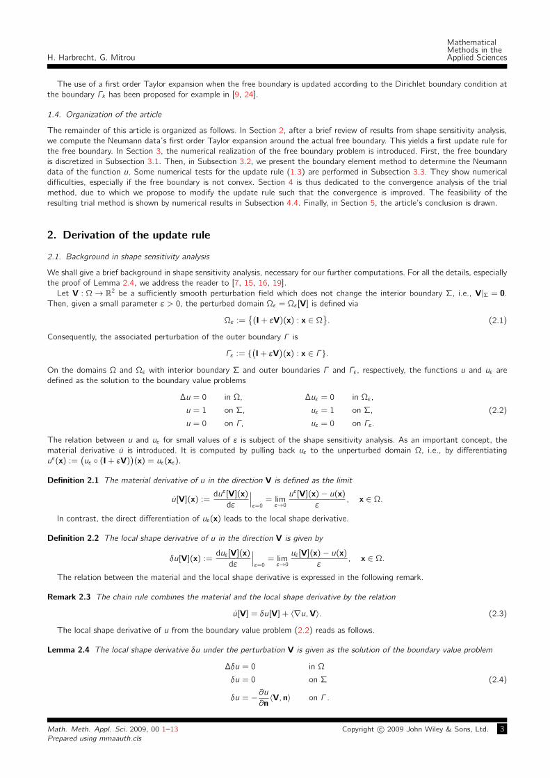
Lemma 2.4 The local shape derivative δu under the perturbation V is given as the solution of the boundary value problem

∆δu = 0 in Ω

δu = 0 on Σ (2.4)

δu = −∂u∂n〈V, n〉 on Γ .

Math. Meth. Appl. Sci. 2009, 00 1–13 Copyright c© 2009 John Wiley & Sons, Ltd. 3Prepared using mmaauth.cls


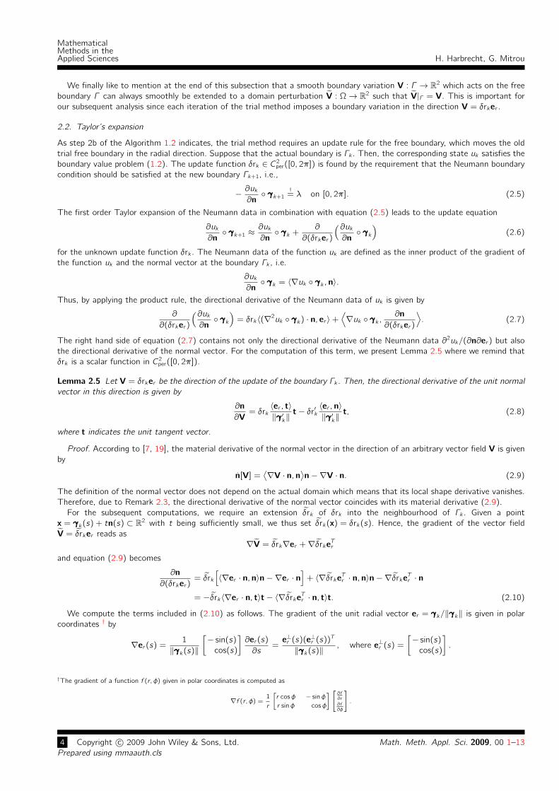
We finally like to mention at the end of this subsection that a smooth boundary variation V : Γ → R2 which acts on the free

boundary Γ can always smoothly be extended to a domain perturbation V : Ω→ R2 such that V|Γ = V. This is important for

our subsequent analysis since each iteration of the trial method imposes a boundary variation in the direction V = δrker .

2.2. Taylor’s expansion

As step 2b of the Algorithm 1.2 indicates, the trial method requires an update rule for the free boundary, which moves the old

trial free boundary in the radial direction. Suppose that the actual boundary is Γk . Then, the corresponding state uk satisfies the

boundary value problem (1.2). The update function δrk ∈ C2per([0, 2π]) is found by the requirement that the Neumann boundary

condition should be satisfied at the new boundary Γk+1, i.e.,

− ∂uk∂n γγγk+1

!= λ on [0, 2π]. (2.5)

The first order Taylor expansion of the Neumann data in combination with equation (2.5) leads to the update equation

∂uk∂n γγγk+1 ≈

∂uk∂n γγγk +

∂

∂(δrker )

(∂uk∂n γγγk

)(2.6)

for the unknown update function δrk . The Neumann data of the function uk are defined as the inner product of the gradient of

the function uk and the normal vector at the boundary Γk , i.e.

∂uk∂n γγγk = 〈∇uk γγγk , n〉.

Thus, by applying the product rule, the directional derivative of the Neumann data of uk is given by

∂

∂(δrker )

(∂uk∂n γγγk

)= δrk〈(∇2uk γγγk) · n, er 〉+

⟨∇uk γγγk ,

∂n

∂(δrker )

⟩. (2.7)

The right hand side of equation (2.7) contains not only the directional derivative of the Neumann data ∂2uk/(∂n∂er ) but also

the directional derivative of the normal vector. For the computation of this term, we present Lemma 2.5 where we remind that

δrk is a scalar function in C2per([0, 2π]).

Lemma 2.5 Let V = δrker be the direction of the update of the boundary Γk . Then, the directional derivative of the unit normal

vector in this direction is given by

∂n

∂V= δrk

〈er , t〉‖γγγ ′k‖

t− δr′k〈er , n〉‖γγγ ′k‖

t, (2.8)

where t indicates the unit tangent vector.

Proof. According to [7, 19], the material derivative of the normal vector in the direction of an arbitrary vector field V is given

by

n[V] =⟨∇V · n, n

⟩n−∇V · n. (2.9)

The definition of the normal vector does not depend on the actual domain which means that its local shape derivative vanishes.

Therefore, due to Remark 2.3, the directional derivative of the normal vector coincides with its material derivative (2.9).

For the subsequent computations, we require an extension δrk of δrk into the neighbourhood of Γk . Given a point

x = γγγk(s) + tn(s) ⊂ R2 with t being sufficiently small, we thus set δrk(x) = δrk(s). Hence, the gradient of the vector field

V = δrker reads as

∇V = δrk∇er +∇δrkeTr

and equation (2.9) becomes

∂n

∂(δrker )= δrk

[〈∇er · n, n〉n−∇er · n

]+ 〈∇δrkeTr · n, n〉n−∇δrkeTr · n

= −δrk〈∇er · n, t〉t− 〈∇δrkeTr · n, t〉t. (2.10)

We compute the terms included in (2.10) as follows. The gradient of the unit radial vector er = γγγk/‖γγγk‖ is given in polar

coordinates † by

∇er (s) =1

‖γγγk(s)‖

[− sin(s)

cos(s)

]∂er (s)

∂s=

e⊥r (s)(e⊥r (s))T

‖γγγk(s)‖ , where e⊥r (s) =

[− sin(s)

cos(s)

].

†The gradient of a function f (r, φ) given in polar coordinates is computed as

∇f (r, φ) =1

r

[r cosφ − sinφ

r sinφ cosφ

][ ∂f∂r

∂f∂φ

].





By use of this relation, the first term of the right hand side of (2.10) is calculated as

〈∇er · n, t〉t =⟨e⊥r (e⊥r )T

‖γγγk‖· n, t

⟩t =

tT e⊥r (e⊥r )Tn

‖γγγk‖t =〈e⊥r , t〉〈e⊥r , n〉‖γγγk‖

t. (2.11)

Exploiting the identities

〈e⊥r , t〉 = −〈er , n〉, 〈e⊥r , n〉 = 〈er , t〉 and〈er , n〉‖γγγk‖

=1

‖γγγ ′k‖,

(2.11) can be further simplified in accordance with

〈∇er · n, t〉t = −〈er , n〉〈er , t〉‖γγγk‖t = −〈er , t〉‖γγγ ′k‖

t. (2.12)

Employing again polar coordinates, the gradient of δrk is seen to be

∇δrk(γγγk(s) + tn(s)

)=

1

‖γγγk(s)‖

[− sin(s)

cos(s)

]δrk(s)′ = − e⊥r (s)

‖γγγk(s)‖δrk(s)′.

Consequently, the second term of the right hand side of (2.10) transforms to

〈∇δrkeTr · n, t〉t = − 1

‖γγγk‖δr′k〈e⊥r , t〉〈er , n〉t = δr′k

〈er , n〉‖γγγ ′k‖

t. (2.13)

The validity of (2.8) follows finally from plugging (2.12) and (2.13) into (2.10).

We proceed with the computation of the derivative of the Neumann data of uk in the direction V.

Lemma 2.6 The derivative of the Neumann data of the function uk , which satisfies the boundary value problem (1.2), in the

direction V = δrker is given by

∂

∂(δrker )

(∂uk∂n γγγk

)=

((∂2uk∂n2

γγγk)〈er , n〉+

( ∂2uk∂n∂t

γγγk)〈er , t〉

)δrk . (2.14)

Proof. We return to equation (2.7) and notice that the first term of the right-hand side of equation (2.7) is found by decomposing

the second order directional derivative of uk into its normal and tangential components as follows:

〈(∇2uk γγγk) · n, er 〉 = 〈(∇2uk γγγk) · n, n〉〈er , n〉+ 〈(∇2uk γγγk) · n, t〉〈er , t〉

=(∂2uk∂n2


( ∂2uk∂n∂t

γγγk)〈er , t〉. (2.15)

By inserting (2.8) and (2.15) into (2.7), we arrive at the directional derivative of the Neumann data at the boundary Γk :

∂

∂(δrker )

(∂uk∂n γγγk

)=

[(∂2uk∂n2


( ∂2uk∂n∂t

γγγk)〈er , t〉+

(∂uk∂t γγγk

) 〈er , t〉‖γγγ ′k‖

]δrk −

(∂uk∂t γγγk

) 〈er , n〉‖γγγ ′k‖

δr′k . (2.16)

Finally, due to the Dirichlet boundary condition uk = 0 at Γk , the tangential derivative of uk vanishes and (2.14) follows.

The directional derivative of the Neumann data of the function uk , as it is given in (2.16), coincides with the derivative which

has been proven in [18, Theorem 3.11] in the context of inverse scattering problems. However, by using results from shape

sensitivity analysis, we were able to obtain this relation by a much simpler proof.

2.3. Update equation

With the help of (2.14), we are able to formulate the update equation for the unknown function δrk in Lemma 2.7.

Lemma 2.7 The update equation, which is obtained by combining (2.5) and (2.6), reads as

λ =

[κ(∂uk∂n γγγk

)〈er , n〉 −

∂

∂t

(∂uk∂n γγγk

)〈er , t〉

]δrk −

∂uk∂n γγγk , (2.17)

where κ denotes the curvature κ = −〈γγγ ′′k , n〉/‖γγγ′k‖

2.



Proof. The combination of the Taylor expansion (2.6) with the requirement (2.5) at the next boundary Γk+1 induces the update

equation

−λ =∂uk∂n γγγk +

∂

∂(δrker )

(∂uk∂n γγγk

).

Due to (2.14), this equation can be transformed to

− λ =∂uk∂n γγγk +

[(∂2uk∂n2


( ∂2uk∂n∂t

γγγk)〈er , t〉

]δrk . (2.18)

We compute the second order directional derivative ∂2uk/(∂n∂t) by differentiating ∂uk/∂n with respect to s. Namely, we

have

∂

∂s

(∂uk∂n γγγk

)= ‖γγγ ′k‖

∂2uk∂n∂t

γγγk +⟨∇uk γγγk ,

∂n

∂s

⟩. (2.19)

In view of ∂n/∂s = κ‖γγγ ′k‖t and the homogeneous Dirichlet boundary condition at Γk , equation (2.19) implies that

∂2uk∂n∂t

=∂

∂t

(∂uk∂n

)− κ∂uk

∂t=∂

∂t

(∂uk∂n

). (2.20)

According to our smoothness assumptions, the terms ∂2uk/∂n2 and ∂2uk/∂t2 are coupled via the Laplace equation, i.e.,

∆uk =∂2uk∂n2

+∂2uk∂t2

= 0.

Hence, the second order directional derivative ∂2uk/∂n2 can be found from the second order derivative of uk with respect to s:

∂2(uk γγγk)

∂s2= 〈(∇2uk γγγk) · γγγ ′k , γγγ

′k〉+ 〈∇uk γγγk , γγγ

′′k〉

= ‖γγγ ′k‖2(∂2uk∂t2

γγγk)

+ 〈γγγ ′′k , t〉(∂uk∂t γγγk

)+ 〈γγγ ′′k , n〉

(∂uk∂n γγγk

).

This means that

∂2uk∂n2

γγγk = − 1

‖γγγ ′k‖2

∂2(uk γγγk)

∂s2+〈γγγ ′′k , t〉‖γγγ ′k‖2

(∂uk∂t γγγk

)− κ

(∂uk∂n γγγk

).

Due to the homogeneous Dirichlet boundary condition at Γk , the tangential derivative of uk and the second oder derivative of

uk with respect to s disappear. This yields

∂2uk∂n2

= −κ∂uk∂n

. (2.21)

The desired equation (2.17) is now an immediate consequence after inserting the equations (2.20) and (2.21) into (2.18).

3. Discretization

3.1. Approximation of the free boundary

For the numerical computations, we discretize the radial function r nk , associated with the boundary Γk , by a finite Fourier series

according to

r nk (s) = a0 +

n−1∑i=1

ai cos(is) + bi sin(is)

+ an cos(ns). (3.1)

This obviously ensures that r nk is always an element of C2per([0, 2π]). To determine the update function δr nk , represented likewise

by a finite Fourier series, we insert the m ≥ 2n equidistantly distributed points si = 2πi/m into the update equation

F (δrk) :=

[κ(∂uk∂n γγγk

)〈er , n〉 −

∂

∂t

(∂uk∂n γγγk

)〈er , t〉

]δrk −

∂uk∂n γγγk

!= λ. (3.2)

To solve this equation, we reformulate it as a discrete least-squares problem which can simply be solved via the normal equations.





Y

K0

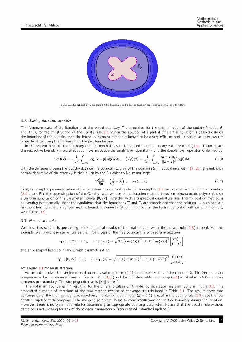
Figure 3.1. Solutions of Bernoulli’s free boundary problem in case of an x-shaped interior boundary.

3.2. Solving the state equation

The Neumann data of the function u at the actual boundary Γ are required for the determination of the update function δr

and, thus, for the construction of the update rule 1.3. When the solution of a partial differential equation is desired only on

the boundary of the domain, then the boundary element method is known to be a very efficient tool. In particular, it enjoys the

property of reducing the dimension of the problem by one.

In the present context, the boundary element method has to be applied to the boundary value problem (1.2). To formulate

the respective boundary integral equation, we introduce the single layer operator V and the double layer operator K defined by(Vρ)

(x) = − 1

2π

∫Σ∪Γk

log ‖x− y‖ρ(y) dσy,(Kρ)

(x) =1

2π

∫Σ∪Γk

〈x− y, ny〉‖x− y‖2

ρ(y) dσy (3.3)

with the densities ρ being the Cauchy data on the boundary Σ ∪ Γk of the domain Ωk . In accordance with [17, 21], the unknown

normal derivative of the state uk is then given by the Dirichlet-to-Neumann map:

V ∂uk∂n

=(1

2+K

)uk on Σ ∪ Γk . (3.4)

First, by using the parametrization of the boundaries as it was described in Assumption 1.1, we parametrize the integral equation

(3.4), too. For the approximation of the Cauchy data, we use the collocation method based on trigonometric polynomials on

a uniform subdivision of the parameter interval [0, 2π]. Together with a trapezoidal quadrature rule, this collocation method is

converging exponentially under the conditions that the boundaries Σ and Γk are smooth and that the solution uk is an analytic

function. For more details concerning this boundary element method, in particular, the technique to deal with singular integrals,

we refer to [13].

3.3. Numerical results

We close this section by presenting some numerical results of the trial method when the update rule (1.3) is used. For this

example, we have chosen an ellipse as the initial guess of the free boundary Γ0 with parametrization

γγγ0 : [0, 2π]→ Γ0, s 7→ γγγ0(s) =

√0.1(

cos(2s))2

+ 0.12(

sin(2s))2

[cos(s)

sin(s)

]and an x-shaped fixed boundary Σ with parametrization

γγγΣ : [0, 2π]→ Σ, s 7→ γγγΣ(s) =

√0.01

(cos(2s)

)2+ 0.05

(sin(2s)

)2

[cos(s)

sin(s)

],

see Figure 3.1 for an illustration.

We intend to solve the overdetermined boundary value problem (1.1) for different values of the constant λ. The free boundary

is represented by 16 degrees of freedom (i.e. n = 8 in (3.1)) and the Dirichlet-to-Neumann map (3.4) is solved with 600 boundary

elements per boundary. The stopping criterion is ‖δr‖ < 10−8.

The optimum boundaries Γ ? resulting for the different values of λ under consideration are also found in Figure 3.1. The

associated numbers of iterations of the trial method needed to converge are tabulated in Table 3.1. The results show that

convergence of the trial method is achieved only if a damping parameter (β = 0.1) is used in the update rule (1.3), see the row

entitled “update with damping”. The damping parameter helps to avoid oscillations of the free boundary during the iteration.

However, there is no systematic rule for determining an appropriate damping parameter. Notice that the update rule without

damping is not working for any of the chosen parameters λ (row entitled “standard update”).



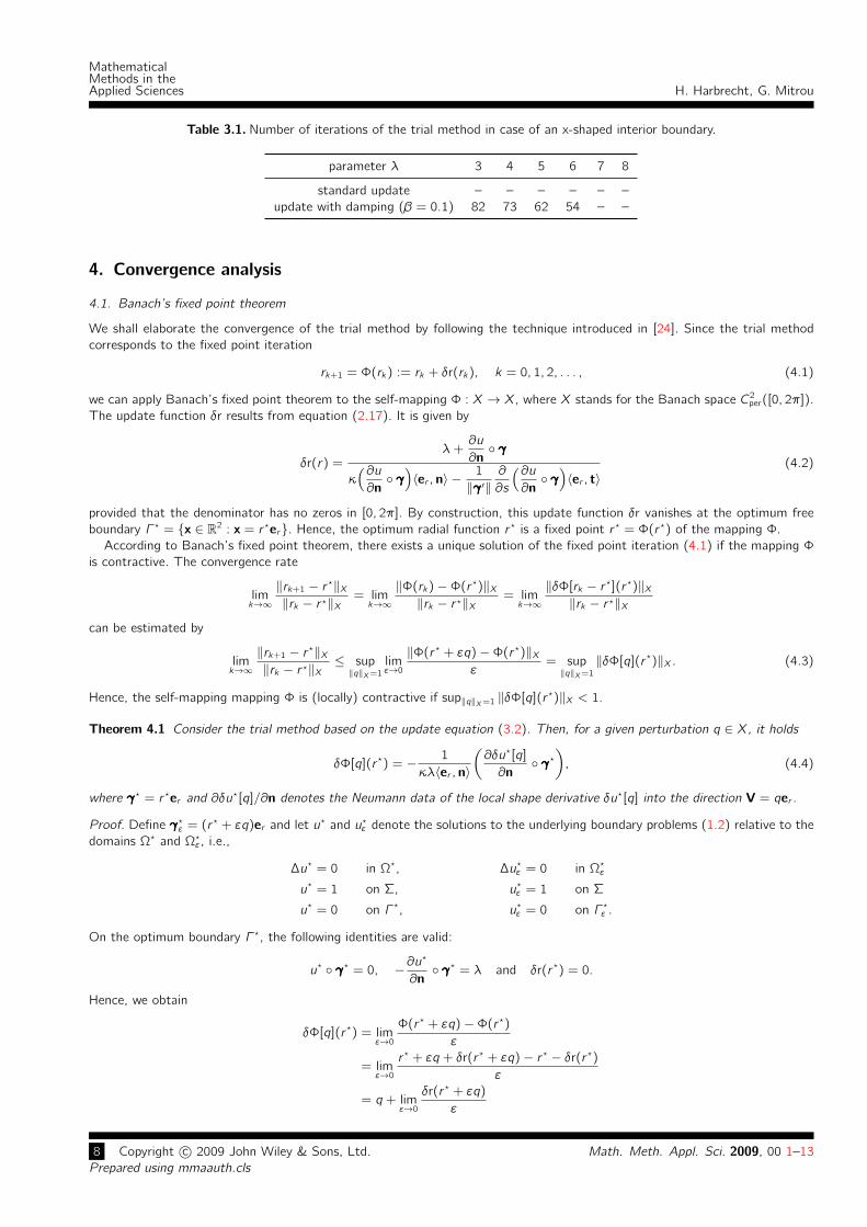
Table 3.1. Number of iterations of the trial method in case of an x-shaped interior boundary.

parameter λ 3 4 5 6 7 8

standard update – – – – – –

update with damping (β = 0.1) 82 73 62 54 – –

4. Convergence analysis

4.1. Banach’s fixed point theorem

We shall elaborate the convergence of the trial method by following the technique introduced in [24]. Since the trial method

corresponds to the fixed point iteration

rk+1 = Φ(rk) := rk + δr(rk), k = 0, 1, 2, . . . , (4.1)

we can apply Banach’s fixed point theorem to the self-mapping Φ : X → X, where X stands for the Banach space C2per([0, 2π]).

The update function δr results from equation (2.17). It is given by

δr(r) =λ+

∂u

∂n γγγ

κ(∂u∂n γγγ)〈er , n〉 −

1

‖γγγ ′‖∂

∂s

(∂u∂n γγγ)〈er , t〉

(4.2)

provided that the denominator has no zeros in [0, 2π]. By construction, this update function δr vanishes at the optimum free

boundary Γ ? = x ∈ R2 : x = r ?er. Hence, the optimum radial function r ? is a fixed point r ? = Φ(r ?) of the mapping Φ.

According to Banach’s fixed point theorem, there exists a unique solution of the fixed point iteration (4.1) if the mapping Φ

is contractive. The convergence rate

limk→∞

‖rk+1 − r ?‖X‖rk − r ?‖X

= limk→∞

‖Φ(rk)−Φ(r ?)‖X‖rk − r ?‖X

= limk→∞

‖δΦ[rk − r ?](r ?)‖X‖rk − r ?‖X

can be estimated by

limk→∞

‖rk+1 − r ?‖X‖rk − r ?‖X

≤ sup‖q‖X=1

limε→0

‖Φ(r ? + εq)−Φ(r ?)‖Xε

= sup‖q‖X=1

‖δΦ[q](r ?)‖X . (4.3)

Hence, the self-mapping mapping Φ is (locally) contractive if sup‖q‖X=1 ‖δΦ[q](r ?)‖X < 1.

Theorem 4.1 Consider the trial method based on the update equation (3.2). Then, for a given perturbation q ∈ X, it holds

δΦ[q](r ?) = − 1

κλ〈er , n〉

(∂δu?[q]

∂n γγγ?

), (4.4)

where γγγ? = r ?er and ∂δu?[q]/∂n denotes the Neumann data of the local shape derivative δu?[q] into the direction V = qer .

Proof. Define γγγ?ε = (r ? + εq)er and let u? and u?ε denote the solutions to the underlying boundary problems (1.2) relative to the

domains Ω? and Ω?ε, i.e.,

∆u? = 0 in Ω?, ∆u?ε = 0 in Ω?ε

u? = 1 on Σ, u?ε = 1 on Σ

u? = 0 on Γ ?, u?ε = 0 on Γ ?ε .

On the optimum boundary Γ ?, the following identities are valid:

u? γγγ? = 0, −∂u?

∂n γγγ? = λ and δr(r ?) = 0.

Hence, we obtain

δΦ[q](r ?) = limε→0

Φ(r ? + εq)−Φ(r ?)

ε

= limε→0

r ? + εq + δr(r ? + εq)− r ? − δr(r ?)

ε

= q + limε→0

δr(r ? + εq)

ε





with

δr(r ? + εq) =λ+

∂u?ε∂nε γγγ?ε

κ(∂u?ε∂nε γγγ?ε

)〈er , nε〉 −

1

‖γγγ?ε ′‖∂

∂s

(∂u?ε∂nε γγγ?ε

)〈er , tε〉

. (4.5)

We split the enumerator of (4.5) as follows

∂u?ε∂nε γγγ?ε + λ =

∂u?ε∂nε γγγ?ε −

∂u?

∂n γγγ?

= 〈∇u?ε γγγ?ε, nε〉 − 〈∇u?ε γγγ?, nε〉+ 〈∇u?ε γγγ?, nε〉 − 〈∇u?ε γγγ?, n〉+ 〈∇u?ε γγγ?, n〉 − 〈∇u? γγγ?, n〉.

This yields1

ε

(∂u?ε∂nε γγγ?ε + λ

)ε→0−→ ∂

∂(qer )

(∂u?∂n γγγ?

)+⟨∇u? γγγ?, ∂n

∂(qer )

⟩+∂δu?[q]

∂n γγγ?. (4.6)

Herein, in view of equation (2.14), the derivative of the Neumann data of u? in the direction V = qer is given by

∂

∂(qer )

(∂u?∂n γγγ?

)=

[(∂2u?

∂n2 γγγ?

)〈er , n〉+

( ∂2u?

∂n∂t γγγ?

)〈er , t〉

]q.

The Neumann data of the local shape derivative δu?[q] at the boundary Γ ? are also contained in (4.6). The local shape derivative

satisfies the boundary value problem (2.4). Moreover, the derivative of the normal vector in the direction V = qer fulfills

∂n

∂(qer )= q〈er , t〉‖γγγ?′‖ t− q′ 〈er , n〉‖γγγ?′‖ t (4.7)

(details about (4.7) are reported in Lemma 2.5). Since the derivative (4.7) of the normal vector is pointing only to the tangential

direction, the third term on the right hand side of (4.6) vanishes due to u?’s homogeneous Dirichlet data at Γ ? and we arrive at

limε→0

1

ε

(∂u?ε∂nε γγγ?ε + λ

)=∂δu?[q]

∂n γγγ? +

[(∂2u?

∂n2 γγγ?

)〈er , n〉+

( ∂2u?

∂n∂t γγγ?

)〈er , t〉

]q. (4.8)

Finally, we obtain (4.4) by inserting (4.8) into (4.5) and taking into account (2.21) and −∂u?/∂n γγγ? = λ.

On the one hand, the convergence of the trial method is ensured when the mapping Φ is contractive. This is the case if the

norm of (4.4) at Γ ? is smaller than 1, i.e., if

‖δΦ[q](r ?)‖X =

∥∥∥∥ 1

κλ〈er , n〉

(∂δu?[q]

∂n γγγ?

)∥∥∥∥X

< 1.

On the other hand, since for nontrivial boundary perturbations the prescribed Dirichlet data at Γ ? in the boundary value problem

(2.4) are non-zero, we conclude δu?[q] 6= 0. Therefore, in case of convergence, we can only expect a linear convergence order

of the trial method.

A much more important consequence of Theorem 4.1 is that the sign of the denominator in (4.4) can change, i.e., the

denominator might have zeros and the trial method might thus not converge. Since λ is a positive constant and 〈er , n〉 is always

positive for starlike domains, this happens if the curvature κ changes its sign. Hence, the trial method is expected to converge

only when the optimum boundary Γ ? is convex since the curvature is then positive in a neighbourhood. This observation provides

a satisfactory explanation for the results in Section 3.3, where we found that the trial method is converging for those values of

λ where the optimum boundary is convex.

4.2. Modified update rule

Our suggestion to overcome this difficulty is to modify the update rule. Namely, instead of (4.2), we propose to use

∆r(r) := κ(r)δr(r) =λ+

∂u

∂n γγγ(∂u

∂n γγγ)〈er , n〉 −

〈er , t〉κ‖γγγ ′‖

∂

∂s

(∂u∂n γγγ) . (4.9)

The self-mapping Φ is thus modified in accordance with

Φm : X → X, r 7→ Φm(r) = r + ∆r(r). (4.10)



As in Subsection 4.1, we compute the derivative of Φm at the point r ? in the direction qer

δΦm[q](r ?) = limε→0

Φm(r ? + εq)−Φm(r ?)

ε= q + lim

ε→0

∆r(r ? + εq)

ε

and find, likewise to Theorem 4.1, that

δΦm[q](r ?) = q − 1

λ〈er , n〉

(∂δu?[q]

∂n γγγ? + κλq〈er , n〉

)= (1− κ)q − 1

λ〈er , n〉

(∂δu?[q]

∂n γγγ?

)(4.11)

For the modified self-mapping Φm, we obtain thus a denominator which is always positive in a neighbourhood of the optimum

boundary Γ ?, as λ > 0 and 〈er , n〉 > 0 holds in case of starlike domains. Therefore, with the modified update function (4.9), we

can expect convergence not only in case of convex optimum boundaries but also in general.

4.3. Speeding up the convergence

A further modification of the self-mapping Φ is obtained by the ansatz

Φi : X → X, r 7→ Φi(r) = r + β(r)∆r(r) (4.12)

with ∆r(r) from (4.9). The function β(r) : [0, 2π]→ R should improve the trial method in two regards. Firstly, it should avoid

the necessity to conduct endless tests of the trial method until an appropriate damping parameter is found. Secondly, the function

β(r) should be chosen such that the speed of convergence is increased.

Since ∆r(r ?) = 0 by construction, the derivative of Φi at the point r ? in the direction qer is given by

δΦi [q](r ?) = q + β(r ?) limε→0

∆r(r ? + εq)

ε.

In view of (4.10) and (4.11), this derivative reads as

δΦi [q](r ?) = q − β(r ?)

[1

λ〈er , n〉

(∂δu?[q]

∂n γγγ?

)+ κq

]. (4.13)

The above goals are achieved if we define the function β(r) such that the derivative from (4.13) vanishes for the direction

q := limk→∞(rk − r ?)/‖rk − r ?‖X provided that this limit exists. Since, however, r ? is not known beforehand, q would not be

accessible even in the case of existence. Nevertheless, the choice qk = rk − rk−1 with q0 = 1 is a good approximation. Hence,

we should define the function β by

β(rk) =

[1

λ〈er , n〉

(∂δuk [qk ]

∂n γγγk

)+ κqk

]−1

qk . (4.14)

Herein, the local shape derivative ∂δuk [qk ]/∂n can be computed in complete analogy to the Neumann data of uk by using the

Dirichlet-to-Neumann map, as it was described in Section 3. Hence, one additional solve of the Dirichlet-to-Neumann map is

necessary per iteration step.

Remark 4.2 The function β(rk) from (4.14) is chosen such that δΦi [qk ](r ?)→ 0 as k →∞. However, there are other reasonable

definitions with this property. A possible simplification which we use in our particular implementation would be to insert the

Neumann data of the solution to the boundary value problem

∆δu = 0 in Ωk

δu = 0 on Σ

δu = λqk〈er, n〉 on Γk

instead of the Neumann data of the local shape derivative δuk [qk ] into (4.14). As a further alternative, one may also use

β(rk) =

∂δuk [qk ]

∂n γγγk(∂u

∂n γγγk

)〈er , n〉 −

〈er , t〉κ‖γγγ ′k‖

∂

∂s

(∂u∂n γγγk

) + κqk

−1

qk .

Numerical tests do not clearly show the superiority of one of these choices.





0

Figure 4.1. Solutions of Bernoulli’s free boundary problem in case of a random interior boundary.

Table 4.1. Number of boundary updates of the trial method in case of a random interior boundary.

parameter λ 8 10 12 14 16

modified update with damping (β = 0.01) 179 146 130 122 125

improved modified update 114 94 92 101 92

4.4. Numerical results

In our first example, we choose the initial guess Γ0 of the trial method boundary to be an ellipse parametrized by

γγγ0 : [0, 2π]→ Γ0, s 7→ γγγ0(s) =

√0.1(

cos(2s))2

+ 0.11(

sin(2s))2

[cos(s)

sin(s)

].

The fixed interior boundary Σ is a randomly generated boundary as seen in Figure 4.1. The solutions of the free boundary problem

for different values of λ are also found in this figure. For the numerical computations, we have used 50 degrees of freedom for

the representation of the free boundary and 600 boundary elements per boundary. The stopping criterion has been ‖∆r‖ < 10−8.

In Table 4.1, the number of iterations, which are needed by the trial method to converge, are tabulated. There are no results

for the standard update rule (1.3) as in this case the optimum boundary is non-convex for all values of λ under consideration,

and thus the associated trial method did not converge. In contrast, the trial method based on the modified update rule with

update function (4.9) is converging (row entitled “modified update with damping”). Nevertheless, also in this case, a damping

parameter (β = 0.01) is essential for the convergence. By computing the function β(r) from (4.14), we avoid not only the costly

determination of the damping parameter β, but we also achieve a slight speed-up of the convergence of the trial method (row

entitled “improved modified update”).

The second example refers to a domain Ω which consists of four interior boundaries Σ = Σ1 ∪Σ2 ∪Σ3 ∪Σ4 and one outer free

boundaries Γ . We solve the associated Bernoulli free boundary problem, whose solutions for different values λ of the Neumann

data are depicted in Figure 4.2. For the numerical simulation have been used: 400 boundary elements per boundary, i.e., 2000

in all, and 30 degrees of freedom for the representation of the free boundary. The initial guess Γ0 is a properly scaled circle and

the stopping criterion is again ‖∆r‖ < 10−8.

Table 4.2. Number of boundary updates of the trial method in case of several interior boundaries.

parameter λ 2 4 6 8 10 12

update with damping (β = 0.05) 125 – – – – –

modified update with damping (β = 0.05) 117 65 49 45 46 51

improved modified update 118 79 68 48 51 –

As it is shown in Table 4.2, we achieve convergence for the trial method and for all the chosen values of the parameter λ when

the modified update rule (4.9) with damping parameter β = 0.05 is applied. For the same damping parameter, the standard



1

2

4

3

0

Figure 4.2. Solutions of Bernoulli’s free boundary problem in case of several interior boundaries.

update rule (4.2) converges only for λ = 2, as the optimum boundary is convex for this value. The improved modified update

rule shows in this case a behaviour which is similar to that of the modified update rule (4.9) with damping parameter.

5. Conclusion

In contrast to the trial method which updates according to the Dirichlet data, very few results can be found in the literature

about the trial method which updates according to the Neumann data. Here, we elucidated the theoretical background of the

latter method and analyzed its convergence. Furthermore, to the best of our knowledge, we are the first who implemented this

trial method and presented numerically results in case of more general boundaries and not only axially symmetric ones. For these

reasons, we strongly believe that valuable results on this trial method have been achieved in this article, with the most important

one being the stabilization of the update equation so that the trial method converges also in case of a nonconvex optimum free

boundary.

Acknowledgement

The authors acknowledge the support of this research by the DFG priority program SPP 1253 Optimization with PDEs and by

the SNF through the project No. 200021 137668.

References

1. A. Acker, Convergence results for an analytical trial free-boundary method, IMA J. Numer. Anal., 8 (1988), pp. 357–364.

2. , On the geometric form of Bernoulli configurations, Math. Methods Appl. Sci., 10 (1988), pp. 1–14.

3. H. W. Alt and L. A. Caffarelli, Existence and regularity for a minimum problem with free boundary, J. Reine Angew. Math., 325 (1981),

pp. 105–144.

4. A. Beurling, On free-boundary problems for the Laplace equation, Sem. on analytic functions, Inst. Adv. Stud. Princeton, (1957),

pp. 248–263.

5. F. Bouchon, S. Clain, and R. Touzani, Numerical solution of the free boundary Bernoulli problem using a level set formulation, Comput.

Methods Appl. Mech. Engrg., 194 (2005), pp. 3934–3948.

6. C. W. Cryer, A survey of trial-boundary methods for the numerical solution of free boundary problems, MRC Techn. Summary Rep.,

1693, (1976).

7. M. C. Delfour and J.-P. Zolesio, Shapes and geometries: Metrics, analysis, differential calculus, and optimization, vol. 22 of Advances

in Design and Control, Society for Industrial and Applied Mathematics (SIAM), Philadelphia, PA, 2nd ed., 2011.

8. K. Eppler and H. Harbrecht, Tracking Neumann data for stationary free boundary problems, SIAM J. Control Optim., 48 (2009/10),

pp. 2901–2916.

9. M. Flucher and M. Rumpf, Bernoulli’s free-boundary problem, qualitative theory and numerical approximation, J. Reine Angew. Math.,

486 (1997), pp. 165–204.

10. H. Harbrecht and G. Mitrou. Improved trial methods for a class of generalized Bernoulli problems. Preprint 2013-22, Mathematisches

Institut, Universitat Basel, Switzerland, 2013.





11. K. Ito, K. Kunisch and G. Peichl, Variational approach to shape derivatives for a class of Bernoulli problems, J. Math. Anal. Appl.,

314 (2006), pp. 126–149.

12. K. Karkkainen and T. Tiihonen, Free surfaces: shape sensitivity analysis and numerical methods, Internat. J. Numer. Methods Engrg.,

44 (1999), pp. 1079–1098.

13. R. Kress, Linear integral equations, vol. 82 of Applied Mathematical Sciences, Springer, New York, 2nd ed., 1999.

14. C. M. Kuster, P. A. Gremaud, and R. Touzani, Fast numerical methods for Bernoulli free boundary problems, SIAM J. Sci. Comput.,

29 (2007), pp. 622–634.

15. F. Murat and J. Simon, Etude de probleme d’optimal design, in Proceedings of the 7th IFIP Conference on Optimization Techniques:

Modeling and Optimization in the Service of Man, Part 2, Springer, Berlin-Heidelberg-New York, 1976, pp. 54–62.

16. O. Pironneau, Optimal shape design for elliptic systems, Springer series in computational physics, Springer, New York, 1984.

17. S. Sauter and C. Schwab, Boundary Element Methods, Springer, Berlin-Heidelberg, 2010.

18. P. Serranho, A hybrid method for inverse obstacle scattering problems, PhD thesis, Georg-August-Universitat Gottingen, 2007.

19. J. Sokolowski and J.-P. Zolesio, Introduction to shape optimization: Shape sensitivity analysis, vol. 16 of Springer Series in

Computational Mathematics, Springer, Berlin, 1992.

20. R. V. Southwell and G. Vaisey, Relaxation methods applied to engineering problems. XII. Fluid motions characterized by ‘free’ stream-

lines, Philos. Trans. Roy. Soc. London. Ser. A., 240 (1946), pp. 117–161.

21. O. Steinbach, Numerical Approximation Methods for Elliptic Boundary Value Problems. Finite and Boundary Elements, Springer,

New York, 2008.

22. D. E. Tepper, Free boundary problem, SIAM J. Math. Anal., 5 (1974), 841–846.

23. T. Tiihonen, Shape optimization and trial methods for free boundary problems, RAIRO Model. Math. Anal. Numer., 31 (1997),

pp. 805–825.

24. T. Tiihonen and J. Jarvinen, On fixed point (trial) methods for free boundary problems, in Free boundary problems in continuum

mechanics (Novosibirsk, 1991), vol. 106 of Internat. Ser. Numer. Math., Birkhauser, Basel, 1992, pp. 339–350.


_______________________________________________________________________

Preprints are available under http://math.unibas.ch/research/publications/

LATEST PREPRINTS

No. Author: Title

2013-01 H. Harbrecht, M. Peters

Comparison of Fast Boundary Element Methods on Parametric Surfaces

2013-02 V. Bosser, A. Surroca

Elliptic Logarithms, Diophantine Approximation and the Birch and

Swinnerton-Dyer Conjecture

2013-03 A. Surroca Ortiz

Unpublished Talk: On Some Conjectures on the Mordell-Weil and the Tate-

ShafarevichGgroups of an Abelian Variety

2013-04 V. Bosser, A. Surroca

Upper Bound for the Height of S-Integral Points on Elliptic Curves

2013-05 Jérémy Blanc, Jean-Philippe Furter, Pierre-Marie Poloni

Extension of Automorphisms of Rational Smooth Affine Curves

2013-06 Rupert L. Frank, Enno Lenzmann, Luis Silvestre

Uniqueness of Radial Solutions for the Fractional Laplacian

2013-07 Michael Griebel, Helmut Harbrecht

On the convergence of the combination technique

2013-08 Gianluca Crippa, Carlotta Donadello, Laura V. Spinolo

Initial-Boundary Value Problems for Continuity Equations with BV

Coefficients

2013-09 Gianluca Crippa, Carlotta Donadello, Laura V. Spinolo

A Note on the Initial-Boundary Value Problem for Continuity Equations

with Rough Coefficients

2013-10 Gianluca Crippa

Ordinary Differential Equations and Singular Integrals

2013-11 G. Crippa, M. C. Lopes Filho, E. Miot, H. J. Nussenzveig Lopes

Flows of Vector Fields with Point Singularities and the Vortex-Wave System

2013-12 L. Graff, J. Fender, H. Harbrecht, M. Zimmermann

Key Parameters in High-Dimensional Systems with Uncertainty

2013-13 Jérémy Blanc, Immanuel Stampfli

Automorphisms of the Plane Preserving a Curve

LATEST PREPRINTS

No. Author: Title

Preprints are available under http://www.math.unibas.ch/preprints

2013-14 Jérémy Blanc, Jung Kyu Canci

Moduli Spaces of Quadratic Rational Maps with a Marked Periodic Point of

Small Order

2013-15 Marcus J. Grote, Johannes Huber, Drosos Kourounis, Olaf Schenk

Inexact Interior-Point Method for Pde-Constrained Nonlinear Optimization

2013-16 Helmut Harbrecht, Florian Loos

Optimization of Current Carrying Multicables

2013-17 Daniel Alm, Helmut Harbrecht, Ulf Krämer

The H2-Wavelet Method

2013-18 Helmut Harbrecht, Michael Peters, Markus Siebenmorgen

Multilevel Accelerated Quadrature for PDEs with Log-Normal Distributed

Random Coefficient*

2013-19 Jérémy Blanc, Serge Cantat

Dynamical Degrees of Birational Transformations of Projective Surfaces

2013-20 Jérémy Blanc, Frédéric Mangolte

Cremona Groups of Real Surfaces

2013-21 Jérémy Blanc, Igor Dolgachev

Automorphisms of Cluster Algebras of Rank 2

2013-22 Helmut Harbrecht, Giannoula Mitrou

Improved Trial Methods for a Class of Generalized Bernoulli Problems

2013-23 Helmut Harbrecht, Johannes Tausch

On Shape Optimization with Parabolic State Equation

2013-24 Zoé Chatzidakis, Dragos Ghioca, David Masser, Guillaume Maurin

Unlikely, Likely and Impossible Intersections without Algebraic Groups

2013-25 Assyr Abdulle, Marcus J. Grote, Christian Stohrer

Finite Element Heterogeneous Multiscale Method for the Wave Equations :

Long Time Effects

2013-26 Luigi Ambrosio and Gianluca Crippa

Continuity Equations and ODE Flows with Non-Smooth Velocity

2013-27 Andriy Regeta

Lie Subalgebras of Vector Fields and the Jacobian Conjecture

2013-28 Helmut Harbrecht, Michael Peters, Markus Siebenmorgen

Tractability of the Quasi-Monte Carlo Quadrature with Halton Points for

Elliptic Pdes with Random Diffusion

LATEST PREPRINTS

No. Author: Title

Preprints are available under http://www.math.unibas.ch/preprints

2013-29 Helmut Harbrecht, Giannoula Mitrou

Stabilization of the Trial Method for the Bernoulli Problem in Case of

Prescribed Dirichlet Data

Documents

Stabilization of the Trial Method for the Bernoulli ... fileWith the help of shape sensitivity analysis and Banach’s xed-point theorem, we shed light on the convergence of the respective