Stabilizing compensators for linear time-varying differential systems

Stabilizing compensators for linear time-varyingdifferential systems

International Journal of Control 2015, DOI: 10.1080/00207179.2015.1091949

Ulrich OberstInstitut für Mathematik, Universität Innsbruck

Technikerstrasse 13, A-6020 Innsbruck, Austriaemail: [email protected]

September 5, 2015

Abstract

In this paper we describe a constructive test to decide whether a given lineartime-varying (LTV) differential system admits a stabilizing compensator for thecontrol tasks of tracking, disturbance rejection or model matching and constructand parametrize all of them if at least one exists. In analogy to the linear time-invariant (LTI) case the ring of stable rational functions, noncommutative in theLTV situation, and the Kucera-Youla parametrization play prominent parts in thetheory. We transfer Blumthaler’s thesis from the LTI to the LTV case and sharpen,complete and simplify the corresponding results in the book ’Linear Time-VaryingSystems’ by Bourlès and Marinescu.

AMS-classification: 93B52, 93D15, 93B25, 93C05, 93D20, 34H15Key-words: behavior, time-varying, stabilizing compensator, tracking, disturbance re-jection, model matching, exponential stability

1 Introduction(i) Results: In this paper we describe a constructive test to decide whether a given lin-ear time-varying (LTV) differential system admits a stabilizing compensator for thecontrol tasks of tracking, disturbance rejection or model matching and construct andparametrize all stabilizing compensators if at least one exists.(ii) Algebra and analysis: It turns out that the famous Kucera-Youla parametrizationand its application to the solution of various control tasks can be generalized fromstandard linear time-invariant (LTI) systems to LTV systems. The parametrization isan algebraic result and requires the proper choice of the used algebraic data, in par-ticular of the ring K of time-varying coefficient functions and of the associated ringA of differential operators with its associated module theory. On the other hand, thecomponents of the system trajectories are either smooth functions of the time-variablet or distributions whose stability refers to the behavior of these trajectories for t→∞and is defined by analytic conditions. In the LTI case all essential stability results canbe reduced to the purely algebraic fact that certain complex polynomials have only ze-ros with negative real part. In the LTV case the reduction of stability and stabilization

1

1 INTRODUCTION 2

problems to algebraic and algorithmic ones and the choice of the considered systems,algebraic and analytic data are more difficult than in the LTI case.(iii) Background: In this paper we describe systems as suitably defined behaviors anduse the weak exponential stability (w.e.s.), shortly just stability, of autonomous behav-iors. These notions were introduced and discussed in the recent paper [7] whose mainresults are recalled in the next lines and, with more details, in Section 2. The trajec-tories of a stable autonomous behavior converge to 0 for t → ∞ with decay factorsexp (−αtµ) where α, µ > 0. We use the differential field K of locally convergentPuiseux series and its associated skew-polynomial algebra A := K[∂] of differentialoperators with varying coefficients in K. This ring is noncommutative in contrast to thestandard commutative polynomial algebra C[∂] of differential operators with constantcoefficients in C . Nevertheless the algebra A keeps most of the essential properties ofC[∂]: It is a left and right euclidean domain, in particular a left and right principal idealdomain, and is even simple [11, Ch. 1]. It admits a variant of the Smith form of matri-ces (Jacobson-Nakayama-Teichmüller form) and its standard consequences for finitelygenerated (f.g.) modules [11, Thm. 1.4.7]. As in the LTI case there is a categorical du-ality between f.g. left modules M with a given representation M = A1×q/U and theirassociated behavior B := B(U) [7, Thm. 2.2]. The modules U resp. M are called theequation resp. system module of B. The behavior is autonomous if and only if M is atorsion module and then cyclic of the form A/AF with a nonzero differential operatorF [11, Lemma 1.4.11]. In contrast to uniform exponential stability of LTV state spacesystems [21, Def. 6.5] w.e.s. is preserved by behavior isomorphisms [7, Lemma 4.11].The torsion module M is called w.e.s. or just stable if for one or, equivalently, for allrepresentations M = A1×q/U the behavior B(U) is stable. The f.g. stable modulesform a Serre category, i.e., are closed under isomorphisms, submodules, factor mod-ules and extensions [7, Thm. 2.6]. The main Thm. 2.7 of [7] describes an algorithmthat permits to test the stability of most f.g. torsion A-modules. Stable modules andstable behaviors with their asymptotically stable trajectories are considered negligiblein the following considerations.(iv) Localization technique: A nonzero differential operator s ∈ A is called stable ifA/As is stable. The subset S ⊂ A of stable differential operators is multiplicativelyclosed and saturated [7, Cor. 4.6], is an Ore set and gives rise to the quotient subringAS of the quotient field Q of A (cf. Section 3.1). The ring AS assumes the role ofthe ring of stable rational transfer functions in the language of Vidyasagar [22, Chs.1,5]. It also induces the exact quotient module functor M 7→ MS = AS ⊗A M fromthe abelian category AMod of A-left modules to the category AS

Mod of AS-leftmodules. A f.g. module M is stable if and only if MS = 0. Application of this exactfunctor thus annihilates the negligible or stable modules and simplifies all algebraicstability considerations. In Blumthaler’s thesis [4] this localization technique was ap-plied to the construction and parametrization of all stabilizing compensators for variouscontrol tasks in the LTI case. In this paper we show that the method of this thesis can betransferred to the LTV situation and furnishes the LTV analogue of the Kucera-Youlaparametrization (cf. Thm. 3.14) and the main Thms. 4.4, 4.7 resp. 4.10 of this paperconcerning tracking, disturbance rejection resp. model matching.(v) Literature: The construction of compensators in the LTV case is also treated in [5,Chs. 10,11, pp. 523-562], but under different assumptions and with different methods.The present paper sharpens, completes and simplifies the corresponding results of [5].In Remark 3.20 we discuss differences and similarities in connection with the Kucera-Youla parametrization [5, Thm. 1143, p. 554]. The first module theoretic derivationof the Kucera-Youla parametrization is due to Quadrat [16], [17, Ch. 8, pp.273-308],

1 INTRODUCTION 3

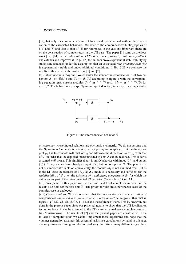
[18], but only for commutative rings of functional operators and without the specifi-cation of the associated behaviors. We refer to the comprehensive bibliographies of[17] and [5] and also to that of [4] for references to the vast and important literatureon the construction of compensators in the LTI case. The paper [1] sums up previouswork [19], [14] on the stabilization of LTV state space systems by static state feedbackand extends and improves it. In [2, §5] the authors prove exponential stabilizability bystatic state feedback under the assumption that an associated zero dynamics behavioris exponentially stable and under additional conditions. In Ex. 3.23 we compare theresults of this paper with results from [1] and [2].(vi) Interconnection diagram: We consider the standard interconnection B of two be-haviors B1 := B(U1) and B2 := B(U2) according to figure 1 with the correspond-ing equation resp. system modules Ui ⊆ A1×(p+m) resp. Mi = A1×(p+m)/Ui fori = 1, 2. The behaviors B1 resp. B2 are interpreted as the plant resp. the compensator

u1 r -u1 + y2

+- B1 -r y1

?ru2

r�y1 + u2

+�B2�r

y2

6r

Figure 1: The interconnected behavior B.

or controller whose mutual relations are obviously symmetric. We do not assume thatthe Bi are input/output (IO) behaviors with input ui and output yi. But the dimensionp of y1 has to coincide with that of u2 and likewise the dimension m of y2 with thatof u1 in order that the depicted interconnected system B can be realized. This latter isassumed well-posed. This signifies that it is an IO behavior with input ( u2

u1) and output

( y1y2 ). So ui can be chosen freely as input of B, but not as input of Bi. The plant B1 isnot assumed controllable or, equivalently, the module M1 is not assumed free. But asin the LTI case the freeness of M1,S as AS-module is necessary and sufficient for thestabilizability of B1, i.e., the existence of a stabilizing compensator B2 for which theautonomous part of the interconnected IO behavior B is stable, cf. Cor. 3.11.(vii) Base field: In this paper we use the base field C of complex numbers, but theresults also hold for the real field R. The proofs for this are either special cases of thecomplex case or analogous.(viii) Generalizations: We are convinced that the construction and parametrization ofcompensators can be extended to more general interconnection diagrams than that infigure 1, cf. [22, Ch. 5], [5, Ch. 11 ], [3] and the references there. This is, however, notdone in the present paper since our principal goal is to show that the LTI localizationtechnique from [4] can be extended to the LTV case with analogous complete results.(ix) Constructivity: The results of [7] and the present paper are constructive. Dueto lack of computer skills we cannot implement these algorithms and hope that theyounger generation assumes this essential task since calculations by hand in this areaare very time-consuming and do not lead very far. Since many different algorithms

2 DIFFERENTIAL OPERATORS AND BEHAVIORS 4

from the literature, for instance from [15], [10] and [20], have to be combined this im-plementation will not be easy.(x) Plan: The main theorems of this paper are proven in Section 4. Thm. 3.14 es-tablishes the Kucera-Youla parametrization for the LTV case and is the main result ofSection 3. Section 2 recalls the basic notions and results from the paper [7]. We illus-trate the construction and parametrization of all tracking stabilizing compensators inExamples 3.19 and 4.5.Notations and abbreviations: f.d.=finite-dimensional, f.g.=finitely generated,IO=input/output, LTI=linear time-invariant, LTV=linear time-varying, p.g.f.= polyno-mial growth function, resp.=respectively, w.e.s.= weak exponential stability, weaklyexponentially stable, w.l.o.g.=without loss of generality, Xp×q=set of p × q-matriceswith entries in X , X1×q=rows, Xq := Xq×1=columns , X•×• :=

⋃p,q≥0X

p×q .

2 Differential operators and behaviors

2.1 Differential operatorsThe differential operators and behaviors of this paper and their properties were in-troduced and discussed in [7]. We recapitulate them here and refer to [7, §§3,4] fordetails and references to the literature.The signals of this paper are defined on open real intervals (τ,∞), τ ≥ 0. Since westudy the trajectories for t → ∞ the restriction to τ ≥ 0 is no loss of generality. Theused signal spaces are the spaces of complex-valued smooth functions or distributionson (τ,∞), τ ≥ 0, i.e.,

W (τ) = C∞(τ,∞) or W (τ) = D′(τ,∞). (1)

The valued differential field of formal Laurent series with its valuation v : C((z)) →Q ] {∞} and derivation d/dz : C((z))→ C((z)) is given by

C((z)) :=

{a =

∞∑i=k

aizi; k ∈ Z, ai ∈ C

}with

v(a) :=

{k if ak 6= 0

∞ if a = 0, da/dz := a′(z) :=

∞∑i=k

aiizi−1.

(2)

The field C((z)) has the valued differential subfield of locally convergent Laurent seriesgiven by

C << z >>:=

{a =

∞∑i=k

aizi ∈ C((z)); σ(a) := lim sup

i≥0

i√|ai| <∞

}(3)

The inverse ρ(a) := σ(a)−1 is the convergence radius of a, i.e., a(z) =∑∞i=k aiz

i

converges for 0 < |z| < ρ(a) and is a holomorphic function in this pointed open disc.Therefore the function a(t−1) is contained in C∞(σ(a),∞).The valued differential field K is defined as the field of Puiseux series

K :=⋃m≥1

C << z1/m >>=

{a(z1/m) =

∞∑i=k

aizi/m; m ∈ N, m ≥ 1, k ∈ Z, a =

∞∑i=k

aizi ∈ C << z >>

}.

(4)


This field K is the algebraic closure of C << z >> and is constructed algebraicallysuch that

(z1/n

)n/m= z1/m if m divides n. The element z1/m is not defined as

the function exp(m−1 ln(z)) since ln(z) is not a Laurent series at 0. The valuationv is extended to K by v

(a(z1/m)

)= v(a)/m ∈ Q ] {∞} and the derivation by

da(z1/m)/dz = m−1z(1/m)−1a′(z1/m). We also define σ(a(z1/m)) := σ(a)m. Thefield K has the differential subalgebras

K(τ) :={f = a(z1/m) ∈ K; τ ≥ σ(f) = σ(a)m

}with

K(τ0) ⊆ K(τ) for τ0 ≤ τ and K =⋃τ≥0

K(τ).(5)

Iff = a(z1/m) ∈ K(τ) and t > τ then t > τ ≥ σ(f) = σ(a)m =⇒t−1/m < ρ(a) = σ(a)−1 =⇒ f(t) := a(t−1/m) ∈ C∞(τ,∞),

(6)

especially f(t) ∈ C∞(σ(f),∞). The map

K(τ)→ C∞(τ,∞), f = a(z1/m) 7→ f(t) := a(t−1/m), (7)

is an injective algebra homomorphism. The differential field K gives rise to the skew-polynomial ring of differential operators

A = K[∂; d/dz] = ⊕∞j=0K∂j . (8)

The differential operators are polynomials in ∂ whose noncommutative multiplicationis determined by

∂a(z1/m) = a(z1/m)∂ +m−1z(1/m)−1a′(z1/m). (9)

The ring A is a left and right principal ideal domain, indeed admits euclidean division,and is simple. For any nonzero h ∈ K the indeterminate ∂ can be replaced by h∂ andthe derivation by hd/dz and one obtains

A = K[h∂;hd/dz], especially A = K[z∂; zd/dz] = K[−z2∂;−z2d/dz]. (10)

The domain A has the subdomains

A(τ) := K(τ)[∂; d/dz] = K(τ)[z∂; zd/dz] = K(τ)[−z2∂;−z2d/dz] with

A(τ0) ⊆ A(τ) for 0 ≤ τ0 ≤ τ and A =⋃τ≥0

A(τ). (11)

We extend the function σ to differential operators and matrices via

σ(f) := max {σ(fj); j ∈ N) for f =∑j∈N

fj∂j ∈ A where

fj = aj(z1/m), σ(fj) = σ(aj)

m

σ(R) := max {σ(Rµν); µ ≤ p, ν ≤ q} for R = (Rµν)µ,ν ∈ Ap×q. Then

f ∈ A(τ) ⇐⇒ τ ≥ σ(f) and R ∈ A(τ)p×q ⇐⇒ τ ≥ σ(R).

(12)


The signal spaces W (τ0), τ0 ≥ 0, from (1) are not A-modules, but A(τ0)-leftmodules via the action f ◦ w, defined by ∞∑

j∈Nfj(−z2∂)j

◦ w :=∑j∈N

fj(t)w(j),

wherefj = aj(z1/m) ∈ K(τ0), fj(t) = aj

(t−1/m

)a(z1/m) ◦ w = a(t−1/m)w, (−z2∂) ◦ w = w′ := dw/dt, ∂ ◦ w = −t2w′.

(13)

Notice that there is no module action (=scalar multiplication) ◦′ with a(z1/m) ◦′ w =a(t−1/m)w and ∂ ◦′ w = w′. As usual the action (13) is extended to the action R ◦ wof a matrix R ∈ A(τ0)

p×q on a column vector w ∈W (τ0)q and defined by

R ◦ w =∑j∈N

Rj(t)w(j) for R =

∑j∈N

Rj(−z2∂)j ∈ A(τ0)p×q

where Rj = Aj(z1/m) ∈ K(τ0)

p×q, i.e., τ0 ≥ σ(Rj), Aj ∈ C << z >>p×q,

Rj(t) = Aj(t−1/m) ∈ C∞(τ,∞)p×q.

(14)Any matrix R =

∑j∈NRj(−z2∂)j ∈ Ap×q gives rise to the solution spaces or be-

haviors B(R, τ), τ ≥ σ(R), defined by

B(R, τ) := {w ∈W (τ)q; R ◦ w = 0} =

w ∈W (τ)q;∑j∈N

Rj(t)w(j) = 0

.

(15)The dependence of the admissible τ on the matrix R requires a new definition of be-haviors that is explained in Section 2.2.

2.2 Modules and behaviorsWe assume the data of Section 2.1 and consider matrices R ∈ Ap×q and associ-ated behavior families from (15): (B(R, τ))τ≥τ0 , τ0 ≥ σ(R). Two such families(B(Ri, τ))τ≥τi , i = 1, 2, are called equivalent if

∃τ3 ≥ max(τ1, τ2)∀τ ≥ τ3 : B(R1, τ) = B(R2, τ). (16)

The equivalence class is denoted by cl ((B(R, τ))τ≥τ0), hence especially

cl ((B(R, τ))τ≥τ0) = cl((B(R, τ))τ≥σ(R)

). (17)

For R = 0 ∈ A1×q one especially obtains the classes

W := cl ((W (τ))τ≥0) andWq = cl ((W (τ)q)τ≥0) . (18)

These replace the standard signal modules in the following behavior theory.Let AModfg denote the category of f.g. A-left modules M with a given system ofgenerators or, equivalently, a given representation M = A1×q/U, U ⊆ A1×q . Themorphisms of the category are the A-linear maps without any additional structure. Thecategory is abelian.If M = A1×q/U ∈ AModfg the submodule U is f.g. and therefore the row module

3 KUCERA-YOULA PARAMETRIZATION FOR LTV SYSTEMS 7

U = A1×pR of some nonunique R ∈ A•×q that gives rise to cl((B(R, τ))τ≥σ(R)

).

This class does not depend on the choice of R and is called the behavior B(U) ⊆ Wq

of U or M [7, Lemma 3.7]. There is a naturally defined abelian category Beh ofbehaviors [7, Cor. and Def. 3.9] whose objects are the B(U), U ⊆ A1×q, q ≥ 0,and that enables a module-behavior duality. This signifies that there is a contravariantequivalence or duality [7, Thm. 2.2, Cor. 3.14]

AModfg ∼= Beh{M = A1×q/U 7→ B(U)

HomA(A1×q1/U1,A1×q2/U2) ∼= Hom(B(U2),B(U1)), ϕ 7→ B(ϕ).

(19)

Assume Ui = A1×piRi, Ri ∈ Api×qi . Every ϕ can be described as

ϕ = (◦P )ind : A1×q1/U1 → A1×q2/U2, ξ := ξ + U1 7→ ξP := ξP + U2,

where P ∈ Aq1×q2 , U1P ⊆ U2, ξ ∈ A1×q1 , ξP ∈ A1×q2 .(20)

In particular, there is an X ∈ Aq1×p2 with R1P = XR2. The morphism B(ϕ) isdefined as the equivalence class of C-linear maps

B(ϕ) = cl((P◦ : B(R2, τ)→ B(R1, τ), w2 7→ P ◦ w2)τ≥τ0

),

where τ0 ≥ max (σ(R1), σ(R2), σ(P ), σ(X)) .(21)

The equivalence class is defined analogously to that in (17) [7, §3.3]. So objects andmorphisms in Beh are given by the behaviors

B(Ri, τ), i = 1, 2, and maps P◦ : B(R2, τ)→ B(R1, τ), τ ≥ τ0, (22)

for sufficiently large τ0. The module M = A1×q/U with U = A1×pR, R ∈ Ap×q,is a torsion module or, equivalently, rank(R) = q if and only if B(U) is autonomous.Autonomy signifies that there are τ1 ≥ σ(R) and d ∈ N such that for all t0 > τ ≥ τ1the initial map

B(R, τ)→ Cdq, w 7→ (w(t0), · · · , w(d−1)(t0))>, is injective. (23)

A function ϕ : [τ0,∞)→ C, τ ≥ 0, is called p.g.f. if it grows at most polynomially fort→∞. All functions f(t) for f ∈ K are p.g.f. on each closed interval [τ0,∞), τ0 >σ(f). The autonomous behavior B(U), is called weakly exponentially stable (w.e.s.)[7, Def. 2.3] if there are τ1 ≥ σ(R), d ∈ N, α, µ > 0 and, for each m ∈ N, a p.g.f.ϕm(t) > 0 on [τ1,∞) such that all trajectories w ∈ B(R, τ), τ ≥ τ1, satisfy theinequalities

‖w(m)(t)‖ ≤ ϕm(t0) exp (−α(tµ − tµ0 )) ‖x(t0)‖ for t ≥ t0 > τ where

x(t0) := max(‖w(t0)‖, ‖w′(t0)‖, · · · , ‖wd−1(t0)‖).(24)

3 Kucera-Youla parametrization for LTV systems

3.1 Weakly exponentially stable localizationSince A is a (left and right) noetherian domain the set A \ {0} is an Ore set and givesrise to the quotient field of A [13, Thm. 2.1.15]:

Q := quot(A) := (A \ {0})−1 A ={s−1a = bt−1; a, b, s, t ∈ A, s 6= 0, t 6= 0

}.

(25)


Lemma 3.1. Each nonzero ideal is essential or large in A or, in other words, if theelements ai, i = 1, 2, are nonzero then also Aa1

⋂Aa2 6= 0.

Proof. There are b1, b2 such that a1a−12 = b−11 b2, hence 0 6= b1a1 = b2a2 ∈ Aa1⋂Aa2.

Since the f.g. w.e.s. modules form a Serre category the same holds true for the fullsubcategory C of the category AMod of all left A-modules whose f.g. submodulesare w.e.s.. Moreover, if Ci, i ∈ I, are, possibly infinitely many, submodules in C of aleft A-module M then also the sum C :=

∑i∈I Ci belongs to C. In particular, each

AM has a largest submodule RaC(M) in C that is called the C-radical of M . We alsoconsider the set

S := {s ∈ A; A/As w.e.s. or A/As ∈ C} . (26)

of all w.e.s. differential operators.In the sequel we call the modules in C and the elements in S just stable instead of w.e.s..No other stability notion will be used.

Corollary 3.2. ([7, Cor. 4.16]) If 0 6= s = s1s2 ∈ A then s ∈ S if and only ifs1, s2 ∈ S. In other words, S is multiplicatively closed and saturated.

Lemma 3.3. The set S is an Ore set, i.e., for b ∈ A and t ∈ S there are a ∈ A ands ∈ T with sb = at or bt−1 = s−1a ∈ Q.

Proof. Consider the linear map α : A → A, x 7→ xb and a := α−1(At) = As. Themap induces the injection αind : A/a → A/At ∈ C, hence A/a ∈ C and s ∈ S. Bydefinition α(s) = sb ∈ At and therefore there is an a ∈ A with sb = at.

The Ore set S gives rise to the quotient ring S−1A = AS ⊂ Q and to the AS-quotient module S−1M = MS of an A-left module M [13, §2.1]. They have theform

A ⊂ S−1A := AS :={s−1a = bt−1; a, b ∈ A, s, t ∈ S, at = sb

}⊂ Q := quot(A)

S−1M :=MS :={s−1x =

x

s; x ∈M, s ∈ S

}.

(27)There is also the canonical A-linear map [13, Prop. 2.1.17]

canM :M →MS , x 7→x

1, with kernel

torS(M) := ker(canM ) = {x ∈M ; ∃s ∈ S with sx = 0} ⊆ tor(M).(28)

Here tor(M) resp. torS(M) are the torsion resp. S-torsion submodules of M . Asusual the assignment M 7→MS is extended to the exact quotient functor

AMod→ ASMod,

{M 7→MS

(ϕ :M1 →M2) 7→(S−1ϕ = ϕS : M1,S →M2,S

)where ϕS

(x1s

):=

ϕ(x1)

s.

(29)For an A-(left) module M , x ∈ M and annihilator left ideal As = annA(x) :={a ∈ A; ax = 0} the map A/As ∼= Ax, a + As 7→ ax, is an isomorphism. Itimplies that

s ∈ S ⇐⇒ A/As ∈ C ⇐⇒ Ax ∈ C ⇐⇒ x ∈ RaC(M). (30)


Corollary 3.4. The torsion submodule torS(M) of M is the largest submodule of Min C, i.e., torS(M) = RaC(M), especially

M ∈ C ⇐⇒ torS(M) =M ⇐⇒ MS = 0. (31)

Notice that A is simple and hence the two-sided annihilator ideal annA(M) ={a ∈ A; aM = 0} is zero if M is nonzero.

Lemma 3.5. Like A itself the quotient ring AS ⊂ Q = quot(A) is a left and rightprincipal ideal domain and simple.

Proof. 1. Any left ideal b ⊆ AS satisfies b = (A⋂b)S = AS(A

⋂b). But A

⋂b is

principal and hence A⋂b = Aa and b = ASa.

2. If b ⊆ AS is a nonzero two-sided ideal of AS then so is a := A⋂

b of A. Since Ais simple a = A and hence also b = AS .

3.2 Stable input/output behaviorsConsider a behavior B := B(U) for some U ⊆ A1×q and M = A1×q/U . Recall thatU is a free submodule of A1×q . Then

QU = Q⊗A U ⊆ Q1×q = Q⊗A A1×q and Q⊗A M =identification

Q1×q/QU. (32)

As usual we define

p := rank(U) := dimA(U) = dimQ (QU) ,

m := rank(M) := dimQ (Q⊗A M) , hence p+m=q

=⇒ ∃R ∈ Ap×q with rank(R) = p, U = A1×pR.

(33)

In general there are various subsets I ⊂ {1, · · · , q} of p elements such that the pro-jection proj : Q1×q → Q1×I induces an isomorphism proj : QU ∼= Q1×I . Such asubset I is called an input/output (IO) structure of U , M or B and B with this structureis called an IO behavior. We assume such a structure and also as usual, after a possiblecolumn permutation, that I = {1, · · · , p} and hence the isomorphism

Q1×(p+m) ⊃ QU ∼= Q1×p, (ξ, η) 7→ ξ. (34)

This isomorphism, in turn, is equivalent to the isomorphism

(◦(0, idm))ind : Q1×m ∼= Q1×(p+m)/QU = Q⊗A M, η 7→ (0, η) +QU. (35)

With U0 = U(idp

0

)⊆ A1×p and M0 := A1×p/U0 the preceding isomorphisms are

also equivalent to rank(M0) = 0, i..e., the torsion property of M0, and the exactnessof

0→ A1×m (◦(0,idm))ind−→ M = A1×(p+m)/U

(◦(idp

0

))ind−→ M0 = A1×p/U0 → 0.

(36)For the matrix R the isomorphisms (34) and (35) imply

R = (P,−Q) ∈ Ap×(p+m), p = rank(R) = rank(P ), H = P−1Q,

U = A1×p(P,−Q) ⊆ A1×(p+m), U0 = A1×pP ⊆ A1×p.(37)


Here we used the equivalences

rank(P ) = p ⇐⇒ Q1×pP = Q1×p ⇐⇒ PQp = Qp ⇐⇒ P ∈ Glp(Q). (38)

The matrix H is the transfer matrix of the IO behavior. It is also characterized by theproperty that

QU = Q1×p(P,−Q) = Q1×p(idp,−H). (39)

This shows that H depends on U and the IO structure, but not on the special choiceof R. Recall the behaviorW := cl ((W (τ))τ≥0). By duality the exactness of (36) isequivalent to the exactness of the behavior sequences

0→ B(U0)

(idp

0

)◦

−→ B(U)(0,idm)◦−→ W1×m → 0

0→ B(P, τ)

(idp

0

)◦

−→ B((P,−Q), τ)(0,idm)◦−→ W (τ)m → 0

y 7→ ( y0 ) , (yu ) 7→ u

B(P, τ) = {y ∈W (τ)p; P ◦ y = 0} ,B((P,−Q), τ) =

{( yu ) ∈W (τ)p+m; P ◦ y = Q ◦ u

},

(40)

where τ ≥ τ0 and τ0 ≥ 0 is sufficiently large.

Lemma and Definition 3.6. For the IO behavior B = B(U) from above and its au-tonomous part B0 = B(U0) the following properties are equivalent:1. The autonomous behavior B0 or M0 are stable, i.e., M0

S = 0 or A1×pS P = A1×p

S

or P ∈ Glp(AS).2. The quotient module MS is free and H ∈ Ap×m

S .If 1. and 2. are satisfied the IO behavior is called weakly exponentially stable (w.e.s.)or just stable.

Proof. 1. =⇒ 2.: The stability of M0 implies M0S = 0. We apply the exact quotient

functor M 7→MS to (36) and infer the isomorphism A1×mS

∼=MS , hence MS is free.Moreover P ∈ Glp(AS) and hence H = P−1Q ∈ Ap×m

S .2. =⇒ 1.: Application of the exact quotient functor (−)S to the exact sequence

0→ A1×p ◦(P,−Q)−→ A1×(p+m) can−→M = A1×(p+m)/A1×p(P,−Q)→ 0 (41)

with the canonical map can furnishes the exact sequence of AS-modules

0→ A1×pS

◦(P,−Q)−→ A1×(p+m)S

can−→MS → 0. (42)

Since MS is free this sequence splits and in particular (P,−Q) has a right inverse(XY ) with X,Y ∈ A•×•S and idp = ( P −Q ) (XY ) = PX − QY = P (X − HY ).Since H ∈ A•×•S the last equation implies that P has the right inverse and thus inverseX −HY , i.e., P ∈ Glp(AS).

3.3 Stabilizing compensatorsWe consider the interconnected behavior B of the plant B1 and the controller B2 ac-cording to figure 1. The components of B1 resp. B2 are

( y1u1) , ( u2

y2 ) ∈W (τ)p+m. (43)


In the interconnected behavior B the component yi is added to the component u3−i fori = 1, 2. The behaviors are given as

B1 = B(U1), U1 = A1×pR1, R1 ∈ Ap×(p+m), dimA(U1) = rank(R1) = p

B2 = B(U2), U2 = A1×mR2, R2 ∈ Am×(p+m), dimA(U2) = rank(R2) = m

M1 := A1×(p+m)/U1, M2 := A1×(p+m)/U2.(44)

As indicated in the Introduction we neither assume that the behaviors Bi, i = 1, 2,are IO behaviors with inputs ui nor that they are controllable (cf. [5, §11.2, p.545]).Nevertheless we decompose the matrices Ri as

R1 = (P1,−Q1) ∈ Ap×(p+m), R2 = (−Q2, P2) ∈ Am×(p+m), hence

B(R1, τ) ={( y1u1

) ∈W (τ)p+m; P1 ◦ y1 = Q1 ◦ u1},

B(R2, τ) ={( u2y2 ) ∈W (τ)p+m; P2 ◦ y2 = Q2 ◦ u2

},

B(U1) = cl ((B(R1, τ))τ≥τ0) , B(U2) = cl ((B(R2, τ))τ≥τ0) , τ ≥ τ0,

(45)

where, as usual, τ0 is sufficiently large. The interconnected behavior B is then definedby

B = cl ((B(τ))τ≥τ0) , B(τ) ={( yu ) ∈W (τ)(p+m)+(p+m); P ◦ y = Q ◦ u

}where

y = ( y1y2 ) ∈W (τ)p+m, u = ( u2u1

) ∈W (τ)p+m,

{P1 ◦ y1 = Q1 ◦ (u1 + y2)

P2 ◦ y2 = Q2 ◦ (u2 + y1)

P :=(R1

R2

)=(

P1 −Q1

−Q2 P2

)∈ A(p+m)×(p+m), Q :=

(0 Q1

Q2 0

)∈ A(p+m)×(p+m).

(46)The corresponding modules are

U := A1×(p+m)(P,−Q) ⊆ A1×2(p+m), M := A1×2(p+m)/U, B := B(U),

U0 := A1×(p+m)P = A1×pR1 +A1×mR2 = U1 + U2 ⊆ A1×(p+m),

M0 := A1×(p+m)/U0, B0 := B(U0),

rank(P ) = dimA(U0) = dimA(U1 + U2) ≤ dimA(U1) + dimA(U2) = p+m.(47)

Lemma and Definition 3.7. (Cf. [5, Thm. and Def. 1136, p.546]) Assume the datafrom (44)-(47). The following properties are equivalent:

1. rank(P ) = p +m or, equivalently, P ∈ Glp+m(Q), i.e., B is an IO behaviorwith input u = ( u2

u1) and output y = ( y1y2 ).

2. U0 = U1 ⊕ U2 or, equivalently, U1

⋂U2 = 0.

If these conditions are satisfied the behavior B is called well-posed, its autonomouspart is B0 = B(U0) and its transfer matrix is H = P−1Q.

Proof. dimA(U1 + U2) = dimA(U1) + dimA(U2) ⇐⇒ U1

⋂U2 = 0.

Remark 3.8. In the following theory the behavior B is always assumed well-posedor, equivalently, an IO behavior with input ( u2

u1). Since all considerations refer to the

interconnected behavior B the components u1 and u2 are free (can be freely chosen)


as inputs of B although they are not free in general as inputs of B1 resp. B2. Transfermatrices H1, H2 and their usual factorizations H1 = P−11 Q1 and H2 = P−12 Q2 donot exist in general and are not needed or used in the following.

Corollary and Definition 3.9. For the behavior B from (46) and (47) the followingproperties are equivalent:

1. P ∈ Glp+m(AS).

2. The interconnected behavior B is well-posed, MS is AS-free, necessarily ofdimension p+m, and H = P−1Q ∈ A

(p+m)×(p+m)S .

3. U1,S ⊕ U2,S = A1×(p+m)S .

These equivalent properties imply the canonical isomorphisms

M1,S∼= A

1×(p+m)S /U1,S

∼= U2,S (48)

and thus that M1,S is a free AS-module of dimension m = rank(M1). The behaviorB2 is then called a weakly exponentially stabilizing or just a stabilizing compensatorof B1. Obviously this property holds reciprocally, i.e., B1 is also a stabilizing compen-sator for B2.

Proof. 1. ⇐⇒ 2.: Lemma and Def. 3.6.In 2. and 3. the well-posedness of the feedback behavior implies

U = U1 ⊕ U2 = A1×(p+m)P and US = U1,S ⊕ U2,S = A1×(p+m)S P.

1. ⇐⇒ 3.:

P ∈ Glp+m(AS) ⇐⇒ A1×(p+m)S P = A

1×(p+m)S ⇐⇒ U1,S ⊕ U2,S = A

1×(p+m)S .

Definition 3.10. The behavior B(U1) or module M1 are called weakly exponentiallystabilizable or just stabilizable if B(U1) admits a stabilizing compensator B(U2) ac-cording to Cor. and Def. 3.9.

Corollary 3.11. The behavior B1 from (43) is stabilizable if and only if M1,S is a freeAS-module, necessarily of dimension m.

Proof. 1. If B1 is stabilizable then M1,S is free according to Cor. and Def. 3.9 and(48). If, conversely, M1,S is free the canonical map can : A

1×(p+m)S → M1,S =

A1×(p+m)S /U1,S has a section or right inverse σ and hence

A1×(p+m)S = ker(can)⊕ im(σ), U1,S ⊕ V, V := im(σ).

Define

U2 := A1×(p+m)⋂V, hence V = U2,S and A

1×(p+m)S = U1,S ⊕ U2,S . Then

dimA(U2) = dimAS(U2,S) = (p+m)− dimAS

(U1,S) = (p+m)− p = m.

Equation (44) and Cor. and Def. 3.9 imply that B2 := B(U2) is a stabilizing compen-sator of B1.


3.4 The parametrization of stabilizing compensatorsThis section contains the LTV version of the Kucera-Youla parametrization for themodules and behaviors of this paper. Assume that the behavior B1 from (44) is stabi-lizable, i.e., that M1,S

∼= A1×mS . Omission of M1,S in the exact sequence

0→ A1×pS

◦(P1,−Q1)−→ A1×(p+m)S

can−→M1,S∼= A1×m

S → 0

furnishes a split exact sequence

0→ A1×pS

◦(P1,−Q1)−→ A1×(p+m)S

◦(N1

D1

)−→ A1×m

S → 0 where(N1

D1

)∈ A

(p+m)×mS .

(49)Since the sequence splits the matrix (P1,−Q1) has a right inverse

(D0

2

N02

)∈ A

(p+m)×pS

and(N1

D1

)has a left inverse (−Q0

2, P02 ) ∈ A

m×(p+m)S such that also the sequence

0← A1×pS

◦(D0

2

N02

)←− A

1×(p+m)S

(−Q02,P

02 )←− A1×m

S ← 0(50)

is exact. This is a standard algebraic result, cf. [4, Lemma 2.3]. Moreover

A1×(p+m)S = A1×p

S (P1,−Q1)⊕A1×mS (−Q0

2, P02 )

E01 :=

(D0

2

N02

)(P1,−Q1) = (E0

1)2, E0

2 =(N1

D1

)(−Q0

2, P02 ) = (E0

2)2,

idp+m =(

idp 00 idm

)= E1 + E2 =

(D0

2P1−N1Q02, −D

02Q1+N1P

02

N02P1−D1Q

02, −N

02Q1+D1P

02

)=(D0

2 N1

N02 D1

)(P1 −Q1

−Q02 P 0

2

)=⇒

(P1 −Q1

−Q02 P 0

2

)−1=(D0

2 N1

N02 D1

).

(51)

The parametrization of all sequences (50) or, equivalently, all V ⊆ A1×(p+m) withU1,S ⊕ V = A

1×(p+m)S is the analogue of the Kucera-Youla parametrization that was

established in the LTI case only. The following lemma is the LTV form of this. Itsproof is a standard result on split exact sequences and analogous to that of [4, Lemma3.10].

Lemma 3.12. (Cf. [4, Lemma 3.10]) Assume that the behavior B(U1) from (44) isstabilizable and the ensuing exact sequences (49) and (50).1. The following bijections hold:{

V ⊆ A1×`S ; U1,S ⊕ V = A

1×(p+m)S

}3 V

∼= l{(D2

N2

); (P1,−Q1)

(D2

N2

)= idp

}3

(D2

N2

)∼= l{

(−Q2, P2) ∈ Am×(p+m)S ; (−Q2, P2)

(N1

D1

)= idm

}3 (−Q2, P2)

∼= lAm×p 3 X

(52)

The bijections are given by the equations

V = ker(◦(D2

N2

))= A1×m

S (−Q2, P2),(D2

N2

)=(D0

2

N02

)−(N1

D1

)X

(−Q2, P2) = (−Q02, P

02 ) +X(P1,−Q1), P2 = P 0

2 −XQ1, Q2 = Q02 −XP1.

(53)


2. In analogy to (50) and (51) these data give rise to the exact sequence

0← A1×pS

◦(D2

N2

)←− A

1×(p+m)S

(−Q2,P2)←− A1×mS ← 0 and to(

P1 −Q1

−Q2 P2

)−1=(D2 N1

N2 D1

),

H =(Hy1,u2 Hy1,u1

Hy2,u2Hy2,u1

)=(

P1 −Q1

−Q2 P2

)−1 (0 Q1

Q2 0

)=(N1Q2 D2Q1

D1Q2 N2Q1

).

(54)

Corollary 3.13. According to Cor. and Def. 3.9 every stabilizing compensator B(U2)

of B(U1) gives rise to a decompositionU1,S⊕U2,S = A1×(p+m)S . According to Lemma

3.12 U2,S has a unique representation U2,S = A1×mS (−Q2, P2) where (−Q2, P2) ∈

Am×(p+m)S is precisely one matrix as described in the lemma.

Theorem 3.14. (Construction of all stabilizing compensators) Assume that the behav-ior B(U1) from (44) is stabilizable and the ensuing exact sequences (49), (50) and datafrom Lemma 3.12. All stabilizing compensators B(U2) of B(U1) are obtained in thefollowing fashion:

(i) Choose a direct complement V = A1×mS (−Q2, P2) ofU1,S according to Lemma

3.12 and define the matrix RV2 = (−QV2 , PV2 ) ∈ Am×(p+m) by

A1×mRV2 = UV2 := A1×(p+m)⋂V, hence A1×m

S RV2 = UV2,S = V. (55)

In other words, the rows of RV2 are an AS-basis of V in A1×m.

(ii) Choose a matrix Y ∈ Am×m⋂Glm(AS) (cf. Remark 3.15) and define

RA2 := Y RV2 = (−QA

2 , PA2 ) and U2 := A1×mRA

2 . (56)

For given V the unique controllable compensator is B(UV2 ).

Proof. 1. The constructed B(U2) is a stabilizing compensator: Since Y ∈ Glm(AS)we get

U2,S = A1×mS Y RV2 = A1×m

S RV2 = V and dimA(U2) = dimAS(V ) = m.

2. Every stabilizing compensator has this form: Let U2 be the equation module of astabilizing compensator B(U2). We define V := U2,S and obtain, by Cor. and Def.3.9, U1,S ⊕ V = A

1×(p+m)S . Thus V is a submodule as in item (i). Moreover

U2 ⊆ A1×(p+m)⋂V = A1×mRV2 , hence ∃Y ∈ Am×m such that

U2 = A1×mY RV2 and A1×mS RV2 = V = U2,S = A1×m

S Y RV2 .

Since rank(RV2 ) = m the rows of RV2 are Q-linearly independent and RV2 can be can-celled as right factor. We conclude A1×m

S Y = A1×mS and Y ∈ Am×m⋂Glm(AS).

3. (i) The inclusion

MV2 := A1×(p+m)/

(A1×(p+m)

⋂V)⊂

ident.A

1×(p+m)S /V

implies that MV2 is torsionfree and thus free and hence B(UV2 ) is controllable.

(ii) If, conversely, B(U2) is controllable and M2 = A1×(p+m)/U2 is free and hencetorsionfree then the canonical map M2 → M2,S = A

1×(p+m)S /U2,S = A

1×(p+m)S /V

is injective. This signifies that U2 = A1×(p+m)⋂V = UV2 .


Remark 3.15. (Cf. [11, Cor. 1.4.8], [5, Thm. and Def. 662]) Every matrix Y ∈

Am×m is equivalent to a diagonal matrix D = diag(11, · · · , 1, ra, 0, · · · ,

m0) ∈ Am×m

where 0 ≤ r ≤ m and a 6= 0. Then r = rank(Y ) and, of course, r = m if andonly if Y ∈ Glm(Q). The matrix Y can be obtained from D by a finite sequence ofelementary row and column operations. This implies

Y ∈ Am×m⋂

Glm(AS) ⇐⇒ D ∈ Am×m⋂

Glm(AS) ⇐⇒ r = m and a ∈ S.(57)

Hence all matrices Y ∈ Am×m⋂Glm(AS) in Thm. 3.14 can be obtained from diag-onal matrices D = diag(1, · · · , 1,ms ), s ∈ S, by a sequence of elementary row andcolumn operations.

We specialize the preceding considerations to a controllable IO behavior B1. Forthis purpose assume an arbitrary nonzero transfer matrix H1 ∈ Qp×m. The matrices(H1

idm

)resp. (− idp, H1) have rank m resp. p and thus give rise to exact sequences

0→ A1×p ◦(P1,−Q1)−→ A1×(p+m)◦(H1

idm

)−→ Q1×m

0→ Am

(N1

D1

)◦

−→ Ap+m (− idp,H1)◦−→ Qp

,

=⇒

{P1H1 = Q1, rank(P1) = rank(P1,−Q1) = p, P1 ∈ Glp(Q), H1 = P−11 Q1

H1D1 = N1, rank(D1) = rank(N1

D1

)= m, D1 ∈ Glm(Q), H1 = N1D

−11

.

(58)Since Q1×m and Qp are A-torsionfree the modules

M1 := A1×(p+m)/U1, U1 := A1×p(P1,−Q1), and Ap+m/(N1

D1

)Am (59)

are left resp. right A-free. In particular, B1 := B(U1) is controllable and an IObehavior due to P1 ∈ Glp(Q) and the matrices (P1,−Q1) resp.

(N1

D1

)have a right

inverse resp. a left inverse. The exactness of (58) implies that of (49) with AS replacedby A, i.e., of

0→ A1×p ◦(P1,−Q1)−→ A1×(p+m)◦(N1

D1

)−→ A1×m → 0

(60)

The matrices P1 resp. D1 are unique up to multiplication with a matrix of Glp(A)resp. Glm(A) from the left resp. the right. By Lemma and Def. 3.6 the controllable IObehavior B1 is stable or P1 ∈ Glp(AS) if and only if H1 ∈ Ap×m

S . With an analogousargument one proves

Corollary 3.16. (Cf. [5, Prop. 1012]) The following properties are equivalent for thecontrollable behavior B1 = B(A1×p(P1,−Q1)) from (58)-(60):

B1 is stable ⇐⇒ H1 ∈ Ap×mS ⇐⇒ P1 ∈ Glp(AS) ⇐⇒ D1 ∈ Glm(AS). (61)

Proof. Only the last equivalence has still to be shown. Obviously

D1 ∈ Glm(AS) =⇒ H1 = N1D−11 ∈ Ap×m

S .

If, conversely, H1 belongs to Ap×mS localization of the second exact sequence of (58)

furnishes the exact sequence

0→ AmS

(N1

D1

)◦

−→ Ap+mS

(− idp,H1)◦−→ ApS → 0. But ker ((− idp, H1)◦) =

(H1

idm

)AmS

=⇒ ∃X ∈ Glm(AS) with(N1

D1

)=(H1

idm

)X =⇒ D1 = X ∈ Glm(AS).


The last equivalence of Cor. 3.16 also follows from the isomorphism

(◦N1)ind : A1×p/A1×pP1∼= A1×m/A1×mD1, (62)

cf. [5, Prop. 1012]. According to Lemma 3.12 there are a right inverse(D0

2

N02

)∈

Ap×(p+m) of (P1,−Q1) and a left inverse (−Q02, P

02 ) of

(N1

D1

)such that also

0← A1×p◦(D0

2

N02

)←− A1×(p+m) ◦(−Q0

2,P02 )←− A1×m ← 0

(63)

is exact. This is the exact sequence (50) with AS replaced by A. The behaviorB(A1×m(−Q0

2, P02 )) is one stabilizing compensator of B1. Since

(P1 −Q1

−Q02 P 0

2

)∈

Glp+m(A) the autonomous part of the interconnected behavior is not only stable, butzero.

Corollary 3.17. Lemma 3.12 and Thm. 3.14 are applicable to the exact sequences(60) and (63) for the controllable IO behavior B1 from (58)-(60). Hence all stabilizingcompensators for B1 are obtained by the two steps of Thm. 3.14.

It is presently not clear which P2 = P 02 −XQ1 belong to Glm(Q) and then make

the compensator an IO behavior.

Remark 3.18. Standard terminology: The behavior B1 is called the (unique) control-lable realization of the transfer matrix H1. The representations H1 = P−11 Q1 resp.H1 = N1D

−11 are the essentially unique left resp. right coprime factorizations of H1.

Example 3.19. This example is constructed without computer algebra from the desiredoutcome instead from a plant of engineering relevance. Consider the stable operators

s1 := −2z2∂ + z1/2, s2 := −z2∂ + 1 with the stable solutions

y1(t) = exp(−(t1/2 − t1/20 )

)y1(t0), y2(t) = exp (−(t− t0)) y2(t0), t ≥ t0 > 0

=⇒ s1, s2 ∈ S =⇒(s1 00 s2

)∈ Gl2(AS).

(64)We choose a ∈ A and define the matrices(

P1 −Q1

−Q02 P 0

2

):= ( 1 1

0 1 ) (1 0a 1 )

(s1 00 s2

)=((1+a)s1 s2as1 s2

)∈ Gl2(AS)(

D02 N1

N02 D1

):=(

P1 −Q1

−Q02 P 0

2

)−1=(s1 00 s2

)−1( 1 0a 1 )

−1( 1 10 1 )

−1

=(s−11 0

0 s−12

) (1 0−a 1

) (1 −10 1

)=(

s−11 −s−1

1

−s−12 a s−1

2 (a+1)

)∈ Gl2(AS).

(65)

Choose x ∈ AS arbitrarily and define

(−Q2, P2) := (−Q02, P

02 ) + x(P1,−Q1) = (as1, s2) + x((1 + a)s1, s2)

= ((1 + x)as1 + xs1, (1 + x)s2) ∈ A1×2S , x ∈ AS .

(66)

We conclude that

B1 := B (A((1 + a)s1, s2)) with B(((1 + a)s1, s2), τ)

={( y1u1

) ∈W (τ)2; (1 + a)s1 ◦ y1 = −s2 ◦ u1}, τ ≥ τ0,

(67)


is stabilizable where, as always, τ0 is sufficiently large. The behavior B1 is an IObehavior if and only if 1 + a 6= 0 and additionally stable if and only if 1 + a ∈ S. Theoperator 1 + a := 1 + z2∂ with its solution y(t) = exp(t− t0)y(t0) is not stable.The stabilizing compensators are obtained as follows: They are IO behaviors if andonly if 1 + x 6= 0. The parameter x 6= −1 has the form t−1b with arbitrary t ∈ S andb 6= −t in A. Since t ∈ S ⊂ Gl1(AS) we infer

AS(−Q2, P2) = ASt(−Q2, P2) = AS ((t+ b)as1 + bs1, (t+ b)s2)

= (A ((t+ b)as1 + bs1, (t+ b)s2))S(68)

According to Thm. 3.14 all stabilizing compensators of B1 have the form

B2 = B(Ar(−QA

2 , PA2 )), r ∈ S, where

A(−QA2 , P

A2 ) = A1×2

⋂AS ((t+ b)as1 + bs1, (t+ b)s2) , t ∈ S, −t 6= b ∈ A.

(69)The computation of (−QA

2 , PA2 ) by hand is difficult. Among these B2 there are the

compensators

B2 := B (A ((t+ b)as1 + bs1, (t+ b)s2)) with t ∈ S, −t 6= b ∈ A andB2 (((t+ b)as1 + bs1, (t+ b)s2) , τ)

={( u2y2 ) ∈W (τ)2; (t+ b)s2 ◦ y2 = −((t+ b)as1 + bs1) ◦ u2

}.

(70)

Remark 3.20. Comparison with [5, Thm. 1143, p. 554]: The Kucera-Youla parametriza-tion for differential LTV systems is also derived in the quoted theorem. The correspon-dence is given by

(AL,−BL) = (P1,−Q1),(BR

AR

)=(N1

D1

), (−RL, SL) = (−Q0

2, P02 ),(

SR

RR

)=(D0

2

N02

), (−Y ′, X ′) = (−Q2, P2), (XY ) =

(D2

N2

).

The signs differ slightly because the block diagram [5, Fig. 11.1] uses a minus sign atthe left upper node. The parameter matrixX from Lemma 3.12 corresponds toK = K.Nevertheless the quoted result differs from the derivations here. To point out the differ-ences the language of this paper is used: (i) The employed behaviors of [5] differ fromthose in [7] and the present paper. The differential field K is replaced by an Ore field[5, Lemma and Def. 835]. (ii) The behaviors B1 and B2 of [5, Fig. 11.1] are assumedas controllable IO behaviors. This signifies that the sequences (49) and (50) are exactwith AS replaced by A and that P1 ∈ Glp(Q) and P 0

2 ∈ Glm(Q). (iii) The quotedtheorem parametrizes the transfer matrices H from (54) and not the interconnectedbehaviors. (iv) The main difference consists in the notion of exponential stability [5,Thm. 998, Def. 1013], called bm-stability here. A torsion module A/AF is calledbm-stable if F is the product of linear factors z2∂+γ(t) with limt→∞<(γ(t)) < 0 [5,Thm. 998]. These linear operators are obviously stable. Such a product decompositiondoes not exist in general for F ∈ A and for Ore fields only very rarely as far as wesee. The same problem arises with the definition of a stable transfer matrix in [5, Def.1013]. Exactly these problems motivated the paper [7] with its general definition ofw.e.s. and its main result that permits to decide stability in most cases. (v) That thestable torsion modules form a Serre category implies that the set S of stable differentialoperators is an Ore set (cf. Lemma 3.3) and that the set AS of stable rational functionsis a (noncommutative) subring of Q. According to [22, p.3] this is the motivating prop-erty for the set of stable rational functions. This property is not shown for bm-stability


in [5], but the ensueing equivalence (61) is employed in [5, Prop. 1012, Def. 1013]and the third last line of the proof of [5, Thm. 1143]. It seems to us that the proof ofthe Kucera-Youla parametrization in [5] is incomplete.

3.5 State space representationsThe following state space representation of an arbitrary IO behavior is due to Fliesswith respect to its algebraic content. Its LTI analogue is Kalman’s famous realizationtheorem. We consider an IO behavior B with the data

(P,−Q) ∈ Ap×(p+m), rank(P ) = p, U := A1×p(P,−Q), U0 := A1×pP,

M := A1×(p+m)/U, M0 := A1×p/U0, B := B(U), B0 = B(U0),

can :=(◦(idp

0

))ind

:M →M0, (ξ, η) = (ξ, η) + U 7→ ξ = ξ + U0,

inj := (◦(0, idm))ind : A1×m →M, η 7→ (0, η), n := dimK(M0).

(71)

The transfer matrix of B is H = P−1Q ∈ Qp×m. Recall the exact sequence

0→ A1×m inj−→Mcan−→M0 → 0 or A1×m ∼= im(inj) = ker(can). (72)

The behavior B is the equivalence class of the behavior family

B((P,−Q), τ) :={( yu ) ∈W (τ)p+m; P ◦ y = Q ◦ u

}, τ ≥ τ0, (73)

where, as always, τ0 is sufficiently large. Let δi, i = 1, · · · , p+m, denote the standardbasis of A1×(p+m) and define

yi = δi + U ∈M for i = 1, · · · , p and uj := δp+j + U ∈M for j = 1, · · · ,m,y := (y1, · · · ,yp)> ∈Mp, u := (u1, · · · ,um)> ∈Mm, hence

M = A1×py +A1×mu 3 (ξ, η) = (ξ, η) + U = ξy + ηu,

inj(η) = ηu, A1×mu = ker(can), M0 =

p∑j=1

A can(yj) = A1×p can(y),

(74)In the following theorem we consider A = K[∂; d/dz] = K[δ;−z2d/dz] with δ :=−z2∂.

Theorem 3.21. (Cf. [12], [5, Thm. 861]) For the data from (71) and (74) there arex = (x1, · · · ,xn)> ∈Mn,A ∈ Kn×n andB ∈ Kn×m such that can(x) is a K-basisof M0 and δx = Ax+Bu. These data imply (δ = −z2∂):(i) There are unique matrices C ∈ Kp×n and D ∈ Ap×m such that y = Cx+D ◦ u.(ii) WithUs := A1×n(δ idn−A,−B),Us,0 := A1×n(δ idn−A),Ms := A1×(n+m)/Us

and Ms,0 := A1×n/Us,0 there is the following commutative diagram with well-defined vertical isomorphisms

0→ A1×m inj=(◦(0,idm))ind−→ Mcan=(◦( idn )ind−→ M0 → 0

‖(◦(C D0 idm

))ind↓ (◦C)ind ↓

0→ A1×m (◦(0,idm))ind−→ Ms (◦( idn )ind−→ Ms,0 → 0(75)


(iii) The behavior Bs := B(Us) is a standard state space [21, Ch. 2, (1)] IO behaviorwith autonomous part Bs,0 = B(Us,0). The middle and right vertical isomorphismsfrom (75) imply behavior isomorphisms, for τ ≥ τ0 and sufficiently large τ0,(

C D0 idm

)◦ : B((δ idn−A,−B), τ) =

{( xu ) ∈W (τ)n+m; x′ = Ax+Bu

}∼= B((P,−Q), τ) =

{( yu ) ∈W (τ)p+m; P ◦ y = Q ◦ u

}, ( xu ) 7→ (Cx+D◦uu )

C◦ : B(δ idn−A, τ) = {x ∈W (τ)n; x′ = Ax}∼= B(P, τ) = {y ∈W (τ)p; P ◦ y = 0} , x 7→ Cx.

(76)The isomorphism (76) implies in particular that the state space equations

x′ = Ax+Bu, y = Cx+D ◦ u (77)

are observable.

Proof. The existence of x, A and B is derived in the quoted theorems.(i) Since can(x) is a K-basis of M0 there is a unique representation

can(y) = C can(x) =⇒ y − Cx ∈ ker(can)p = Ap×mu =⇒ y = Cx+D ◦ u

for some matrix D ∈ Ap×m. Since can(x) resp. u are K- resp. A-linearly indepen-dent the matrices C and D are unique.(ii) Consider the commutative diagram with exact rows

0→ A1×m (◦(0,idm))−→ A1×(n+m) (◦( idn )−→ A1×n → 0‖ ϕ ↓ ψ ↓

0→ A1×m inj−→ Mcan−→ M0 → 0

where ϕ(ξ, η) := (ξ, η) ( xu ) = ξx+ ηu, ψ(ξ) = ξ can(x).

(78)

Since M = A1×(n+m) ( xu ) the vertical maps are epimorphisms. But

δx = Ax+Bu =⇒ (δ idn−A,−B) ( xu ) = 0 =⇒

ϕ(Us) = 0 =⇒ ∃ϕind : Ms →M, (ξ, η) + Us 7→ (ξ, η) ( xu ) .

Likewise ψ induces the map ψind : Ms,0 →M0. The induced diagram

0→ A1×m (◦(0,idm))−→ Ms (◦( idn )−→ Ms,0 → 0‖ ϕind ↓ ψind ↓

0→ A1×m (◦(0,idm))ind−→ M(◦( idn )ind−→ M0 → 0

(79)

is obviously commutative with vertical epimorphisms. But dimK(Ms,0) ≤ n =dimK(M0) and hence ψind is an isomorphism. Standard algebra, for instance theSnake Lemma, implies that also ϕind is an isomorphism. Let

(γ, η) = (γ, η) + U ∈M and (ξ, η) := (γ, η)(C D0 idm

)=⇒ ϕind ((ξ, η) + Us) = (γ, η)

(C D0 idm

)( xu ) = (γ, η) (Cx+Du

u )

= (γ, η) ( yu ) = (γ, η).

But this implies

ϕ−1ind((γ, η)) = (γ, η)(C D0 idm

)+ Us and ϕ−1ind =

(◦(C D0 idm

))ind

.


This isomorphism together with the diagram (79) implies the commutative diagram(75) with vertical isomorphisms and the behavior isomorphisms (76).

Since M = A1×(p+m) ( yu ) there is a matrix

(F,G) ∈ An×(p+m) such that x = (F,G) ( yu ) , (xu ) =

(F G0 idm

)( yu )

=⇒ ϕind((ξ, η)) = (ξ, η) ( xu ) = (ξ, η)

(F G0 idm

)( yu )

=⇒ ϕind =(◦(F G0 idm

))ind

, ψind = (◦F )ind .(80)

Corollary 3.22. The inverse isomorphisms of (76) for τ ≥ τ1 ≥ τ0 are(F G0 idm

)◦ :{( yu ) ∈W (τ)p+m; P ◦ y = Q ◦ u

}∼={( xu ) ∈W (τ)n+m; x′ = Ax+Bu

}, ( yu ) 7→ ( F◦y+G◦uu ) ,

F◦ : {y ∈W (τ)p; P ◦ y = 0} ∼= {x ∈W (τ)n; x′ = Ax} , y 7→ F ◦ x(81)

where, as always, τ1 is sufficiently large.

Example 3.23. (Compare [1, Thm. 4.1, (4.1), (4.2)]) Assume that B1 = B(U1) withU1 = Ap+m(P1,−Q1) from Thm. 3.14 is an IO system with an observable statespace representation Bs1 in the sense of Thm. 3.21 and the inverse isomorphism fromCor. 3.22 where δ = −z2∂:(C1 D1

0 idm

)◦ : B((δ idn1 −A1,−B1), τ) =

{( x1u1

) ∈W (τ)n1+m; x′1 = A1x1 +B1u1}

∼= B((P1,−Q1), τ) ={( y1u1

) ∈W (τ)p+m; P1 ◦ y1 = Q1 ◦ u1},

( x1u1

)↔ ( y1u1) , y1 = C1x1 +D1 ◦ u1, x1 = F1 ◦ y1 +G1 ◦ u1.

(82)By duality, (

◦(C1 D1

0 idm

))ind

: M = A1×(p+m)/A1×p(P1,−Q1)

∼=Ms1 = A1×(n1+m)/A1×n1(δ idn1

−A1,−B1)(83)

is an isomorphism with inverse(◦(F1 G1

0 idm

))ind

=(◦(C1 D1

0 idm

))−1ind

(84)

The isomorphism (83) induces the isomorphism M1,S∼= Ms

1,S , in particular M1,S isAS-free if and only if Ms

1,S is or, equivalently, B1 is stabilizable if and only if Bs1 is.Notice that this can be checked constructivelyNow assume this and let B2 = B(U2) with U2 = A1×m(−QA

2 , PA2 ) be one stabilizing

compensator according to Thm. 3.14 where indeed all stabilizing compensators areconstructed. Let

y := ( y1y2 ) ∈W (τ)p+m, P :=(

P1 −Q1

−QA2 PA

1

)=⇒

B0(τ) :={y ∈W (τ)p+m; P ◦ y = 0

} (85)

is the autonomous part of the interconnection of B1 and B2 and thus stable. The iso-

4 STABILIZING COMPENSATORS FOR THREE CONTROL GOALS 21

morphims (82) and (84) induce the behavior isomorphisms, for sufficiently large τ ,

Bs,0(τ) :=

{( x1y2 ) ∈W (τ)n1+p+m;

{x′1 = A1x1 +B1y2,

(PA2 −QA

2 D1) ◦ y2 = QA2 C1 ◦ x1

}∼= B0(τ) =

{y ∈W (τ)p+m; P ◦ y = 0

}, ( x1

y2 )↔ ( y1y2 ) ,

where y1 = C1x1 +D1 ◦ y2, x1 = F1 ◦ y1 +G1 ◦ y2.(86)

Since B0 is stable so is the isomorphic autonomous behavior Bs,0 and in particular itstrajectories ( x1

y ) decrease exponentially with suitable decay factors exp(−αtµ) whereα, µ > 0. The equations of Bs,0 thus furnish the stabilization of state space equationsx′1 = A1x1 +B1u1, y1 = C1x1 +D1 ◦ u1 by dynamic output feedback.In [1, Sect. (4.1), (4.2)] the authors consider dynamic state feedback with differentassumptions for the matrices A1, B1. For the preceding data this signifies

x1 = y1, C1 = F1 = idp, D1 = G1 = 0. (87)

The stabilizing equations of Bs,0(τ) simplify to

x′1 = A1x1 +B1y2, PA2 ◦ y2 = QA

2 ◦ x1. (88)

The authors of [1] assume that B2 can be described by state space equations

x′2 = A2x2 +B2u2, y2 = C2x2 +D2u2, A2, B2, C2, D2 ∈ K•×•. (89)

Then the stabilizing equations (88) obtain the form [1, (4.2)]

x′1 = (A1 +B1D2)x1 +B1C2x2, x′2 = A2x2 +B2x1. (90)

4 Stabilizing compensators for three control goalsIn this section we describe necessary and sufficient conditions for the existence ofstabilizing compensators for three standard control tasks, viz. tracking, disturbancerejection and model matching. If such compensators exist we construct and parametrizeall of them. We do this by generalizing the LTI methods of [4] to the LTV situation.It is remarkable that BIBO stability of stable LTV behaviors (cf. [21, Ch. 12]) doesneither hold in the general situation of this paper nor is it needed anywhere.

4.1 Tracking and disturbance rejectionWe consider a stabilizable behavior B(U1), its parametrized stabilizing compensatorsas in Thm. 3.14 and the corresponding interconnected behavior B from Cor. and Def.3.9, especially

U1 = A1×p(P1,−Q1), U2 = A1×m(−QA2 , P

A2 ),

U2,S = A1×mS (−QA

2 , PA2 ) = A1×m

S (−Q2, P2).(91)

In addition we consider an autonomous system

B3 = B(U3) ⊆ Wp, U3 = A1×pR3, R3 ∈ Ap×p, rank(R3) = p. (92)


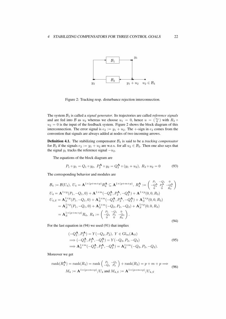
- B1 -r y1

?ru2 ∈ B3r��

y1 + u2B2�r

y2

Figure 2: Tracking resp. disturbance rejection interconnection.

The system B3 is called a signal generator. Its trajectories are called reference signalsand are fed into B as u2 whereas we choose u1 = 0, hence u = ( u2

0 ) with R3 ◦u2 = 0 is the input of the feedback system. Figure 2 shows the block diagram of thisinterconnection. The error signal is e2 := y1 + u2. The +-sign in e2 comes from theconvention that signals are always added at nodes of two incoming arrows.

Definition 4.1. The stabilizing compensator B2 is said to be a tracking compensatorfor B3 if the signals e2 := y1 + u2 are w.e.s. for all u2 ∈ B3. Then one also says thatthe signal y1 tracks the reference signal −u2.

The equations of the block diagram are

P1 ◦ y1 = Q1 ◦ y2, PA2 ◦ y2 = QA

2 ◦ (y1 + u2), R3 ◦ u2 = 0 (93)

The corresponding behavior and modules are

B4 := B(U4), U4 = A1×(p+m+p)RA4 ⊆ A1×(p+m+p), RA

4 :=

(P1 −Q1 0

−QA2 PA

2 −QA2

0 0 R3

)U4 = A1×p(P1,−Q1, 0) +A1×m(−QA

2 , PA2 ,−QA

2 ) +A1×p(0, 0, R3)

U4,S = A1×pS (P1,−Q1, 0) +A1×m

S (−QA2 , P

A2 ,−QA

2 ) +A1×pS (0, 0, R3)

= A1×pS (P1,−Q1, 0) +A1×m

S (−Q2, P2,−Q2) +A1×pS (0, 0, R3)

= A1×(p+m+p)S R4, R4 :=

(P1 −Q1 0−Q2 P2 −Q2

0 0 R3

).

(94)For the last equation in (94) we used (91) that implies

(−QA2 , P

A2 ) = Y (−Q2, P2), Y ∈ Glm(AS)

=⇒ (−QA2 , P

A2 ,−QA

2 ) = Y (−Q2, P2,−Q2)

=⇒ A1×mS (−QA

2 , PA2 ,−QA

2 ) = A1×mS (−Q2, P2,−Q2).

(95)

Moreover we get

rank(RA4 ) = rank(R4) = rank

(P1 −Q1

−Q2 P2

)+ rank(R3) = p+m+ p =⇒

M4 := A1×(p+m+p)/U4 and M4,S := A1×(p+m+p)/U4,S

(96)


are torsion modules and B4 is thus autonomous.The error behavior and its equation modules and system modules are

Berr := (idp, 0, idp) ◦ B4 = B(Uerr) ⊆ Wp,

Uerr := (◦(idp, 0, idp))−1 (U4) ⊆ A1×p, Merr := A1×p/Uerr ⊆ident.

M4,

Uerr,S := (◦(idp, 0, idp))−1 (U4,S) ⊆ A1×pS , Merr,S := A1×p

S /Uerr,S .

(97)

The second line in (97) follows from the exactness of the behavior functor A1×q/U 7→B(U). As a submodule of M4 the module Merr is torsion and therefore Berr is au-tonomous. By definition the behavior B2 is a tracking behavior for B3 if and only Berris stable or, equivalently, Merr,S = 0 or Uerr,S = A1×p

S .

Remark 4.2. For the computation of Uerr,S = (◦(idp, 0, idp))−1 (U4,S) we apply thefollowing standard algorithm: Assume a noetherian ring B and matrices and modules

R1 ∈ Bk1×`1 , P ∈ B`2×`1 ,

U1 := B1×k1R1 ⊆ B1×`1 , U2 := (◦P )−1 (U1) ⊆ B1×`2 .(98)

Let (X,R2) ∈ Bk2×(k1+`2) be a universal left annihilator of(R1

−P). This signifies that

B1×k2 ◦(X,R2)−→ B1×(k1+`2)◦(R1

−P)

−→ B1×`2 (99)

is exact or that X and R2 are universal matrices with XR1 = R2P . Then

U2 = B1×k2R2. (100)

For the computation ofUerr,S = (◦(idp, 0, idp))−1 (U4,S) let (X1, X2, X3, Rerr) ∈Akerr×(p+m+p+p)S be a universal left annihilator of

(R4

−(idp,0,idp)

)=

(P1 −Q1 0−Q2 P2 −Q2

0 0 R3

− idp 0 − idp

), hence

(X1, X2)(

P1 −Q1

−Q2 P2

)= (Rerr, 0), −X2Q2 +X3R3 −Rerr = 0.

(101)

By means of (54) the preceding equations are equivalent to

(X1, X2) = (Rerr, 0)(

P1 −Q1

−Q2 P2

)−1= (Rerr, 0)

(D2 N1

N2 D1

)= (RerrD2, RerrN1)

and Rerr(idp+N1Q2)−X3R3 = 0.(102)

Moreover(D2 N1

N2 D1

) ( P1 −Q1

−Q2 P2

)=(

idp o0 idm

)=⇒ idp = D2P1 −N1Q2 =⇒ D2P1 = idp+N1Q2 =

(54)idp+Hy1,u2

=⇒ (Rerr, X3)(D2P1

−R3

)= RerrD2P1 −X3R3 = 0.

(103)

Since (X1, · · · , Rerr) is a universal left annihilator of(

R4

(− idp,0,− idp)

)the matrix

(Rerr, X3) ∈ Akerr×(p+p)S is a universal left annihilator of

(D2P1

−R3

)∈ A

(p+p)×pS ;


this follows directly from (102). Since rank(R3) = p and thus also rank(D2P1

−R3

)= p

the kernel

A1×kerrS (Rerr, X3) = ker

(◦(D2P1

−R3

): A

1×(p+p)S → A1×p

S

)(104)

is free of dimension p = (p + p) − p and therefore we assume kerr = p w.l.o.g. Byconstruction the matrix Rerr generates Uerr,S , hence

Uerr,S = A1×pS Rerr, Merr,S = A1×p

S /A1×pS Rerr. (105)

Corollary 4.3. For the stabilizable behavior B1, its stabilizing compensator B2, thesignal generator B3, the interconnected behavior B from figure 2 and the derived datafrom above the component y1 of B1 tracks the reference signals −u2 ∈ B3 if and onlyif Rerr ∈ Glp(AS).

Theorem 4.4. Assume a stabilizable behavior B1 ⊂ Wp+m and a signal generatorB3 ⊂ Wp. Also consider the parametrization from Lemma 3.12 and the constructionof all stabilizing compensators B2 of B1 in Thm. 3.14 and the associated data.(i) There is a tracking stabilizing compensator for reference signals in B3 if and onlyif the following inhomogeneous linear equation has a solution (X,Y ) with entries inAS:

D02P1 = N1XP1 + Y R3, X ∈ Am×p

S , Y ∈ Ap×pS . (106)

(ii) If (106) is solvable then all tracking stabilizing compensators B(U2) are obtainedby the following steps:

1. Solve equation (106). Only the componentX is used for the further construction.

2. According to (53) define

(−Q2, P2) = (−Q02, P

02 ) +X(P1,−Q1),

(D2

N2

)=(D0

2

N02

)−(N1

D1

)X, hence

U1,S ⊕A1×mS (−Q2, P2) = A

1×(p+m)S ,

(P1 −Q1

−Q2 P2

)∈ Glp+m(AS).

(107)

3. Construct a stabilizing compensator B(U2) from (−Q2, P2) according to Thm.3.14.

The equations implyidp+Hy1,u2

= D2P1 = Y R3. (108)

Proof. 1. Necessity of (106): Assume that B2 is such a compensator so that the deriveddata from (93)- (105) are defined and Rerr ∈ Glp(AS). From (52) and (103) we get

D2 = D02 −N1X and RerrD2P1 = X3R3 with X,X3 ∈ A•×•S =⇒

D2P1 = R−1errX3R3 =⇒ D02P1 = N1XP1 + Y R3, Y := R−1errX3.

(109)

2. Sufficiency of (104): WithX from (106) we define the matrices from (107). Accord-ing to Lemma 3.12 and Thm. 3.14 the matrix (−Q2, P2) gives rise to several stabilizingcompensators B(U2) with U2,S = A1×m

S (−Q2, P2). The compensator B2 gives rise tothe data (97)-(105), in particular (Rerr, X3) is a universal left annihilator of

(D2P1

−R3

).

Equation (106) furnishes D2P1 = Y R3 and therefore (idp, Y ) ∈ Ap×(p+p)S is one

left annihilator of(D2P1

−R3

). This implies that there is a matrix Z ∈ Ap×p

S such thatZ(Rerr, X3) = (idp, Y ) and especially ZRerr = idp and Rerr ∈ Glp(AS). Accordingto Cor. 4.3 this signifies that B(U2) is a tracking compensator for B3. It is clear thatthis construction furnishes all tracking stabilizing compensators.


Example 4.5. We consider the data from Example 3.19, especially

P1 = (1 + a)s1, D02 = s−11 , N1 = −s−11 . (110)

Let B3 = B (AR3) , 0 6= R3 ∈ A, be an arbitrary autonomous signal generator. With(x, η) ∈ A1×2

S instead of (X,Y ) in equation (106) the latter gets the form

D02P1 = N1XP1 + Y R3 ⇐⇒ s−11 (1 + a)s1 = −s−11 x(1 + a)s1 + ηR3

⇐⇒ s−11 (1 + x)(1 + a)s1 = ηR3.(111)

The intersectionAS(1 + a)s1

⋂ASR3 = ASσ (112)

is a nonzero principal ideal. Hence there are nonzero ξ, η ∈ AS such that

σ = ξ(1 + a)s1 = ηR3 ⇐⇒ s−11 (1 + x)(1 + a)s1 = ηR3 with x := s1ξ − 1

⇐⇒ D02P1 = N1xP1 + ηR3.

(113)The stabilizing compensators from Example 3.19 constructed with this x or, more gen-erally, with x = s1ζξ − 1, ζ ∈ AS , track the reference signals from B3.

Disturbance rejection deals with the same stabilizable behavior B1, signal genera-tor B3 and interconnected behavior B4 as in the tracking case, but the control goal anderror behavior are different.

Definition and Corollary 4.6. The error behavior for disturbance rejection is Berr :=(idp, 0, 0)◦B4. The compensator B2 is said to reject disturbances from B3 if Berr is sta-ble. This signifies that inputs u1 = 0 and u2 ∈ B3 generate stable output componentsy1.

We state the corresponding theorem without its proof that is fully analogous to thetracking case.

Theorem 4.7. (Disturbance rejection) (i) The stabilizing compensator B(U2) of B(U1)rejects disturbances fromB3 if and only if the following inhomogeneous linear equation

N1Q02 = N1XP1 + Y R3, X ∈ Am×p

S , Y ∈ Ap×pS , (114)

has a solution (X,Y ) with entries in AS .(ii) If (114) is solvable all stabilizing compensators B2 of B1 for the rejection of signalsu2 ∈ B3 are obtained by the following construction steps:

1. Solve the equation (114) where only X is needed for the further construction.

2. Define (−Q2, P2) := (−Q02, P

02 ) + X(P1,−Q1) according to (53). Use Thm.

3.14 to construct the matrix

(−QA2 , P

A2 ) ∈ Am×(p+m) and U2 := A1×m(−QA

2 , PA2 ) ⊆ A1×(p+m)

such that U2,S = A1×mS (−Q2, P2) and U1,S ⊕ U2,S = A

1×(p+m)S .

(115)

The behaviors B(U2) are the desired compensators that are essentially parametrizedby the components X ∈ Am×p of the solutions of (114). The equations imply

Hy1,u2=

(54)N1Q2 = Y R3. (116)


4.2 Model matchingWe consider a stabilizable behavior B1 = B(U1) ⊆ Wp+m and its parametrized familyof stabilizing compensators B(U2) with U1,S ⊕ U2,S = A

1×(p+m)S as described in

Sections 3.3 and 3.4. In addition we consider a model input/output behavior

B(Um), Um = A1×p(Pm,−Qm), (Pm,−Qm) ∈ Ap×(p+p), Hm = P−1m Qm,(117)

with transfer matrix Hm. The IO property signifies that Pm ∈ Glp(Q). The intercon-nection of these behaviors is realized by taking u2 ∈ W (τ)p as input both for B2 andfor Bm where we choose u1 = 0 as in the tracking case. This interconnection is thusdescribed by the trajectories (y1, y2, u2, ym)> and the equations

P1 ◦ y1 = Q1 ◦ y2, PA2 ◦ y2 = QA

2 ◦ (u2 + y1), Pm ◦ ym = Qm ◦ u2 (118)

that give rise to the behavior

B4 = B(U4), U4 = A1×(p+m+p+p)R4, RA4 :=

(P1 −Q1 0 0

−QA2 PA

2 −QA2 0

0 0 −Qm Pm

), hence

U4,S = A1×(p+m+p+p)R4, R4 :=

(P1 −Q1 0 0−Q2 P2 −Q2 00 0 −Qm Pm

)with

rank(R4) = p+m+ p since(

P1 −Q1

−Q2 P2

)∈ Glp+m(Q) and Pm ∈ Glp(Q).

(119)The error signal is defined as e = y1 − ym and the error behavior as Berr =

(idp, 0, 0,− idp) ◦ B4.

Definition 4.8. The stabilizing compensator is called model matching for Bm if Berr isautonomous and stable. One also says that y1 matches the model ym for all inputs u2.

The equation module of Berr is Uerr = ((idp, 0, 0,− idp)−1

(U4) ⊆ A1×p and B2is model matching if and only Uerr,S = A1×p

S where

Uerr,S = ((idp, 0, 0,− idp))−1

(U4,S) = A1×kerrS Rerr. (120)

Analogous computations to those for Cor. 4.3 furnish

Uerr,S = A1×kerrRerr, Rerr = −X3Pm where

A1×kerrX3 = ker(◦(PmN1Q2 −Qm) : A1×p

S → A1×pS

).

(121)

Corollary 4.9. The stabilizing compensator B2 is model-matching for the IO behaviorBm, i.e., Uerr,S = A1×p

S , if and only if Bm is stable and Hm = N1Q2 =(54)

Hy1,u2.

Proof. =⇒: The equations A1×kerrRerr = A1×pS andRerr = −X3Pm imply A1×pPm =

A1×pS and hence Pm ∈ Glp(AS) and rank(X3) = p. According to Lemma and Def.

3.6 Bm is stable and X3 can be cancelled as left factor. But

X3(PmN1Q2 −Qm) = 0 =⇒ Pm(N1Q2 −Hm) = 0 =⇒ Hm = N1Q2.

⇐=: If

Hm = N1Q2 =⇒ Pm(N1Q2 −Hm) = PmN1Q2 −Qm = 0 =⇒kerr = p, X3 = idp =⇒ Rerr = −Pm =⇒

Pm∈Glp(AS)Rerr ∈ Glp(AS).

5 ALGORITHMS 27

Theorem 4.10. Assume a stabilizable behaviorB1 = B(U1) whereU1 = A1×p(P1,−Q1)and (P1,−Q1) ∈ Ap×(p+m) such that the exact sequences (49) and (50) exist. Alsoassume a stable model IO behavior Bm = B(Um) where Um = A1×p(Pm,−Qm),(Pm,−Qm) ∈ Ap×(p+p) and Pm ∈ Glp(AS).(i) Then B1 admits a model-matching stabilizing compensator for Bm if and only theinhomogeneous linear equation

N1Q02 −Hm = N1XP1, X ∈ Am×p

S , (122)

has a solution X with entries in AS .(ii) If (122) is solvable then all stabilizing compensators for matching the model Bmare obtained with the following steps:

1. Solve (122) and use X to define (−Q2, P2) = (−Q02, P

02 ) + X(P1,−Q1) ac-

cording to (53).

2. Use Thm. 3.14 to construct a module U2 = A1×m(−QA2 , P

A2 ) with U2,S =

A1×mS (−Q2, P2).

Then B(U2) is the desired compensator.

Proof. (i)1. Necessity of (122): From Cor. 4.9 we getHm = N1Q2. From (−Q2, P2) =(−Q0

2, P02 ) +X(P1,−Q1) we infer Q2 = Q0

2 −XP1 and hence (122).2. Sufficiency of (122): Perform the steps above. The equations (122) and Q2 =Q0

2 −XP1 imply N1Q2 = Hm. By Cor. 4.9 the latter equation signifies that B(U2) ismodel matching.(ii) is a simple consequence of (i).

5 AlgorithmsAlmost all steps of the preceding constructions can be carried out algorithmically. Wedescribe the algorithms, but leave to experts in Computer Algebra [10], [20] to imple-ment them. We do not discuss addition and multiplication in K ⊂ A ⊂ Q. Since Kcontains arbitrary Laurent series it is clear that in practical examples one has to con-sider rational coefficient functions with coefficients in Q(i) or standard functions likezk exp(z−1), k ∈ Z. Euclidean division in A is possible. Also the theory of f.g.A-modules is constructive. In particular, the freeness (=projectivity) and the torsionproperty of a f.g. A-left module can be decided. The main theorem 2.7 of [6] describesa test for weak exponential stability of most differential operators and therefore a testfor the inclusion s ∈ S. If q = ba−1, 0 6= a, b ∈ A, is a nonzero element of Q then

As := {f ∈ A; fq ∈ A} = (◦b)−1(Aa) and (q ∈ AS ⇐⇒ s ∈ S) (123)

can be computed, hence q ∈ AS can be decided. A f.g. torsion module M is con-structively isomorphic to A/AF where 0 6= F ∈ A. Since f.g. stable modules areclosed under isomorphisms the module M is stable if and only A/AF is stable andthis is equivalent to F ∈ S that can be decided (in most cases). The construction ofcompensators in Thms. 4.4, 4.7 and 4.10 depends on the solution of inhomogeneouslinear equations

AXB = C, A,B,C,X ∈ A•×•S , (124)

6 CONCLUSION 28

where A,B,C are given and a solution X is sought. These equations can always besolved. By multiplying A from the left and B from the right by common denominatorsin S we may and do assume wlog thatA andB, but not necessarilyC have entries in A.Every matrix A with entries in A is equivalent to a diagonal matrix. One can constructinvertible matrices U1 and U2 and a square diagonal matrix D = diag(a1, · · · , ar)with r = rank(A) and nonzero ai such that

U1AU2 = A :=(D(a) 00 0

), U1, U2 ∈ Gl•(A), D(a) = diag(a1, · · · , ar), 0 6= ai ∈ A.

(125)One can even choose a1 = · · · = ar−1 = 1. Consider the analogous decompositionfor B, i.e.,

V1BV2 = B :=(D(b) 00 0

), U1, U2 ∈ Gl•(A), D = diag(b1, · · · , bs), 0 6= bj ∈ A.

(126)Then

AXB = C ⇐⇒ AXB = C ⇐⇒(D(a) 00 0

)X(D(b) 00 0

)= C

where X := U−12 XV −11 , C := U1CV2.(127)

The last equation implies

Cij =

{aiXijbj if i ≤ r, j ≤ s0 otherwise

and ∀i ≤ r∀j ≤ s : Xij = a−1i Cijb−1j . (128)

Lemma 5.1. (i) The linear system AXB = C is solvable in A•×•S if and only if{∀i > r : Ci− = 0 and ∀j > s : C−j = 0

∀i ≤ r∀j ≤ s : a−1i Cijb−1j ∈ AS

. (129)

(ii) If the system is solvable then

L ={X; AXB = C

}={X ∈ A•×•S ; ∀i ≤ r∀j ≤ s; Xij = a−1i Cijb

−1j

}L := {X; AXB = C} = U2LV1 =

{U2XV1; X ∈ L

}.

(130)

(iii) For the homogeneous systems this implies

L0 :={X; AXB = 0

}={X ∈ A•×•S ; ∀i ≤ r∀j ≤ s : Xij = 0

},

L0 := {X; AXB = 0} = U2L0V1, hence also L = X1 + L0, X1 ∈ L.

(131)

The conditions in (129) can be checked and therefore the linear systemsAXB = Cwith matrices with entries in AS can be solved.

6 ConclusionIn this paper we present a new constructive theory of stabilization and control for LTVdifferential systems whose computer implementation is left to younger colleagues. Ex-amples 3.19 and 4.5 computed by hand illustrate the theory. The paper extends the LTItheories from, for instance, [8], [9, §9.6, pp. 488-506], [22, §5.7, pp. 151-155], to the

REFERENCES 29

LTV situation. Most papers (google search) on this subject in the literature deal withKalman’s state space systems (cf. [21, pp. 280-284]) of the form

x′(t) = A(t)x(t) +B(t)u(t), y(t) = C(t)x(t) +D(t)u(t), (132)

whereas we consider general implicit linear differential systems of arbitrary order.Arbitrary analytic or even smooth coefficient functions are unsuitable for such systems.It has turned out that smooth functions derived from the field of locally convergentPuiseux-series have all necessary properties. These coefficient functions approximatelarge classes of continuous functions and this enables the application of the presenttheory to even more general systems. The important problem of robustness in thiscontext has, however, not yet been solved. We also employ a new kind of behaviorsand their weak exponential stability that were introduced in the recent paper [7]. Theresults of the latter paper are essential for the proofs of the present one. In Remark3.20 we explain differences and similarities to [5, Ch. 11, pp. 545-554] that, to ourknowledge, is the only work where tracking and disturbance rejection of LTV systemshave been discussed in the same generality.Acknowledgement: I thank the two reviewers for their efforts and suggestions.

References[1] B.D.O. Anderson, A. Ilchmann, F.R. Wirth, ’Stabilizability of linear time-varying

systems’; Systems and Control Letters 62(2013), 747-755

[2] T. Berger, A. Ilchmann, F.R. Wirth, ’Zero dynamics and stabilization for analyticlinear systems’, Acta Appl. Math. 138(2014), 17-57

[3] I. Blumthaler, ’Stabilisation and control design by partial output feedback and bypartial interconnection’, International Journal of Control, 85(2012), 1717-1736

[4] I. Blumthaler, U. Oberst, ’Design, parametrization, and pole placement of sta-bilizing output feedback compensators via injective cogenerator quotient signalmodules’, Linear Algebra and its Applications 436(2012), 963-1000

[5] H. Bourlès, B. Marinescu, Linear Time-Varying Systems, Springer, Berlin, 2011

[6] H. Bourlès, B. Marinescu, U. Oberst, ’Exponentially stable linear time-varyingdiscrete behaviors’, SIAM J. Control Optim., 53(2015), 2725-2761

[7] H. Bourlès, B. Marinescu, U. Oberst, ’Weak exponential stability of linear time-varying differential behaviors’, Linear Algebra and its Applications 486(2015),523-571

[8] F.M. Callier, C.A. Desoer, Multivariable Feedback Systems, Springer, New York,1982

[9] C.-T. Chen, Linear System Theory and Design, Harcourt Brace, FortWorth, 1984

[10] F. Chyzak, A. Quadrat, D. Robertz, ’OreModules: A symbolic package for thestudy of multidimensional linear systems’ in J. Chiasson, J.-J. Loiseau (Eds.),Applications of Time-Delay Systems, Lecture Notes in Control and InformationSciences 352, pp. 233-264, Springer, Berlin, 2007

REFERENCES 30

[11] P.M. Cohn, Free Ideal Rings and Localization in General Rings, Cambridge Uni-versity Press, Cambridge, 2006

[12] M. Fliess, ’Some basic structural properties of generalized linear systems’, Sys-tems and Control Letters 15(1990), 391-396

[13] J.C. McConnell, J.C. Robson, Noncommutative Noetherian Rings, John Wileyand Sons, Chichester, 1987

[14] Vu N. Phat, V. Jeyakumar, ’Stability, stabilization and duality for linear time-varying systems’, Optimization 59(2010), 447-460

[15] M. van der Put, M. F. Singer, Galois Theory of Linear Differential Equations,Springer, Berlin, 2003

[16] A. Quadrat, ’On a generalization of the Youla-Kucera parametrization. Part II:The lattice approach to MIMO systems’, Mathematics of Control, Signals andSystems 18(2006), 199-235

[17] A. Quadrat, ’Systèmes et Structures: Une approche de la théorie des systèmes parl’analyse algébrique constructive’, Thèse d‘habilitation à diriger des recherches,Université de Nice Sofia-Antipolis, 2010

[18] A. Quadrat, Algebraic Analysis of Linear Functional Systems, book in prepara-tion, 2015

[19] R. Ravi, A.M. Pascoal, P.P. Khargonekar, ’Normalized coprime factorizations forlinear time-varying systems’, Systems and Control Letters 18(1992), 455-465

[20] D. Robertz, ’Recent Progress in an Algebraic Analysis Approach to Linear Sys-tems’, Mult Syst Sign Process 26(2015), 349-380

[21] W.J. Rugh, Linear System Theory, Prentice Hall, Upper Saddle River, NJ, 1996

[22] M. Vidyasagar, Control System Synthesis: A Factorization Approach, The MITPress, Cambridge, Ma., 1985

Documents

Stabilizing compensators for linear time-varying differential systems