Stable border bases for ideals of points

Journal of Symbolic Computation 43 (2008) 883–894

Contents lists available at ScienceDirect

Journal of Symbolic Computation

journal homepage: www.elsevier.com/locate/jsc

Stable border bases for ideals of pointsJohn Abbott a, Claudia Fassino a,1, Maria-Laura Torrente ba Dip. di Matematica, Università di Genova, Via Dodecaneso 35, 16146 Genova, Italyb Scuola Normale Superiore, Piazza dei Cavalieri 7, 56126 Pisa, Italy

a r t i c l e i n f o

Article history:Received 11 October 2007Accepted 15 May 2008Available online 3 June 2008

Keywords:Empirical pointsVanishing idealBorder bases

a b s t r a c t

Let X be a set of points whose coordinates are known with limitedaccuracy; our aim is to give a characterization of the vanishing idealI(X) independent of the data uncertainty. We present a methodto compute, starting from X, a polynomial basis B of I(X) whichexhibits structural stability, that is, if X is any set of points differingonly slightly from X, there exists a polynomial set B structurallysimilar toB, which is a basis of the perturbed ideal I(X).

© 2008 Elsevier Ltd. All rights reserved.

1. Introduction

In this paper we present a method for computing ‘‘structurally stable’’ border bases of ideals ofpoints whose coordinates are affected by errors.If X is a set of ‘‘empirical’’ points, representing real-world measurements, then typically the

coordinates are known only imprecisely. Roughly speaking, if X is another set of points, each differingby less than the uncertainty from the corresponding element ofX, then the two sets can be consideredas equivalent. Nevertheless, it can happen that their vanishing ideals have very different bases —this is a well known phenomenon in Gröbner basis theory. In order to emphasize the ‘‘numericalequivalence’’ of X and its perturbation X, we look for a common characterization of the vanishingideals I(X) and I(X). More precisely our goal is to determine a polynomial basis B of the vanishingideal I(X)which exhibits structural stability: namely, there is a basis B for the perturbed ideal I(X),sharing the same structure as B, and whose coefficients differ only slightly, provided that X differsfrom X by only a small amount (up to some limit).The decision to use border bases to describe vanishing ideals of sets of empirical points was due to

two main reasons: border bases have always been considered a numerically stable tool (see Kehreinet al. (2005), Kreuzer and Robbiano (2005), Mourrain and Trébuchet (2005), Mourrain (2007) and

E-mail addresses: [email protected] (J. Abbott), [email protected] (C. Fassino), [email protected] (M.-L. Torrente).1 Tel.: +39 0103536822; fax: +39 0103536752.

0747-7171/$ – see front matter© 2008 Elsevier Ltd. All rights reserved.doi:10.1016/j.jsc.2008.05.002

http://www.elsevier.com/locate/jsc

http://www.elsevier.com/locate/jsc

mailto:[email protected]



http://dx.doi.org/10.1016/j.jsc.2008.05.002

884 J. Abbott et al. / Journal of Symbolic Computation 43 (2008) 883–894

Stetter (2004)); furthermore, it is easy to study their structure, i.e. the support of their polynomials, asit is completely determined once a suitable order idealO has been chosen. An alternative approach ispresented in Sauer (2007) who extends the notion of H-basis to an ‘‘approximate ideal" of empiricalpoints.We introduce the notion of stable quotient basis: given a setX of empirical points and a permitted

tolerance ε, a stable quotient basisO guarantees the existence of anO-border basis B for the vanishingideal I(X)where X is any set of points perturbed by amounts less than the tolerance ε. Once a stablequotient basis O has been found, the corresponding stable border basis can be obtained by somesimple combinatorical and linear algebra computations; so we focus our attention on determiningO.An alternative approach to the problem, presented in Heldt et al. (2006), is to use singular value

decomposition of matrices to obtain a set of polynomials which are not required to vanish on X butmust nevertheless assume particularly small values there. In contrast, a stable border basis alwayscomprises polynomials which vanish on X.This paper is organized as follows. In Section 2 we introduce the concepts and tools we shall

use. Section 3 provides a formal description of our problem. The main result, the SOI algorithmfor computing a stable order ideal, is presented in Section 4. In Section 5 we give some numericalexamples illustrating the functioning of the algorithm. Finally, Section 6 is anAppendixwhich containsthe proof of a basic result about the first order approximation of rational functions, useful for the erroranalysis of the sensitivity of the border basis computation.

2. Basic definitions and notation

This section contains basic definitions and notation used later in the paper. To simplify thepresentation, we shall implicitly suppose that each finite set of points or polynomials is in fact a tuple,so that the elements are ordered in some way, and we can refer to the k-th element using the index k.Let n ≥ 1; we recall (see Kreuzer and Robbiano (2000, 2005)) some basic concepts related to the

polynomial ring P = R[x1, . . . , xn].

Definition 1. Let X = {p1, . . . , ps} be a non-empty finite set of points of Rn and let G = {g1, . . . , gk}be a non-empty finite set of polynomials.

(a) The ideal I(X) = {f ∈ P | f (pi) = 0 ∀pi ∈ X} is called the vanishing ideal of X.(b) The R-linear map evalX : P → Rs defined by evalX(f ) = (f (p1), . . . , f (ps)) is called the

evaluation map associated to X. For brevity, we write f (X) to mean evalX(f ).(c) The evaluation matrix of G associated to X, written as MG(X) ∈ Mats×k(R), is defined as havingentry (i, j) equal to gj(pi), i.e. whose columns are the images of the polynomials gj under theevaluation map.

Definition 2. Let Tn be the monoid of power products of P and let O be a non-empty subset of Tn.

(a) The factor closure (abbr. closure) ofO is the setO of all power products in Tn which divide somepower product of O.

(b) The set O is called an order ideal if O = O, i.e. if O is factor closed.(c) Let I ⊆ P be a zero-dimensional ideal, and s = dim(P/I); if O is factor closed and the residueclasses of its elements form a basis of P/I then we call it a quotient basis for I .

(d) Let O be factor closed; the border ∂O of O is defined by

∂O = (x1O ∪ · · · ∪ xnO) \ O.

(e) If O is factor closed then the elements of the minimal set of generators of the monomial idealcorresponding to Tn\O are called the corners of O.

Definition 3. LetO = {t1, . . . , tµ} be an order ideal, and let ∂O = {b1, . . . , bν} be the border ofO. LetB = {g1, . . . , gν} be a set of polynomials having the form gj = bj −

∑µ

i=1 αijti where each αij ∈ R.Let I ⊆ P be an ideal containingB. If the residue classes of the elements ofO form an R-vector spacebasis of P/I thenB is called a border basis of I founded onO, or more brieflyB is anO-border basisof I .

J. Abbott et al. / Journal of Symbolic Computation 43 (2008) 883–894 885

Proposition 4 (Existence and Uniqueness of Border Bases). Let I ⊆ P be a zero-dimensional ideal, andlet O = {t1, . . . , tµ} be a quotient basis for I. Then there exists a unique O-border basisB of I.

Proof. See Proposition 6.4.17 in Kreuzer and Robbiano (2005). �

Later on, in order to measure the distances between points of Rn, we will use the euclidean norm‖ · ‖. Additionally, given an n× n positive diagonal matrix E, we shall also use the weighted 2-norm‖ · ‖E as defined in Dahlquist et al. (1974). For completeness, we recall here their definitions:

‖v‖ :=

√√√√ n∑j=1

v2j and ‖v‖E := ‖Ev‖.

We recall the definition of empirical point (see Stetter (2004) and Abbott et al. (2007)).

Definition 5. Let p ∈ Rn be a point and let ε = (ε1, . . . , εn), with each εi ∈ R+, be the vector ofthe componentwise tolerances. An empirical point pε is the pair (p, ε), where we call p the specifiedvalue and ε the tolerance.

Let pε be an empirical point. We define its ellipsoid of perturbations:

N(pε) = {p ∈ Rn : ‖p− p‖E ≤ 1}

where the positive diagonal matrix E = diag(1/ε1, . . . , 1/εn). This set contains all the admissibleperturbations of the specified value p, i.e. all points differing from p by less than the tolerance.Henceforth we shall assume that all the empirical points share the same tolerance ε, as is

reasonable if they derive from real-world data measured with the same accuracy. In particular thisassumption allows us to use the E-weighted norm on Rn to measure the distance between empiricalpoints.Given a finite set Xε of empirical points all sharing the same tolerance ε, we introduce the concept

of a slightly perturbed set of points X by means of the following definition.

Definition 6. Let Xε = {pε1, . . . , pεs } be a set of empirical points with uniform tolerance ε and with

X ⊂ Rn. Each set of points X = {p1, . . . , ps} ⊂ Rn whose elements satisfy

(p1, . . . , ps) ∈s∏i=1

N(pεi )

is called an admissible perturbation of Xε .

Finally we introduce the definition of distinct empirical points.

Definition 7. The empirical points pε1 and pε2, with specified values p1, p2 ∈ Rn, are said to be distinct

if

N(pε1) ∩ N(pε2) = ∅.

3. The formal problem

We shall use the concept of empirical point to describe formally the given uncertain data: the inputX is viewed as the set of specified values ofXε , which consists of s distinct empirical points all sharingthe same fixed tolerance ε.Given the set Xε , we want to determine a structurally stable basis B of the vanishing ideal I(X).

Intuitively, a basis B of I(X) is considered to be structurally stable if, for each admissibleperturbation X of Xε , it is possible to produce a basis B of I(X) by means of a slight and continuousvariation of the coefficients of the polynomials of B, that is there exists a basis B of I(X) whosepolynomials have the same support as the corresponding polynomials of B. Given a polynomialbasisB, we will call the union of the supports of its polynomials the structure ofB.A good starting point for us is the concept of border basis (see Kreuzer and Robbiano (2005) and

Stetter (2004)). In fact the structure of a border basis is easily computable and completely determined


by the quotient basisO uponwhich the border basis is founded (see Definition 3). Using border bases,the problemof computing a structurally stable representation of the vanishing idealI(X) thus reducesto the problem of finding a quotient basis O for I(X) valid for every admissible perturbation X. Thefollowing definition captures this notion and generalizes it to any order ideal.

Definition 8. Let O be an order ideal, then O is stable w.r.t. Xε if the evaluation matrix MO(X) hasfull rank for each admissible perturbation X of Xε .

The following proposition highlights the importance of stable quotient bases (see also Proposition4.20 in Mourrain and Ruatta (2002)).

Proposition 9. Let Xε be a set of s distinct empirical points, and let O = {t1, . . . , ts} be a quotientbasis for I(X) which is stable w.r.t. Xε . Then, for each admissible perturbation X of Xε , the vanishingideal I(X) has an O-border basis. Furthermore, if ∂O = {b1, . . . , bν} is the border of O then B consistsof ν polynomials of the form

gj = bj −s∑i=1

αijti for j = 1 . . . ν (1)

where the coefficients aij ∈ R satisfy the linear systems

bj(X) =s∑i=1

αijti(X).

Proof. Let X be an admissible perturbation of Xε and let evalX : P → Rs be the evaluation mapassociated to the set X. It is easy to prove that I(X) = ker(evalX) and consequently, that the quotientring P/I(X) is isomorphic toRs as a vector space. SinceO is stablew.r.t. the empirical setXε , it followsthat {t1(X), . . . , ts(X)} are linearly independent vectors. Moreover #X = #O, so the residue classesof the elements of O form a vector space basis of P/I(X).Let vj = bj(X) be the evaluation vector associated to the power product bj lying in the border ∂O;

each vj can be expressed as

vj =

s∑i=1

αijti(X) for some αij ∈ R.

For each j we define the polynomial gj = bj −∑si=1 αijti; by construction evalX(gj) = 0, and so

B = {g1, . . . , gν} is contained in I(X); it follows that B is the O-border basis of the ideal I(X). �

We observe that the coefficients αij of each polynomial gj ∈ B are just the components of thesolution αj of the linear system MO(X) αj = bj(X). It follows that αij are continuous functions of thepoints of the set X and so, since O is stable w.r.t. Xε , they undergo only continuous variations as Xchanges. Now, the definition of stable border basis follows naturally.

Definition 10. Let Xε be a finite set of distinct empirical points, let O be a quotient basis for thevanishing ideal I(X). If O is stable w.r.t. Xε then the O-border basis B for I(X) is said to be stablew.r.t. the set Xε .

The problemof computing a stable border basis of the vanishing ideal of a setXε of empirical pointsis therefore completely solved once we have found a quotient basis O which is stable w.r.t. Xε . If wehave such anO, Proposition 9 and the subsequent observation on the continuity of the coefficients αijprove the existence of the corresponding stable border basis of the ideal I(X). The problem of theeffective computation of a stable quotient basis is addressed in Section 4.We end this section by observing that any O-border basis of the vanishing ideal I(X) is stable

w.r.t. Xδ for a sufficiently small value of the tolerance δ. This is equivalent to saying that any quotientbasis O of I(X) has a ‘‘region of stability’’, as the following proposition shows.

Proposition 11. Let X be a finite set of points of Rn and I(X) be its vanishing ideal; let O be a quotientbasis for I(X). Then there exists a tolerance δ = (δ1, . . . , δn), with δi > 0, such that O is stable w.r.t. Xδ .


Proof. Let MO(X) be the evaluation matrix of O associated to the set X; then MO(X) is a structuredmatrix whose coefficients depend continuously on the points in X. Since, by hypothesis, theO-border basis of the vanishing ideal I(X) exists, it follows thatMO(X) is invertible. Recalling that thedeterminant is a polynomial function in the matrix entries, and noting that the entries of MO(X) arepolynomials in the points’ coordinates, we can conclude that there exists a tolerance δ = (δ1, . . . , δn),with each δi > 0, such that det(MO(X)) 6= 0 for any perturbation X of X. �

Nevertheless, since the tolerance ε of the empirical points in Xε is given a priori by themeasurements, Proposition 11 does not solve our problem. If the given tolerance ε is larger than the‘‘region of stability’’ of a chosen quotient basis O, the corresponding border basis will not be stablew.r.t. Xε; such a situation is shown in the following example.

Example 12. Let Xε be the set of empirical points having

X = {(−1,−5), (0,−2), (1, 1), (2, 4.1)} ⊂ R2

as the set of specified values and ε = (0.15, 0.15) as the tolerance; let

X = {(−1+ e1,−5+ e2), (e3,−2+ e4), (1+ e5, 1+ e6), (2+ e7, 4.1+ e8)}

be a generic admissible perturbation of Xε , where the parameters ei ∈ R satisfy

‖(e1, e2)‖E ≤ 1 ‖(e3, e4)‖E ≤ 1 ‖(e5, e6)‖E ≤ 1 ‖(e7, e8)‖E ≤ 1.

Consider first O1 = {1, x, y, y2}, which is a quotient basis for I(X). The correspondingborder basis B1 of I(X) is not stable w.r.t. Xε . Indeed, consider the perturbation X =

{(−1,−5), (0,−2), (1, 1), (2, 4)} ofXε . The evaluationmatrixMO1(X) is singular, so noO1-borderbasis of I(X) exists. It follows that O1 is not stable w.r.t. Xε since its ‘‘region of stability’’ is too smallw.r.t. the given tolerance ε.Now consider the quotient basis O2 = {1, y, y2, y3}, which is stable w.r.t. Xε . In fact, for each

perturbation X of Xε , we see that MO2(X) is a Vandermonde matrix whose determinant is equal to(e4−e2+3)(e6−e2+6)(e8−e2+9.1)(e6−e4+3)(e8−e4+6.1)(e8−e6+3.1). Since each |ei| ≤ 0.15,it follows that, for each perturbation X, the matrixMO2(X) is invertible, and so it is always possible tocompute an O2-border basis of the ideal I(X). In fact O2 is stable w.r.t. X(δ1,δ2), where δ1 is unlimitedand δ2 = 1.5. �

4. A practical solution

In this section we address the problem of finding an order idealO stable w.r.t. a given finite set of sdistinct empirical points,Xε . IfO contains s power products, that is ifO is a quotient basis of I(X), thecorresponding stable border basis is also computed. The numerical examples show that O can havecardinality less than swhen the tolerance on the points is, in some sense, too large; this phenomenonis illustrated in Example 20.We plan to investigate further the causes of this ‘‘premature termination’’.Since in real-world measurements the tolerance ε present in the data is relatively small, our

interest is focused on small perturbations X of the empirical set Xε . For this reason our approachis based on a first order error analysis of the problem. We present in Section 4.3 an algorithm whichcomputes a stable order ideal O. In order to investigate the stability of O we use some results onthe first order approximation of rational functions (see Section 4.1) and we introduce a parametricdescription of the admissible perturbations X of Xε (see Section 4.2).If the output of the algorithm is actually a quotient basis then the corresponding stable border

basis B exists for I(X). To determine B it suffices to find the border of O (a simple combinatoricalcomputation), and then for each element of the border solve a linear system (see Proposition 9).

4.1. Remarks on first order approximation

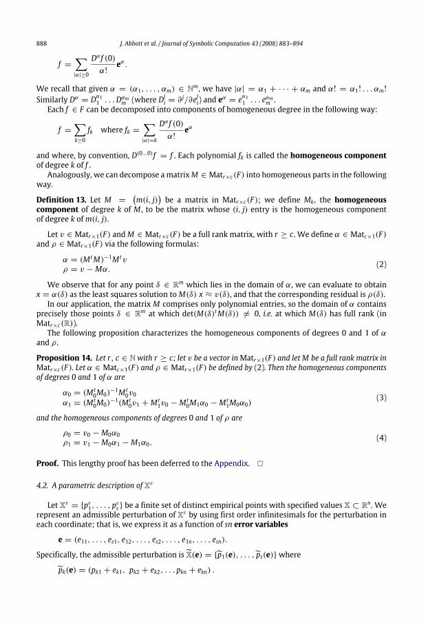
Let e = (e1, . . . , em) be indeterminates and F = R(e) be the field of rational functions. We usemulti-index notation to give the formal Taylor expansion of f ∈ F at 0:


f =∑|α|≥0

Dα f (0)α!

eα.

We recall that given α = (α1, . . . , αm) ∈ Nm, we have |α| = α1 + · · · + αm and α! = α1! . . . αm!

Similarly Dα = Dα11 . . .Dαmm (where D

ji = ∂

j/∂eji) and eα= eα11 . . . e

αmm .

Each f ∈ F can be decomposed into components of homogeneous degree in the following way:

f =∑k≥0

fk where fk =∑|α|=k

Dα f (0)α!

eα

and where, by convention, D(0...0)f = f . Each polynomial fk is called the homogeneous componentof degree k of f .Analogously, we can decompose amatrixM ∈ Matr×c(F) into homogeneous parts in the following

way.

Definition 13. Let M =(m(i, j)

)be a matrix in Matr×c(F); we define Mk, the homogeneous

component of degree k of M , to be the matrix whose (i, j) entry is the homogeneous componentof degree k ofm(i, j).

Let v ∈ Matr×1(F) andM ∈ Matr×c(F) be a full rank matrix, with r ≥ c . We define α ∈ Matc×1(F)and ρ ∈ Matr×1(F) via the following formulas:

α = (M tM)−1M tvρ = v −Mα. (2)

We observe that for any point δ ∈ Rm which lies in the domain of α, we can evaluate to obtainx = α(δ) as the least squares solution toM(δ) x ≈ v(δ), and that the corresponding residual is ρ(δ).In our application, the matrix M comprises only polynomial entries, so the domain of α contains

precisely those points δ ∈ Rm at which det(M(δ)tM(δ)) 6= 0, i.e. at which M(δ) has full rank (inMatr×c(R)).The following proposition characterizes the homogeneous components of degrees 0 and 1 of α

and ρ.

Proposition 14. Let r, c ∈ Nwith r ≥ c; let v be a vector inMatr×1(F) and let M be a full rank matrix inMatr×c(F). Let α ∈ Matc×1(F) and ρ ∈ Matr×1(F) be defined by (2). Then the homogeneous componentsof degrees 0 and 1 of α are

α0 = (M t0M0)−1M t0v0

α1 = (M t0M0)−1(M t0v1 +M

t1v0 −M

t0M1α0 −M

t1M0α0)

(3)

and the homogeneous components of degrees 0 and 1 of ρ are

ρ0 = v0 −M0α0ρ1 = v1 −M0α1 −M1α0.

(4)

Proof. This lengthy proof has been deferred to the Appendix. �

4.2. A parametric description of Xε

Let Xε = {pε1, . . . , pεs } be a finite set of distinct empirical points with specified values X ⊂ Rn. We

represent an admissible perturbation of Xε by using first order infinitesimals for the perturbation ineach coordinate; that is, we express it as a function of sn error variables

e = (e11, . . . , es1, e12, . . . , es2, . . . , e1n, . . . , esn).

Specifically, the admissible perturbation is X(e) = {p1(e), . . . , ps(e)}where

pk(e) = (pk1 + ek1, pk2 + ek2, . . . pkn + ekn) .


The conditions on the values of the ekj such that each pk is an admissible perturbation of the point pkare equivalent to the following:

‖(ek1, . . . , ekn)‖E ≤ 1 for each k. (5)

We observe that the coordinates of each perturbed point pk(e) are elements of the polynomialring R = R[e] and that each variable ekj represents the perturbation in the j-th coordinate of thespecified value pk. The domain of the perturbed set X(e), viewed as a function of sn variables, isdenoted by Dε . Obviously, if δ ∈ Dε we have

‖δ‖2 =

n∑j=1

s∑k=1

δ2kj ≤

n∑j=1

sε2j ,

and consequently

‖δ‖ ≤√s‖ε‖. (6)

To keep evident the dependence on the error variables e, we extend the concepts of Definition 1,namely the evaluation map of a polynomial f ∈ P and the evaluation matrix of a set of polynomialsG = {g1, . . . , gk} ⊂ P , to a generic perturbed set X(e), using the following notation:

evalX(e)(f ) = (f (p1(e)), . . . , f (ps(e))) ∈ Rs

for brevity denoted by f (X(e)); similarly we write the evaluation matrix

MG(X(e)) =(g1(X(e)), . . . , gk(X(e))

)∈ Mats×k(R).

4.3. The SOI algorithm

In this section we present the SOI algorithm which computes an order ideal O stable w.r.t theempirical set Xε .The strategy for computing a stable order ideal O is the following. As in the Buchberger–Möller

algorithm (see Buchberger and Möller (1982) and Abbott et al. (2000)) the set O is built stepwise:initially O comprises just the power product 1; then at each iteration, a new power product t isconsidered. If the evaluation matrix MO∪{t}(X(δ)) has full rank for all δ ∈ Dε then t is added to O;otherwise t is added to the corner set of the order ideal.A first observation concerns the choice of the power product t to analyze at each iteration: any

strategy that chooses a term t such that the set O ∪ {t} is factor closed can be applied. A possibletechnique is the one used in the Buchberger–Möller algorithm, where the chosen power product tis the smallest candidate according to a fixed term ordering σ . The version of the SOI Algorithmpresented below employs this latter strategy. Note that σ is used only as a computational tool forchoosing t; in fact the final computed setO is not, in general, the same as thatwhichwould be obtainedby processing the set X using the Buchberger–Möller algorithm with the same term ordering (seeExamples 16 and 17).Another observation concerns the main check of the algorithm: note that the rank condition is

equivalent to checking whether ρ(δ), the component of the evaluation vector t(X(δ)) orthogonal tothe column space of the matrix MO(X(δ)), vanishes for some δ ∈ Dε . This check, greatly simplifiedby our restriction to first order error terms, requires a real parameter γ depending on the norm ofρ2+ =

∑k≥2 ρk, where each ρk is the homogeneous component of degree k of ρ (see Theorem 15).

Algorithm 1 (Stable Order Ideal Algorithm). Let Xε = {pε1, . . . , pεs } be a finite set of distinct empirical

points, with specified values X ⊂ Rn and a common tolerance ε = (ε1, . . . , εn) and let e =(e11, . . . , esn) be the error variables whose constraints are given in (5). Let σ be a term ordering on Tnand γ ≥ 0 (see Theorem 15). Consider the following sequence of instructions.

S1 Start with the lists O = [1], L = [x1, . . . , xn], the empty list C = [ ], and the matricesM0 ∈ Mats×1(R)with all entries equal to 1, andM1 ∈ Mats×1(R)with all entries equal to 0.


S2 If L = [ ] then return the set O and stop. Otherwise let t = minσ (L) and delete it from L.S3 Let v0 and v1 be the homogeneous components of degrees 0 and 1 of the evaluation vectorv = t(X(e)). Compute the vectors (see Proposition 14)

ρ0 = v0 −M0α0ρ1 = v1 −M0α1 −M1α0

where

α0 = (M t0M0)−1M t0v0

α1 = (M t0M0)−1(M t0v1 +M

t1v0 −M

t0M1α0 −M

t1M0α0).

S4 Let Ct ∈ Mats×sn(R) be such that ρ1 = Cte. Let k be the maximum integer such that the matrix Ct ,formed by selecting the first k rows of Ct , has minimum singular value σk greater than ‖ε‖. Let ρ0be the vector comprising the first k elements of ρ0 and let C

Ďt be the pseudoinverse of Ct . Compute

δ = −CĎt ρ0, which is the minimal 2-norm solution of the underdetermined system Ct δ = −ρ0(Demmel and Higham, 1993).

S5 If ‖δ‖ > (1 + γ )√s‖ε‖, then adjoin the vector v0 as a new column of M0 and the vector v1 as a

new column ofM1. Append the power product t toO, and add to L those elements of {x1t, . . . , xnt}which are not multiples of an element of L or C . Continue with step S2.

S6 Otherwise append t to the list C , and remove from L all multiples of t . Continue with step S2.

Theorem 15. Algorithm SOI stops after finitely many steps and returns a factor closed set O ⊂ Tn. Ifγ satisfies supδ∈Dε ‖ρ2+(δ)‖ ≤ γ

√s‖ε‖2, then O is an order ideal stable w.r.t. the empirical set Xε . In

particular, when #O = s then I(X) has a corresponding stable border basis w.r.t. Xε .

Proof. First we claim that ρ0, ρ1, α0, α1 computed in step S3 are the homogeneous components ofdegrees 0 and 1 of ρ and α as defined in Eq. (2), where M = MO(X(e)). To prove this claim it issufficient to apply Proposition 14 and to observe that the matrices M0 and M1 coincide with thehomogeneous components of degrees 0 and 1 of M . Clearly, this is true at the first iteration, sinceM has all entries equal to 1.We use induction on the number of iterations. Assume thatM0 andM1 arethe components of degrees 0 and 1 of M and suppose that the power product t is added to O. Sincethe last column ofMO∪{t}(X(e)) is given by v = t(X(e)), whose components of degrees 0 and 1 are v0and v1 respectively, the new matrices [M0, v0] and [M1, v1] are the components of degrees 0 and 1ofMO∪{t}(X(e)). We conclude that ρ0 + ρ1 and α0 + α1 coincide with ρ and α, up to first order.Now we prove the finiteness and the correctness of Algorithm 1. First we show finiteness. At each

iteration the algorithm performs either step S5 or step S6. We observe that step S5 can be executed atmost s − 1 times; in fact, whenM0 becomes a square matrix, i.e. after s − 1 iterations of step S5, theresidual vector ρ0 will always be zero, and consequently the minimal 2-norm solution δ computedin step S4 is also zero. Moreover, step S5 is the only place where the set L is enlarged (with a finitenumber of terms), while each iteration removes from L at least one element; we conclude that thealgorithm reaches the condition L = [ ] after finitely many iterations.In order to show correctness we prove, by induction on the number of iterations, that the output

set O is an order ideal stable w.r.t. Xε . This is clearly true after zero iterations, i.e. after step S1 hasbeen executed. By induction assume that a number of iterations has already been performed and thatthe order ideal O is stable; let us follow the steps of the new iteration, in which a power product t isconsidered. If step S6 is performed the claim is true because O does not change. Otherwise, if step S5is performed, the setO∗ = O ∪ {t} is factor closed by construction. In order to prove thatO∗ is stablew.r.t. Xε we simply show that ρ(δ) does not vanish for any δ ∈ Dε , since ρ(δ) is the componentof t(X(δ)) orthogonal to the columns of MO(X(δ)), and ρ(δ) 6= 0 implies that MO∗(X(δ)) has fullrank. Define ρ(δ) to be the vector comprising the first k elements of ρ(δ). Clearly ρ(δ) 6= 0 impliesρ(δ) 6= 0, so it suffices to prove that ρ(δ) does not vanish on Dε . Suppose by contradiction that thereexists δ ∈ Dε satisfying

ρ(δ) = ρ0 + Ct δ + ρ2+(δ) = 0. (7)


Let ξ = CĎt ρ2+(δ) be the minimal 2-norm solution of the linear system

Ctξ = ρ2+(δ). (8)

Substituting (8) into (7), we obtain Ct (δ + ξ) = −ρ0. Since δ ∈ Dε we have ‖δ‖ ≤√s‖ε‖ and since δ

is the minimal 2-norm solution of Ct δ = −ρ0 we have ‖δ‖ ≤ ‖δ + ξ‖. Thus we obtain

‖δ‖ ≤ ‖δ + ξ‖ ≤√s‖ε‖ + ‖CĎt ‖‖ρ2+(δ)‖ =

√s‖ε‖ +

‖ρ2+(δ)‖

σk≤ (1+ γ )

√s‖ε‖.

This contradicts the condition at the start of step S5, and so we conclude that ρ(δ) does not vanish forany δ ∈ Dε .The final comment is immediate by Proposition 9. �

In order to implement Algorithm SOI a value of γ has to be chosen even if an estimate ofsupδ∈Dε ‖ρ2+(δ)‖ is unknown. Since we consider small perturbations X of the empirical set Xε , inmost cases ρ0 + ρ1(δ) is a good linear approximation of ρ(δ) for every δ ∈ Dε . For this reasonsupδ∈Dε ‖ρ2+(δ)‖ is small and a value of γ � 1 can be chosen to obtain a set O stable w.r.t. X

ε .On the other hand, if ρ is not well approximated by its homogeneous components of degrees 0 and 1then our strategy loses its meaning, since it is based on the first order analysis.

5. Numerical examples

In this sectionwe present somenumerical examples to show the effectiveness of the SOI algorithm.Our algorithm is implemented using the C++ language and the CoCoALib, see CoCoA Team (0000),and all computations have been performed on an Intel PentiumM735 processor (at 1.7 GHz) runningGNU/Linux. In all the examples, the SOI algorithm is performed using a fixed precision of 1024 bitsfor the RingTwinFloat (Abbott, submitted for publication) implemented in CoCoALib, the parameterγ = 0.1 and the degree lexicographic term ordering σ ; in addition, the coefficients of the polynomialsare displayed as truncated decimals.The following example shows that the term ordering σ , used in SOI algorithm, can lead to an O-

border basis which does not contain the τ -Gröbner basis of I(X) for any term ordering τ .

Example 16 (The Quotient Basis O is not of Gröbner Type). Let Xε be a set of distinct empirical pointshaving

X = {(1.1, 1.1), (0.9,−1.1), (−0.9, 0.9), (−1.1,−0.9)}

as the set of specified values and ε = (0.1, 0.1) as the tolerance. Applying the SOI algorithm toXε , weobtain the quotient basis O = {1, x, y, xy}which is stable w.r.t. Xε .Let τ be any term ordering on Tn and Oτ (I(X)) = Tn\LTτ {I(X)} be the quotient basis associated

to τ . We observe that O 6= Oτ (I(X)): in fact, according to τ , we have either x2 <τ xy or y2 <τ xy;further, the evaluation vector x2(X) or y2(X) is linearly independent of {1(X), x(X), y(X)} so thatone of x2 or y2must belong toOτ (I(X)).We conclude that theO-border basis of I(X) does not containany Gröbner basis of I(X).

The following two examples show how the SOI algorithm detects the simplest geometricalconfiguration almost satisfied by the empirical set Xε .

Example 17 (Almost Aligned Points). We consider the empirical setXε given in Example 12; we recallhere the points in X

X = {(−1,−5), (0,−2), (1, 1), (2, 4.1)} ⊂ R2

and the tolerance ε = (0.15, 0.15).Applying algorithm SOI to Xε we obtain the quotient basisO = {1, y, y2, y3}which is stable w.r.t. Xε ,


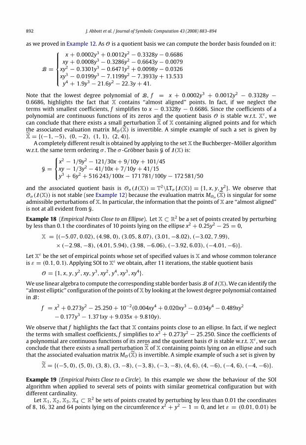
as we proved in Example 12. As O is a quotient basis we can compute the border basis founded on it:

B =

x + 0.0002y3 + 0.0012y2 − 0.3328y− 0.6686xy + 0.0008y3 − 0.3286y2 − 0.6643y− 0.0079xy2 − 0.3301y3 − 0.6471y2 + 0.0098y− 0.0326xy3 − 0.0199y3 − 7.1199y2 − 7.3933y+ 13.533y4 + 1.9y3 − 21.6y2 − 22.3y+ 41.

Note that the lowest degree polynomial of B, f = x + 0.0002y3 + 0.0012y2 − 0.3328y −0.6686, highlights the fact that X contains ‘‘almost aligned’’ points. In fact, if we neglect theterms with smallest coefficients, f simplifies to x − 0.3328y − 0.6686. Since the coefficients of apolynomial are continuous functions of its zeros and the quotient basis O is stable w.r.t. Xε , wecan conclude that there exists a small perturbation X of X containing aligned points and for whichthe associated evaluation matrix MO(X) is invertible. A simple example of such a set is given byX = {(−1,−5), (0,−2), (1, 1), (2, 4)}.A completely different result is obtained by applying to the setX the Buchberger–Möller algorithm

w.r.t. the same term ordering σ . The σ -Gröbner basis G of I(X) is:

G =

x2− 1/9y2 − 121/30x+ 9/10y+ 101/45

xy − 1/3y2 − 41/10x+ 7/10y+ 41/15y3 + 6y2 + 516 243/100x− 171 781/100y− 172 581/50

and the associated quotient basis is Oσ (I(X)) = T2\LTσ {I(X)} = {1, x, y, y2}. We observe thatOσ (I(X)) is not stable (see Example 12) because the evaluation matrix MOσ (X) is singular for someadmissible perturbations of X. In particular, the information that the points of X are ‘‘almost aligned’’is not at all evident from G.

Example 18 (Empirical Points Close to an Ellipse). Let X ⊂ R2 be a set of points created by perturbingby less than 0.1 the coordinates of 10 points lying on the ellipse x2 + 0.25y2 − 25 = 0,

X = {(−5.07, 0.02), (4.98, 0), (3.05, 8.07), (3.01,−8.02), (−3.02, 7.99),× (−2.98,−8), (4.01, 5.94), (3.98,−6.06), (−3.92, 6.03), (−4.01,−6)}.

Let Xε be the set of empirical points whose set of specified values is X and whose common toleranceis ε = (0.1, 0.1). Applying SOI to Xε we obtain, after 11 iterations, the stable quotient basis

O = {1, x, y, y2, xy, y3, xy2, y4, xy3, xy4}.

Weuse linear algebra to compute the corresponding stable border basisB ofI(X).We can identify the‘‘almost elliptic’’ configuration of the points ofX by looking at the lowest degree polynomial containedinB:

f = x2 + 0.273y2 − 25.250+ 10−2(0.004xy4 + 0.020xy3 − 0.034y4 − 0.489xy2

− 0.177y3 − 1.371xy+ 9.035x+ 9.810y).

We observe that f highlights the fact that X contains points close to an ellipse. In fact, if we neglectthe terms with smallest coefficients, f simplifies to x2 + 0.273y2 − 25.250. Since the coefficients ofa polynomial are continuous functions of its zeros and the quotient basis O is stable w.r.t. Xε , we canconclude that there exists a small perturbation X of X containing points lying on an ellipse and suchthat the associated evaluation matrixMO(X) is invertible. A simple example of such a set is given by

X = {(−5, 0), (5, 0), (3, 8), (3,−8), (−3, 8), (−3,−8), (4, 6), (4,−6), (−4, 6), (−4,−6)}.

Example 19 (Empirical Points Close to a Circle). In this example we show the behaviour of the SOIalgorithm when applied to several sets of points with similar geometrical configuration but withdifferent cardinality.Let X1,X2,X3,X4 ⊂ R2 be sets of points created by perturbing by less than 0.01 the coordinates

of 8, 16, 32 and 64 points lying on the circumference x2 + y2 − 1 = 0, and let ε = (0.01, 0.01) be


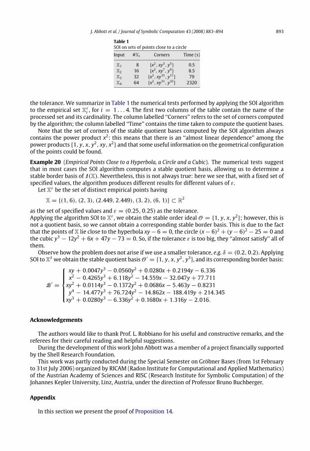
Table 1SOI on sets of points close to a circleInput #Xi Corners Time (s)

X1 8 {x2, xy3, y5} 0.5X2 16 {x2, xy7, y9} 8.5X3 32 {x2, xy15, y17} 79X4 64 {x2, xy31, y33} 2320

the tolerance. We summarize in Table 1 the numerical tests performed by applying the SOI algorithmto the empirical set Xεi , for i = 1 . . . 4. The first two columns of the table contain the name of theprocessed set and its cardinality. The column labelled ‘‘Corners’’ refers to the set of corners computedby the algorithm; the column labelled ‘‘Time’’ contains the time taken to compute the quotient bases.Note that the set of corners of the stable quotient bases computed by the SOI algorithm always

contains the power product x2: this means that there is an ‘‘almost linear dependence’’ among thepower products {1, y, x, y2, xy, x2} and that some useful information on the geometrical configurationof the points could be found.

Example 20 (Empirical Points Close to a Hyperbola, a Circle and a Cubic). The numerical tests suggestthat in most cases the SOI algorithm computes a stable quotient basis, allowing us to determine astable border basis of I(X). Nevertheless, this is not always true: here we see that, with a fixed set ofspecified values, the algorithm produces different results for different values of ε.Let Xε be the set of distinct empirical points having

X = {(1, 6), (2, 3), (2.449, 2.449), (3, 2), (6, 1)} ⊂ R2

as the set of specified values and ε = (0.25, 0.25) as the tolerance.Applying the algorithm SOI to Xε , we obtain the stable order ideal O = {1, y, x, y2}; however, this isnot a quotient basis, so we cannot obtain a corresponding stable border basis. This is due to the factthat the points of X lie close to the hyperbola xy− 6 = 0, the circle (x− 6)2 + (y− 6)2 − 25 = 0 andthe cubic y3 − 12y2 + 6x+ 47y− 73 = 0. So, if the tolerance ε is too big, they ‘‘almost satisfy’’ all ofthem.Observe how the problem does not arise if we use a smaller tolerance, e.g. δ = (0.2, 0.2). Applying

SOI toXδ we obtain the stable quotient basisO′ = {1, y, x, y2, y3}, and its corresponding border basis:

B ′ =

xy + 0.0047y3 − 0.0560y2 + 0.0280x+ 0.2194y− 6.336x2 − 0.4265y3 + 6.118y2 − 14.559x− 32.047y+ 77.711xy2 + 0.0114y3 − 0.1372y2 + 0.0686x− 5.463y− 0.8231y4 − 14.477y3 + 76.724y2 − 14.862x− 188.419y+ 214.345xy3 + 0.0280y3 − 6.336y2 + 0.1680x+ 1.316y− 2.016.

Acknowledgements

The authors would like to thank Prof. L. Robbiano for his useful and constructive remarks, and thereferees for their careful reading and helpful suggestions.During the development of this work John Abbott was a member of a project financially supported

by the Shell Research Foundation.This work was partly conducted during the Special Semester on Gröbner Bases (from 1st February

to 31st July 2006) organized by RICAM (Radon Institute for Computational and Applied Mathematics)of the Austrian Academy of Sciences and RISC (Research Institute for Symbolic Computation) of theJohannes Kepler University, Linz, Austria, under the direction of Professor Bruno Buchberger.

Appendix

In this section we present the proof of Proposition 14.


Proof. First we prove a simple result about the homogeneous components of degrees 0 and 1 ofthe inverse of a matrix. Let A be a non-singular element of Matc×c(F), and let B be its inverse. Thehomogeneous components B0 and B1 are given by

B0 = A−10 B1 = −A−10 A1A−10 = −B0A1B0. (9)

We show this by decomposing A and B into sums of homogeneous components:

A = A0 + A1 + A2+ and B = B0 + B1 + B2+

where A2+ =∑i≥2 Ai and B2+ =

∑i≥2 Bi. Now, since AB = I , the c × c identity matrix, we have

(A0 + A1 + A2+)(B0 + B1 + B2+) = I

and our claim is immediate after expanding the product into a sum of homogeneous components.Now we prove the result of the proposition. Since M is a full rank matrix, the matrix A = M tM is

non-singular and so we can define

α = A−1M tv (10)ρ = v −Mα. (11)

Applying to (11) the homogeneous degree decomposition up to degree 1 we have

ρ0 + ρ1 = (v0 −M0α0)+ (v1 −M0α1 −M1α0)

thus (4) follows.Since A0 = M t0M0 and A1 = M

t0M1 +M

t1M0, from formula (9) we have the first two homogeneous

components of B = A−1 ≡ A−10 − A−10 A1A

−10 . Up to degree 1, formula (10) becomes

α0 + α1 = B0(M t0v0 +Mt0v1 +M

t1v0)+ B1M

t0v0 = B0

(M t0v0 +M

t0v1 +M

t1v0 − A1B0M

t0v0

)and so

α0 = (M t0M0)−1M t0v0

α1 = (M t0M0)−1(M t0v1 +M

t1v0 −M

t0M1α0 −M

t1M0α0)

thus the proof is concluded. �

References

Abbott, J., Bigatti, A., Kreuzer, M., Robbiano, L., 2000. Computing ideals of points. J. Symbolic. Comput. 30, 341–356.Abbott, J., 2007. Twin-float arithmetic (submitted for publication).Abbott, J., Fassino, C., Torrente, M., 2007. Thinning out redundant empirical data. Math. Comput. Sci. 1 (2), 375–392.Buchberger, B., Möller, H.M., 1982. The construction of multivariate polynomials with preassigned zeros. In: Proc. EUROCAM’82. In: LNCS, vol. 144. pp. 24–31.

CoCoA Team, 0000. CoCoA: A system for doing computations in commutative algebra. Available at: http://cocoa.dima.unige.it/.Dahlquist, G., Björck, Å., Anderson, N., 1974. Numerical Methods. Englewood Cliffs, New Jersey.Demmel, J.W., Higham, N.J., 1993. Improved error bounds for underdetermined system solvers. SIAM J. Matrix Anal. Appl. 14,1–14.

Heldt, D., Kreuzer, M., Pokutta, S., Poulisse, H., 2006. Approximate computation of zero-dimensional polynomial ideals. Preprintavailable on line at: http://staff.fim.uni-passau.de/algebraic-oil/en/Publications/index.html.

Kreuzer, M., Robbiano, L., 2000. Computational Commutative Algebra 1. Springer-Verlag, Berlin.Kreuzer, M., Robbiano, L., 2005. Computational Commutative Algebra 2. Springer-Verlag, Berlin.Kehrein, A., Kreuzer,M., Robbiano, L., 2005. An algebraist’s viewonborder bases. In: Solving Polynomial Equations: Foundations,Algorithms, and Applications, Proc. CIMPA School (Buenos Aires 2003). Springer-Verlag, Heidelberg.

Mourrain, B., Ruatta, O., 2002. Relation between roots and coefficients, interpolation and application to system solving. J.Symbolic. Comput. 33 (5), 679–699.

Mourrain, B., Trébuchet, Ph., 2005. Generalizednormal forms andpolynomial systemsolving. In: Proc. Intern. Symp. on Symbolicand Algebraic Computation. pp. 253–260.

Mourrain, B., 2007. Pythagore’s dilemma, symbolic-numeric computation, and the border basis method. Symbolic-NumericComputations (Trends in Mathematics) 223–243.

Sauer, T., 2007. Approximate varieties, approximate ideals and dimension reductions. Numerical Algorithms 45, 295–313.Stetter, H.J., 2004. Numerical Polynomial Algebra. SIAM, Philadelphia, PA, USA.

http://cocoa.dima.unige.it/

http://staff.fim.uni-passau.de/algebraic-oil/en/Publications/index.html

Documents

Stable border bases for ideals of points