Embed Size (px)
Citation preview

Universitat Ulm
Fakultat fur Mathematik und
Wirtschaftswissenschaften
Stable Implementation of
Three-Term Recurrence Relations
Bachelorarbeit
in Mathematik
vorgelegt von
Pascal Frederik Heiter
am 14. Juni 2010
Gutachter
Prof. Dr. Stefan A. Funken

Acknowledgement. First of all, I would like to thank my advisor, Prof. Dr.
Stefan A. Funken, for his support, instructions and patience during my work. I
achieved an interesting insight in mathematical research.
Moreover, I would like to thank Andreas Bantle for his strenuous efforts to support
me, whenever I needed help, and for editing my thesis. Special thanks to Markus
Bantle and Christoph Erath for answering many questions.
Last but not least I would like to thank my parents. Without their support, it would
never have been possible to write this thesis.
Ulm, June 2010.

Contents
1 Introduction 1
1.1 Motivation 1
1.2 Aim of this Thesis 3
1.3 Outline 3
2 Three-Term Recurrence Relations 5
2.1 Legendre Polynomials and Functions 5
2.2 Three-Term Recurrence Relation 7
2.3 Special Cases of Three-Term Recurrence Relations 11
2.4 Computation of Initial Values 16
3 Stable Numerical Calculation of Minimal Solutions 25
3.1 Forward Evaluation 26
3.2 Miller’s Backward Algorithm 28
3.3 Gautschi’s Continued Fraction Algorithm 31
3.4 Estimate of ν as Against Adaptive Determination 33
3.5 Error Analysis and Ellipse Parameters 35
4 C-Library ’liblegfct.c’ 41
4.1 The Function qtm1 42
4.2 The Function q0 47
4.3 The Function qtn 48
4.4 Test Files 51
5 Conclusion 59
A The file ’liblegfct.h’ 61
B The file ’liblegfct.c’ 69
C Result of all test files 97


Chapter 1
Introduction
1.1 Motivation
Three-term recurrence relations become significant and useful in numerical
mathematics, especially for the calculation of orthogonal polynomials such as
Tschebyscheff, Jacobi, Laguerre, Hermite and Legendre polynomials. There exist
different types of solutions of three-term recurrence relation, for example minimal
and dominant solutions. However, the computation of a minimal solution by a given
three-term recurrence relation is in general numerically instable, which is demon-
strated by the following example.
Example 1.1.1 We consider
Qk(x) :=1
2
1∫
−1
Pk(t)
x− tdt , x ∈ R , k ∈ N0,
where Pk(x) is the Legendre polynomial of degree k. The main aim is the calculation
of these integrals for k = 0, 1 . . . n. One possible solution is to calculate the partial
fraction and integrate elementary functions, but the effort is too high. An alternative
way to compute these integrals is given by the computation via the following three-
term recurrence relations. It is desirable to have a fast, efficient and stable method.
The Qk(x), also called Legendre functions, satisfy the same recurrence relation as the
Legendre polynomials. There are no problems to evaluate this three-term recurrence
relation for x ∈ [−1, 1] as depicted in Figure 1.1 for k = 30.
As we see in Figure 1.2, the computation for |x| > 1 and k ≫ 1 contrasts the
analytical fact, that limk→∞Qk(x) = 0 (|x| > 1). We can study the beginning of the
oscillation, particularly the point, from which the relative error is larger than a given
tolerance. Taking a look at the calculation of Qk(z) with z ∈ C, we notice that the
points, from which the oscillation begins, are located around an ellipse respecting
to the real interval [−1, 1], see also Chapter 3.
There are known several algorithms calculating numerically stable a minimal solu-
tion for a three-term recurrence relation, e.g. Miller’s backward algorithm, Olver’s
algorithm and Gautschi’s continued fraction algorithm, to name a few, but not all.
Gautschi discusses three-term recurrence relations intensively in [5] and [6]. In [11]

2 Chapter 1: Introduction
−1 −0.5 0 0.5 1−0.8
−0.6
−0.4
−0.2
0
0.2
0.4
0.6
0.8
Figure 1.1: Q30(x) computed with a three-term recurrence relation for x ∈ [−1, 1].
0.6 0.8 1 1.2 1.4 1.6 1.8
−3
−2.5
−2
−1.5
−1
−0.5
0
0.5
1
1.5
Figure 1.2: Q30(x) computed with a three-term recurrence relation for x ∈ [0.5, 1.8].
Zhang and Jin present an algorithm to determine Qk(z). However, this algorithm
is in general not stable yet.
An important application of three-term recurrence relations is the numerics of par-
tial differential equations. As against many cases, in which it is just possible to
solve the partial differential equation numerically, in a few cases, they can be solved
analytically. There are various numerical ways to solve PDEs, e.g. with the finite
element method or the boundary element method. Integral operators that occur in
the boundary element method can be resolved to elementary integrals, which can
be compute by three-term recurrence relations, see [1].
This thesis is embedded in a project, which deals with the efficient p-stablized im-
plementation of the boundary element method. The results of this thesis allow us

Section 1.2: Aim of this Thesis 3
to create a useful library including many functions to compute integrals of the type
1∫
−1
log |x− y|Pk(y)dy,
where Pk(y) is the Legendre polynomial of degree k. We optimize Gautschi’s con-
tinued fraction algorithm and use this algorithm to stabilize the calculation. We
suggest to calculate these minimal solution with C functions instead of calculation
with Matlab, because in C we reach more performance through parallelization e.g.
via OpenMP orNVIDIA CUDA. Interfaces between Matlab and C are required,
however there are not discuss in this work, see [2].
1.2 Aim of this Thesis
The aim of this work is to gain an efficient, fast and stable method to compute min-
imal solutions of three-term recurrence relations. The focus is on the investigation
of three-term recurrence relations, the analysis of the area of instability, especially
the assignment of the specific ellipse parameter and the stable implementation and
the detailed description of the implementation.
1.3 Outline
The thesis is structured into five main chapters.
A short overview of the Legendre polynomials and functions is given in Chapter 2 as
an example for a three-term recurrence relation. Furthermore, the second chapter
contains the theory of three-term recurrence relations and special cases with the
related initial values.
Chapter 3 deals with the stable numerical calculation of minimal solutions and intro-
duces two algorithms, namely Miller’s backward algorithm and Gautschi’s continued
fraction algorithm, stabilizing the computation of these solutions. The error analysis
and the optimization of the Gautschi’s continued fraction algorithm is discussed in
the end of Chapter 3.
Chapter 4 includes a detailed description of the created C-Library ’liblegfct.c’ and
several test methods.

4 Chapter 1: Introduction
Chapter 2
Three-Term Recurrence Relations
In order to define some integrals, we give a short overview of Legendre functions
and their properties. Afterwards, we take a look at three-term recurrence relations
and prove, that the integrals, we defined before, satisfy three-term recurrence rela-
tions. In fact, we gain a method to compute these integrals without being forced
to integrate all terms. In the end of this chapter, we calculate the initial values of
these three-term recurrence relations.
2.1 Legendre Polynomials and Functions
The differential equation
(1− z2)d2
dz2u(z)− 2z
d
dzu(z) + k(k + 1)u(z) = 0 , k ∈ N0, (2.1)
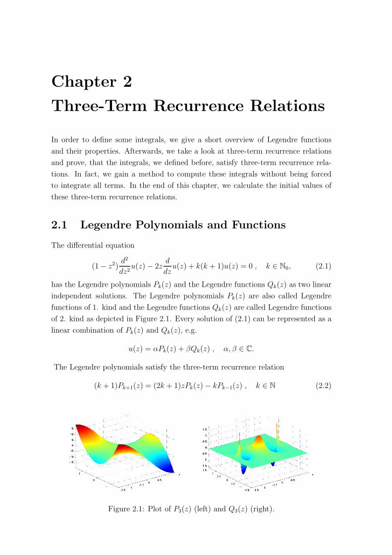
has the Legendre polynomials Pk(z) and the Legendre functions Qk(z) as two linear
independent solutions. The Legendre polynomials Pk(z) are also called Legendre
functions of 1. kind and the Legendre functions Qk(z) are called Legendre functions
of 2. kind as depicted in Figure 2.1. Every solution of (2.1) can be represented as a
linear combination of Pk(z) and Qk(z), e.g.
u(z) = αPk(z) + βQk(z) , α, β ∈ C.
The Legendre polynomials satisfy the three-term recurrence relation
(k + 1)Pk+1(z) = (2k + 1)zPk(z)− kPk−1(z) , k ∈ N (2.2)
Figure 2.1: Plot of P3(z) (left) and Q3(z) (right).

6 Chapter 2: Three-Term Recurrence Relations
which is well conditioned for z ∈ R, |z| < 1 and with the initial values
P0(z) = 1, P1(z) = z.
The Rodrigues formula
Pk(z) =1
2kk!
dk
dzk(z2 − 1) , k ∈ N0
is an alternative to represent the Legendre polynomials. Special cases of Pk(z) are
P0(z) = 1, P3(z) = 12(5z3 − 3z),
P1(z) = z, P4(z) = 18(35z4 − 30z2 + 3),
P2(z) = 12(3z2 − 1), P5(z) = 1
8(63z5 − 70z3 + 15z).
The Legendre functions of 2. kind also satisfy the three-term recurrence relation
(2.2). Another representation formula is given by
Qk(z) =1
2log
(z + 1
z − 1
)
Pk(z)−Wk−1(z),
whereas the Wk(z) satisfy the three-term recurrence relation
(k + 1)Wk(z) = (2k + 1)zWk−1(z)− kWk−2(z) , k ∈ N
with the initial values W−1 = 0, W0 = 1. The functions Wk(z) can be calculated
without the previous three-term recurrence relation as well via
Wk−1(z) =k∑
m=1
1
mPm−1(z)Pk−m(z).
Special cases of Qk(z) are
Q0(z) = 12log(z+1z−1
)= 1
2P0(z) log
(z+1z−1
),
Q1(z) = z · 12log(z+1z−1
)− 1 = 1
2P1(z) log
(z+1z−1
)−W0(z),
Q2(z) = 12(3z2 − 1) · 1
2log(z+1z−1
)− 3
2z = 1
2P2(z) log
(z+1z−1
)−W1(z).
The associated Legendre functions of 2. kind are defined for x ∈ [−1, 1] as
Qmk (x) = (−1)m(1− x2)
m2dm
dxmQk(x) , m ∈ N0,
and for the general case z ∈ C as
Qmk (z) = (z2 − 1)
m2dm
dzmQk(z) , m ∈ N0.
Note, thatQk(z) = Q0k(z) and for further information, see [7]. Some useful properties
of the Legendre functions are given in the following lemma.

Section 2.2: Three-Term Recurrence Relation 7
Lemma 2.1.1 (i) There holds for the antiderivatives
t∫
−1
Pk(ξ)dξ =1
2k + 1(Pk+1(t)− Pk−1(t)) , k ∈ N.
(ii) There holds for the derivatives
d
dzPk(z) =
k(k + 1)
2k + 1
Pk+1(t)− Pk−1(t)
z2 − 1, k ∈ N.
(iii) There holds
(Pk+1 − Pk−1)(±1) = 0 , k ∈ N.
(iv) Based on the orthogonality of Pk(t), there holds
1∫
−1
Pk(t)Pm(t)dt =
0, k 6= m
22k+1
, k = m
(v) For | arg(z − 1)| < π we have the following relation between the Legendre
functions of 1. and 2. kind
Qk(z) =1
2
1∫
−1
Pk(z)
z − tdt , k ∈ N0.
(vi) There holds the functional relations over m and for x ∈ [−1, 1]
Qm+2k (x) =
−2(m+ 1)x√1− x2
Qm+1k (x)− (k +m+ 1)(k −m)Qm
k (x)
and for the general case z ∈ C, there holds the three-term recurrence relation
over m
Qm+2k (z) =
−2(m+ 1)z√z2 − 1
Qm+1k (z) + (k +m+ 1)(k −m)Qm
k (z).
Proof. See [7] and [8].
2.2 Three-Term Recurrence Relation
In the following we want to investigate three-term recurrence relations. A three-
term recurrence relation is a specification how to compute a new value with the two
previous values. There are two different types of three-term recurrence relation. An
inhomogeneous three-term recurrence relation is defined as
yn+1 = anyn + bnyn−1 + cn (2.3)

8 Chapter 2: Three-Term Recurrence Relations
and a uniform three-term recurrence relation is defined as
yn+1 = anyn + bnyn−1 (2.4)
whereas an, bn, cn ∈ C are arbitrary numbers. The most popular example for a
three-term recurrence relation is the Fibonacci numbers.
Example 2.2.1 The Fibonacci numbers satisfy the three-term recurrence relation
Fn+1 = Fn + Fn−1 , n ∈ N
with the initial values F0 = 0 and F1 = 1.
The first values are
F0 F1 F2 F3 F4 F5 F6 F7 F8 F9 F10 . . .
0 1 1 2 3 5 8 13 21 34 55 . . . .
Note, that this three-term recurrence relation is uniform, see Equation (2.4) with
an = bn = 1.
Given a three-term recurrence relation
(k−n+1)fk+1+s(z) = (2k+1)zfk+s(z)−(k+n)fk−1+s(z) , k ∈ N, s, n ∈ Z, (2.5)
we want to transform these relation to gain a modified formula, such that the leading
coefficients of all fk+s(z) are equal to one. This property is required by Gautschi’s
continued fraction algorithm, which is discussed in Chapter 3.
Lemma 2.2.2 Let n, s ∈ Z, fk+s(z) (k ∈ N0) satisfy (2.5) and
fk+s(z) :=
k∏
j=2
j − n
2j − 1fk+s(z).
Then there holds the three-term recurrence relation
fk+1+s(z) = zfk+s(z)− bkfk−1+s(z) , k ∈ N, (2.6)
with
bk+s =(k − n)(k + n)
(2k − 1)(2k + 1).
Proof. We take a look at the leading coefficients of fk
f0+s(z) = 1
f1+s(z) = z
f2+s(z) =3
2− nzf1+s(z) + (1 + n)f0+s(z) =
3
2− nz2 + . . .

Section 2.2: Three-Term Recurrence Relation 9
f3+s(z) =5
3− nzf2+s(z) + (2 + n)f1+s(z) =
3 · 5(2− n)(3− n)
z3 + . . .
f4+s(z) =7
4− nzf3+s(z) + (3 + n)f2+s(z) =
3 · 5 · 7(2− n)(3− n)(4− n)
z4 + . . .
...
and obtain
fk+s(z) =
k∏
j=2
2j − 1
j − nzk −
k−1∑
m=0
αmzm. (2.7)
We prove (2.7) by induction on k. For the initial step with k = 0, there holds
f0+s(z) =0∏
j=2
j − n
2j − 1f0+s(z) = 1.
Let (2.7) be true for an arbitrary k ∈ N, but fixed. Then there holds by using the
induction hypothesis (2.7)
(k + 1− n)fk+1+s(z) = (2k + 1)zfk+s(z)− (k + n)fk−1+s(z)
= (2k + 1)z
(k∏
j=2
2j − 1
j − nzk −
k−1∑
m=0
αmzm
)
− (k + n)fk−1+s(z)
= (2k + 1)
k∏
j=2
2j − 1
j − nzk+1 − (2k + 1)
k−1∑
m=0
αmzm+1 − (k + n)fk−1+s(z)
This is equivalent to
fk+1+s(z) =2k + 1
k + 1− n
k∏
j=2
2j − 1
j − nzk+1 − 2k + 1
k + 1− n
k−1∑
m=0
αmzm+1 − k + n
k + 1− nfk−1+s(z)
︸ ︷︷ ︸
=:∑k
m=0 βmzm
=k+1∏
j=2
2j − 1
j − nzk+1 −
k∑
m=0
βmzm.
To get a leading coefficient one, we have to multiply fk+1+s(z) by∏k+1
j=2j−n
2j−1. This
leads to
fk+s(z) =
k∏
j=2
j − n
2j − 1fk+s(z).
Now, we prove the three-term recurrence relation (2.6). Let
dk+s =Πk
j=1(2j − 1)
Πki=2(i− n)
.

10 Chapter 2: Three-Term Recurrence Relations
Then there holds
dk+1+sfk+1+s(z) = fk+1+s(z) =2k + 1
k + 1− nzfk+s(z) +
k + n
k + 1− nfk−1+s(z)
=2k + 1
k + 1− ndkzfk+s(z) +
k + n
k + 1− ndk−1fk−1+s(z)
= dk+1+szfk+s(z) +k + n
k + 1− ndk−1+sfk−1+s(z).
By dividing the last equation by dk+1+s, we get
fk+1+s(z) = zfk+s(z) +k + n
k + 1− n
dk−1+s
dk+1+s
fk−1+s(z)
= zfk+s(z) +(k + n)(k − n)
(2k − 1)(2k + 1)fk−1+s(z),
which proves the assumption.
Remark 2.2.3 Let k ∈ N0, s ∈ Z, f0+s(z) = 1 and f1+s(z) = z. Then fk+s(z) is a
polynomial and the leading coefficient is equal to one.
We will prove several three-term recurrence relation in the next chapter. To simplify
the corresponding proofs, we show the following lemma.
Lemma 2.2.4 Let fk(z) satisfy (2.5) and
gk+s(z) :=fk+1(z)− fk−1(z)
2k + 1.
Then there holds the three-term recurrence relation
(k − n+ 2)gk+1+s(z) = (2k + 1)zgk+s(z)− (k + n− 1)gk−1+s(z) , k ∈ N, s, n ∈ Z.
Proof. By using the definition of gk+s(z) and the three-term recurrence relation of
fk(z), we obtain
gk+1+s(z) =fk+2(z)− fk(z)
2k + 3
=1
2k + 3
(2k + 3
k − n+ 2zfk+1 −
k + 1 + n
k − n + 2fk(z)− fk(z)
)
=1
2k + 3
(2k + 3
k − n+ 2zfk+1 −
2k + 3
k − n + 2fk(z)
)
=1
k − n + 2(zfk+1 − fk(z)) .

Section 2.3: Special Cases of Three-Term Recurrence Relations 11
We expand the last term with ±zfk−1(z), use the three-term recurrence relation of
fk(z) again, and obtain
gk+1+s(z) =1
k − n+ 2(zfk+1 − zfk−1(z) + zfk−1(z)− fk(z))
=1
k − n+ 2
(
z(fk+1 − fk−1(z)) +k − n
2k − 1fk(z)− fk(z)
+k + n− 1
2k − 1fk−2(z)
)
=1
k − n+ 2
(
z(fk+1 − fk−1(z))−k + n− 1
2k − 1fk(z)−
k + n− 1
2k − 1fk−2(z)
)
=1
k − n+ 2
(
z(fk+1 − fk−1(z))−k + n− 1
2k − 1(fk(z)− fk−2(z))
)
.
In the end, we have to use the definition of gk+s(z) and get
gk+1+s(z) =1
k − n+ 2((2k + 1)zgk+s(z)− (k + n− 1)gk−1+s(z)) ,
which is equivalent to
(k − n+ 2)gk+1+s(z) := (2k + 1)zgk+s(z)− (k + n− 1)gk−1+s(z).
2.3 Special Cases of Three-Term Recurrence Re-
lations
Let Pk(x) be the Legendre polynomial with degree k. We use the notations
Q−1k (z) :=
1∫
−1
Pk(t) log(t− z)dt , k ∈ N0 (2.8)
Qmk (z) :=
1∫
−1
Pk(t)
(z − t)m+1dt , k,m ∈ N0 (2.9)
Nk(t) :=
12(P0(t)− P1(t)) k = 1
12(P0(t) + P1(t)) k = 2∫ t
−1Pk(ξ)dξ k > 2
(2.10)
R−1k (z) :=
1∫
−1
Nk(t) log(t− z)dt , k ∈ N (2.11)
Rmk (z) :=
1∫
−1
Nk(t)
(z − t)m+1dt , k ∈ N, m ∈ N0. (2.12)

12 Chapter 2: Three-Term Recurrence Relations
In the following, we prove, that the functions, we defined above, satisfy three-term
recurrence relations. In fact, we gain a fast method evaluating integrals with a
complexity of O(n).
2.3.1 Three-Term Recurrence Relation for Qm
k(z)
Remember the definitions
Q−1k (z) :=
1∫
−1
Pk(t) log(t− z)dt , k ∈ N0,
Qmk (z) :=
1∫
−1
Pk(t)
(z − t)m+1dt , k,m ∈ N0.
In the following lemma, we give a useful property of Qmk (z) and describe the relation
between Qmk (z) an Qm
k (z).
Lemma 2.3.1 Let z ∈ C\{±1}.
(i) There holds the relation between Qmk and Qm
k
Qmk (z) =
(z2 − 1)m2
2· (−1)mm!Qm
k , k ∈ N0, m ∈ N.
(ii) There holds the relation between Qmk and Qm+1
k
Qmk (z) =
−(m+ 1)
2k + 1(Qm+1
k+1 (z)− Qm+1k−1 (z)) , k ∈ N, m ∈ N0 ∪ {−1}.
Proof. ad (i) The definition of Qmk (z) and property (v) of Lemma 2.1.1 leads to
Qmk (z) = (z2 − 1)
m2dm
dzmQk(z) =
(z2 − 1)m2
2
dm
dzm
1∫
−1
Pk(t)
z − tdt.
By derivating m times, we get
Qmk (z) =
(z2 − 1)m2
2
dm
dzm
1∫
−1
Pk(t)
z − tdt
=(z2 − 1)
m2
2· (−1)mm!
1∫
−1
Pk(t)
(z − t)m+1dt
=(z2 − 1)
m2
2· (−1)mm!Qm
k .

Section 2.3: Special Cases of Three-Term Recurrence Relations 13
ad (ii) Let m > −1. We use integration by parts and get
Qmk (z) =
1∫
−1
Pk(t)
(z − t)m+1dt
=
t∫
−1
Pk(ξ)dξ ·1
(z − t)m+1
∣∣∣∣∣∣
1
−1︸ ︷︷ ︸
=0
−1∫
−1
t∫
−1
Pk(ξ)dξ
· m+ 1
(z − t)m+2dt.
Using property (i) of Lemma 2.1.1, we obtain
Qmk (z) = −
1∫
−1
1
2k + 1(Pk+1(t)− Pk−1(t))
m+ 1
(z − t)m+2dt
= −m+ 1
2k + 1
1∫
−1
Pk+1(t)− Pk−1(t)
(z − t)m+2 dt
=−(m+ 1)
2k + 1
(
Qm+1k+1 (z)− Qm+1
k−1 (z))
.
The proof for m = −1 can be done similarly.
The three-term recurrence relation for Qmk (z) is considered in the next theorem. The
initial values are given in Chapter 2.4.
Lemma 2.3.2 Let m ∈ N0 ∪ {−1} and Qmk (z) as defined above. Then there holds
the three-term recurrence relation over k
(k −m+ 1)Qmk+1(z) = (2k + 1)zQm
k (z)− (k +m)Qmk−1(z) , k ≥ 1
and another three-term recurrence relation over m
Qm+1k (z) =
2mz
(z2 − 1)(m+ 1)Qm
k (z)+(k +m)(k −m+ 1)
(z2 − 1)(m+ 1)mQm−1
k (z) , m ∈ N, k ∈ N0
with the initial values as in Lemma 2.4.3. Note, that for m = −1, the first three-term
recurrence relation only holds for k > 1.
Proof. Let k ≥ 1. Then there holds by using the three-term recurrence relation for
Legendre polynomials
Qmk+1(z) =
1∫
−1
Pk+1(t)
(z − t)m+1dt
=1
k + 1
1∫
−1
(2k + 1)tPk(t)− kPk−1(t)
(z − t)m+1 dt.

14 Chapter 2: Three-Term Recurrence Relations
We expand tPk(t) with ±zPk(t) and obtain for the last equation
Qmk+1(z) =
2k + 1
k + 1
1∫
−1
(t− z + z)Pk(t)
(z − t)m+1 dt
− k
k + 1
1∫
−1
Pk−1(t)
(z − t)m+1dt
=2k + 1
k + 1
−1∫
−1
Pk(t)
(z − t)mdt+ z
1∫
−1
Pk(t)
(z − t)m+1dt
− k
k + 1
1∫
−1
Pk−1(t)
(z − t)m+1dt
=2k + 1
k + 1
−1∫
−1
Pk(t)
(z − t)mdt+ zQm
k (z)
− k
k + 1Qm
k−1(z).
To complete the proof, we need the result of the previous Lemma 2.3.1 and obtain
Qmk+1(z) =
2k + 1
k + 1
(
− −m
2k + 1
(
Qmk+1(z)− Qm
k−1(z))
+ zQmk (z)
)
− k
k + 1Qm
k−1(z)
=m
k + 1Qm
k+1(z)−m
k + 1Qm
k−1(z) +2k + 1
k + 1zQm
k (z)−k
k + 1Qm
k−1(z).
Thus we have
(k + 1)Qmk+1(z)−mQm
k+1(z) = (2k + 1)zQmk (z)−mQm
k−1(z)− kQmk−1(z)
and
(k + 1−m)Qmk+1 = (2k + 1)zQm
k (z)− (k +m)Qmk−1(z).
The proof for Q−1k+1(z) can be done similarly. The three-term recurrence relation for
Qmk (z) over m can be proved by using Lemma 2.3.1 and Lemma 2.1.1 (vi).
Remark 2.3.3 The three-term recurrence relation for Qmk (z) is a special case of
(2.5) with s = 0 and n = m.
2.3.2 Three-Term Recurrence Relation for Nk(t)
Remember the definition
Nk(t) =
12(P0(t)− P1(t)), k = 1,
12(P0(t) + P1(t)), k = 2,∫ t
−1Pk(ξ)dξ, k > 2.
Lemma 2.3.4 Let Nk(t) as defined above. Then there holds
(i) N1(t) =12(1− t)
(ii) N2(t) =12(1 + t)

Section 2.3: Special Cases of Three-Term Recurrence Relations 15
(iii) The Nk(t) satisfies the three-term recurrence relation
(k + 2)Nk+3(t) = (2k + 1)tNk+2(t)− (k − 1)Nk+1(t) , k ≥ 2
with N3(t) =12(t2 − 1) and N4(t) =
12(t3 − t).
Note, that the Nk(t) are called Lobatto shape functions.
Proof. We notice the relation
Nk(t) =1
2k − 3(Pk−1(t)− Pk−3(t)) , k ≥ 3
based on property (i) of Lemma 2.1.1. The Legendre polynomials satisfy (2.5). We
define
gk+2(z) := Nk(t) , k ∈ N
use Lemma 2.2.4 with s = 2, n = 0 and complete the proof. The initial values are
treaded in Lemma 2.4.4.
Remark 2.3.5 The three-term recurrence relation for Nk(t) is a special case of
(2.5) with s = 2 and n = −1.
2.3.3 Three-Term Recurrence Relation for Rm
k(z)
Remember the definitions
R−1k (z) :=
1∫
−1
Nk(t) log(t− z)dt , k ∈ N,
Rmk (z) :=
1∫
−1
Nk(t)
(z − t)m+1dt , k ∈ N, m ∈ N0.
We investigate the relation between Rmk (z) and Qm
k (z).
Lemma 2.3.6 Let m ∈ N0 ∪ {−1}. There holds the following relation between
Rmk (z) and Qm
k (z)
Rmk+2(z) =
1
2k + 1(Qm
k+1(z)− Qmk−1(z)) , k ∈ N.
Proof. Let m ∈ N0. Based on the definitions of Rmk (z) and Nk(t) and property (i)

16 Chapter 2: Three-Term Recurrence Relations
of Lemma 2.1.1, we get
Rmk+2(z) =
1∫
−1
Nk+2(t)
(z − t)m+1dt
=
1∫
−1
Pk+1(t)− Pk−1(t)
2k + 1
1
(z − t)m+1dt
=1
2k + 1
1∫
−1
Pk+1(t)
(z − t)m+1dt−
1∫
−1
Pk−1(t)
(z − t)m+1dt
=1
2k + 1
(
Qmk+1(z)− Qm
k−1(z))
.
The proof for m = −1 can be done similarly.
The last lemma allows us to simplify the proof of the three-term recurrence relation
for Rmk (z).
Lemma 2.3.7 Let m ∈ N0 ∪ {−1} and Rmk (z) as defined above. Then there holds
the three-term recurrence relation
(k −m+ 2)Rmk+3(z) = (2k + 1)zRm
k+2(z)− (k +m− 1)Rmk+1(z) , k > 1.
with the initial values as in Lemma 2.4.5.
Proof. We already showed that Qmk (z) satisfies (2.5). We define
gk+2(z) = Rmk+2(z).
Now, we can use Lemma 2.2.4 and proved the three-term recurrence relation
(k −m+ 2)Rmk+3(z) = (2k + 1)zRm
k+2(z)− (k +m− 1)Rmk+1(z) , k > 1.
Remark 2.3.8 The three-term recurrence relation for Rmk (z) is s special case of
(2.5) with s = 2 and n = m− 1.
2.4 Computation of Initial Values
In order to evaluate a three-term recurrence relation, we have to calculate the ini-
tial values. Therefore, we compute the initial values for the three-term recurrence
relations, which are introduced before and we use a few identities to simplify the
calculation.

Section 2.4: Computation of Initial Values 17
Lemma 2.4.1 There holds for z ∈ C\{±1}1∫
−1
dt
t− z= − log
(z + 1
z − 1
)
,
1∫
−1
tk
t− zdt =
1∫
−1
tk−1dt+ z
1∫
−1
tk−1
t− zdt
and1∫
−1
log(t− z)dt = (1− z) log(1− z) + (1 + z) log(−1 − z)− 2,
1∫
−1
tk log (t− z)dt =tk+1
k + 1log (t− z)
∣∣∣∣
1
−1
− 1
k + 1
1∫
−1
tk+1
t− zdt
respectively.
Proof. With the antiderivative of 1t−z
, there holds
1∫
−1
dt
t− z= − log
(z + 1
z − 1
)
.
We rewrite tk
t−z, use the linearity of the integral and get
1∫
−1
tk
t− zdt =
1∫
−1
tk−1(t− z) + ztk−1
t− zdt
=
1∫
−1
tk−1dt+ z
1∫
−1
tk−1
t− zdt.
With integration by parts, we obtain
1∫
−1
log(t− z)dt = t log(t− z)∣∣∣
1
−1−
1∫
−1
t
t− zdt.
We use the result of the first part of this lemma and summarize the term
1∫
−1
log(t− z)dt = t log(t− z)∣∣∣
1
−1− (z(log(1− z)− log(−1 − z)) + 2)
= (1− z) log(1− z) + (1 + z) log(−1 − z))− 2.
Again, integration by parts leads to
1∫
−1
tk log (t− z)dt =tk+1
k + 1log (t− z)
∣∣∣∣
1
−1
− 1
k + 1
1∫
−1
tk+1
t− zdt.

18 Chapter 2: Three-Term Recurrence Relations
Remark 2.4.2 There holds for z ∈ C\{±1}
(i)
1∫
−1
t
t− zdt = z(log(1− z)− log(−1 − z)) + 2
1∫
−1
t2
t− zdt = z2(log(1− z)− log(−1− z)) + 2z
1∫
−1
t3
t− zdt = z3(log(1− z)− log(−1− z)) + 2z2 +
2
3
1∫
−1
t4
t− zdt = z4(log(1− z)− log(−1− z)) + 2z3 +
2
3z
1∫
−1
t5
t− zdt = z5(log(1− z)− log(−1− z)) + 2z4 +
2
3z2 +
2
5.
(ii)
1∫
−1
log(t− z)dt = (1− z) log(1− z) + (1 + z) log(−1− z)− 2
1∫
−1
t log(t− z)dt =1
2(1− z2) log
(z − 1
z + 1
)
− z
1∫
−1
t2 log(t− z)dt =1
3(1− z3) log(1− z) +
1
3(1 + z3) log(−1− z)
−2
3z2 − 2
91∫
−1
t3 log(t− z)dt =1
4(1− z4) log
(z − 1
z + 1
)
− 1
2z3 − 1
6z
1∫
−1
t4 log(t− z)dt =1
5(1− z5) log(1− z) +
1
5(1 + z5) log(−1− z)
−2
5z4 − 2
15z2 − 2
25.
2.4.1 Initial Values of Qm
k(z)
The next lemma contains the initial values of Qmk (z).
Section 2.4: Computation of Initial Values 19
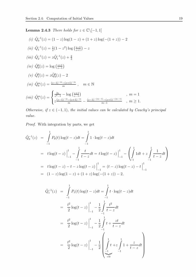
Lemma 2.4.3 There holds for z ∈ C\[−1, 1]
(i) Q−10 (z) = (1− z) log(1− z) + (1 + z) log(−(1 + z))− 2
(ii) Q−11 (z) = 1
2(1− z2) log
(z−1z+1
)− z
(iii) Q−12 (z) = zQ−1
1 (z) + 23
(iv) Q00(z) = log
(z+1z−1
)
(v) Q01(z) = zQ0
0(z)− 2
(vi) Qm0 (z) =
(z−1)−m−(z+1)−m
m, m ∈ N
(vii) Qm1 (z) =
2zz2−1
− log(z+1z−1
), m = 1
z(z−1)−m−(z+1)−m
m− (z−1)−(m−1)−(z+1)−(m−1)
m−1, m ≥ 1.
Otherwise, if z ∈ (−1, 1), the initial values can be calculated by Cauchy’s principal
value.
Proof. With integration by parts, we get
Q−10 (z) =
1∫
−1
P0(t) log(t− z)dt =
1∫
−1
1 · log(t− z)dt
= t log(t− z)∣∣∣
1
−1−
1∫
−1
t
t− zdt = t log(t− z)
∣∣∣
1
−1−
1∫
−1
1dt+ z
1∫
−1
1
t− zdt
= t log(t− z)− t− z log(t− z)∣∣∣
1
−1= (t− z) log(t− z)− t
∣∣∣
1
−1
= (1− z) log(1− z) + (1 + z) log(−(1 + z))− 2,
Q−11 (z) =
1∫
−1
P1(t) log(t− z)dt =
1∫
−1
t · log(t− z)dt
=t2
2log(t− z)
∣∣∣∣
1
−1
− 1
2
1∫
−1
t2
t− zdt
=t2
2log(t− z)
∣∣∣∣
1
−1
− 1
2
1∫
−1
t +zt
t− zdt
=t2
2log(t− z)
∣∣∣∣
1
−1
− 1
2
1∫
−1
t
︸︷︷︸=0
+z
1∫
−1
1 +z
t− zdt

20 Chapter 2: Three-Term Recurrence Relations
=t2
2log(t− z)− zt
2− z2
2log(t− z)
∣∣∣∣
1
−1
=1
2(t2 − z2) log(t− z)− zt
2
∣∣∣∣
1
−1
=1
2(1− z2) log
(z − 1
z + 1
)
− z
and
Q−12 (z) =
1∫
−1
P2(t) log(t− z)dt =1
2
1∫
−1
(3t2 − 1) log(t− z)dt
=1
2
3
1∫
−1
t2 log(t− z)dt−1∫
−1
log(t− z)dt
=1
2
3
1
3t3log(t− z)
∣∣∣∣
1
−1
− 1
3
1∫
−1
t3
t− zdt
− Q−10 (z)
=1
2
t3log(t− z)∣∣∣
1
−1−
1∫
−1
t3
t− zdt− Q−1
0 (z)
.
We use Lemma 2.4.1 and obtain
Q−12 (z) =
1
2
(
(1− z3) log(1− z) + (1 + z3) log(−(1 + z))− 2z2 − 2
3− Q−1
0 (z)
)
=1
2
(
(1− z3) log(1− z) + (1 + z3) log(−(1 + z))− 2z2 − 2
3
−(1− z) log(1− z)− (1 + z) log(−(1 + z)) + 2)
=1
2
(
(z − z3) log(1− z) + (z3 − z) log(−(1 + z))− 2z2 +4
3
)
= z
(1
2(1− z2) log
(z − 1
z + 1
)
− z
)
+2
3
= zQ−11 (z) +
2
3.
We calculate the initial values of Qmk (z). There holds
Q00(z) =
1∫
−1
1
z − tdt = − log(z − t)
∣∣∣
1
−1
= log
(z + 1
z − 1
)
Qm0 (z) =
1∫
−1
1
(z − t)m+1dt =(z − t)−m
m
∣∣∣∣
1
−1

Section 2.4: Computation of Initial Values 21
=(z − 1)−m − (z + 1)−m
m, m ∈ N
Q01(z) =
1∫
−1
t
z − tdt = −z log(z − t)− t
∣∣∣
1
−1
= z log
(z + 1
z − 1
)
− 2 = zQ00(z)− 2
Qm1 (z) =
1∫
−1
t
(z − t)m+1dt =
1∫
−1
z − (z − t)
(z − t)m+1 dt
= z
1∫
−1
1
(z − t)m+1dt−1∫
−1
1
(z − t)mdt
= zQm0 (z)− Qm−1
0 (z) , m ∈ N.
=
2zz2−1
− log(z+1z−1
), m = 1
z(z−1)−m−(z+1)−m
m− (z−1)−(m−1)−(z+1)−(m−1)
m−1, m ≥ 1
2.4.2 Initial Values of Nk(t)
The next lemma contains the first values of Nk(t).
Lemma 2.4.4 There holds
(i) N1(t) =12(1− t)
(ii) N2(t) =12(1 + t)
(iii) N3(t) =12(t2 − 1)
(iv) N4(t) =12(t3 − t).
Proof. ad (i), ad (ii) Nothing to show.
ad (iii), ad (iv) We use property (i) of Lemma 2.1.1 to rewrite N3(t) and N4(t). We
obtain
N3(t) =
t∫
−1
P1(ξ)dξ =1
3(P2(t)− P0(t))
=1
3
(3
2t2 − 1
2− 1
)
=1
2(t2 − 1)

22 Chapter 2: Three-Term Recurrence Relations
and
N4(t) =
t∫
−1
P2(ξ)dξ =1
5(P3(t)− P1(t))
=1
5
(5
2t3 − 3
2t− t
)
=1
2(t3 − t).
2.4.3 Initial Values of Rm
k(z)
The next lemma contains the initial values of Rmk (z).
Lemma 2.4.5 There holds for z ∈ C\[−1, 1]
(i) R−11 (z) =
(34+ 1
2z − 1
4z2)log(−1 − z) +
(14− 1
2z + 1
4z2)log(1− z) + 1
2z − 1
(ii) R−12 (z) =
(14+ 1
2z + 1
4z2)log(−1− z) +
(34− 1
2z + 1
4z2)log(1− z)− 1
2z − 1
(iii) R−13 (z) =
(−1
3− 1
2z + 1
6z3)log(−1− z)+
(−1
3+ 1
2z − 1
6z3)log(1− z)− 1
3z3+ 8
9
(iv) R−14 (z) = −1
8(z4 − 2z2 + 1) log
(z−1z+1
)− 1
4z3 + 5
12z
(v) Rm1 (z) =
13(Qm
0 (z)− Qm1 (z))
(vi) Rm2 (z) =
13(Qm
0 (z) + Qm1 (z))
(vii) Rm3 (z) =
13(Qm
2 (z)− Qm0 (z))
(viii) Rm4 (z) =
15(Qm
3 (z)− Qm1 (z)).
Otherwise, if z ∈ (−1, 1), the initial values can be calculated by Cauchy’s principal
value.
Proof. We calculate the initial values by using lemma (2.4.1). There holds
R−11 (z) =
1∫
−1
N1(t) log(t− z)dt =1
2
1∫
−1
(1− t) log(t− z)dt
=1
2
1∫
−1
log(t− z)dt−1∫
−1
t log(t− z)dt
=
(3
4+
1
2z − 1
4z2)
log(−1− z) +
(1
4− 1
2z +
1
4z2)
log(1− z) +1
2z − 1,

Section 2.4: Computation of Initial Values 23
R−12 (z) =
1∫
−1
N2(t) log(t− z)dt =1
2
1∫
−1
(1 + t) log(t− z)dt
=1
2
1∫
−1
log(t− z)dt+
1∫
−1
t log(t− z)dt
=
(1
4+
1
2z +
1
4z2)
log(−1− z) +
(3
4− 1
2z +
1
4z2)
log(1− z)− 1
2z − 1,
R−13 (z) =
1∫
−1
N3(t) log(t− z)dt =1
2
1∫
−1
(t2 − 1) log(t− z)dt
=1
2
1∫
−1
t2 log(t− z)dt−1∫
−1
log(t− z)dt
=
(
−1
3− 1
2z +
1
6z3)
log(−1− z) +
(
−1
3+
1
2z − 1
6z3)
log(1− z)− 1
3z3 +
8
9
and
R−14 (z) =
1∫
−1
N4(t) log(t− z)dt =1
2
1∫
−1
(t3 − t) log(t− z)dt
=1
2
1∫
−1
t3 log(t− z)dt−1∫
−1
t log(t− z)dt
= −1
8(z4 − 2z2 + 1) log
(z − 1
z + 1
)
+5
12z − 1
4z3.
We use the relation of Lemma 2.3.6 and obtain the remaining values.
Remark 2.4.6 There holds for z ∈ C\[−1, 1]
(i) R01(z) =
1−z2
log(z+1z−1
)+ 1
(ii) R02(z) =
1+z2
log(z+1z−1
)− 1
(iii) R03(z) =
z2−12
log(z+1z−1
)− z
(iv) R04(z) =
z3−z2
log(z+1z−1
)− z2 + 2
3
(v) R11(z) =
12log(z+1z−1
)− 1
z+1
(vi) R12(z) = −1
2log(z+1z−1
)+ 1
z−1
(vii) R13(z) = −z log
(z+1z−1
)+ 2
(viii) R14(z) =
12(1− 3z2) log
(z+1z−1
)+ 3z.
Otherwise, if z ∈ (−1, 1), the initial values can be calculated by Cauchy’s principal
value.

24 Chapter 2: Three-Term Recurrence Relations

Chapter 3
Stable Numerical Calculation of
Minimal Solutions
We introduced several three-term recurrence relations and their related initial values
in the previous chapter, but we don’t discuss the stability of evaluating them. Hence,
we take a look on computational aspects and notice, that the forward evaluation is
not stable outside the real interval [−1, 1], but the area, in which the relative error
is smaller than a given tolerance, is an ellipse on the complex plane around the
real interval [−1, 1]. Two algorithms are introduced, which steady the calculation
outside [−1, 1]. We give the implementation of all algorithms in Matlab. First
of all, we motivate the idea of a minimal and dominant solution of a three-term
recurrence relation with the following example. In fact, there exists other types of
solutions, too.
Example 3.0.1 A unified three-term recurrence relation
xk+1 = axk + bxk−1 , a, b 6= 0, b 6= −a2
4
can be written as
(
xk+1
xk
)
= A
(
xk
xk−1
)
with A =
(
a b
1 0
)
.
The eigenvalues are
λ1 =a+
√a2 + 4b
2and λ2 =
a−√a2 + 4b
2.
The eigenpairs are denoted by (v1, λ1), (v2, λ2). We can choose the initial values
(
x1
x0
)
= µ1v1 + µ2v2 , µ1, µ2 6= 0
as a linear combination of eigenvectors, because the assumptions of a and b guarantee
rang(A) = 2. Based on Theorem 2.1 and Theorem 2.2 of [5] there holds
|λ2| < 1 < |λ1|.

26 Chapter 3: Stable Numerical Calculation of Minimal Solutions
For k = 1, we get
(
x2
x1
)
= A
(
x1
x0
)
= µ1Av1 + µ2Av2
= µ1λ1v1 + µ2λ2v2.
This leads to(
xk+1
xk
)
= µ1λk1v1 + µ2λ
k2v2.
For k → ∞, there holds
λk1v1 → +∞ and λk
2v2 → 0.
Due to this fact, a three-term recurrence relation can be represented as a linear
combination of a dominat solution, because it converges to infinity, and a minimal
solution, because it converges to zero, if they exist.
We define the minimal and dominant solution of a three-term recurrence relation,
without making constraint for the recurrence matrix.
Definition 3.0.2 (Minimal and dominant solution) A solution uk(z) of a
three-term recurrence relation is said to be minimal, if there exists a linearly in-
dependent solution vk(z) of the same three-term recurrence relation such that
limk→∞
uk(z)
vk(z)= 0, (3.1)
and vk(z) is called dominant solution.
3.1 Forward Evaluation
The forward evaluation is the simpliest and more intuitive way to calculate a solution
of a three-term recurrence relation. We consider the three-term recurrence relations
as in the first chapter
(k − n+ 1)fk+1+s(z) = (2k + 1)zfk+s(z)− (k + n)fk−1+s(z) , k ∈ N, s, n ∈ Z
and a vector f ∈ Cj with the related initial values.
3.1.1 Implementation in Matlab
Section 3.1: Forward Evaluation 27
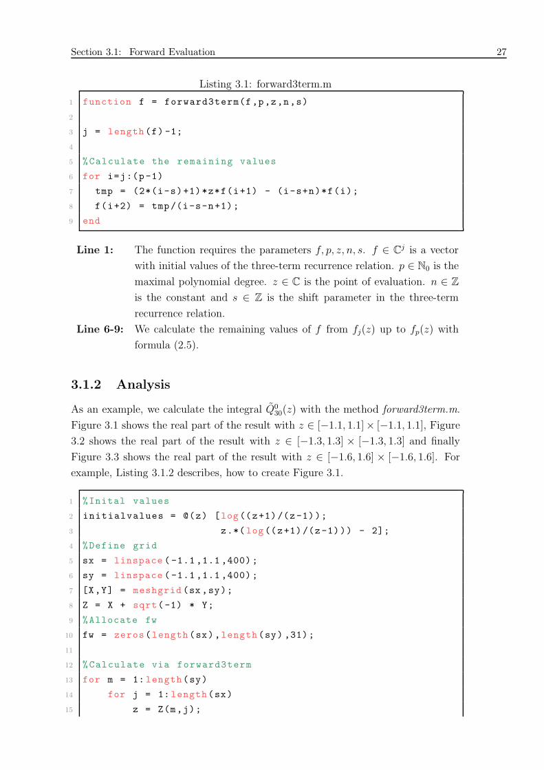
Listing 3.1: forward3term.m
1 function f = forward3term(f,p,z,n,s)
2
3 j = length(f) -1;
4
5 %Calculate the remaining values
6 for i=j:(p-1)
7 tmp = (2*(i-s)+1)*z*f(i+1) - (i-s+n)*f(i);
8 f(i+2) = tmp/(i-s-n+1);
9 end
Line 1: The function requires the parameters f, p, z, n, s. f ∈ Cj is a vector
with initial values of the three-term recurrence relation. p ∈ N0 is the
maximal polynomial degree. z ∈ C is the point of evaluation. n ∈ Z
is the constant and s ∈ Z is the shift parameter in the three-term
recurrence relation.
Line 6-9: We calculate the remaining values of f from fj(z) up to fp(z) with
formula (2.5).
3.1.2 Analysis
As an example, we calculate the integral Q030(z) with the method forward3term.m.
Figure 3.1 shows the real part of the result with z ∈ [−1.1, 1.1]× [−1.1, 1.1], Figure
3.2 shows the real part of the result with z ∈ [−1.3, 1.3] × [−1.3, 1.3] and finally
Figure 3.3 shows the real part of the result with z ∈ [−1.6, 1.6] × [−1.6, 1.6]. For
example, Listing 3.1.2 describes, how to create Figure 3.1.
1 %Inital values
2 initialvalues = @(z) [log((z+1)/(z-1));
3 z.*(log((z+1)/(z-1))) - 2];
4 %Define grid
5 sx = linspace ( -1.1 ,1.1 ,400);
6 sy = linspace ( -1.1 ,1.1 ,400);
7 [X,Y] = meshgrid (sx,sy);
8 Z = X + sqrt(-1) * Y;
9 %Allocate fw
10 fw = zeros(length(sx),length(sy) ,31);
11
12 %Calculate via forward3term
13 for m = 1: length(sy)
14 for j = 1:length(sx)
15 z = Z(m,j);

28 Chapter 3: Stable Numerical Calculation of Minimal Solutions
16 f = initialvalues(z);
17 fw(m,j,1:end) = forward3term(f,30,z,0,0);
18 end
19 end
20
21 %Surf result
22 surf(X,Y,real(fw(:,:,end)))
23 shading flat
24 axis tight
We recognize, that in general the forward evaluation is numerically unstable comput-
ing a minimal solution. In fact, three-term recurrence relations have a bad condition
with respect to minimal solutions. There is no problem calculating a dominant so-
lution. That is the reason, why we discuss alternative algorithms to calculate a
minimal solution of a three-term recurrence relation. In Figure 3.3, you may detect,
that the area, in which the relative error of the forward evaluation is small, is located
around an ellipse relative to the real interval [−1, 1]. The main object will be the
determination of the ellipse parameters to gain a border, which divides the complex
plane into two areas. Inside the ellipse, we can calculate the minimal solution via
forward evaluation and outside, we use an alternative algorithm.
Figure 3.1: Real part of the result of forward evaluation of Q030(z) on [−1.1, 1.1]2.
3.2 Miller’s Backward Algorithm
To get a better condition for calculating a minimal solution of a three-term recur-
rence relation, Miller suggests to compute the values backward by using the property

Section 3.2: Miller’s Backward Algorithm 29
Figure 3.2: Real part of the result of forward evaluation of Q030(z) on [−1.3, 1.3]2.
Figure 3.3: Real part of the result of forward evaluation of Q030(z) on [−1.6, 1.6]2.
of a minimal solutions, that they converge to zero. We consider the three-term re-
currence relations as in the first chapter
(k − n+ 1)fk+1+s(z) = (2k + 1)zfk+s(z)− (k + n)fk−1+s(z) , k ∈ N, s, n ∈ Z
and a vector f ∈ Cj with the related initial values. We rewrite the last equation
and obtain the formula
fk−1+s(z) =2k + 1
k + nzfk+s(z)−
k − n+ 1
k + nfk+1+s(z) , k ∈ N, s, n ∈ Z (3.2)
to calculate the values backward. We choose an arbitrary start index ν, set fν+1(z) =
0 and fν(z) = 1 and calculate the remaining values of fk(z) down to fp(z). We repeat
this procedure until the relative error between the previous and the current values
of fp+1(z) and fp(z) are smaller than a tolerance or ν is larger than an upper bound
νmax.

30 Chapter 3: Stable Numerical Calculation of Minimal Solutions
3.2.1 Implementation in Matlab
Listing 3.2: backward3term.m
1 function [f,nu] = backward3term(f,p,z,n,s)
2
3 %Preperations
4 tol = 1e-14;
5 told = [realmax ;1];
6 %Set nu arbitrary (nu > p )
7 nu = p+2;
8 nu_max = 5000;
9 %Set initial values
10 t = [1;0];
11
12 while nu < nu_max
13 %Save only the last two entries
14 for i = nu:-1:p
15 t= [((2*(i-s)+1)*z*t(1) -((i-s)-n+1)*t(2))/((i-s)+n);
16 t(1)];
17 t = t./norm(t);
18 end
19 t = t./t(2);
20 %Check , if t is a good approximation
21 if sum(abs(told -t)<tol*abs(t)) == 2
22 break;
23 end
24 told = t;
25 nu = nu + 1;
26 end
27
28 j = length(f) -1;
29 tmp = f(end);
30 f(p:p+1) = t;
31 %Calculate the remaining values
32 for i=p-1:-1:j+1
33 f(i)=((2*(i-s)+1)*z*f(i+1) -((i-s)-n+1)*f(i+2))/((i-s)+n);
34 end
35 %Multiply with tmp/f(j+1), because f(j+1) was overwritten
36 f(j+1:end) = f(j+1:end) * tmp/f(j+1);

Section 3.3: Gautschi’s Continued Fraction Algorithm 31
Line 1: The function requires the parameters f, p, z, n, s. f ∈ Cj is a
vector with initial values of the three-term recurrence relation.
p ∈ N0 is the maximal polynomial degree. z ∈ C is the point
of evaluation. n ∈ Z is the constant and s ∈ Z is the shift
parameter in the three-term recurrence relation.
Line 4-10: We set the tolerance tol = 1e − 14 and ν = p + 2 arbitrary.
We define an upper border for ν to avoid an endless loop. In
Line 10 we set the initial values such that t(1) = fν(z) = 1 and
t(2) = fν+1(z) = 0
Line 12, 21-23: The breaking conditions for the while-loop. If ν become larger
than an upper bound or the relative error between the previous
and current values of t(1) = fp(z) and t(2) = fp−1(z) is smaller
than a tolerance tol, we don’t continue calculating the values
for fν−1(z) . . . fp−1(z) again.
Line 14-18: We calculate the values fν−1(z) down to fp(z) with formula
(3.2). We have to save only the last two entries, because af-
ter the for- loop we only compare t with told.
Line 24-25: If t doesn’t satisfy the break condition in Line 21, we set told = t,
increase ν = ν + 1 and repeat the procedure from Line 12-26.
Line 29: We store the last initial value tmp = fj−1(z), because we over-
write it.
Line 32-34: We calculate the values fp−2(z) down to fj−1(z) with formula
(3.2).
Line 36: We scale the computed values of f with tmp
fj−1(z)to get the correct
values.
3.3 Gautschi’s Continued Fraction Algorithm
We consider a the three-term recurrence relations as in the first chapter
(k − n+ 1)fk+1+s(z) = (2k + 1)zfk+s(z)− (k + n)fk−1+s(z) , k ∈ N, s, n ∈ Z
and a vector f ∈ Cj with the related initial values. Gautschi’s continued fraction
algorithm is based on the theory of continued fractions and their convergence. For
further information see [6]. In Lemma 2.2.2 we proved a transformation formula
for fk(z) in order that the leading coefficients are equal to one, because Gautschi’s
continued fraction algorithm requires a system of polynomials of this type. While
computing fk(z), instead of fk(z), we modify Gautschi’s continued fraction algo-
rithm.

32 Chapter 3: Stable Numerical Calculation of Minimal Solutions
3.3.1 Implementation in Matlab
Listing 3.3: gautschi.m
1 function [f, nu] = gautschi(f,p,z,n,s)
2
3 fold = 1;
4 fn = 0;
5 tol = 1e-14;
6 nu = p+1;
7 nmax = 1e8;
8 j = length(f) -1;
9
10
11 while abs(fold -fn) > tol*abs(fold) && nu < nmax
12
13 %Calculate vector r
14 r(nu+1) = 1;
15 for m = nu:-1:j
16 bm = ((m-s)+n)*((m-s)-n)/((2*(m-s) -1)*(2*(m-s)+1));
17 r(m) = bm / (z - r(m+1));
18 end
19
20 %Store the last initial value
21 tmp = f(j+1);
22 f(j+1) = 1;
23 %First factor is based on transformation formula
24 for m = j+1:p
25 f(m+1) = (2*(m-s) -1)/((m-s)-n) * r(m)*f(m);
26 end
27 %Scale the computed value
28 f(j+1) = tmp;
29 f(j+2:end) = tmp*f(j+2:end);
30
31 fold = fn;
32 fn = f(p+1);
33 nu = nu + 1;
34 end

Section 3.4: Estimate of ν as Against Adaptive Determination 33
Line 1: The function requires the parameters f, p, z, n, s. f ∈ Cj is a vector
with initial values of the three-term recurrence relation. p ∈ N0 is
the maximal polynomial degree. z ∈ C is the point of evaluation.
n ∈ Z is the constant and s ∈ Z is the shift parameter in the three-
term recurrence relation.
Line 5-6: We set the tolerance tol = 10−14 and ν = p+ 1 arbitrary.
Line 11: The break condition of the while-loop. If ν become larger than an
upper bound or the relative error between the previous and current
values of fp(z) is smaller than a tolerance tol, we don’t continue
calculating the values for fj(z) . . . fp(z) again.
Line 14-18: The calculation of vector r as Gautschi suggests in his paper [6] (Eq
5.1).
rm−1(z) =bm
z − am − rm, m = ν − 1, . . . , 1
with rν = 0. Note, that in our case am = 0 for all m ∈ N. Lemma
2.2.2 supplies a formula for
bm =(m− n)(m+ n)
(2m− 1)(2m+ 1),
without an index shift. In Line 16, we insert the shift.
Line 20-21: We store the last initial value in tmp, because we compute the re-
maining values respectively to fj−1(z), which is set to 1.
Line 24-27: The formula to calculate the minimal solution is given by [6] (Eq
5.1). In fact, we don’t expect, that the system of fk(z) has the
leading coefficient equal to one, we modify the formula. Lemma
2.2.2 supplies
fm(z) =2m− 1
m− n· rm−1 · fm−1(z).
In Line 25, we insert the shift again.
Line 28-29: Due to the fact, that we set fj−1(z) = 1, we have to scale the
computed values with tmp.
3.4 Estimate of ν as Against Adaptive Determi-
nation
We want to compare Gautschi’s continued fraction algorithm and Miller’s backward
algorithm with respect to to the maximal ν of each point to get a exact solution.
In fact, we have two algorithm to calculate a minimal solution, which are numerical
stable on the complete complex plane. But close to the real interval [−1, 1], we need

34 Chapter 3: Stable Numerical Calculation of Minimal Solutions
many iterations to get an exact solution, in other words ν increases very fast, when
z ∈ C is close to [−1, 1]. Figure 3.4 shows the maximal ν calculating Q0k(z) for
k = 0 . . . 100 (left: via Miller’s backward algorithm, right: via Gautschi’s continued
fraction algorithm) - more precisely, the figure shows the maximal ν for each point,
whose the break condition of the while-loop (in backward3term.m Line 12 and in
gautschi.m Line 11) is satisfied. This figure illustrates the biggest disadvantage
of both algorithms - the low convergence close to the real interval [−1, 1]. It is
desirable to have a stable algorithm with a high convergence. We can optimize
500
500
1000
1000
15001500
20002000
2500
0 0.1 0.2 0.3 0.4 0.5 0.6 0.7 0.8 0.9
0.01
0.015
0.02
0.025
0.03
500
500
1000
1000
1500
1500
20002000
25002500
3000
0 0.1 0.2 0.3 0.4 0.5 0.6 0.7 0.8 0.9
0.01
0.015
0.02
0.025
0.03
0.035
0.04
Figure 3.4: Maximal ν for each point. Left: Calculated via backward3term. Right:
Calculated via gautschi.m.
Gautschi’s continued fraction algorithm estimating a useful initial value of the index
ν to prevent the while-loop in Line 11.
Let be uk(z) the minimal solution and pk(z) the dominant solution with p−1(z) = 0
and p0(z) = 1 of the three-term recurrence relation
(k − n+ 1)fk+1+s(z) = (2k + 1)zfk+s(z)− (k + n)fk−1+s(z) , k ∈ N, s, n ∈ Z.
It holds uk(z)pk(z)
→ 0 for k → ∞ and for sufficiently large N , the relative error can be
approximated by
max1≤n≤N
|ǫ(ν)n | = |ǫ(ν)N | =∣∣∣∣
uν(z)
pν(z)· pN(z)uN(z)
∣∣∣∣,
see also [5] (3.18). An asymptotic formula for uk(z)pk(z)
is given in the appendix of [3]
(Eq. A.1). Thus we have
uν(z)
pν(z)· pN(z)uN(z)
∼(
1
z +√z2 − 1
)2(ν−N)
.
Given a tolerance ǫ > 0, we want to determine ν, such that the relative error is
smaller than ǫ, therefore
ǫ!=
(1
z +√z2 − 1
)2(ν−N)

Section 3.5: Error Analysis and Ellipse Parameters 35
must apply. This is equivalent to
log (ǫ) = log
((1
z +√z2 − 1
)2(ν−N))
= 2(ν −N) log
(1
z +√z2 − 1
)
= 2(ν −N)(
log (1)− log (z +√
z2 − 1))
= −2(ν −N) log (z +√
z2 − 1)
We multiply the last equation with −1, divide by log (z +√z2 − 1) and obtain
2(ν −N) =log(1ǫ
)
log (z +√z2 − 1)
ν = N +log(1ǫ
)
2 log (z +√z2 − 1)
.
Thus, to have a precision ǫ for un(z), we have to choose
ν ≥ n+log(1ǫ
)
2 log |z +√z2 − 1|
. (3.3)
3.5 Error Analysis and Ellipse Parameters
In order to choose a favorite algorithm, we make an error analysis with Miller’s
backward algorithm (MBA) and Gautschi’s continued fraction algorithm (GCFA).
We fix two points in C - one close to the singularity and one in the far field - and
compare the exact solution, which is calculated by Maple, with the results of both
algorithms. Afterwards, we want to assign the ellipse parameter by observing the
relative error between the forward evaluation and Gautschi’s continued fraction al-
gorithm. We noted previously, that the forward evaluation has a small relative error
with respect to the exact solution inside an ellipse. Consequently, we want to deter-
mine the ellipse parameter to have a tool, which allows us to decide, when we have to
switch between the forward evaluation and an alternative algorithm. Therefore, we
avoid the problem of the low convergence close to the real interval [−1, 1], because
there, we use the forward evaluation.
Table 3.4 contains the absolute error between both algorithms with respect to the
exact solution, which is evaluated close to the singularity, thus we chose z = 1+0.1i.
Table 3.5 contains the absolute error between both algorithms with respect to to
the exact solution, which is evaluated in the far field, therefore we chose z = 2+ 3i.
We note, that machine precision is reached. That is the reason, why there are a few
irregularities, especially for the initial values.

36 Chapter 3: Stable Numerical Calculation of Minimal Solutions
Figure 3.5: An ellipse.
Furthermore we investigate the relative error of Q0k(z) calculating via Miller’s back-
ward algorithm and Gautschi’s continued fraction algorithm respectively to the exact
solution at z = 1 + 0.1i, which is calculated by Maple, as depicted in Figure 3.6.
Next, we want to assign the ellipse parameter looking at the relative error between
the forward evaluation and Gautschi’s continued fraction algorithm. We give a short
summary of relevant ellipse parameter and properties.
Figure 3.5 shows an ellipse with the parameters
a,b - length of the half-axis,
F1,F2 - foci of the ellipse.
In our case, the foci of the ellipse are F1 = −1 and F2 = 1. Two formulas of the
ellipse parameters of a point z ∈ C are given by
a =1
2(|z + 1|+ |z − 1|),
b =
√
(|z + 1|+ |z − 1|)24
− 1.
Now, we investigate the relative error between the forward evaluation and Gautschi’s
continued fraction algorithm. We determine for each polynomial degree the
minimal b such that the relative error is greater than a given tolerance tol ∈{10−8, 10−9, 10−10, 10−11, 10−12, 10−13}. As an example Figure 3.7 shows the results
of calculation theses ellipse parameters for Q0k(z) for k = 0 . . . 1000 and Figure 3.7
shows the results of calculation theses ellipse parameters for R0k(z) for k = 1 . . . 1000.
We find a lower bound with the function
b(k) = min
(
1,4.5
(k + 1)1.17
)
(3.4)

Section 3.5: Error Analysis and Ellipse Parameters 37
101
102
103
10−15
10−14
Polynomial degree k
Rel
ativ
e er
ror
resp
ectiv
ely
to th
e ex
act s
olut
ion
err(backward)err(gautschi)
Figure 3.6: Relative error at z = 1 + 0.1i.
z = 1 + 0.1i MBA GCFA
Q00(z) 0.0000 0.0000
Q01(z) 0.0000 0.0000
Q02(z) 0.1110e-15 0.1110e-15
Q03(z) 0.1110e-15 0.2220e-15
Q04(z) 0.2776e-15 0.1110e-15
Q05(z) 0.4996e-15 0.0555e-15
Q06(z) 0.4163e-15 0.2776e-15
Q07(z) 0.0139e-15 0.7494e-15
z = 1 + 0.1i MBA GCFA
Q10(z) 0.0000 0.0000
Q11(z) 0.0000 0.0000
Q12(z) 0.0089e-13 0.0001e-13
Q13(z) 0.0089e-13 0.0003e-13
Q14(z) 0.0266e-13 0.0089e-13
Q15(z) 0.0533e-13 0.0222e-13
Q16(z) 0.0400e-13 0.0577e-13
Q17(z) 0.0266e-13 0.1243e-13
z = 1 + 0.1i MBA GCFA
R01(z) 0.0000 0.0000
R02(z) 0.0000 0.0000
R03(z) 0.0000 0.0000
R04(z) 0.0278e-15 0.0833e-15
R05(z) 0.0971e-15 0.0416e-15
R06(z) 0.1735e-15 0.1110e-15
R07(z) 0.1665e-15 0.1388e-15
z = 1 + 0.1i MBA GCFA
R11(z) 0.0000 0.0000
R12(z) 0.0000 0.0000
R13(z) 0.0000 0.0000
R14(z) 0.0444e-14 0.0333e-14
R15(z) 0.1332e-14 0.0222e-14
R16(z) 0.1277e-14 0.1110e-14
R17(z) 0.0312e-14 0.1887e-14
Tab. 3.4: Absolute error of MBA and GCFA for z = 1 + 0.1i.

38 Chapter 3: Stable Numerical Calculation of Minimal Solutions
z = 2 + 3i MBA GCFA
Q00(z) 0.0000 0.0000
Q01(z) 0.8327e-16 0.8327e-16
Q02(z) 0.0781e-16 0.0781e-16
Q03(z) 0.0108e-16 0.0108e-16
Q04(z) 0.0015e-16 0.0014e-16
Q05(z) 0.0002e-16 0.0001e-16
Q06(z) 0.0000e-16 0.0000e-16
Q07(z) 0.0000e-16 0.0000e-16
z = 2 + 3i MBA GCFA
Q10(z) 0.0000 0.0000
Q11(z) 0.0000 0.0000
Q12(z) 0.0434e-16 0.0607e-16
Q13(z) 0.0087e-16 0.0065e-16
Q14(z) 0.0012e-16 0.0012e-16
Q15(z) 0.0002e-16 0.0002e-16
Q16(z) 0.0000e-16 0.0000e-16
Q17(z) 0.0000e-16 0.0000e-16
z = 2 + 3i MBA GCFA
R01(z) 0.0000 0.0000
R02(z) 0.0000 0.0000
R03(z) 0.0000 0.0000
R04(z) 0.1285e-14 0.1285e-14
R05(z) 0.0101e-14 0.0101e-14
R06(z) 0.0009e-14 0.0009e-14
R07(z) 0.0001e-14 0.0001e-14
z = 2 + 3i MBA GCFA
R11(z) 0.0000 0.0000
R12(z) 0.0000 0.0000
R13(z) 0.0083e-14 0.0083e-14
R14(z) 0.1343e-14 0.1344e-14
R15(z) 0.0158e-14 0.0159e-14
R16(z) 0.0019e-14 0.0019e-14
R17(z) 0.0002e-14 0.0002e-14
Tab. 3.5: Absolute error of MBA and GCFA for z = 2 + 3i.
whereas k is the polynomial degree. In fact, we gain a border, which divides the
complex plane into two area. Inside the ellipse with the parameters a and b, we use
the forward evaluation and outside, we use Gautschi’s continued fraction algorithm.
Let be z = u+ iv, then
Calculation at z
via forward evaluation , if a2
u2 +b2
v2< 1
via Gautschi’s continued fraction algorithm , else.
The reasons, why we choose Gautschi’s continued fraction algorithm, are the pre-
cision and the overflow of Miller’s backward algorithm. Numerical experiments
showed, that for p ≫ 1, overflow occurs calculating the minimal solution with
Miller’s backward algorithm.

Section 3.5: Error Analysis and Ellipse Parameters 39
100
101
102
10310
−3
10−2
10−1
100
101
Degree k
Elli
pse
para
met
er b
tol = 1e−8tol = 1e−9tol = 1e−10tol = 1e−11tol = 1e−12tol = 1e−13b(k)
Figure 3.7: Result of calculating the ellipse parameter b for Q0k(z).
100
101
102
10310
−3
10−2
10−1
100
101
Degree k
Elli
pse
para
met
er b
tol = 1e−8tol = 1e−9tol = 1e−10tol = 1e−11tol = 1e−12tol = 1e−13b(k)
Figure 3.8: Result of calculating the ellipse parameter b for R0k(z).

40 Chapter 3: Stable Numerical Calculation of Minimal Solutions

Chapter 4
C-Library ’liblegfct.c’
We want to give an detailed description of the C-Library ’liblegfct.c’, which is found
in the folder ’libbem c’. We use the results of the previous chapter to create a
library, which contains functions calculating minimal solutions numerically stable
and deciding autonomously, which algorithm should be used. The functions exists
as Matlab files as well in the folder ’libbem mat’. We prefer to calculate the
integrals with the C functions, because we reach more performance parallelizing the
computation e.g. via OpenMP or via Nvidia Cuda. Due to this fact, a interface
between Matlab an C is required. In [2] a Mex-interface is introduced, which uses
OpenMP. Instead of explaining the Mex interface, we limit the explanation to the
C-Library. In the end of this chapter, we describe testing the routines in Matlab.
Recall the definitions
Q−1k (z) :=
1∫
−1
Pk(t) log(t− z)dt , k ∈ N0,
Qmk (z) :=
1∫
−1
Pk(t)
(z − t)m+1dt , k,m ∈ N0,
R−1k (z) :=
1∫
−1
Nk(t) log(t− z)dt , k ∈ N,
Rmk (z) :=
1∫
−1
Nk(t)
(z − t)m+1dt , k ∈ N, m ∈ N0.
The C-Library ’liblegfct.c’ includes the following functions:
qtm1 Calculates the integrals Q−1k (z) for one point z ∈ C and k = 0 . . . p.
qt0 Calculates the integrals Q0k(z) for one point z ∈ C and k = 0 . . . p.
qt1 Calculates the integrals Q1k(z) for one point z ∈ C and k = 0 . . . p.
qtn Calculates the integrals Qmk (z) for one point z ∈ C, m = 0 . . . n and
k = 0 . . . p.
q0 Calculates the integrals Q0k(z) for one point z ∈ C and k = 0 . . . p.
q1 Calculates the integrals Q1k(z) for one point z ∈ C and k = 0 . . . p.
qn Calculates the integrals Qmk (z) for one point z ∈ C, m = 0 . . . n and
k = 0 . . . p.

42 Chapter 4: C-Library ’liblegfct.c’
r0 Calculates the integrals R0k(z) for one point z ∈ C and k = 1 . . . p.
r1 Calculates the integrals R1k(z) for one point z ∈ C and k = 1 . . . p.
4.1 The Function qtm1
We give a detailed explanation of qtm1. The functions qt0, qt1, r0 and r1 work
similar. We only adjust the three-term recurrence relations and the related initial
values. The function
void qtm1( fcomplex const z, int const p, double const fac, double *rretmp,
double *rimtmp, double *Vre, double *Vim)
calculates the integrals fac · Q−1k (z) for k = 0 . . . p. The parameters are
fcomplex const z z is the point of evaluation. fcomplex is a struct, which
defines complex numbers (See ’complex.h’).
int const p p is the maximal polynomial degree.
double const fac fac is a factor, which makes the calculation more flexible.
Special cases maybe require a multiplicative factor.
double *rretmp rretmp is a pointer to an array, which is used by Gautschi’s
continued fraction algorithm. The array contains the real
part of the vector r, see Listing 3.3 Line 14-18.
double *rimtmp rimtmp is a pointer to an array, which is used by Gautschi’s
continued fraction algorithm. The array contains the imagi-
nary part of the vector r, see Listing 3.3 Line 14-18.
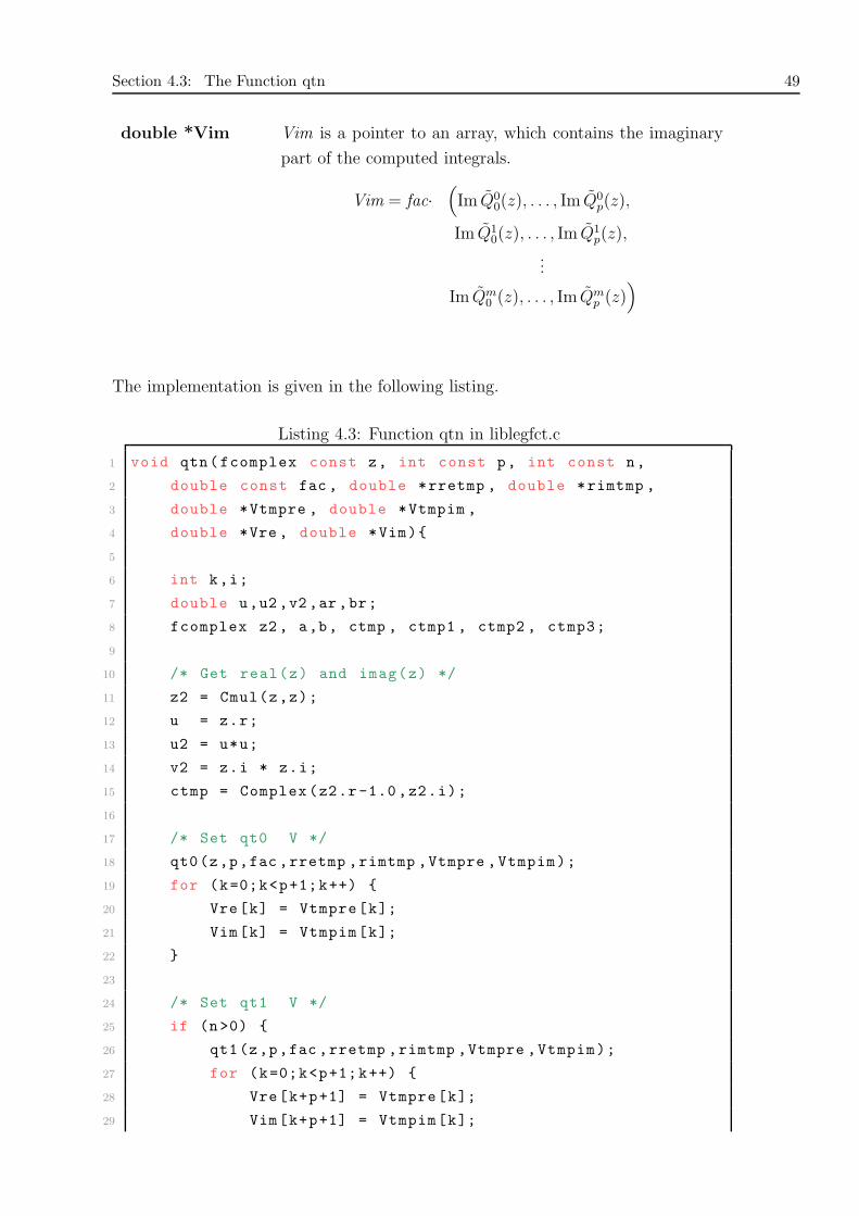
double *Vre Vre is a pointer to an array, which contains the real part of
the computed integrals.
Vre = fac ·(
Re Q−10 (z),Re Q−1
1 (z), . . . ,Re Q−1p (z)
)
double *Vim Vim is a pointer to an array, which contains the imaginary
part of the computed integrals.
Vim = fac ·(
Im Q−10 (z), Im Q−1
1 (z), . . . , Im Q−1p (z)
)
The implementation is given in the following listing.
Listing 4.1: Function qtm1 in liblegfct.c
1 void qtm1(fcomplex const z, int const p, double const fac ,
2 double *rretmp , double *rimtmp ,

Section 4.1: The Function qtm1 43
3 double *Vre, double *Vim){
4
5 int j,n,nu;
6 double tmp00 , tmp01;
7 double a1, a2, a3, u, u2, v, v2, b, b2, b1_2 , b2_2;
8 fcomplex z2, ctmp0 , ctmp1 , ctmp2 , ctmp3;
9 double *rre = rretmp;
10 double *rim = rimtmp;
11
12 /* Get real(z) and imag(z)*/
13 u = z.r;
14 v = z.i;
15 u2 = u*u;
16 v2 = v*v;
17
18 /* Set V[0] and V[1]*/
19 /* case: z is complex */
20 if ( v2 > eps ){
21 a1 = atan((1-u)/v);
22 a2 = atan((1+u)/v);
23 b1_2 = (1+u)*(1+u)+v2;
24 b2_2 = (1-u)*(1-u)+v2;
25 a3 = log(b1_2/b2_2)*0.5;
26
27 Vre[0] = 0.5*log(b1_2*b2_2)+u*a3 -2+v*(a1+a2);
28 Vim[0] = a1-a2-u*(a1+a2)+v*a3-pi*v/fabs(v);
29 if(p>0){
30 Vre[1] = 0.5*a3*(u2-v2 -1) + u*v*(a1+a2)-u;
31 Vim[1] = u*v*a3 -0.5*(u2-v2 -1)*(a1+a2)-v;
32 }
33 /* case: z is real , z != +/- 1*/
34 } else if(u2!=1){
35 a1 = fabs(1+u);
36 a2 = fabs(1-u);
37
38 Vre[0] = log(a1*a2)+u*log(a1/a2) -2;
39 Vim[0] = 0;
40 if(p>0){
41 Vre[1] = 0.5*(u2 -1)*log(a1/a2)-u;
42 Vim[1] = 0;
43 }
44 /* case: z is real , z = +/- 1*/

44 Chapter 4: C-Library ’liblegfct.c’
45 } else {
46 Vre[0] = 2*log(2) -2;
47 Vim[0] = 0;
48 if(p>0){
49 Vre[1] = -u;
50 Vim[1] = 0;
51 }
52 }
53
54 /* Multiply with fac*/
55 Vre[0] *= fac;
56 Vim[0] *= fac;
57 if(p>0){
58 Vre[1] *= fac;
59 Vim[1] *= fac;
60 }
61
62 /* Calculate V[2]..V[p]*/
63 if(p>1){
64
65 /* Ellipse parameters */
66 b = MIN(1 ,4.5/pow(p+1.0,1.17));
67 b2 = b*b;
68 a2 = 1.0+b2;
69
70 /* Inside ellipse: calculation via forward eval */
71 if (u2/a2+v2/b2 < 1) {
72 /* Calculate initial values */
73 ctmp0 = Cmul(z,Complex(Vre[1],Vim[1]));
74 Vre[2] = (fac*2.0) /3.0 + ctmp0.r;
75 Vim[2] = 0.0 + ctmp0.i;
76
77 /* Forward recurrence */
78 for(j=2; j<=p-1; j++){
79 tmp00 = (2.0*j+1.0)/(j+2.0);
80 tmp01 = (1.0-j)/(j+2.0);
81 ctmp0.r = tmp00*z.r;
82 ctmp0.i = tmp00*z.i;
83 ctmp1 = Cmul(ctmp0 , Complex(Vre[j],Vim[j]));
84 ctmp2.r = tmp01* Vre[j-1];
85 ctmp2.i = tmp01* Vim[j-1];
86

Section 4.1: The Function qtm1 45
87 Vre[j+1] = ctmp1.r + ctmp2.r;
88 Vim[j+1] = ctmp1.i + ctmp2.i;
89 }
90 /* Outside of ellipse , calculation via Gautschi */
91 } else {
92 /* Assign nu */
93 z2 = Complex(fabs(u),fabs(v));
94 ctmp0 = Csqrt(Cadd(Complex (-1.0,0), Cmul(z2,z2)));
95 tmp00 = 2*log(Cabs(Cadd(z2, ctmp0)));
96 nu = (int) (p+ceil(log(INVTOL)/tmp00));
97
98 /* Catch case of overflow : Allocate more memory */
99 if(nu>MAX_NU){
100 FILE* of = fopen("nu_overflow.txt","w+");
101 fprintf(of, "nu = %d\n", nu);
102 fclose(of);
103 rre = (double*) malloc(nu*sizeof(double));
104 rim = (double*) malloc(nu*sizeof(double));
105 }
106
107 /* Set initial values */
108 rre[nu -1] = 1;
109 rim[nu -1] = 0;
110 /* Calculate vector r */
111 for (n=nu; n>=2; n--){
112 ctmp3 = Csub(z,Complex(rre[n-1],rim[n-1]));
113 tmp00 = (n*n-1.0) /((4*n*n-1.0)*(ctmp3.r*ctmp3.r
114 + ctmp3.i*ctmp3.i));
115 rre[n-2] = tmp00*ctmp3.r;
116 rim[n-2] = -tmp00*ctmp3.i;
117 }
118
119 /* Calculate remaining values of V */
120 for (n=2; n<p+1; n++){
121 ctmp3 = Cmul(Complex(rre[n-2],rim[n-2]),
122 Complex(Vre[n-1],Vim[n-1]));
123 tmp00 = (2*n-1.0)/(n+1.0);
124 Vre[n] = tmp00*ctmp3.r;
125 Vim[n] = tmp00*ctmp3.i;
126 }
127 }/* end else */
128 }/* end if p > 1*/
46 Chapter 4: C-Library ’liblegfct.c’
129 }/* end qtm1 */
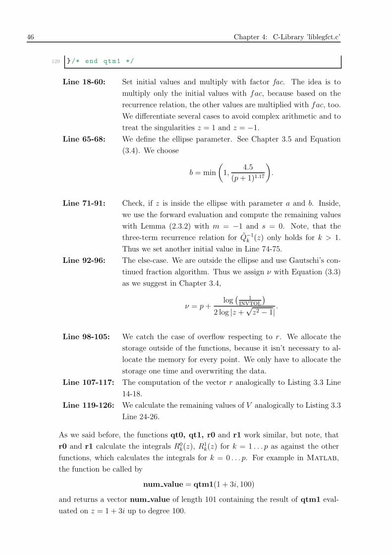
Line 18-60: Set initial values and multiply with factor fac. The idea is to
multiply only the initial values with fac, because based on the
recurrence relation, the other values are multiplied with fac, too.
We differentiate several cases to avoid complex arithmetic and to
treat the singularities z = 1 and z = −1.
Line 65-68: We define the ellipse parameter. See Chapter 3.5 and Equation
(3.4). We choose
b = min
(
1,4.5
(p+ 1)1.17
)
.
Line 71-91: Check, if z is inside the ellipse with parameter a and b. Inside,
we use the forward evaluation and compute the remaining values
with Lemma (2.3.2) with m = −1 and s = 0. Note, that the
three-term recurrence relation for Q−1k (z) only holds for k > 1.
Thus we set another initial value in Line 74-75.
Line 92-96: The else-case. We are outside the ellipse and use Gautschi’s con-
tinued fraction algorithm. Thus we assign ν with Equation (3.3)
as we suggest in Chapter 3.4,
ν = p+log(
1INVTOL
)
2 log |z +√z2 − 1|
.
Line 98-105: We catch the case of overflow respecting to r. We allocate the
storage outside of the functions, because it isn’t necessary to al-
locate the memory for every point. We only have to allocate the
storage one time and overwriting the data.
Line 107-117: The computation of the vector r analogically to Listing 3.3 Line
14-18.
Line 119-126: We calculate the remaining values of V analogically to Listing 3.3
Line 24-26.
As we said before, the functions qt0, qt1, r0 and r1 work similar, but note, that
r0 and r1 calculate the integrals R0k(z), R
1k(z) for k = 1 . . . p as against the other
functions, which calculates the integrals for k = 0 . . . p. For example in Matlab,
the function be called by
num value = qtm1(1 + 3i, 100)
and returns a vector num value of length 101 containing the result of qtm1 eval-
uated on z = 1 + 3i up to degree 100.

Section 4.2: The Function q0 47
4.2 The Function q0
We give a detailed explanation of q0. The function q1 works similar. We use the
relation (i) of Lemma 2.3.1 and the routines qt0 and qt1 to get the values for q0
and q1. The function
void q0( fcomplex const z, int const p, double const fac, double *rretmp,
double *rimtmp, double *Vre, double *Vim)
calculates the integrals fac ·Q0k(z) for k = 0 . . . p. The parameters fcomplex const
z, int const p and double const fac are similar to qtm1. The other parameters
are
double *rretmp rretmp is a pointer to an array, which is used by qt0.
double *rimtmp rimtmp is a pointer to an array, which is used by qt0.
double *Vre Vre is a pointer to an array, which contains the real part
of the computed integrals.
Vre = fac ·(ReQ0
0(z),ReQ01(z), . . . ,ReQ
0p(z)
)
double *Vim Vim is a pointer to an array, which contains the imaginary
part of the computed integrals.
Vim = fac ·(ImQ0
0(z), ImQ01(z), . . . , ImQ0
p(z))
Listing 4.2: Function q0 in liblegfct.c
1 void q0(fcomplex const z, int const p, double const fac ,
2 double *rretmp , double *rimtmp ,
3 double *Vre , double *Vim){
4
5 int k;
6 /* Get qt0 */
7 qt0(z,p,fac ,rretmp ,rimtmp ,Vre ,Vim);
8
9 /* Multiply V with 0.5 and fac */
10 for (k=0;k<p+1;k++) {
11 Vre[k] = fac *0.5*Vre[k];
12 Vim[k] = fac *0.5*Vim[k];
13 }
14 }

48 Chapter 4: C-Library ’liblegfct.c’
Line 7: Calculate the values with qt0 and store them in Vre and Vim.
Line 10-13: We use the relation
Q0k(z) =
0!
2Q0
k
and override the values in Vre and Vim.
4.3 The Function qtn
We give a detailed explanation of qtn. The function qn works similar. In Chapter
2.3.1 we proved a three-term recurrence relation for Qmk (z) over m. As against the
functions, we treated before, the method
void qtn( fcomplex const z, int const p, int const n, double const fac,
double *rretmp, double *rimtmp, double *Vtmpre, double *Vtmpim,
double *Vre, double *Vim)
calculates all integrals from fac · Q0k(z) up to fac · Qm
k (z) for k = 0 . . . p. The
parameters fcomplex const z, int const p and double const fac are similar to
qtm1. We take a look at the other parameters.
double *rretmp rretmp is a pointer to an array, which is used by qt0 and
qt1
double *rimtmp rimtmp is a pointer to an array, which is used by qt0 and
qt1.
double *Vretmp Vretmp is a pointer to an array, which is used by qt0 and
qt1
double *Vimtmp Vimtmp is a pointer to an array, which is used by qt0 and
qt1.
double *Vre Vre is a pointer to an array, which contains the real part of
the computed integrals.
Vre = fac·(
Re Q00(z), . . . ,Re Q
0p(z),
Re Q10(z), . . . ,Re Q
1p(z),
...
Re Qm0 (z), . . . ,Re Q
mp (z)
)
Section 4.3: The Function qtn 49
double *Vim Vim is a pointer to an array, which contains the imaginary
part of the computed integrals.
Vim = fac·(
Im Q00(z), . . . , Im Q0
p(z),
Im Q10(z), . . . , Im Q1
p(z),
...
Im Qm0 (z), . . . , Im Qm
p (z))
The implementation is given in the following listing.
Listing 4.3: Function qtn in liblegfct.c
1 void qtn(fcomplex const z, int const p, int const n,
2 double const fac , double *rretmp , double *rimtmp ,
3 double *Vtmpre , double *Vtmpim ,
4 double *Vre , double *Vim){
5
6 int k,i;
7 double u,u2,v2,ar,br;
8 fcomplex z2, a,b, ctmp , ctmp1 , ctmp2 , ctmp3;
9
10 /* Get real(z) and imag(z) */
11 z2 = Cmul(z,z);
12 u = z.r;
13 u2 = u*u;
14 v2 = z.i * z.i;
15 ctmp = Complex(z2.r-1.0,z2.i);
16
17 /* Set qt0 V */
18 qt0(z,p,fac ,rretmp ,rimtmp ,Vtmpre ,Vtmpim);
19 for (k=0;k<p+1;k++) {
20 Vre[k] = Vtmpre[k];
21 Vim[k] = Vtmpim[k];
22 }
23
24 /* Set qt1 V */
25 if (n>0) {
26 qt1(z,p,fac ,rretmp ,rimtmp ,Vtmpre ,Vtmpim);
27 for (k=0;k<p+1;k++) {
28 Vre[k+p+1] = Vtmpre[k];
29 Vim[k+p+1] = Vtmpim[k];

50 Chapter 4: C-Library ’liblegfct.c’
30 }
31 }
32
33 if (n>1) {
34 /* Loop for calculation of qti upto degree p*/
35 for (k=0;k<p+1;k++) {
36 /* Loop for caluclation upto qtn */
37 for (i=1;i<n;i++) {
38 /* case: z is complex */
39 if (v2 > eps) {
40 a = Cdiv(RCmul(2*i,z),RCmul(i+1,ctmp));
41 b = Cdiv( RCmul((k-i+1.0)*(k+i),
42 Complex (1.0 ,0)),
43 RCmul(i*(i+1.0),ctmp));
44 ctmp1 = Cmul(a,Complex(Vre[k+i*(p+1)],
45 Vim[k+i*(p+1)]));
46 ctmp2=Cmul(b,Complex(Vre[k+(i-1)*(p+1)],
47 Vim[k+(i-1)*(p+1)]));
48 ctmp3 = Cadd(ctmp1 ,ctmp2);
49 Vre[k+(i+1)*(p+1)] = ctmp3.r;
50 Vim[k+(i+1)*(p+1)] = ctmp3.i;
51 /* case: z is real and not +1 or -1*/
52 } else if (u2 != 1) {
53 ar = 2.0*i*u / ((i+1)*(u2 -1.0));
54 br = (k-i+1.0)*(k+i) /
55 (i*(i+1.0)*(u2 -1.0));
56 Vre[k+(i+1)*(p+1)] = ar*Vre[k+i*(p+1)]
57 + br*Vre[k+(i-1)*(p+1)];
58 Vim[k+(i+1)*(p+1)] = 0.0;
59
60 /* case: z = +1 or z = -1 */
61 } else {
62 Vre[k+(i+1)*(p+1)] = 0.0;
63 Vim[k+(i+1)*(p+1)] = 0.0;
64 }
65 }
66 }
67 }
68 }/* end qtn */
Line 16-30: Calculation of the initial values with qt0 and qt1.

Section 4.4: Test Files 51
Line 33-65: We compute the remaining values with
Qm+1k (z) = amQ
mk (z) + bmQ
m−1k (z)
and
am =2mz
(z2 − 1)(m+ 1), bm =
(k +m)(k −m+ 1)
(z2 − 1)(m+ 1)m.
We differentiate several cases to avoid complex arithmetic and
to treat the singularities z = 1 and z = −1.
The function qn work similar, because in Lemma 2.1.1 (vi) there is given a three-
term recurrence relation for Qmk (z) over m. Instead of calculating the initial values
with qt0 and qt1, we have to use the functions q0 and q1.
4.4 Test Files
All tests are computed on an Apple Macbook Pro with the following technical lineup:
Kernel: Intel Core 2 Duo, 2,26 GHz
RAM: 4 GB DDR3 RAM, 1067 MHz.
We describe the way testing the C-Library. We compare the numerical results
against the exact values which are computed with Maple. The test files are imple-
mented in Matlab. Thus, we need a Mex-interface, see [2]. The choice of the
testing points should be cover the far field, the near field respecting to the real
interval [−1, 1] and this interval, too. We choose the following points
z ∈ {0 , i , −i , 2 + 3i ,101
100,1
2+
101
100i ,
1
2, −1
7}.
The exact solution of Q0k(z) for z = 2+3i and k = 0 . . . 4 can be calculated with the
following Maple script, where the orthopoly-package is included to get the Legendre
polynomials.
Listing 4.4: exactqt0.mw
1 restart;
2 with(orthopoly);
3 Digits := 100;
4 z := 2+3*I;
5 Qt0 := proc (z, k) options operator , arrow;
6 int(P(k, t)/(z-t), t = -1 .. 1) end proc;
7 zm := z -1/100000000000000000*I;
8 zp := z+1/100000000000000000*I;

52 Chapter 4: C-Library ’liblegfct.c’
9 #if z in [-1,1]
10 #seq(evalf((Qt0(zm, k)+Qt0(zp, k))*(1/2)), k = 0 .. 4);
11 #else
12 seq(evalf(Qt0(z, k)), k = 0 .. 4)
The missing exact values can be determined similarly. Listing 4.5 gives an example
for a Matlab script, which tests the routine qt0.
Listing 4.5: test qt0.m
1 % Routine to test output of qt0
2 function test_qt0
3 flag_err = 0;
4 fprintf(’Test function QT0 at various points.\n’);
5 try
6 qt0(0,1);
7 catch
8 fprintf(’---------- Can’’t find QT0! --------- \n’);
9 return
10 end
11 % Test for small p
12 z = 0;
13 ex_value = [0,-2,0,4/3,0];
14 flag_err = flag_err | check_and_text(z,ex_value ,qt0(z,4));
15 %
16 z = 1i;
17 ex_value =[-pi /2*1i, pi/2-2, (pi -3)*1i,19/3-2*pi ,...
18 (40/3 -17/4*pi)*1i];
19 flag_err = flag_err | check_and_text(z,ex_value ,qt0(z,4));
20 %
21 z = -1i;
22 ex_value =[pi /2*1i, pi/2-2, (3-pi)*1i,19/3-2*pi ,...
23 (17/4*pi -40/3)*1i];
24 flag_err = flag_err | check_and_text(z,ex_value ,qt0(z,4));
25 %
26 z = 2+3i;
27 ex_value =[0.29389333245105950409 -0.46364760900080611621i,...
28 -0.02127050809546264316-0.04561522064843372014i, ...
29 -0.00548969759396594090-0.00073914387447999657i, ...
30 -0.00042293387717805800+0.00049784621419278698i, ...
31 0.00002331200083912096+0.00007641680034994737 i];
32 flag_err = flag_err | check_and_text(z,ex_value ,qt0(z,4));
33 %
34 z = 1.01;

Section 4.4: Test Files 53
35 ex_value = [ 5.3033049080590757, ...
36 3.3563379571396665, ...
37 2.4331995510370568, ...
38 1.8583272728192680, ...
39 1.4596937914302636];
40 flag_err = flag_err | check_and_text(z,ex_value ,qt0(z,4));
41 %
42 z = 1/2+0.01 i;
43 ex_value = [ 1.0984345503858559 -3.1149287517127744i, ...
44 -1.4196334372899442-1.5464800303525286i, ...
45 -1.5907451527050982+0.3763098515326415i, ...
46 -0.3854704999198297+1.3180658106338021i, ...
47 0.8327060254128811+0.8643294619064986i];
48 flag_err = flag_err | check_and_text(z,ex_value ,qt0(z,4));
49 %
50 z = 1/2;
51 ex_value = [1.0986122886681096, ...
52 -1.4506938556659448 , ...
53 -1.6373265360835132 , ...
54 -0.3973095429589645 , ...
55 0.8803490519735407];
56 flag_err = flag_err | check_and_text(z,ex_value ,qt0(z,4));
57 %
58 z = -1/7;
59 ex_value = [ -0.2876820724517809 , ...
60 -1.9589025610783166 , ...
61 0.5636058707426725, ...
62 1.1717431667325269, ...
63 -0.7156401947401360];
64 flag_err = flag_err | check_and_text(z,ex_value ,qt0(z,4));
65 %
66
67 if flag_err
68 fprintf(’--------- ERRORS in QT0.\n’);
69 else
70 fprintf(’--------------------------------------\n’);
71 fprintf(’--------- NO ERRORS in QT0 ---------\n’);
72 fprintf(’--------------------------------------\n’);
73 end
74
75 function flag_err = check_and_text(z,ex_value ,num_value)
76 abserr = 1e-14;

54 Chapter 4: C-Library ’liblegfct.c’
77 flag_err = 1;
78 if (size(ex_value ,1)~=size(num_value ,1) ...
79 | size(ex_value ,2)~=size(num_value ,2))
80 fprintf(’\n*** Error / dimensions do not match!\n’);
81 fprintf(’\t z = (% 5.12f,% 5.12fi)\n’,real(z),imag(z));
82 fprintf(’\t p = % 5d\n’,size(ex_value ,2));
83 fprintf(’\n’);
84 return
85 end
86 if sum(abs(num_value -ex_value) > abserr)
87 fprintf(’\n*** Error at z = (% 5.12f,% 5.12fi)\n’ ,...
88 real(z),imag(z));
89 for j=1: size(ex_value ,2)
90 fprintf(’\t exact value = (% 5.12f,% 5.12fi)\n’, ...
91 real(ex_value (j)),imag(ex_value (j)));
92 fprintf(’\t num value = (% 5.12f,% 5.12fi)\n’, ...
93 real(num_value(j)),imag(num_value(j)));
94 end
95 fprintf(’\n’);
96 else
97 flag_err = 0;
98 end
There exists the following test files and they work similar to test qt0.m.
test qtm1.m Tests the function qtm1.
test qt0.m Tests the function qt0.
test qt1.m Tests the function qt1.
test qt2.m Tests the function qtn with n = 2.
test qt3.m Tests the function qtn with n = 3.
test q0.m Tests the function q0.
test q1.m Tests the function q1.
test q2.m Tests the function qn with n = 2.
test q3.m Tests the function qn with n = 3.
test r0.m Tests the function r0.
test r1.m Tests the function r1.
Finally we can test all routines and the result is shown in Listing C.1.
The Matlab script show complex.m, which is described in Listing 4.6, is a tool to
visualize on the left side the real part, and on the right side the imaginary part of
the result of the functions in ’liblegfct.c’. The parameters are

Section 4.4: Test Files 55
p The maximal degree of the integrand, which we want to plot.
fct A string with the function name, we want to use.
sx Optional: The scale of the x axis.
sy Optional: The scale of the y axis.
Listing 4.6: show complex.m
1 function show_complex(p,fct ,sx,sy)
2 % Example:
3 % show_complex(1,’r1’)
4 % show_complex(1,’qtm1 ’)
5 % show_complex(1,’qt0 ’)
6 % show_complex(1,[],linspace (0.5,1.5,30),linspace
( -0.5 ,0.5 ,30))
7
8 if nargin <2 || isempty(fct)
9 fct = ’r0’
10 end
11
12 if nargin <=2
13 sx = linspace ( -1.5 ,1.5 ,61);
14 sy = linspace ( -1.5 ,1.5 ,61);
15 end
16 [X,Y] = meshgrid (sx,sy);
17
18 Z = ones(size(X));
19 for j=1: size(X(:))
20 tmp = feval(fct ,complex(X(j),Y(j)),p);
21 Z(j) = tmp(p+1);
22 end
23 Z(find(abs(Z)>1e10))=NaN;
24
25 subplot (1,2,1);
26 surf(X,Y,real(Z));
27 subplot (1,2,2);
28 surf(X,Y,imag(Z));
Figure 4.1 shows the result of the function call
show complex(3,’qt0’).
As an example we take a look at the computation time of the method qt0.c. Figure
4.2 shows the computation time of qt0.c for p ∈ {10, 100, 500, 1000, 5000}. Thereby,we fix a polynomial degree p and investigate the time, which is required to calculate

56 Chapter 4: C-Library ’liblegfct.c’
−20
2
−20
2−2
0
2
−1 0 1
−20
2
−20
2−2
0
2
−1 −0.5 0 0.5 1
Figure 4.1: Result of function call: show complex(3,’qt0’).
the integrals for k = 0 . . . p for all points inside the grid, we defined before. The
x axis describe the number of points of the grid, and the y axis the required time.
Moreover, we fixed a number of points and investigate the computation time as
depicted in Figure 4.3.
104
105
10−1
100
101
102
Number of points
Tim
e re
quire
d in
sec
onds
p = 10p = 100p = 500p = 1000p = 5000
Figure 4.2: Computation time of qt0.c with a fixed p.

Section 4.4: Test Files 57
101
102
103
10−2
10−1
100
Polynomial degree k
Tim
e re
quire
d in
sec
onds
#Pts = 102
#Pts = 502
#Pts = 1002
#Pts = 1502
#Pts = 5002
#Pts = 10002
Figure 4.3: Computation time of qt0.c with a fixed number of points.

58 Chapter 4: C-Library ’liblegfct.c’
¯¯

Chapter 5
Conclusion
We gave an short overview on the Legendre polynomials and functions as an example
for a three-term recurrence relation in the second chapter. Moreover, we treated
the theory of three-term recurrence relations and proved, that the integrals Qmk (z),
Rmk (z) satisfy a three-term recurrence relation. Therefore, we computed the initial
values. Hence, we gained a method, to compute integrals in a fast and efficient
way. Chapter 3 showed us, that in general this computation isn’t stable, but we
demonstrated, how to solve the problem of instability. Furthermore, we noticed,
that the algorithms, we introduced, had a high effort close to the real interval [−1, 1].
We analyzed, that the area, in which the relative error is smaller than a tolerance
with respect to exact solution, is located around an ellipse respecting to the real
interval [−1, 1] and took a look on the relative error between the forward evaluation
and Gautschi’s continued fraction algorithm. This analysis led to a division of the
complex plane and we were able to decide, which algorithm is better to use. Thus,
we could create a method, which decides autonomously, in which case it is better to
use the forward evaluation or Gautschi’s continued fraction algorithm.
Chapter 4 gave a detailed description of the C-Library ’liblegfct.c’ containing the
stable implementation of Qmk (z), Q
mk (z) and Rm
k (z). We compared the numerical
results with the exact solution, which was calculated by Maple, and noticed, that
we gained a high precision. Thus, the aim of this thesis is reached.
For the future, it will be conceivable to implement the methods for Qmk (z) with
m ∈ Z, m < −1. Moreover, Rmk (z) have to be implemented with m ∈ N, m > 1.
As there only exist procedures to calculate R0k(z) and R1
k(z), it is desirable to find
a three-term recurrence relation for Rmk (z) over m and implement it.

60 Chapter 5: Conclusion

Appendix A
The file ’liblegfct.h’
Listing A.1: Function qtm1 in liblegfct.c
1 #define MAX_NU 100000
2 #define MAX_P 30000
3 #define MAX_NP 90000
4
5 #include <math.h>
6 #include <stdio.h>
7 #include <string.h>
8 #include <stdlib.h>
9 #include "complex.h"
10
11 /* qtm1
12 *
13 * INPUT: z (point of evaluation)
14 * p (max. polynomial degree)
15 * fac (factor to multiply )
16 * rretmp (temporary variables)
17 * rimtmp (temporary variables)
18 * OUTPUT: Vre (real part of the integral )
19 * Vim (imaginary part of the integral )
20 *
21 * / 1
22 * |
23 * fac * | P_k(t) * log(t-z) dt; z = u+iv, k = 0,...,p
24 * |
25 * / -1
26 *
27 * where P_k(t) are the Legendre polynomials
28 *
29 */
30
31 void qtm1(fcomplex const z, int const p, double const fac ,
32 double *rretmp , double *rimtmp ,
33 double *Vre, double *Vim);

62 Appendix A: The file ’liblegfct.h’
34
35
36 /* qt0
37 *
38 * INPUT: z (point of evaluation)
39 * p (max. polynomial degree)
40 * fac (factor to multiply )
41 * rretmp (temporary variables)
42 * rimtmp (temporary variables)
43 * OUTPUT: Vre (real part of the integral )
44 * Vim (imaginary part of the integral )
45 *
46 * / 1
47 * |
48 * fac * | P_k(t) / (z-t) dt; z = u+iv, k = 0,...,p
49 * |
50 * / -1
51 *
52 * where P_k(t) are the Legendre polynomials.
53 *
54 */
55
56 void qt0(fcomplex const z, int const p, double const fac,
57 double *rretmp , double *rimtmp ,
58 double *Vre , double *Vim);
59
60 /* qt1
61 *
62 * INPUT: z (point of evaluation)
63 * p (max. polynomial degree)
64 * fac (factor to multiply )
65 * rretmp (temporary variables)
66 * rimtmp (temporary variables)
67 * OUTPUT: Vre (real part of the integral )
68 * Vim (imaginary part of the integral )
69 *
70 * / 1
71 * |
72 * fac * | P_k(t) / (z-t)^2 dt; z = u+iv, k = 0,...,p
73 * |
74 * / -1
75 *

63
76 * where P_k(t) are the Legendre polynomials.
77 *
78 */
79
80 void qt1(fcomplex const z, int const p, double const fac ,
81 double *rretmp , double *rimtmp ,
82 double *Vre , double *Vim);
83
84
85 /* qtn
86 *
87 * INPUT: z (point of evaluation)
88 * p (max. polynomial degree)
89 * n (max. exponent of (z-t)^n)
90 * fac (factor to multiply )
91 * rretmp (temporary variables)
92 * rimtmp (temporary variables)
93 * Vtmpre (temporary variables)
94 * Vtmpim (temporary variables)
95 * OUTPUT: Vre (real part of the integral )
96 * Vim (imaginary part of the integral )
97
98 * / 1
99 * |
100 * fac * | P_k(t) * log(t-z) dt; z = u+iv, k = 0,...,p
101 * |
102 * / -1
103 * and for j = 0..n
104 * / 1
105 * |
106 * fac * | P_k(t) / (z-t)^j dt; z = u+iv, k = 0,...,p
107 * |
108 * / -1
109 *
110 * where P_k(t) are the Legendre polynomials.
111 *
112 */
113
114 void qtn(fcomplex const z, int const p, int const n,
115 double const fac, double *rretmp , double *rimtmp ,
116 double *Vtmpre , double *Vtmpim ,
117 double *Vre , double *Vim);

64 Appendix A: The file ’liblegfct.h’
118
119 /* q0
120 *
121 * INPUT: z (point of evaluation)
122 * p (max. polynomial degree)
123 * fac (factor to multiply )
124 * rretmp (temporary variables)
125 * rimtmp (temporary variables)
126 * OUTPUT: Vre (real part of the integral )
127 * Vim (imaginary part of the integral )
128 *
129 * / 1
130 * |
131 * fac *0.5 * | P_k(t)/(z-t) dt; z = u+iv, k = 0,...,p
132 * |
133 * / -1
134 *
135 * where P_k(t) are the Legendre polynomials.
136 *
137 */
138
139 void q0(fcomplex const z, int const p, double const fac ,
140 double *rretmp , double *rimtmp ,
141 double *Vre , double *Vim);
142
143 /* q1
144 *
145 * INPUT: z (point of evaluation)
146 * p (max. polynomial degree)
147 * fac (factor to multiply )
148 * rretmp (temporary variables)
149 * rimtmp (temporary variables)
150 * OUTPUT: Vre (real part of the integral )
151 * Vim (imaginary part of the integral )
152 *
153 * / 1
154 * |
155 * fac * -0.5*(z^2-1)^(1/2) * | P_k(t)/(z-t)^2 dt;
156 * |
157 * / -1
158 * for z = u+iv, k = 0, ..., p, or
159 * / 1

65
160 * |
161 * fac * 0.5*(1 -x^2) ^(1/2) * | P_k(t)/(x-t)^2 dt;
162 * |
163 * / -1
164 * for |x| < 1 real ,k = 0,...,p and
165 * where P_k(t) are the Legendre polynomials.
166 *
167 */
168
169 void q1(fcomplex const z, int const p, double const fac ,
170 double *rretmp , double *rimtmp ,
171 double *Vre , double *Vim);
172
173 /* qn
174 *
175 * INPUT: z (point of evaluation)
176 * p (max. polynomial degree)
177 * n (upper limit of calculation of qn)
178 * fac (factor to multiply )
179 * rretmp (temporary variables)
180 * rimtmp (temporary variables)
181 * Vtmore (temporary variables)
182 * Vtmpim (temporary variables)
183 * OUTPUT: Vre (real part of the integral )
184 * Vim (imaginary part of the integral )
185 *
186 * / 1
187 * |
188 * fac * -0.5*(z^2-1)^(1/2) * | P_k(t)/(z-t)^m dt;
189 * |
190 * / -1
191 * for z = u+iv, k = 0, ..., p, or
192 * / 1
193 * |
194 * fac * 0.5*(1 -x^2) ^(1/2) * | P_k(t)/(x-t)^m dt;
195 * |
196 * / -1
197 * for |x| < 1 real ,k = 0,...,p, m = 0..n and
198 * where P_k(t) are the Legendre polynomials.
199 *
200 */
201

66 Appendix A: The file ’liblegfct.h’
202 void qn(fcomplex const z, int const p, int const n,
203 double const fac , double *rretmp , double *rimtmp ,
204 double *Vtmpre , double *Vtmpim ,
205 double *Vre , double *Vim);
206
207
208 /* r0
209 *
210 * INPUT: z (point of evaluation)
211 * fac (factor to multiply )
212 * p (max. polynomial degree)
213 * rretmp (temporary variables)
214 * rimtmp (temporary variables)
215 * OUTPUT: Vre (real part of the integral )
216 * Vim (imaginary part of the integral )
217 *
218 * / 1
219 * | N_k(t)
220 * fac * | -------- dt; z = u+iv, k = 1, ..., p
221 * | z-t
222 * / -1
223 *
224 * / t
225 * where N_k(t) = | P_(k-2)(xsi) dxsi
226 * -1 /
227 *
228 *
229 */
230
231 void r0(fcomplex const z, int const p, double const fac ,
232 double *rretmp , double *rimtmp ,
233 double *Vre , double *Vim);
234
235
236 /* r1
237 *
238 * INPUT: z (point of evaluation)
239 * fac (factor to multiply )
240 * p (max. polynomial degree)
241 * rretmp (temporary variables)
242 * rimtmp (temporary variables)
243 * OUTPUT: Vre (real part of the integral )

67
244 * Vim (imaginary part of the integral )
245 *
246 * / 1
247 * | N_k(t)
248 * fac * | ----------- dt; z = u+iv, k = 1, ..., p
249 * | (z-t)^2
250 * / -1
251 *
252 * / t
253 * where N_j(t) = | P_(k-2)(xsi) dxsi
254 * -1 /
255 *
256 *
257 */
258
259 void r1(fcomplex const z, int const p, double const fac ,
260 double *rretmp , double *rimtmp ,
261 double *Vre , double *Vim);

68 Appendix A: The file ’liblegfct.h’

Appendix B
The file ’liblegfct.c’
Listing B.1: Function qtm1 in liblegfct.c
1 #include "liblegfct.h"
2 #include "mex.h"
3
4 #define eps 1e-15
5 #define BIG 1e+99
6 #define pi 3.14159265358979323846264338
7 #define MIN(a,b) ((a)>(b)?(b):(a))
8 #define INVTOL 1e14
9
10 /* qtm1
11 *
12 * INPUT: z (point of evaluation)
13 * p (max. polynomial degree)
14 * fac (factor to multiply )
15 * rretmp (temporary variables)
16 * rimtmp (temporary variables)
17 * OUTPUT: Vre (real part of the integral )
18 * Vim (imaginary part of the integral )
19 *
20 * / 1
21 * |
22 * fac * | P_k(t) * log(t-z) dt; z = u+iv, k = 0,...,p
23 * |
24 * / -1
25 *
26 * where P_k(t) are the Legendre polynomials
27 *
28 */
29
30 void qtm1(fcomplex const z, int const p, double const fac ,
31 double *rretmp , double *rimtmp ,
32 double *Vre, double *Vim){
33

70 Appendix B: The file ’liblegfct.c’
34 int j,n,nu;
35 double tmp00 , tmp01;
36 double a1, a2, a3, u, u2, v, v2, b, b2, b1_2 , b2_2;
37 fcomplex z2, ctmp0 , ctmp1 , ctmp2 , ctmp3;
38 double *rre = rretmp;
39 double *rim = rimtmp;
40
41 /* Get real(z) and imag(z)*/
42 u = z.r;
43 v = z.i;
44 u2 = u*u;
45 v2 = v*v;
46
47 /* Set V[0] and V[1]*/
48 /* case: z is complex */
49 if ( v2 > eps ){
50 a1 = atan((1-u)/v);
51 a2 = atan((1+u)/v);
52 b1_2 = (1+u)*(1+u)+v2;
53 b2_2 = (1-u)*(1-u)+v2;
54 a3 = log(b1_2/b2_2)*0.5;
55
56 Vre[0] = 0.5*log(b1_2*b2_2)+u*a3 -2+v*(a1+a2);
57 Vim[0] = a1-a2-u*(a1+a2)+v*a3-pi*v/fabs(v);
58 if(p>0){
59 Vre[1] = 0.5*a3*(u2-v2 -1) + u*v*(a1+a2)-u;
60 Vim[1] = u*v*a3 -0.5*(u2-v2 -1)*(a1+a2)-v;
61 }
62 /* case: z is real , z != +/- 1*/
63 } else if(u2!=1){
64 a1 = fabs(1+u);
65 a2 = fabs(1-u);
66
67 Vre[0] = log(a1*a2)+u*log(a1/a2) -2;
68 Vim[0] = 0;
69 if(p>0){
70 Vre[1] = 0.5*(u2 -1)*log(a1/a2)-u;
71 Vim[1] = 0;
72 }
73 /* case: z is real , z = +/- 1*/
74 } else {
75 Vre[0] = 2*log(2) -2;

71
76 Vim[0] = 0;
77 if(p>0){
78 Vre[1] = -u;
79 Vim[1] = 0;
80 }
81 }
82
83 /* Multiply with fac*/
84 Vre[0] *= fac;
85 Vim[0] *= fac;
86 if(p>0){
87 Vre[1] *= fac;
88 Vim[1] *= fac;
89 }
90
91 /* Calculate V[2]..V[p]*/
92 if(p>1){
93
94 /* Ellipse parameters */
95 b = MIN(1 ,4.5/ pow(p+1.0 ,1.17));
96 b2 = b*b;
97 a2 = 1.0+b2;
98
99 /* Inside ellipse: calculation via forward eval */
100 if (u2/a2+v2/b2 < 1) {
101 /* Calculate initial values */
102 ctmp0 = Cmul(z,Complex(Vre[1],Vim[1]));
103 Vre[2] = (fac *2.0)/3.0 + ctmp0.r;
104 Vim[2] = 0.0 + ctmp0.i;
105
106 /* Forward recurrence */
107 for(j=2; j<=p-1; j++){
108 tmp00 = (2.0*j+1.0)/(j+2.0);
109 tmp01 = (1.0-j)/(j+2.0);
110 ctmp0.r = tmp00*z.r;
111 ctmp0.i = tmp00*z.i;
112 ctmp1 = Cmul(ctmp0 , Complex(Vre[j],Vim[j]));
113 ctmp2.r = tmp01* Vre[j-1];
114 ctmp2.i = tmp01* Vim[j-1];
115
116 Vre[j+1] = ctmp1.r + ctmp2.r;
117 Vim[j+1] = ctmp1.i + ctmp2.i;

72 Appendix B: The file ’liblegfct.c’
118 }
119 /* Outside of ellipse , calculation via Gautschi */
120 } else {
121 /* Assign nu */
122 z2 = Complex(fabs(u),fabs(v));
123 ctmp0 = Csqrt(Cadd(Complex (-1.0,0), Cmul(z2,z2)));
124 tmp00 = 2*log(Cabs(Cadd(z2, ctmp0)));
125 nu = (int) (p+ceil(log(INVTOL)/tmp00));
126
127 /* Catch case of overflow : Allocate more memory */
128 if(nu>MAX_NU){
129 FILE* of = fopen("nu_overflow.txt","w+");
130 fprintf(of, "nu = %d\n", nu);
131 fclose(of);
132 rre = (double*) malloc(nu*sizeof(double));
133 rim = (double*) malloc(nu*sizeof(double));
134 }
135
136 /* Set initial values */
137 rre[nu -1] = 1;
138 rim[nu -1] = 0;
139 /* Calculate vector r */
140 for (n=nu; n>=2; n--){
141 ctmp3 = Csub(z,Complex(rre[n-1],rim[n-1]));
142 tmp00 = (n*n-1.0)/((4*n*n-1.0)*(ctmp3.r*ctmp3.r
143 + ctmp3.i*ctmp3.i));
144 rre[n-2] = tmp00*ctmp3.r;
145 rim[n-2] = -tmp00*ctmp3.i;
146 }
147
148 /* Calculate remaining values of V */
149 for (n=2; n<p+1; n++){
150 ctmp3 = Cmul(Complex(rre[n-2],rim[n-2]),
151 Complex(Vre[n-1],Vim[n-1]));
152 tmp00 = (2*n-1.0)/(n+1.0);
153 Vre[n] = tmp00*ctmp3.r;
154 Vim[n] = tmp00*ctmp3.i;
155 }
156 }/* end else */
157 }/* end if p > 1*/
158 }/* end qtm1 */
159

73
160 /* qt0
161 *
162 * INPUT: z (point of evaluation)
163 * p (max. polynomial degree)
164 * fac (factor to multiply )
165 * rretmp (temporary variables)
166 * rimtmp (temporary variables)
167 * OUTPUT: Vre (real part of the integral )
168 * Vim (imaginary part of the integral )
169 *
170 * / 1
171 * |
172 * fac * | P_k(t) / (z-t) dt; z = u+iv, k = 0,...,p
173 * |
174 * / -1
175 *
176 * where P_k(t) are the Legendre polynomials.
177 *
178 */
179
180 void qt0(fcomplex const z, int const p, double const fac ,
181 double *rretmp , double *rimtmp ,
182 double *Vre , double *Vim){
183
184 int j,n,nu;
185 double tmp00 , tmp01;
186 double a2, u, u2, v, v2, b, b2;
187 fcomplex c1,c2,z2, ctmp0 , ctmp1 , ctmp2 , ctmp3;
188 double *rre = rretmp;
189 double *rim = rimtmp;
190
191 /* Get real(z) and imag(z) */
192 u = z.r;
193 v = z.i;
194 u2 = u*u;
195 v2 = v*v;
196
197 /* Set V[0] and V[1] */
198 /* case: z is complex */
199 if ( v2 > eps ){
200 c1 = Complex(z.r+1.0,z.i);
201 c2 = Complex(z.r-1.0,z.i);

74 Appendix B: The file ’liblegfct.c’
202 ctmp0 = Clog(Cdiv(c1,c2));
203 Vre[0] = ctmp0.r;
204 Vim[0] = ctmp0.i;
205 if(p>0){
206 ctmp0 = Cmul(z,Complex(Vre[0],Vim[0]));
207 Vre[1] = ctmp0.r - 2.0;
208 Vim[1] = ctmp0.i;
209 }
210 /* case: z is real and not +-1*/
211 } else if(fabs(fabs(u) -1)>eps){
212 Vre[0] = log(fabs((u+1.0)/(u-1.0)));
213 Vim[0] = 0.0;
214 if(p>0){
215 Vre[1] = u*Vre[0] - 2.0;
216 Vim[1] = ctmp0.i;
217 }
218 /* case: z is real , z = +/- 1
219 * Integral has singularity set V[j] = 0 for all j.
220 */
221 } else {
222 for(j=0; j<=p; j++){
223 Vre[j] = 0.0;
224 Vim[j] = 0.0;
225 }
226 return;
227 }
228
229 /* Multiply with fac */
230 Vre[0] *= fac;
231 Vim[0] *= fac;
232 if(p>0){
233 Vre[1] *= fac;
234 Vim[1] *= fac;
235 }
236
237 /* Calculate V[2]..V[p] */
238 if(p>1){
239 /* Ellipse parameters */
240 b = MIN(1 ,4.5/ pow(p+1.0,1.17));
241 b2 = b*b;
242 a2 = 1.0+b2;
243
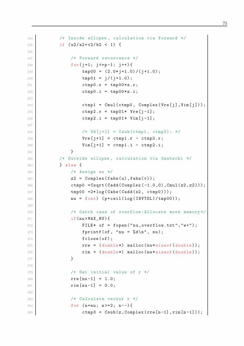
75
244 /* Inside ellipse , calculation via forward */
245 if (u2/a2+v2/b2 < 1) {
246
247 /* Forward recurrence */
248 for(j=1; j<=p-1; j++){
249 tmp00 = (2.0*j+1.0)/(j+1.0);
250 tmp01 = j/(j+1.0);
251 ctmp0.r = tmp00*z.r;
252 ctmp0.i = tmp00*z.i;
253
254 ctmp1 = Cmul(ctmp0 , Complex(Vre[j],Vim[j]));
255 ctmp2.r = tmp01* Vre[j-1];
256 ctmp2.i = tmp01* Vim[j-1];
257
258 /* Vd[j+1] = Csub(ctmp1 , ctmp2); */
259 Vre[j+1] = ctmp1.r - ctmp2.r;
260 Vim[j+1] = ctmp1.i - ctmp2.i;
261 }
262 /* Outside ellipse , calculation via Gautschi */
263 } else {
264 /* Assign nu */
265 z2 = Complex(fabs(u),fabs(v));
266 ctmp0 =Csqrt(Cadd(Complex (-1.0,0),Cmul(z2,z2)));
267 tmp00 =2*log(Cabs(Cadd(z2, ctmp0)));
268 nu = (int) (p+ceil(log(INVTOL)/tmp00));
269
270 /* Catch case of overflow :Allocate more memory*/
271 if(nu>MAX_NU){
272 FILE* of = fopen("nu_overflow.txt","w+");
273 fprintf(of, "nu = %d\n", nu);
274 fclose(of);
275 rre = (double*) malloc(nu*sizeof(double));
276 rim = (double*) malloc(nu*sizeof(double));
277 }
278
279 /* Set initial value of r */
280 rre[nu -1] = 1.0;
281 rim[nu -1] = 0.0;
282
283 /* Calculate vector r */
284 for (n=nu; n>=2; n--){
285 ctmp3 = Csub(z,Complex(rre[n-1],rim[n-1]));

76 Appendix B: The file ’liblegfct.c’
286 tmp00 = (n*n)/((4*n*n-1.0)*(ctmp3.r*ctmp3.r
287 +ctmp3.i*ctmp3.i));
288 rre[n-2] = tmp00*ctmp3.r;
289 rim[n-2] = -tmp00*ctmp3.i;
290 }
291
292 /* Calculate the remaining values of V */
293 for (n=2; n<p+1; n++){
294 ctmp3 = Cmul(Complex(rre[n-2],rim[n-2]),
295 Complex(Vre[n-1],Vim[n-1]));
296 tmp00 = (2*n-1.0)/(n);
297 Vre[n] = tmp00*ctmp3.r;
298 Vim[n] = tmp00*ctmp3.i;
299 }
300 }/* end else */
301 }/* end if p > 1 */
302 }/* end qt0 */
303
304 /* qt1
305 *
306 * INPUT: z (point of evaluation)
307 * p (max. polynomial degree)
308 * fac (factor to multiply )
309 * rretmp (temporary variables)
310 * rimtmp (temporary variables)
311 * OUTPUT: Vre (real part of the integral )
312 * Vim (imaginary part of the integral )
313 *
314 * / 1
315 * |
316 * fac * | P_k(t) / (z-t)^2 dt; z = u+iv, k = 0,..., p
317 * |
318 * / -1
319 *
320 * where P_k(t) are the Legendre polynomials.
321 *
322 */
323
324 void qt1(fcomplex const z, int const p, double const fac,
325 double *rretmp , double *rimtmp ,
326 double *Vre , double *Vim){
327

77
328 int j,n,nu;
329 double tmp00 , tmp01;
330 double a2, u, u2, v, v2, b, b2;
331 fcomplex c1,c2,c3,z2, ctmp0 , ctmp1 , ctmp2 , ctmp3;
332 double *rre = rretmp;
333 double *rim = rimtmp;
334
335 /* Get real(z) and imag(z) */
336 u = z.r;
337 v = z.i;
338 u2 = u*u;
339 v2 = v*v;
340
341 /* Set V[0] and V[1] */
342 /* case: z is complex */
343 if ( v2 > eps ){
344 c1 = Csub(Cmul(z,z),Complex (1.0,0.0));
345 c2 = Cdiv(Complex (2.0 ,0),c1);
346 Vre[0] = c2.r;
347 Vim[0] = c2.i;
348 if(p>0){
349 c3=Clog(Cdiv(Complex(u+1.0,v),Complex(u-1.0,v)));
350 ctmp0 = Csub(Cmul(z,c2),c3);
351 Vre[1] = ctmp0.r;
352 Vim[1] = ctmp0.i;
353 }
354 /* case: z is real and in (-1,1) */
355 } else if(u2!=1){
356 Vre[0] = 2.0/(u2 -1);
357 Vim[0] = 0.0;
358 if(p>0){
359 Vre[1] = 2.0*u/(u2 -1) - log(fabs((u+1)/(u-1)));
360 Vim[1] = 0.0;
361 }
362 /* case: z is real , z = +/- 1
363 * Integral has singularity set V[j] = 0 for all j.
364 */
365 } else {
366 for(j=0; j<=p; j++){
367 Vre[j] = 0.0;
368 Vim[j] = 0.0;
369 }

78 Appendix B: The file ’liblegfct.c’
370 return;
371 }
372
373 /* Multiply with fac */
374 Vre[0] *= fac;
375 Vim[0] *= fac;
376 if(p>0){
377 Vre[1] *= fac;
378 Vim[1] *= fac;
379 }
380
381 /* Calculate V[2]..V[p] */
382 if(p>1){
383 /* Ellipse parameters */
384 b = MIN(1 ,4.5/ pow(p+1.0,1.17));
385 b2 = b*b;
386 a2 = 1.0+b2;
387
388 /* Inside ellipse , calculation via forward */
389 if (u2/a2+v2/b2 < 1) {
390
391 /* Forward recurrence */
392 for(j=1; j<=p-1; j++){
393 tmp00 = (2.0*j+1.0)/j;
394 tmp01 = (j+1.0)/j;
395 ctmp0.r = tmp00*z.r;
396 ctmp0.i = tmp00*z.i;
397
398 ctmp1 = Cmul(ctmp0 , Complex(Vre[j],Vim[j]));
399 ctmp2.r = tmp01* Vre[j-1];
400 ctmp2.i = tmp01* Vim[j-1];
401
402 Vre[j+1] = ctmp1.r - ctmp2.r;
403 Vim[j+1] = ctmp1.i - ctmp2.i;
404 }
405 /* Outside ellipse , calculation via Gautschi */
406 } else {
407 /* Assign nu */
408 z2 = Complex(fabs(u),fabs(v));
409 ctmp0 = Csqrt(Cadd(Complex (-1.0,0), Cmul(z2,z2))
);
410 tmp00 = 2*log(Cabs(Cadd(z2, ctmp0)));

79
411 nu = (int) (p+ceil(log(INVTOL)/tmp00));
412
413 /* Catch case of overflow :Allocate more memory*/
414 if(nu>MAX_NU){
415 FILE* of = fopen("nu_overflow.txt","w+");
416 fprintf(of, "nu = %d\n", nu);
417 fclose(of);
418 rre = (double*) malloc(nu*sizeof(double));
419 rim = (double*) malloc(nu*sizeof(double));
420 }
421
422
423 /* Set initial value of r */
424 rre[nu -1] = 1.0;
425 rim[nu -1] = 0.0;
426
427 /* Calculate vector r */
428 for (n=nu; n>=2; n--){
429 ctmp3 = Csub(z,Complex(rre[n-1],rim[n-1]));
430 tmp00 = (n*n-1.0) /((4*n*n-1.0)*
431 (ctmp3.r*ctmp3.r+ctmp3.i*ctmp3.i));
432 rre[n-2] = tmp00*ctmp3.r;
433 rim[n-2] = -tmp00*ctmp3.i;
434 }
435
436 /* Calculate the remaining values of V */
437 for (n=2; n<p+1; n++){
438 ctmp3 = Cmul(Complex(rre[n-2],rim[n-2]),
439 Complex(Vre[n-1],Vim[n-1]));
440 tmp00 = (2*n-1.0)/(n-1.0);
441 Vre[n] = tmp00*ctmp3.r;
442 Vim[n] = tmp00*ctmp3.i;
443 }
444
445 }/* end else */
446
447 }/* end if p > 1 */
448 }/* end qt1 */
449
450 /* qtn
451 *
452 * INPUT: z (point of evaluation)

80 Appendix B: The file ’liblegfct.c’
453 * p (max. polynomial degree)
454 * n (max. exponent of (z-t)^n)
455 * fac (factor to multiply )
456 * rretmp (temporary variables)
457 * rimtmp (temporary variables)
458 * Vtmpre (temporary variables)
459 * Vtmpim (temporary variables)
460 * OUTPUT: Vre (real part of the integral )
461 * Vim (imaginary part of the integral )
462
463 * / 1
464 * |
465 * fac * | P_k(t) * log(t-z) dt; z = u+iv, k = 0,...,p
466 * |
467 * / -1
468 * and for j = 0..n
469 * / 1
470 * |
471 * fac * | P_k(t) / (z-t)^j dt; z = u+iv, k = 0,...,p
472 * |
473 * / -1
474 *
475 * where P_k(t) are the Legendre polynomials.
476 *
477 */
478
479 void qtn(fcomplex const z, int const p, int const n,
480 double const fac , double *rretmp , double *rimtmp ,
481 double *Vtmpre , double *Vtmpim ,
482 double *Vre , double *Vim){
483
484 int k,i;
485 double u,u2,v2,ar,br;
486 fcomplex z2, a,b, ctmp , ctmp1 , ctmp2 , ctmp3;
487
488 /* Get real(z) and imag(z) */
489 z2 = Cmul(z,z);
490 u = z.r;
491 u2 = u*u;
492 v2 = z.i * z.i;
493 ctmp = Complex(z2.r-1.0,z2.i);
494

81
495 /* Set qt0 V */
496 qt0(z,p,fac ,rretmp ,rimtmp ,Vtmpre ,Vtmpim);
497 for (k=0;k<p+1;k++) {
498 Vre[k] = Vtmpre[k];
499 Vim[k] = Vtmpim[k];
500 }
501
502 /* Set qt1 V */
503 if (n>0) {
504 qt1(z,p,fac ,rretmp ,rimtmp ,Vtmpre ,Vtmpim);
505 for (k=0;k<p+1;k++) {
506 Vre[k+p+1] = Vtmpre[k];
507 Vim[k+p+1] = Vtmpim[k];
508 }
509 }
510
511 if (n>1) {
512 /* Loop for calculation of qti upto degree p*/
513 for (k=0;k<p+1;k++) {
514 /* Loop for caluclation upto qtn */
515 for (i=1;i<n;i++) {
516 /* case: z is complex */
517 if (v2 > eps) {
518 a = Cdiv(RCmul(2*i,z),RCmul(i+1,ctmp));
519 b = Cdiv( RCmul((k-i+1.0)*(k+i),
520 Complex (1.0 ,0)),
521 RCmul(i*(i+1.0),ctmp));
522 ctmp1 = Cmul(a,Complex(Vre[k+i*(p+1)],
523 Vim[k+i*(p+1)]));
524 ctmp2=Cmul(b,Complex(Vre[k+(i-1)*(p+1)],
525 Vim[k+(i-1)*(p+1)]));
526 ctmp3 = Cadd(ctmp1 ,ctmp2);
527 Vre[k+(i+1)*(p+1)] = ctmp3.r;
528 Vim[k+(i+1)*(p+1)] = ctmp3.i;
529 /* case: z is real and not +1 or -1*/
530 } else if (u2 != 1) {
531 ar = 2.0*i*u / ((i+1)*(u2 -1.0));
532 br = (k-i+1.0)*(k+i) /
533 (i*(i+1.0)*(u2 -1.0));
534 Vre[k+(i+1)*(p+1)] = ar*Vre[k+i*(p+1)]
535 + br*Vre[k+(i-1)*(p+1)];
536 Vim[k+(i+1)*(p+1)] = 0.0;

82 Appendix B: The file ’liblegfct.c’
537
538 /* case: z = +1 or z = -1 */
539 } else {
540 Vre[k+(i+1)*(p+1)] = 0.0;
541 Vim[k+(i+1)*(p+1)] = 0.0;
542 }
543 }
544 }
545 }
546 }/* end qtn */
547
548 /* q0
549 *
550 * INPUT: z (point of evaluation)
551 * p (max. polynomial degree)
552 * fac (factor to multiply )
553 * rretmp (temporary variables)
554 * rimtmp (temporary variables)
555 * OUTPUT: Vre (real part of the integral )
556 * Vim (imaginary part of the integral )
557 *
558 * / 1
559 * |
560 * fac * 0.5 * | P_k(t) / (z-t) dt; z = u+iv, k = 0,...,p
561 * |
562 * / -1
563 *
564 * where P_k(t) are the Legendre polynomials.
565 *
566 */
567
568 void q0(fcomplex const z, int const p, double const fac ,
569 double *rretmp , double *rimtmp ,
570 double *Vre , double *Vim){
571
572 int k;
573 /* Get qt0 */
574 qt0(z,p,fac ,rretmp ,rimtmp ,Vre ,Vim);
575
576 /* Multiply V with 0.5 and fac */
577 for (k=0;k<p+1;k++) {
578 Vre[k] = fac *0.5*Vre[k];

83
579 Vim[k] = fac *0.5*Vim[k];
580 }
581 }
582
583 /* q1
584 *
585 * INPUT: z (point of evaluation)
586 * p (max. polynomial degree)
587 * fac (factor to multiply )
588 * rretmp (temporary variables)
589 * rimtmp (temporary variables)
590 * OUTPUT: Vre (real part of the integral )
591 * Vim (imaginary part of the integral )
592 *
593 * / 1
594 * |
595 * fac * -0.5*(z^2-1)^(1/2) * | P_k(t)/(z-t)^2 dt;
596 * |
597 * / -1
598 * for z = u+iv, k = 0, ..., p, or
599 * / 1
600 * |
601 * fac * 0.5*(1 -x^2) ^(1/2) * | P_k(t)/(x-t)^2 dt;
602 * |
603 * / -1
604 * for |x| < 1 real ,k = 0,...,p and
605 * where P_k(t) are the Legendre polynomials.
606 *
607 */
608
609 void q1(fcomplex const z, int const p, double const fac ,
610 double *rretmp , double *rimtmp ,
611 double *Vre , double *Vim){
612
613 int k;
614 double u,v,v2,u2,tmp;
615 fcomplex z2, z_tmp , ctmp , ctmp2;
616
617 /* Get real(z) and imag(z) */
618 u = z.r;
619 v = z.i;
620 u2 = u*u;

84 Appendix B: The file ’liblegfct.c’
621 v2 = v*v;
622 z2 = Cmul(z,z);
623
624 /* Get qt1 */
625 qt1(z,p,fac ,rretmp ,rimtmp ,Vre ,Vim);
626
627 /* Multiply V with factor*/
628 for (k=0;k<p+1;k++) {
629 /* z is complex and not in [-1,1] */
630 if (v2 > eps || u2 > 1) {
631 z_tmp = Complex(Vre[k],Vim[k]);
632 ctmp = RCmul(-0.5*fac ,
633 Csqrt(Complex(z2.r-1.0,z2.i)));
634 ctmp2 = Cmul(z_tmp ,ctmp);
635 Vre[k] = ctmp2.r;
636 Vim[k] = ctmp2.i;
637 }
638 /* z is real and |z| < 1*/
639 else {
640 tmp = sqrt(1-u2)/2;
641 Vre[k] = fac*tmp*Vre[k];
642 Vim[k] = fac*tmp*Vim[k];
643 }
644 }
645 }
646
647 /* qn
648 *
649 * INPUT: z (point of evaluation)
650 * p (max. polynomial degree)
651 * n (upper limit of calculation of qn)
652 * fac (factor to multiply )
653 * rretmp (temporary variables)
654 * rimtmp (temporary variables)
655 * Vtmore (temporary variables)
656 * Vtmpim (temporary variables)
657 * OUTPUT: Vre (real part of the integral )
658 * Vim (imaginary part of the integral )
659 *
660 * / 1
661 * |
662 * fac * -0.5*(z^2-1)^(1/2) * | P_k(t)/(z-t)^m dt;

85
663 * |
664 * / -1
665 * for z = u+iv, k = 0, ..., p, or
666 * / 1
667 * |
668 * fac * 0.5*(1 -x^2) ^(1/2) * | P_k(t)/(x-t)^m dt;
669 * |
670 * / -1
671 * for |x| < 1 real ,k = 0,...,p, m = 0..n and
672 * where P_k(t) are the Legendre polynomials.
673 *
674 */
675
676 void qn(fcomplex const z, int const p, int const n,
677 double const fac , double *rretmp , double *rimtmp ,
678 double *Vtmpre , double *Vtmpim ,
679 double *Vre , double *Vim){
680
681 int k,i;
682 double u,u2,v2,ar,br;
683 fcomplex z2, a,b, ctmp , ctmp1 , ctmp2 , ctmp3;
684
685 /* Get real(z) and imag(z) */
686 z2 = Cmul(z,z);
687 u = z.r;
688 u2 = u*u;
689 v2 = z.i * z.i;
690 ctmp = Csqrt(Complex(z2.r-1.0,z2.i));
691
692 /* Set q0 -> V */
693 q0(z,p,fac,rretmp ,rimtmp ,Vtmpre ,Vtmpim);
694 for (k=0;k<p+1;k++) {
695 Vre[k] = Vtmpre[k];
696 Vim[k] = Vtmpim[k];
697 }
698
699 /* Set q1 -> V */
700 if (n>0) {
701 q1(z,p,fac ,rretmp ,rimtmp ,Vtmpre ,Vtmpim);
702 for (k=0;k<p+1;k++) {
703 Vre[k+p+1] = Vtmpre[k];
704 Vim[k+p+1] = Vtmpim[k];

86 Appendix B: The file ’liblegfct.c’
705 }
706 }
707
708 if (n>1) {
709 /* Loop for calculation of qi upto degree p*/
710 for (k=0;k<p+1;k++) {
711 /* Loop for caluclation upto qn */
712 for (i=0;i<n-1;i++) {
713 /* case: z is complex */
714 if (v2 > eps) {
715 a = Cdiv(RCmul( -2.0*(i+1),z),ctmp);
716 b = Complex ((k-i)*(k+i+1.0) ,0.0);
717 ctmp1=Cmul(a,Complex(Vre[k+(i+1)*(p+1)],
718 Vim[k+(i+1)*(p+1)]));
719 ctmp2 = Cmul(b,Complex(Vre[k+i*(p+1)],
720 Vim[k+i*(p+1)]));
721 ctmp3 = Cadd(ctmp1 ,ctmp2);
722 Vre[k+(i+2)*(p+1)] = ctmp3.r;
723 Vim[k+(i+2)*(p+1)] = ctmp3.i;
724 /* case: z is real and not in [-1,1] */
725 } else if (u2 > 1) {
726 ar = -2.0*(i+1)*u / sqrt(u2 -1.0);
727 br = (k+i+1.0)*(k-i);
728 Vre[k+(i+2)*(p+1)]=ar*Vre[k+(i+1)*(p+1)]
729 + br*Vre[k+i*(p+1)];
730 Vim[k+(i+2)*(p+1)] = 0.0;
731 /* case: z is real and in (-1,1) */
732 } else if (u2 < 1) {
733 ar = -2.0*(i+1)*u / sqrt(1.0-u2);
734 br = (k+i+1.0)*(k-i);
735 Vre[k+(i+2)*(p+1)]=ar*Vre[k+(i+1)*(p+1)]
736 - br*Vre[k+i*(p+1)];
737 Vim[k+(i+2)*(p+1)] = 0.0;
738 /* case: z = +1 or z = -1 */
739 } else {
740 Vre[k+(i+2)*(p+1)] = 0.0;
741 Vim[k+(i+2)*(p+1)] = 0.0;
742 }
743 }
744 }
745 }
746 }/* end qn */

87
747
748
749 /* r0
750 *
751 * INPUT: z (point of evaluation)
752 * fac (factor to multiply )
753 * p (max. polynomial degree)
754 * rretmp (temporary variables)
755 * rimtmp (temporary variables)
756 * OUTPUT: Vre (real part of the integral )
757 * Vim (imaginary part of the integral )
758 *
759 * / 1
760 * | N_k(t)
761 * fac * | -------- dt; z = u+iv, k = 1,..., p
762 * | z-t
763 * / -1
764 *
765 * / t
766 * where N_k(t) = | P_(k-2)(xsi) dxsi
767 * -1 /
768 *
769 *
770 */
771
772 void r0(fcomplex const z, int const p, double const fac ,
773 double *rretmp , double *rimtmp ,
774 double *Vre , double *Vim){
775
776 int j,n,nu;
777 double tmp00 , tmp01;
778 double a1, a2, u, u2, v, v2, b, b2;
779 fcomplex c1,c2,c3,z2, ctmp0 , ctmp1 , ctmp2 , ctmp3;
780 double *rre = rretmp;
781 double *rim = rimtmp;
782
783 /* Get real(z) and imag(z) */
784 u = z.r;
785 v = z.i;
786 u2 = u*u;
787 v2 = v*v;
788

88 Appendix B: The file ’liblegfct.c’
789 /* Set initial values V[0], V[1] and V[2] */
790 /* case: z is complex */
791 if ( v2 > eps ){
792 c1 = Clog(Complex( z.r+1.0, z.i));
793 c2 = Clog(Complex( z.r-1.0, z.i));
794 c3 = RCmul(0.5,Csub(c1,c2));
795
796 ctmp0 = Cmul(c3,Complex(-z.r+1.0,-z.i));
797 ctmp1 = Cmul(c3,Complex(z.r+1.0,z.i));
798 Vre[0] = ctmp0.r + 1.0;
799 Vim[0] = ctmp0.i;
800 Vre[1] = ctmp1.r - 1.0;
801 Vim[1] = ctmp1.i;
802 if(p>1){
803 ctmp0 = Csub(Cmul(c3,Csub(Cmul(z,z),
804 Complex (1.0,0.0))),z);
805 Vre[2] = ctmp0.r;
806 Vim[2] = ctmp0.i;
807 }
808 /* case: z is real and z != +/- 1 */
809 } else if(u2!=1){
810 a1= 0.5*log(fabs((1.0+u)/(u-1.0)));
811
812 Vre[0] = a1*(1.0-u)+1.0;
813 Vim[0] = 0.0;
814 Vre[1] = a1*(1.0+u) -1.0;
815 Vim[1] = 0.0;
816 if(p>1){
817 Vre[2] = (u2 -1.0)*a1-u;
818 Vim[2] = 0.0;
819 }
820 /* case: z = 1*/
821 } else if(u == 1.0) {
822 Vre[0] = 1.0;
823 Vim[0] = 0.0;
824
825 Vre[1] = BIG;
826 Vim[1] = 0.0;
827
828 if(p>1){
829 Vre[2] = -u;
830 Vim[2] = 1.0;

89
831 }
832 /* case: z = -1*/
833 } else if(u == -1.0) {
834 Vre[0] = -BIG;
835 Vim[0] = 0.0;
836
837 Vre[1] = -1.0;
838 Vim[1] = 0.0;
839
840 if(p>1){
841 Vre[2] = -u;
842 Vim[2] = 0.0;
843 }
844 }
845
846
847 /* Multiply with fac */
848 Vre[0] *= fac;
849 Vim[0] *= fac;
850 Vre[1] *= fac;
851 Vim[1] *= fac;
852 if(p>1){
853 Vre[2] *= fac;
854 Vim[2] *= fac;
855 }
856
857 /* Calculate the remaining values of V */
858 if(p>2){
859 /* Set V[3] */
860 ctmp0 = Cmul(z,Complex(Vre[2],Vim [2]));
861 Vre[3] = ctmp0.r + 2.0/3.0* fac;
862 Vim[3] = ctmp0.i;
863
864 if(p>3){
865 /* Ellipse parameter */
866 b = MIN(1 ,4.5/ pow(p+1.0 ,1.17));
867 b2 = b*b;
868 a2 = 1.0+b2;
869
870 /* Inside ellipse calculation via forward */
871 if (u2/a2+v2/b2 < 1) {
872 for(j=3; j<=p-1; j++){
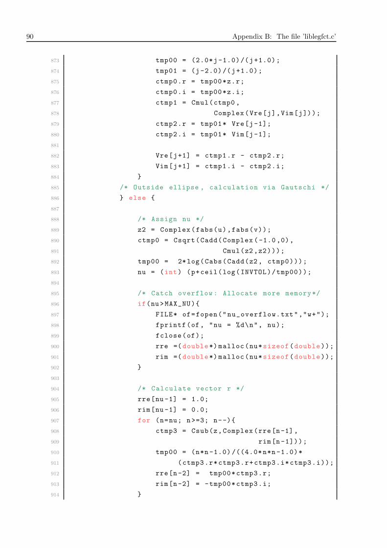
90 Appendix B: The file ’liblegfct.c’
873 tmp00 = (2.0*j-1.0)/(j+1.0);
874 tmp01 = (j-2.0)/(j+1.0);
875 ctmp0.r = tmp00*z.r;
876 ctmp0.i = tmp00*z.i;
877 ctmp1 = Cmul(ctmp0 ,
878 Complex(Vre[j],Vim[j]));
879 ctmp2.r = tmp01* Vre[j-1];
880 ctmp2.i = tmp01* Vim[j-1];
881
882 Vre[j+1] = ctmp1.r - ctmp2.r;
883 Vim[j+1] = ctmp1.i - ctmp2.i;
884 }
885 /* Outside ellipse , calculation via Gautschi */
886 } else {
887
888 /* Assign nu */
889 z2 = Complex(fabs(u),fabs(v));
890 ctmp0 = Csqrt(Cadd(Complex (-1.0,0),
891 Cmul(z2,z2)));
892 tmp00 = 2*log(Cabs(Cadd(z2, ctmp0)));
893 nu = (int) (p+ceil(log(INVTOL)/tmp00));
894
895 /* Catch overflow : Allocate more memory*/
896 if(nu>MAX_NU){
897 FILE* of=fopen("nu_overflow.txt","w+");
898 fprintf(of, "nu = %d\n", nu);
899 fclose(of);
900 rre =(double*) malloc(nu*sizeof(double));
901 rim =(double*) malloc(nu*sizeof(double));
902 }
903
904 /* Calculate vector r */
905 rre[nu -1] = 1.0;
906 rim[nu -1] = 0.0;
907 for (n=nu; n>=3; n--){
908 ctmp3 = Csub(z,Complex(rre[n-1],
909 rim[n-1]));
910 tmp00 = (n*n-1.0) /((4.0*n*n-1.0)*
911 (ctmp3.r*ctmp3.r+ctmp3.i*ctmp3.i));
912 rre[n-2] = tmp00*ctmp3.r;
913 rim[n-2] = -tmp00*ctmp3.i;
914 }

91
915
916 /* Calcualte vector V */
917 for (n=3; n<p; n++){
918 ctmp3 = Cmul(Complex(rre[n-2],rim[n-2]),
919 Complex(Vre[n],Vim[n]));
920 tmp00 = (2.0*n-1.0)/(n+1.0);
921 Vre[n+1] = tmp00*ctmp3.r;
922 Vim[n+1] = tmp00*ctmp3.i;
923 }
924 }
925 }/* endif p > 3 */
926 }/* endif p > 2 */
927 }/*end r0 */
928
929 /* r1
930 *
931 * INPUT: z (point of evaluation)
932 * fac (factor to multiply )
933 * p (max. polynomial degree)
934 * rretmp (temporary variables)
935 * rimtmp (temporary variables)
936 * OUTPUT: Vre (real part of the integral )
937 * Vim (imaginary part of the integral )
938 *
939 * / 1
940 * | N_k(t)
941 * fac * | ----------- dt; z = u+iv, k = 1, ..., p
942 * | (z-t)^2
943 * / -1
944 *
945 * / t
946 * where N_j(t) = | P_(k-2)(xsi) dxsi
947 * -1 /
948 *
949 *
950 */
951
952 void r1(fcomplex const z, int const p, double const fac ,
953 double *rretmp , double *rimtmp ,
954 double *Vre , double *Vim){
955
956 int j,n,nu;

92 Appendix B: The file ’liblegfct.c’
957 double tmp00 , tmp01;
958 double a1, a2, a3, u, u2, v, v2, b, b2;
959 fcomplex c1,c2,c3,c4,c5,z2, ctmp0 , ctmp1 , ctmp2 , ctmp3;
960 double *rre = rretmp;
961 double *rim = rimtmp;
962
963 /* Get real(z) and imag(z) */
964 u = z.r;
965 v = z.i;
966 u2 = u*u;
967 v2 = v*v;
968
969 /* Set initial values V[0], V[1], V[2] and V[3]*/
970 /* case: z is complex */
971 if ( v2 > eps ){
972 c1=Cdiv(Complex (1.0,0.0),Complex(u+1.0,v));
973 c2=Cdiv(Complex (1.0,0.0),Complex(u-1.0,v));
974 c3=Csub(c2,c1);
975 c4=Clog(Complex(-u+1,-v));
976 c5=Clog(Complex(-u-1,-v));
977 ctmp0 = Csub(RCmul(0.5,Csub(c5,c4)),c1);
978 ctmp1 = Csub(c2,RCmul(0.5,Csub(c5,c4)));
979
980 Vre[0] = ctmp0.r;
981 Vim[0] = ctmp0.i;
982 Vre[1] = ctmp1.r;
983 Vim[1] = ctmp1.i;
984 if(p>1){
985 ctmp0 = RCmul(-1.0,Cmul(z,Csub(c5,c4)));
986 Vre[2] = ctmp0.r + 2.0;
987 Vim[2] = ctmp0.i;
988 }
989 if(p>2){
990 ctmp0 = Cadd(RCmul(3.0,z),
991 Cmul(Csub(Complex (0.5,0.0),
992 RCmul(1.5,Cmul(z,z))),Csub(c5,c4)));
993 Vre[3] = ctmp0.r;
994 Vim[3] = ctmp0.i;
995 }
996 /* case: z is real , z != +/- 1 */
997 } else if(u2!=1){
998 a1 = u+1;

93
999 a2 = u-1;
1000 a3 = log(fabs(a1/a2));
1001
1002 Vre[0] = -1/a1+0.5*a3;
1003 Vim[0] = 0.0;
1004 Vre[1] = 1/a2 - 0.5*a3;
1005 Vim[1] = 0.0;
1006 if(p>1){
1007 Vre[2] = -u*a3+2.0;
1008 Vim[2] = 0.0;
1009 }
1010 if(p>2){
1011 Vre[3] = (0.5-1.5*u2)*a3+3*u;
1012 Vim[3] = 0.0;
1013 }
1014 /* case: z = 1 */
1015 } else if(u==1){
1016 Vre[0] = -0.5;
1017 Vim[0] = 0.0;
1018 Vre[1] = 0.0;
1019 Vim[1] = 0.0;
1020 if(p>1){
1021 Vre[2] = 2.0;
1022 Vim[2] = 0.0;
1023 }
1024 if(p>2){
1025 Vre[3] = 3.0;
1026 Vim[3] = 0.0;
1027 }
1028 /* otherwise */
1029 } else {
1030 Vre[0] = 0.0;
1031 Vim[0] = 0.0;
1032 Vre[1] = -0.5;
1033 Vim[1] = 0.0;
1034 if(p>1){
1035 Vre[2] = 2.0;
1036 Vim[2] = 0.0;
1037 }
1038 if(p>2){
1039 Vre[3] = -3.0;
1040 Vim[3] = 0.0;

94 Appendix B: The file ’liblegfct.c’
1041 }
1042 }
1043
1044 /* Multiply with factor */
1045 Vre[0] *= fac;
1046 Vim[0] *= fac;
1047 if(p>0){
1048 Vre[1] *= fac;
1049 Vim[1] *= fac;
1050 }
1051 if(p>1){
1052 Vre[2] *= fac;
1053 Vim[2] *= fac;
1054 }
1055 if(p>2){
1056 Vre[3] *= fac;
1057 Vim[3] *= fac;
1058 }
1059
1060 /* Calculate the remaining values of V */
1061 if(p>3){
1062
1063 /* Ellipse parameter */
1064 b = MIN(1 ,4.5/ pow(p+1.0,1.17));
1065 b2 = b*b;
1066 a2 = 1.0+b2;
1067
1068 /* Inside ellipse calculation via forward */
1069 if (u2/a2+v2/b2 < 1) {
1070 /* Forward recurrence */
1071 for(j=3; j<=p-1; j++){
1072 tmp00 = (2.0*j-1.0)/j;
1073 tmp01 = (j-1.0)/j;
1074 ctmp0.r = tmp00*z.r;
1075 ctmp0.i = tmp00*z.i;
1076
1077 ctmp1 = Cmul(ctmp0 , Complex(Vre[j],Vim[j]));
1078 ctmp2.r = tmp01* Vre[j-1];
1079 ctmp2.i = tmp01* Vim[j-1];
1080
1081 Vre[j+1] = ctmp1.r - ctmp2.r;
1082 Vim[j+1] = ctmp1.i - ctmp2.i;

95
1083 }
1084 } else {
1085
1086 /* Assign nu */
1087 z2 = Complex(fabs(u),fabs(v));
1088 ctmp0= Csqrt(Cadd(Complex (-1.0,0),Cmul(z2,z2)));
1089 tmp00 = 2*log(Cabs(Cadd(z2, ctmp0)));
1090 nu = (int) (p+ceil(log(INVTOL)/tmp00));
1091
1092 /* Catch case of overflow :Allocate more memory*/
1093 if(nu>MAX_NU){
1094 FILE* of = fopen("nu_overflow.txt","w+");
1095 fprintf(of, "nu = %d\n", nu);
1096 fclose(of);
1097 rre = (double*) malloc(nu*sizeof(double));
1098 rim = (double*) malloc(nu*sizeof(double));
1099 }
1100
1101 /* Calculate vector r */
1102 rre[nu -1] = 1.0;
1103 rim[nu -1] = 0.0;
1104 for (n=nu; n>=3; n--){
1105 ctmp3 = Csub(z,Complex(rre[n-1],rim[n-1]));
1106 tmp00 = (n*n)/((4.0*n*n-1.0)*
1107 (ctmp3.r*ctmp3.r + ctmp3.i*ctmp3.i));
1108 rre[n-2] = tmp00*ctmp3.r;
1109 rim[n-2] = -tmp00*ctmp3.i;
1110
1111 }
1112
1113 /* Calculate vector V */
1114 for (n=3; n<p; n++){
1115 ctmp3 = Cmul(Complex(rre[n-2],rim[n-2]),
1116 Complex(Vre[n],Vim[n]));
1117 tmp00 = (2*n-1.0)/(n);
1118 Vre[n+1] = tmp00*ctmp3.r;
1119 Vim[n+1] = tmp00*ctmp3.i;
1120 }
1121 }/* end else */
1122 }/* end if p > 3 */
1123 }/*end r1*/

96 Appendix B: The file ’liblegfct.c’
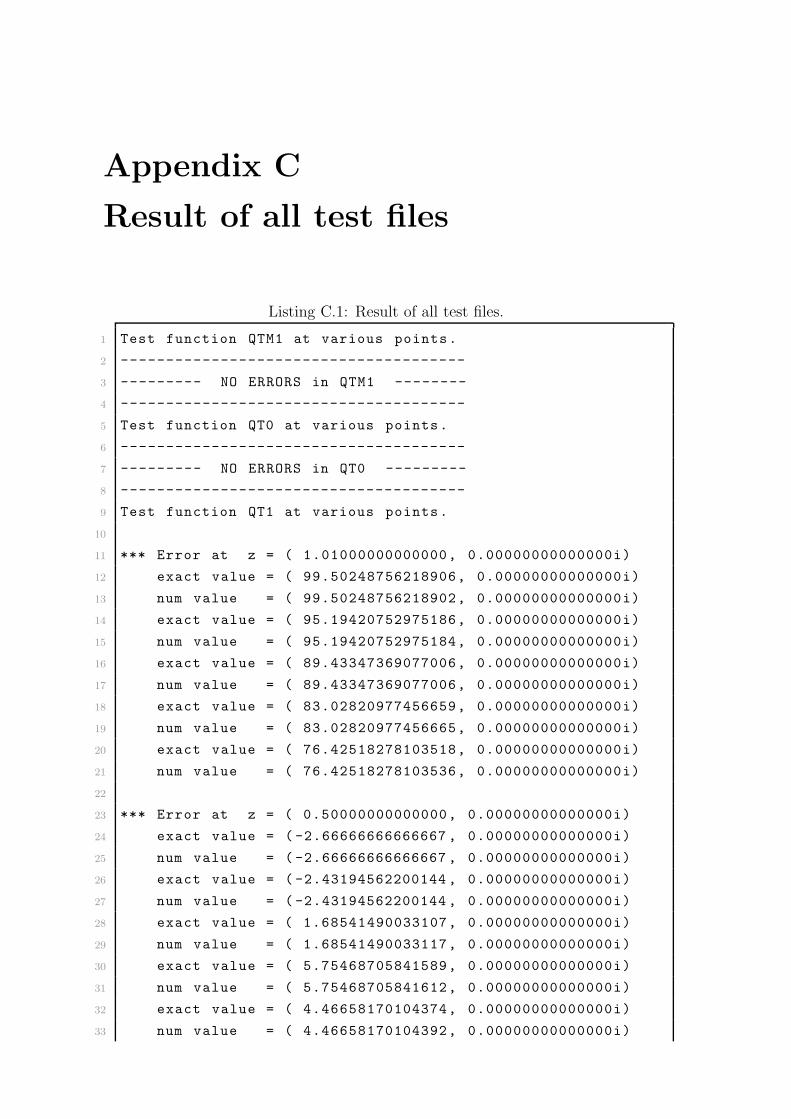
Appendix C
Result of all test files
Listing C.1: Result of all test files.
1 Test function QTM1 at various points.
2 --------------------------------------
3 --------- NO ERRORS in QTM1 --------
4 --------------------------------------
5 Test function QT0 at various points.
6 --------------------------------------
7 --------- NO ERRORS in QT0 ---------
8 --------------------------------------
9 Test function QT1 at various points.
10
11 *** Error at z = ( 1.01000000000000, 0.00000000000000i)
12 exact value = ( 99.50248756218906, 0.00000000000000i)
13 num value = ( 99.50248756218902, 0.00000000000000i)
14 exact value = ( 95.19420752975186, 0.00000000000000i)
15 num value = ( 95.19420752975184, 0.00000000000000i)
16 exact value = ( 89.43347369077006, 0.00000000000000i)
17 num value = ( 89.43347369077006, 0.00000000000000i)
18 exact value = ( 83.02820977456659, 0.00000000000000i)
19 num value = ( 83.02820977456665, 0.00000000000000i)
20 exact value = ( 76.42518278103518, 0.00000000000000i)
21 num value = ( 76.42518278103536, 0.00000000000000i)
22
23 *** Error at z = ( 0.50000000000000, 0.00000000000000i)
24 exact value = ( -2.66666666666667 , 0.00000000000000i)
25 num value = ( -2.66666666666667 , 0.00000000000000i)
26 exact value = ( -2.43194562200144 , 0.00000000000000i)
27 num value = ( -2.43194562200144 , 0.00000000000000i)
28 exact value = ( 1.68541490033107, 0.00000000000000i)
29 num value = ( 1.68541490033117, 0.00000000000000i)
30 exact value = ( 5.75468705841589, 0.00000000000000i)
31 num value = ( 5.75468705841612, 0.00000000000000i)
32 exact value = ( 4.46658170104374, 0.00000000000000i)
33 num value = ( 4.46658170104392, 0.00000000000000i)

98 Appendix C: Result of all test files
34
35 *** Error at z = ( -0.14285714285714 , 0.00000000000000i)
36 exact value = ( -2.04166666666667 , 0.00000000000000i)
37 num value = ( -2.04166666666667 , 0.00000000000000i)
38 exact value = ( 0.57934873911845, 0.00000000000000i)
39 num value = ( 0.57934873911845, 0.00000000000000i)
40 exact value = ( 3.83504101656819, 0.00000000000000i)
41 num value = ( 3.83504101656828, 0.00000000000000i)
42 exact value = ( -2.23868061459485 , 0.00000000000000i)
43 num value = ( -2.23868061459491 , 0.00000000000000i)
44 exact value = ( -4.36716115055921 , 0.00000000000000i)
45 num value = ( -4.36716115055941 , 0.00000000000000i)
46
47 --------- ERRORS in QT1.
48 Test function QTN(2) at various points.
49
50 *** Error at z = ( 1.01000000000000, 0.00000000000000i)
51 exact value = ( 4999.87624068711193, 0.00000000000000i)
52 num value = ( 4999.87624068710829, 0.00000000000000i)
53 exact value = ( 4950.37251553179340, 0.00000000000000i)
54 num value = ( 4950.37251553179067, 0.00000000000000i)
55 exact value = ( 4857.08492939248390, 0.00000000000000i)
56 num value = ( 4857.08492939248208, 0.00000000000000i)
57 exact value = ( 4726.78883130486884, 0.00000000000000i)
58 num value = ( 4726.78883130486975, 0.00000000000000i)
59 exact value = ( 4566.48619518150099, 0.00000000000000i)
60 num value = ( 4566.48619518150826, 0.00000000000000i)
61
62 *** Error at z = ( 0.50000000000000, 0.00000000000000i)
63 exact value = ( 1.77777777777778, 0.00000000000000i)
64 num value = ( 1.77777777777778, 0.00000000000000i)
65 exact value = ( 3.55555555555556, 0.00000000000000i)
66 num value = ( 3.55555555555556, 0.00000000000000i)
67 exact value = ( 5.42569621077994, 0.00000000000000i)
68 num value = ( 5.42569621077994, 0.00000000000000i)
69 exact value = ( -0.65798169527213 , 0.00000000000000i)
70 num value = ( -0.65798169527236 , 0.00000000000000i)
71 exact value = ( -14.71570849367567 , 0.00000000000000i)
72 num value = ( -14.71570849367650 , 0.00000000000000i)
73
74 *** Error at z = ( -0.14285714285714 , 0.00000000000000i)
75 exact value = ( -0.29774305555556 , 0.00000000000000i)

99
76 num value = ( -0.29774305555556 , 0.00000000000000i)
77 exact value = ( 2.08420138888889, 0.00000000000000i)
78 num value = ( 2.08420138888889, 0.00000000000000i)
79 exact value = ( -1.16676616423323 , 0.00000000000000i)
80 num value = ( -1.16676616423323 , 0.00000000000000i)
81 exact value = ( -7.50340115253159 , 0.00000000000000i)
82 num value = ( -7.50340115253182 , 0.00000000000000i)
83 exact value = ( 6.66861598684874, 0.00000000000000i)
84 num value = ( 6.66861598684898, 0.00000000000000i)
85
86 --------- ERRORS in QTN(2).
87 Test function QTN(3) at various points.
88
89 *** Error at z = ( 1.10000000000000, 0.00000000000000i)
90 exact value = ( 333.29734010006121, 0.00000000000000i)
91 num value = ( 333.29734010006030, 0.00000000000000i)
92 exact value = ( 316.74045279487456, 0.00000000000000i)
93 num value = ( 316.74045279487370, 0.00000000000000i)
94 exact value = ( 287.94586617715868, 0.00000000000000i)
95 num value = ( 287.94586617715788, 0.00000000000000i)
96 exact value = ( 252.17525403238761, 0.00000000000000i)
97 num value = ( 252.17525403238685, 0.00000000000000i)
98 exact value = ( 214.07425898643254, 0.00000000000000i)
99 num value = ( 214.07425898643174, 0.00000000000000i)
100
101 *** Error at z = ( 0.50000000000000, 0.00000000000000i)
102 exact value = ( -2.76543209876543 , 0.00000000000000i)
103 num value = ( -2.76543209876543 , 0.00000000000000i)
104 exact value = ( -3.16049382716049 , 0.00000000000000i)
105 num value = ( -3.16049382716049 , 0.00000000000000i)
106 exact value = ( -6.32098765432099 , 0.00000000000000i)
107 num value = ( -6.32098765432099 , 0.00000000000000i)
108 exact value = ( -12.20332084512706 , 0.00000000000000i)
109 num value = ( -12.20332084512707 , 0.00000000000000i)
110 exact value = ( -4.78569703201935 , 0.00000000000000i)
111 num value = ( -4.78569703201880 , 0.00000000000000i)
112
113 *** Error at z = ( -0.14285714285714 , 0.00000000000000i)
114 exact value = ( -0.75262827932099 , 0.00000000000000i)
115 num value = ( -0.75262827932099 , 0.00000000000000i)
116 exact value = ( 0.40526138117284, 0.00000000000000i)
117 num value = ( 0.40526138117284, 0.00000000000000i)

100 Appendix C: Result of all test files
118 exact value = ( -2.83682966820988 , 0.00000000000000i)
119 num value = ( -2.83682966820988 , 0.00000000000000i)
120 exact value = ( 2.34987165489488, 0.00000000000000i)
121 num value = ( 2.34987165489488, 0.00000000000000i)
122 exact value = ( 14.67110635436383, 0.00000000000000i)
123 num value = ( 14.67110635436438, 0.00000000000000i)
124
125 --------- ERRORS in QTN(3).
126 Test function Q0 at various points.
127 --------------------------------------
128 --------- NO ERRORS in Q0 ---------
129 --------------------------------------
130 Test function Q1 at various points.
131 --------------------------------------
132 --------- NO ERRORS in Q1 ---------
133 --------------------------------------
134 Test function Q2 at various points.
135 --------------------------------------
136 --------- NO ERRORS in Q2 ---------
137 --------------------------------------
138 Test function Q3 at various points.
139
140 *** Error at z = ( 1.01000000000000, 0.00000000000000i)
141 exact value = ( -2849.66647171210616 , 0.00000000000000i)
142 num value = ( -2849.66647171210479 , 0.00000000000000i)
143 exact value = ( -2835.41919210819606 , 0.00000000000000i)
144 num value = ( -2835.41919210819515 , 0.00000000000000i)
145 exact value = ( -2807.34573476058995 , 0.00000000000000i)
146 num value = ( -2807.34573476058995 , 0.00000000000000i)
147 exact value = ( -2766.21382321825831 , 0.00000000000000i)
148 num value = ( -2766.21382321826059 , 0.00000000000000i)
149 exact value = ( -2713.05732158954697 , 0.00000000000000i)
150 num value = ( -2713.05732158955198 , 0.00000000000000i)
151
152 --------- ERRORS in Q3.
153 Test function R0 at various points.
154 --------------------------------------
155 --------- NO ERRORS in R0 ----------
156 --------------------------------------
157 Test function R1 at various points.
158 --------------------------------------
159 --------- NO ERRORS in R1 ----------

101
160 --------------------------------------

102 Appendix C: Result of all test files
Bibliography
[1] A. Bantle, M. Bantle, C. Erath, P. Heiter, and S. Funken. epsBEM - Effi-
cient and p-Stable Matlab Implementation of 2d BEM for Laplace and Lame
Problems. Technical report, Univeristy of Ulm, 2010 (in progress).
[2] Markus Bantle. Efficient Implementation of Collocation and Boundary Element
Methods for Integral Equations. Diplomarbeit, University of Ulm, May 2010.
[3] J.D. Donaldson and David Elliot. A Unified Approach to Quadrature Rules
with Asymptotic Estimates of their Remainders. SIAM Review, 9:24–82, 1972.
[4] David Elliot. Uniform Asymptotic Expansions of the Jacobi Polynomials and
an Associated Function. Mathematics of Computation, 25(114):309–315, April
1971.
[5] Walter Gautschi. Computational Aspects of Three-Term Recurrence Relations.
SIAM Review, 9(1):24–80, January 1967.
[6] Walter Gautschi. Minimal Solutions of Three-Term Recurrence Relation and
Orthogonal Polynomials. Mathematics of Computation, 36(154):547–554, April
1981.
[7] I.S. Gradstein and I.M. Ryshik. Summen-, Produkt- und Integraltafeln. Verlag
Harri Deutsch, 1981.
[8] M. Hermann. Numerische Mathematik. Oldenbourg Verlag Munchen Wien,
2006.
[9] Peter Deuflhard und Andreas Hohmann. Numerische Mathematik 1 - Eine
algorithmisch orientierte Einfuhrung. Walter de Gruyter, 2008.
[10] Robert Schaback und Holger Wendland. Numerische Mathematik. Springer-
Verlag Berlin-Heidelberg, 2005.
[11] Shanjie Zhang and Jianming Jin. Computation of Special Functions. Wiley-
Interscience publication, 1996.


Ehrenwortliche Erklarung
Ich erklare hiermit ehrenwortlich, dass ich die vorliegende Arbeit selbststandig
angefertigt habe. Die aus fremden Quellen direkt oder indirekt ubernommenen
Gedanken sind als solche kenntlich gemacht. Die Arbeit wurde bisher keiner an-
deren Prufungsbehorde vorgelegt und auch noch nicht veroffentlicht.
Ich bin mir bewusst, dass eine unwahre Erklarung rechtliche Folgen haben wird.
Ulm, den 14. Juni 2010
(Unterschrift)