Embed Size (px)
Citation preview
International Journal of Mass Spectrometry 228 (2003) 1–33
Review
Stable isotope ratio mass spectrometry in globalclimate change research
Prosenjit Ghosh, Willi A. Brand∗
Isotopen- und Gaslabor, Max-Planck-Institut für Biogeochemie, Postfach 100164, Jena 07701, Germany
Received 29 January 2003; accepted 20 May 2003
Abstract
Stable isotope ratios of the life science elements carbon, hydrogen, oxygen and nitrogen vary slightly, but significantly inmajor compartments of the earth. Owing mainly to antropogenic activities including land use change and fossil fuel burning,the 13C/12C ratio of CO2 in the atmosphere has changed over the last 200 years by 1.5 parts per thousand (from about0.0111073 to 0.0110906). In between interglacial warm periods and glacial maxima, the18O/16O ratio of precipitation inGreenland has changed by as much as 5 parts per thousand (0.001935–0.001925). While seeming small, such changes aredetectable reliably with specialised mass spectrometric techniques. The small changes reflect natural fractionation processesthat have left their signature in natural archives. These enable us to investigate the climate of past times in order to understandhow the Earth’s climatic system works and how it can react to external forcing. In addition, studying contemporary isotopicchange of natural compartments can help to identify sources and sinks for atmospheric trace gases provided the respectiveisotopic signatures are large enough for measurement and have not been obscured by unknown processes. This informationis vital within the framework of the Kyoto process for controlling CO2 emissions.© 2003 Elsevier B.V. All rights reserved.
Keywords: Climate change; Stable isotopes; Carbon cycle; Isotope ratio mass spectrometry
1. Introduction
Man has followed and tried to understand climatefor millenia, primarily driven by the need to assignthe appropriate times for sowing and harvesting or todetermine the timing for food and fuel storage neces-sary to survive during winter. Since our contemporary
∗ Corresponding author. Tel.:+49-3641-576400;fax: +49-3641-5770.
E-mail address: [email protected] (W.A. Brand).
well-being still depends upon climate to some extent,there is a growing need to predict its future develop-ment at a range of temporal scales, its variability andassociated potential hazards.
Owing to external forcing, the Earth’s climatic sys-tem has always seen large variations[1–3]. Predictionof future climatic conditions will become possible pro-vided we have a reasonably thorough understandingof the physico-chemical processes that are operatingon the Earth’s system. Detailed knowledge about thevariability of physical and chemical processes driving
1387-3806/03/$ – see front matter © 2003 Elsevier B.V. All rights reserved.doi:10.1016/S1387-3806(03)00289-6
2 P. Ghosh, W.A. Brand / International Journal of Mass Spectrometry 228 (2003) 1–33
the system may be obtained from natural archives(rocks, ice cores, sediments, etc.), which have beenable to preserve a signature of major parameters liketemperature, pH,pCO2, etc.
Over the last decades, our ability to reconstructpast climate has considerably improved owing tothe development of new sampling and measurementtechnologies. Key ingredients to this progress includehigh precision determination of trace gas concentra-tions and stable isotope ratios in samples of air, wa-ter, rocks and soils using chromatographic and massspectrometric techniques. The objectives of studyingisotopes in relation to past climate can be consideredas a three tiered structure:
• to enable reconstruction of the range of natural cli-matic variability observed over the history of theearth. Of special interest are abrupt changes (i.e.,occurring on a time scale comparable to a humanlife span) in periods not covered by contemporaryobservations;
• to test climate models using past environmental con-ditions in order to understand better how the presentclimate system works;
• by improved model calibrations, to enable predic-tions of future climate to be made with more confi-dence.
1.1. Role of isotopes; understanding the globalcarbon cycle
Atmospheric CO2 provides a link between biolog-ical, physical and anthropogenic processes in ecosys-tems. Carbon and oxygen are exchanged between theatmosphere, the oceans, the terrestrial biosphere and,more slowly, with sediments and sedimentary rocks.Present concern is focused mainly on carbon becauseof its anthropogenic contribution, which includes fos-sil fuel combustion, deforestation, agriculture and ce-ment production[4]. Each year approximately 120 Gtcarbon are exchanged between the atmosphere andterrestrial ecosystems, and another 90 Gt between theatmosphere and the oceans[5]. In contrast, currentannual fossil fuel burning amounts to about 6 Gt of
carbon. About half of this amount is observed as anincrease of the atmospheric CO2 concentration. Theother half is sequestered by other compartments. Cur-rently, both the oceans and the terrestrial system showa net uptake of carbon[6]. The oxygen and carbonisotopic compositions of individual components, inparticular air-CO2 provide a potentially powerful tooltowards quantifying the contribution of different com-ponents to ecosystem exchange. When this is used inconjunction with concentration or flux measurements,further insight can be gained into the sources andsinks of CO2 in the ecosystem[7,8].
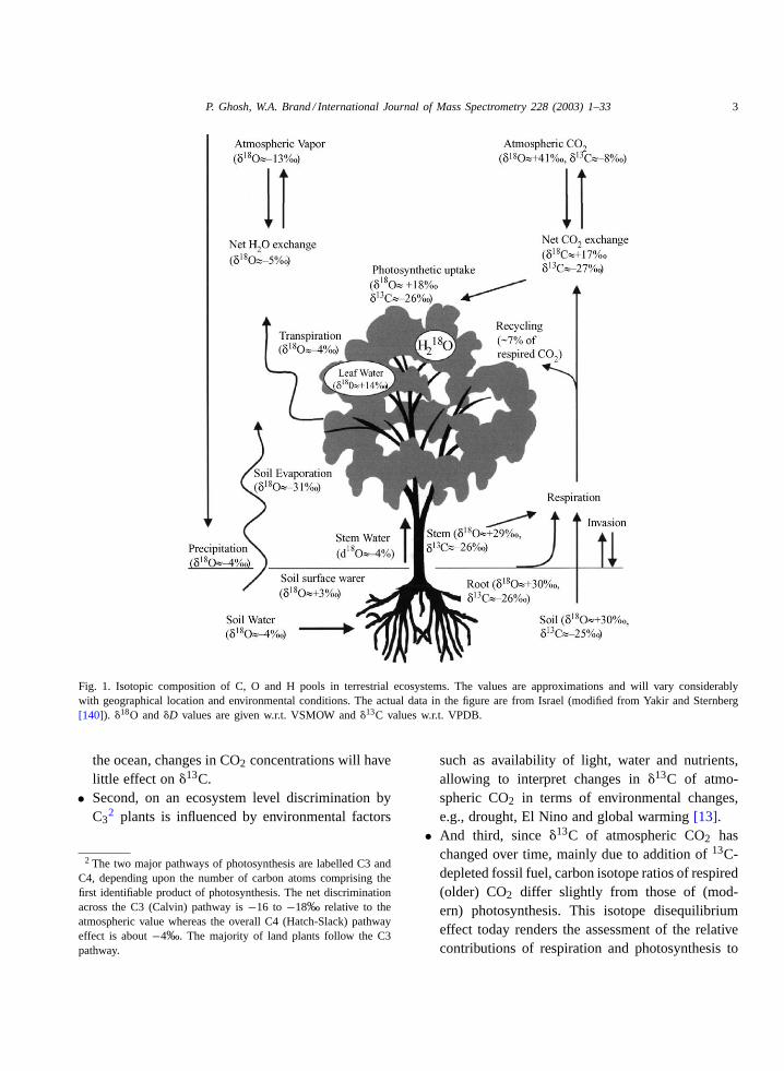
Plant photosynthesis discriminates against13C. Inother words, plant carbon tends to have less13C thanthe CO2 from which it is formed (Fig. 1). This dis-crimination provides a tool for interpreting changesin �13C1 of atmospheric CO2 which can generally beapplied in one of three ways:
• First, it can be used to partition net CO2 fluxes be-tween the land and the oceans. The known carbonbudget for the last two decades is not closed fully,hence isotope measurements can help to locate thecarbon sink missing so far as well as the processesinvolved in creating it. The missing carbon sink hasbeen postulated from budget considerations to oc-cur in the northern hemisphere[12]. This can bedone because there is little carbon isotope discrim-ination associated with exchange of CO2 betweenthe ocean and atmosphere. Consequently, if the sinkis in the land, changes in atmospheric CO2 concen-trations will be accompanied by changes in�13C,whereas if the sink is due to absorption of CO2 by
1 The carbon isotopic composition is expressed as�13C whichis defined as:�13C = {[(13C/12C)sample − (13C/12C)VPDB]/(13C/12C)VPDB} × 1000. The standard defining the13C/12C iso-tope scale is VPDB (Vienna Pee Dee Belemnite). The isotopiccomposition of CO2 gas evolved from the original PDB (carbon-ate) by reaction with phosphoric acid under specific conditions hasbeen determined by Craig[9]; by convention this gas is referredto as PDB-CO2 [10]. The original PDB material no longer exists,and its further use as an isotopic reference is discouraged[11].The VPDB scale has been introduced as a replacement[11]; it isaccessed via NBS-19, a carbonate material whose composition isdefined to be�13C = +1.95‰ and �18O = −2.2‰ relative toVPDB.
P. Ghosh, W.A. Brand / International Journal of Mass Spectrometry 228 (2003) 1–33 3
Fig. 1. Isotopic composition of C, O and H pools in terrestrial ecosystems. The values are approximations and will vary considerablywith geographical location and environmental conditions. The actual data in the figure are from Israel (modified from Yakir and Sternberg[140]). �18O and�D values are given w.r.t. VSMOW and�13C values w.r.t. VPDB.
the ocean, changes in CO2 concentrations will havelittle effect on�13C.
• Second, on an ecosystem level discrimination byC3
2 plants is influenced by environmental factors
2 The two major pathways of photosynthesis are labelled C3 andC4, depending upon the number of carbon atoms comprising thefirst identifiable product of photosynthesis. The net discriminationacross the C3 (Calvin) pathway is−16 to −18‰ relative to theatmospheric value whereas the overall C4 (Hatch-Slack) pathwayeffect is about−4‰. The majority of land plants follow the C3pathway.
such as availability of light, water and nutrients,allowing to interpret changes in�13C of atmo-spheric CO2 in terms of environmental changes,e.g., drought, El Nino and global warming[13].
• And third, since�13C of atmospheric CO2 haschanged over time, mainly due to addition of13C-depleted fossil fuel, carbon isotope ratios of respired(older) CO2 differ slightly from those of (mod-ern) photosynthesis. This isotope disequilibriumeffect today renders the assessment of the relativecontributions of respiration and photosynthesis to
4 P. Ghosh, W.A. Brand / International Journal of Mass Spectrometry 228 (2003) 1–33
changes in atmospheric CO2 difficult. On the otherhand, with improved precision in local studies, itmay help to unravel the respective signatures in thefuture.
The majority of land plants employ the C3 (seefootnote 2) photosynthetic pathway which results ina net13C depletion (∼−16 to −18‰) of the assimi-lated carbon with respect to the atmospheric value inCO2 [14]. Around 21% of modern carbon uptake byplants occurs via C4 (see footnote 2) photosynthesis,where the net discrimination against13C is smaller(∼−4‰). As a result, the global mean carbon iso-tope discrimination is slightly smaller than the pure C3
value, around−15‰ [15]. Release of CO2 from fossilfuel involves combustion of coal and petroleum, mostoriginally products of C3 photosynthesis, and whichhave been additionally modified slightly over timeby fractionation processes[16]. The isotopic compo-sition of CO2 released from fossil fuel combustion,biomass burning and soil respiration are generally sim-ilar. Hence, industrial and land use activities imposesimilar changes upon the13C/12C ratio of the globalatmosphere.
Most of the CO2 in the air–sea system is dissolvedin the oceans (>98%). Diffusion of CO2 across theair–sea interface fractionates the13C/12C ratio toabout 1/10th the degree that does terrestrial pho-tosynthesis[17]. The dissolved CO2 in general isassumed to be in isotopic equilibrium with dissolvedinorganic carbon (DIC) which contributes the bulk(∼99%) of the mixed layer carbon. At the typicalopen ocean primary production rate[18], and consid-ering time spans of centuries, marine photosynthesisglobally has minimal impact on atmospheric CO2
isotope values, mainly because any effect wouldbe diluted by DIC within the mixed layer beforereaching the atmosphere. As a consequence, atmo-spheric13C/12C records can be used to partition theuptake of fossil fuel carbon between oceanic andterrestrial reservoirs[19]. They can also be usedin studies of natural variability in the carbon cycle[20] and in calibrating global carbon budget models[21].
Fig. 1 summarises the influence of biosphericprocesses in individual compartments upon stableisotopes ratios of water and CO2. Unlike carbon, theoxygen ratio (18O/16O) of atmospheric CO2 is pri-marily determined by isotope exchange with leaf wa-ter, soil water and surface sea water[22,23]. Duringphotosynthetic gas exchange oxygen atoms are trans-ferred between carbon dioxide and leaf water withinthe cells’ chloroplasts of a photosynthesizing leaf.This equilibrium exchange reaction occurs in the pres-ence of the enzyme carbonic anhydrase, which actsas a potent catalyst for the readily reversible hydra-tion/dehydration reaction[24]. The equilibrium of theexchange reaction in this case is reached so fast that itexceeds the CO2 fixation by far and the CO2 rediffus-ing back into the atmosphere carries the leaf water18Osignal. The chloroplast water is usually enriched in18Orelative to soil water owing to evaporation from theleaves where H216O evaporates preferentially relativeto H2
18O. This relative18O enrichment of chloroplastwater (with respect to soil water) is sensitive to relativehumidity and temperature, both of which are highlyvariable in different regions of the globe. Oxygenatom exchange with soil water occurs mainly throughCO2 from soil respiration, which slowly diffuses tothe atmosphere. Oxygen atom exchange with sea wa-ter occurs through the exchange of CO2 moleculesacross the air–sea interface. The net effect of ecosys-tem specific exchange reactions can be observed in theCO2 of regional atmosphere samples when samplingis made with high spatial and temporal resolution[25].
The oxygen isotopic composition of soil andleaf water can vary considerably (−25‰ to +25‰
[26,27]). Soil water tends to follow the isotope com-position of precipitation which is progressively de-pleted in �18O relative to sea water towards highlatitudes and towards the interior of a continent. Incontrast to phenomena occurring at higher latitudes,there is no correlation between surface temperatureand �18O values of precipitation in the tropics[28].Tropical regions are characterised by converging airmasses that are forced to move vertically rather thanhorizontally. As a result they cool predominantly
P. Ghosh, W.A. Brand / International Journal of Mass Spectrometry 228 (2003) 1–33 5
by convection in atmospheric towers, while surfacetemperature gradients remain negligible. Althoughtemperature does not correlate with�18O in the trop-ics, a negative correlation has been observed betweenthe annual precipitation and�18O values at tropicalisland locations[28].
The isotopic composition of palaeo-water andpaleo-atmosphere CO2 can be obtained directly fromice core samples and trapped inclusions within icecores. Indirectly, an estimation of the isotopic com-position of past precipitation and atmosphere canalso be made from analysis of proxy records likeskeletal remains of animals, lake sediments and soilminerals that have formed in equilibrium with theirsurrounding environment.
In the following we review contemporary methodsfor determining stable isotopes relevant to climate re-search, in particular for trace gases in air, water andice, and for plant and animal organic matter. Areas ofglobal change research are discussed where isotopemeasurements have contributed significantly, includ-
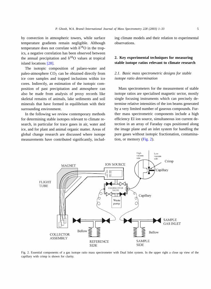
Fig. 2. Essential components of a gas isotope ratio mass spectrometer with Dual Inlet system. In the upper right a close up view of thecapillary with crimp is shown for clarity.
ing climate models and their relation to experimentalobservations.
2. Key experimental techniques for measuringstable isotope ratios relevant to climate research
2.1. Basic mass spectrometric designs for stableisotope ratio determination
Mass spectrometers for the measurement of stableisotope ratios are specialised magnetic sector, mostlysingle focusing instruments which can precisely de-termine relative intensities of the ion beams generatedby a very limited number of gaseous compounds. Fur-ther mass spectrometric components include a highefficiency EI ion source, simultaneous ion current de-tection in an array of Faraday cups positioned alongthe image plane and an inlet system for handling thepure gases without isotopic fractionation, contamina-tion, or memory (Fig. 2).
6 P. Ghosh, W.A. Brand / International Journal of Mass Spectrometry 228 (2003) 1–33
The gases in question are mainly CO2, N2, H2 andSO2. All material where isotope ratios of C, N, O, Hor S shall be determined, must be converted to one ofthese gases for measurement. Less frequently, othergases including O2, N2O, CO, SF6 and CF4 are usedfor isotopic analysis.
2.2. Inlet systems (classical Dual Inlet)
Inlet systems for gas isotope mass spectrometerscomprise valves, pipes, capillaries, connectors andgauges. Home made inlets were often made of glass,but today commercial systems prevail which aremainly designed from stainless steel. The heart of theinlet system is the change-over-valve[29], which al-lows gases from the sample and the reference side toalternately flow into the mass spectrometer. The gasesare fed from their reservoirs to the change-over-valveby capillaries of around 0.1 mm i.d. (internal diame-ter) and about 1 m in length with crimps for adjustinggas flows at their ends. Flow through both capillariesis constantly maintained, allowing one gas to enterthe mass spectrometer while the other is directed to avacuum waste pump. The smallest amount of samplethat can be analysed using such a Dual Inlet system islimited by the requirement to maintain viscous flowconditions. As a rule of thumb, the mean free path of agas molecule should not exceed 1/10th of the capillarydimensions. With the capillary dimension of 0.1 mmi.d., the lower pressure limit of viscous flow and thusaccurate measurement is about 15–20 mbar. Due tothis requirement it is necessary to concentrate the gasof interest into a small volume in front of the capillarywhen trying to reduce sample size. In conventionaloperation such volumes can be as low as 250�L. Forcondensable gases, a small cold finger can be intro-duced between reservoir and mass spectrometer inlet.This arrangement enables to measure the isotopiccomposition from∼500 nmol of sample gas.
The relative deviation in isotopic ratios betweensample and standard is expressed in theδ notation withthe δ-values commonly expressed in parts per thou-sand (per mill,‰) (see footnote 1). Primary referencescales are maintained by the IAEA Isotope Hydrology
Section[30] in Vienna. Carbon isotope ratios are re-ferred to VPDB (Vienna Pee Dee Belemnite), oxygenvalues to VPDB or VSMOW (Vienna Standard MeanOcean Water)[10,31]. Other reference scales includeVCDT (for sulfur) and atmospheric N2 (for nitrogen).VPDB is also a common reference scale for oxygenisotope ratios in the carbonate community and whenisotope ratios of CO2 in air are concerned. VSMOWalso serves as origin of the international isotope scalefor hydrogen isotopes.
2.3. Techniques for analysis of organic compounds
Organic compounds essentially comprise of carbon,nitrogen, hydrogen and oxygen. For isotopic measure-ments, CO2, N2 and H2O are generated by oxidativecombustion: [C, H, N, O] + O2 ⇒ CO2 + H2O + N2
(stoichiometry depends on the nature of the sample).Classically, the reaction is performed around 850◦Cin sealed quartz or Pyrex tubes with CuO as the oxy-gen source. Following combustion, the sealed tubesare broken one by one on a vacuum line, the prod-uct gases are released and cryogenically separated andcollected. While preparing samples for nitrogen anal-yses, CaO can be added to the quartz tube as a CO2
absorber. Before analysis, H2O is removed from thegas mixture. It can be used forD/H determination byconversion to H2. Such hydrogen gas preparation re-quires a reducing agent like uranium at a temperaturearound 800◦C [32]. Alternative reduction reagents areCr, Zn, Mn or pure C. For small samples, the producthydrogen gas can be collected on pure charcoal or canbe compressed to the required inlet pressure using aToepler pump.
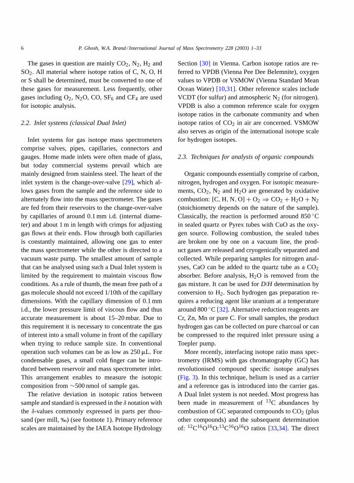
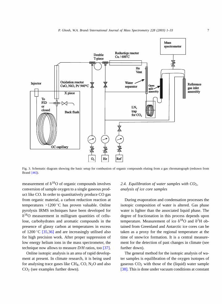
More recently, interfacing isotope ratio mass spec-trometry (IRMS) with gas chromatography (GC) hasrevolutionised compound specific isotope analyses(Fig. 3). In this technique, helium is used as a carrierand a reference gas is introduced into the carrier gas.A Dual Inlet system is not needed. Most progress hasbeen made in measurement of13C abundances bycombustion of GC separated compounds to CO2 (plusother compounds) and the subsequent determinationof: 12C16O16O:13C16O16O ratios[33,34]. The direct
P. Ghosh, W.A. Brand / International Journal of Mass Spectrometry 228 (2003) 1–33 7
Fig. 3. Schematic diagram showing the basic setup for combustion of organic compounds eluting from a gas chromatograph (redrawn fromBrand [46]).
measurement of�18O of organic compounds involvesconversion of sample oxygen to a single gaseous prod-uct like CO. In order to quantitatively produce CO gasfrom organic material, a carbon reduction reaction attemperatures >1200◦C has proven valuable. Onlinepyrolysis IRMS techniques have been developed for�18O measurement in milligram quantities of cellu-lose, carbohydrates and aromatic compounds in thepresence of glassy carbon at temperatures in excessof 1200◦C [35,36] and are increasingly utilised alsofor high precision work. After proper suppression oflow energy helium ions in the mass spectrometer, thetechnique now allows to measureD/H ratios, too[37].
Online isotopic analysis is an area of rapid develop-ment at present. In climate research, it is being usedfor analysing trace gases like CH4, CO, N2O and alsoCO2 (see examples further down).
2.4. Equilibration of water samples with CO2,analysis of ice core samples
During evaporation and condensation processes theisotopic composition of water is altered. Gas phasewater is lighter than the associated liquid phase. Thedegree of fractionation in this process depends upontemperature. Measurement of ice�18O and�2H ob-tained from Greenland and Antarctic ice cores can betaken as a proxy for the regional temperature at thetime of snow/ice formation. It is a central measure-ment for the detection of past changes in climate (seefurther down).
The general method for the isotopic analysis of wa-ter samples is equilibration of the oxygen isotopes ofgaseous CO2 with those of the (liquid) water sample[38]. This is done under vacuum conditions at constant
8 P. Ghosh, W.A. Brand / International Journal of Mass Spectrometry 228 (2003) 1–33
temperature. Using this conventional method for pale-oclimatological studies is, however, time consuming:the ice core has to be cut into small sections which areseparately packed with preparation and measurementundertaken individually for each sample. A recentlyintroduced technique[39] allows the measurement of18O/16O ratios in a continuous flow fashion: A smallblock of sample ice is firmly positioned and held on aheated device, where the ice melts continuously. Themelt water is then pumped off through a 1 cm× 1 cmbore hole in the centre of the melt head. After this,about 25% of the melt water is used for the actualmeasurement, the rest serving to seal the melted airwater mixture from ambient air. The sample wateris then loaded with CO2 in a bubble generator andisotopic equilibration is achieved at 50◦C withina long capillary. Using helium as a carrier gas theequilibrated CO2 (now carrying the18O signatureof the water sample) is liberated in a degassing sta-tion consisting of a gas permeable membrane. Theanalyte is swept through a water trap before finallyentering the IRMS via an open split for isotopicdetermination.
2.5. Isotope ratio measurements on CO2 in airsamples, key issues to ensure accuracy and precision
Global change issues have become significantdue to the sustained rise in atmospheric trace gasconcentrations (CO2, N2O, CH4) over recent years,attributable to the increased per capita energy con-sumption of a growing global population. Since theisotopic signature of these trace gases can provideinformation about the origin and fate of the gases, theability to measure their isotopic signature has becomea useful tool in the study of the nature and distributionof sources and sinks of these trace gases. Experimen-tal challenges to precisely measure isotopic ratiosof these gases arise from factors like small ambientconcentrations or small concentration differences aswell as problems with the separation and isolation ofthe required species. In particular, gas separation andisolation techniques require considerable dedication.They are extremely time-consuming given the uncer-
tainties arising from possible isotopic fractionation ineach individual step of the preparation.
One of the first air CO2 extraction systems wasdesigned at CSIRO (Aspendale) in 1982 for rou-tinely analysing air samples collected at Cape Grim(Tasmania)[40]. The Cape Grim in situ extractionline employs three high-efficiency glass U-tube trapswith internal cooling coils. At Cape Grim, a vacuumpump draws air from either a 10 or 70 m high intake,and sampling alternates between the two intakes. Airfrom the intake is dried using a cold trap at about−70◦C. CO2 is collected in a second trap immersedin liquid nitrogen. A third liquid nitrogen trap guardsagainst oil vapour back-streaming from the vacuumpump. Air flow is maintained at 300 mL min−1 for 2 h,usually during late morning when the air masses arecoming from the clean air sector. After this time, thetemperature of the trap holding the CO2 is raised to−70◦C, and the CO2 is transferred cryogenically intoa 100 mL glass flask for transport to CSIRO’s Divisionof Atmospheric Research in Aspendale. Mass spec-trometric analysis for�13C and�18O is carried out inAspendale usually within one month after collection.
In addition, whole air samples are collected in500 mL flasks. In this case, CO2 (+N2O) is cryogeni-cally separated in an automated trapping line. Thetrapping setup (Fig. 4) is based on an automated trap-ping protocol described in Allison and Francey[41].20 to 40 mL of air is allowed to pass through assem-blages of two cryotraps. All condensable material in-cluding CO2 is collected initially in the first trap. CO2(+N2O) is then slowly distilled into the second trap byraising the temperature of the first trap from−180◦Cto about −100◦C. From the second trap the CO2
is further transferred to a micro-volume cold finger.Including analysis with the mass spectrometer thewhole process takes about 15 min per flask sample.
In 1989, the stable isotope laboratory at the Insti-tute of Arctic and Alpine Research (INSTAAR, Uni-versity of Colorado) started routine measurement ofCO2 isotopes from air samples collected at the networksites operated by NOAA-CMDL (Climate Monitoringand Diagnostics Laboratory). The mass spectrometersare fitted with manifold and extraction system. The

P. Ghosh, W.A. Brand / International Journal of Mass Spectrometry 228 (2003) 1–33 9
Fig. 4. Inlet system of the MAT 252 mass spectrometer and trapping box MT Box C (Finnigan MAT, Bremen), used for analyses of CO2
from air and ice core samples at CSIRO, Aspendale (Melbourne) (redrawn from Allison and Francey[41]).
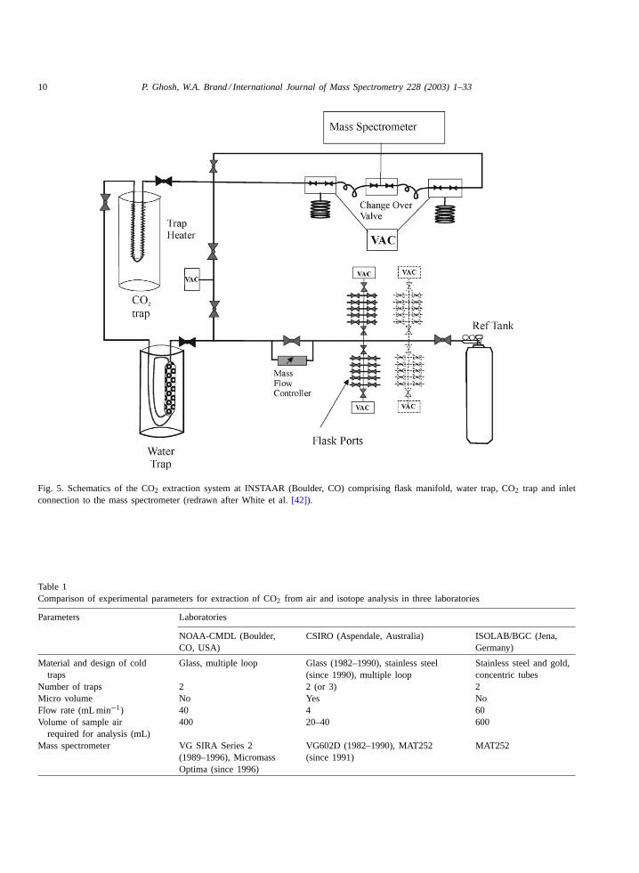
design of the extraction system differs slightly fromthe CSIRO unit (Fig. 5). The sample is diverted firstthrough a dual loop glass trap (filled with glass beads)at −70◦C followed by a CO2 trap at−196◦C. Fromhere, the analyte gas is transferred to the sample inletbellows for analysis with the mass spectrometer (fur-ther details may be found in ref.[42]).
In 1996, Trolier et al.[43] presented a 4-year timeseries of atmospheric CO2 isotope measurement fromseveral NOAA-CU sampling stations. Allison et al.[31] established a close agreement in�13C calibra-tion between NOAA and CSIRO-DAR in Australia,which allowed for the merging of the two data setsfor a two-dimensional modelling study[44]. As a con-clusion, a strong terrestrial CO2 sink operative in thenorthern mid-latitudes during 1992 and 1993 was pos-tulated.
The initially small group of laboratories has grownsteadily over the years. At the Max Planck Institutefor Biogeochemistry (Jena), we have recently devel-oped a new high precision air-CO2 extraction line forautomatic handling of air samples[45]. Like in theother laboratories, the air is sampled dry in order tomaintain the�18O signature in the flasks during trans-port and storage. The device is coupled directly to aFinnigan MAT 252 isotope ratio mass spectrometer(IRMS). Table 1gives a comparison of various param-eters used in the extraction systems at NOAA-CMDL,CSIRO-DAR and MPI-BGC.
2.5.1. N2O correctionSeparating the relative ion current contributions of
CO2•+ and N2O•+ in isotopic measurement is essen-
tial as both of them have nearly identical molecular
10 P. Ghosh, W.A. Brand / International Journal of Mass Spectrometry 228 (2003) 1–33
Fig. 5. Schematics of the CO2 extraction system at INSTAAR (Boulder, CO) comprising flask manifold, water trap, CO2 trap and inletconnection to the mass spectrometer (redrawn after White et al.[42]).
Table 1Comparison of experimental parameters for extraction of CO2 from air and isotope analysis in three laboratories
Parameters Laboratories
NOAA-CMDL (Boulder,CO, USA)
CSIRO (Aspendale, Australia) ISOLAB/BGC (Jena,Germany)
Material and design of coldtraps
Glass, multiple loop Glass (1982–1990), stainless steel(since 1990), multiple loop
Stainless steel and gold,concentric tubes
Number of traps 2 2 (or 3) 2Micro volume No Yes NoFlow rate (mL min−1) 40 4 60Volume of sample air
required for analysis (mL)400 20–40 600
Mass spectrometer VG SIRA Series 2(1989–1996), MicromassOptima (since 1996)
VG602D (1982–1990), MAT252(since 1991)
MAT252
P. Ghosh, W.A. Brand / International Journal of Mass Spectrometry 228 (2003) 1–33 11
weight and the mass spectrometer cannot distinguishbetween them (complete separation of the isobaricions would require a working resolution in excess of5000 for the three ion currents including high qualityabundance sensitivity properties of the MS). If one isinterested in the�15N of �18O of N2O, separation of(neutral) CO2 from N2O may be done by absorbingCO2 onto soda lime and collect the remaining N2Ofor isotopic measurement. For analysis of�13C and�18O in CO2, a separation procedure is a little morecomplex. It can be accomplished in three ways:
• Separate determination or measurement of the rela-tive contributions and removal of N2O•+ from theCO2 signal using a mass balance correction.
• Physical removal of N2O from CO2 by convertingN2O to N2 prior to measurement. This is achievedby passing the sample gas through a reducing agent(copper at 500◦C).
• Physical separation of CO2 and N2O using a gaschromatograph coupled online to an isotope ratiomass spectrometer.
The mass balance correction depends on a precisedetermination of the relative mixing ratios of the gases.The reducing agent approach can cause fractionationof the18O/16O signature during the high temperaturechemical reaction. The third approach of using a gaschromatograph for separating CO2 from N2O occurswithout isotopic alteration[34,46]. This technique iscapable of generating reproducible results with a pre-cision of 0.05 and 0.08‰, respectively for carbon andoxygen isotopes in case of air CO2 (which often is notsufficient for data interpretation). For reasons of pre-cision, most laboratories routinely measuring the iso-topic composition of CO2 in air samples remove theN2O•+ contribution to the CO2•+ ion currents[47,48]using the mass balance correction approach. Possibleisotopic variations in N2O have little influence and areneglected in this case.
2.5.2. Analysis of air trapped in ice coresFor obtaining an ice core trace gas concentration and
isotopic record, trapped air must be released from theice sample, thereby carefully maintaining the quantita-
tive composition. The ice is either molten for completetrace gas extraction (suitable for most trace gases, butnot for CO2) or it is mechanically crushed or groundat −20◦C under vacuum[49,50]. The air escapingfrom the bubbles is then collected by condensationat 14 K. Because not all bubbles are opened, extrac-tion efficiency for the crushing technique is generallyonly 80–90%. After crushing, a small amount of theevolved gas is used for gas chromatographic determi-nation. For CO2 concentration the measurement pre-cision is approximately 3 ppm. The major part of thesample gas is used for isotopic analysis. Here, CO2 (to-gether with N2O) is quantitatively separated from theremainder of the sample at−196◦C in a metal vacuumline. The results are corrected for the isobaric inter-ference of N2O. Accuracy of the�13C results is about0.1‰, as determined by analysing artificial CO2 in airmixtures and from the scatter of the results aroundthe smooth line. In order to increase the resolution of�13C records attempts are made to lower the amountof ice consumed without compromising precision.
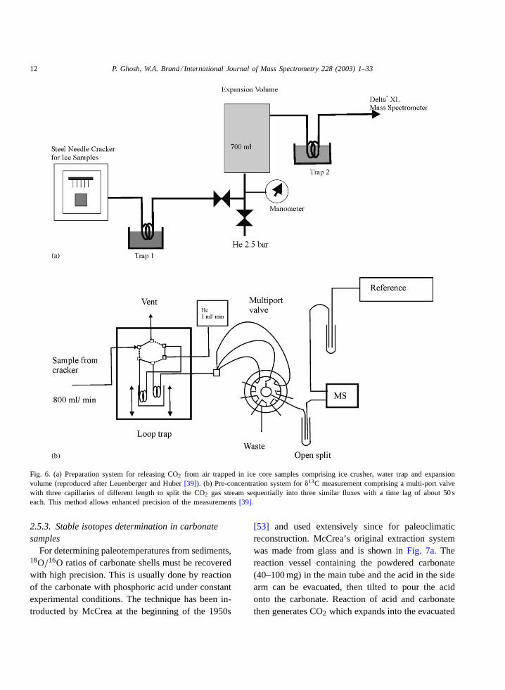
Conventional offline techniques require relativelylarge amounts of ice. A new combined technique ofgas chromatography and mass spectrometry has re-cently been introduced[51] which allows to work withdrastically reduced sample amounts. The correspond-ing 5–10 g of ice contain only 0.5–1 mL S.T.P. of airor 0.1–0.2�L of CO2. The main components of thesystem are shown inFig. 6a. In short, a stainless steelneedle cracker is connected online with an isotope ra-tio mass spectrometer. Cracking of ice is done around−30◦C. From the cracker the gas expands through awater trap (−70◦C) into a larger stainless steel con-tainer (700 mL) from where it is flushed out with he-lium for isotopic analysis using a modified FinniganMAT Precon system[52] (Fig. 6b). CO2 is removedfrom the carrier gas in a small trap and frozen onto thecolumn head prior to low flow (2 mL min−1) gas chro-matographic separation and online isotopic analysis.Correction for N2O is not necessary in this case dueto the separation of the two gases on the GC-column.Accuracy of the�13C results is about 0.1‰, as deter-mined by analysing artificial CO2 in air mixtures andfrom the scatter of the results around the smooth line.
12 P. Ghosh, W.A. Brand / International Journal of Mass Spectrometry 228 (2003) 1–33
Fig. 6. (a) Preparation system for releasing CO2 from air trapped in ice core samples comprising ice crusher, water trap and expansionvolume (reproduced after Leuenberger and Huber[39]). (b) Pre-concentration system for�13C measurement comprising a multi-port valvewith three capillaries of different length to split the CO2 gas stream sequentially into three similar fluxes with a time lag of about 50 seach. This method allows enhanced precision of the measurements[39].
2.5.3. Stable isotopes determination in carbonatesamples
For determining paleotemperatures from sediments,18O/16O ratios of carbonate shells must be recoveredwith high precision. This is usually done by reactionof the carbonate with phosphoric acid under constantexperimental conditions. The technique has been in-troducted by McCrea at the beginning of the 1950s
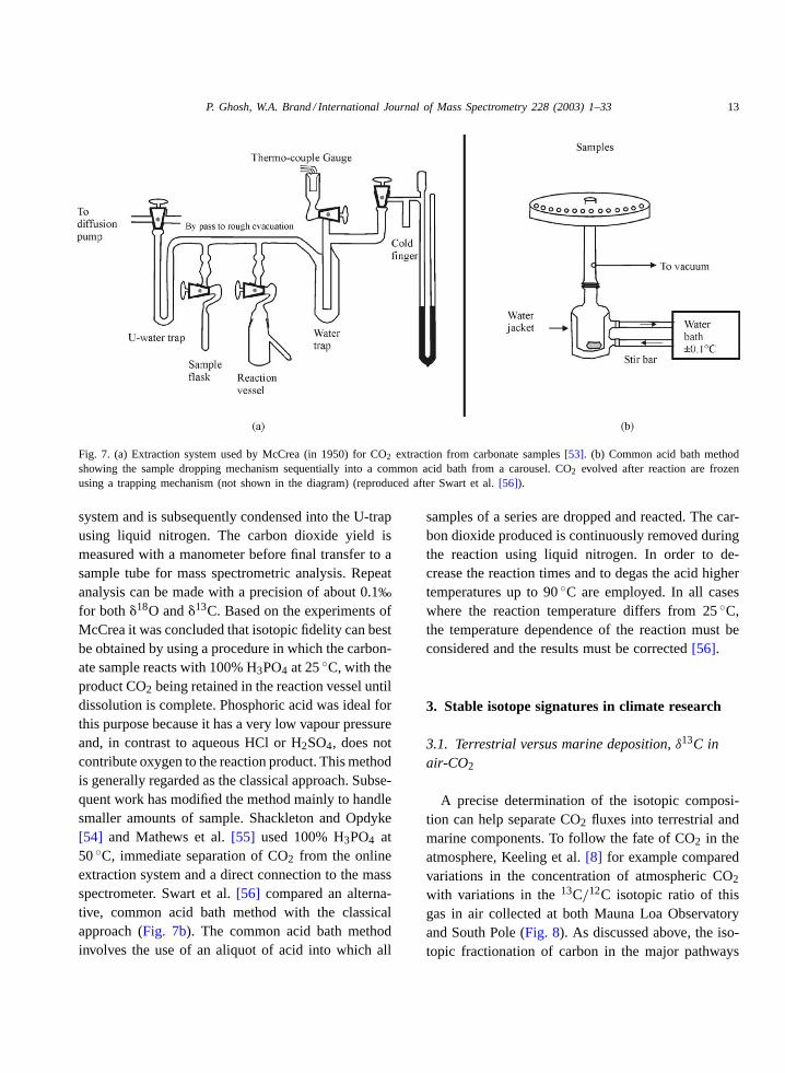
[53] and used extensively since for paleoclimaticreconstruction. McCrea’s original extraction systemwas made from glass and is shown inFig. 7a. Thereaction vessel containing the powdered carbonate(40–100 mg) in the main tube and the acid in the sidearm can be evacuated, then tilted to pour the acidonto the carbonate. Reaction of acid and carbonatethen generates CO2 which expands into the evacuated
P. Ghosh, W.A. Brand / International Journal of Mass Spectrometry 228 (2003) 1–33 13
Fig. 7. (a) Extraction system used by McCrea (in 1950) for CO2 extraction from carbonate samples[53]. (b) Common acid bath methodshowing the sample dropping mechanism sequentially into a common acid bath from a carousel. CO2 evolved after reaction are frozenusing a trapping mechanism (not shown in the diagram) (reproduced after Swart et al.[56]).
system and is subsequently condensed into the U-trapusing liquid nitrogen. The carbon dioxide yield ismeasured with a manometer before final transfer to asample tube for mass spectrometric analysis. Repeatanalysis can be made with a precision of about 0.1‰
for both�18O and�13C. Based on the experiments ofMcCrea it was concluded that isotopic fidelity can bestbe obtained by using a procedure in which the carbon-ate sample reacts with 100% H3PO4 at 25◦C, with theproduct CO2 being retained in the reaction vessel untildissolution is complete. Phosphoric acid was ideal forthis purpose because it has a very low vapour pressureand, in contrast to aqueous HCl or H2SO4, does notcontribute oxygen to the reaction product. This methodis generally regarded as the classical approach. Subse-quent work has modified the method mainly to handlesmaller amounts of sample. Shackleton and Opdyke[54] and Mathews et al.[55] used 100% H3PO4 at50◦C, immediate separation of CO2 from the onlineextraction system and a direct connection to the massspectrometer. Swart et al.[56] compared an alterna-tive, common acid bath method with the classicalapproach (Fig. 7b). The common acid bath methodinvolves the use of an aliquot of acid into which all
samples of a series are dropped and reacted. The car-bon dioxide produced is continuously removed duringthe reaction using liquid nitrogen. In order to de-crease the reaction times and to degas the acid highertemperatures up to 90◦C are employed. In all caseswhere the reaction temperature differs from 25◦C,the temperature dependence of the reaction must beconsidered and the results must be corrected[56].
3. Stable isotope signatures in climate research
3.1. Terrestrial versus marine deposition, δ13C inair-CO2
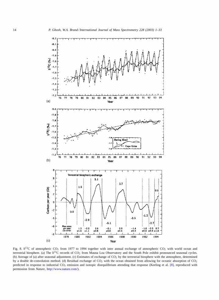
A precise determination of the isotopic composi-tion can help separate CO2 fluxes into terrestrial andmarine components. To follow the fate of CO2 in theatmosphere, Keeling et al.[8] for example comparedvariations in the concentration of atmospheric CO2
with variations in the13C/12C isotopic ratio of thisgas in air collected at both Mauna Loa Observatoryand South Pole (Fig. 8). As discussed above, the iso-topic fractionation of carbon in the major pathways
14 P. Ghosh, W.A. Brand / International Journal of Mass Spectrometry 228 (2003) 1–33
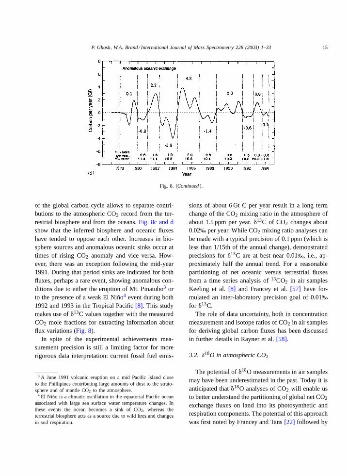
Fig. 8. �13C of atmospheric CO2 from 1977 to 1994 together with inter annual exchange of atmospheric CO2 with world ocean andterrestrial biosphere. (a) The�13C records of CO2 from Mauna Loa Observatory and the South Pole exhibit pronounced seasonal cycles.(b) Average of (a) after seasonal adjustment. (c) Estimates of exchange of CO2 by the terrestrial biosphere with the atmosphere, determinedby a double de-convolution method. (d) Residual exchange of CO2 with the ocean obtained from allowing for oceanic absorption of CO2
predicted in response to industrial CO2 emission and isotopic disequilibrium attending that response (Keeling et al.[8], reproduced withpermission fromNature, http://www.nature.com/).
P. Ghosh, W.A. Brand / International Journal of Mass Spectrometry 228 (2003) 1–33 15
Fig. 8. (Continued ).
of the global carbon cycle allows to separate contri-butions to the atmospheric CO2 record from the ter-restrial biosphere and from the oceans.Fig. 8c and dshow that the inferred biosphere and oceanic fluxeshave tended to oppose each other. Increases in bio-sphere sources and anomalous oceanic sinks occur attimes of rising CO2 anomaly and vice versa. How-ever, there was an exception following the mid-year1991. During that period sinks are indicated for bothfluxes, perhaps a rare event, showing anomalous con-ditions due to either the eruption of Mt. Pinatubo3 orto the presence of a weak El Niño4 event during both1992 and 1993 in the Tropical Pacific[8]. This studymakes use of�13C values together with the measuredCO2 mole fractions for extracting information aboutflux variations (Fig. 8).
In spite of the experimental achievements mea-surement precision is still a limiting factor for morerigorous data interpretation: current fossil fuel emis-
3 A June 1991 volcanic eruption on a mid Pacific Island closeto the Phillipines contributing large amounts of dust to the strato-sphere and of mantle CO2 to the atmosphere.
4 El Niño is a climatic oscillation in the equatorial Pacific oceanassociated with large sea surface water temperature changes. Inthese events the ocean becomes a sink of CO2, whereas theterrestrial biosphere acts as a source due to wild fires and changesin soil respiration.
sions of about 6 Gt C per year result in a long termchange of the CO2 mixing ratio in the atmosphere ofabout 1.5 ppm per year.�13C of CO2 changes about0.02‰ per year. While CO2 mixing ratio analyses canbe made with a typical precision of 0.1 ppm (which isless than 1/15th of the annual change), demonstratedprecisions for�13C are at best near 0.01‰, i.e., ap-proximately half the annual trend. For a reasonablepartitioning of net oceanic versus terrestrial fluxesfrom a time series analysis of13CO2 in air samplesKeeling et al.[8] and Francey et al.[57] have for-mulated an inter-laboratory precision goal of 0.01‰
for �13C.The role of data uncertainty, both in concentration
measurement and isotope ratios of CO2 in air samplesfor deriving global carbon fluxes has been discussedin further details in Rayner et al.[58].
3.2. δ18O in atmospheric CO2
The potential of�18O measurements in air samplesmay have been underestimated in the past. Today it isanticipated that�18O analyses of CO2 will enable usto better understand the partitioning of global net CO2
exchange fluxes on land into its photosynthetic andrespiration components. The potential of this approachwas first noted by Francey and Tans[22] followed by
16 P. Ghosh, W.A. Brand / International Journal of Mass Spectrometry 228 (2003) 1–33
more rigorous investigations showing an appreciable�18O signal (latitudinal gradients and seasonal varia-tions) connected to biospheric activity in the globalatmosphere as well as consistency in the global scale18O mass balance[22,59–61]. These studies also re-iterated the critical need to reduce the uncertaintyassociated with oxygen isotope measurements. Inorder to extract a maximum of information, high pre-cision and accuracy in determining�13C and �18Ovalues over decadal or greater timescales is important.Only a handful of laboratories have to date demon-strated an ability to measure�13C from CO2 in airwith long term precision of 0.015‰. Inter-laboratoryprecision in case of oxygen is still poor com-pared to an expected target precision of 0.03‰ in�18O [62].
3.3. Paleoclimate reconstruction
While it has been possible for the past 50 years tomeasure the CO2 mixing ratio and the isotopic compo-sition of air samples directly, this information must berecovered by more indirect means for the more distantpast. Much of our quantitative knowledge of climatefluctuation in the past has been derived from recordspreserved in ice sheets and deep sea sediments.
The main palaeoclimatic indicators have been theabundance ratios of the oxygen isotopes in water aswell as oxygen and carbon isotopes in carbonates.The difference in physical properties caused by themass difference leads to temperature dependent iso-topic fractionations during phase changes and chem-ical reactions. This allows the oxygen isotopic ratioto be used as a tracer for studying: (1) climate andthe hydrological cycle, (2) carbonate precipitation anddissolution and (3) photosynthesis and related process.Products formed as a result of interaction between wa-ter and its surrounding can be preserved over timeand can, with the isotopic signature, serve as a proxyrecord of past climate change.
Different types of palaeoclimatic records from icesheets and ice caps, peat bogs, lake and ocean sedi-ments, loess deposits, speleothems and tree rings fromdifferent parts of the world provide a mosaic of well
documented local responses to global climate changes.But for a meaningful comparison it is essential that thetiming of the different records is accurately known andthat differences in response time for different recordsare considered during interpretation.
3.3.1. Water and air trapped in ice coresThe water oxygen and hydrogen isotopic composi-
tion of ice cores have preserved palaeoclimatic infor-mation such as local temperatures and precipitationrate, moisture source conditions, etc., whereas trappedair within ice cores directly provides atmospherictrace gas concentrations and indirectly allows to es-timate aerosol fluxes of marine, volcanic, terrestrial,cosmogenic and anthropogenic origin[50,57,63]. Theice-drilling project undertaken in the framework of along term collaboration between Russia, the US andFrance at the Russian Vostok Station in East Antarc-tica has provided a wealth of information of changesin climate and atmospheric trace gas and aerosol com-position over the past four glacial–interglacial cycles(i.e., for the last 400,000 years[64]).
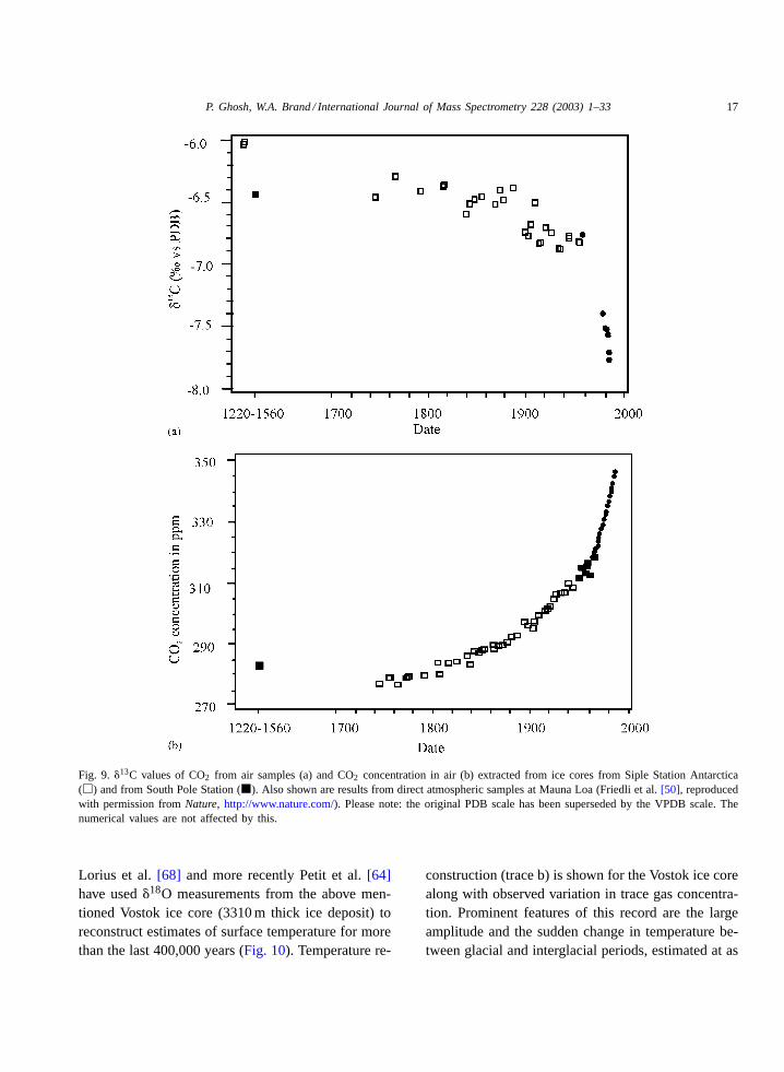
The data plotted inFig. 9a and bshow�13C resultsobtained from trapped air in an Antarctic ice core[50]. It represents one of the earliest results from icecores exhibiting a general increase in CO2 concentra-tion with time since 1750 together with a decrease in�13C values. Using these data it was possible to di-rectly compare measurements of CO2 concentrationsin air obtained at Mauna Loa since 1958 by Keel-ing et al. [8] with the longer term ice core archiverecord from Antarctica. The average�13C value ofsamples before 1800 A.D. is−6.41‰ in the ice core.This observation is in excellent agreement with theextrapolated pre-industrial mean value for the SouthPole inferred from direct air sampling (−6.44‰) andtherefore adds confidence to using ice cores as a toolfor palaeoclimatic investigations.
Continuous ice cores for studying past climaticevents are also available from Greenland or alpineglaciers[65]. Dansgaard et al.[66] and Johnsen et al.[67] have utilised oxygen isotope measurements inice cores from Greenland to reconstruct surface tem-perature exceeding the last 100,000 years. Similarly,
P. Ghosh, W.A. Brand / International Journal of Mass Spectrometry 228 (2003) 1–33 17
Fig. 9. �13C values of CO2 from air samples (a) and CO2 concentration in air (b) extracted from ice cores from Siple Station Antarctica(�) and from South Pole Station (�). Also shown are results from direct atmospheric samples at Mauna Loa (Friedli et al.[50], reproducedwith permission fromNature, http://www.nature.com/). Please note: the original PDB scale has been superseded by the VPDB scale. Thenumerical values are not affected by this.
Lorius et al.[68] and more recently Petit et al.[64]have used�18O measurements from the above men-tioned Vostok ice core (3310 m thick ice deposit) toreconstruct estimates of surface temperature for morethan the last 400,000 years (Fig. 10). Temperature re-
construction (trace b) is shown for the Vostok ice corealong with observed variation in trace gas concentra-tion. Prominent features of this record are the largeamplitude and the sudden change in temperature be-tween glacial and interglacial periods, estimated at as
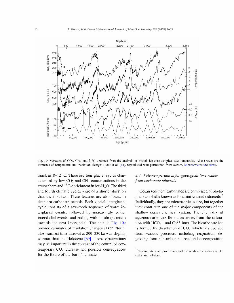
18 P. Ghosh, W.A. Brand / International Journal of Mass Spectrometry 228 (2003) 1–33
P. Ghosh, W.A. Brand / International Journal of Mass Spectrometry 228 (2003) 1–33 19
of dead organic matter. The calcium ion mainly orig-inates from weathering of the continental platform.The microscopic animals secret a shell around theirbody as a protective covering, thereby effectively de-creasing the concentration of HCO3
− and Ca2+ ionsin the surrounding water. After death the animal shellssink down to the ocean floor and remain preservedin sediments. The shells are made up of two types ofcarbonate mineral; calcite and its precursor aragonite.Calcite and aragonite are enriched in18O comparedto the water from which they were precipitated. Whenthe reaction takes place in isotopic equilibrium, the�18O value of the calcite can be related to�18O ofsea water and the temperature (in◦C) by [53,70]:
T = 16.9 − 4.2(δc − δw) + 0.13(δc − δw)2
whereδc is the�18O value of CO2 prepared by reactingcalcite with 100% H3PO4 at 25◦C andδw is �18O ofCO2 in equilibrium with water at 25◦C. Bothδ-valuesare on the same (VSMOW) scale.
The oxygen isotopic palaeo-thermometer is basedon the assumption that biogenic calcite and arago-nite are precipitated in isotopic equilibrium with seawater. This requirement is met only by a few car-bonate secreting organisms including molluscs andforaminifera. For shells from these organisms, for ev-ery 1◦C rise in water temperature there is 0.25‰ dropin �18O of carbonate in isotopic equilibrium with thatwater. Decreasing�18O values in shell carbonate thusindicate increasing temperatures if�18O of the waterwere to have remained constant. This is obviously notalways the case, especially during glacial/interglacialperiods because of the large effect of ice piling up inthe polar areas. More information is needed to decou-ple the�18O source from the temperature signal. Insome cases this conflict can be resolved by simultane-ous measurement of trace elemental ratios like Sr/Ca.For corals, such ratios are independent of salinitywhich reflects the source water oxygen isotopic com-position. Hence, for coral cores found in proximity tothe cores used for paleotemperature determination, acorrection is possible and unambiguous temperaturescan be derived[71].
The carbon isotopic composition (�13C) is deter-mined by CO2 forming the HCO3
− ion. The sourceof CO2 is mainly respiration and decomposition oforganic matter. Both these processes produce CO2
of similar isotopic signature. In phytoplankton car-bon isotopic composition is predominantly controlledby photosynthetic activity. Other factors like temper-ature are of minor significance. Therefore, variationsof �18O and�13C in marine planktonic foraminiferacan potentially be used to understand the variabilityof photosynthetic activity in the past.
Despite the potentially complex array of controls,natural waters tend to show a characteristic range ofcarbon and oxygen isotope values which in turn aremimicked or tracked by the carbonate minerals precip-itated from them. Consequently, plots of�18O versus�13C for carbonate materials can help identify theirdepositional and/or diagenetic environment(s). Usingstable isotope analysis of carbonates enables us tostudy the conditions of deposition and to estimate thetemperature of formation[53].
3.5. The deep sea stable isotope record
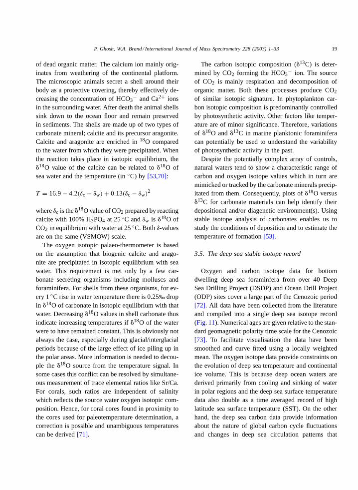
Oxygen and carbon isotope data for bottomdwelling deep sea foraminfera from over 40 DeepSea Drilling Project (DSDP) and Ocean Drill Project(ODP) sites cover a large part of the Cenozoic period[72]. All data have been collected from the literatureand compiled into a single deep sea isotope record(Fig. 11). Numerical ages are given relative to the stan-dard geomagnetic polarity time scale for the Cenozoic[73]. To facilitate visualisation the data have beensmoothed and curve fitted using a locally weightedmean. The oxygen isotope data provide constraints onthe evolution of deep sea temperature and continentalice volume. This is because deep ocean waters arederived primarily from cooling and sinking of waterin polar regions and the deep sea surface temperaturedata also double as a time averaged record of highlatitude sea surface temperature (SST). On the otherhand, the deep sea carbon data provide informationabout the nature of global carbon cycle fluctuationsand changes in deep sea circulation patterns that
20 P. Ghosh, W.A. Brand / International Journal of Mass Spectrometry 228 (2003) 1–33
Fig. 11. Global deep sea oxygen and carbon isotope records based on data for more than 40 Deep Sea Drilling Project and Ocean DrillingProject sites (Zachos et al.[72], reproduced with permission fromScience Magazine, http://www.sciencemag.org/). Some key tectonic andbiotic events are marked in the diagram. (*) The temperature scale has been inferred from the�18O record assuming an ice-free oceanwith �18O∼12‰ w.r.t. VSMOW [72].
might produce or arise from climatic changes. The�18O and�13C records inFig. 11demonstrate severalmajor and some minor episodes of climatic changesduring last 70 Ma. The sudden drop in isotopic ra-tios (both for carbon and oxygen isotopes) denoteseffects caused by warming processes. These episodesare denoted by arrows indicating geological periodswith high ocean temperature. Many of these trendsare tectonically controlled and reflect sudden input ofhydrothermal fluids from deep inside the Earth. Theimpact of the Earth’s tectonic activity caused ma-
jor shifts in climate and played an important role inproviding conducive conditions for biotic evolution.
The marine carbon isotopic composition was con-sidered an invariant quantity (∼0‰ w.r.t. VPDB) un-til 1980 when it was realised that oscillating secularsignals are preserved in stratigraphic records[74–77]marking the times of major global changes in Earth’shistory. In contrast to the below-discussed oxygen iso-topes, the pristine nature of this�13C carbonate secu-lar trend has not been criticised. Diagenetic alterationof carbonates occurs in a system with a low water/rock
P. Ghosh, W.A. Brand / International Journal of Mass Spectrometry 228 (2003) 1–33 21
ratio for carbon, and a high ratio for oxygen[78,79].Diagenetic stabilisation of carbonates therefore resultsin transport of carbon from a precursor to a succes-sor mineral phase. Oscillations in the�13C carbonatetrend can thus be utilised for correlation and isotopestratigraphy[80,81]. This proxy, however, is subjectto several limitations as compared to Sr isotopes. Themajor difference arises from the fact that�13C of oceancarbonate at any given time can show a considerablespread of values due to spatial variability of oceanic�13C [82] and due to biological factors present dur-ing shell formation[83]. The complications arise notso much during logging of a single well or a profile,but can become considerable when isolated sedimen-tary sequences or wells are compared. Nonetheless,large peaks can serve as correlation markers, particu-larly in the Precambrian[84]. In addition, the secular�13C carbonate trend can be used as an indicator for
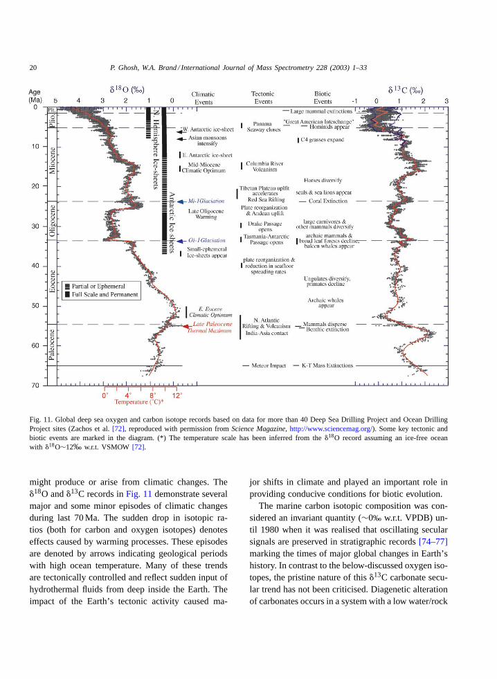
Fig. 12. Phanerozoic�13C trend of the world ocean. The running mean is based on 20 Ma windows and 5 Ma forward step. The shadedarea around the running mean includes 68 and 95% of all data, respectively (modified after Veizer et al.[87]). See also note in the captionto Fig. 9.
determining oceanic palaeo-productivity and preserva-tion patterns, ancientpCO2 andpO2 states, and simi-lar palaeo-environmental phenomena[85–87]. Fig. 12,shows combined�13C data from limestone and shellportions plotted against age as compiled in Veizer et al.[87]. This plot shows the secular variation as an in-crease in�13C throughout the Paleozoic, followed byan abrupt decline and subsequent oscillations aroundthe present-day value in the course of the Mesozoicand Cenozoic. This variation can be compared withSr isotope ratio variations during the Phanerozoic.The running mean based on these values was calcu-lated for 5 Ma incremental shifts[87] to make it use-ful for global bio-stratigraphic correlation. The bandsaround this mean incorporate 68 and 95% of all mea-sured samples, respectively. Considering the globalnature of the data set, with samples originating fromfive continents and a multitude of sedimentary basins,
22 P. Ghosh, W.A. Brand / International Journal of Mass Spectrometry 228 (2003) 1–33
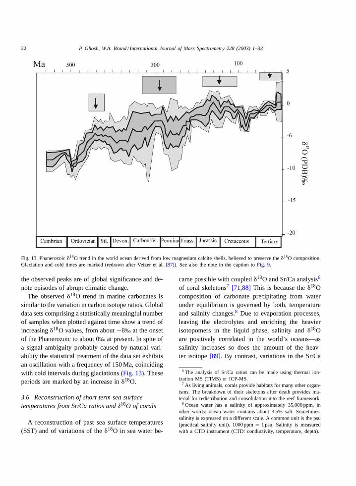
Fig. 13. Phanerozoic�18O trend in the world ocean derived from low magnesium calcite shells, believed to preserve the�18O composition.Glaciation and cold times are marked (redrawn after Veizer et al.[87]). See also the note in the caption toFig. 9.
the observed peaks are of global significance and de-note episodes of abrupt climatic change.
The observed�18O trend in marine carbonates issimilar to the variation in carbon isotope ratios. Globaldata sets comprising a statistically meaningful numberof samples when plotted against time show a trend ofincreasing�18O values, from about−8‰ at the onsetof the Phanerozoic to about 0‰ at present. In spite ofa signal ambiguity probably caused by natural vari-ability the statistical treatment of the data set exhibitsan oscillation with a frequency of 150 Ma, coincidingwith cold intervals during glaciations (Fig. 13). Theseperiods are marked by an increase in�18O.
3.6. Reconstruction of short term sea surfacetemperatures from Sr/Ca ratios and δ18O of corals
A reconstruction of past sea surface temperatures(SST) and of variations of the�18O in sea water be-
came possible with coupled�18O and Sr/Ca analysis6
of coral skeletons7 [71,88] This is because the�18Ocomposition of carbonate precipitating from waterunder equilibrium is governed by both, temperatureand salinity changes.8 Due to evaporation processes,leaving the electrolytes and enriching the heavierisotopomers in the liquid phase, salinity and�18Oare positively correlated in the world’s oceans—assalinity increases so does the amount of the heav-ier isotope[89]. By contrast, variations in the Sr/Ca
6 The analysis of Sr/Ca ratios can be made using thermal ion-ization MS (TIMS) or ICP-MS.
7 As living animals, corals provide habitats for many other organ-isms. The breakdown of their skeletons after death provides ma-terial for redistribution and consolidation into the reef framework.
8 Ocean water has a salinity of approximately 35,000 ppm, inother words: ocean water contains about 3.5% salt. Sometimes,salinity is expressed on a different scale. A common unit is the psu(practical salinity unit). 1000 ppm= 1 psu. Salinity is measuredwith a CTD instrument (CTD: conductivity, temperature, depth).
P. Ghosh, W.A. Brand / International Journal of Mass Spectrometry 228 (2003) 1–33 23
ratio of coral carbonate are independent of salinitychanges. Therefore, combining�18O and Sr/Ca ratiosallows the determination of past changes in sea-water�18O composition, which is useful to study variationsin tropical hydrological cycles. The change in sea wa-ter �18O is defined by the differences between coralSr/Ca and�18O curves (residual�18O). Differences insea water�18O should reflect changes in sea surfacesalinity (SSS) because rainfall on land is depleted in18O relative to sea water, while evaporation tends toenrich the surface ocean in18O [90].
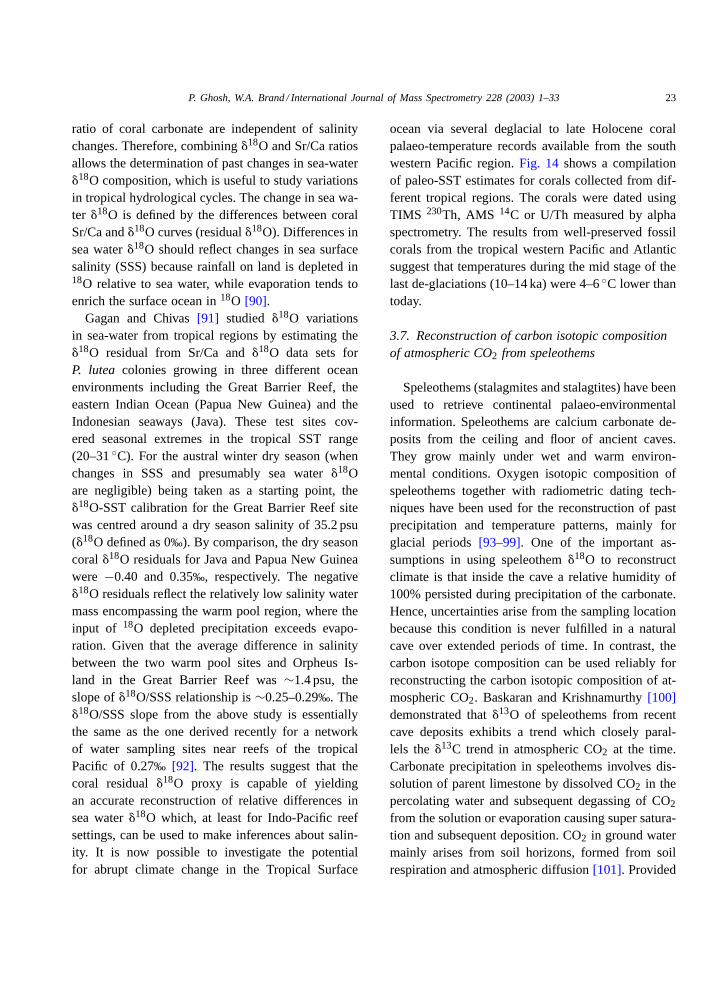
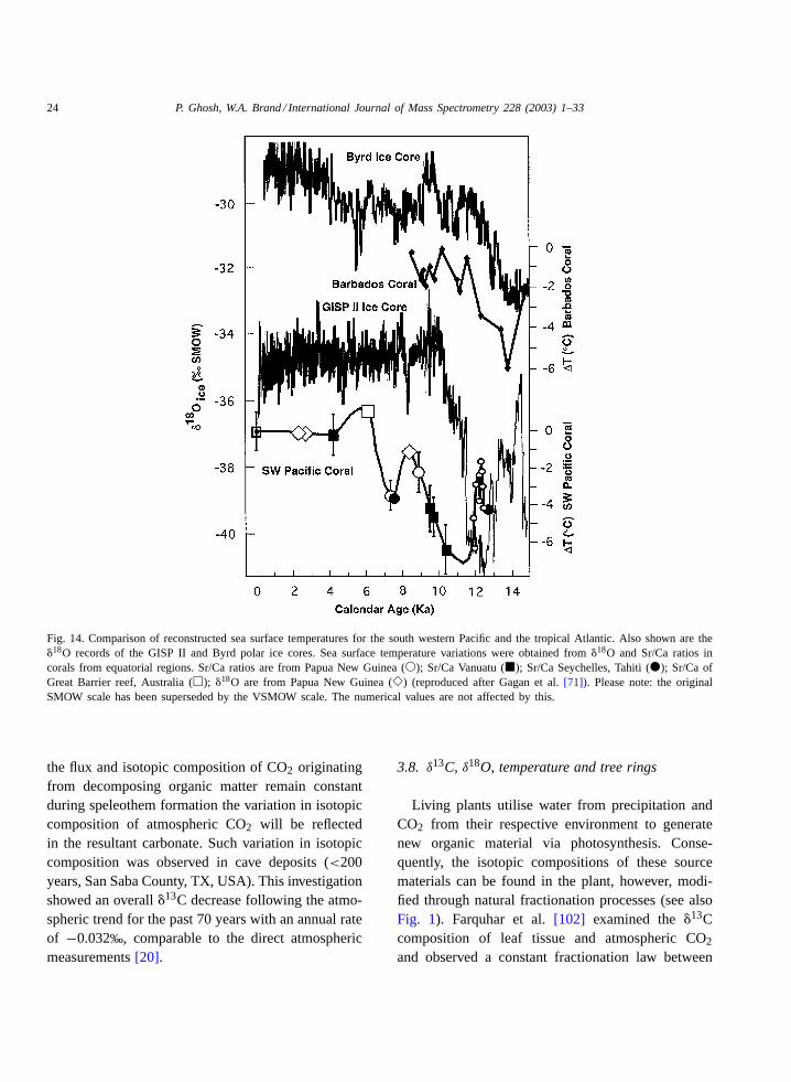
Gagan and Chivas[91] studied �18O variationsin sea-water from tropical regions by estimating the�18O residual from Sr/Ca and�18O data sets forP. lutea colonies growing in three different oceanenvironments including the Great Barrier Reef, theeastern Indian Ocean (Papua New Guinea) and theIndonesian seaways (Java). These test sites cov-ered seasonal extremes in the tropical SST range(20–31◦C). For the austral winter dry season (whenchanges in SSS and presumably sea water�18Oare negligible) being taken as a starting point, the�18O-SST calibration for the Great Barrier Reef sitewas centred around a dry season salinity of 35.2 psu(�18O defined as 0‰). By comparison, the dry seasoncoral �18O residuals for Java and Papua New Guineawere −0.40 and 0.35‰, respectively. The negative�18O residuals reflect the relatively low salinity watermass encompassing the warm pool region, where theinput of 18O depleted precipitation exceeds evapo-ration. Given that the average difference in salinitybetween the two warm pool sites and Orpheus Is-land in the Great Barrier Reef was∼1.4 psu, theslope of�18O/SSS relationship is∼0.25–0.29‰. The�18O/SSS slope from the above study is essentiallythe same as the one derived recently for a networkof water sampling sites near reefs of the tropicalPacific of 0.27‰ [92]. The results suggest that thecoral residual�18O proxy is capable of yieldingan accurate reconstruction of relative differences insea water�18O which, at least for Indo-Pacific reefsettings, can be used to make inferences about salin-ity. It is now possible to investigate the potentialfor abrupt climate change in the Tropical Surface
ocean via several deglacial to late Holocene coralpalaeo-temperature records available from the southwestern Pacific region.Fig. 14 shows a compilationof paleo-SST estimates for corals collected from dif-ferent tropical regions. The corals were dated usingTIMS 230Th, AMS 14C or U/Th measured by alphaspectrometry. The results from well-preserved fossilcorals from the tropical western Pacific and Atlanticsuggest that temperatures during the mid stage of thelast de-glaciations (10–14 ka) were 4–6◦C lower thantoday.
3.7. Reconstruction of carbon isotopic compositionof atmospheric CO2 from speleothems
Speleothems (stalagmites and stalagtites) have beenused to retrieve continental palaeo-environmentalinformation. Speleothems are calcium carbonate de-posits from the ceiling and floor of ancient caves.They grow mainly under wet and warm environ-mental conditions. Oxygen isotopic composition ofspeleothems together with radiometric dating tech-niques have been used for the reconstruction of pastprecipitation and temperature patterns, mainly forglacial periods[93–99]. One of the important as-sumptions in using speleothem�18O to reconstructclimate is that inside the cave a relative humidity of100% persisted during precipitation of the carbonate.Hence, uncertainties arise from the sampling locationbecause this condition is never fulfilled in a naturalcave over extended periods of time. In contrast, thecarbon isotope composition can be used reliably forreconstructing the carbon isotopic composition of at-mospheric CO2. Baskaran and Krishnamurthy[100]demonstrated that�13O of speleothems from recentcave deposits exhibits a trend which closely paral-lels the�13C trend in atmospheric CO2 at the time.Carbonate precipitation in speleothems involves dis-solution of parent limestone by dissolved CO2 in thepercolating water and subsequent degassing of CO2
from the solution or evaporation causing super satura-tion and subsequent deposition. CO2 in ground watermainly arises from soil horizons, formed from soilrespiration and atmospheric diffusion[101]. Provided
24 P. Ghosh, W.A. Brand / International Journal of Mass Spectrometry 228 (2003) 1–33
Fig. 14. Comparison of reconstructed sea surface temperatures for the south western Pacific and the tropical Atlantic. Also shown are the�18O records of the GISP II and Byrd polar ice cores. Sea surface temperature variations were obtained from�18O and Sr/Ca ratios incorals from equatorial regions. Sr/Ca ratios are from Papua New Guinea (�); Sr/Ca Vanuatu (�); Sr/Ca Seychelles, Tahiti (�); Sr/Ca ofGreat Barrier reef, Australia (�); �18O are from Papua New Guinea (�) (reproduced after Gagan et al.[71]). Please note: the originalSMOW scale has been superseded by the VSMOW scale. The numerical values are not affected by this.
the flux and isotopic composition of CO2 originatingfrom decomposing organic matter remain constantduring speleothem formation the variation in isotopiccomposition of atmospheric CO2 will be reflectedin the resultant carbonate. Such variation in isotopiccomposition was observed in cave deposits (<200years, San Saba County, TX, USA). This investigationshowed an overall�13C decrease following the atmo-spheric trend for the past 70 years with an annual rateof −0.032‰, comparable to the direct atmosphericmeasurements[20].
3.8. δ13C, δ18O, temperature and tree rings
Living plants utilise water from precipitation andCO2 from their respective environment to generatenew organic material via photosynthesis. Conse-quently, the isotopic compositions of these sourcematerials can be found in the plant, however, modi-fied through natural fractionation processes (see alsoFig. 1). Farquhar et al.[102] examined the�13Ccomposition of leaf tissue and atmospheric CO2
and observed a constant fractionation law between
P. Ghosh, W.A. Brand / International Journal of Mass Spectrometry 228 (2003) 1–33 25
them. This lead to the introduction of a model for13C discrimination associated with CO2 uptake inC3-photosynthesis[103]. The model indicates that13C discrimination is influenced by the ratio of theCO2 concentration inside the leaf (Ci ) and in theatmosphere (Ca) according to[102]:
�13Cplant − �13Catm = ed
(Ca − Ci
Ca
)+ eb
(Ci
Ca
)
Here,ed and eb represent the isotopic fractionationsassociated with the diffusion of CO2 through thestomata into the leaf (−4.4‰) and the biochemi-cal fixation of CO2 involving the enzyme Rubisco(−30‰ [104]), respectively.�13Catm is the�13C valueof atmospheric CO2 (about−8‰ on the VPDB scale)and�13Cplant represents the�13C value of the photo-synthate (normally ranging from−22‰ up to−28‰
versus VPDB). The plant regulates evaporation of wa-ter from the leaf through the stomata. The same poresare used to acquire CO2 for photosynthesis. With thestomata fully open (no water stress) net diffusionaldiscrimination against13CO2 becomes negligible,the enzymatic discrimination dominates the isotopiccomposition of the photosynthate. The limit of thefull enzymatic discrimination atCi = Ca (�13Cplant =−38‰ versus VPDB) is, however, never achieved.An increase in water pressure deficit at constant leaftemperature is generally associated with a decreasein stomatal conductance and consequent decrease inCi /Ca [105,106]. Diffusion of CO2 through the stom-ata openings now takes full effect and a decrease of�13Cplant might be expected. However, the negativeimpact of the discrimination is compensated by farby the fact that the internal CO2 is utilised to a muchlarger extend, thereby compensating effectively thefull Rubisco discrimination. The limiting case wouldbe a complete uptake of the CO2 entering through thestomata, with a resulting�13Cplant of about−12‰.As a consequence, more positive�13C values (lessoverall isotopic discrimination) are predicted whenambient conditions become drier. A high precisionmeasurement of13C/12C in tree rings therefore pro-vides a record of the water pressure deficit duringplant growth, which in turn is related to local climate.
Oxygen and hydrogen isotope ratios in atmosphericprecipitation correlate with temperature. Hydrogen inorganic matter including tree rings derives from wa-ter taken up by the roots. The signature of�2H (andmostly also�18O) in rain water is preserved to a largeextent in wood cellulose (after some constant isotopicalteration during cellulose formation). By analysingthe isotopic composition of cellulose one can inferchanges in the isotopic composition of past rainfall.These changes are often linked to relative humidityand to temperature. For a review of water isotopes inplants (mainly hydrogen) see White[107].
A number of studies have utilised the described iso-tope fractionation effects in plants. As an example,�13C and �18O measurements on stem cellulose ofTamarix jordanis have provided an independent esti-mate of the relative humidity of an arid region of Israel[108]. This study also showed the possibility of usingthese parameters to derive the�13C of atmosphericCO2. Stem water�18O reflects the mean�18O valueof source water used by the plant[109]. Variations in�18O values of stem cellulose ofT. jordanis at Masada(Israel) were used by Lipp et al.[103] to normalise theresults for cellulose to the same source water signa-ture. Thus, the difference in�18O values between leafcellulose and site specific stem water allows a sepa-ration of effects caused by ambient conditions fromthose associated with isotopic source effects, at leastfor species specific experiments.
Lipp et al. [103] showed a strong relationship be-tween relative humidity and�13C values of stem cel-lulose. For areas with high moisture supply (RH=67%) a prominent depletion of�13C values (−28‰)was found, whereas in an areas of low moisture sup-ply (RH = 35%) an enrichment (−25‰) was notedfor the same species.
Freyer[110] estimated the rate of change in atmo-spheric�13C during 1800–1970 A.D. based on treering �13C analyses. The value reported was−0.012‰per year, lower than estimates from other proxies. Therecord represents a long time period where changesmay have been less prominent. The contemporarydecrease in�13C has accelerated during the last35 years.
26 P. Ghosh, W.A. Brand / International Journal of Mass Spectrometry 228 (2003) 1–33
The recent advancement in our understanding of13C/12C discrimination effects during C3 photosyn-thesis also has provided a useful tool to estimate longterm responses of the photosynthetic mechanism tochanging climate and increasing CO2 concentration.Berninger et al.[111] showed good agreement be-tween actual measurements of tree ring isotopes fromFinland and�13C estimates, predicted on the basis ofthe theoretical relationship between discrimination ef-fects of carbon isotopes and the ratio of substomatalto ambient CO2 concentration. They also observed along term trend of increasing photosynthetic discrim-ination (�13C) of 0.016‰ per year since 1920 in theirstudy.
3.9. Reconstruction of pCO2 using �13C ofmolecular and total organic carbon from oceansediments as well as carbonate from terrestrial soil
The history of carbon dioxide concentration in sur-face oceans and in the atmosphere can be estimated us-ing stable isotope ratio measurements. Two techniqueshave been established in recent years to estimate thepast CO2 level in ocean and atmosphere: (1) Paganiet al. [112] used the�13C composition of alkenonesin ancient ocean sediments to derive thepCO2 levelin the surface layer and (2) Cerling[113] introduced aCO2 paleobarometer utilising�13C of pedogenic car-bonates in paleosols.
(1) Several studies[114,115] have shown that theoverall effect of isotopic fractionation associatedwith marine photoautotrophic carbon fixation is,in part, proportional to the concentration of avail-able CO2. This relationship provides a startingpoint for interpreting isotopic trends of marinesedimentary organic carbon (δTOC) as a historical�13C record for planktonic biomass composition.This has allowed to estimate past surface-waterCO2 concentrations ([116,117] and referencestherein). UsingδTOC to reconstruct paleo-CO2 is,however, complicated by several factors. Invari-ably, δTOC results from an integration of primaryand secondary isotopic signals. More recently
compound specific isotopic analysis of molecularmarkers derived from phytoplankton has beenutilised as a more reliable proxy for surface waterCO2 [112]. Organic matter preserved in oceansediments is comprised of organic compoundssome of which are specifically traceable to the or-ganisms that produced them. Such biomarkers arelong-chain alkenones in sediment cores. Becausethese alkenones are largely unaltered throughtime they can provide information about changesin primary productivity, sea-surface temperatureand atmospheric carbon dioxide levels in the past.The quantitative relationship between the avail-ability of dissolved carbon dioxide and isotopicfractionation in some of the planktons has beencalibrated experimentally[118]. Estimates of iso-topic fractionation in the past can therefore bemade from a combined measurement of�13C inalkenones and in the calcareous shells of plank-tonic foraminifera preserved in dated sedimentcores. Given such estimates, the dissolved carbondioxide concentration of surface waters in whichthe organism grew can be calculated using thecalibration relationship.
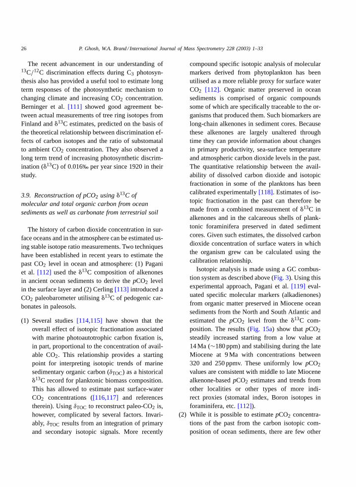
Isotopic analysis is made using a GC combus-tion system as described above (Fig. 3). Using thisexperimental approach, Pagani et al.[119] eval-uated specific molecular markers (alkadienones)from organic matter preserved in Miocene oceansediments from the North and South Atlantic andestimated thepCO2 level from the �13C com-position. The results (Fig. 15a) show thatpCO2
steadily increased starting from a low value at14 Ma (∼180 ppm) and stabilising during the lateMiocene at 9 Ma with concentrations between320 and 250 ppmv. These uniformly lowpCO2
values are consistent with middle to late Miocenealkenone-basedpCO2 estimates and trends fromother localities or other types of more indi-rect proxies (stomatal index, Boron isotopes inforaminifera, etc.[112]).
(2) While it is possible to estimatepCO2 concentra-tions of the past from the carbon isotopic com-position of ocean sediments, there are few other
P. Ghosh, W.A. Brand / International Journal of Mass Spectrometry 228 (2003) 1–33 27
Fig. 15. (a) MaximumpCO2 estimates calculated on the basis of the carbon isotopic composition of the di-unsaturated alkenones. The recordshows an increase inpCO2 concentration during the Miocene period (reproduced from Pagani et al.[141]). (b) Estimated concentrationof atmospheric CO2 (expressed relative to present-day concentration) as a function of time. The points are based on isotopic analysis ofpedogenic carbonates. The dashed curve along with the envelope (error range) is obtained from GEOCARB III (Berner and Kothavala[124]).
28 P. Ghosh, W.A. Brand / International Journal of Mass Spectrometry 228 (2003) 1–33
pCO2 proxies in terrestrial ecosystem, which havebeen used for PhanerozoicpCO2 reconstruction.Pedogenic carbonates have been proposed as anindirect method to estimate the palaeo-CO2 con-centration in the atmosphere[113,120,121]andpalaeosol carbonates are thought to preserve theisotopic composition of local soil CO2; that pri-marily reflecting the type of vegetation (e.g., frac-tion of C3 versus C4 plants (see footnote 2)) inthe ecosystem[100]. Soil CO2 may be consid-ered as mainly a mixture of two components: (i)plant and microbially respired CO2 and (ii) at-mospheric CO2. Mixing of atmospheric CO2 withrespired CO2 is primarily governed by diffusion.Today, except for ecosystems with very low pro-ductivity such as deserts, the atmospheric contri-bution of total soil CO2 is small because of therather low concentration of CO2 in the modernatmosphere compared to that in the soil air. How-ever, at higher atmospheric CO2, as has occurredin the distant past, atmospheric CO2 invasion mayhave made a significant contribution to total soilCO2, this resulting in significant isotopic shiftsin the �13C of soil carbonate precipitated. There-fore, �13C analysis of pedogenic carbonates havebeen taken to provide evidence for large varia-tions in pCO2 in geologic past[119,122,123]. Aknowledge of past carbon dioxide levels and as-sociated paleo-environmental and paleo-ecologicchanges are useful for predicting future conse-quences of the current increase in atmosphericcarbon dioxide.
Estimates of CO2 variations based on equationsgoverning the CO2 outgassing and weathering re-actions are formulated in the GEOCARB II modelof Berner[86] and more recently in GEOCARBIII [124]. Fig. 15b provides the model simula-tion of past CO2 levels. It shows that in the EarlyPhanerozoic (550 Ma) thepCO2 was 20 times thepresent atmospheric level (PAL). Subsequently,pCO2 declined during the Middle and Late Palaeo-zoic (450–280 Ma) to reach a minimum (approx-imately similar to the PAL) at about 300 Ma. Theperiod between 300 and 200 Ma was again char-
acterised by a rapid rise andpCO2 increased to 5times the PAL. It was followed by a gradual de-cline to the PAL with a small peak in the early Ter-tiary. Such large changes inpCO2 in the geologicpast must have had significant impacts upon cli-mate, biota and surface processes on earth[122].Therefore, understanding the nature of variation inatmosphericpCO2 is important for a better under-standing of the Earth’s physical and biotic history.Ghosh et al.[121] determined the atmosphericCO2 concentration using Gondwana soil carbon-ates from India (plotted inFig. 15b). The mean�13C values of the palaeosol carbonates were usedto obtain the individual ranges ofpCO2 values pre-sented in the figure. These values represent firstindependent estimates of atmospheric CO2 lev-els during 260–65 Ma bp from soils formed on the(southern hemisphere) Gondwana supercontinent.This is considered an important period in the evo-lution model as it predicts an increase in the CO2
level after the early Permian low (310–285 Ma)and ascribes it to an enhanced rate of degassing.The figure shows that a reasonable agreement ofthe derived CO2 concentration with Berner’s pre-diction [125] between 275 and 160 Ma has beenobtained. However, the abundance of carbondiox-ide for 65 Ma (Lameta) is 1480 ppm, about twicethe value in Berner’s mass balance model esti-mates (560 Ma, GEOCARB III)[124].
4. Climate models and experimental validation
Climate modelling efforts in general aim at a quan-titative understanding of the processes driving theEarth’s climate system. The complexity of this sys-tem requires to create models that incorporate con-temporary knowledge and that remain open for newinformation from future research. In order to validatean individual model it must be able to reproduceexperimental observations in space and time.9
9 As an introduction to climate modelling we recommend refs.[3,126,127]for further reading.
P. Ghosh, W.A. Brand / International Journal of Mass Spectrometry 228 (2003) 1–33 29
The simplest model is represented by a box. Thebox has source and sink processes for air constituentsincluding chemical reactions and their physicochem-ical properties, water evaporation and condensation,advective processes, radiation, emission from humansources and so on. The size of the box depends onthe problem to be modeled. As an example, the lo-cal climate of an urban environment could be mod-eled by selecting the size of the box slightly largerthan the environment itself and parameterise advec-tion from other information. Alternatively, the envi-ronment could be modeled using a number of smallerboxes communicating their input/output to each otherin order to learn something about the distribution ofa specific pollutant originating from one of the boxeswithin the selected environment over time. The lat-ter approach requires prior knowledge about transportprocesses between the boxes.
The more complex the environment becomes, themore difficult is quantitative modelling. On the otherhand, computing power has increased dramatically inthe past and so has our ability to simulate climate us-ing coupled boxes. The whole atmosphere in currentlyused models is composed of a grid of boxes in all threedimensions with individual properties. In order to cal-culate the varying contents of the boxes over time andspace, the 3D grid is fed with prior information liketrace gas concentration and isotope ratio data fromsampling stations and remote sensing as input vari-ables constraining the calculations of monthly tempo-ral fluxes. The model output delivers information liketemperature, precipitation, etc. The modelling effortsare fine tuned to reproduce the atmospheric trace gasconcentration and seasonal signals from new obser-vations at ground stations. Signals at any monitoringstation can be modeled providing a world wide spa-tial coverage with the option to incorporate new sta-tions or to judge where on earth a new station wouldhave the largest scientific benefit. Model precision in-creases with the number of stations around the globe,with the number of observations on those stations andwith the quality of the data.
Modern climate models can be divided into twobroad categories: (1) general circulation models
(GCM’s) and (2) statistical–dynamical models, whichinclude energy balance models (EBM’s) and two di-mensional zonally averaged dynamic models[124].Both types of models have been used for modellingpalaeoclimatic conditions. GCM’s have been used forsimulating palaeoclimatic processes like precipitation,temperature, etc. which depend mostly on land/seadistribution, atmospheric flow patterns and distribu-tion as well as concentration of aerosols or tracegases in the global atmosphere[128,129]. Statisticaldynamic models have mainly been used for long termclimatic simulation experiments[130–132].
Simulation of sudden events and/or prominent fea-tures in palaeo-climatic records provides a criticaltest for GCM’s [133]. Evaluation of model resultshas opened new opportunities for interdisciplinarypaleoclimate research and simulated (a) the compila-tion of data sets that are global in scope and (b) thedevelopment of increasingly sophisticated methodsfor palaeo-environmental analyses. The data sets andanalyses are routinely used to check the performanceand improve climate models. For example, Kutzbachet al. [134] describe results of climate simulationsfor 21,000, 16,000, 14,000, 11,000 and 6000 yearsbefore present (bp); the output of these simulationexperiments were used for biome (vegetation type)reconstruction. The computer experiments were per-formed using the CCM1 climate model code fromNCAR (National Center for Atmospheric Research inBoulder, CO, USA) which features full annual cyclesimulation, linked with land surface modelling anda mixed layer ocean structure. Introduction of thesefeatures results in a global mean temperature changeat the Last Glacial Maximum (LGM, 18 ka bp) of−6.5◦C compared to today. Overall, the LGM wasfound to be cooler and drier similar to actual observa-tions discussed before. Felzer et al.[135] used NCARCCM1 to isolate the individual effects of orbital forc-ing, ice sheet size and lower CO2 concentration onclimate during and since the LGM. Their study showsthat surface temperatures both globally and region-ally are linear functions of the individual responseto ice sheets, CO2 concentrations and insolation. Atthe LGM, the global mean temperature decrease of
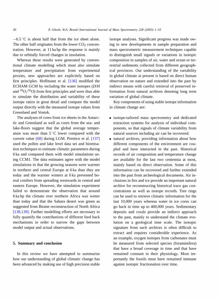
30 P. Ghosh, W.A. Brand / International Journal of Mass Spectrometry 228 (2003) 1–33
−6.5◦C is about half that from the ice sheet alone.The other half originates from the lower CO2 concen-tration. However, at 11 ka bp the response is mainlydue to orbitally forced changes in insolation.
Whereas these results were generated by conven-tional climate modelling which must also simulatetemperature and precipitation from experimentalproxies, new approaches are explicitely based onfirst principles. Hoffmann et al.[136] modified theECHAM GCM by including the water isotopes (D/Hand18O/16O) from first principles and were thus ableto simulate the distribution and variability of theseisotope ratios in great detail and compare the modeloutput directly with the measured isotope values fromGreenland and Vostok.
The analyses of cores from ice sheets in the Antarc-tic and Greenland as well as cores from the sea- andlake-floors suggest that the global average temper-ature was more than 5◦C lower compared with thecurrent value[68] during LGM. Prentice et al.[137]used the pollen and lake level data set and biomisa-tion techniques to estimate climatic parameters during6 ka and compared them with model simulations us-ing CCM1. The data estimates agree with the modelsimulations in that the growing seasons were warmerin northern and central Europe at 6 ka than they aretoday and the warmer winters at 6 ka prevented bo-real conifers from spreading westwards in central andeastern Europe. However, the simulation experimentfailed to demonstrate the observation that around6 ka bp the climate over northern Africa was wetterthan today and that the Sahara desert was green assuggested from Biome reconstruction of North Africa[138,139]. Further modelling efforts are necessary tofully quantify the contributions of different feed backmechanisms in order to narrow the gaps betweenmodel output and actual observations.
5. Summary and conclusion
In this review we have attempted to summarisehow our understanding of global climatic change hasbeen advanced by making use of high precision stable
isotope analyses. Significant progress was made ow-ing to new developments in sample preparation andmass spectrometric measurement techniques capableto distinguish small signals or variations in isotopiccomposition in samples of air, water and ocean or ter-restrial sediments collected from different geograph-ical provinces. Our understanding of the variabilityin global climate at present is based on direct humanobservation on nature and extended into the past byindirect means with careful retrieval of preserved in-formation from natural archives denoting long termvariation of global climate.
Key components of using stable isotope informationin climate change are:
• isotope-tailored mass spectrometry and dedicatedextraction systems for analysis of individual com-ponents, so that signals of climate variability fromnatural sources including air can be recovered.
• natural archives, providing information about howdifferent components of the environment are cou-pled and have interacted in the past. Historicalrecords of air composition and temperature changeare available for the last two centennia at most,mainly based on direct observation. Some of thisinformation can be recovered and further extendedinto the past from archeological documents. Air in-clusions in firn and ice provide an important naturalarchive for reconstructing historical trace gas con-centrations as well as isotope records. Tree ringscan be used to retrieve climatic information for thelast 10,000 years whereas water in ice cores cango back in time up to 400,000 years. Sedimentarydeposits and corals provide an indirect approachto the past, mainly to understand the climate evo-lution on a geological time scale. The isotopicsignature from such archives is often difficult toextract and requires considerable experience. Asan example, oxygen isotopes from carbonates mustbe measured from selected species (foraminifera)that have a broad coverage in time and that haveremained constant in their physiology. Most im-portantly the fossils must have remained immuneagainst isotopic fractionation over time.
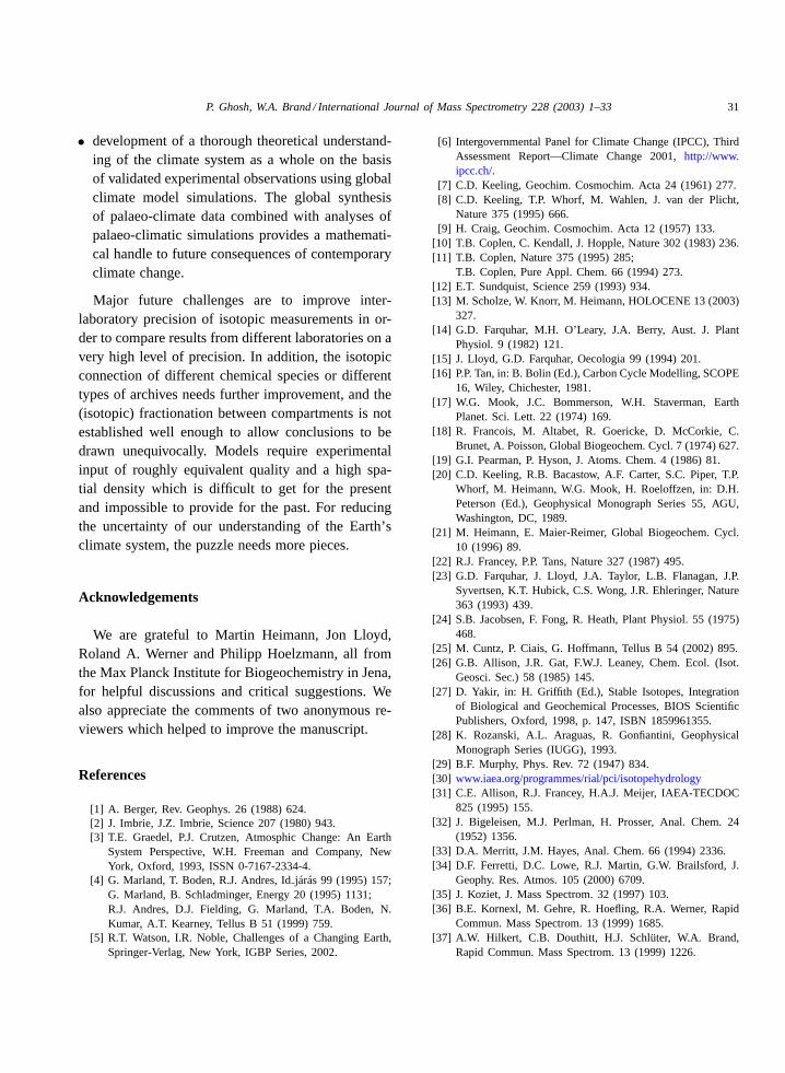
P. Ghosh, W.A. Brand / International Journal of Mass Spectrometry 228 (2003) 1–33 31
• development of a thorough theoretical understand-ing of the climate system as a whole on the basisof validated experimental observations using globalclimate model simulations. The global synthesisof palaeo-climate data combined with analyses ofpalaeo-climatic simulations provides a mathemati-cal handle to future consequences of contemporaryclimate change.
Major future challenges are to improve inter-laboratory precision of isotopic measurements in or-der to compare results from different laboratories on avery high level of precision. In addition, the isotopicconnection of different chemical species or differenttypes of archives needs further improvement, and the(isotopic) fractionation between compartments is notestablished well enough to allow conclusions to bedrawn unequivocally. Models require experimentalinput of roughly equivalent quality and a high spa-tial density which is difficult to get for the presentand impossible to provide for the past. For reducingthe uncertainty of our understanding of the Earth’sclimate system, the puzzle needs more pieces.
Acknowledgements
We are grateful to Martin Heimann, Jon Lloyd,Roland A. Werner and Philipp Hoelzmann, all fromthe Max Planck Institute for Biogeochemistry in Jena,for helpful discussions and critical suggestions. Wealso appreciate the comments of two anonymous re-viewers which helped to improve the manuscript.
References
[1] A. Berger, Rev. Geophys. 26 (1988) 624.[2] J. Imbrie, J.Z. Imbrie, Science 207 (1980) 943.[3] T.E. Graedel, P.J. Crutzen, Atmosphic Change: An Earth
System Perspective, W.H. Freeman and Company, NewYork, Oxford, 1993, ISSN 0-7167-2334-4.
[4] G. Marland, T. Boden, R.J. Andres, Idjárás 99 (1995) 157;G. Marland, B. Schladminger, Energy 20 (1995) 1131;R.J. Andres, D.J. Fielding, G. Marland, T.A. Boden, N.Kumar, A.T. Kearney, Tellus B 51 (1999) 759.
[5] R.T. Watson, I.R. Noble, Challenges of a Changing Earth,Springer-Verlag, New York, IGBP Series, 2002.
[6] Intergovernmental Panel for Climate Change (IPCC), ThirdAssessment Report—Climate Change 2001,http://www.ipcc.ch/.
[7] C.D. Keeling, Geochim. Cosmochim. Acta 24 (1961) 277.[8] C.D. Keeling, T.P. Whorf, M. Wahlen, J. van der Plicht,
Nature 375 (1995) 666.[9] H. Craig, Geochim. Cosmochim. Acta 12 (1957) 133.
[10] T.B. Coplen, C. Kendall, J. Hopple, Nature 302 (1983) 236.[11] T.B. Coplen, Nature 375 (1995) 285;
T.B. Coplen, Pure Appl. Chem. 66 (1994) 273.[12] E.T. Sundquist, Science 259 (1993) 934.[13] M. Scholze, W. Knorr, M. Heimann, HOLOCENE 13 (2003)
327.[14] G.D. Farquhar, M.H. O’Leary, J.A. Berry, Aust. J. Plant
Physiol. 9 (1982) 121.[15] J. Lloyd, G.D. Farquhar, Oecologia 99 (1994) 201.[16] P.P. Tan, in: B. Bolin (Ed.), Carbon Cycle Modelling, SCOPE
16, Wiley, Chichester, 1981.[17] W.G. Mook, J.C. Bommerson, W.H. Staverman, Earth
Planet. Sci. Lett. 22 (1974) 169.[18] R. Francois, M. Altabet, R. Goericke, D. McCorkie, C.
Brunet, A. Poisson, Global Biogeochem. Cycl. 7 (1974) 627.[19] G.I. Pearman, P. Hyson, J. Atoms. Chem. 4 (1986) 81.[20] C.D. Keeling, R.B. Bacastow, A.F. Carter, S.C. Piper, T.P.
Whorf, M. Heimann, W.G. Mook, H. Roeloffzen, in: D.H.Peterson (Ed.), Geophysical Monograph Series 55, AGU,Washington, DC, 1989.
[21] M. Heimann, E. Maier-Reimer, Global Biogeochem. Cycl.10 (1996) 89.
[22] R.J. Francey, P.P. Tans, Nature 327 (1987) 495.[23] G.D. Farquhar, J. Lloyd, J.A. Taylor, L.B. Flanagan, J.P.
Syvertsen, K.T. Hubick, C.S. Wong, J.R. Ehleringer, Nature363 (1993) 439.
[24] S.B. Jacobsen, F. Fong, R. Heath, Plant Physiol. 55 (1975)468.
[25] M. Cuntz, P. Ciais, G. Hoffmann, Tellus B 54 (2002) 895.[26] G.B. Allison, J.R. Gat, F.W.J. Leaney, Chem. Ecol. (Isot.
Geosci. Sec.) 58 (1985) 145.[27] D. Yakir, in: H. Griffith (Ed.), Stable Isotopes, Integration
of Biological and Geochemical Processes, BIOS ScientificPublishers, Oxford, 1998, p. 147, ISBN 1859961355.
[28] K. Rozanski, A.L. Araguas, R. Gonfiantini, GeophysicalMonograph Series (IUGG), 1993.
[29] B.F. Murphy, Phys. Rev. 72 (1947) 834.[30] www.iaea.org/programmes/rial/pci/isotopehydrology[31] C.E. Allison, R.J. Francey, H.A.J. Meijer, IAEA-TECDOC
825 (1995) 155.[32] J. Bigeleisen, M.J. Perlman, H. Prosser, Anal. Chem. 24
(1952) 1356.[33] D.A. Merritt, J.M. Hayes, Anal. Chem. 66 (1994) 2336.[34] D.F. Ferretti, D.C. Lowe, R.J. Martin, G.W. Brailsford, J.
Geophy. Res. Atmos. 105 (2000) 6709.[35] J. Koziet, J. Mass Spectrom. 32 (1997) 103.[36] B.E. Kornexl, M. Gehre, R. Hoefling, R.A. Werner, Rapid
Commun. Mass Spectrom. 13 (1999) 1685.[37] A.W. Hilkert, C.B. Douthitt, H.J. Schlüter, W.A. Brand,
Rapid Commun. Mass Spectrom. 13 (1999) 1226.
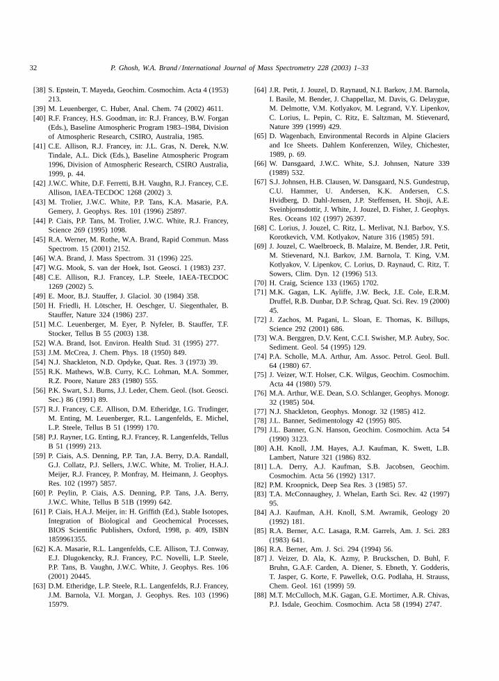
32 P. Ghosh, W.A. Brand / International Journal of Mass Spectrometry 228 (2003) 1–33
[38] S. Epstein, T. Mayeda, Geochim. Cosmochim. Acta 4 (1953)213.
[39] M. Leuenberger, C. Huber, Anal. Chem. 74 (2002) 4611.[40] R.F. Francey, H.S. Goodman, in: R.J. Francey, B.W. Forgan
(Eds.), Baseline Atmospheric Program 1983–1984, Divisionof Atmospheric Research, CSIRO, Australia, 1985.
[41] C.E. Allison, R.J. Francey, in: J.L. Gras, N. Derek, N.W.Tindale, A.L. Dick (Eds.), Baseline Atmospheric Program1996, Division of Atmospheric Research, CSIRO Australia,1999, p. 44.
[42] J.W.C. White, D.F. Ferretti, B.H. Vaughn, R.J. Francey, C.E.Allison, IAEA-TECDOC 1268 (2002) 3.
[43] M. Trolier, J.W.C. White, P.P. Tans, K.A. Masarie, P.A.Gemery, J. Geophys. Res. 101 (1996) 25897.
[44] P. Ciais, P.P. Tans, M. Trolier, J.W.C. White, R.J. Francey,Science 269 (1995) 1098.
[45] R.A. Werner, M. Rothe, W.A. Brand, Rapid Commun. MassSpectrom. 15 (2001) 2152.
[46] W.A. Brand, J. Mass Spectrom. 31 (1996) 225.[47] W.G. Mook, S. van der Hoek, Isot. Geosci. 1 (1983) 237.[48] C.E. Allison, R.J. Francey, L.P. Steele, IAEA-TECDOC
1269 (2002) 5.[49] E. Moor, B.J. Stauffer, J. Glaciol. 30 (1984) 358.[50] H. Friedli, H. Lötscher, H. Oeschger, U. Siegenthaler, B.
Stauffer, Nature 324 (1986) 237.[51] M.C. Leuenberger, M. Eyer, P. Nyfeler, B. Stauffer, T.F.
Stocker, Tellus B 55 (2003) 138.[52] W.A. Brand, Isot. Environ. Health Stud. 31 (1995) 277.[53] J.M. McCrea, J. Chem. Phys. 18 (1950) 849.[54] N.J. Shackleton, N.D. Opdyke, Quat. Res. 3 (1973) 39.[55] R.K. Mathews, W.B. Curry, K.C. Lohman, M.A. Sommer,
R.Z. Poore, Nature 283 (1980) 555.[56] P.K. Swart, S.J. Burns, J.J. Leder, Chem. Geol. (Isot. Geosci.
Sec.) 86 (1991) 89.[57] R.J. Francey, C.E. Allison, D.M. Etheridge, I.G. Trudinger,
M. Enting, M. Leuenberger, R.L. Langenfelds, E. Michel,L.P. Steele, Tellus B 51 (1999) 170.
[58] P.J. Rayner, I.G. Enting, R.J. Francey, R. Langenfelds, TellusB 51 (1999) 213.
[59] P. Ciais, A.S. Denning, P.P. Tan, J.A. Berry, D.A. Randall,G.J. Collatz, P.J. Sellers, J.W.C. White, M. Trolier, H.A.J.Meijer, R.J. Francey, P. Monfray, M. Heimann, J. Geophys.Res. 102 (1997) 5857.
[60] P. Peylin, P. Ciais, A.S. Denning, P.P. Tans, J.A. Berry,J.W.C. White, Tellus B 51B (1999) 642.
[61] P. Ciais, H.A.J. Meijer, in: H. Griffith (Ed.), Stable Isotopes,Integration of Biological and Geochemical Processes,BIOS Scientific Publishers, Oxford, 1998, p. 409, ISBN1859961355.
[62] K.A. Masarie, R.L. Langenfelds, C.E. Allison, T.J. Conway,E.J. Dlugokencky, R.J. Francey, P.C. Novelli, L.P. Steele,P.P. Tans, B. Vaughn, J.W.C. White, J. Geophys. Res. 106(2001) 20445.
[63] D.M. Etheridge, L.P. Steele, R.L. Langenfelds, R.J. Francey,J.M. Barnola, V.I. Morgan, J. Geophys. Res. 103 (1996)15979.
[64] J.R. Petit, J. Jouzel, D. Raynaud, N.I. Barkov, J.M. Barnola,I. Basile, M. Bender, J. Chappellaz, M. Davis, G. Delaygue,M. Delmotte, V.M. Kotlyakov, M. Legrand, V.Y. Lipenkov,C. Lorius, L. Pepin, C. Ritz, E. Saltzman, M. Stievenard,Nature 399 (1999) 429.
[65] D. Wagenbach, Environmental Records in Alpine Glaciersand Ice Sheets. Dahlem Konferenzen, Wiley, Chichester,1989, p. 69.
[66] W. Dansgaard, J.W.C. White, S.J. Johnsen, Nature 339(1989) 532.
[67] S.J. Johnsen, H.B. Clausen, W. Dansgaard, N.S. Gundestrup,C.U. Hammer, U. Andersen, K.K. Andersen, C.S.Hvidberg, D. Dahl-Jensen, J.P. Steffensen, H. Shoji, A.E.Sveinbjornsdottir, J. White, J. Jouzel, D. Fisher, J. Geophys.Res. Oceans 102 (1997) 26397.
[68] C. Lorius, J. Jouzel, C. Ritz, L. Merlivat, N.I. Barbov, Y.S.Korotkevich, V.M. Kotlyakov, Nature 316 (1985) 591.
[69] J. Jouzel, C. Waelbroeck, B. Malaize, M. Bender, J.R. Petit,M. Stievenard, N.I. Barkov, J.M. Barnola, T. King, V.M.Kotlyakov, V. Lipenkov, C. Lorius, D. Raynaud, C. Ritz, T.Sowers, Clim. Dyn. 12 (1996) 513.
[70] H. Craig, Science 133 (1965) 1702.[71] M.K. Gagan, L.K. Ayliffe, J.W. Beck, J.E. Cole, E.R.M.
Druffel, R.B. Dunbar, D.P. Schrag, Quat. Sci. Rev. 19 (2000)45.
[72] J. Zachos, M. Pagani, L. Sloan, E. Thomas, K. Billups,Science 292 (2001) 686.
[73] W.A. Berggren, D.V. Kent, C.C.I. Swisher, M.P. Aubry, Soc.Sediment. Geol. 54 (1995) 129.
[74] P.A. Scholle, M.A. Arthur, Am. Assoc. Petrol. Geol. Bull.64 (1980) 67.
[75] J. Veizer, W.T. Holser, C.K. Wilgus, Geochim. Cosmochim.Acta 44 (1980) 579.
[76] M.A. Arthur, W.E. Dean, S.O. Schlanger, Geophys. Monogr.32 (1985) 504.
[77] N.J. Shackleton, Geophys. Monogr. 32 (1985) 412.[78] J.L. Banner, Sedimentology 42 (1995) 805.[79] J.L. Banner, G.N. Hanson, Geochim. Cosmochim. Acta 54
(1990) 3123.[80] A.H. Knoll, J.M. Hayes, A.J. Kaufman, K. Swett, L.B.
Lambert, Nature 321 (1986) 832.[81] L.A. Derry, A.J. Kaufman, S.B. Jacobsen, Geochim.
Cosmochim. Acta 56 (1992) 1317.[82] P.M. Kroopnick, Deep Sea Res. 3 (1985) 57.[83] T.A. McConnaughey, J. Whelan, Earth Sci. Rev. 42 (1997)
95.[84] A.J. Kaufman, A.H. Knoll, S.M. Awramik, Geology 20
(1992) 181.[85] R.A. Berner, A.C. Lasaga, R.M. Garrels, Am. J. Sci. 283
(1983) 641.[86] R.A. Berner, Am. J. Sci. 294 (1994) 56.[87] J. Veizer, D. Ala, K. Azmy, P. Bruckschen, D. Buhl, F.
Bruhn, G.A.F. Carden, A. Diener, S. Ebneth, Y. Godderis,T. Jasper, G. Korte, F. Pawellek, O.G. Podlaha, H. Strauss,Chem. Geol. 161 (1999) 59.
[88] M.T. McCulloch, M.K. Gagan, G.E. Mortimer, A.R. Chivas,P.J. Isdale, Geochim. Cosmochim. Acta 58 (1994) 2747.
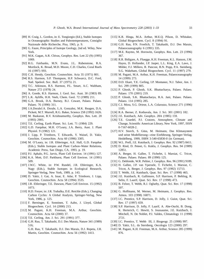
P. Ghosh, W.A. Brand / International Journal of Mass Spectrometry 228 (2003) 1–33 33
[89] H. Craig, L. Gordon, in: E. Tongiorgio (Ed.), Stable Isotopesin Oceanographic Studies and Paleotemperatures, ConsiglioNazionale delle Richerche, Pisa, 1965, p. 9.
[90] G. Faure, Principles of Isotope Geology, 2nd ed. Wiley, NewYork.
[91] M.K. Gagan, A.R. Chivas, Geophys. Res. Lett 22 (9) (1995)1069.
[92] R.G. Fairbanks, M.N. Evans, J.L. Rubenstone, R.A.Mortlock, K. Broad, M.D. Moore, C.D. Charles, Coral Reefs16 (1997) S93.
[93] C.H. Hendy, Geochim. Cosmochim. Acta 35 (1971) 801.[94] R.S. Harmon, S.P. Thompson, H.P. Schwarcz, D.C. Ford,
Natl. Speleol. Soc. Bull. 37 (1975) 21.[95] T.C. Atkinson, R.S. Harmon, P.L. Smart, A.C. Waltham,
Nature 272 (1978) 24.[96] A. Goede, R.S. Harmon, J. Geol. Soc. Aust. 30 (1983) 89.[97] L.K. Ayliffe, H.H. Veeh, Chem. Geol. 72 (1989) 211.[98] G.A. Brook, D.A. Burney, B.J. Cowart, Palaeo. Palaeo.
Palaeo. 76 (1990) 311.[99] J.A.DoraleJ.A. Dorale, L.A. Gonzalez, M.K. Reagen, D.A.
Pickett, M.T. Murrell, R.G. Baker, Science 258 (1992) 1626.[100] M. Baskaran, R.V. Krishnamurthy, Geophys. Res. Lett. 20
(1993) 2905.[101] T.E. Cerling, Earth Planet. Sci. Lett. 71 (1984) 229.[102] G.D. Farquhar, M.H. O’Leary, J.A. Berry, Aust. J. Plant
Physiol. 9 (1982) 121.[103] J. Lipp, P. Trimborn, T. Edwards, Y. Waisel, D. Yakir,
Geochim. Cosmochim. Acta 60 (1996) 3305.[104] M. O’Leary, in: J.R. Ehleringer, A.E. Hall, G.D. Farquhar
(Eds.), Stable Isotopes and Plant Carbon–Water Relations,Academic Press, San Diego, CA, 1993, p. 19.
[105] P.J. Aphalo, P.G. Jarvis, Plant Cell Environ. 14 (1991) 127.[106] K.A. Mott, D.F. Parkhurst, Plant Cell Environ. 14 (1991)
509.[107] J.W.C. White, in: P.W. Rundel, J.R. Ehleringer, K.A.
Nagy (Eds.), Stable Isotopes in Ecological Research,Springer-Verlag, New York, 1989, p. 143.
[108] D. Yakir, J. Gat, A. Issar, E. Adar, P. Trimborn, J. Lipp,Geochim. Cosmochim. Acta 58 (1994) 3535.
[109] J.R. Ehleringer, T.E. Dawson, Plant Cell Environ. 15 (1992)1073.
[110] H.D. Freyer, in: J.R. Trabalka, D.E. Reichle (Eds.), ChangingCarbon Cycles: A Global Analysis, Springer-Verlag, NewYork, 1986, p. 125.
[111] F. Berninger, E. Sonninen, T. Aalto, J. Lloyd, GlobalBiogeochem. Cycl. 14 (2000) 213.
[112] M. Pagani, K.H. Freeman, M.A. Arthur, Geochim.Cosmochim. Acta 64 (2000) 37.
[113] T.E. Cerling, Am. J. Sci. 291 (1991) 377.[114] G.H. Rau, T. Takahashi, D.J. Des Marais, Nature 341 (1989)
516;G.H. Rau, T. Takahashi, D.J. Des Marais, D.J. Repeta, J.H.Martin, Geochim. Cosmochim. Acta 56 (1992) 1413.
[115] K.R. Hinga, M.A. Arthur, M.E.Q. Pilson, D. Whitaker,Global Biogeochem. Cycl. 8 (1994) 91.
[116] G.H. Rau, P.N. Froelich, T. Takahashi, D.J. Des Marais,Palaeoceanography 6 (1991) 335.
[117] M.E. Raymo, M. Horowitz, Geophys. Res. Lett. 23 (1996)367.
[118] R.R. Bidigare, A. Fluegge, K.H. Freeman, K.L. Hanson, J.M.Hayes, D. Hollander, J.P. Jasper, L.L. King, E.A. Laws, J.Milder, F.J. Millero, R. Pancost, B.N. Popp, P.A. Steinberg,S.G. Wakeham, Global Biogeochem. Cycl. 11 (1997) 279.
[119] M. Pagani, M.A. Arthur, K.H. Freeman, Palaeoceanography14 (1999) 273.
[120] D.D. Ekart, T.E. Cerling, I.P. Montanez, N.J. Tabor, Am. J.Sci. 299 (1999) 805.
[121] P. Ghosh, P. Ghosh, S.K. Bhattacharya, Palaeo. Palaeo.Palaeo. 170 (2001) 219.
[122] P. Ghosh, S.K. Bhattacharya, R.A. Jani, Palaeo. Palaeo.Palaeo. 114 (1995) 285.
[123] C.I. Mora, S.G. Driese, L.A. Colarusso, Science 271 (1996)1105.
[124] R.A. Berner, Z. Kothavala, Am. J. Sci. 301 (2001) 182.[125] J.E. Kutzbach, Adv. Geophys. 28A (1985) 159.[126] T.E. Graedel, P.J. Crutzen, Atmosphere, Climate and
Change, Scientific American Library, New York, 1997, ISSN0-7167-6028-2.
[127] H.V. Storch, S. Güss, M. Heimann, Das Klimasystemund seine Modellierung—eine Einführung, Springer-Verlag,Heidelberg, 1999, ISBN 3-540-65830-0 (in German).
[128] W.L. Prell, J.E. Kutzbach, J. Geophys. Res. 92 (1987) 8411.[129] D. Rind, D. Peteet, G. Kukla, J. Geophys. Res. 94 (1989)
12851.[130] A. Berger, H. Gallee, T. Fichefet, I. Marsiat, C. Tricot,
Palaeo. Palaeo. Palaeo. 89 (1990) 125.[131] G. Deblonde, W.R. Peltier, J. Geophys. Res. 96 (1991) 9189.[132] H. Gallee, J.P. van Ypersele, T. Fichefet, I. Marsiat, C.
Tricot, A. Berger, J. Geophys. Res. 97 (1992) 15713.[133] T. Webb, J.E. Kutzbach, Quat. Sci. Rev. 17 (1998) 465.[134] J.E. Kutzbach, R. Gallimore, S.P. Harrison, P. Behling, R.
Selin, F. Laarif, Quat. Sci. Rev. 17 (1998) 473.[135] B. Felzer, T. Webb, R.J. Oglseby, Quat. Sci. Rev. 17 (1998)
507.[136] G. Hoffmann, M. Werner, M. Heimann, J. Geophys. Res.
Atmos. 103 (1998) 16871.[137] I.C. Prentice, S.P. Harrison, D. Jolly, J. Guiot, Quat. Sci.
Rev. 17 (1997) 659.[138] S.P. Harrison, D. Jolly, F. Laarif, A. Abe-Ouchi, B. Dong,
K. Herterich, C. Hewitt, S. Joussaume, J.E. Kutzbach, J.Mitchell, N. De Noblet, P.J. Valdes, Climatology 11 (1998)2721.
[139] I.C. Prentice, T. Webb III, J. Biogeogr. 25 (1998) 997.[140] D. Yakir, S.L. da Sternberg, Oecologia 123 (2000) 297.[141] M. Pagani, K.H. Freeman, M.A. Arthur, Science 285 (1999)
876.


![A Stable-Isotope Mass Spectrometry-Based Metabolic ... · community [15]. Identifying and characterizing the phytoplankton “footprint” from the complex background of dissolved](https://img.pdfslide.net/doc/110x75/5ed95607f59b0f56f45f4c7d/a-stable-isotope-mass-spectrometry-based-metabolic-community-15-identifying.jpg)