1

Stable Partial Agglomeration in a New Economic Geography model

with Agglomeration Costs.

Sylvain Barde and John Peirson

OFCE – DRIC & Department of Economics, University of Kent

Abstract

This study develops a model of location with agglomeration costs based on the

standard New Economic Geography (NEG) framework of Puga (1999), in order to bring

the location predictions of NEG in line with the stylised fact that full agglomeration in a

region is unlikely to occur. The central finding is that the presence of such

agglomeration costs significantly alters the agglomeration properties of the standard

NEG framework. In particular, partial agglomeration becomes a stable long run

outcome in both with and without migration. Furthermore, the level of sensitivity of the

stability predictions to the agglomeration cost market parameters is shown to be

different in on the presence or absence of migration. This outlines the need to evaluate

the imperfectness of migration when modifying the agglomeration costs as a policy

implication

JEL Classification: R11, R12, F12

Keywords: Agglomeration, new economic geography, migration, agglomeration costs

Address for Correspondence: OFCE – DRIC, 250 Rue Albert Einstein, 06560 Valbonne, France. Telephone: 04 93 95 42 38 Email: sylvain.barde@ofce.sciences-po.fr Acknowledgements: The authors are very grateful for the comments and suggestions of Henry Overman, Roger Vickerman and participants to the 2008 ERSA conference.

2

Stable partial agglomeration in a New Economic Geography model

with Agglomeration Costs.

1. Introduction

It is commonly suggested that a stylised fact of economic development is that

complete concentration of industrial activity in a single region is unlikely, e.g.

Ottaviano and Thisse (2004, p.2567) suggest that “full agglomeration and full

dispersion … does not strike us as being plausible”. Thus, it is important to explain

stable partial agglomeration in models of industrial location. However, according to

recent work by Robert-Nicoud (2004) and Ottaviano and Robert-Nicoud (2006, p15),

“an uneven spatial distribution of manufacturing [in New Economic Geography

models], short of full agglomeration … is always unstable”. A range of studies of

studies have nevertheless made alternative assumptions that lead to a conclusion of

stable partial agglomeration, such as Breukner and Zenou (1999), Duranton and Puga

(2004), Epifani and Gancia (2005) or Murata and Thisse (2005)1. The first aim of the

current paper is to consider two possible mechanisms that lead to stable partial

agglomeration: diseconomies of scale external to the firm and agglomeration costs

related to the size of the industry.

The second aim of this paper is to explain how the concentration of workers in

one region gives rise to additional costs that reduce the centripetal force and results in

1 Breukner and Zenou (1999) show that adding a land market to a Harris-Todaro (1970) framework provides extra frictions due to urbanisation, which limits migration. Murata and Thisse (2005) show that a more integrated economy, with lower transport costs, will only be agglomerated if associated labour commuting costs are low. Similarly, Duranton and Puga (2004) introduce commuting costs into a NEG framework, and find that the “the efficient size of a city is the result of a trade-off between urban agglomeration economies and urban crowding”. Finally, Epifani and Gancia (2005) extend this by integrating a full labour market search model into a Krugman (1991) model. Although their goal is to investigate the effect of labour mobility on regional unemployment disparities, they also report stable partial agglomeration.

3

stable partial equilibria. This analysis uses a Dixit-Stiglitz NEG model of

agglomeration. The present analysis and those of Robert-Nicoud (2004) and Ottaviano

and Robert-Nicoud (2006) are compared and explained. It is shown that for the latter

two studies partial agglomeration does not occur because, as firms cluster, wage costs

increase more slowly than revenue.

The NEG model used in the present study develops the framework of Puga

(1999) to include agglomeration costs borne by all workers in the agglomerated region.

The model predicts stable partial agglomeration equilibria for all but low agglomeration

costs. The Puga model is chosen as the basis of the agglomeration costs model as the

original framework explicitly integrates vertical linkages and considers both migration

and non-migration. Robert-Nicoud (2004) considers the Puga model as a key element of

the NEG literature because it provides a full analytical solution of the stability of the

equilibria in terms of parameters and transport costs. In addition, Robert-Nicoud (2004,

p. 3) suggests that only symmetric or complete agglomeration equilibria are stable in

standard NEG models, but that “the current literature would be incomplete if there

existed other stable equilibria”. Brakman et al (1999) show, using a Dixit-Stiglitz model

of agglomeration with diseconomies of scale, that industrial activity is distributed over a

number of cities which can be simply interpreted as a stable partial agglomeration

equilibrium. Thus, we arrive at the general finding that agglomeration costs borne either

by the firm (through diseconomies of scale) or the urbanised region workers can lead to

stable partial agglomeration.

The remained of the paper is organised as follows: section 2 develops the

original Puga (1999) framework to include an agglomeration cost borne by workers in

the urbanised region. The simulations of the migration and non-migrations versions of

the agglomeration cost model are then presented in sections 3 and 4. Section 5 discusses

the implications of these results and section 6 concludes.

4

2. The agglomeration cost model

In order to explain partial agglomeration in NEG, it is necessary to model a

centrifugal force of sufficient magnitude to offset exactly the centripetal force. For such

equilibria to be stable requires additionally that the centrifugal force be dominant at

greater concentrations of activity and centripetal force to be larger at lower

concentrations. A mechanism that could achieve such outcomes is a cost that increases

with agglomeration. This cost may be borne either by the firms or workers. Brakman et

al (1999) in a Dixit-Stiglitz model of location specify the fixed and marginal costs of

production to depend on the number of industrial firms in the region. This model is used

to explain the existence and ranking of several cities, which is equivalent to a stable

partial agglomeration equilibrium. Alternatively, the costs of agglomeration can be

assumed to be borne by the workers, either those in the industrial sector or all workers

in the urbanised region. Ottaviano and Thisse (2004), in particular, strongly suggest the

possibility of workers bearing a cost of agglomeration.

In the present study, the agglomeration of the manufacturing sector in the Puga

model (1999) is assumed to impose a cost on each region in relation to the size of the

manufacturing sector in that region. The burden of this regional agglomeration cost is

then assumed to be equally shared between all the workers in the region. This creates a

simple setting, in which agglomeration of manufacturing in one region is matched by a

relatively higher agglomeration cost and by a lower cost in the region with less

manufacturing activity.

It is assumed that the agglomeration costs are borne by all workers in each

region and are related positively to the size of the manufacturing sector. Several types of

agglomeration costs are relevant. The scarcity of land in areas of high agglomeration

typically results in increased accommodation costs. Agglomeration is likely to put

5

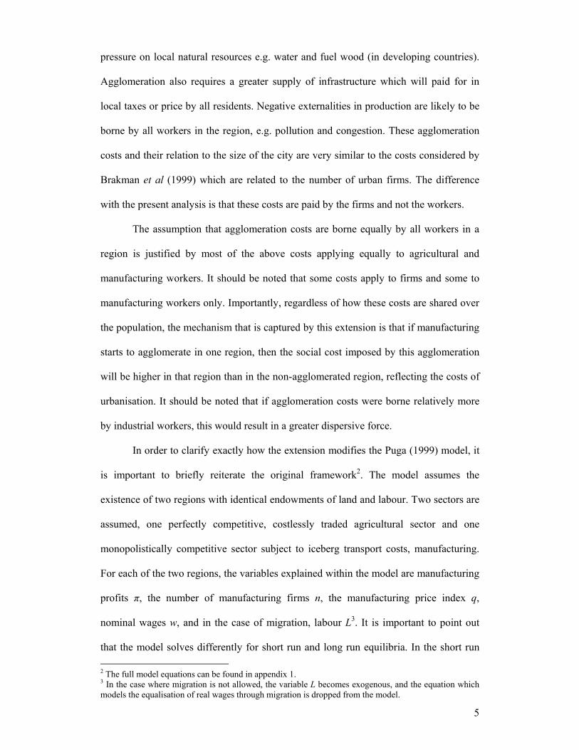
pressure on local natural resources e.g. water and fuel wood (in developing countries).

Agglomeration also requires a greater supply of infrastructure which will paid for in

local taxes or price by all residents. Negative externalities in production are likely to be

borne by all workers in the region, e.g. pollution and congestion. These agglomeration

costs and their relation to the size of the city are very similar to the costs considered by

Brakman et al (1999) which are related to the number of urban firms. The difference

with the present analysis is that these costs are paid by the firms and not the workers.

The assumption that agglomeration costs are borne equally by all workers in a

region is justified by most of the above costs applying equally to agricultural and

manufacturing workers. It should be noted that some costs apply to firms and some to

manufacturing workers only. Importantly, regardless of how these costs are shared over

the population, the mechanism that is captured by this extension is that if manufacturing

starts to agglomerate in one region, then the social cost imposed by this agglomeration

will be higher in that region than in the non-agglomerated region, reflecting the costs of

urbanisation. It should be noted that if agglomeration costs were borne relatively more

by industrial workers, this would result in a greater dispersive force.

In order to clarify exactly how the extension modifies the Puga (1999) model, it

is important to briefly reiterate the original framework2. The model assumes the

existence of two regions with identical endowments of land and labour. Two sectors are

assumed, one perfectly competitive, costlessly traded agricultural sector and one

monopolistically competitive sector subject to iceberg transport costs, manufacturing.

For each of the two regions, the variables explained within the model are manufacturing

profits π, the number of manufacturing firms n, the manufacturing price index q,

nominal wages w, and in the case of migration, labour L3. It is important to point out

that the model solves differently for short run and long run equilibria. In the short run 2 The full model equations can be found in appendix 1. 3 In the case where migration is not allowed, the variable L becomes exogenous, and the equation which models the equalisation of real wages through migration is dropped from the model.

6

the firm mass in is assumed to be fixed, and the system of equations determines iw , iq

and iπ as well as iL in the migration case. In the long run, firm entry or exit in each of

the two regions ensures 0iπ = , and the system can then determine the long run

equilibrium values for iw , iq , in , and iL . In all the simulations carried out in the present

study, the agglomeration cost model parameters are the same as those used in Puga

(1999)4.

Typically in the NEG, the city is where manufacturing activity takes place and

cities are located in regions which always contain agricultural land and activity5. In a

given region the agglomeration costs resulting from the existence of a city therefore

depend on the size of the manufacturing sector in that region. This cost depends first of

all on the number of manufacturing workers located in that region. Secondly, it includes

in ,the number of manufacturing sector firms located in region i. The measure of the size

of the city C in region i is therefore:

( ) ( )( )11i i i i i i iC n q w w nµ µµ σ π− −= − + −1 + (1)

The first part of this equation is the number of manufacturing workers in i, given by the

demand for labour per firm, multiplied by the number of firms. The per capita

agglomeration cost ic is assumed to be a positive function of city size:

( )i ic C ϕχ= (2)

Equations (1) and (2) are therefore added to the existing Puga model. The positive

parameter ϕ is included to allow for the fact that the effect of city size on agglomeration

costs may be non-linear, and χ is a calibration parameter which quantifies how much an

increase in city size increases the per-capita costs of agglomeration.

4 For the migration version, these are 4σ = , 0.2µ = 0.1γ = , and 0.55θ = . For the case where migration is not allowed, µ is increased to 0.4. 5 This assumption implicitly exists in most of the NEG literature, starting with Krugman (1991), as agglomeration of the footloose manufacturing sector is intended to represent urbanisation.

7

In the original model, all workers in a region earn the same wage at equilibrium,

whether they supply their work to the agricultural or manufacturing sector. Because

they are faced with the same prices, their real wage is also the same. This means that at

equilibrium, the marginal worker is indifferent to working in either sector and there is

no intersectoral adjustment. The assumption that per capita cost of agglomeration is the

same for both industrial and agricultural workers conserves the important property of

equalisation of real wages between sectors at equilibrium. As both workers still earn the

same real wage at equilibrium, the marginal worker is still indifferent between and

changing sectors.

As the per capita agglomeration cost ic is imposed on all of the population of

region i, it enters the model via the disposable income of consumers. It is assumed that

the agglomeration cost directly reduces the wages of workers as a lump sum before the

workers start consuming. The consumer utility function is the same as in Puga (1999),

and there is now a difference between wages w and the disposable income of workers

w-c. Solving the utility maximisation problem gives the aggregate consumer

expenditure on manufactures, where γ is the share of expenditure on manufactures:

( )i i iw c Lγ − (3)

As was the case in the original model, if migration between the regions is

allowed, then in the long run the real wages in both regions will equalise. Including the

effect of agglomeration cost on real wages and the assumption that all workers bear this

cost, the long run equality of the real wages between regions can now be expressed as:

( ) ( )i i i j j jq w c q w cγ γ− −− = − (4)

The simple way in which the agglomeration cost c feeds back into the model

stems from the assumption that both manufacturing and agricultural workers bear the

cost. Because of this, one can write the aggregate consumption of labour as shown in

equation (3), and maintain the analytical simplicity of Puga (1999). This also means that

8

agglomeration cost model still nests the original Puga (1999) model. If the cost share

parameter χ is set to zero, the extra equation (2) reduces to 0c = , the extra variable c

disappears from equations (3) and (4), and the model reverts to the original framework.

This implies, therefore, that the extended model still solves as explained above. Short

run equilibria are computed by setting the firm mass exogenously and solving for

profits. Conversely, setting profits exogenously to zero and solving for the firm mass

allows the calculation of the long run equilibria.

3. Stability of the agglomeration cost model with migration

In the agglomeration cost model with migration, the cost parameters are set

around 0.05 for the cost share χ and at 0.5 for the non-linearity parameter φ. In these

simulations, therefore, the agglomeration costs have a relatively small effect, but it will

nevertheless be shown to be important.6 These central values are chosen because they

are half the size of the cut-off values after which the dispersion is so strong that no

agglomeration occurs.7 In order to provide an element of sensitivity analysis,

simulations were carried out with χ and φ parameters around the values used. Figure 1

shows the long run equilibrium path of the share of manufacturing for the system as a

function of transport agglomeration costs. Two important observations can be made

from the analysis of this figure.

First of all, at the lowest levels of transport cost agglomeration ceases to be a

stable outcome, and manufacturing disperses itself over regions again. This is not the

case in the original model, where there is only one bifurcation away from the symmetric

6 For the central values of χ and φ, per capita agglomeration costs c at the symmetric equilibrium represent just over 4% of the equilibrium wage w, which is the same for all transport costs. 7 Simulations reveal that keeping everything else constant, a value of χ above 0.1 leads to the complete absence of agglomeration. Furthermore, simulations reveal that the maximum value of the non-linear parameter φ for which agglomeration occurs is 0.8.

9

equilibrium, aroundτ =1.6 , and full agglomeration is the only stable outcome for

transport costs below this value. The economic rationale for the bifurcation at low

transport costs follows from equation (3). Agglomeration costs imply a lower

disposable income, which reduces consumer demand for all goods and therefore also

reduces the profitability of locating in a city. We consider a full agglomeration

equilibrium around transport costs of 1.2. With migration, full agglomeration implies a

large city and high per capita agglomeration costs, as all the firms and most of the

labour are located there. As transport cost decrease and manufacturing output increases,

so do nominal wages, attracting even more labour and pushing the agglomeration costs

up again.

As transport costs decrease further, a critical level is passed where it becomes

profitable for a firm to switch regions. The cost of switching regions is importing the

intermediate inputs from the city and exporting the output back, where most of the

demand is still located. This cost decreases with transport costs. The benefit to the

industrial sector as a whole of one firm moving is the increase in consumer expenditure

following the reduction in city size and agglomeration costs. As transport costs

decrease, this benefit increases. The agglomerated city size increases as transport costs

decrease and the net positive effect on expenditure of a firm relocating will be bigger

the lower the transport cost. In this respect, the migration case is similar to the non

migration case, in that the agglomerated equilibrium will disperse when transport costs

fall below a critical level.

The second central observation is that the partially agglomerated portion of the

equilibrium path is now stable in the long run, which was not the case in standard NEG

or in Puga (1999). This can be seen from Figure 2, which provides phase diagrams for

the system. The dark surfaces plot the short manufacturing run profits given transport

costs and the share of industry in the region. Intersections of these surfaces with the

10

φ =

0.6

φ =

0.5

φ =

0.4

Figu

re 1

: Equ

ilibr

ium

pat

h of

the

aggl

omer

atio

n m

odel

, mig

ratio

n ve

rsio

n

χ = 0

.04

χ = 0

.05

χ = 0

.06

11

φ =

0.6

φ =

0.5

φ =

0.4

Figu

re 2

: Sta

bilit

y of

the

equi

libri

um p

ath,

mig

ratio

n ve

rsio

n

χ = 0

.04

χ = 0

.05

χ = 0

.06

12

0iπ = planes provides the locations of the long run equilibria seen in Figure 1.

Assuming an adjustment process whereby firms enter or exit a region in response to

positive or negative profits, one can see that keeping transport costs constant, the

partially agglomerated equilibria are indeed stable. Full agglomeration in one of the two

regions remains the dominant form of agglomeration for most of the values of the χ and

φ parameters; however the paths leading to it are now also stable in the long run. Stable

partial agglomeration is therefore the important result from the inclusion of

agglomeration costs. The relevance of the sensitivity analysis is that it shows that this

stability of the partially agglomerated equilibrium is a property of the agglomeration

cost model, and not the accidental by-product of the parameters chosen.

The reason for this stability is again explained through equation (3). In a

standard NEG model and at the symmetric equilibrium, all variables are equal in both

regions. A sufficient fall in transport costs takes the equilibrium to a break point. At the

break point, if one firm moves from region 2 to region 1, the demand for labour in

region 1 increases slightly, and wages increase. This triggers a small migration of

workers from region 2 to region 1, attracted by the slightly higher wages. Region 1 now

has a greater wage income than region 2, which results in a greater demand for all

goods. This triggers further migration of firms from region 2 to region 1, wanting to

locate closer to this greater demand. This further increases wages and leads to more

migration. As explained by Puga (1999) and Robert-Nicoud (2004), if the wage costs

for firms increase by less than the revenue effect then this process is one of cumulative

causation. This bang-bang effect continues until all the firms are located in region 1.

If agglomeration costs are introduced that reduce disposable income, this bang-

bang property is inhibited. Following a reduction in transport costs, a first firm moves

from region 2 to region 1, wages increase and workers move to follow the firm.

However, this now also increases the agglomeration cost, reducing the amount of wage

13

income spent on goods, as shown by equations (1) to (3). Eventually, the increase in the

wage bill is equal to the increase in the agglomeration cost. Thus, demand for industrial

goods is unchanged and no more firms will want to move. The new outcome is one of

partial equilibrium which is also stable. As suggested by Robert-Nicoud (2004), the

cumulative causation process in standard NEG can be halted by the presence of

sufficient agglomeration costs.

A comparison of the symmetric equilibrium stability condition for the

agglomeration model with the stability condition for the original Puga model is shown

in Figure 3. As in Puga (1999), the stability function is defined as the drop in home

profits following an increase in foreign output minus the drop in home profits 1 2nπ∂ ∂ ,

following an increase in home output 1 1nπ∂ ∂ . In terms of notation, for all transport

costs τ, S is the value of the original stability function and S’ the stability function with

agglomeration costs:

1 1

2 1

Sn nπ π′ ′∂ ∂′ = −∂ ∂

and 1 1

2 1

Sn nπ π∂ ∂

= −∂ ∂

(5)

The nπ∂ ∂ elements of the stability matrix are obtained using the implicit function

method, presented in appendix 2. This is because the inclusion of the per capita

agglomeration cost variable c makes the determination of analytical stability functions

much more complicated by introducing a non-linear feedback of firm mass on itself.

Positive values of the stability function indicate a stable symmetric equilibrium,

and negative values an unstable one. The breakpoints of the system are therefore given

by the roots of the stability function. The comparison of the stability functions reveals

that the presence of an agglomeration cost reduces the range of transport costs over

which agglomeration occurs. Including agglomeration costs borne by workers therefore

seems to reduce the range over which any form of agglomeration is possible, partial or

total. This can be linked to the reduction in consumer disposable income caused by

14

φ =

0.6

φ =

0.5

φ =

0.4

Figu

re 3

: C

ompa

riso

n of

ori

gina

l and

agg

lom

erat

ion

cost

stab

ility

con

ditio

ns, m

igra

tion

vers

ion

χ = 0

.04

χ = 0

.05

χ = 0

.06

15

the introduction of the agglomeration costs and the resulting reduction in consumer

demand. In particular, as shown above, this is what explains the observed instability of

agglomeration for low transport costs. Furthermore, Figure 3 shows that the slope of the

stability function does not seem affected much by the introduction of agglomeration

costs:

S Sτ τ′∂ ∂

∂ ∂ (6)

This indicates that both the diagonal and off-diagonal elements of the stability

matrix are affected symmetrically by variations in transport costs, and variations in their

relative size with respect to transport costs are similar to the original model. Although

the exact position of the curve depends on the value of the parameters, it lies strictly

above the original one without the slope being affected by the extension.

Compared to the migration version of the Puga (1999) model, the extra

dissaglomeration force introduced by the agglomeration cost makes agglomeration less

likely. When agglomeration does, occur, however, it can be both partial and stable in the

long run. This is an important result, as it confirms that including such a cost of

agglomeration can produce a rich range of partial agglomeration outcomes in a NEG

framework, which improves its consistency with the stylised fact mentioned in

introduction.

4. Stability of the agglomeration cost model in the absence of migration

The non-migration version of the agglomeration cost model consists of a

reduced system, because real wages differentials are not equalised across regions and

the corresponding equation is dropped from the model. Again, the main model

parameters for this version are the same as the ones used in the non-migration version of

16

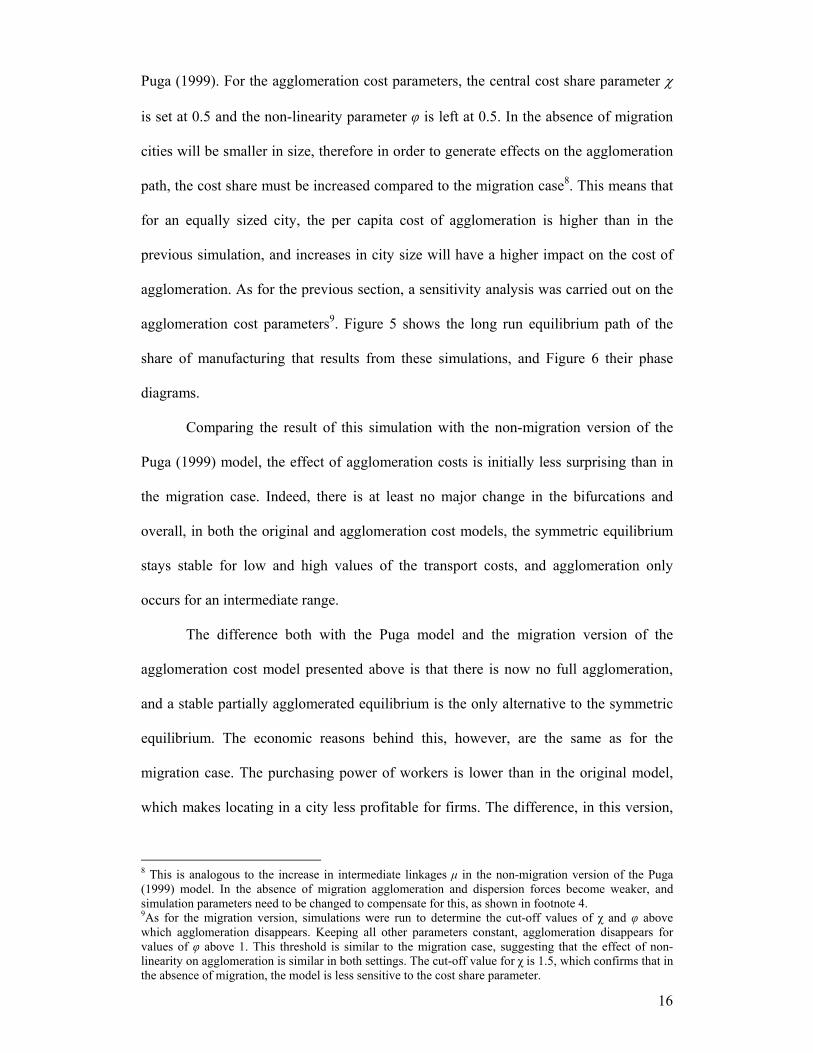
Puga (1999). For the agglomeration cost parameters, the central cost share parameter χ

is set at 0.5 and the non-linearity parameter φ is left at 0.5. In the absence of migration

cities will be smaller in size, therefore in order to generate effects on the agglomeration

path, the cost share must be increased compared to the migration case8. This means that

for an equally sized city, the per capita cost of agglomeration is higher than in the

previous simulation, and increases in city size will have a higher impact on the cost of

agglomeration. As for the previous section, a sensitivity analysis was carried out on the

agglomeration cost parameters9. Figure 5 shows the long run equilibrium path of the

share of manufacturing that results from these simulations, and Figure 6 their phase

diagrams.

Comparing the result of this simulation with the non-migration version of the

Puga (1999) model, the effect of agglomeration costs is initially less surprising than in

the migration case. Indeed, there is at least no major change in the bifurcations and

overall, in both the original and agglomeration cost models, the symmetric equilibrium

stays stable for low and high values of the transport costs, and agglomeration only

occurs for an intermediate range.

The difference both with the Puga model and the migration version of the

agglomeration cost model presented above is that there is now no full agglomeration,

and a stable partially agglomerated equilibrium is the only alternative to the symmetric

equilibrium. The economic reasons behind this, however, are the same as for the

migration case. The purchasing power of workers is lower than in the original model,

which makes locating in a city less profitable for firms. The difference, in this version,

8 This is analogous to the increase in intermediate linkages µ in the non-migration version of the Puga (1999) model. In the absence of migration agglomeration and dispersion forces become weaker, and simulation parameters need to be changed to compensate for this, as shown in footnote 4. 9As for the migration version, simulations were run to determine the cut-off values of χ and φ above which agglomeration disappears. Keeping all other parameters constant, agglomeration disappears for values of φ above 1. This threshold is similar to the migration case, suggesting that the effect of non-linearity on agglomeration is similar in both settings. The cut-off value for χ is 1.5, which confirms that in the absence of migration, the model is less sensitive to the cost share parameter.

17

φ =

0.6

φ =

0.5

φ =

0.4

Figu

re 4

: Equ

ilibr

ium

pat

h of

the

aggl

omer

atio

n m

odel

, non

-mig

ratio

n ve

rsio

n

χ = 0

.4

χ = 0

.5

χ = 0

.6

18

φ =

0.6

φ =

0.5

φ =

0.4

Figu

re 5

: Sta

bilit

y of

the

equi

libri

um p

ath,

non

-mig

ratio

n ve

rsio

n

χ = 0

.4

χ = 0

.5

χ = 0

.6

19

is that because there is no migration, workers are not able to follow firms as they

change regions, making full agglomeration of manufacturing activity much more

difficult. In a situation where a large proportion of manufacturing is located in region 1,

the wages manufacturing firms have to pay will be high, because without migration

labour is scarce. At the same time, the city is relatively large in size because most of the

firms are located there, so the per capita agglomeration costs are high, and a significant

part of the wages paid are not converted into consumer demand. Furthermore, due to the

absence of migration, a large portion of the demand is still located in region 2, and the

goods shipped there are subject to transport costs.

At some point during the agglomeration process, which depends on the

agglomeration cost parameters, it will become profitable for a firm to locate in region 2,

where labour inputs are more plentiful and cheaper, and cater for the demand located

there. At this point, the city located in region 2 has only a small share of manufacturing

firms. Agglomeration costs are therefore lower than in region 1, and more of the region

2 wage bill gets converted into demand. Full agglomeration in one region is therefore

extremely difficult in this case, as the alternative of locating in a region that has cheaper

labour inputs and a relatively high demand will become profitable before full

agglomeration occurs.

The possibility of a stable partially agglomerated path without migration in the

Puga model is not new, as it was shown in Figures 6 and 7 of Puga (1999) that it is

possible to obtain a path similar to the ones in Figure 4. The relevance of the extension

in this case is that the partial agglomeration is achieved with the same structural

parameters as in the Puga (1999) model. The partial agglomeration result of Puga

(1999) relies on an extreme value of the θ parameter, which is set at 0.94. θ being the

elasticity of agricultural output with respect to labour, this implies a highly labour-

intensive agricultural sector, with an elasticity of agricultural output with respect to land

20

of only 0.06. This means that although partial agglomeration can be obtained in the non-

migration version of Puga (1999), it is not a general property of the model, and requires

a very inelastic labour supply to the manufacturing sector. This is not the case here,

where the structural parameters are unchanged compared to the original version of the

Puga model and where the partially agglomerated equilibrium is a widespread result

that stems from agglomeration costs.

Another important finding of the non-migration version of this model is the

effect on the range of transport costs over which the symmetric equilibrium is stable.

Figure 6 shows a comparison of the original and extended stability functions calculated

using the implicit function method. When compared to the migration case in Figure 3, it

is clear that in the absence of migration, the effect of agglomeration costs on the break

points is more complex. The presence of agglomeration costs makes the stability

function steeper rather than translating it upwards, as was the case with migration.

Using the notation used above, if S is the original stability function and S’ is the

agglomeration cost one, one can see from Figure 6 that for most of the range of

transport costs:

S Sτ τ′∂ ∂≥

∂ ∂ (7)

Keeping in mind the definitions of S and S’ in (5), this implies:

2 2 2 2

1 1 1 1

2 1 2 1n n n nπ π π πτ τ τ τ′ ′∂ ∂ ∂ ∂− ≥ −

∂ ∂ ∂ ∂ ∂ ∂ ∂ ∂ (8)

What this shows is that contrary to the migration version, the agglomeration

costs increase the sensitivity to transport costs of the off-diagonal element 1 2nπ∂ ∂

relative to the diagonal element 1 1nπ∂ ∂ . This means that the diagonal and off-diagonal

elements of the stability matrix are now affected asymmetrically by variations in

transport costs, with one being affected more by changes in transport costs than the

21

φ =

0.6

φ =

0.5

φ =

0.4

Figu

re 6

: C

ompa

riso

n of

ori

gina

l and

agg

lom

erat

ion

cost

stab

ility

con

ditio

ns, m

igra

tion

vers

ion

χ = 0

.4

χ = 0

.5

χ = 0

.6

22

other. This is an additional intricacy that is not present in the migration version of the

model, as the slopes of the original and extended stability function are comparable.

For the higher range of transport costs, the effect of the extension on the stability

function is the same as in the migration case. Because consumer demand is constrained

to be spread over regions and transport costs between regions are high, agglomeration

costs decrease disposable income and reduce the profitability of locating in the

agglomerated region. The counter-intuitive aspect is that although the agglomeration

costs reduce consumer spending, agglomeration is now sustainable below the original

Puga (1999) critical point. What explains this sustained agglomeration is that in the

absence of migration and for low values of the transport cost, partial agglomeration can

increase manufacturing profits, and that the presence of the agglomeration cost makes

this partially agglomerated equilibrium stable in the long run.

At the symmetric equilibrium, just to the left of the original lower breakpoint,

the spreading of manufacturing firms across regions means that wages are low. What

underpins the profitability of partial agglomeration is that consumer demand is lower

than in the presence of agglomeration, where the higher labour demand and absence of

migrant labour create higher wages. Therefore, it is profitable for some firms to

agglomerate in one region, and increase consumer demand through higher wages. The

presence of the agglomerated firms also reduces the cost of procuring intermediate

inputs. Furthermore, because of the relatively low level of transport costs, it is possible

to ship the output produced in this small city to the other region, where a lot of the final

demand is still located. Because the agglomeration costs inhibit the bang-bang

transitions of the model, this partial agglomeration equilibrium becomes stable. This

will be the case until the transport cost drops below a certain point, at which point the

dispersion force of being able to costlessly ship intermediate inputs from, and outputs

to, any region will become too strong to make any agglomeration profitable.

23

5. Comparison with the literature and discussion

Section 2 shows that the agglomeration cost model nests the Puga (1999)

framework. What this means is that it is possible to use exactly the same structural

parameters as in Puga (1999) and modify the agglomeration cost independently to

evaluate the effect of the extension. The previous sections show the main result to be

that partial agglomeration becomes stable in the long run. This is an important point for

NEG, in view of recent analytical results in Robert-Nicoud (2004) and Ottaviano and

Robert-Nicoud (2006), which conclude that partial agglomeration is always unstable in

standard Dixit-Stiglitz NEG models. Their result is challenged by the finding that the

general inclusion of agglomeration costs can create stable partial agglomeration whether

they are borne by firms as in Brakman et al (1999), or by workers as is the case here.

This is a point that needs to be explored further, along the lines of the studies mentioned

above, in order to determine how the general agglomeration properties of NEG models

with agglomeration costs are different to those described by Ottaviano and Robert-

Nicoud.

In addition, the simulations show that small changes in agglomeration costs can

have large effects on the location of the agglomeration path. In particular, the sensitivity

of the agglomeration equilibria to the cost parameters is different in the two versions of

the model. This has some important policy implications, as a policy aimed at reducing

the agglomeration costs borne by workers in the agglomerated regions will have a

different effect on agglomeration depending on how free migration is. As mentioned in

Combes et al (2005), the impact of incomplete migration is an aspect of the field that

has received little attention.

24

Another consequence of the complex influence that agglomeration costs have on

the stability function is that studies that test the analytical Puga (1999) breakpoints will

be affected if agglomeration costs are substantial. A first example is the sectoral test of

the Puga breakpoints carried out in Head and Mayer (2004). Using data from two pairs

of countries, USA-Canada and France-Germany, this study calculates the range of

transport costs over which 21 different industrial sectors should be agglomerated. When

comparing the range of transport costs with the actual situation in those sectors, the

finding is that nearly all the industrial sectors should be disaggregated. Head and Mayer

point out that cautious interpretation is needed as the ranges are quite sensitive to the

parameters chosen. Another case is the Brakman et al (2006) test of NEG models,

which uses EU data to test an equilibrium wage equation derived from the Puga model.

This provides estimates for the elasticity σ and the transport costτ . The Puga (1999)

analytical stability function is then used with these estimates to determine the level of

agglomeration in the EU. As is the case in Head and Mayer (2004), Brakman et al

recognise that the assumptions behind the Puga model are unrealistic, and a lot of

further assumptions have to be made in order to get reasonable estimates of the

parameters. The central result of the study, which supports the Head and Mayer (2004)

findings, is that agglomeration forces seem to be too weak to explain the spatial

structure of the EU.

Given the complex interaction of agglomeration costs, migration and partial

agglomeration revealed in the simulations, there is little doubt that taking into account

agglomeration costs would modify the results of Head and Mayer (2004) and Brakman

et al (2006). For example, the relative weakness of agglomeration they find would be

affected, as this study shows that in the absence of migration an agglomeration cost can

push the breakpoints further apart. This is not to say that the problems pointed out in

these two studies would necessarily be solved by this agglomeration model, particularly

25

as far as the number of regions or sectors is concerned, as the present model remains a

simplified NEG framework. However, what is clear is that agglomeration costs of the

kind presented here affect both the range and scope of agglomeration this needs to be

taken into account when testing for agglomeration and dispersion forces.

6. Conclusion

The central finding of this paper is that it is possible to obtain stable partial

agglomeration within a vertically linked Dixit-Stiglitz model by accounting for the extra

social costs of agglomeration. This is true for both the migration and non-migration

versions of the extended framework. Furthermore, simulations using a wider range of

agglomeration cost parameters have shown that whilst the presence of partial

agglomeration is widespread, it is also sensitive to the parameters chosen. This is

especially true for the migration case, where very small changes in the parameters have

large effects in terms of agglomeration.

Importantly, as explained by Robert-Nicoud (2004) and emphasised throughout

the present study, what drives the partial agglomeration result in both cases is the

reduction in the disposable income due to the presence of agglomeration costs. In

standard NEG frameworks all of the wages are spent on goods, which means that as

firms cluster, increases in wages costs are smaller than increases in revenue for the firm.

This cumulative causation mechanism continues until agglomeration in complete. The

model developed in the present study introduces a cost that reduces the disposable

income of workers and reduces demand as a result, making it slightly less profitable for

firms to agglomerate. In the simple framework assumed here, this happens as a result of

an agglomeration cost that is paid for by the entire population. The examples mentioned

26

are pollution or the cost of providing urban infrastructure. However, even with more

complex agglomeration costs and a more realistic spread of these costs it would be

possible to obtain the results shown in this study, as suggested by the result of Brakman

et al (1999), with agglomeration costs borne by firms. What this means is that stable

partial agglomeration can result directly from a reduction in demand due to costs linked

with to the existence and size of a city. Any mechanism which reduces the disposable

income of workers based on the size of the urban area would provide a similar effect.

This has also been shown to have important theoretical consequences on existing new

economic geography theory.

Last of all, in the migration case, the presence of agglomeration costs creates a

dispersion force which reduces range of transport costs over which agglomeration

occurs. The non-migration case, however, is more complex, and comparison of stability

functions shows that depending on the land market parameters the range can be

narrower, or wider than in the initial Puga (1999) specification. This finding calls for a

better understanding of the links between agglomeration and incomplete migration, i.e.

situations where real wage differentials persist over time.

27

References

Brakman S, Garretsen H, Van Marrewijk C, Van den Berg M, “The Return of Zipf :

Towards a Better Understanding of the Rank-Size Distribution”, Journal of

Regional Science, Vol. 39, N° 1, p183-213, 1999.

Brakman S, Garretsen H, Schramm M, “Putting New Economic Geography to the Test:

Free-ness of Trade and Agglomeration in the EU Regions” Regional Science

and Urban Economics, Vol. 36, p613-635, 2006.

Bruekner J.K, Martin R.W, “Spatial Mismatch: An equilibrium analysis”, Regional

Science and Urban Economics, vol. 27 p 693-714, 1997.

Bruekner J.K, Thisse J-F, Zenou Y, “Why is Central Paris Rich and Downtown Detroit

Poor? An Amenity-based Theory”, European Economic Review, Vol.43, p91-

107, 1999.

Bruekner J.K, Thisse J-F, Zenou Y, “Local labour Markets, Job Matching, and urban

Location”, International Economic Review, vol. 43, N° 1, 2002.

Bruekner J.K, Zenou Y, “Harris-Todaro Model with a land market”, Regional Science

and Urban Economics vol. 29 p 317-339, 1999.

Chiang A.C, Fundamental Methods of Mathematical Economics, McGraw-Hill, 3rd ed,

1984

Combes P-P, Duranton G, Overman H.G, “Agglomeration and the Adjustment of the

Spatial Economy”, Papers in Regional Science, Vol. 84, N° 3, p31-349, 2005.

Dixit A.K, Stiglitz J.E, “Monopolistic Competition and Optimum Product Diversity”,

American Economic Review, Vol. 67, N° 3, 977.

Duranton G, Puga D, “Micro-foundations of Urban Agglomeration Economies” The

Handbook of Regional and Urban Economics, J.V.Henderson and J-F Thisse

eds, Vol. IV, 2004.

28

Fujita M, Krugman P, Venables A, The spatial economy; Cities, Regions and

International Trade, MIT press, 1999.

Fujita M, Thisse J-F, “Economics of Agglomeration”, Journal of the Japanese and

International Economies, Vol. 10, p339-378, 1996.

Harris J.R, Todaro M.P, “Migration, unemployment and development: a two-sector

analysis” American Economic Review, Vol. 60, p126-142, 1970.

Head K, Mayer T, “The Empirics of Agglomeration and Trade”, in The Handbook of

Regional and Urban Economics, Vol. IV, p2609-2665, 2004

Krugman P, “Increasing returns and Economic Geography”, Journal of Political

Economics, Vol. 99, Nº 3, 1991.

Murata Y, Thisse J-F, “A Simple Model of Economic Geography à la Helpman-

Tabuchi”, Journal of Urban Economics, Vol. 58, p137-155, 2005.

Ottaviano G, Puga D, “Agglomeration in the global economy: A survey of the ‘new

economic geography’ ”, CEP Disscussion Paper, N° 356, 1997.

Ottaviano G, Robert-Nicoud F “The ‘Genome’ of NEG Models with Vertical Linkages:

A Positive and Normative Synthesis” Journal of Economic Geography, Vol. 6,

Nº 2, p113-139, April 2006.

Ottaviano G, Thisse J-F, “Agglomeration and Economic Geography”, The Handbook of

Regional and Urban Economics, Vol. IV, 2004

Puga D, “The Rise and Fall of Regional Inequalities”, European Economic Review, Vol.

43, 1999.

Robert-Nicoud F, “The Structure of Simple ‘New Economic Geography’ Models (or On

Identical Twins)”, Journal of Economic Geography, Vol. 4, p1-34, 2004.

Samuelson P.A, “The Transfer Problem and Transport Costs: Analysis of Effects of

Trade Impediments”, The Economic Journal, Vol.64, N° 254 p264-289, June

1954.

29

Smith T.E, Zenou Y, “A Discrete-Time Stochastic Model of Job Matching”, Review of

Economics Dynamics, Vol.6, p54-79, 2003.

Smith T.E, Zenou Y, “Spatial Mismatch, Search Effort and Urban Spatial Structure”,

Journal of Urban Economics, Vol. 54, Nº 1, p129-156, July 2003.

Venables A.J, “Equilibrium Locations of Vertically Linked Industries”, International

Economic Review, Vol. 37 Nº 2, p 341-359, May 1996.

Wasmer E, Zenou Y, “Space, Search and Efficiency” IZA Disscussion Paper, N° 181,

2000.

Wasmer E, Zenou Y, “Does City Structure Affect Job Search and Welfare?”, Journal of

Urban Economics, Vol. 51, p515-541, 2002.

Wasmer E, Zenou Y, “Equilibrium Search Unemployment with Explicit Spatial

Frictions”, CEPR Discussion Paper, N° 4743, November 2004.

Zenou Y, “Urban Unemployment and City Formation. Theory and policy Implications”,

Institute for International Economic Studies, Seminar paper N° 662, 1999.

Zenou Y Smith T, “Efficiency wages, involuntary unemployment and urban spatial

structure”, Regional Science and Urban Economics”, vol. 25, p 547-573, 1995.

30

Appendix 1: Puga (1999) and agglomeration cost model equations

The full Puga model, as specified in appendix of Puga (1999) consists of the following

set of equations (A.1)-(A.4), which determine iπ , iw , iq , in , and iL according to the

process mentioned in section 2. For a full explanation of the derivations of these

equations, the reader is referred to Puga (1999).

( ) ( )( )

( ) ( )( ) ( )( ) ( )( ) ( )( )1 1 1

1 1 1

ˆ ˆ

ˆˆ ˆ ˆ ˆ ˆ ˆ1

q w

Tq wL Kr w n nq w q w

µ σ µ σ

σ µ σ µµ σµ

σπ

γ γ µ σ π µ

− − −

− − −

= ×

+ + − − + − (A.1)

( ) ( )( )1 1 11 ˆ ˆ 0µ σ µ σσ − − −− − =q Tq w n (A.2)

( ) ( )( ) ( )1 ˆˆ ˆ ˆ1 0wL n q w w Kr wµ µµ σ π− −− − + −1 + = (A.3)

1 11Tq w q wM

γ γ− −= (A.4)

Given the existing Puga model and the agglomeration cost equations defined in section

2, the agglomeration cost model is described by equations (A.5)-(A.9), and not only

determines iπ , iw , iq , in , and iL , but also the per capita agglomeration cost ic .

( ) ( )( )

( ) ( ) ( )( ) ( )( ) ( )( ) ( )( )1 1 1

1 1 1

ˆ ˆ

ˆˆ ˆ ˆ ˆ ˆ ˆ ˆ1

q w

Tq w c L Kr w n nq w q w

µ σ µ σ

σ µ σ µµ σµ

σπ

γ γ µ σ π µ

− − −

− − −

= ×

− + + − − + − (A.5)

( ) ( )( )1 1 11 ˆ ˆ 0µ σ µ σσ − − −− − =q Tq w n (A.6)

( ) ( )( ) ( )1 ˆˆ ˆ ˆ1 0wL n q w w Kr wµ µµ σ π− −− − + −1 + = (A.7)

( ) ( )( )( )1ˆ ˆ ˆ1c n q w w nϕµ µχ µ σ π− −= − + −1 + (A.8)

( ) ( )1 11Tq w c q w cM

γ γ− −− = − (A.9)

31

Appendix 2: An implicit function method for determining stability

This appendix explains the numerical methodology developed to asses the effect

of the extension on the stability of the symmetric equilibrium. This methodology is

based on the fact that most of the numerical solvers used for simulating problems such

as the system (A.1)-(A.4) require that it be re-arranged in the form shown in (A.7), by

subtracting the right hand side from both sides of each equation. The solver algorithms

then typically search for the set of variables that make the right hand side equal to zero.

It is possible to take advantage of this to directly calculate, as a part of the simulation, a

numerical stability function for the symmetric equilibrium. This calculation rests on the

implicit function theorem, extended to a simultaneous system of equations.

( )( )( )( )

1

2

3

4

, , , , 0

, , , , 0

, , , , 0

, , , , 0

F q w L n

F q w L n

F q w L n

F q w L n

π

π

π

π

=⎧⎪

=⎪⎨

=⎪⎪ =⎩

(A.7)

( )( )( )( )

1

2

3

4

f n

q f n

w f n

L f n

π =⎧⎪

=⎪⎨

=⎪⎪ =⎩

(A.8)

The system 1 4F F− describes a set of implicit functions 1 4f f− as described in (A.8) if

the equations 1 4F F− are continuous and twice differentiable, and if, for a set of points

{ }* * * * *, , , ,q w L nπ which are a solution to (A.7), the following holds10:

10 For a detailed derivation of the simultaneous equation version of the implicit theorem, as well as a discussion of its properties, the reader is referred to Chiang (1984, p210-212).

32

1 1 1 1

2 2 2 2

3 3 3 3

4 4 4 4

0

F F F Fq w L

F F F Fq w L

JF F F F

q w LF F F F

q w L

π

π

π

π

∂ ∂ ∂ ∂∂ ∂ ∂ ∂∂ ∂ ∂ ∂∂ ∂ ∂ ∂

= ≠∂ ∂ ∂ ∂∂ ∂ ∂ ∂∂ ∂ ∂ ∂∂ ∂ ∂ ∂

(A.9)

If the condition holds, in other words the matrix of partial derivatives of the system is

non-singular, then by the implicit function theorem, the following is true in the region

around the solution point { }* * * * *, , , ,q w L nπ :

1 1 1 11

2 2 2 2 2

3 3 3 3 3

44 4 4 4

F F F F Fq w L nn

F F F F Fqq w L nn

F F F F Fwnq w L nL FF F F Fn nq w L

ππ

π

π

π

∂ ∂ ∂ ∂⎛ ⎞ ∂∂ ⎛ ⎞⎛ ⎞⎜ ⎟ −⎜ ⎟⎜ ⎟∂ ∂ ∂ ∂ ∂∂⎜ ⎟ ⎜ ⎟⎜ ⎟∂ ∂ ∂ ∂⎜ ⎟ ∂∂ ⎜ ⎟⎜ ⎟ −⎜ ⎟ ⎜ ⎟⎜ ⎟∂ ∂ ∂ ∂ ∂∂⎜ ⎟ = ⎜ ⎟⎜ ⎟⎜ ⎟∂ ∂ ∂ ∂ ∂∂ ⎜ ⎟⎜ ⎟ −⎜ ⎟ ⎜ ⎟⎜ ⎟∂∂ ∂ ∂ ∂ ∂⎜ ⎟ ⎜ ⎟⎜ ⎟∂ ∂⎜ ⎟∂ ∂ ∂ ∂ ⎜ ⎟⎜ ⎟ −⎜ ⎟ ∂ ∂⎝ ⎠ ⎝ ⎠∂ ∂ ∂ ∂⎝ ⎠

(A.10)

The determinant of the large matrix is simply the Jacobian J of the original system

expressed in (A.9). By using Cramer’s rule on (A.10) one can see that:

1 1 1 1

2 2 2 2

3 3 3 3

4 4 4 4

F F F Fn q w LF F F Fn q w LF F F Fn q w LF F F Fn q w L

n Jπ

∂ ∂ ∂ ∂−∂ ∂ ∂ ∂∂ ∂ ∂ ∂

−∂ ∂ ∂ ∂∂ ∂ ∂ ∂

−∂ ∂ ∂ ∂∂ ∂ ∂ ∂

−∂ ∂ ∂ ∂∂

=∂

(A.11)

Equation (11) shows that two elements are needed to calculate this result, which

are the Jacobian J and the F n∂ ∂ terms present in (A.10). This is where numerical

methods prove useful, as non-linear solvers typically provide estimates of the matrix J

33

at the solution point. Furthermore, the way the equations are formatted, shown in

Equation (A.7), the right hand side of 1 4F F− is equal to zero for the solution set

{ }* * * * *, , , ,q w L nπ . Given a disturbance ε close to the computational tolerance of the

solver11, the following approximation can therefore be made:

( )( )* * * * *, , , ,π εε

+∂∂

iiF q w L nF

n

Once the solver calculates the solution set { }* * * * *, , , ,q w L nπ , it is therefore possible to

obtain numerical estimates for both F n∂ ∂ and J which allow us to directly determine

the stability matrix of the equilibrium nπ∂ ∂ using (A.11), without any extra analytical

work. This can be done without actually having to work out explicitly the partial

derivatives or the implicit functions that describe the equilibrium.

11 Typical values are around 10e-6 to 10e-9