Staff Papers - Dallas Fed

DALLASFEDNo. 22 • December 2013

Staff PapersEstimating the Output Gap in Real Time

by Anton Cheremukhin

Staff Papers is published by the Federal Reserve Bank of Dallas. The views expressed are those of the authors and should not be attributed to the Federal Reserve Bank of Dallas or the Federal Reserve System. Articles may be reprinted if the source is credited and the Federal Reserve Bank of Dallas is provided a copy of the publication or a URL of the website with the material. For permission to reprint or post an article, email the Public Affairs Department at [email protected].

Staff Papers is available free of charge by writing the Public Affairs Department, Federal Reserve Bank of Dallas, P.O. Box 655906, Dallas, TX 75265-5906; by fax at 214-922-5268; or by phone at 214-922-5254. This publication is available on the Dallas Fed website, www.dallasfed.org.

StaffPAPERS Federal Reserve Bank of Dallas

No. 22, December 2013

Estimating the Output Gap in Real Time

Anton CheremukhinResearch Economist

Federal Reserve Bank of Dallas

Abstract

I propose a novel method of estimating the potential level of U.S. GDP in real time. The proposedwage-based measure of economic potential remains virtually unchanged when new data are released. Thedistance between current and potential output – the output gap – satisfies Okun’s law and outperformsmany other measures of slack in forecasting inflation. Thus, I provide a robust statistical tool useful forunderstanding current economic conditions and guiding policymaking.

JEL codes: C18,C80,E01Keywords: Output gap; economic potential; estimation.

The author thanks Jim Dolmas, John Duca, Christoffer Koch, Evan Koenig, Enrique Martinez-Garcia, Anthony Murphy, MarkWynne, Carlos Zarazaga, and other brownbag participants for useful comments. The views expressed in this article are thoseof the author and do not necessarily reflect the views of the Federal Reserve Bank of Dallas or the Federal Reserve System.

2Sta

ffPAP

ERS

Fede

ral Re

serve

Bank

of Da

llas

Was the U.S. economy on the path to recovery over the past four years of steady growth? How manymore years of growth will it take to reach full potential? These questions are the topic of intense

debate because of substantial uncertainty surrounding real-time estimates of the output gap, a measure ofthe distance between current output and the economy’s productive potential.

There are at least three reasons for the uncertainty. First, the existence of a wide variety of modelsimplies a variety of estimates of potential GDP. Second, model parameters are updated over time basedon new data releases, which leads to reassessment of output gap estimates in earlier periods. Finally, datathemselves are revised over time. As a consequence, oftentimes, it takes a decade to obtain a reasonablyprecise estimate of the output gap.

In this paper, I propose a novel method of producing a real-time estimate of the output gap thatminimizes the joint uncertainty coming from the choice of model and from parameter updates. I choose amodel based on two robust economic relationships: the long-run stability of the labor share and the strongcomovement between investment and GDP. My choice of model minimizes both the number of re-estimatedparameters and the uncertainty associated with estimates of each parameter. The third source of uncertainty,revisions to previously published data, plays a lesser role (see Orphanides and van Norden 2002). Therefore,my estimate eliminates the biggest source of error. To illustrate the stability of the results, I show that myestimate of the output gap remains virtually unchanged when new data are released.

In addition to statistical precision, to be useful for guiding policy decisions, a measure of the output gapneeds to satisfy basic economic intuition. First, the Federal Reserve’s goal of maintaining full employmentshould correspond to an estimate of the output gap of zero. Second, economic theory dictates that apositive output gap is associated with increased price pressures as a consequence of overheating in theeconomy. Therefore, an estimate of the output gap should have predictive power in forecasting inflation. Ishow that my real-time estimate of the output gap satisfies both of these criteria. It satisfies Okun’s lawand outperforms many other measures of economic slack in forecasting inflation.

The paper proceeds as follows. In Section 1, I present an overview of models of economic potential. InSection 2, I describe my methodology of constructing the output gap. In Section 3, I explore the businesscycle properties of my wage-based estimate of the output gap and show that it satisfies the basic economicrequirements. In Section 4, I compare the properties of this estimate of the output gap with outcomes ofother statistical procedures. I conclude with words of caution.

1. MODELS OF TRENDThe literature1 describes three approaches to modeling trend: the aggregate approach, the growth-

accounting approach and the DSGE approach. These three groups of models differ by the modeling assump-tions that are used to identify potential output. Here I discuss the role that these modeling assumptionsplay in shaping up the advantages and drawbacks of each approach.

The aggregate approach uses aggregate variables, and relationships between them, to derive measuresof potential output. This approach can be split into two branches by the criterion of whether it uses aunivariate or multivariate statistical model. Models based on the univariate approach use statistical methodsto identify the permanent component of changes in output and assume that the permanent component is areasonable measure of potential output. Models in this vein started with the work of Beveridge and Nelson(1981) and Clark (1987). The Hodrick-Prescott filter (1997), a statistical procedure commonly used in themacroeconomic literature to identify the cyclical and trend component of any macroeconomic time-series,is another example of the univariate aggregate approach. This filtering technique has been extended byChristiano and Fitzgerald (2003) to band-pass a prespecified range of frequencies.

The obvious advantage of this approach is due to its simplicity and transparency: The assumptions areclear, and the methodology is easy to implement. The main disadvantage, however, is that the estimatesof potential output turn out to be sensitive to the statistical assumptions regarding the properties of thepermanent and cyclical components of output. Given that economic theory provides little guidance onhow to discipline these assumptions, model parameters have to be constantly re-evaluated when new dataare released. Therefore, the main disadvantage of the univariate approach stems from the fact that theassumptions it is built upon are not a robust property of the data. Another problem with the univariateapproach is that it is not clear why an outcome of a univariate procedure should be helpful for predictinginflation. Thus, this approach does not necessarily provide a measure consistent with the theory throughthe lens of which it will be analyzed.

One potential fix to this problem could come from assumptions rooted in economic theory replacing thestatistical assumptions. Among the variety of possibilities that this thought provokes, the most common

1 In this overview, I borrow the classification introduced by Mishkin (2007).

3StaffPAPERS Federal Reserve Bank of Dallas

approach is to eliminate both disadvantages of the univariate approach in one blow. This can be done byinvoking the relationship between inflation and the output gap: the Phillips curve. The “natural rate”version of the Phillips curve predicts that any attempt to lower unemployment below its natural ratewill result in higher inflation. Taking into account Okun’s law – the relationship between changes inunemployment and output, named after Okun (1962) – one can exploit the tendency of inflation to moveup or down depending on the difference between actual and potential output.

This approach is called the multivariate aggregate approach because it brings in several aggregatevariables and exploits their comovement. Prominent examples of this approach include Kuttner (1994) andLaubach and Williams (2003). The main advantage of multivariate models is that economic assumptionsinvolved in the estimation make the level of potential output easier to interpret intuitively and, thus, moreuseful for guiding policy decisions.

However, replacing statistical assumptions by economic assumptions makes the estimates less robust.The reason for this is that the economic relationships that are chosen to infer the level of potential outputare unstable. In particular, there is considerable disagreement on the precise specification of the Phillipscurve and substantial uncertainty regarding its slope. A measure of potential output based on a multivariatemodel that re-estimates the Phillips curve relationship with every new data release naturally inherits theuncertainty surrounding the parameters of the Phillips curve. In fact, the findings of Orphanides and vanNorden (2002) indicate that the sensitivity to new data of output gap measures coming from multivariatemodels based on the Phillips curve is larger than the sensitivity of univariate measures of the output gap,such as the HP-filter.

The growth-accounting approach uses a decomposition of output into a weighted average of factors ofproduction: labor services, capital services, and multifactor productivity. If the contribution of each factoris known and the potential for growth in each factor of production can be inferred from microeconomicdata, computing the potential level of output is straightforward. This is the approach implemented by theCongressional Budget Offi ce (CBO).

The main advantage of the growth-accounting approach is that it focuses on factors that drive growthrather than on historical relationships. The approach takes advantage of microeconomic relationships thatexplain structural changes in productivity and population dynamics. These relationships are used to projectpotential output in future periods. Hence, estimates of potential output are available many years in advance,and the implied output gap is transparent: The contribution of each factor of production to the output gapis available.

The main weakness of the approach comes from the fact that the microdata used for projections arenot updated regularly. Consequently, updates to the estimate of potential GDP are also infrequent. How-ever, when such an update comes out, the revision to estimated potential GDP typically is substantial.This implies that the growth-accounting estimate of potential GDP is not suitable for real-time analysis.In addition, the instability of estimates suggests that the relationships between microeconomic variablesexploited by this approach may be unstable. However, this may compound other problems, such as thediffi culty in acquiring microeconomic data, its inaccuracy, as well as the judgment calls involved in makingthe projections.

The dynamic stochastic general equilibrium (DSGE) approach provides an alternative view on the defi-nition of the output gap. Potential output is defined by this approach as the level of output that could beattained under flexible nominal wages and prices. This approach takes the stand that nominal rigidities arethe only source of ineffi ciency in the economy that should be targeted by monetary policy. Therefore, thecomponent of output fluctuations that is not due to nominal rigidities is not considered to be part of theoutput gap by the DSGE approach. For a recent application of the DSGE approach, see Kiley (2013).

The advantage of the DSGE approach is that policy actions can focus on removing the ineffi cienciesoriginating from nominal rigidities in prices and wages. The disadvantages are related to the fact that thedevelopment of DSGE models is in its infancy, so existing DSGE models fit the data poorly. Consequently,the output gap based on a DSGE model is sensitive to seemingly innocuous modeling assumptions. Forinstance, potential output can fluctuate with the business cycle or remain stable, depending on how thedriving forces of the business cycle are identified. This is not surprising given that the original real businesscycle model, which views business cycles mainly as an effi cient response to shocks, can explain a large shareof business cycle movements. Moreover, there may be other sources of ineffi ciency, such as real rigiditiesand ineffi ciencies originating from the fiscal theory of the price level, that monetary policy is capable ofcorrecting. In this case, the misspecification of the model adds uncertainty to any measure of the outputgap produced using the DSGE approach.

4Sta

ffPAP

ERS

Fede

ral Re

serve

Bank

of Da

llas

2. METHODOLOGYMy modeling assumptions represent a hybrid of the growth-accounting approach and the multivariate

aggregate approach. In particular, the procedure I propose proceeds in three logical steps. The first twosteps build on the growth-accounting approach, while the third step uses comovement of variables to correctthe errors introduced by the first two steps of the procedure. In this section, I first describe the economicintuition behind all three steps of my algorithm. Then, I compare the proposed methodology to existingmethods and discuss its advantages and drawbacks. Finally, I describe my U.S. data sources.

1. In the first step, I construct a measure of trend in nominal labor income by multiplying the laborforce by compensation per hour. The idea behind this measure originates from Keynes (1936), who inChapter 4 of his General Theory proposed to count all nominal economic quantities in units of hourlywages. My rationale for reviving this old concept (see also the work of Farmer 2008 and Plotnikov 2012) isthat hourly wages capture two factors that contribute to the growth of potential output: productivity andthe price level. Thus, the product of hourly wages and the labor force, in addition to growth in productivityand prices, captures the growth in the number of people that could potentially contribute to production.The next two equations summarize the parallel between actual labor income and potential labor income.They are reminiscent of the growth-accounting approach to measuring the output gap described in theprevious section.

Labor Income = Employment * Hours per worker * Compensation per hour (1)

Potential Labor Income = Labor Force * Constant Conversion Factor * Compensation per hour (2)

2. In the second step, I use the long-run stability of the ratio of labor income to GDP, a well-documented and empirically robust economic relationship,2 commonly satisfied by economic theories asa consequence of an assumption of a Cobb-Douglas aggregate production function. By assuming that theshare of labor income to GDP remains constant in the long run, I convert my measure of trend in nominallabor income into a measure of trend in nominal GDP.

Prelim. Output Gap = Nominal GDP / (Nominal Compensation / Hours) / Labor Force (3)

The first two steps are enough to construct preliminary measures of trend output and the output gap.As shown in equation (3), the preliminary output gap is simply the normalized value of nominal GDP dividedby the labor force and by compensation per hour.

Although this measure is stationary,3 it may still contain a nontrivial residual noise component becauseof short- and medium-term fluctuations in the labor share, hours per worker, and the labor force participationrate. These fluctuations may introduce a bias into the estimate of the output gap. That is why I refer toit as a preliminary estimate. The goal of the third step of my procedure is to alleviate this bias. To betteridentify the true output gap and eliminate the noise component, I introduce a third step.

3. In the third step, I rely on the statistical properties of the relationship between GDP and investment.Three especially robust properties are well documented: a) The ratio of investment to GDP is stable in thelong run;4 b) Growth rates of investment and GDP are highly correlated at business-cycle frequencies(+0.85); c) Investment is three to five times more volatile than GDP.

Prelim. Investment Gap = Nominal Investment / (Nominal Compensation / Hours) / Labor Force (4)

Property (a) allows me to construct the investment gap in the same way as the output gap – byusing potential labor income as a measure of potential. The preliminary measures of the output and

2Recently, there has been some controversy regarding the long-run stability of the labor share. The series for the ratioof compensation to GDP in the U.S. may have been on a downward trend since 2000. In Section 4, I test the robustnessof my findings to the assumption of long-run stability of the labor share and quantify the sensitivity of my estimates to thisassumption.

3All available unit root tests indicate that the preliminary output gap is stationary at a 1-2 percent confidence level.

4All available unit root tests indicate that the investment’s share in U.S. GDP is stationary at a 1 percent confidencelevel.


investment gaps, constructed in this way, are stationary and highly correlated, consistent with property(b). In agreement with property (c), the investment gap is significantly more volatile than the outputgap. Nevertheless, by construction, the noise component in investment introduced by the assumptions ofsteps 1 and 2 is the same as in output. Therefore, the noise to signal ratio of the investment gap is muchsmaller than that of the output gap. This statistical property makes the investment gap especially usefulfor extracting the cyclical component of the output gap.

In the third step, I extract the common component of the preliminary investment and output gaps5 usingequations (5) through (7), where Yt denotes the common noise component, Xt denotes the true output gap,and ut and vt are i.i.d. measurement errors. I assume that the contribution of the common component tooutput, Xt, represents the final measure of the output gap. The preliminary output gap and the componentYt + ut, eliminated by the third step, are shown in Figure 1. A comparison of the final measure of theoutput gap to the CBO’s estimate and to the estimate obtained using an HP-filter is shown in Figure 2.The measure of trend GDP is then computed by subtracting the final output gap Xt from nominal or realoutput, as shown in Figure 3.

Prelim. Output Gap = Yt +Xt + ut, (5)

Prelim. Investment Gap = Yt +AXt + vt, (6)

Final Output Gap = Xt (7)

Overview. The first two steps of the procedure bring in elements of the growth-accounting approach.In the first step, I focus on the contribution of labor inputs to output. I replace the actual level of hoursby its potential level, represented by the product of the potential number of workers, the labor force, anda constant factor that converts workers to hours. The assumption that compensation per hour reflects theimprovements in productivity leads to a measure of the potential labor input contribution.

The second step, by noting the stability of the labor share over long horizons, implicitly assumes thatthe behavior of other factors contributing to potential output is proportional to the behavior of the potentiallabor input contribution. Thus, a weighted sum of all contributions must also be proportional to the potentiallabor input contribution.

The third step of the procedure corrects the potential errors introduced by assumptions made in thefirst two steps by applying the multivariate aggregate approach. The third step builds on the statisticalproperties of investment and GDP to extract their common component. As I show in sections 3 and 4, iteliminates a large fraction of the noise introduced by inaccuracies in the relationships used in the first twosteps.

My measure of the output gap has two convenient properties. First, as I show later, past estimates ofthe output gap are virtually immune to new data releases. Due to the fact that the empirical regularitiesused in the algorithm, the long-run stability of the labor share and the comovement between investmentand GDP, are particularly empirically robust, new data releases do not lead to noticeable revisions of theestimates of parameters. Consequently, the initial estimate of the output gap in period t remains virtuallyunchanged when data for later periods, t+ ∆, become available.

Second, my measure of the output gap can be computed in real time, namely, at the same point intime when an estimate of quarterly GDP becomes available. This property is due to the fact that all thedata used in the estimation are released in a timely manner on a quarterly basis by the national statisticalagencies. Next, I list the sources of data that I use.

As a proxy for compensation per hour, I use the ratio of total nominal compensation of employees,reported by the Bureau of Economic Analysis (BEA) on a quarterly basis, to aggregate hours of wage andsalary workers on nonfarm payrolls, reported quarterly by the Bureau of Labor Statistics (BLS). The laborforce is a quarterly average of monthly values reported in the survey of households conducted by the BLS.Data on nominal and real GDP, as well as nominal investment, are reported quarterly by the BEA.

5A variety of procedures to extract the common component, such as factor analysis, a Kalman filter, or simple linearregression methods, all give identical results.

6Sta

ffPAP

ERS

Fede

ral Re

serve

Bank

of Da

llas

Figure 1: Effect of the Third Step on the Measure of Output Gap

SOURCES: Bureau of Economic Analysis, Bureau of Labor Statistics, author’s calculations.

Figure 2: Measures of Output GDP

SOURCES: Bureau of Economic Analysis, Bureau of Labor Statistics, Congressional Budget Offi ce, author’s calculations.


Figure 3: Measures of Trend in Real GDP

NOTE: Shaded areas indicate recessions.


Figure 4: Output Gap Satisfies Okun’s Law

NOTE: Shaded areas indicate recessions.


8Sta

ffPAP

ERS

Fede

ral Re

serve

Bank

of Da

llas

3. RESULTSFigure 3 shows the behavior of my wage-based measure of economic potential over the past decade. For

comparison, I plot in the same figure the Hodrick-Prescott trend and the CBO’s estimate of the potentiallevel of GDP, which represent, respectively, the aggregate and the growth-accounting approaches discussedin the previous section. Although the aggregate approach has inspired a multitude of estimates of economicpotential, here I use the method designed by Hodrick and Prescott (1997). As documented by Orphanidesand van Norden (2002), the HP-trend remains among the least sensitive to new data releases of all methodsin this class.

The three measures of potential shown in Figure 3 tell starkly different stories about the ongoingrecovery process from the Great Recession. According to the CBO’s measure, in the past four years thepace of growth has been narrowly suffi cient to keep the gap from expanding further, but far short of the pacenecessary for catching up with potential.6 However, by using the HP-trend one may arrive at the oppositeconclusion, namely, that the output gap is already in positive territory and a new downturn may happensometime soon. My wage-based measure of potential implies that the recovery to potential is proceeding ata normal pace and the U.S. economy should be able to cover this distance within the next year and a half.

Okun’s Law. Figure 4 compares the (rescaled inverse of the) output gap with the behavior of unem-ployment. It demonstrates that my measure of the output gap is consistent with Okun’s law, which predictsthat every 1 percent reduction in the unemployment rate translates into an increase in the output gap of1.5-2 percent.

Notable deviations of the level of unemployment from Okun’s law in the late 1970s and early 1980s areoften attributed to an increase in the so-called “natural rate”of unemployment. To check this intuition, Iplot the implied natural rate of unemployment on Figure 4. To estimate its level, I take a moving averageof the difference between the output gap and the unemployment rate. Figure 4 demonstrates that not onlydoes my measure of output gap satisfy Okun’s law. In addition, the implied natural rate is consistent withcommonly held beliefs about its behavior. Namely, it increased above 6 percent in the 1970s and revertedback by the late 1980s. The implied natural rate increased slightly during the recovery from the most recentrecession by approximately 0.4 percent.

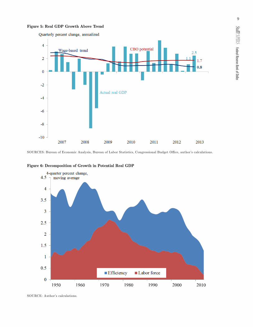
Recovery Speed. In Figure 5, I compare the pace of expansion of my wage-based measure of potentialoutput with that computed by the CBO and the path of growth in real GDP. The wage-based measureindicates a substantial slowdown in the pace of expansion of the economic potential since 2000. The way itis constructed naturally decomposes growth in potential real output into two factors: growth of the laborforce and improvements in effi ciency.

As shown in Figure 6, both slower growth in economic effi ciency and a slowdown in the growth rate of thelabor force contribute to the slowdown in potential growth. The reduction in the labor force participationrate started more than a decade ago, is currently accelerating largely due to early retirement of baby boomers(see Hornstein and Rhodes 2013), and is expected to last for another two decades due to demographic factors,as shown in Szafran (2002) and many others. The slight reduction in the pace of improvement of economiceffi ciency may reflect the diffi culties this adjustment process imposes on the aging labor force. A similaradjustment process was under way in the late 1970s and early 1980s when the entrance of baby boomersinto the labor force and increased participation of women led to a reduction in average economic effi ciency,as illustrated in Figure 4.

The gradual slowdown in trend implies that the speed of recovery from the last recession, that is, thespeed of growth net of trend, has been 1.3 percent per year – not stellar, but much higher than the speedone could infer from the estimates of the CBO. As shown in Table 1, this pace is similar to many pastrecessions, in fact not far behind compared with the average pace of recovery from all seven recessions inthe sample.

6The difference of my measure with the CBO’s estimate has two main sources. First, the CBO assumes a slower declinein labor force participation than has been observed. Second, the CBO assumes that this factor affects only the contribution oflabor to GDP growth, while my estimate (due to step 2) assumes that it affects all components of GDP equally.


Figure 5: Real GDP Growth Above Trend


Figure 6: Decomposition of Growth in Potential Real GDP

SOURCE: Author’s calculations.

10Sta

ffPAP

ERS

Fede

ral Re

serve

Bank

of Da

llas

Table 1: The Speed of Recovery in a Historical PerspectiveRecovery Average

Start Until recovery rate

1954:Q2 1956:Q4 1.611961:Q1 1963:Q3 1.531970:Q4 1973:Q2 2.121975:Q1 1977:Q3 2.251982:Q4 1985:Q2 2.081991:Q4 1994:Q2 1.592003:Q1 2005:Q3 1.01

Average of 7 recoveries 1.74

2009:Q3 2013:Q2 1.28


Inflation Pressures. A desirable feature of a good measure of the output gap is its ability to forecastinflation pressures. To assess whether my wage-based measure is useful for forecasting inflation, I follow themethodology of Koenig and Atkinson (2012) and use the twelve-month Trimmed Mean PCE inflation rateas a measure of inflation because it is relatively less volatile compared with headline inflation and gives agood proxy of underlying current and future inflation pressures. By splitting the period of available datasince 1985 in two parts at the turn of the century, I delineate the first period for estimating a forecastingrelationship and the second period for assessing out-of-sample forecast performance.

I estimate a relationship between the current inflation rate, πt, net of the Survey of Professional Fore-casters (SPF) long-forward inflation expectations, πLFt , and a four-quarter lag of inflation. Key explanatoryvariables include the level of the output gap, xt, and the four-quarter change in the output gap:

πt − πLFt = α+ β(πt−4 − πLFt−4

)+ γxt−4 + δ (xt−4 − xt−8) (8)

The results of the forecasting exercise using various measures of the output gap are presented in Table2. These results show that (the one-quarter change in) the wage-based measure performs at least as well asusing (the three-quarter change in) the unemployment rate. It does much better than most other commonlyused measures of the output gap, both in-sample and out-of-sample. A hybrid model, which combines thelevel of a wage-based output gap and a thre-quarter change in unemployment, cannot improve upon thewage-based measure although it combines the most useful information from both series. Figure 7 illustratesthe out-of-sample fit of forecasts of inflation produced using the wage-based measure of the output gap.

However, note that inflation forecasting is far from being the primary objective behind the developmentof my measure of the output gap. Thus, this forecasting exercise serves as a simple check of consistencywith economic intuition, and the results of the exercise are purely suggestive. There remain a large numberof caveats related to the choice of time period, measure of inflation, additional explanatory variables, andthe non-real-time nature of the forecast.

In this section, I have demonstrated that my measure of the output gap satisfies two most commonlyheld economic beliefs regarding the business-cycle properties of the output gap. First, the wage-basedmeasure is consistent with Okun’s law, both in differences and in levels. Second, the wage-based measure isconsistent with the “natural rate”version of the Phillips curve helpful in forecasting price pressures. Theseare two necessary economic conditions that turn a measure into a useful tool for guiding policymaking. Moreimportant, in the next section, I discuss the statistical properties of my measure that make it convenientfrom a practical standpoint.


Figure 7: Output Gap Useful for Year-Ahead Inflation Forecasts

SOURCES: Bureau of Economic Analysis, Bureau of Labor Statistics, Federal Reserve Bank of Dallas, author’s calculations.

Table 2: Forecasting Performance of Different Measures of the Output GapStandard error

Gap measure Fitted Forecast

None 0.293 0.479CBO potential 0.246 0.445Hodrick-Prescott filter 0.251 0.418Unemployment level 0.243 0.386Wage-based measure 0.246 0.328Hybrid model 0.242 0.350

SOURCES: Bureau of Economic Analysis, Bureau of Labor Statistics, Congressional Budget Offi ce, Federal Reserve Bank of

Dallas, author’s calculations.

4. STATISTICAL PROPERTIESOrphanides and van Norden (2002) identify updates to parameter estimates due to new data releases

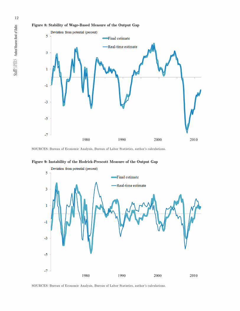
as the most serious problem underlying the unreliability of end-of-sample estimates of the output gap forexisting measures of the output gap. They argue that this property makes the majority of existing measuresunsuitable for real-time policy analysis. In this section, I demonstrate that, unlike other measures, mymeasure does not “wiggle its tail.”

To demonstrate that, I compute the estimates of the output gap that my method would have producedbased on data available at earlier points in time. I compare the real-time estimates of the output gap with“final”estimates, that is, estimates computed as of 2013, in Figure 8. Figure 8 demonstrates that there isvirtually no difference between the final estimates and the real-time estimates of the output gap.

Figure 9 shows a comparison of real-time and final estimates of the output gap using the Hodrick-Prescott filter. The stark contrast between the two figures demonstrates that my real-time estimates ofthe output gap are an order of magnitude more robust to new data releases than those produced by theHP-filter or the band-pass filter. As mentioned earlier, Orphanides and van Norden’s estimates imply thatamong the variety of aggregate methods, based either on the univariate or the multivariate approach, theHP-filter has nearly the lowest root mean square error (RMSE) due to new data releases. This implies thatmy method outperforms by an order of magnitude all of the methods in terms of real-time robustness.

12Sta

ffPAP

ERS

Fede

ral Re

serve

Bank

of Da

llas

Figure 8: Stability of Wage-Based Measure of the Output Gap


Figure 9: Instability of the Hodrick-Prescott Measure of the Output Gap



Figure 10: Uncertainty of Output Gap Measures Fades When New Data Are Released

SOURCE: Author’s calculations.

Figure 11: Output Gap Measure Robust to Shifts in Labor Share and Hours per Worker

SOURCES: Bureau of Labor Statistics, author’s calculations.

14Sta

ffPAP

ERS

Fede

ral Re

serve

Bank

of Da

llas

To further illustrate this point I compute the RMSE of the output gap as a function of the time lagbetween the current period (that is, the period for which the latest data are available) and the period forwhich the output gap is estimated. I average these errors for all current periods starting with 1971 (allowingan initial period to initialize the estimation and fix the normalization). Figure 10 plots the RMSE as afunction of the time lag for the HP-filter, the band-pass filter, and for my wage-based measure of the outputgap. It shows that it takes at most three quarters for my measure to stabilize around the final estimate,with the real-time error on the order of 0.2 percent. However, the average real-time error in the output gapproduced by the HP-filter starts at 1.5 percent and takes more than three years to stabilize. Moreover, it isnot until almost a decade later that the HP-filter becomes as robust as my wage-based real-time estimateof the output gap.

Robustness Analysis. I also briefly discuss the robustness of my estimates to the assumptions regardinglong-run stability of hours per worker and the labor shares. For robustness analysis I generate an artificialdata series for hours worked, which are by construction constant fractions of employment. Similarly, Igenerate an artificial data series for labor compensation, which is assumed to be a constant fraction of GDP.In each case, I replace the actual data by the artificial data series and re-compute my estimate of the outputgap. The difference between the baseline estimate of the output gap and the estimates based on artificialdata gives a perfect estimate of the error that might be introduced by using the assumptions. Figure 11compares all three estimates. It shows that the standard error of each of the assumptions does not exceedhalf a percentage point. The estimate of the standard error introduced by both of these assumptions jointlyis 0.51 percent.

5. CONCLUSIONMy wage-based measure of the output gap both satisfies basic economic intuition and remains virtually

unchanged when new data are released. It is highly robust to deviations from the underlying assumptionsemployed in its construction. This makes the wage-based measure of the output gap a reliable tool forunderstanding current economic conditions and guiding policymaking. The methodology may also proveuseful in academic research for detrending GDP and other macroeconomic time series, both for the U.S.and other countries.

However, caution must be expressed regarding data revisions, which may lead to sizable changes in theestimate of the output gap. For instance, the 2013 revision of national accounts going all the way back to1929 resulted in a 1 percent upward revision of the output gap. This change translated one-to-one fromthe revision of the path of real GDP. Unfortunately, no method of constructing the output gap can insulatefrom such data revisions.

REFERENCESBeveridge, Stephen, and Charles R. Nelson (1981), “A New Approach to Decomposition of Economic Time

Series Into Permanent and Transitory Components With Particular Attention to Measurement of theBusiness Cycle,”Journal of Monetary Economics, 7: 151-74.

Christiano, Lawrence J., and Terry J. Fitzgerald (2003), “The Band Pass Filter, ” International EconomicReview, 44(2): 435-65.

Clark, Peter K. (1987), “The Cyclical Component of U.S. Economic Activity,”The Quarterly Journal ofEconomics, 102(4): 797-814.

Farmer, Roger E.A. (2008), “Old Keynesian Economics,”Chapter 2 in Macroeconomics in the Small andthe Large: Essays on Microfoundations, Macroeconomic Applications and Economic History in Honorof Axel Leijonhufvud (Cheltenham, UK: Edward Elgar), 23-43.

Hodrick, Robert J., and Edward C. Prescott (1997), “Postwar U.S. Business Cycles: An Empirical Investi-gation,”Journal of Money, Credit and Banking, 29(1): 1-16.

Hornstein, Andreas, and Karl Rhodes (2013), “Will a Surge in Labor Force Participation Impede Unem-ployment Rate Improvement?”Federal Reserve Bank of Richmond, Economic Brief 13-08, August.

Keynes, John Maynard (1936), The General Theory of Employment, Interest, and Money, (Repr. London:Macmillan, 2007).

Kiley, Michael T. (2013) “Output Gaps,”Journal of Macroeconomics, 37(C): 1-18.

Koenig, Evan F., and Tyler Atkinson (2012), “Inflation, Slack, and Fed Credibility,”Federal Reserve Bankof Dallas Staff Papers, no. 16.


Kuttner, Kenneth N. (1994), “Estimating Potential Output as a Latent Variable,”Journal of Business &Economic Statistics, 12(3): 361-68.

Laubach, Thomas, and John C. Williams (2003), “Measuring the Natural Rate of Interest,”The Review ofEconomics and Statistics, 85(4): 1063-70.

Mishkin, Frederic S. (2007), “Estimating Potential Output,”(Speech at the Conference on Price Measure-ment for Monetary Policy), Federal Reserve Bank of Dallas, May 24.

Okun, Arthur M. (1962), “Potential GNP, Its Measurement and Significance,”Proceedings of the Businessand Economics Statistics Section, American Statistical Association, 98-104.

Orphanides, Athanasios, and Simon van Norden (2002), “The Unreliability of Output-Gap Estimates inReal Time,”The Review of Economics and Statistics, 84(4): 569-83.

Plotnikov, Dmitry (2012), “Hysteresis in Unemployment and Jobless Recoveries,”unpublished paper.

Szafran, Robert F. (2002), “Age-Adjusted Labor Force Participation Rates, 1960-2045,”Monthly LaborReview, Bureau of Labor Statistics, September, 25-38.

Documents

Staff Papers - Dallas Fed