Staggered and In-line Submerged Jet Arrays for Power Electronics Using Variable Area

Discharge Manifolds

by

Michael Andrew Henry

A thesis submitted to the Graduate Faculty of

Auburn University

in partial fulfillment of the

requirements for the Degree of

Master of Science

Auburn, Alabama

August 4, 2018

Keywords: jet impingement, single-phase, spent flow management,

local heat transfer coefficient measurement, water-ethylene glycol, staggered arrays

Copyright 2018 by Michael Andrew Henry

Approved by

Sushil H. Bhavnani, Co-Chair, Professor of Mechanical Engineering

Roy W. Knight, Co-Chair, Associate Professor of Mechanical Engineering

Daniel K. Harris, Associate Professor of Mechanical Engineering

ii

Abstract

Power electronics packages in electric and hybrid vehicles require dedicated and

dynamic cooling to perform reliably. Generally, such packages are designed to spread heat to a

large surface area, and employing the radiator flow loop and fluid to provide a more aggressive,

liquid-cooling approach to supplement heat spreaders is an appealing idea when considering

cost, design, and fabrication. An array of liquid jets is the best single-phase cooling technique for

cooling large surfaces. The highest regions of cooling in an array of jets are located at the

stagnation points and, to a lesser degree, the fountain regions. One of the more significant issues

facing arrays of jets is the degradation of downstream jets caused by the interference of fluid

spent by upstream jets. The idea of an angled confining wall to divert the spent flow, and

therefore prevent the entrainment of flows, was complemented by investigations into the

viability of water-ethylene glycol as a working fluid and staggered arrays. A measurement

technique was used to determine the local thermal characteristics for cases of varying jet

Reynolds number, plate angle, jet-to-jet pitch, and jet-to-plate height above the surface. Water-

ethylene glycol and staggered arrays were compatible and showed improved heat transfer when

combined with the angled wall spent fluid management scheme.

iii

Acknowledgements

Thanks go to the members of my advisory committee, Dr. Sushil H. Bhavnani, Dr. Roy W.

Knight, and Dr. Daniel K. Harris, for serving upon it. Dr. Bhavnani and Dr. Knight warrant special

thanks for the counsel and guidance they’ve provided in the course of this study.

Thanks go to Dr. John F. Maddox for laying the foundations of this project, and for serving

in an auxiliary role for troubleshooting technical issues and tailoring their solutions.

Thanks go to Kayla and Sriram for rounding out a triumvirate, serving as colleagues in

times of both academic perseverance and shared comradery.

Finally, thanks go to my mother, father, brother, sister, and grandmother, who were

essential throughout this work, and without whom all the steps beforehand would have been

impossible.

iv

Table of Contents

Abstract . . . . . . . . . . . . . . . . . . . . . . . . . . . . . . . . . . . . . . . . . . . . . . . . . . . . . . . . . . . . . . . . . . . . . . ii

Acknowledgements . . . . . . . . . . . . . . . . . . . . . . . . . . . . . . . . . . . . . . . . . . . . . . . . . . . . . . . . . . . . iii

List of Figures . . . . . . . . . . . . . . . . . . . . . . . . . . . . . . . . . . . . . . . . . . . . . . . . . . . . . . . . . . . . . . . . .vii

List of Tables . . . . . . . . . . . . . . . . . . . . . . . . . . . . . . . . . . . . . . . . . . . . . . . . . . . . . . . . . . . . . . . . . x

Nomenclature . . . . . . . . . . . . . . . . . . . . . . . . . . . . . . . . . . . . . . . . . . . . . . . . . . . . . . . . . . . . . . . . . xi

1 Introduction and Theory . . . . . . . . . . . . . . . . . . . . . . . . . . . . . . . . . . . . . . . . . . . . . . . . . . . 1

1.1 Electronics Thermal Management Considerations . . . . . . . . . . . . . . . . . . . . . . . . 1

1.2 Applicability of Power Electronics Cooling Techniques . . . . . . . . . . . . . . . . . . . . 3

1.3 Jet Theory . . . . . . . . . . . . . . . . . . . . . . . . . . . . . . . . . . . . . . . . . . . . . . . . . . . . . . . . 4

1.3.1 Jet Regions . . . . . . . . . . . . . . . . . . . . . . . . . . . . . . . . . . . . . . . . . . . . . . . . . 5

2 Literature Review . . . . . . . . . . . . . . . . . . . . . . . . . . . . . . . . . . . . . . . . . . . . . . . . . . . . . . . . 7

v

3 Experimental Setup and Procedures . . . . . . . . . . . . . . . . . . . . . . . . . . . . . . . . . . . . . . . . . 14

3.1 Jet Plates . . . . . . . . . . . . . . . . . . . . . . . . . . . . . . . . . . . . . . . . . . . . . . . . . . . . . . . . 14

3.2 Flow Chamber and Heat Generation . . . . . . . . . . . . . . . . . . . . . . . . . . . . . . . . . . 17

3.3 Flow Loop . . . . . . . . . . . . . . . . . . . . . . . . . . . . . . . . . . . . . . . . . . . . . . . . . . . . . . . 19

3.4 Local and Average Surface Measurements . . . . . . . . . . . . . . . . . . . . . . . . . . . . . 21

4 Results . . . . . . . . . . . . . . . . . . . . . . . . . . . . . . . . . . . . . . . . . . . . . . . . . . . . . . . . . . . . . . . . 25

4.1 Overview of Parameters Tested . . . . . . . . . . . . . . . . . . . . . . . . . . . . . . . . . . . . . . . 25

4.1.1 Water-Ethylene Glycol Tests . . . . . . . . . . . . . . . . . . . . . . . . . . . . . . . . . . 25

4.1.2 Staggered Array Tests . . . . . . . . . . . . . . . . . . . . . . . . . . . . . . . . . . . . . . . .26

4.2 Water-Ethylene Glycol Results and Discussion . . . . . . . . . . . . . . . . . . . . . . . . . . 29

4.3 Staggered Array Results and Discussion . . . . . . . . . . . . . . . . . . . . . . . . . . . . . . . . 33

4.4 Numerical Comparison . . . . . . . . . . . . . . . . . . . . . . . . . . . . . . . . . . . . . . . . . . . . . 39

5 Conclusion . . . . . . . . . . . . . . . . . . . . . . . . . . . . . . . . . . . . . . . . . . . . . . . . . . . . . . . . . . . . . 42

5.1 Suggestions for Future Work . . . . . . . . . . . . . . . . . . . . . . . . . . . . . . . . . . . . . . . . . 44

Bibliography . . . . . . . . . . . . . . . . . . . . . . . . . . . . . . . . . . . . . . . . . . . . . . . . . . . . . . . . . . . . . . . . . 46

Appendices . . . . . . . . . . . . . . . . . . . . . . . . . . . . . . . . . . . . . . . . . . . . . . . . . . . . . . . . . . . . . . . . . . 50

vi

A Data Acquisition . . . . . . . . . . . . . . . . . . . . . . . . . . . . . . . . . . . . . . . . . . . . . . . . . . . . . . . . 50

A.1 Procedure . . . . . . . . . . . . . . . . . . . . . . . . . . . . . . . . . . . . . . . . . . . . . . . . . . . . . . . . 50

A.1.1 Opening the Flow Chamber. . . . . . . . . . . . . . . . . . . . . . . . . . . . . . . . . . . . . 50

A.1.2 Closing the Flow Chamber . . . . . . . . . . . . . . . . . . . . . . . . . . . . . . . . . . . . . 51

A.1.3 Replacing the Jet Plate . . . . . . . . . . . . . . . . . . . . . . . . . . . . . . . . . . . . . . . . . 51

A.1.4 Translating in the x-direction . . . . . . . . . . . . . . . . . . . . . . . . . . . . . . . . . . . . 52

A.1.5 Translating in the y-direction. . . . . . . . . . . . . . . . . . . . . . . . . . . . . . . . . . . . 53

A.1.6 Changing the Height of the Jet Plate . . . . . . . . . . . . . . . . . . . . . . . . . . . . . . 53

A.1.7 Initializing the System . . . . . . . . . . . . . . . . . . . . . . . . . . . . . . . . . . . . . . . . . 54

A.2 Considerations for Potential Revisions to the Test Chamber Design . . . . . . . . . . 54

B Data Reduction . . . . . . . . . . . . . . . . . . . . . . . . . . . . . . . . . . . . . . . . . . . . . . . . . . . . . . . . . 57

B.1 Calculating Local Surface Values . . . . . . . . . . . . . . . . . . . . . . . . . . . . . . . . . . . . . . . . 57

B.2 Calculating Average Surface Values . . . . . . . . . . . . . . . . . . . . . . . . . . . . . . . . . . . . . 63

C Experimental Uncertainty Analysis . . . . . . . . . . . . . . . . . . . . . . . . . . . . . . . . . . . . . . . . . . 69

C.1 Determining Thermocouple Uncertainty Using Sequential Perturbations . . . . . . . . . 69

C.2 Local Surface Measurement Uncertainties . . . . . . . . . . . . . . . . . . . . . . . . . . . . . . . . . 71

vii

C.3 Surface Average Measurement Uncertainties . . . . . . . . . . . . . . . . . . . . . . . . . . . . . . . 72

D Experimental Results . . . . . . . . . . . . . . . . . . . . . . . . . . . . . . . . . . . . . . . . . . . . . . . . . . . . . 73

D.1 Experimental Data Summary . . . . . . . . . . . . . . . . . . . . . . . . . . . . . . . . . . . . . . . . . . . .73

D.2 Experimental Surface Maps . . . . . . . . . . . . . . . . . . . . . . . . . . . . . . . . . . . . . . . . . . . . 75

viii

List of Figures

IGBT module . . . . . . . . . . . . . . . . . . . . . . . . . . . . . . . . . . . . . . . . . . . . . . . . . . . . . . . . . . . . . . . . . 2

Overheated module . . . . . . . . . . . . . . . . . . . . . . . . . . . . . . . . . . . . . . . . . . . . . . . . . . . . . . . . . . . . . 3

Types of jets . . . . . . . . . . . . . . . . . . . . . . . . . . . . . . . . . . . . . . . . . . . . . . . . . . . . . . . . . . . . . . . . . . 5

Regions of impinging jets . . . . . . . . . . . . . . . . . . . . . . . . . . . . . . . . . . . . . . . . . . . . . . . . . . . . . . . . 6

Rholfs et. al. [14] thermochromatic liquid crystals. . . . . . . . . . . . . . . . . . . . . . . . . . . . . . . . . . . . . 8

Brunschwiler et. al. [9] flow geometry. . . . . . . . . . . . . . . . . . . . . . . . . . . . . . . . . . . . . . . . . . . . . . 9

Arens et. al. [22] jet arrays with and without variable diameter . . . . . . . . . . . . . . . . . . . . . . . . . . 10

3.1 Spatial arrangement jet array types . . . . . . . . . . . . . . . . . . . . . . . . . . . . . . . . . . . . . . . . . . 15

(a) Inline . . . . . . . . . . . . . . . . . . . . . . . . . . . . . . . . . . . . . . . . . . . . . . . . . . . . . . . . . . . . . . 15

(b) Streamwise staggered . . . . . . . . . . . . . . . . . . . . . . . . . . . . . . . . . . . . . . . . . . . . . . . . . . 15

(c) Transverse staggered . . . . . . . . . . . . . . . . . . . . . . . . . . . . . . . . . . . . . . . . . . . . . . . . . . 16

3.2 Side view of the angled manifold region . . . . . . . . . . . . . . . . . . . . . . . . . . . . . . . . . . . . . . 16

3.3 Photograph of 3D-printed jet plates . . . . . . . . . . . . . . . . . . . . . . . . . . . . . . . . . . . . . . . . . . 17

ix

3.4 Cross section of experimental apparatus . . . . . . . . . . . . . . . . . . . . . . . . . . . . . . . . . . . . . . 18

3.5 Cross section of copper blocks . . . . . . . . . . . . . . . . . . . . . . . . . . . . . . . . . . . . . . . . . . . . . 19

3.6 Flow loop . . . . . . . . . . . . . . . . . . . . . . . . . . . . . . . . . . . . . . . . . . . . . . . . . . . . . . . . . . . . . . 20

3.7 Photograph of experimental apparatus . . . . . . . . . . . . . . . . . . . . . . . . . . . . . . . . . . . . . . . 21

3.8 Surface map locations . . . . . . . . . . . . . . . . . . . . . . . . . . . . . . . . . . . . . . . . . . . . . . . . . . . . 23

4.1 Varying patterns for staggered arrays . . . . . . . . . . . . . . . . . . . . . . . . . . . . . . . . . . . . . . . . 26

4.2 Surface maps of water-ethylene glycol at increasing flow rates . . . . . . . . . . . . . . . . . . . 29

4.3 Average heat transfer coefficients for water and water-ethylene glycol . . . . . . . . . . . . . 30

4.4 Average Nusselt numbers for water and water-ethylene glycol . . . . . . . . . . . . . . . . . . . . 31

4.5 Surface maps of water-ethylene glycol at increasing manifold angle . . . . . . . . . . . . . . . 32

4.6 Temperature rise surface maps for varying nozzle pattern . . . . . . . . . . . . . . . . . . . . . . . . 34

4.7 Average Nusselt numbers for varying angle and nozzle pattern . . . . . . . . . . . . . . . . . . . . 35

4.8 Surface maps of staggered plates at increasing angle . . . . . . . . . . . . . . . . . . . . . . . . . . . . 36

4.9 Nusselt numbers for varying angle and pitch using plates with the streamwise staggered

pattern . . . . . . . . . . . . . . . . . . . . . . . . . . . . . . . . . . . . . . . . . . . . . . . . . . . . . . . . . . . . . . . . 37

4.10 Nusselt numbers comparing test with pitch, 𝑃∗ = 3. . . . . . . . . . . . . . . . . . . . . . . . . . . . . 38

4.11 Comparison of numerical and experimental surface plots. . . . . . . . . . . . . . . . . . . . . . . . . 40

x

D.1 Water-ethylene glycol over increasing Reynolds numbers . . . . . . . . . . . . . . . . . . . . . . . . 76

D.2 Water-ethylene glycol over increasing manifold angle. . . . . . . . . . . . . . . . . . . . . . . . . . . 77

D.3 Water-ethylene glycol with 𝐻∗ = 1 and 2 . . . . . . . . . . . . . . . . . . . . . . . . . . . . . . . . . . . . .78

D.4 Streamwise staggered array with 𝑃∗ = 3 and increasing Reynolds number . . . . . . . . . . . 79

D.5 Streamwise staggered array with 𝑃∗ = 4 and increasing Reynolds number. . . . . . . . . . . 80

D.6 Streamwise staggered array with 𝑃∗ = 6 and increasing Reynolds number . . . . . . . . . . . 81

D.7 Transverse staggered array with 𝑃∗ = 6 and increasing Reynolds number . . . . . . . . . . . 82

D.8 Streamwise staggered arrays with increasing pitch. . . . . . . . . . . . . . . . . . . . . . . . . . . . . . 83

D.9 Streamwise staggered compared to transverse staggered . . . . . . . . . . . . . . . . . . . . . . . . . 84

D.10 Streamwise staggered increasing angle with 𝑃∗ = 4. . . . . . . . . . . . . . . . . . . . . . . . . . . . . 85

D.11 Streamwise staggered increasing angle with 𝑃∗ = 6. . . . . . . . . . . . . . . . . . . . . . . . . . . . . 86

D.12 Transverse staggered increasing angle with 𝑃∗ = 6 . . . . . . . . . . . . . . . . . . . . . . . . . . . . . 87

D.13: Streamwise staggered increasing Reynolds number with 𝛾 = 7.5° and 𝑃∗ = 6 . . . . . . . . 88

xi

List of Tables

2.1 Summary of relevant criteria for studies reviewed; liquid working fluid, single . . . . . . . .11

2.1 Summary of relevant criteria for studies reviewed; liquid working fluid, array . . . . . . . .12

2.1 Summary of relevant criteria for studies reviewed; gaseous working fluid . . . . . . . . . . . 13

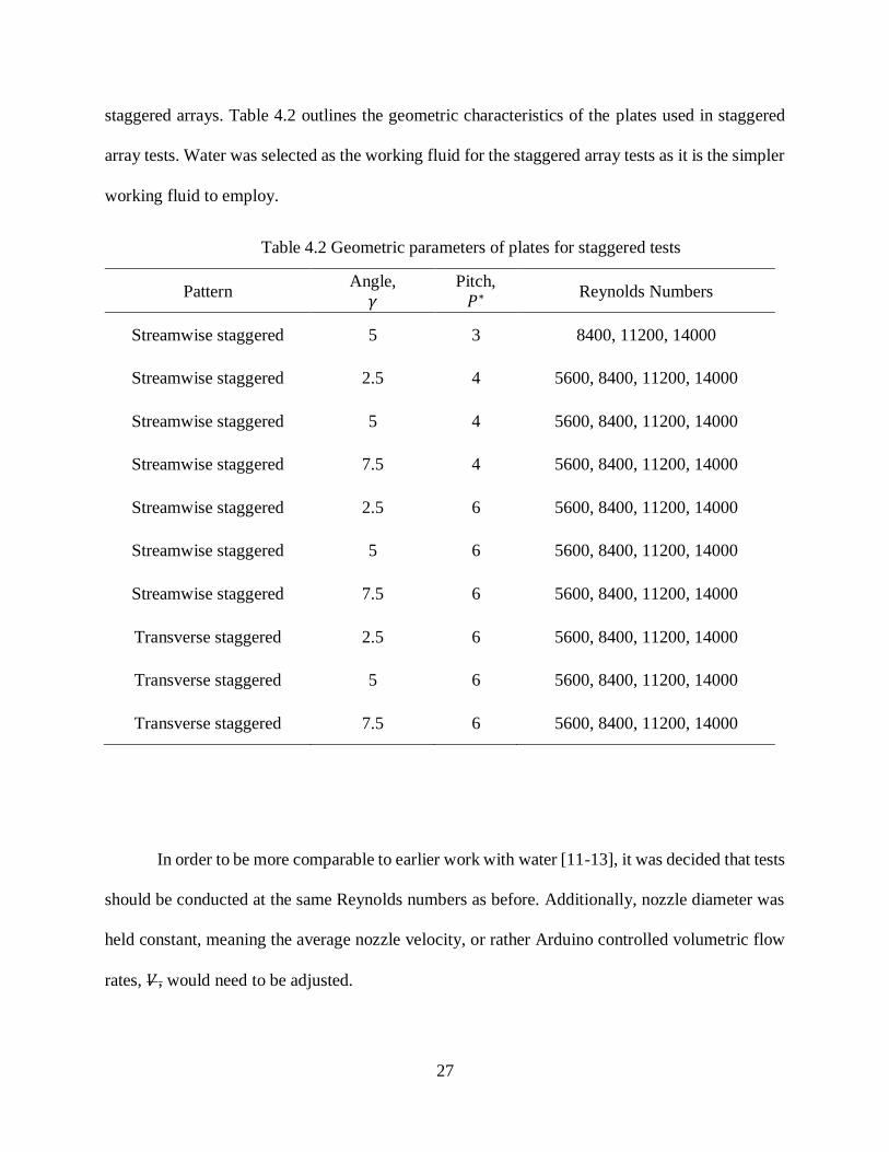
4.1 Geometric parameters of plates for water-ethylene glycol tests . . . . . . . . . . . . . . . . . . . . 26

4.2 Geometric parameters of plates for staggered tests . . . . . . . . . . . . . . . . . . . . . . . . . . . . . 27

4.3 Volumetric flow rates used in testing staggered arrays . . . . . . . . . . . . . . . . . . . . . . . . . . . 28

4.4 Varying heights: water compared to WEG . . . . . . . . . . . . . . . . . . . . . . . . . . . . . . . . . . . . 32

4.5 Geometries and results for select papers. . . . . . . . . . . . . . . . . . . . . . . . . . . . . . . . . . . . . . 39

B.1 Sample temperature data . . . . . . . . . . . . . . . . . . . . . . . . . . . . . . . . . . . . . . . . . . . . . . . . . . 57

B.2 Individual and average temperature values . . . . . . . . . . . . . . . . . . . . . . . . . . . . . . . . . . . 59

B.3 Thermal conductivity of water-ethylene glycol chart . . . . . . . . . . . . . . . . . . . . . . . . . . . . 62

B.4 Calculated local surface values . . . . . . . . . . . . . . . . . . . . . . . . . . . . . . . . . . . . . . . . . . . . . 63

B.5 Sample average surface value data, streamwise staggered, water . . . . . . . . . . . . . . . . . . 64

xii

B.6 Estimated local surface values . . . . . . . . . . . . . . . . . . . . . . . . . . . . . . . . . . . . . . . . . . . . . . 64

D.1 Summary of experimental data . . . . . . . . . . . . . . . . . . . . . . . . . . . . . . . . . . . . . . . . . . . . . 73

Nomenclature

Acronyms

IGBT insulated-gate bipolar transistor

MOSFET metal-oxide-semiconductor field-effect transistor

PID proportional-integral-derivative

VFD variable frequency drive

WEG water-ethylene glycol

English Letter Symbols

𝐴𝑛 flow area of a nozzle, m2

𝐷ℎ hydraulic diameter, m

xiii

𝐷𝑛 nozzle diameter, m

𝐻 height of nozzles above surface, m

ℎ local heat transfer coefficient, W/(m2 · K)

ℎ̅ mean heat transfer coefficient, W/(m2 · K)

𝑘 thermal conductivity, W/(m · K)

𝐿𝑛 nozzle length, m

𝑁 number of nozzles

𝑁𝑢𝐷𝑛 local jet Nusselt number

𝑁𝑢̅̅ ̅̅ 𝐷𝑛 mean jet Nusselt number

𝑃 pitch between nozzles, m

𝑞′′ heat flux, W/m2

𝑅𝑒𝐷𝑛 jet Reynolds number

𝑈𝑛 average nozzle velocity, m

𝑉 volumetric flow rate, L/s

𝑥 horizontal distance in flow direction from center, m

xiv

𝑦

horizontal distance perpendicular to flow direction from center jet,

m

𝑧 vertical distance above impingement surface, m

Greek Letter Symbols

𝛾 angle between plate and surface

𝜈 kinematic viscosity, m2/s

Superscripts

* nondimensionalized with respect to 𝐷𝑛

Subscripts

𝑛 nozzle

1

Chapter 1

Introduction and Theory

1.1 Electronics Thermal Management Considerations

Modern electronics continue to increase in power output and decrease in size, causing a need

for cooling strategies more efficient at heat removal and implemented in more proportionate

sizes. Traditional air-cooling techniques are not capable of meeting the need, and more

aggressive and innovative cooling techniques are being explored, many focusing on liquid

cooling. In addition to the key factors of effectiveness and size, considerations must be made

with respect to cost, practicality, and reliability.

As thermal management systems tend to serve in auxiliary capacities to enable the reliable

use of electronics packages, the general cost and production volume expected for the core product

must be considered. For the purposes of a special case or limited market design, the cost associated

with the implementation of a given thermal management system is a more negotiable subject;

however, these solutions are also needed to address consumer products that operate on a broader

market, most notably in the automotive and consumer electronics industries. If a thermal

management scheme adds a significant enough portion to the total product cost, then it is not an

economic option for high volume production. When applying a revision to a portion of an existing

product, the ability for the new strategy to interface with the existing system must be taken under

consideration. Relative size, weight, and complexity not appropriately corresponding to the

existing structure can severely inhibit the ability of a system to perform the intended function.

2

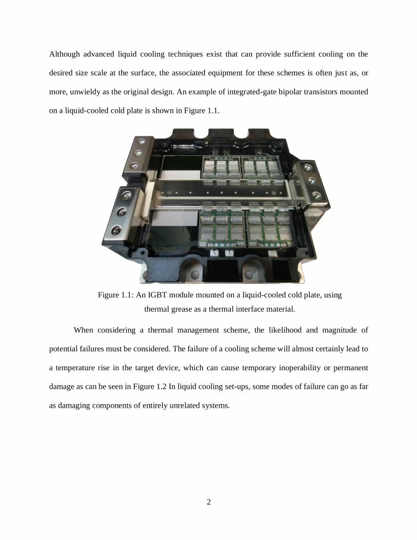
Although advanced liquid cooling techniques exist that can provide sufficient cooling on the

desired size scale at the surface, the associated equipment for these schemes is often just as, or

more, unwieldy as the original design. An example of integrated-gate bipolar transistors mounted

on a liquid-cooled cold plate is shown in Figure 1.1.

When considering a thermal management scheme, the likelihood and magnitude of

potential failures must be considered. The failure of a cooling scheme will almost certainly lead to

a temperature rise in the target device, which can cause temporary inoperability or permanent

damage as can be seen in Figure 1.2 In liquid cooling set-ups, some modes of failure can go as far

as damaging components of entirely unrelated systems.

Figure 1.1: An IGBT module mounted on a liquid-cooled cold plate, using

thermal grease as a thermal interface material.

3

1.2 Applicability of Power Electronics Cooling Techniques in Automotives

Preferred forms of electronics cooling techniques include the employment of two-phase

systems, microchannels, and jet impingement. Each of these is characterized by a solid surface

rejecting heat into a fluid, and the fluid being removed after receiving excess heat. Two-phase

cooling can achieve the highest values of heat transfer coefficient compared to the other

techniques, but will typically requires operation in settings with a high degree of environmental

control or high capacity cooling in the fluid loop. Microchannels are highly effective on small

scales, but require high amounts of pumping power and are costly to manufacture, although

additive manufacturing methods are poised to alleviate production costs. Jet impingement can be

effective on larger scales than microchannels, but include an inherent non-uniformity to the

cooling flow. This will be discussed more in the Chapter 2 literature review.

The electronics being used on board modern electric, hybrid-electric, and military vehicles

are no exception to the need for enhanced cooling strategies. Due to the large amounts of heat

produced under hood and the outdoor nature of the application, any system employed needs to be

Figure 1.2: IGBT module before (left) and after (right) overheating during operation due to

issues with containing the grease interface.

4

operable on wide ranges of temperature and relative humidity, making two-phase cooling an

unreliable choice [1-6]. Some success has been found in laboratory settings by Aranzabal [7], but

using R-134a as the working fluid drives up the cost and is prohibited in certain countries,

including the United States. The high cost of manufacturing microchannels would drive the

product price well above the range that would be acceptable for potential buyers. Jet impingement

is operable in a wide range of conditions, and relatively inexpensive to manufacture.

Furthermore, it would be preferable to make use of the resources already on hand within a

vehicle, and both two-phase cooling and microchannels would require a significant amount of

retrofitting to provide the infrastructure, i.e. condensers, pumps, etc., necessary to operate a flow

loop incorporating either cooling plan. The working fluid already conveniently flowing through

the existing flow loop is water-ethylene glycol (WEG), and is favored for its primary use for its

unlikeliness to change phase. High viscosity fluids like WEG require greater pumping power to

achieve the same flow characteristics as more typical electronics coolants, and place a higher

emphasis on the weak point of microchannels. Jet impingement provides a cooling option that is

compatible with the equipment and fluid on hand, is not as hindered by the viscous working fluid,

and with an effective fluid management scheme the non-uniform cooling can be mitigated.

1.3 Jet Theory

Jets are streams of directed fluid, often forced through an aperture and directed at a solid

surface either orthogonally (normal jets) or at an angle (oblique). If the aperture is through a thin,

flat wall it is called an orifice and the jet exits with a relatively flat velocity profile and poor heat

transfer characteristics. If the aperture is through a thicker wall, and turbulent flow is not induced,

the exit velocity profile takes on the parabolic shape of pipe flow with good heat transfer properties

5

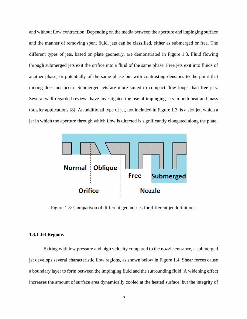
and without flow contraction. Depending on the media between the aperture and impinging surface

and the manner of removing spent fluid, jets can be classified, either as submerged or free. The

different types of jets, based on plate geometry, are demonstrated in Figure 1.3. Fluid flowing

through submerged jets exit the orifice into a fluid of the same phase. Free jets exit into fluids of

another phase, or potentially of the same phase but with contrasting densities to the point that

mixing does not occur. Submerged jets are more suited to compact flow loops than free jets.

Several well-regarded reviews have investigated the use of impinging jets in both heat and mass

transfer applications [8]. An additional type of jet, not included in Figure 1.3, is a slot jet, which a

jet in which the aperture through which flow is directed is significantly elongated along the plate.

1.3.1 Jet Regions

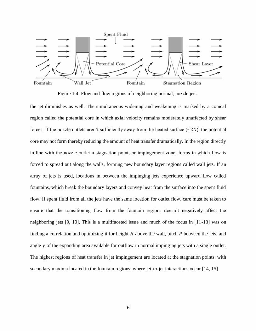
Exiting with low pressure and high velocity compared to the nozzle entrance, a submerged

jet develops several characteristic flow regions, as shown below in Figure 1.4. Shear forces cause

a boundary layer to form between the impinging fluid and the surrounding fluid. A widening effect

increases the amount of surface area dynamically cooled at the heated surface, but the integrity of

Figure 1.3: Comparison of different geometries for different jet definitions

6

the jet diminishes as well. The simultaneous widening and weakening is marked by a conical

region called the potential core in which axial velocity remains moderately unaffected by shear

forces. If the nozzle outlets aren’t sufficiently away from the heated surface (~2𝐷), the potential

core may not form thereby reducing the amount of heat transfer dramatically. In the region directly

in line with the nozzle outlet a stagnation point, or impingement zone, forms in which flow is

forced to spread out along the walls, forming new boundary layer regions called wall jets. If an

array of jets is used, locations in between the impinging jets experience upward flow called

fountains, which break the boundary layers and convey heat from the surface into the spent fluid

flow. If spent fluid from all the jets have the same location for outlet flow, care must be taken to

ensure that the transitioning flow from the fountain regions doesn’t negatively affect the

neighboring jets [9, 10]. This is a multifaceted issue and much of the focus in [11-13] was on

finding a correlation and optimizing it for height 𝐻 above the wall, pitch 𝑃 between the jets, and

angle 𝛾 of the expanding area available for outflow in normal impinging jets with a single outlet.

The highest regions of heat transfer in jet impingement are located at the stagnation points, with

secondary maxima located in the fountain regions, where jet-to-jet interactions occur [14, 15].

Figure 1.4: Flow and flow regions of neighboring normal, nozzle jets.

7

Chapter 2

Literature Review

As discussed in Chapter 1, the 2016 annual report of the National Renewable Energy

Laboratory’s Gilbert Moreno [1] supports the idea that the growth of under-hood sensor and

computer technologies considered standard in the automotive industry, in both commercial and

military applications, has generated a need for a rugged system for cooling electronics modules

that produce high amounts of heat. Air-cooling is unlikely to be able to provide an adequate amount

of cooling, therefore liquid-cooling options are typically considered and often employ water as the

working fluid. General information about the works reviewed is tabulated at the end of the chapter.

Jet impingement cooling is more suitable to automotive applications than two-phase

cooling and microchannels due to its low pressure drop and high volumetric flow rate, as well as

the wide range of ambient operating conditions that could be expected [2-6]. The primary

drawback with jet impingement arrays is the degradation of downstream jets by the exiting flow

of the upstream jets [9, 10] as flow from fountain regions are drawn toward an outlet.

Consequently, when using an array of jets, strategies for spent fluid management are often

considered. This thesis directly expands on one of these in the work of Maddox [11-13] which

involves the experimental and numerical investigation of an angled outlet manifold.

There are research groups exploring jet impingement that are not looking explicitly at spent

fluid management [4, 5, 8, 14-26], because the application or interest of their study only calls for

8

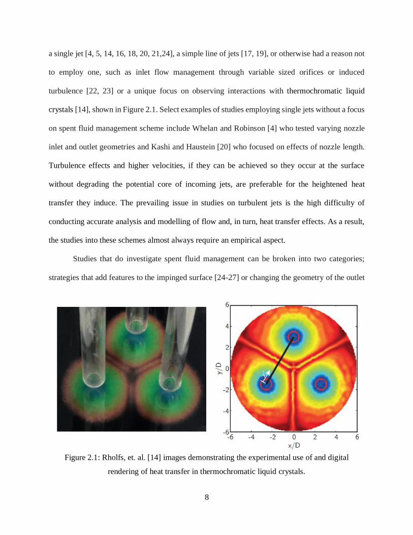
a single jet [4, 5, 14, 16, 18, 20, 21,24], a simple line of jets [17, 19], or otherwise had a reason not

to employ one, such as inlet flow management through variable sized orifices or induced

turbulence [22, 23] or a unique focus on observing interactions with thermochromatic liquid

crystals [14], shown in Figure 2.1. Select examples of studies employing single jets without a focus

on spent fluid management scheme include Whelan and Robinson [4] who tested varying nozzle

inlet and outlet geometries and Kashi and Haustein [20] who focused on effects of nozzle length.

Turbulence effects and higher velocities, if they can be achieved so they occur at the surface

without degrading the potential core of incoming jets, are preferable for the heightened heat

transfer they induce. The prevailing issue in studies on turbulent jets is the high difficulty of

conducting accurate analysis and modelling of flow and, in turn, heat transfer effects. As a result,

the studies into these schemes almost always require an empirical aspect.

Studies that do investigate spent fluid management can be broken into two categories;

strategies that add features to the impinged surface [24-27] or changing the geometry of the outlet

Figure 2.1: Rholfs, et. al. [14] images demonstrating the experimental use of and digital

rendering of heat transfer in thermochromatic liquid crystals.

9

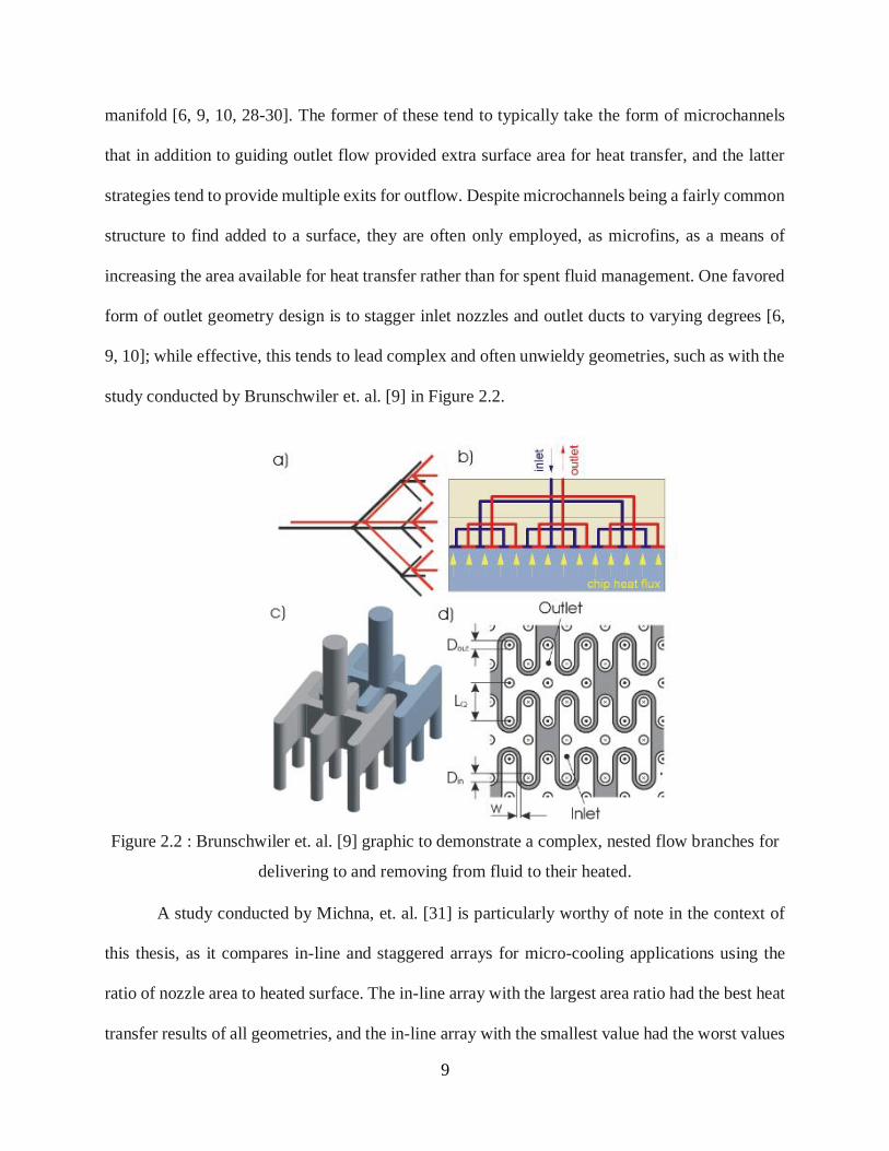
manifold [6, 9, 10, 28-30]. The former of these tend to typically take the form of microchannels

that in addition to guiding outlet flow provided extra surface area for heat transfer, and the latter

strategies tend to provide multiple exits for outflow. Despite microchannels being a fairly common

structure to find added to a surface, they are often only employed, as microfins, as a means of

increasing the area available for heat transfer rather than for spent fluid management. One favored

form of outlet geometry design is to stagger inlet nozzles and outlet ducts to varying degrees [6,

9, 10]; while effective, this tends to lead complex and often unwieldy geometries, such as with the

study conducted by Brunschwiler et. al. [9] in Figure 2.2.

Figure 2.2 : Brunschwiler et. al. [9] graphic to demonstrate a complex, nested flow branches for

delivering to and removing from fluid to their heated.

A study conducted by Michna, et. al. [31] is particularly worthy of note in the context of

this thesis, as it compares in-line and staggered arrays for micro-cooling applications using the

ratio of nozzle area to heated surface. The in-line array with the largest area ratio had the best heat

transfer results of all geometries, and the in-line array with the smallest value had the worst values

10

of all geometries. Of the three staggered arrays, the median value of area ratio performed better

than the other two. Michna group noted this was probably due to negative crossflow effects as

there is no spent fluid management concept applied. It should also be considered that the jet-to-jet

spacing on the staggered array is so low that there is not enough space for fountain effects to

properly form. Average Nusselt numbers for water were between 5 and 80 for Reynolds numbers

between 50 and 3500.

The influence of reviewed literature on the water-ethylene glycol testing section of this

study is limited; however the work by Narumanchi et. al.[5] provides a few reference points for

validating certain parameters such as selected flow rates and jet-to-surface heights. Several of the

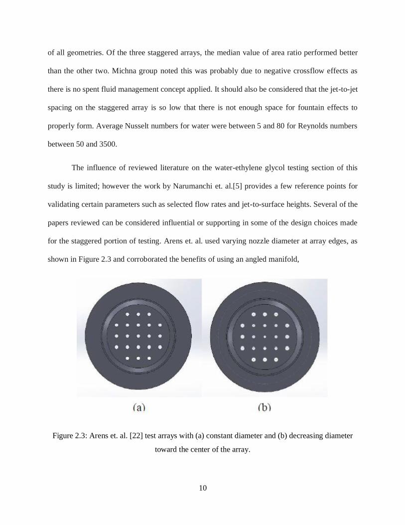
papers reviewed can be considered influential or supporting in some of the design choices made

for the staggered portion of testing. Arens et. al. used varying nozzle diameter at array edges, as

shown in Figure 2.3 and corroborated the benefits of using an angled manifold,

Figure 2.3: Arens et. al. [22] test arrays with (a) constant diameter and (b) decreasing diameter

toward the center of the array.

11

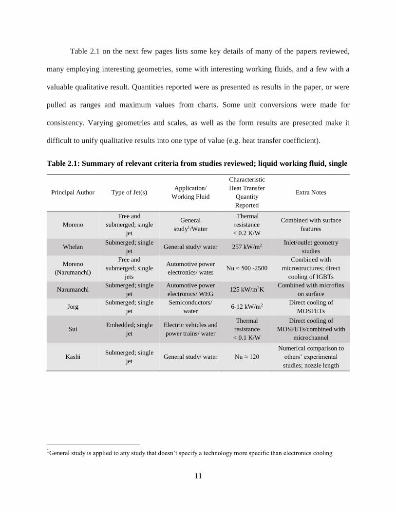
Table 2.1 on the next few pages lists some key details of many of the papers reviewed,

many employing interesting geometries, some with interesting working fluids, and a few with a

valuable qualitative result. Quantities reported were as presented as results in the paper, or were

pulled as ranges and maximum values from charts. Some unit conversions were made for

consistency. Varying geometries and scales, as well as the form results are presented make it

difficult to unify qualitative results into one type of value (e.g. heat transfer coefficient).

Table 2.1: Summary of relevant criteria from studies reviewed; liquid working fluid, single

Principal Author Type of Jet(s) Application/

Working Fluid

Characteristic

Heat Transfer

Quantity

Reported

Extra Notes

Moreno

Free and

submerged; single

jet

General

study1/Water

Thermal

resistance

< 0.2 K/W

Combined with surface

features

Whelan Submerged; single

jet General study/ water 257 kW/m2

Inlet/outlet geometry

studies

Moreno

(Narumanchi)

Free and

submerged; single

jets

Automotive power

electronics/ water Nu ≈ 500 -2500

Combined with

microstructures; direct

cooling of IGBTs

Narumanchi Submerged; single

jet

Automotive power

electronics/ WEG 125 kW/m2K

Combined with microfins

on surface

Jorg Submerged; single

jet

Semiconductors/

water 6-12 kW/m2

Direct cooling of

MOSFETs

Sui Embedded; single

jet

Electric vehicles and

power trains/ water

Thermal

resistance

< 0.1 K/W

Direct cooling of

MOSFETs/combined with

microchannel

Kashi Submerged; single

jet General study/ water Nu ≈ 120

Numerical comparison to

others’ experimental

studies; nozzle length

1General study is applied to any study that doesn’t specify a technology more specific than electronics cooling

12

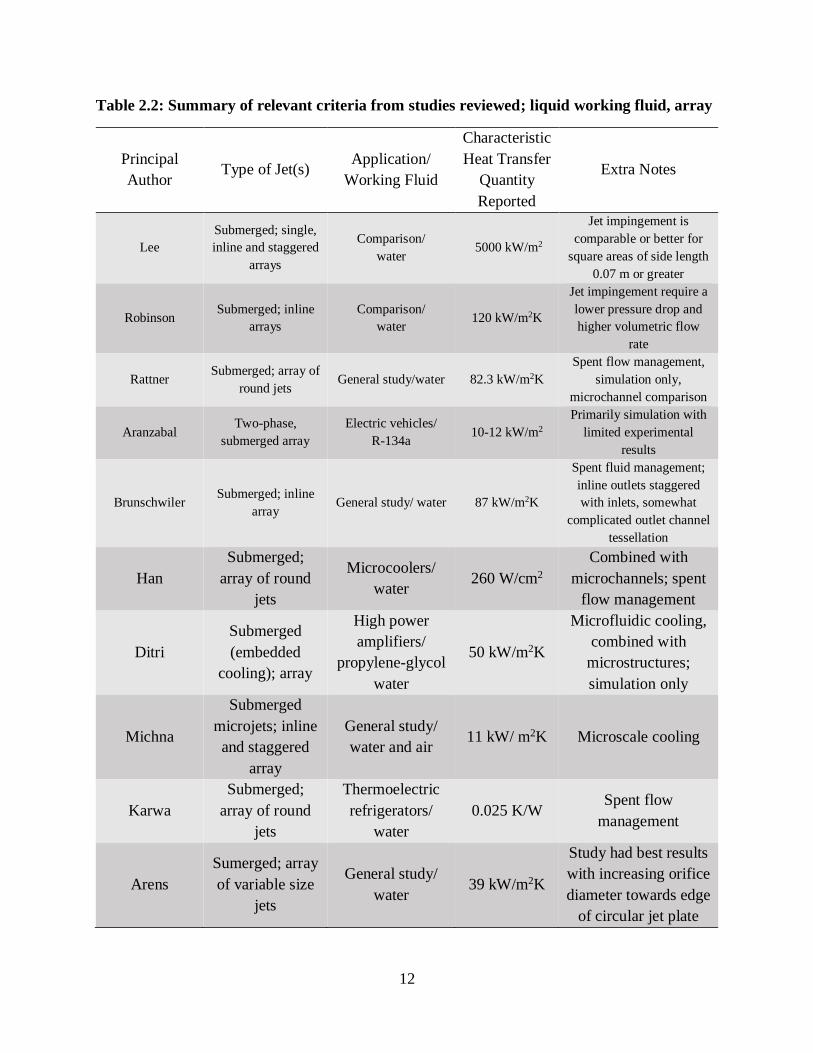
Table 2.2: Summary of relevant criteria from studies reviewed; liquid working fluid, array

Principal

Author Type of Jet(s)

Application/

Working Fluid

Characteristic

Heat Transfer

Quantity

Reported

Extra Notes

Lee

Submerged; single,

inline and staggered

arrays

Comparison/

water 5000 kW/m2

Jet impingement is

comparable or better for

square areas of side length

0.07 m or greater

Robinson Submerged; inline

arrays

Comparison/

water 120 kW/m2K

Jet impingement require a

lower pressure drop and

higher volumetric flow

rate

Rattner Submerged; array of

round jets General study/water 82.3 kW/m2K

Spent flow management,

simulation only,

microchannel comparison

Aranzabal Two-phase,

submerged array

Electric vehicles/

R-134a 10-12 kW/m2

Primarily simulation with

limited experimental

results

Brunschwiler Submerged; inline

array General study/ water 87 kW/m2K

Spent fluid management;

inline outlets staggered

with inlets, somewhat

complicated outlet channel

tessellation

Han

Submerged;

array of round

jets

Microcoolers/

water 260 W/cm2

Combined with

microchannels; spent

flow management

Ditri

Submerged

(embedded

cooling); array

High power

amplifiers/

propylene-glycol

water

50 kW/m2K

Microfluidic cooling,

combined with

microstructures;

simulation only

Michna

Submerged

microjets; inline

and staggered

array

General study/

water and air 11 kW/ m2K Microscale cooling

Karwa

Submerged;

array of round

jets

Thermoelectric

refrigerators/

water

0.025 K/W Spent flow

management

Arens

Sumerged; array

of variable size

jets

General study/

water 39 kW/m2K

Study had best results

with increasing orifice

diameter towards edge

of circular jet plate

13

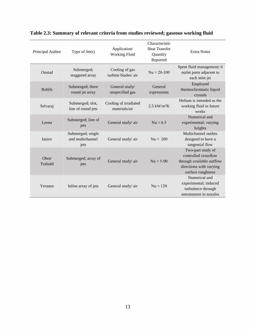
Table 2.3: Summary of relevant criteria from studies reviewed; gaseous working fluid

Principal Author Type of Jet(s) Application/

Working Fluid

Characteristic

Heat Transfer

Quantity

Reported

Extra Notes

Onstad Submerged;

staggered array

Cooling of gas

turbine blades/ air Nu ≈ 20-100

Spent fluid management; 6

outlet ports adjacent to

each inlet jet

Rohlfs Submerged; three

round jet array

General study/

unspecified gas

General

expressions

Employed

thermochromatic liquid

crystals

Selvaraj Submerged; slot,

line of round jets

Cooling of irradiated

materials/air 2.5 kW/m2K

Helium is intended as the

working fluid in future

works

Leena Submerged; line of

jets General study/ air Nu ≈ 6.5

Numerical and

experimental; varying

heights

Ianiro

Submerged; single

and multichannel

jets

General study/ air Nu ≈ 200

Multichannel outlets

designed to have a

tangential flow

Obot/

Trabold

Submerged; array of

jets General study/ air Nu ≈ 5-90

Two-part study of

controlled crossflow

through available outflow

directions with varying

surface roughness

Yeranee Inline array of jets General study/ air Nu ≈ 120

Numerical and

experimental; induced

turbulence through

entrainment in nozzles

14

Chapter 3

Experimental Setup and Procedures

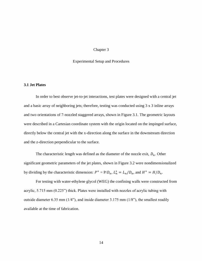
3.1 Jet Plates

In order to best observe jet-to-jet interactions, test plates were designed with a central jet

and a basic array of neighboring jets; therefore, testing was conducted using 3 x 3 inline arrays

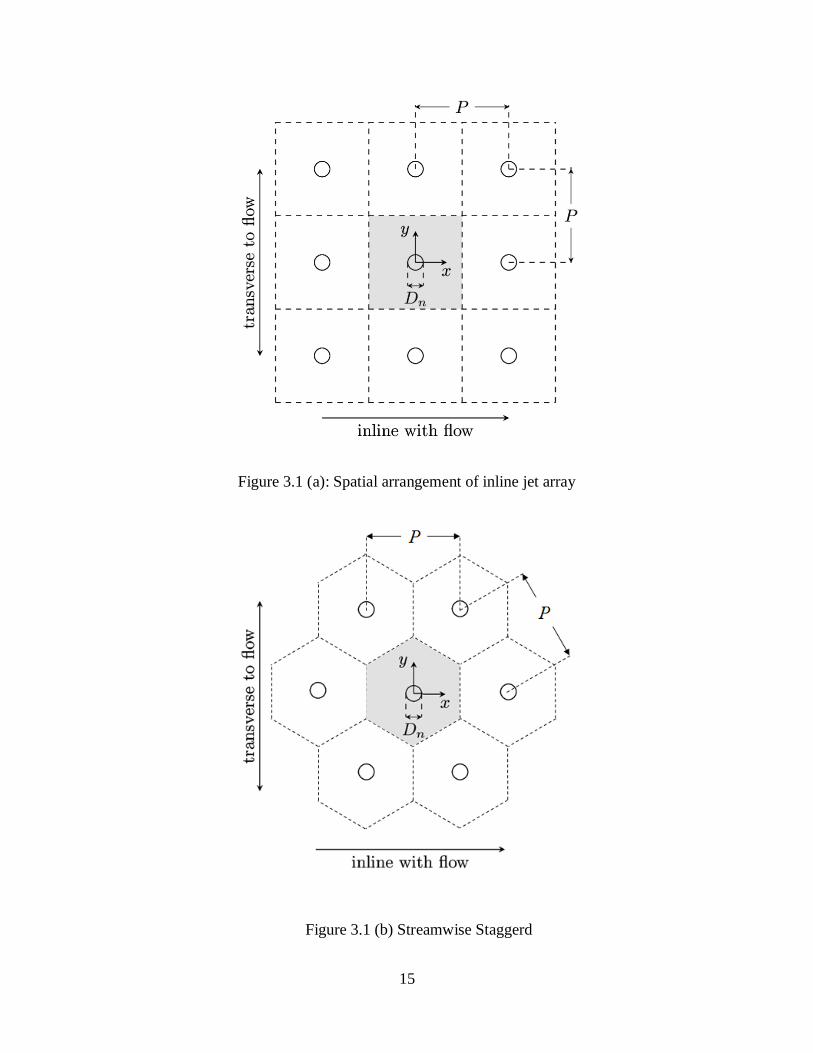
and two orientations of 7-nozzled staggered arrays, shown in Figure 3.1. The geometric layouts

were described in a Cartesian coordinate system with the origin located on the impinged surface,

directly below the central jet with the x-direction along the surface in the downstream direction

and the z-direction perpendicular to the surface.

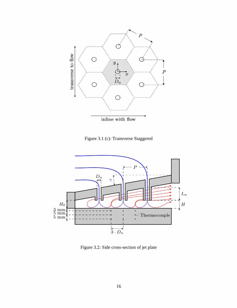
The characteristic length was defined as the diameter of the nozzle exit, 𝐷𝑛. Other

significant geometric parameters of the jet plates, shown in Figure 3.2 were nondimensionalized

by dividing by the characteristic dimension: 𝑃+ = P/𝐷𝑛, 𝐿𝑛+ = 𝐿𝑛/𝐷𝑛, and 𝐻+ = 𝐻/𝐷𝑛.

For testing with water-ethylene glycol (WEG) the confining walls were constructed from

acrylic, 5.715 mm (0.225”) thick. Plates were installed with nozzles of acrylic tubing with

outside diameter 6.35 mm (1/4”), and inside diameter 3.175 mm (1/8”), the smallest readily

available at the time of fabrication.

15

Figure 3.1 (a): Spatial arrangement of inline jet array

Figure 3.1 (b) Streamwise Staggerd

16

Figure 3.1 (c): Transverse Staggered

Figure 3.2: Side cross-section of jet plate

17

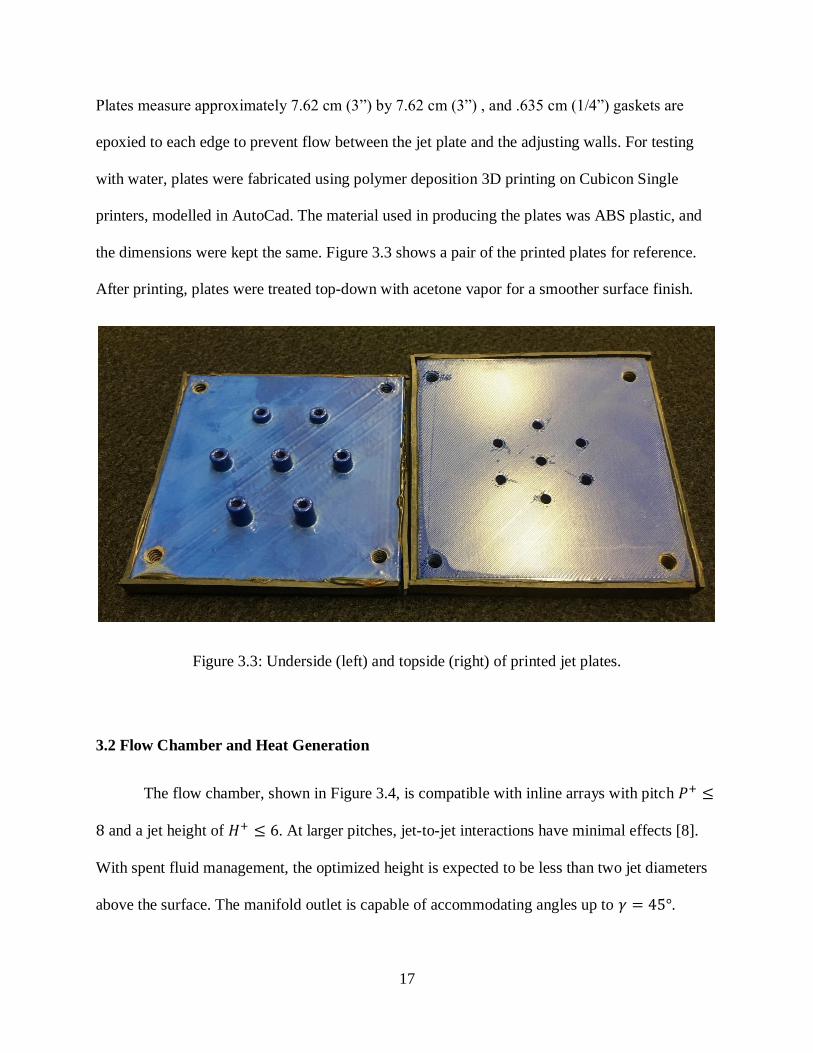
Plates measure approximately 7.62 cm (3”) by 7.62 cm (3”) , and .635 cm (1/4”) gaskets are

epoxied to each edge to prevent flow between the jet plate and the adjusting walls. For testing

with water, plates were fabricated using polymer deposition 3D printing on Cubicon Single

printers, modelled in AutoCad. The material used in producing the plates was ABS plastic, and

the dimensions were kept the same. Figure 3.3 shows a pair of the printed plates for reference.

After printing, plates were treated top-down with acetone vapor for a smoother surface finish.

Figure 3.3: Underside (left) and topside (right) of printed jet plates.

3.2 Flow Chamber and Heat Generation

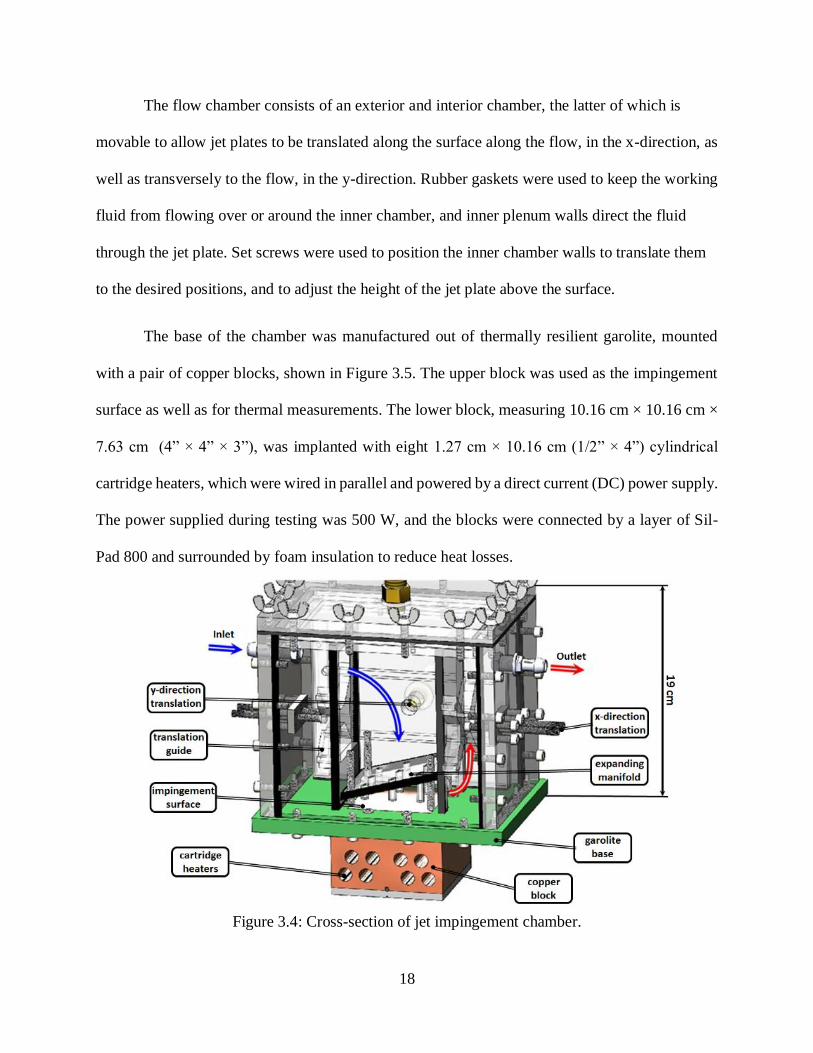
The flow chamber, shown in Figure 3.4, is compatible with inline arrays with pitch 𝑃+ ≤

8 and a jet height of 𝐻+ ≤ 6. At larger pitches, jet-to-jet interactions have minimal effects [8].

With spent fluid management, the optimized height is expected to be less than two jet diameters

above the surface. The manifold outlet is capable of accommodating angles up to 𝛾 = 45°.

18

The flow chamber consists of an exterior and interior chamber, the latter of which is

movable to allow jet plates to be translated along the surface along the flow, in the x-direction, as

well as transversely to the flow, in the y-direction. Rubber gaskets were used to keep the working

fluid from flowing over or around the inner chamber, and inner plenum walls direct the fluid

through the jet plate. Set screws were used to position the inner chamber walls to translate them

to the desired positions, and to adjust the height of the jet plate above the surface.

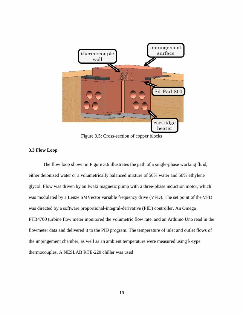
The base of the chamber was manufactured out of thermally resilient garolite, mounted

with a pair of copper blocks, shown in Figure 3.5. The upper block was used as the impingement

surface as well as for thermal measurements. The lower block, measuring 10.16 cm × 10.16 cm ×

7.63 cm (4” × 4” × 3”), was implanted with eight 1.27 cm × 10.16 cm (1/2” × 4”) cylindrical

cartridge heaters, which were wired in parallel and powered by a direct current (DC) power supply.

The power supplied during testing was 500 W, and the blocks were connected by a layer of Sil-

Pad 800 and surrounded by foam insulation to reduce heat losses.

Figure 3.4: Cross-section of jet impingement chamber.

19

Figure 3.5: Cross-section of copper blocks

3.3 Flow Loop

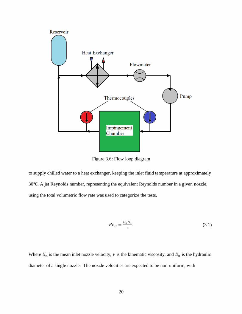
The flow loop shown in Figure 3.6 illustrates the path of a single-phase working fluid,

either deionized water or a volumetrically balanced mixture of 50% water and 50% ethylene

glycol. Flow was driven by an Iwaki magnetic pump with a three-phase induction motor, which

was modulated by a Lenze SMVector variable frequency drive (VFD). The set point of the VFD

was directed by a software proportional-integral-derivative (PID) controller. An Omega

FTB4700 turbine flow meter monitored the volumetric flow rate, and an Arduino Uno read in the

flowmeter data and delivered it to the PID program. The temperature of inlet and outlet flows of

the impingement chamber, as well as an ambient temperature were measured using k-type

thermocouples. A NESLAB RTE-220 chiller was used

20

Figure 3.6: Flow loop diagram

to supply chilled water to a heat exchanger, keeping the inlet fluid temperature at approximately

30℃. A jet Reynolds number, representing the equivalent Reynolds number in a given nozzle,

using the total volumetric flow rate was used to categorize the tests.

𝑅𝑒𝐷 =𝑈𝑛𝐷𝑛

𝜈. (3.1)

Where 𝑈𝑛 is the mean inlet nozzle velocity, 𝜈 is the kinematic viscosity, and 𝐷𝑛 is the hydraulic

diameter of a single nozzle. The nozzle velocities are expected to be non-uniform, with

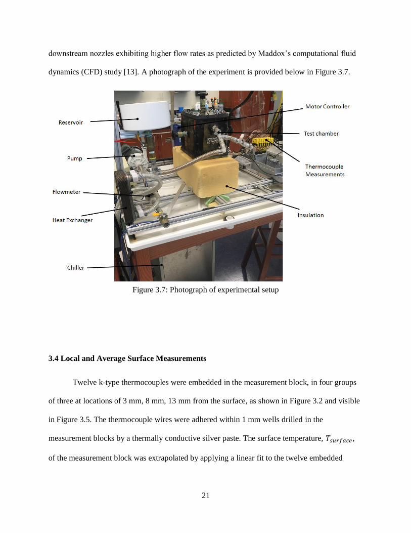
21

downstream nozzles exhibiting higher flow rates as predicted by Maddox’s computational fluid

dynamics (CFD) study [13]. A photograph of the experiment is provided below in Figure 3.7.

3.4 Local and Average Surface Measurements

Twelve k-type thermocouples were embedded in the measurement block, in four groups

of three at locations of 3 mm, 8 mm, 13 mm from the surface, as shown in Figure 3.2 and visible

in Figure 3.5. The thermocouple wires were adhered within 1 mm wells drilled in the

measurement blocks by a thermally conductive silver paste. The surface temperature, 𝑇𝑠𝑢𝑟𝑓𝑎𝑐𝑒 ,

of the measurement block was extrapolated by applying a linear fit to the twelve embedded

Figure 3.7: Photograph of experimental setup

22

thermocouple groups., and combined with the inlet fluid temperature, 𝑇𝑖𝑛𝑙𝑒𝑡 ≈ 30℃, to calculate

the temperature rise at the surface,

Θ = 𝑇𝑠𝑢𝑟𝑓𝑎𝑐𝑒 − 𝑇𝑖𝑛𝑙𝑒𝑡 . (3.2)

The measurement block was used as a heat flux meter by using the gradient measured by

the thermocouples and the known thermal conductivity of copper to determine the local surface

heat fluxes directly above the thermocouple groups,

�̇�′′ = −𝑘𝜕𝑇

𝜕𝑧|𝑧=0. (3.3)

By combining equations (3.2) and (3.3), the local heat transfer coefficient above each

thermocouple group was then estimated,

ℎ =�̇�′′

Θ. (3.4)

These values were in turn used, along with the nozzle diameter and known thermal

properties of water and WEG at a mean fluid temperature, to calculate the local Nusselt number,

𝑁𝑢𝐷ℎ =ℎ𝐷ℎ

𝑘𝑓𝑙𝑢𝑖𝑑. (3.6)

The focus area on the impinged surface for this study is the region around a singular central

jet. In order to fully characterize this region one thermocouple group was located directly

underneath the jet, one group was located three nozzle diameters upstream, one group was located

three nozzle diameters downstream, and only one group located three nozzle diameters in a

transverse direction as reasonable symmetry is assumed about 𝑦 = 0. By translating the jet plate

one diameter at a time across the surface in both the inline, 𝑥∗, and transverse, 𝑦∗, a regular grid

of data points can be formed in relation to the jet positions. A diagram of the data points clustered

23

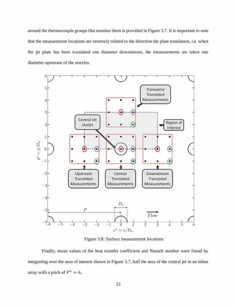
around the thermocouple groups that monitor them is provided in Figure 3.7. It is important to note

that the measurement locations are inversely related to the direction the plate translation, i.e. when

the jet plate has been translated one diameter downstream, the measurements are taken one

diameter upstream of the nozzles.

Finally, mean values of the heat transfer coefficient and Nusselt number were found by

integrating over the area of interest shown in Figure 3.7, half the area of the central jet in an inline

array with a pitch of 𝑃+ = 6,

Figure 3.8: Surface measurement locations

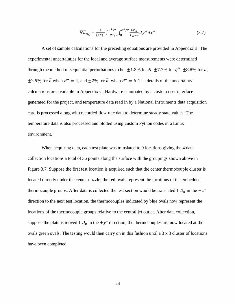
24

𝑁𝑢̅̅ ̅̅ 𝐷𝑛 =2

(𝑃+)2∫ ∫

ℎ𝐷ℎ

𝑘𝑊𝐸𝐺𝑑𝑦+𝑑𝑥+

𝑃+/2

0

𝑃+/2

−𝑃+/2. (3.7)

A set of sample calculations for the preceding equations are provided in Appendix B. The

experimental uncertainties for the local and average surface measurements were determined

through the method of sequential perturbations to be: ±1.2% for 𝛩, ±7.7% for �̇�′′, ±8.8% for ℎ,

±2.5% for ℎ̅ when 𝑃+ = 4, and ±2% for ℎ̅ when 𝑃+ = 6. The details of the uncertainty

calculations are available in Appendix C. Hardware is initiated by a custom user interface

generated for the project, and temperature data read in by a National Instruments data acquisition

card is processed along with recorded flow rate data to determine steady state values. The

temperature data is also processed and plotted using custom Python codes in a Linux

environment.

When acquiring data, each test plate was translated to 9 locations giving the 4 data

collection locations a total of 36 points along the surface with the groupings shown above in

Figure 3.7. Suppose the first test location is acquired such that the center thermocouple cluster is

located directly under the center nozzle; the red ovals represent the locations of the embedded

thermocouple groups. After data is collected the test section would be translated 1 𝐷𝑛 in the −𝑥∗

direction to the next test location, the thermocouples indicated by blue ovals now represent the

locations of the thermocouple groups relative to the central jet outlet. After data collection,

suppose the plate is moved 1 𝐷𝑛 in the +𝑦∗ direction, the thermocouples are now located at the

ovals green ovals. The testing would then carry on in this fashion until a 3 x 3 cluster of locations

have been completed.

25

Chapter 4

Results

4.1 Overview of Parameters Tested

Previous studies with this experimental setup [11-13] focused on proving that using an

expanding manifold had an alleviating effect on entrainment of downstream jets into spent flow

and developing a general correlation for inline arrays with water as the working fluid. The current

experimental study focuses on two major subsequent considerations to be made, and the series of

tests can largely be grouped into two categories.

4.1.1 Water-Ethylene Glycol Tests

Due to the primary target application being the cooling of power electronics in electric vehicles

by employing the existing radiator flow loop, the validity of the expanding area manifold must be

justified with the working fluid of said flow loop, antifreeze or 1:1 volumetric mixture of water-

ethylene glycol, which generally has Prandtl numbers 4-5 times those of water [32]. Tests were

conducted with varying flow rate, manifold angle, and nozzle-to-surface height. Previously

acquired tests with water were used as a reference point. Table 4.1 outlines the geometry

characteristics of the plates used in water-ethylene glycol tests.

26

Table 4.1 Geometric parameters of plates for water-ethylene glycol tests

Pattern Angle,

𝛾

Pitch,

𝑃∗ Height above surface,

𝐻∗ Reynolds Numbers

Inline 0 6 1 5100

Inline 5 6 1 2050, 3000, 4050, 5100

Inline 5 6 2 5100

Inline 10 6 1 5100

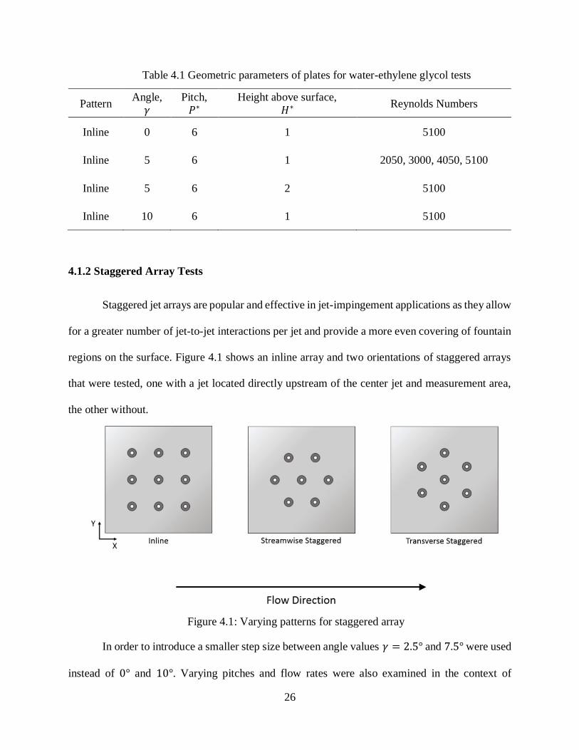
4.1.2 Staggered Array Tests

Staggered jet arrays are popular and effective in jet-impingement applications as they allow

for a greater number of jet-to-jet interactions per jet and provide a more even covering of fountain

regions on the surface. Figure 4.1 shows an inline array and two orientations of staggered arrays

that were tested, one with a jet located directly upstream of the center jet and measurement area,

the other without.

In order to introduce a smaller step size between angle values 𝛾 = 2.5° and 7.5° were used

instead of 0° and 10°. Varying pitches and flow rates were also examined in the context of

Figure 4.1: Varying patterns for staggered array

27

staggered arrays. Table 4.2 outlines the geometric characteristics of the plates used in staggered

array tests. Water was selected as the working fluid for the staggered array tests as it is the simpler

working fluid to employ.

Table 4.2 Geometric parameters of plates for staggered tests

Pattern Angle,

𝛾

Pitch,

𝑃∗ Reynolds Numbers

Streamwise staggered 5 3 8400, 11200, 14000

Streamwise staggered 2.5 4 5600, 8400, 11200, 14000

Streamwise staggered 5 4 5600, 8400, 11200, 14000

Streamwise staggered 7.5 4 5600, 8400, 11200, 14000

Streamwise staggered 2.5 6 5600, 8400, 11200, 14000

Streamwise staggered 5 6 5600, 8400, 11200, 14000

Streamwise staggered 7.5 6 5600, 8400, 11200, 14000

Transverse staggered 2.5 6 5600, 8400, 11200, 14000

Transverse staggered 5 6 5600, 8400, 11200, 14000

Transverse staggered 7.5 6 5600, 8400, 11200, 14000

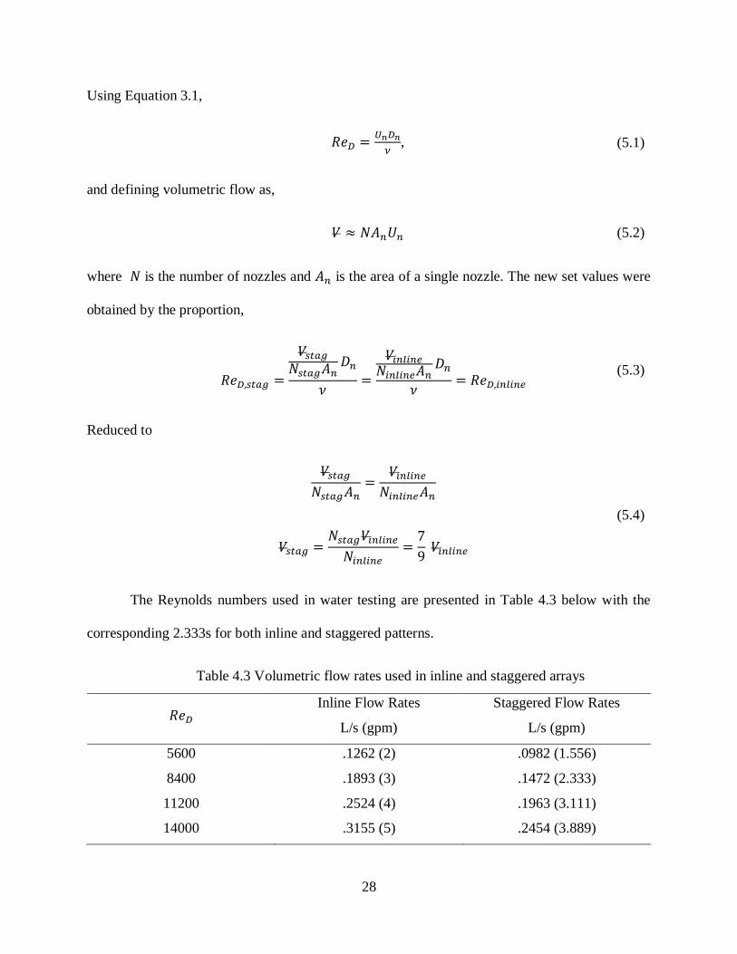
In order to be more comparable to earlier work with water [11-13], it was decided that tests

should be conducted at the same Reynolds numbers as before. Additionally, nozzle diameter was

held constant, meaning the average nozzle velocity, or rather Arduino controlled volumetric flow

rates, 𝑉, would need to be adjusted.

28

Using Equation 3.1,

𝑅𝑒𝐷 =𝑈𝑛𝐷𝑛

𝜈, (5.1)

and defining volumetric flow as,

𝑉 ≈ 𝑁𝐴𝑛𝑈𝑛 (5.2)

where 𝑁 is the number of nozzles and 𝐴𝑛 is the area of a single nozzle. The new set values were

obtained by the proportion,

𝑅𝑒𝐷,𝑠𝑡𝑎𝑔 =

𝑉𝑠𝑡𝑎𝑔𝑁𝑠𝑡𝑎𝑔𝐴𝑛

𝐷𝑛

𝜈=

𝑉𝑖𝑛𝑙𝑖𝑛𝑒𝑁𝑖𝑛𝑙𝑖𝑛𝑒𝐴𝑛

𝐷𝑛

𝜈= 𝑅𝑒𝐷,𝑖𝑛𝑙𝑖𝑛𝑒

(5.3)

Reduced to

𝑉𝑠𝑡𝑎𝑔𝑁𝑠𝑡𝑎𝑔𝐴𝑛

=𝑉𝑖𝑛𝑙𝑖𝑛𝑒𝑁𝑖𝑛𝑙𝑖𝑛𝑒𝐴𝑛

𝑉𝑠𝑡𝑎𝑔 =𝑁𝑠𝑡𝑎𝑔𝑉𝑖𝑛𝑙𝑖𝑛𝑒𝑁𝑖𝑛𝑙𝑖𝑛𝑒

=7

9 𝑉𝑖𝑛𝑙𝑖𝑛𝑒

(5.4)

The Reynolds numbers used in water testing are presented in Table 4.3 below with the

corresponding 2.333s for both inline and staggered patterns.

Table 4.3 Volumetric flow rates used in inline and staggered arrays

𝑅𝑒𝐷 Inline Flow Rates

L/s (gpm)

Staggered Flow Rates

L/s (gpm)

5600 .1262 (2) .0982 (1.556)

8400 .1893 (3) .1472 (2.333)

11200 .2524 (4) .1963 (3.111)

14000 .3155 (5) .2454 (3.889)

29

4.2 Water-Ethylene Glycol Results and Discussion

A complete set of results is provided in Appendix D. The most significant results are

presented in the following paragraphs to highlight the effects of varying Reynolds number,

manifold angle, and jet-to-surface spacing with water-ethylene glycol flowing through inline

arrays.

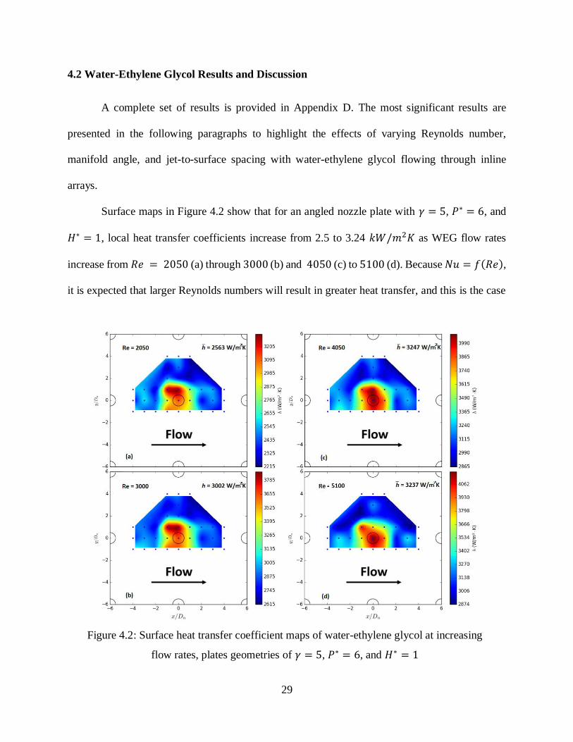
Surface maps in Figure 4.2 show that for an angled nozzle plate with 𝛾 = 5, 𝑃∗ = 6, and

𝐻∗ = 1, local heat transfer coefficients increase from 2.5 to 3.24 𝑘𝑊/𝑚2𝐾 as WEG flow rates

increase from 𝑅𝑒 = 2050 (a) through 3000 (b) and 4050 (c) to 5100 (d). Because 𝑁𝑢 = 𝑓(𝑅𝑒),

it is expected that larger Reynolds numbers will result in greater heat transfer, and this is the case

Figure 4.2: Surface heat transfer coefficient maps of water-ethylene glycol at increasing

flow rates, plates geometries of 𝛾 = 5, 𝑃∗ = 6, and 𝐻∗ = 1

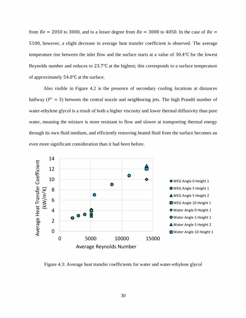
30

from 𝑅𝑒 = 2050 to 3000, and to a lesser degree from 𝑅𝑒 = 3000 to 4050. In the case of 𝑅𝑒 =

5100, however, a slight decrease in average heat transfer coefficient is observed. The average

temperature rise between the inlet flow and the surface starts at a value of 30.4℃ for the lowest

Reynolds number and reduces to 23.7℃ at the highest; this corresponds to a surface temperature

of approximately 54.0℃ at the surface.

Also visible in Figure 4.2 is the presence of secondary cooling locations at distances

halfway (𝑃∗ = 3) between the central nozzle and neighboring jets. The high Prandtl number of

water-ethylene glycol is a result of both a higher viscosity and lower thermal diffusivity than pure

water, meaning the mixture is more resistant to flow and slower at transporting thermal energy

through its own fluid medium, and efficiently removing heated fluid from the surface becomes an

even more significant consideration than it had been before.

Figure 4.3: Average heat transfer coefficients for water and water-ethylene glycol

0

2

4

6

8

10

12

14

0 5000 10000 15000

Ave

rage

He

at T

ran

sfe

r C

oe

ffic

ien

t (k

W/m

2K

)

Average Reynolds Number

WEG Angle 0 Height 1

WEG Angle 5 Height 1

WEG Angle 5 Height 2

WEG Angle 10 Height 1

Water Angle 0 Height 1

Water Angle 5 Height 1

Water Angle 5 Height 2

Water Angle 10 Height 1

31

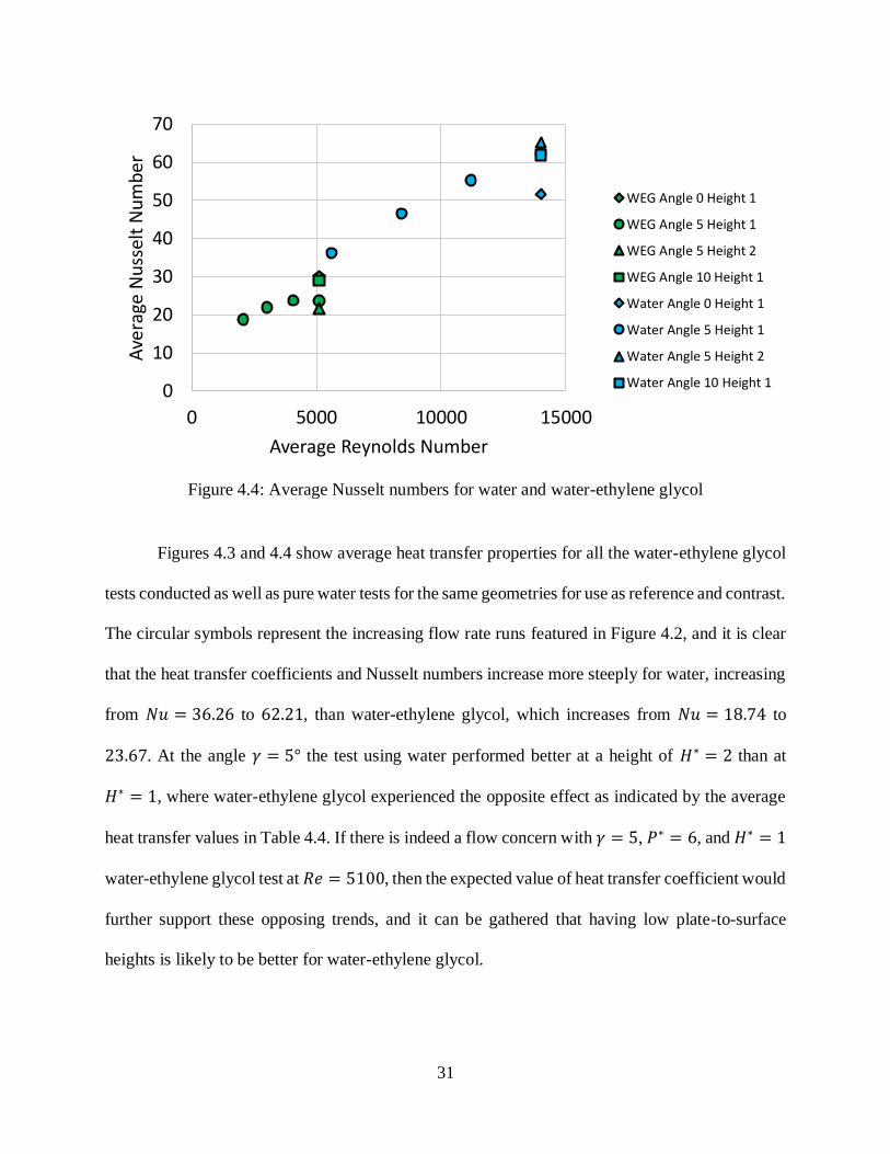
Figure 4.4: Average Nusselt numbers for water and water-ethylene glycol

Figures 4.3 and 4.4 show average heat transfer properties for all the water-ethylene glycol

tests conducted as well as pure water tests for the same geometries for use as reference and contrast.

The circular symbols represent the increasing flow rate runs featured in Figure 4.2, and it is clear

that the heat transfer coefficients and Nusselt numbers increase more steeply for water, increasing

from 𝑁𝑢 = 36.26 to 62.21, than water-ethylene glycol, which increases from 𝑁𝑢 = 18.74 to

23.67. At the angle 𝛾 = 5° the test using water performed better at a height of 𝐻∗ = 2 than at

𝐻∗ = 1, where water-ethylene glycol experienced the opposite effect as indicated by the average

heat transfer values in Table 4.4. If there is indeed a flow concern with 𝛾 = 5, 𝑃∗ = 6, and 𝐻∗ = 1

water-ethylene glycol test at 𝑅𝑒 = 5100, then the expected value of heat transfer coefficient would

further support these opposing trends, and it can be gathered that having low plate-to-surface

heights is likely to be better for water-ethylene glycol.

0

10

20

30

40

50

60

70

0 5000 10000 15000

Ave

rage

Nu

ssel

t N

um

ber

Average Reynolds Number

WEG Angle 0 Height 1

WEG Angle 5 Height 1

WEG Angle 5 Height 2

WEG Angle 10 Height 1

Water Angle 0 Height 1

Water Angle 5 Height 1

Water Angle 5 Height 2

Water Angle 10 Height 1

32

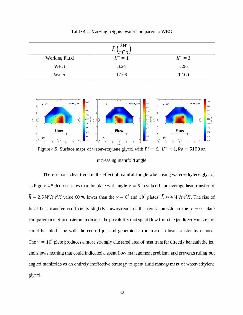
Table 4.4: Varying heights: water compared to WEG

ℎ̅ (𝑘𝑊

𝑚2𝐾)

Working Fluid 𝐻∗ = 1 𝐻∗ = 2

WEG 3.24 2.96

Water 12.08 12.66

Figure 4.5: Surface maps of water-ethylene glycol with 𝑃∗ = 6, 𝐻∗ = 1,𝑅𝑒 = 5100 an

increasing manifold angle

There is not a clear trend in the effect of manifold angle when using water-ethylene glycol,

as Figure 4.5 demonstrates that the plate with angle 𝛾 = 5° resulted in an average heat transfer of

ℎ̅ = 2.5 𝑊/𝑚2𝐾 value 60 % lower than the 𝛾 = 0° and 10° plates’ ℎ̅ ≈ 4 𝑊/𝑚2𝐾. The rise of

local heat transfer coefficients slightly downstream of the central nozzle in the 𝛾 = 0° plate

compared to region upstream indicates the possibility that spent flow from the jet directly upstream

could be interfering with the central jet, and generated an increase in heat transfer by chance.

The 𝛾 = 10° plate produces a more strongly clustered area of heat transfer directly beneath the jet,

and shows nothing that could indicated a spent flow management problem, and prevents ruling out

angled manifolds as an entirely ineffective strategy to spent fluid management of water-ethylene

glycol.

33

The study by Narumanchi [5] is significantly different in terms of geometry, i.e. number

of nozzles used, surface features applied, and diameter of nozzle, and has results that focus on

qualities ranging from surface wear to coefficient of performance to heat transfer coefficient;

despite this there is one available line of comparison in what Narumanchi’s group refers to as

temperature uniformity, or the difference between the maximum and minimum temperatures for a

given test. Narumanchi reported 2.7℃ for their plain, circular surface with diameter 1.4 𝑚𝑚,

where the results of the current study observed temperature uniformities ranging from 1.0℃ to

3.5℃ over a larger square area with side length 76.2 𝑚𝑚. The smaller ranges seen over the larger

area in the current study support the case for water-ethylene glycol’s compatibility with jet

impingement arrays and angled confining walls.

4.3 Staggered Array Results and Discussion

A complete set of results is presented in Appendix D. The most significant results are

presented in the following paragraphs to highlight the effects of varying nozzle patterns,

manifold angle, and pitch in conjunction with water flowing through staggered arrays.

Figure 4.6 shows extrapolated surface maps of temperature rise for the various array

patterns tested. The lowest temperature rises are seen for the in-line array (a) with values ranging

between around 6 and 6.6 degrees. The highest temperature rises of 11.5 to 13 degrees are on the

transverse staggered array (c), where there is no jet directly upstream from the center jet. This

highlights the unevenness of cooling that could be expected along in the upstream portion of an

expanded staggered array. The streamwise staggered array with the 𝑃∗ = 6 (b) was able to keep

the temperature rise below 10 degrees, but the array with a 𝑃∗ = 4 (d) has the most pronounced

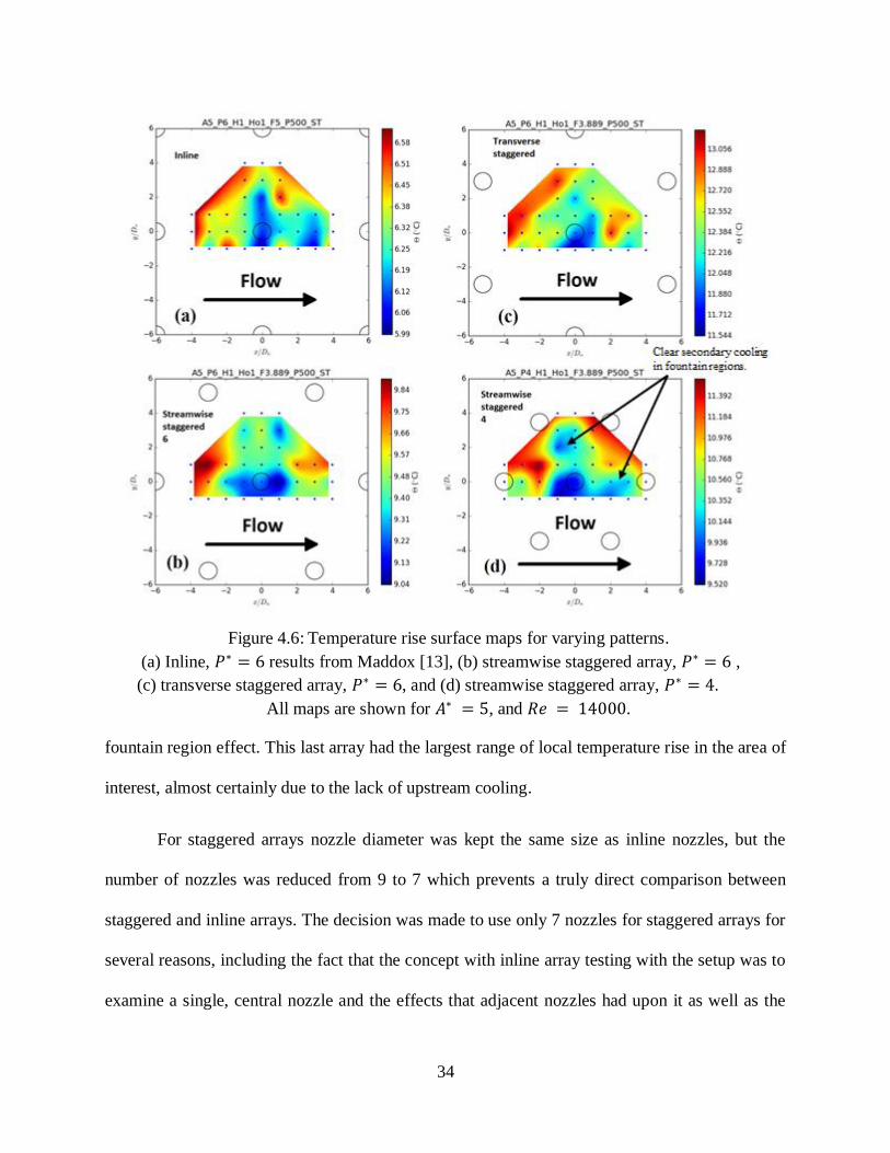
34

fountain region effect. This last array had the largest range of local temperature rise in the area of

interest, almost certainly due to the lack of upstream cooling.

For staggered arrays nozzle diameter was kept the same size as inline nozzles, but the

number of nozzles was reduced from 9 to 7 which prevents a truly direct comparison between

staggered and inline arrays. The decision was made to use only 7 nozzles for staggered arrays for

several reasons, including the fact that the concept with inline array testing with the setup was to

examine a single, central nozzle and the effects that adjacent nozzles had upon it as well as the

Figure 4.6: Temperature rise surface maps for varying patterns.

(a) Inline, 𝑃∗ = 6 results from Maddox [13], (b) streamwise staggered array, 𝑃∗ = 6 ,

(c) transverse staggered array, 𝑃∗ = 6, and (d) streamwise staggered array, 𝑃∗ = 4.

All maps are shown for 𝐴∗ = 5, and 𝑅𝑒 = 14000.

35

limitations of where nozzles could be placed and still be entirely on the plate and the concern of

wall effects.

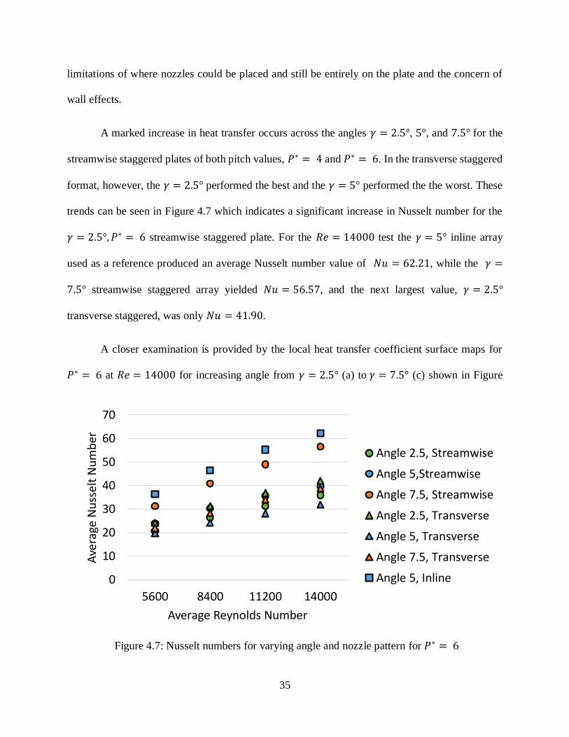
A marked increase in heat transfer occurs across the angles 𝛾 = 2.5°, 5°, and 7.5° for the

streamwise staggered plates of both pitch values, 𝑃∗ = 4 and 𝑃∗ = 6. In the transverse staggered

format, however, the 𝛾 = 2.5° performed the best and the 𝛾 = 5° performed the the worst. These

trends can be seen in Figure 4.7 which indicates a significant increase in Nusselt number for the

𝛾 = 2.5°, 𝑃∗ = 6 streamwise staggered plate. For the 𝑅𝑒 = 14000 test the 𝛾 = 5° inline array

used as a reference produced an average Nusselt number value of 𝑁𝑢 = 62.21, while the 𝛾 =

7.5° streamwise staggered array yielded 𝑁𝑢 = 56.57, and the next largest value, 𝛾 = 2.5°

transverse staggered, was only 𝑁𝑢 = 41.90.

A closer examination is provided by the local heat transfer coefficient surface maps for

𝑃∗ = 6 at 𝑅𝑒 = 14000 for increasing angle from 𝛾 = 2.5° (a) to 𝛾 = 7.5° (c) shown in Figure

0

10

20

30

40

50

60

70

5600 8400 11200 14000

Ave

rage

Nu

ssel

t N

um

ber

Average Reynolds Number

Angle 2.5, Streamwise

Angle 5,Streamwise

Angle 7.5, Streamwise

Angle 2.5, Transverse

Angle 5, Transverse

Angle 7.5, Transverse

Angle 5, Inline

Figure 4.7: Nusselt numbers for varying angle and nozzle pattern for 𝑃∗ = 6

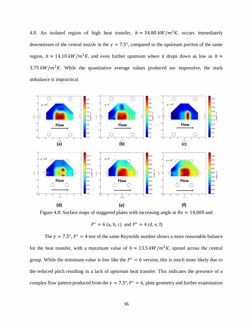
36

4.8. An isolated region of high heat transfer, ℎ ≈ 34.80 𝑘𝑊/𝑚2𝐾, occurs immediately

downstream of the central nozzle in the 𝛾 = 7.5°, compared to the upstream portion of the same

region, ℎ ≈ 14.10 𝑘𝑊/𝑚2𝐾, and even further upstream where it drops down as low as ℎ ≈

3.75 𝑘𝑊/𝑚2𝐾. While the quantitative average values produced are impressive, the stark

imbalance is impractical.

Figure 4.8: Surface maps of staggered plates with increasing angle at 𝑅𝑒 = 14,000 and

𝑃∗ = 6 (a, b, c) and 𝑃∗ = 4 (d, e, f)

The 𝛾 = 7.5°, 𝑃∗ = 4 test of the same Reynolds number shows a more reasonable balance

for the heat transfer, with a maximum value of ℎ ≈ 13.5 𝑘𝑊/𝑚2𝐾, spread across the central

group. While the minimum value is low like the 𝑃∗ = 6 version, this is much more likely due to

the reduced pitch resulting in a lack of upstream heat transfer. This indicates the presence of a

complex flow pattern produced from the 𝛾 = 7.5°, 𝑃∗ = 6, plate geometry and further examination

37

should be carried out with this and similar geometries for greater understanding. Additional flow

rates are presented in Appendix D.

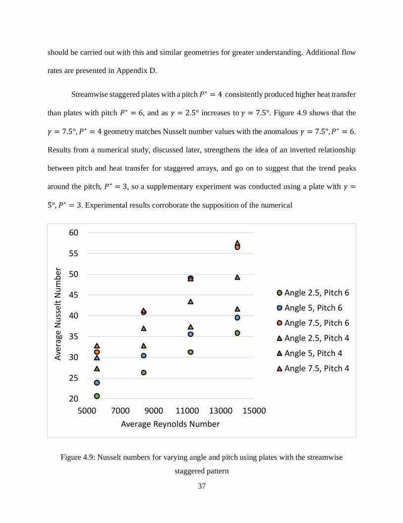
Streamwise staggered plates with a pitch 𝑃∗ = 4 consistently produced higher heat transfer

than plates with pitch 𝑃∗ = 6, and as 𝛾 = 2.5° increases to 𝛾 = 7.5°. Figure 4.9 shows that the

𝛾 = 7.5°, 𝑃∗ = 4 geometry matches Nusselt number values with the anomalous 𝛾 = 7.5°, 𝑃∗ = 6.

Results from a numerical study, discussed later, strengthens the idea of an inverted relationship

between pitch and heat transfer for staggered arrays, and go on to suggest that the trend peaks

around the pitch, 𝑃∗ = 3, so a supplementary experiment was conducted using a plate with 𝛾 =

5°, 𝑃∗ = 3. Experimental results corroborate the supposition of the numerical

Figure 4.9: Nusselt numbers for varying angle and pitch using plates with the streamwise

staggered pattern

20

25

30

35

40

45

50

55

60

5000 7000 9000 11000 13000 15000

Ave

rage

Nu

ssel

t N

um

ber

Average Reynolds Number

Angle 2.5, Pitch 6

Angle 5, Pitch 6

Angle 7.5, Pitch 6

Angle 2.5, Pitch 4

Angle 5, Pitch 4

Angle 7.5, Pitch 4

38

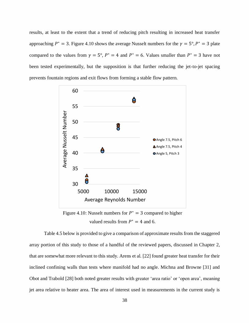
results, at least to the extent that a trend of reducing pitch resulting in increased heat transfer

approaching 𝑃∗ = 3. Figure 4.10 shows the average Nusselt numbers for the 𝛾 = 5°, 𝑃∗ = 3 plate

compared to the values from 𝛾 = 5°, 𝑃∗ = 4 and 𝑃∗ = 6. Values smaller than 𝑃∗ = 3 have not

been tested experimentally, but the supposition is that further reducing the jet-to-jet spacing

prevents fountain regions and exit flows from forming a stable flow pattern.

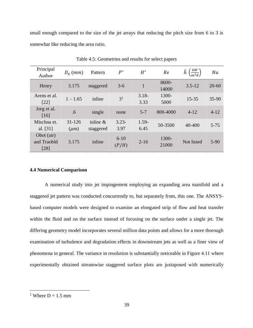
Table 4.5 below is provided to give a comparison of approximate results from the staggered

array portion of this study to those of a handful of the reviewed papers, discussed in Chapter 2,

that are somewhat more relevant to this study. Arens et al. [22] found greater heat transfer for their

inclined confining walls than tests where manifold had no angle. Michna and Browne [31] and

Obot and Trabold [28] both noted greater results with greater ‘area ratio’ or ‘open area’, meaning

jet area relative to heater area. The area of interest used in measurements in the current study is

30

35

40

45

50

55

60

5000 10000 15000

Ave

rage

Nu

ssel

t N

um

ber

Average Reynolds Number

Angle 7.5, Pitch 6

Angle 7.5, Pitch 4

Angle 5, Pitch 3

Figure 4.10: Nusselt numbers for 𝑃∗ = 3 compared to higher

valued results from 𝑃∗ = 4 and 6.

39

small enough compared to the size of the jet arrays that reducing the pitch size from 6 to 3 is

somewhat like reducing the area ratio.

Table 4.5: Geometries and results for select papers

Principal

Author 𝐷𝑛 (𝑚𝑚) Pattern 𝑃∗ 𝐻∗ 𝑅𝑒 ℎ̅ (

𝑘𝑊

𝑚2𝐾) 𝑁𝑢

Henry 3.175 staggered 3-6 1 8600-

14000 3.5-12 20-60

Arens et al.

[22] 1 – 1.65 inline 31

3.18-

3.33

1300-

5000 15-35 35-90

Jorg et al.

[16] .6 single none 5-7 800-4000 4-12 4-12

Mischna et.

al. [31]

31-126

(𝜇m)

inline &

staggered

3.23-

3.97

1.59-

6.45 50-3500 40-400 5-75

Obot (air)

and Traobld

[28]

3.175 inline 6-10

(𝑃/𝐻) 2-16

1300-

21000 Not listed 5-90

4.4 Numerical Comparison

A numerical study into jet impingement employing an expanding area manifold and a

staggered jet pattern was conducted concurrently to, but separately from, this one. The ANSYS-

based computer models were designed to examine an elongated strip of flow and heat transfer

within the fluid and on the surface instead of focusing on the surface under a single jet. The

differing geometry model incorporates several million data points and allows for a more thorough

examination of turbulence and degradation effects in downstream jets as well as a finer view of

phenomena in general. The variance in resolution is substantially noticeable in Figure 4.11 where

experimentally obtained streamwise staggered surface plots are juxtaposed with numerically

1 Where D = 1.5 mm

40

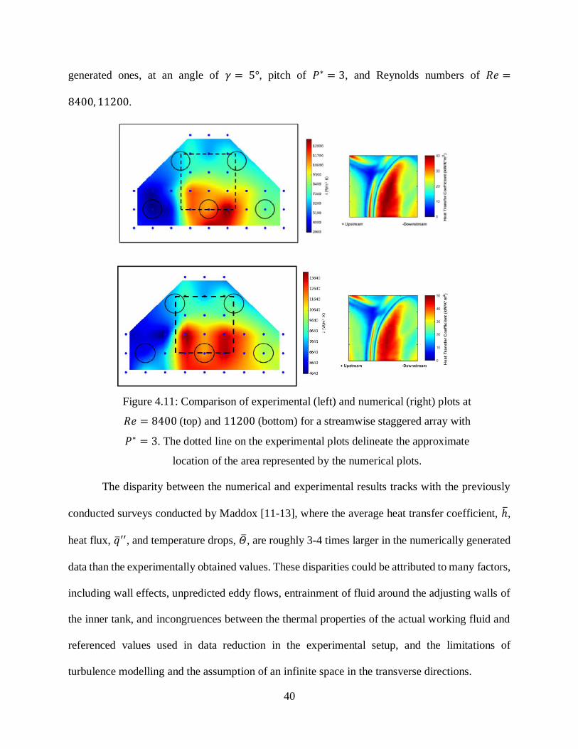
generated ones, at an angle of 𝛾 = 5°, pitch of 𝑃∗ = 3, and Reynolds numbers of 𝑅𝑒 =

8400, 11200.

The disparity between the numerical and experimental results tracks with the previously

conducted surveys conducted by Maddox [11-13], where the average heat transfer coefficient, ℎ̅,

heat flux, �̅�′′, and temperature drops, �̅�, are roughly 3-4 times larger in the numerically generated

data than the experimentally obtained values. These disparities could be attributed to many factors,

including wall effects, unpredicted eddy flows, entrainment of fluid around the adjusting walls of

the inner tank, and incongruences between the thermal properties of the actual working fluid and

referenced values used in data reduction in the experimental setup, and the limitations of

turbulence modelling and the assumption of an infinite space in the transverse directions.

Figure 4.11: Comparison of experimental (left) and numerical (right) plots at

𝑅𝑒 = 8400 (top) and 11200 (bottom) for a streamwise staggered array with

𝑃∗ = 3. The dotted line on the experimental plots delineate the approximate

location of the area represented by the numerical plots.

41

In both experimentally and numerically obtained results, trends were observed to suggest

that heat transfer increases with increasing Reynolds numbers, ℎ,̅ 𝑁𝑢̅̅ ̅̅ ∝ 𝑅𝑒, between 𝑅𝑒 = 5600

and 14000, increasing manifold angle, ℎ,̅ 𝑁𝑢̅̅ ̅̅ ∝ 𝛾, between 𝛾 = 0° and 15°, and decreasing pitch,

ℎ,̅ 𝑁𝑢̅̅ ̅̅ ∝1

𝑃∗, between 𝑃∗ = 3 and 𝑃∗ = 6. At pitches smaller than 𝑃∗ = 3, the numerical study

found that the proximity of jets suppressed the formation of steady fountain flow patterns. The

numerical study also found that the entrainment of jet flows into spent fluid is reduced when angled

confining walls are employed.

42

Chapter 5

Conclusions

Liquid jet impingement can operate with relatively high volumetric flow rates and low

pressure drops, making impinging jets more tenable as a cooling system than other popular liquid

cooling techniques. In larger scale applications, the greatest problem in jet impingement cooling

is the entrainment of downstream jets into the crossflow of spent fluid. A scheme of employing an

expanding area manifold to allow spent fluid a recourse was used for alleviating this effect.

An experimental setup was utilized to characterize changes in the heat transfer with varying

geometries, flow rates, and working fluids. The setup was designed to be capable of recording

local temperature, local surface heat transfer coefficient, and local surface heat flux data. A finer

set of data was obtained by translating the test section across the surface to known points relative

to measurement locations. The larger data set was then used to generate 2-D maps of the local

thermal properties.

The applicability of water-ethylene glycol as a working fluid in this spent-fluid management

scheme was examined using the parameters of Reynolds number, jet-to-surface height, and

manifold angle containing a 3 x 3 inline array of submerged, normal, single-phase, liquid jets. The

highest value of heat transfer coefficient observed with water-ethylene glycol testing was

4,000 𝑊/𝑚2𝐾 when 𝛾 = 0° and 5°, but for 𝛾 = 0° , distorted heat transfer coefficient values

point towards jet degradation. The angled confining wall had mixed results, and when considering

43

the thermophysical properties of water-ethylene glycol, greater impacts may be seen when

employing smaller pitch arrays.

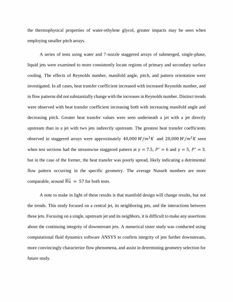
A series of tests using water and 7-nozzle staggered arrays of submerged, single-phase,

liquid jets were examined to more consistently locate regions of primary and secondary surface

cooling. The effects of Reynolds number, manifold angle, pitch, and pattern orientation were

investigated. In all cases, heat transfer coefficient increased with increased Reynolds number, and

in flow patterns did not substantially change with the increases in Reynolds number. Distinct trends

were observed with heat transfer coefficient increasing both with increasing manifold angle and

decreasing pitch. Greater heat transfer values were seen underneath a jet with a jet directly

upstream than in a jet with two jets indirectly upstream. The greatest heat transfer coefficients

observed in staggered arrays were approximately 40,000 𝑊/𝑚2𝐾 and 20,000 𝑊/𝑚2𝐾 seen

when test sections had the streamwise staggered pattern at 𝛾 = 7.5, 𝑃∗ = 6 and 𝛾 = 5, 𝑃∗ = 3.

but in the case of the former, the heat transfer was poorly spread, likely indicating a detrimental

flow pattern occurring in the specific geometry. The average Nusselt numbers are more

comparable, around 𝑁𝑢̅̅ ̅̅ = 57 for both tests.

A note to make in light of these results is that manifold design will change results, but not

the trends. This study focused on a central jet, its neighboring jets, and the interactions between

these jets. Focusing on a single, upstream jet and its neighbors, it is difficult to make any assertions

about the continuing integrity of downstream jets. A numerical sister study was conducted using

computational fluid dynamics software ANSYS to confirm integrity of jets further downstream,

more convincingly characterize flow phenomena, and assist in determining geometry selection for

future study.

44

5.1 Suggestions for future work

As an empirical field of study, jet impingement requires a lot of experimental information

to be accrued to make solid conclusions, and the accuracy of the conclusions can generally be

improved by expanding the amount of data amassed. This means that further testing of topics in

this study would be valuable:

• Inline arrays using water-ethylene glycol

• Investigating an expansion on the range of angles, heights, pitches, and other values for

staggered array with water beyond the results presented in this paper.

• Staggered arrays using water-ethylene glycol

• Downstream testing with angled manifolds1

• Flow and heat transfer characteristics edge of staggered arrays1

Simple jet impingement has a large numer of parameters that can serve as the focus of

study. Adding in any substantial change, such as a spent fluid management strategy, for a specific

application or otherwise, warrants that all the considerations for simple jet impingement be re-

examined, including any other substantial changes that may be compatible. For example, a spent

fluid strategy can often be combined with a modification to inlet flow as shown by Ianiro and

Cardone, Arens, et. al., and Trabold and Odot [21, 22, 27], or an enhancement to the surface as

Moreno, et. al., Narumanchi, et. al., and several other groups have done [1, 5, 18, 24 -26, 29]. One

could go even beyond that and mix a large number of changes, i.e. the modifications presented by

each of Ianiro and Cardone, Arens, et. al., and Trabold and Odot do not prevent any of the others

from also being applied. Therefore individual suggestions listed below are parameters that can be

1 Would likely require a substantial change to setup

45

tested in conjunction with staggered arrays and an expanding manifold spent, but do not preclude

other suggestions from also being investigated. Reviewed papers from Chapter 2 that deal with the

suggested topics are referenced.

• Inlet/outlet geometry of jets to ease pressure drop [4]

• Outlet geometry to induce turbulence in jet

• Surface roughness within nozzle [27]

• An array of jets with increased diameter at the edge of the array [22] or similar

change to compensate for weak heat transfer at boundaries

• Angled jets instead of normal ones

• Internal geometry that generates to induce tangential flow [21]

• Microstructures/roughness on the heated surface1 [1, 5, 18, 24 -26, 29]

• Orientation of the heated surface1

1Would require a substantial change to setup

46

Bibliography

[1] Moreno, Gilbert. "Power electronics thermal management R&D." Retrieved September, 15 2016

from http://www.nrel.gov/docs/fy16osti/64943.pdf, (2016).

[2] Lee, D.-Y., and Vafai, K. “Comparative analysis of jet impingement and microchannel cooling for

high heat flux applications”. Int. J. Mass Heat Trans., 42(9), pp. 1555–1568, (1999).

[3] Robinson, A. J. “A thermal–hydraulic comparison of liquid microchannel and impinging liquid jet

array heat sinks for high-power electronics cooling”. Components and Packaging Technologies,

IEEE Transactions on, 32(2), pp. 347–357, (2009).

[4] Whelan, B. P., and Robinson, A. J., “Nozzle geometry effects in liquid jet array impingement”.

Applied Thermal Engineering, 29(11), pp. 2211–2221, 2009.

[5] Narumanchi, S., Mihalic, M., Moreno, G., and Bennion, K. “Design of light-weight, single-phase

liquidcooled heat exchanger for power electronics”. In the 13th Intersociety Conference on

Thermal and Thermomechanical Phenomena in Electric Systems (ITHERM), 2012, IEEE, pp.

693–699.

[6] Rattner, A. S. “General characterization of jet impingement array heat sinks with interspersed fluid

extraction ports for uniform high-flux cooling”. ASME. J. Heat Transfer. 2017.

[7] Aranzabal, I., Martinez de Alegria, J. I., Garate, J., Andreu and Delmonte, N. "Two-phase liquid

cooling for electric vehicle IGBT power module thermal management," 2017 11th IEEE

International Conference on Compatibility, Power Electronics and Power Engineering (CPE-

POWERENG), Cadiz, 2017, pp. 495-500.

[8] Zuckerman, N. and Lior, N. “Jet impingement heat transfer: Physics, correlations, and numerical

modeling,” Adv. in Heat Trans., 39(06):565-631. (2006).

47

[9] Brunschwiler, T., Rothuizen, H., Fabbri, M., Kloter, U., Michel, B., Bezama, R., and Natarajan, G.,

2006. “Direct liquid jet-impingment cooling with micron-sized nozzle array and distributed

return architecture”. In the 10th Intersociety Conference on Thermal and Thermomechanical

Phenomena in Electronics Systems (ITHERM), 2006, IEEE, pp. 196–203.

[10] Onstad, A. J., Elkins, C. J., Moffat, R. J., and Eaton, J. K., 2009. “Full-field flow measurements and

heat transfer of a compact jet impingement array with local extraction of spent fluid”. Journal of

Heat Transfer, 131(8), p. 082201.

[11] Maddox, J.F., Knight, R.W., Bhavnani, S.H. and Pool, J. "Correlation for single phase liquid jet

impingement with an angled confining wall for power electronics cooling." Proc 15th Int. Conf.

on Therm. and Thermomech. Phen. in Elect. Sys. (ITHERM), IEEE, (2016).

[12] Maddox, J.F., Knight, R.W. and Bhavnani, S.H. “Local thermal measurements of a confined array

of impinging liquid jets for power electronics cooling”. Therm. Meas., Modeling & Management

Symp. (SEMI-THERM), 2015 31st , pp. 228-234.IEEE. (March 2015).

[13] Maddox, J., Liquid jet impingement with spent flow management for power electronics cooling,

Ph.D. Thesis, Auburn University, (2015).

[14] Rohlfs, W., Bieber, M., Ehrenpreis, C., Jörg, J., Sabelberg, E. and Kneer, R., Flow structures and

heat transfer characteristics in arrays of submerged laminar impinging jets. Proc. Appl. Math.

Mech., 16: 953–956, (2016).

[15] Attalla, M., et al. “Influence of the nozzle shape on heat transfer uniformity for in-line array of

impinging air jets.” Applied Thermal Engineering, vol. 120, 2017, pp. 160–169.

[16] Jörg, J., Taraborrelli, S., Sarriegui, G., De Doncker, R. W., Kneer, R., and Rohlfs, W. "Direct

Single Impinging Jet Cooling of a MOSFET Power Electronic Module," in IEEE Transactions

on Power Electronics, vol. PP, no. 99, pp. 1-1.

[17] Selvaraj, P., Natesan, K., Velusamy, K & Sundararajan, T. “Cooling of small size irradiation

specimens using impinging jets”. Journal International Communications in Heat and Mass

Transfer. 84. 20-26, (2017).

[18] Sui, Y., Zhang, H., Li, P., and Lin, T. "Design analysis of minichannel heat sink with indented fins

under impingement flow condition," 2017 18th International Conference on Electronic

Packaging Technology (ICEPT), Harbin, 2017, pp. 336-341.

48

[19] Leena, R., Syamkumar, G., and Jose Prakash, M."Experimental and numerical analyses of multiple

jets impingement cooling for high-power electronics," in IEEE Transactions on Components,

Packaging and Manufacturing Technology, vol. 8, no. 2, pp. 210-215, Feb. 2018.

[20] Kashi, B., and Haustein, H. D. “Dependence of submerged jet heat transfer on nozzle length”,

International Journal of Heat and Mass Transfer, Volume 121, 2018, Pages 137-152, ISSN

0017-9310.

[21] Ianiro, A., and Cardone, G. “Heat transfer rate and uniformity in multichannel swirling impinging

jets”, Applied Thermal Engineering, Volume 49, 2012, Pages 89-98, ISSN 1359-4311.

[22] Arens, N. R., Morem, M. P., Doom, J., Michna, G. J. “Reducing crossflow effects in arrays of

impinging jets”. ASME. Heat Transfer Summer Conference, Volume 1: Aerospace Heat

Transfer; Computational Heat Transfer; Education; Environmental Heat Transfer; Fire and

Combustion Systems; Gas Turbine Heat Transfer; Heat Transfer in Electronic Equipment; Heat

Transfer in Energy Systems, 2017.

[23] Yeranee, K.; Wae-hayee, M.; Piya, I.; Rao, Y.; Nuntadusit, C. “The study of flow and heat transfer

characteristics of impinging jet array mounting air-induced duct” IOP Conference Series:

Materials Science and Engineering, Volume 243, Issue 1, pp. 012001 (09/2017).

[24] Moreno G, Narumanchi S, Venson T, Bennion K. “Microstructured surfaces for single-phase jet

impingement heat transfer enhancement”. ASME. J. Thermal Sci. Eng. Appl. 2013.

[25] Han, Y., Lau, B. L., Tang, G., Zhang, X., and Rhee, D. M V. "Si-based hybrid microcooler with

multiple drainage microtrenches for high heat flux cooling," in IEEE Transactions on

Components, Packaging and Manufacturing Technology, vol. 7, no. 1, pp. 50-57, Jan. 2017.

[26] J. Ditri, M. K. McNulty, and Igoe, S. "S3-P10: Embedded microfluidic cooling of high heat flux

electronic components," 2014 Lester Eastman Conference on High Performance Devices (LEC),

Ithaca, NY, 2014, pp. 1-4.

[27] Trabold, T. A., and Obot, N.T. “Impingement heat transfer within arrays of circular jets: part II—

effects of crossflow in the presence of roughness elements”. ASME. J. Turbomach.

1987;109(4):594-601.

[28] Obot, N. T., and Trabold, T. A. “Impingement heat transfer within arrays of circular jets: part I—

effects of minimum, intermediate, and complete crossflow for small and large spacings”. ASME.

J. Heat Transfer. 1987;109(4):872-879.

49

[29] Ditri, J., Hahn, J., Cadotte, R., McNulty, M., and Luppa, D. “Embedded cooling of high heat flux

electronics utilizing distributed microfluidic impingement jets”. ASME. International Electronic

Packaging Technical Conference and Exhibition, Volume 3

[30] Karwa, N., Stanley, C., Intwala, H., and Rosengarten, G.“Development of a low thermal resistance

water jet cooled heat sink for thermoelectric refrigerators”. Journal Applied Thermal

Engineering.

[31] Michna, J., Browne, E. A., Peles, Y., and Jensen, M. K. “The effect of area ratio on microjet array

heat transfer”. International Journal of Heat and Mass Transfer. 54. 9. (2011).

[32] Fluid Properties Calculator, www.mhtl.uwaterloo.ca/old/onlinetools/airprop/airprop.html.

[33] Moffat, R. J. “Using uncertainty analysis in the planning of an experiment”. Journal of Fluids

Engineering, 107:173-178, 1985.

[34] Moffat, R. J. “Describing the uncertainties in experimental results”. Experimental Thermal and

Fluid Science, 1(1):3-17, 1988.

50

Appendix A

Data Acquisition

A.1 Procedure

In order for the system to perform as intended, the steps for assembling and adjusting the

flow chamber need to be performed in a particular order.

A.1.1 Opening the Flow Chamber

1. close the valve beneath the liquid reservoir to prevent the chamber from overflowing

when it is opened

2. loosen the top needle valve to relieve the pressure from the lid

3. loosen one of the x-direction needle valves by six turns to relieve the pressure from the

wall studs against the holes in the lid (keep track of which was loosened)

4. loosen all the wing nuts on the top of the tank by half a turn to relieve the tension

5. finish unscrewing and remove all the wing nuts from the top of the tank

6. tighten the top needle valve to separate the lid from the gasket along the walls (if only

one side lifts off of the gasket, it may be necessary to push down on the side that side to

force the other side to lift separate as well)

7. remove the lid from the tank and set aside tighten the x-direction needle valve, that was

loosened in step 3, back to its original location (six turns) to relieve the pressure from the

walls of the tank on the interior

51

8. tighten the x-direction needle valve, that was loosened in step 3, back to its original

location to relieve the pressure from the walls of the tank on the interior top wall

9. gently peel the rubber gasket apron from the wall of the chamber

10. use the rubber gasket to pull the top wall out of the chamber and set aside

A.1.2 Closing the Flow Chamber

1. ensure that the x-direction needle valves are tightened (this pushes the side wall apart

slightly, allowing room for the interior top wall to be inserted)

2. ensure that the liquid level in the chamber is flush with the top of the interior movable

side wall

3. place the interior top wall into the chamber and align the gasket with the studs extending

from the exterior walls of the chamber

4. loosen one of the x-direction needle valves by six turns

5. loosen the needle valve on the lid

6. place the lid onto the chamber

7. replace all the wing nuts and tighten them gradually until all are snug

8. tighten the x-direction needle valve that was loosened in the step 4 back to its original

location

9. tighten the lid needle valve until it is snug

A.1.3 Replacing the Jet Plate

1. open the chamber following the steps in A.1.1

2. loosen one of the x-direction needle valves by six turns

52

3. loosen the y-direction translation screws on one side by three turns

4. remove the plenum wall on the downstream side of the chamber

5. remove the old jet plate from the chamber

6. place the new jet plate into the chamber (ensure bubbles are not trapped beneath the

plate))

7. replace the plenum wall on the downstream side of the chamber

8. inspect the plenum wall to ensure that the opening in the plenum wall is the correct size

for the plate being tested

9. tighten the y-direction translation screws that were loosened in step 3 back to their

original location

10. tighten the x-direction needle valve that was loosened in step 2 back to its original

location

11. close the chamber following the steps in A.1.2

A.1.4 Translating in the x-direction

1. loosen the lid needle valve

2. loosen the y-direction translation screws on one side by three turns

3. loosen the x-direction needle valve on the side that the plate will be moving towards (3

full turns of the handle will move the needle 3.175mm (1/8"))

4. tighten the x-direction needle valve on the opposite side to push the inner chamber in the

desired direction

5. tighten the y-direction translation screws that were loosened in step 2 back to their

original location

53

6. tighten the lid needle valve until it is snug

A.1.5 Translating in the y-direction

1. loosen the lid needle valve

2. loosen one of the x-direction needle valves by three turns

3. loosen the y-direction translation screws on the side that the plate will be moving towards

(2.5 turns of the screw will move the tip by 3.175mm (1/8"))

4. loosen the y-direction translation screws on one side by three turns

5. tighten the y-direction translation screws on the opposite side to push the inner chamber

in the desired direction

6. tighten the x-direction needle valve that were loosened in step 2 back to their original

location

7. tighten the lid needle valve until it is snug

A.1.6 Changing the Height of the Jet Plate

1. open the chamber following the steps in A.1.1

2. loosen one of the x-direction needle valves by six turns

3. loosen the y-direction translation screws on one side by three turns

4. turn the four set screws in the jet plate clockwise to raise the plate or counter-clockwise

to lower the plate (three full turns with change the elevation by 3.175 mm (1/8"))

5. tighten the y-direction translation screws that were loosened in step 3 back to their

original location

54

6. tighten the x-direction needle valve that was loosened in step 2 back to its original

location

7. close the chamber following the steps in A.1.2

A.1.7 Initializing the System

1. turn on the chiller

2. set the chiller to approximately 21°C

3. ensure that the valve beneath the liquid reservoir is open

4. ensure that the pump/VFD is plugged into a 3-phase power outlet

5. flip the “On/Off” toggle switch to “On”

6. flip the “Local/Remote” toggle switch to “Local”

7. turn the pump frequency to the desired value (40-50)

8. point the bypass tube into the liquid reservoir and open its valve to allow the liquid to

push the air out of the tube

9. close the bypass tube and elevate it to allow the vapor bubbles to collect in it upstream of

the flow chamber

10. let the system run for 10-20 minutes to allow the temperatures to equalize

A.2 Considerations for Potential Revisions to the Test Chamber Design

The experimental test chamber used for this study was an original design by Maddox [11-

13], and can function as the test chamber for study in the future. There are factors, however, that

could be considered when moving forward to facilitate the convenience of future testing. These

are listed below in no particular order with some explanation for context. These are presented as

55

notes, because while they would be helpful, they would not necessarily be applicable, affordable,

or required in future versions of the experiment setup.

• Quick release lid – the current setup requires tightening the lid closed using a series of

wingnuts. Additionally, it relies on deflection of the side walls to play a role attaching the

lid. These are done to establish a strong enough seal to contain the working fluid, but they

induce stress in side walls which can cause small fractures to form. This is not generally a

problem for water testing, but water-ethylene glycol is more viscous than water, and serves

as a lubricant in crack propgation.

• Bonded seams/viewing window – the current setup was designed with aspirations towards

Particle Image Velocimetry (PIV) for flow characterizations, and a see-through Lexan

polycarbonate was selected as the wall material. Seams between adjoining walls are sealed

using gaskets compressed between the plates with fasteners and wingnuts, which induce

stress in the side walls. The PIV was ruled untenable with the presence of adjustment

screws and inner walls. Future iterations of the project would benefit from either using a

material that can be fused at the seams (Lexan releases toxins when welded) or designed

with a viewing window in mind. Changing plates requires the removal of the lid, so it

cannot be fused.

• Vapor release mechanism – when attaching the lid and in the initial runs after changing

plates and fluids there is a likelihood of air being trapped in the test chamber above the

outlet/inlet channels. Particularly in water-ethylene glycol testing the working fluid at the

liquid-vapor interface can entrain the air and generate a foam that can upset the flow loop

if enough forms. Currently, vapor can be released by loosening the tightening screws in the

lid, but this can lead to loss of working fluid and repeats stress in the walls as mentioned

56

above. Including an orifice in the lid that can be tightly plugged for testing would help in

ensuring the impingement tank is completely filled before testing.

• Fluid removal – In the current set up, whenever the chamber needs emptied for

maintenance or replacing the working fluid, the tank can drain until the fluid level drops

below the inlet/outlet flow channels, but then is removed manually using sponges. If

conservation of working fluid is a consideration, as with water-ethylene glycol tests, this

can result in particulates from the sponge transferring to the working fluid. The high

positioning of the outlet flow also means that fluid has to push up to the outlet after leaving

the impingement regions, which is more difficult for fluids with higher viscosity. Lowering

the outlet channel would provide for more fluid to leave the system before sponges are

necessary and be more conducive to flow of higher-viscosity working fluids, which may

be better for the life of the pump.

• Motor operational range – the current setup was originally used to run tests with water near

its maximum speed (60 Hz on the VFD). Replacing the motor with one that has a greater

operational range increases the options for testing with more viscous water-ethylene glycol

and larger numbers of nozzles per test plate.

Greater capacity for test plates – the current setup has some, but limited, availability for testing

using test plates large than 0.0762 m (3”) on a side, but future testing may require larger test

plates. For example, longer plates in the streamwise direction can be used to experimentally

confirm the alleviation of degradation effects.

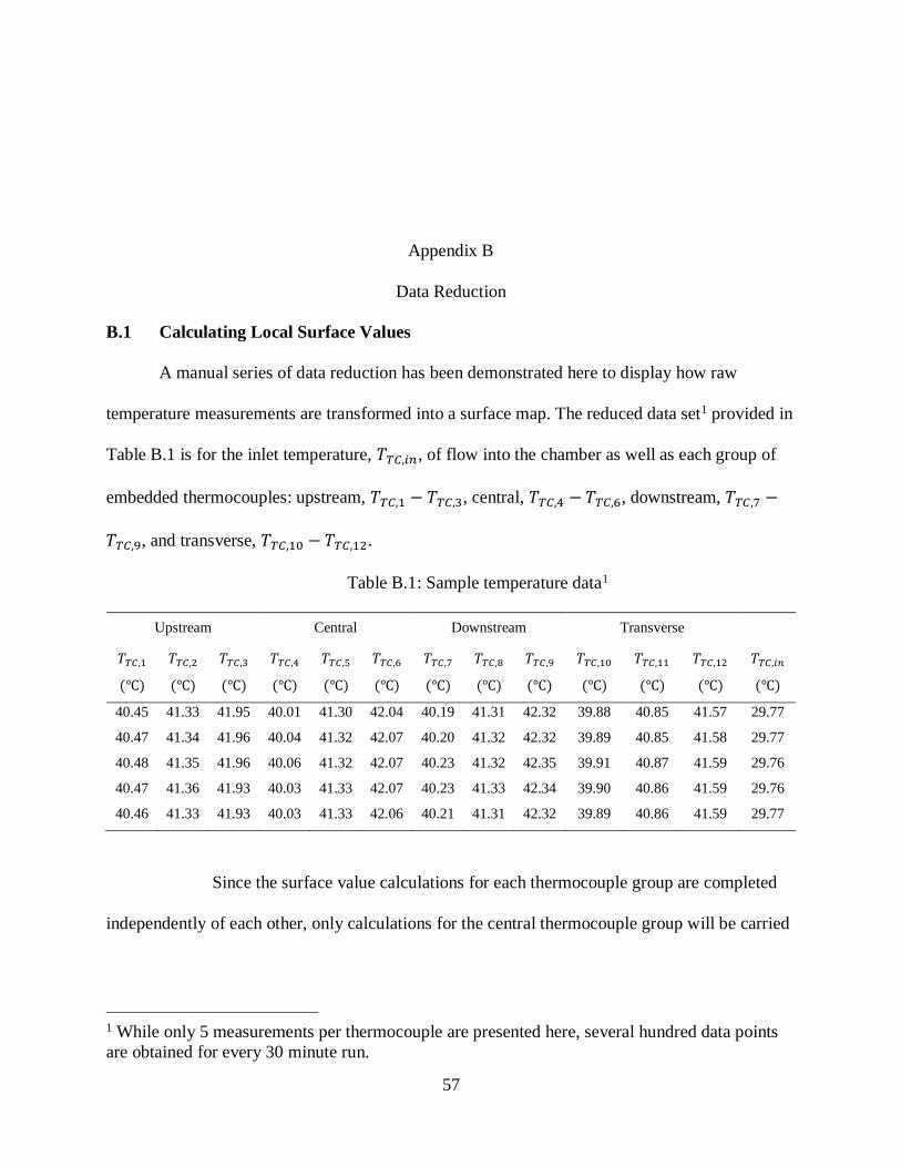
57

Appendix B

Data Reduction

B.1 Calculating Local Surface Values

A manual series of data reduction has been demonstrated here to display how raw

temperature measurements are transformed into a surface map. The reduced data set1 provided in

Table B.1 is for the inlet temperature, 𝑇𝑇𝐶,𝑖𝑛, of flow into the chamber as well as each group of

embedded thermocouples: upstream, 𝑇𝑇𝐶,1 − 𝑇𝑇𝐶,3, central, 𝑇𝑇𝐶,4 − 𝑇𝑇𝐶,6, downstream, 𝑇𝑇𝐶,7 −

𝑇𝑇𝐶,9, and transverse, 𝑇𝑇𝐶,10 − 𝑇𝑇𝐶,12.

Table B.1: Sample temperature data1

Upstream Central Downstream Transverse

𝑇𝑇𝐶,1

(℃)

𝑇𝑇𝐶,2

(℃)

𝑇𝑇𝐶,3

(℃)

𝑇𝑇𝐶,4

(℃)

𝑇𝑇𝐶,5

(℃)

𝑇𝑇𝐶,6

(℃)

𝑇𝑇𝐶,7

(℃)

𝑇𝑇𝐶,8

(℃)

𝑇𝑇𝐶,9

(℃)

𝑇𝑇𝐶,10

(℃)

𝑇𝑇𝐶,11

(℃)

𝑇𝑇𝐶,12

(℃)

𝑇𝑇𝐶,𝑖𝑛

(℃)

40.45 41.33 41.95 40.01 41.30 42.04 40.19 41.31 42.32 39.88 40.85 41.57 29.77

40.47 41.34 41.96 40.04 41.32 42.07 40.20 41.32 42.32 39.89 40.85 41.58 29.77

40.48 41.35 41.96 40.06 41.32 42.07 40.23 41.32 42.35 39.91 40.87 41.59 29.76

40.47 41.36 41.93 40.03 41.33 42.07 40.23 41.33 42.34 39.90 40.86 41.59 29.76

40.46 41.33 41.93 40.03 41.33 42.06 40.21 41.31 42.32 39.89 40.86 41.59 29.77

Since the surface value calculations for each thermocouple group are completed

independently of each other, only calculations for the central thermocouple group will be carried

1 While only 5 measurements per thermocouple are presented here, several hundred data points

are obtained for every 30 minute run.

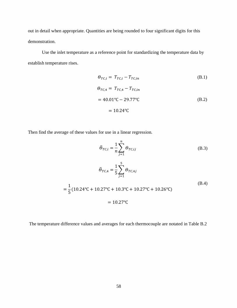
58

out in detail when appropriate. Quantities are being rounded to four significant digits for this

demonstration.

Use the inlet temperature as a reference point for standardizing the temperature data by

establish temperature rises.

𝛩𝑇𝐶,𝑖 = 𝑇𝑇𝐶,𝑖 − 𝑇𝑇𝐶,𝑖𝑛 (B.1)

𝛩𝑇𝐶,4 = 𝑇𝑇𝐶,4 − 𝑇𝑇𝐶,𝑖𝑛

= 40.01℃− 29.77℃

= 10.24℃

(B.2)

Then find the average of these values for use in a linear regression.

�̅�𝑇𝐶,𝑖 =

1

𝑛∑𝛩𝑇𝐶,𝑖𝑗

𝑛

𝑗=1

(B.3)

�̅�𝑇𝐶,4 =1

5∑𝛩𝑇𝐶,4𝑗

5

𝑗=1

=1

5(10.24℃ + 10.27℃+ 10.3℃+ 10.27℃+ 10.26℃)

= 10.27℃

(B.4)

The temperature difference values and averages for each thermocouple are notated in Table B.2

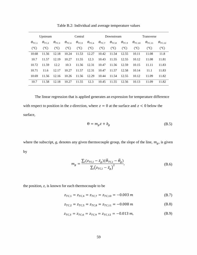
59

Table B.2: Individual and average temperature values

Upstream Central Downstream Transverse

𝛩𝑇𝐶,1

(℃)

𝛩𝑇𝐶,2

(℃)

𝛩𝑇𝐶,3

(℃)

𝛩𝑇𝐶,4

(℃)

𝛩𝑇𝐶,5

(℃)

𝛩𝑇𝐶,6

(℃)

𝛩𝑇𝐶,7

(℃)

𝛩𝑇𝐶,8

(℃)

𝛩𝑇𝐶,9

(℃)

𝛩𝑇𝐶,10

(℃)

𝛩𝑇𝐶,11

(℃)

𝛩𝑇𝐶,12

(℃)

10.68 11.56 12.18 10.24 11.53 12.27 10.42 11.54 12.55 10.11 11.08 11.8

10.7 11.57 12.19 10.27 11.55 12.3 10.43 11.55 12.55 10.12 11.08 11.81

10.72 11.59 12.2 10.3 11.56 12.31 10.47 11.56 12.59 10.15 11.11 11.83

10.71 11.6 12.17 10.27 11.57 12.31 10.47 11.57 12.58 10.14 11.1 11.83

10.69 11.56 12.16 10.26 11.56 12.29 10.44 11.54 12.55 10.12 11.09 11.82

10.7 11.58 12.18 10.27 11.55 12.3 10.45 11.55 12.56 10.13 11.09 11.82

The linear regression that is applied generates an expression for temperature difference

with respect to position in the z-direction, where 𝑧 = 0 at the surface and 𝑧 < 0 below the

surface,

Θ = 𝑚𝑔𝑧 + 𝑏𝑔 (B.5)

where the subscript, g, denotes any given thermocouple group, the slope of the line, 𝑚𝑔, is given

by

𝑚𝑔 =∑ (𝑧𝑇𝐶,𝑖 − �̅�𝑔)(�̅�𝑇𝐶,𝑖 − �̅�𝑔)𝑖

∑ (𝑧𝑇𝐶,𝑖 − �̅�𝑔)𝑖2 , (B.6)

the position, z, is known for each thermocouple to be

𝑧𝑇𝐶,1 = 𝑧𝑇𝐶,4 = 𝑧𝑇𝐶,7 = 𝑧𝑇𝐶,10 = −0.003 𝑚 (B.7)

𝑧𝑇𝐶,2 = 𝑧𝑇𝐶,5 = 𝑧𝑇𝐶,8 = 𝑧𝑇𝐶,11 = −0.008 𝑚 (B.8)

𝑧𝑇𝐶,3 = 𝑧𝑇𝐶,6 = 𝑧𝑇𝐶,9 = 𝑧𝑇𝐶,12 = −0.013 𝑚, (B.9)

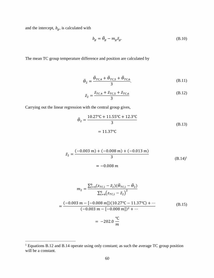
60

and the intercept, 𝑏𝑔, is calculated with

𝑏𝑔 = �̅�𝑔 −𝑚𝑔�̅�𝑔. (B.10)

The mean TC group temperature difference and position are calculated by

�̅�2 =�̅�𝑇𝐶,4 + �̅�𝑇𝐶,5 + �̅�𝑇𝐶,6

3. (B.11)

�̅�2 =

�̅�𝑇𝐶,4 + �̅�𝑇𝐶,5 + �̅�𝑇𝐶,63

(B.12)

Carrying out the linear regression with the central group gives,

�̅�2 =

10.27℃+ 11.55℃ + 12.3℃

3

= 11.37℃

(B.13)

�̅�2 =

(−0.003 𝑚) + (−0.008 𝑚) + (−0.013 𝑚)

3

= −0.008 𝑚

(B.14)1

𝑚2 =∑ (𝑧𝑇𝐶,𝑖 − �̅�2)(�̅�𝑇𝐶,𝑖 − �̅�2)6𝑖=4

∑ (𝑧𝑇𝐶,𝑖 − �̅�2)26

𝑖=4

=(−0.003 𝑚 − [−0.008 𝑚])(10.27℃− 11.37℃) +⋯

(−0.003 𝑚 − [−0.008 𝑚])2 +⋯

= −202.0 ℃

𝑚

(B.15)

1 Equations B.12 and B.14 operate using only constant; as such the average TC group position

will be a constant.

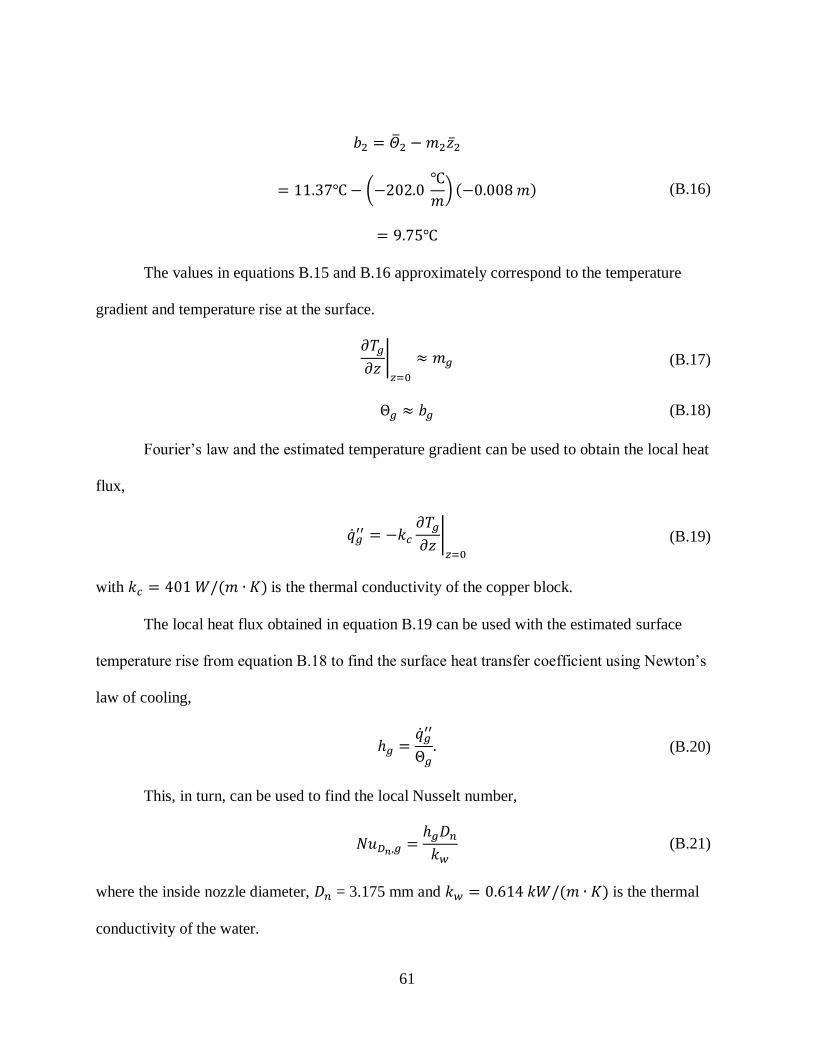
61

𝑏2 = �̅�2 −𝑚2�̅�2

= 11.37℃− (−202.0 ℃

𝑚)(−0.008 𝑚)

= 9.75℃

(B.16)

The values in equations B.15 and B.16 approximately correspond to the temperature

gradient and temperature rise at the surface.

𝜕𝑇𝑔𝜕𝑧|𝑧=0

≈ 𝑚𝑔 (B.17)

Θ𝑔 ≈ 𝑏𝑔 (B.18)

Fourier’s law and the estimated temperature gradient can be used to obtain the local heat

flux,

�̇�𝑔′′ = −𝑘𝑐

𝜕𝑇𝑔𝜕𝑧|𝑧=0

(B.19)

with 𝑘𝑐 = 401 𝑊/(𝑚 ∙ 𝐾) is the thermal conductivity of the copper block.

The local heat flux obtained in equation B.19 can be used with the estimated surface

temperature rise from equation B.18 to find the surface heat transfer coefficient using Newton’s

law of cooling,

ℎ𝑔 =�̇�𝑔′′

Θ𝑔. (B.20)

This, in turn, can be used to find the local Nusselt number,

𝑁𝑢𝐷𝑛,𝑔 =ℎ𝑔𝐷𝑛𝑘𝑤

(B.21)

where the inside nozzle diameter, 𝐷𝑛 = 3.175 mm and 𝑘𝑤 = 0.614 𝑘𝑊/(𝑚 ∙ 𝐾) is the thermal

conductivity of the water.

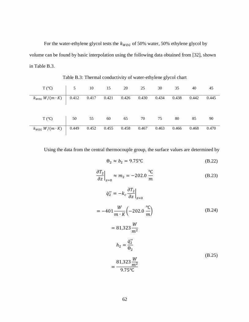
62

For the water-ethylene glycol tests the 𝑘𝑊𝐸𝐺 of 50% water, 50% ethylene glycol by

volume can be found by basic interpolation using the following data obtained from [32], shown

in Table B.3.

Table B.3: Thermal conductivity of water-ethylene glycol chart

T (℃) 5 10 15 20 25 30 35 40 45

𝑘𝑊𝐸𝐺 𝑊/(𝑚 ∙ 𝐾) 0.412 0.417 0.421 0.426 0.430 0.434 0.438 0.442 0.445

T (℃) 50 55 60 65 70 75 80 85 90

𝑘𝑊𝐸𝐺 𝑊/(𝑚 ∙ 𝐾) 0.449 0.452 0.455 0.458 0.467 0.463 0.466 0.468 0.470

Using the data from the central thermocouple group, the surface values are determined by

Θ2 ≈ 𝑏2 = 9.75℃ (B.22)

𝜕𝑇2𝜕𝑧|𝑧=0

≈ 𝑚2 = −202.0 ℃

𝑚 (B.23)

�̇�2′′ = −𝑘𝑐

𝜕𝑇2𝜕𝑧|𝑧=0

= −401𝑊

𝑚 ∙ 𝐾(−202.0

℃

𝑚)

= 81,323𝑊

𝑚2

(B.24)

ℎ2 =�̇�2′′

Θ2

=81,323

𝑊𝑚2

9.75℃

(B.25)

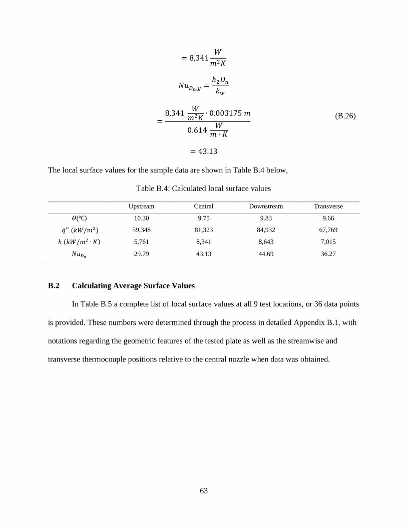
63

= 8,341𝑊

𝑚2𝐾

𝑁𝑢𝐷𝑛 ,𝑔 =ℎ2𝐷𝑛𝑘𝑤

=8,341

𝑊𝑚2𝐾

∙ 0.003175 𝑚

0.614 𝑊𝑚 ∙ 𝐾

= 43.13

(B.26)

The local surface values for the sample data are shown in Table B.4 below,

Table B.4: Calculated local surface values

Upstream Central Downstream Transverse

𝛩(℃) 10.30 9.75 9.83 9.66

�̇�′′ (𝑘𝑊/𝑚2) 59,348 81,323 84,932 67,769

ℎ (𝑘𝑊/𝑚2 ∙ 𝐾) 5,761 8,341 8,643 7,015

𝑁𝑢𝐷𝑛 29.79 43.13 44.69 36.27

B.2 Calculating Average Surface Values

In Table B.5 a complete list of local surface values at all 9 test locations, or 36 data points

is provided. These numbers were determined through the process in detailed Appendix B.1, with

notations regarding the geometric features of the tested plate as well as the streamwise and

transverse thermocouple positions relative to the central nozzle when data was obtained.

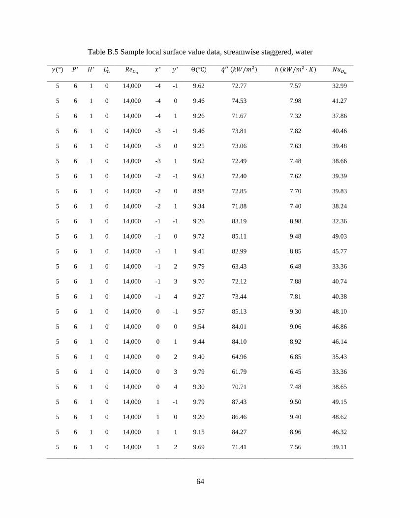
64

Table B.5 Sample local surface value data, streamwise staggered, water

𝛾(°) 𝑃∗ 𝐻∗ 𝐿𝑛∗ 𝑅𝑒𝐷𝑛 𝑥∗ 𝑦∗ Θ(℃) �̇�′′ (𝑘𝑊/𝑚2) ℎ (𝑘𝑊/𝑚2 ∙ 𝐾) 𝑁𝑢𝐷𝑛

5 6 1 0 14,000 -4 -1 9.62 72.77 7.57 32.99

5 6 1 0 14,000 -4 0 9.46 74.53 7.98 41.27

5 6 1 0 14,000 -4 1 9.26 71.67 7.32 37.86

5 6 1 0 14,000 -3 -1 9.46 73.81 7.82 40.46

5 6 1 0 14,000 -3 0 9.25 73.06 7.63 39.48

5 6 1 0 14,000 -3 1 9.62 72.49 7.48 38.66

5 6 1 0 14,000 -2 -1 9.63 72.40 7.62 39.39

5 6 1 0 14,000 -2 0 8.98 72.85 7.70 39.83

5 6 1 0 14,000 -2 1 9.34 71.88 7.40 38.24

5 6 1 0 14,000 -1 -1 9.26 83.19 8.98 32.36

5 6 1 0 14,000 -1 0 9.72 85.11 9.48 49.03

5 6 1 0 14,000 -1 1 9.41 82.99 8.85 45.77

5 6 1 0 14,000 -1 2 9.79 63.43 6.48 33.36

5 6 1 0 14,000 -1 3 9.70 72.12 7.88 40.74

5 6 1 0 14,000 -1 4 9.27 73.44 7.81 40.38

5 6 1 0 14,000 0 -1 9.57 85.13 9.30 48.10

5 6 1 0 14,000 0 0 9.54 84.01 9.06 46.86

5 6 1 0 14,000 0 1 9.44 84.10 8.92 46.14

5 6 1 0 14,000 0 2 9.40 64.96 6.85 35.43

5 6 1 0 14,000 0 3 9.79 61.79 6.45 33.36

5 6 1 0 14,000 0 4 9.30 70.71 7.48 38.65

5 6 1 0 14,000 1 -1 9.79 87.43 9.50 49.15

5 6 1 0 14,000 1 0 9.20 86.46 9.40 48.62

5 6 1 0 14,000 1 1 9.15 84.27 8.96 46.32

5 6 1 0 14,000 1 2 9.69 71.41 7.56 39.11

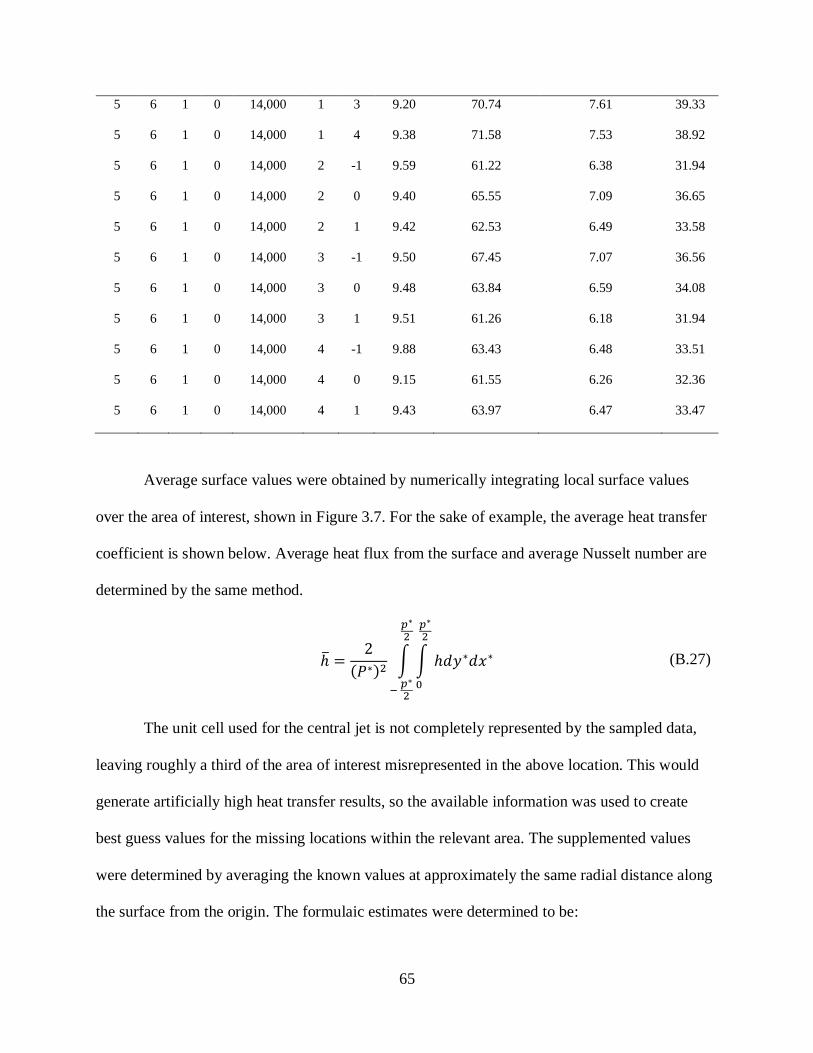
65

5 6 1 0 14,000 1 3 9.20 70.74 7.61 39.33

5 6 1 0 14,000 1 4 9.38 71.58 7.53 38.92

5 6 1 0 14,000 2 -1 9.59 61.22 6.38 31.94

5 6 1 0 14,000 2 0 9.40 65.55 7.09 36.65

5 6 1 0 14,000 2 1 9.42 62.53 6.49 33.58

5 6 1 0 14,000 3 -1 9.50 67.45 7.07 36.56

5 6 1 0 14,000 3 0 9.48 63.84 6.59 34.08

5 6 1 0 14,000 3 1 9.51 61.26 6.18 31.94

5 6 1 0 14,000 4 -1 9.88 63.43 6.48 33.51

5 6 1 0 14,000 4 0 9.15 61.55 6.26 32.36

5 6 1 0 14,000 4 1 9.43 63.97 6.47 33.47

Average surface values were obtained by numerically integrating local surface values

over the area of interest, shown in Figure 3.7. For the sake of example, the average heat transfer

coefficient is shown below. Average heat flux from the surface and average Nusselt number are

determined by the same method.

ℎ̅ =2

(𝑃∗)2∫ ∫ ℎ𝑑𝑦∗𝑑𝑥∗

𝑝∗

2

0

𝑝∗

2

− 𝑝∗

2

(B.27)

The unit cell used for the central jet is not completely represented by the sampled data,

leaving roughly a third of the area of interest misrepresented in the above location. This would

generate artificially high heat transfer results, so the available information was used to create

best guess values for the missing locations within the relevant area. The supplemented values

were determined by averaging the known values at approximately the same radial distance along

the surface from the origin. The formulaic estimates were determined to be:

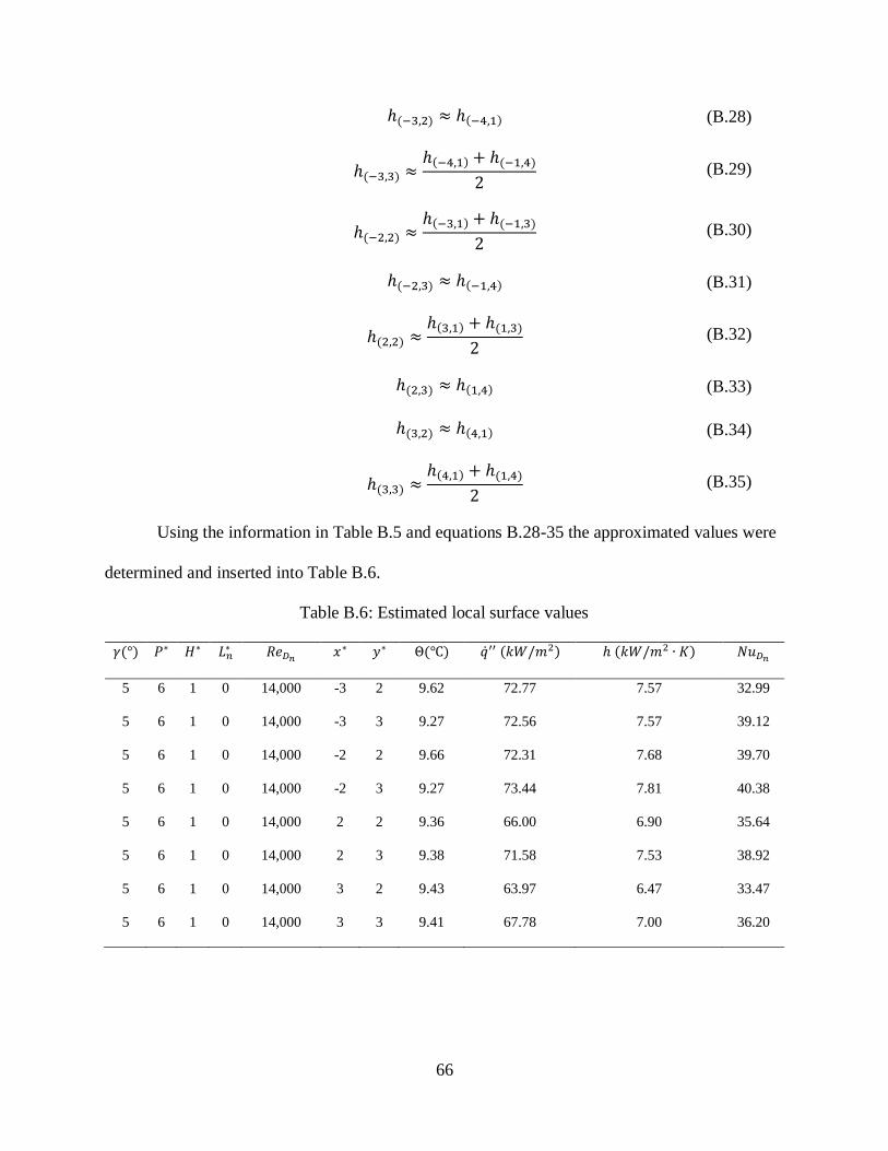
66

ℎ(−3,2) ≈ ℎ(−4,1) (B.28)

ℎ(−3,3) ≈ℎ(−4,1) + ℎ(−1,4)

2 (B.29)

ℎ(−2,2) ≈ℎ(−3,1) + ℎ(−1,3)

2 (B.30)

ℎ(−2,3) ≈ ℎ(−1,4) (B.31)

ℎ(2,2) ≈ℎ(3,1) + ℎ(1,3)

2 (B.32)

ℎ(2,3) ≈ ℎ(1,4) (B.33)

ℎ(3,2) ≈ ℎ(4,1) (B.34)

ℎ(3,3) ≈ℎ(4,1) + ℎ(1,4)

2 (B.35)

Using the information in Table B.5 and equations B.28-35 the approximated values were

determined and inserted into Table B.6.

Table B.6: Estimated local surface values

𝛾(°) 𝑃∗ 𝐻∗ 𝐿𝑛∗ 𝑅𝑒𝐷𝑛 𝑥∗ 𝑦∗ Θ(℃) �̇�′′ (𝑘𝑊/𝑚2) ℎ (𝑘𝑊/𝑚2 ∙ 𝐾) 𝑁𝑢𝐷𝑛

5 6 1 0 14,000 -3 2 9.62 72.77 7.57 32.99

5 6 1 0 14,000 -3 3 9.27 72.56 7.57 39.12

5 6 1 0 14,000 -2 2 9.66 72.31 7.68 39.70

5 6 1 0 14,000 -2 3 9.27 73.44 7.81 40.38

5 6 1 0 14,000 2 2 9.36 66.00 6.90 35.64

5 6 1 0 14,000 2 3 9.38 71.58 7.53 38.92

5 6 1 0 14,000 3 2 9.43 63.97 6.47 33.47

5 6 1 0 14,000 3 3 9.41 67.78 7.00 36.20

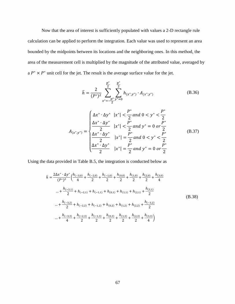
67

Now that the area of interest is sufficiently populated with values a 2-D rectangle rule

calculation can be applied to perform the integration. Each value was used to represent an area

bounded by the midpoints between its locations and the neighboring ones. In this method, the

area of the measurement cell is multiplied by the magnitude of the attributed value, averaged by

a 𝑃∗ × 𝑃∗ unit cell for the jet. The result is the average surface value for the jet.

ℎ̅ =2

(𝑃∗)2∑ ∑ ℎ(𝑥∗,𝑦∗) ∙ 𝐴(𝑥∗,𝑦∗)

𝑝∗

2

𝑦∗=0

𝑝∗

2

𝑥∗=−𝑝∗

2

(B.36)

𝐴(𝑥∗,𝑦∗) =

{

Δ𝑥∗ ∙ Δ𝑦∗ |𝑥∗| <

𝑃∗

2𝑎𝑛𝑑 0 < 𝑦∗ <

𝑃∗

2Δ𝑥∗ ∙ Δ𝑦∗

2 |𝑥∗| <

𝑃∗

2𝑎𝑛𝑑 𝑦∗ = 0 𝑜𝑟

𝑃∗

2Δ𝑥∗ ∙ Δ𝑦∗

2 |𝑥∗| =

𝑃∗

2𝑎𝑛𝑑 0 < 𝑦∗ <

𝑃∗

2Δ𝑥∗ ∙ Δ𝑦∗

2 |𝑥∗| =

𝑃∗

2𝑎𝑛𝑑 𝑦∗ = 0 𝑜𝑟

𝑃∗

2

(B.37)

Using the data provided in Table B.5, the integration is conducted below as

ℎ̅ =2Δ𝑥∗ ∙ Δ𝑦∗

(𝑃∗)2(ℎ(−3,0)4

+ℎ(−2,0)2

+ℎ(−1,0)2

+ℎ(0,0)2

+ℎ(1,0)2

+ℎ(2,0)2

+ℎ(3,0)4

…+ℎ(−3,1)2

+ ℎ(−2,1) + ℎ(−1,1) + ℎ(0,1) + ℎ(1,1) + ℎ(2,1) +ℎ(3,1)2

…+ℎ(−3,2)2

+ ℎ(−2,2) + ℎ(−1,2) + ℎ(0,2) + ℎ(1,2) + ℎ(2,2) +ℎ(−3,2)2

…+ℎ(−3,3)4

+ℎ(−2,3)2

+ℎ(−1,3)2

+ℎ(0,3)2

+ℎ(1,3)2

+ℎ(2,3)2

+ℎ(3,3)4

)

(B.38)

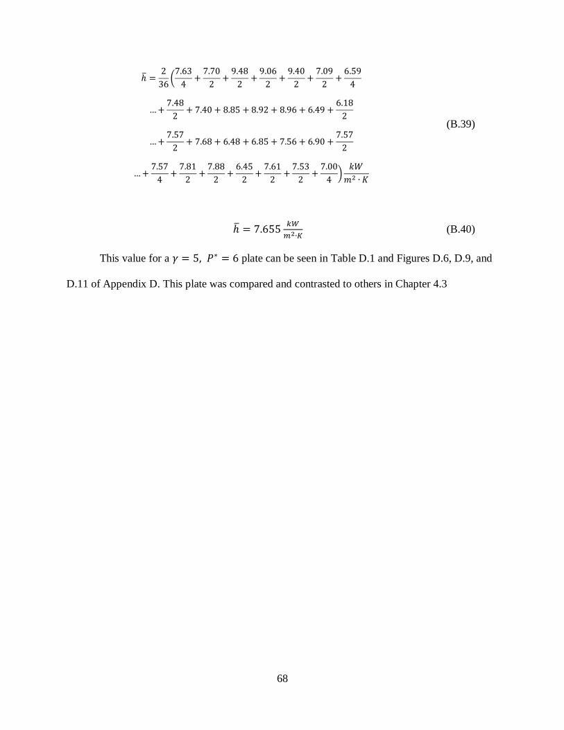
68

ℎ̅ =2

36(7.63

4+7.70

2+9.48

2+9.06

2+9.40

2+7.09

2+6.59

4

…+7.48

2+ 7.40 + 8.85 + 8.92 + 8.96 + 6.49 +

6.18

2

…+7.57

2+ 7.68 + 6.48 + 6.85 + 7.56 + 6.90 +

7.57

2

…+7.57

4+7.81

2+7.88

2+6.45

2+7.61

2+7.53

2+7.00

4)𝑘𝑊

𝑚2 ∙ 𝐾

(B.39)

ℎ̅ = 7.655 𝑘𝑊

𝑚2∙𝐾 (B.40)

This value for a 𝛾 = 5, 𝑃∗ = 6 plate can be seen in Table D.1 and Figures D.6, D.9, and

D.11 of Appendix D. This plate was compared and contrasted to others in Chapter 4.3

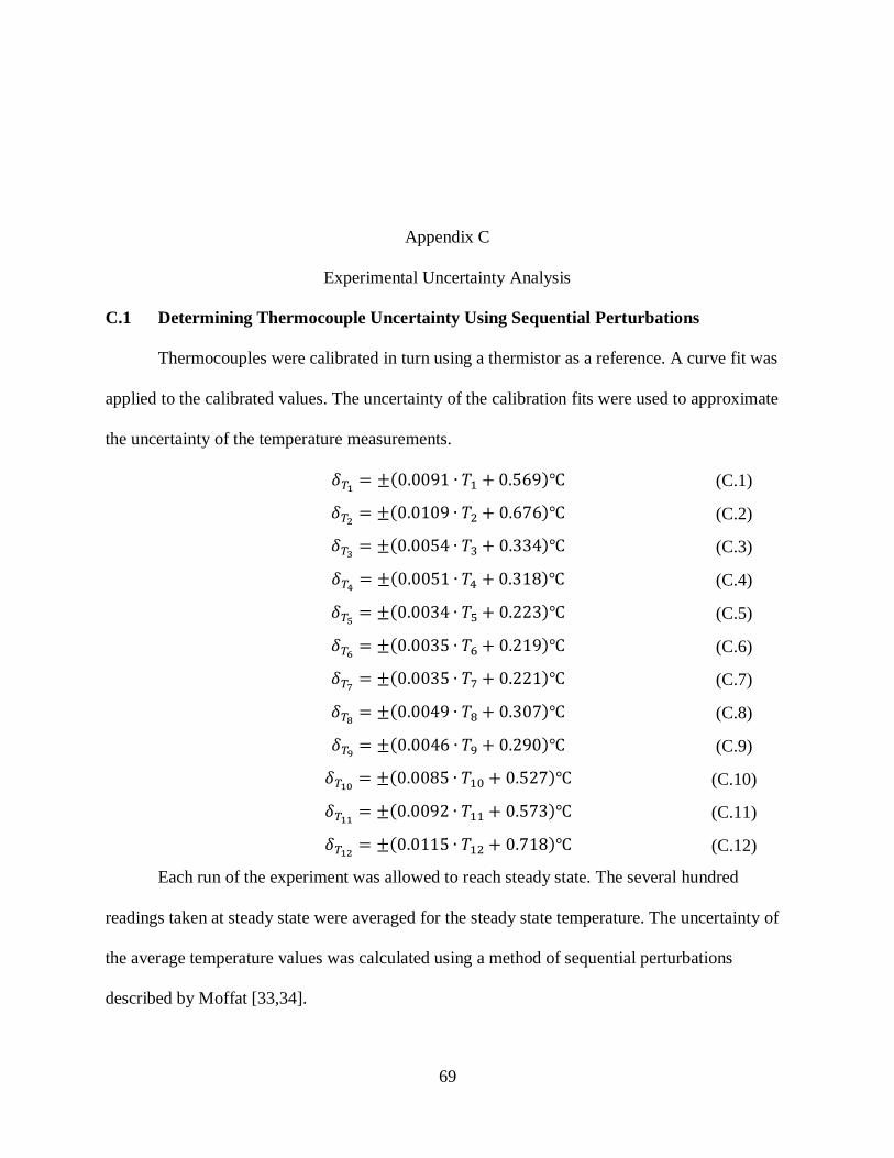
69

Appendix C

Experimental Uncertainty Analysis

C.1 Determining Thermocouple Uncertainty Using Sequential Perturbations

Thermocouples were calibrated in turn using a thermistor as a reference. A curve fit was

applied to the calibrated values. The uncertainty of the calibration fits were used to approximate

the uncertainty of the temperature measurements.

𝛿𝑇1 = ±(0.0091 ∙ 𝑇1 + 0.569)℃ (C.1)

𝛿𝑇2 = ±(0.0109 ∙ 𝑇2 + 0.676)℃ (C.2)

𝛿𝑇3 = ±(0.0054 ∙ 𝑇3 + 0.334)℃ (C.3)

𝛿𝑇4 = ±(0.0051 ∙ 𝑇4 + 0.318)℃ (C.4)

𝛿𝑇5 = ±(0.0034 ∙ 𝑇5 + 0.223)℃ (C.5)

𝛿𝑇6 = ±(0.0035 ∙ 𝑇6 + 0.219)℃ (C.6)

𝛿𝑇7 = ±(0.0035 ∙ 𝑇7 + 0.221)℃ (C.7)

𝛿𝑇8 = ±(0.0049 ∙ 𝑇8 + 0.307)℃ (C.8)

𝛿𝑇9 = ±(0.0046 ∙ 𝑇9 + 0.290)℃ (C.9)

𝛿𝑇10 = ±(0.0085 ∙ 𝑇10 + 0.527)℃ (C.10)

𝛿𝑇11 = ±(0.0092 ∙ 𝑇11 + 0.573)℃ (C.11)

𝛿𝑇12 = ±(0.0115 ∙ 𝑇12 + 0.718)℃ (C.12)

Each run of the experiment was allowed to reach steady state. The several hundred

readings taken at steady state were averaged for the steady state temperature. The uncertainty of

the average temperature values was calculated using a method of sequential perturbations

described by Moffat [33,34].

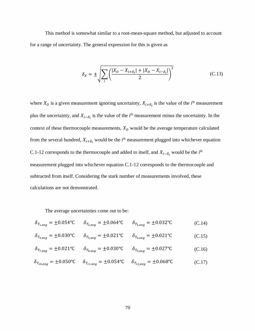
70

This method is somewhat similar to a root-mean-square method, but adjusted to account

for a range of uncertainty. The general expression for this is given as

𝛿𝑋 = ±√∑(|𝑋𝑂 − 𝑋𝑖+𝛿𝑖| + |𝑋𝑂 − 𝑋𝑖−𝛿𝑖|

2)

2

𝑖

(C.13)

where 𝑋𝑂 is a given measurement ignoring uncertainty, 𝑋𝑖+𝛿𝑖 is the value of the ith measurement

plus the uncertainty, and 𝑋𝑖−𝛿𝑖 is the value of the ith measurement minus the uncertainty. In the

context of these thermocouple measurements, 𝑋𝑂 would be the average temperature calculated

from the several hundred, 𝑋𝑖+𝛿𝑖 would be the ith measurement plugged into whichever equation

C.1-12 corresponds to the thermocouple and added to itself, and 𝑋𝑖−𝛿𝑖 would be the ith

measurement plugged into whichever equation C.1-12 corresponds to the thermocouple and

subtracted from itself. Considering the stark number of measurements involved, these

calculations are not demonstrated.

The average uncertainties come out to be:

𝛿𝑇1,𝑎𝑣𝑔 = ±0.054℃ 𝛿𝑇2,𝑎𝑣𝑔 = ±0.064℃ 𝛿𝑇3,𝑎𝑣𝑔 = ±0.032℃ (C.14)

𝛿𝑇4,𝑎𝑣𝑔 = ±0.030℃ 𝛿𝑇5,𝑎𝑣𝑔 = ±0.021℃ 𝛿𝑇6,𝑎𝑣𝑔 = ±0.021℃ (C.15)

𝛿𝑇7,𝑎𝑣𝑔 = ±0.021℃ 𝛿𝑇8,𝑎𝑣𝑔 = ±0.030℃ 𝛿𝑇9,𝑎𝑣𝑔 = ±0.027℃ (C.16)

𝛿𝑇10,𝑎𝑣𝑔 = ±0.050℃ 𝛿𝑇11,𝑎𝑣𝑔 = ±0.054℃ 𝛿𝑇12,𝑎𝑣𝑔 = ±0.068℃ (C.17)

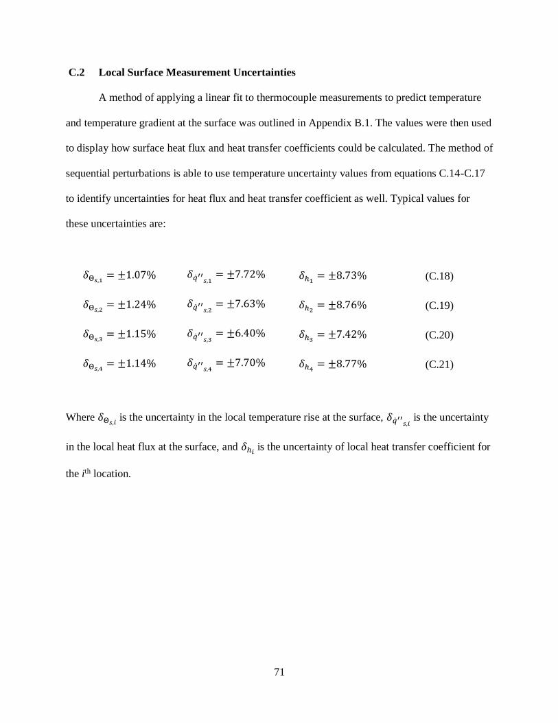
71

C.2 Local Surface Measurement Uncertainties

A method of applying a linear fit to thermocouple measurements to predict temperature

and temperature gradient at the surface was outlined in Appendix B.1. The values were then used

to display how surface heat flux and heat transfer coefficients could be calculated. The method of

sequential perturbations is able to use temperature uncertainty values from equations C.14-C.17

to identify uncertainties for heat flux and heat transfer coefficient as well. Typical values for

these uncertainties are:

𝛿Θ𝑠,1 = ±1.07% 𝛿�̇�′′𝑠,1 = ±7.72% 𝛿ℎ1 = ±8.73% (C.18)

𝛿Θ𝑠,2 = ±1.24% 𝛿�̇�′′𝑠,2 = ±7.63% 𝛿ℎ2 = ±8.76% (C.19)

𝛿Θ𝑠,3 = ±1.15% 𝛿�̇�′′𝑠,3 = ±6.40% 𝛿ℎ3 = ±7.42% (C.20)

𝛿Θ𝑠,4 = ±1.14% 𝛿�̇�′′𝑠,4 = ±7.70% 𝛿ℎ4 = ±8.77% (C.21)

Where 𝛿Θ𝑠,𝑖 is the uncertainty in the local temperature rise at the surface, 𝛿�̇�′′𝑠,𝑖 is the uncertainty

in the local heat flux at the surface, and 𝛿ℎ𝑖 is the uncertainty of local heat transfer coefficient for

the ith location.

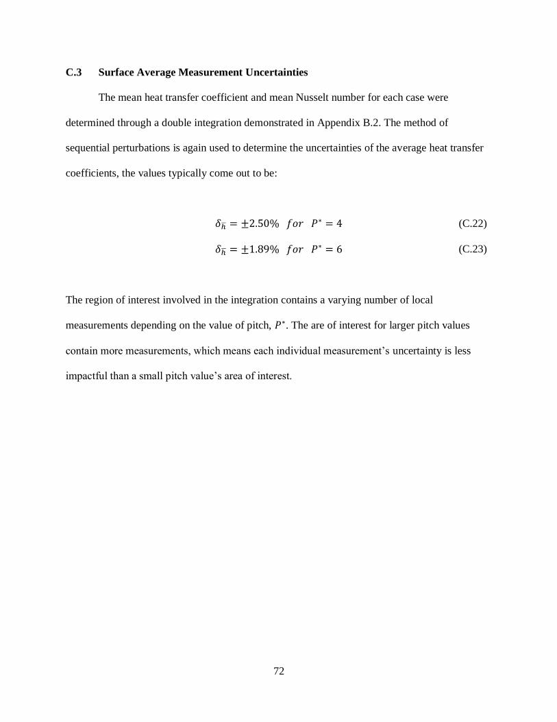
72

C.3 Surface Average Measurement Uncertainties

The mean heat transfer coefficient and mean Nusselt number for each case were

determined through a double integration demonstrated in Appendix B.2. The method of

sequential perturbations is again used to determine the uncertainties of the average heat transfer

coefficients, the values typically come out to be:

𝛿ℎ̅ = ±2.50% 𝑓𝑜𝑟 𝑃∗ = 4 (C.22)

𝛿ℎ̅ = ±1.89% 𝑓𝑜𝑟 𝑃∗ = 6 (C.23)

The region of interest involved in the integration contains a varying number of local

measurements depending on the value of pitch, 𝑃∗. The are of interest for larger pitch values

contain more measurements, which means each individual measurement’s uncertainty is less

impactful than a small pitch value’s area of interest.

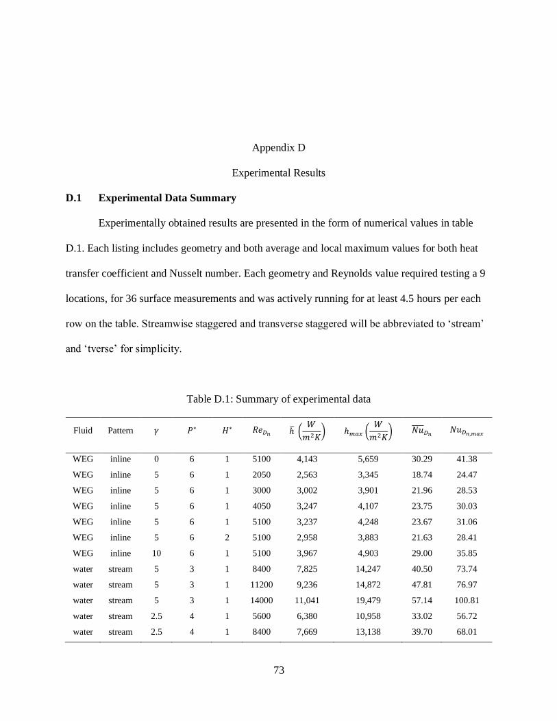
73

Appendix D

Experimental Results

D.1 Experimental Data Summary

Experimentally obtained results are presented in the form of numerical values in table

D.1. Each listing includes geometry and both average and local maximum values for both heat

transfer coefficient and Nusselt number. Each geometry and Reynolds value required testing a 9

locations, for 36 surface measurements and was actively running for at least 4.5 hours per each

row on the table. Streamwise staggered and transverse staggered will be abbreviated to ‘stream’

and ‘tverse’ for simplicity.

Table D.1: Summary of experimental data

Fluid Pattern 𝛾 𝑃∗ 𝐻∗ 𝑅𝑒𝐷𝑛 ℎ̅ (𝑊

𝑚2𝐾) ℎ𝑚𝑎𝑥 (

𝑊

𝑚2𝐾) 𝑁𝑢̅̅ ̅̅ 𝐷𝑛 𝑁𝑢𝐷𝑛,𝑚𝑎𝑥

WEG inline 0 6 1 5100 4,143 5,659 30.29 41.38

WEG inline 5 6 1 2050 2,563 3,345 18.74 24.47

WEG inline 5 6 1 3000 3,002 3,901 21.96 28.53

WEG inline 5 6 1 4050 3,247 4,107 23.75 30.03

WEG inline 5 6 1 5100 3,237 4,248 23.67 31.06

WEG inline 5 6 2 5100 2,958 3,883 21.63 28.41

WEG inline 10 6 1 5100 3,967 4,903 29.00 35.85

water stream 5 3 1 8400 7,825 14,247 40.50 73.74

water stream 5 3 1 11200 9,236 14,872 47.81 76.97

water stream 5 3 1 14000 11,041 19,479 57.14 100.81

water stream 2.5 4 1 5600 6,380 10,958 33.02 56.72

water stream 2.5 4 1 8400 7,669 13,138 39.70 68.01

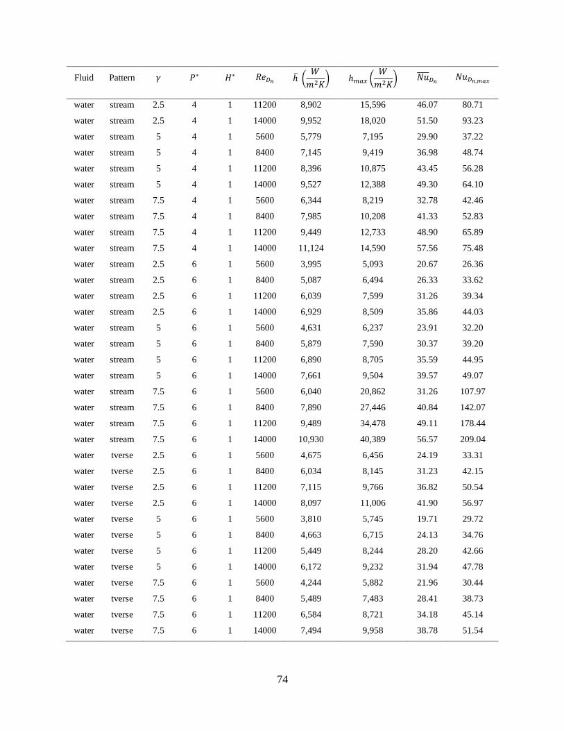
74

Fluid Pattern 𝛾 𝑃∗ 𝐻∗ 𝑅𝑒𝐷𝑛 ℎ̅ (𝑊

𝑚2𝐾) ℎ𝑚𝑎𝑥 (

𝑊

𝑚2𝐾) 𝑁𝑢̅̅ ̅̅ 𝐷𝑛 𝑁𝑢𝐷𝑛,𝑚𝑎𝑥

water stream 2.5 4 1 11200 8,902 15,596 46.07 80.71

water stream 2.5 4 1 14000 9,952 18,020 51.50 93.23

water stream 5 4 1 5600 5,779 7,195 29.90 37.22

water stream 5 4 1 8400 7,145 9,419 36.98 48.74

water stream 5 4 1 11200 8,396 10,875 43.45 56.28

water stream 5 4 1 14000 9,527 12,388 49.30 64.10

water stream 7.5 4 1 5600 6,344 8,219 32.78 42.46

water stream 7.5 4 1 8400 7,985 10,208 41.33 52.83

water stream 7.5 4 1 11200 9,449 12,733 48.90 65.89

water stream 7.5 4 1 14000 11,124 14,590 57.56 75.48

water stream 2.5 6 1 5600 3,995 5,093 20.67 26.36

water stream 2.5 6 1 8400 5,087 6,494 26.33 33.62

water stream 2.5 6 1 11200 6,039 7,599 31.26 39.34

water stream 2.5 6 1 14000 6,929 8,509 35.86 44.03

water stream 5 6 1 5600 4,631 6,237 23.91 32.20

water stream 5 6 1 8400 5,879 7,590 30.37 39.20

water stream 5 6 1 11200 6,890 8,705 35.59 44.95

water stream 5 6 1 14000 7,661 9,504 39.57 49.07

water stream 7.5 6 1 5600 6,040 20,862 31.26 107.97

water stream 7.5 6 1 8400 7,890 27,446 40.84 142.07

water stream 7.5 6 1 11200 9,489 34,478 49.11 178.44

water stream 7.5 6 1 14000 10,930 40,389 56.57 209.04

water tverse 2.5 6 1 5600 4,675 6,456 24.19 33.31

water tverse 2.5 6 1 8400 6,034 8,145 31.23 42.15

water tverse 2.5 6 1 11200 7,115 9,766 36.82 50.54

water tverse 2.5 6 1 14000 8,097 11,006 41.90 56.97

water tverse 5 6 1 5600 3,810 5,745 19.71 29.72

water tverse 5 6 1 8400 4,663 6,715 24.13 34.76

water tverse 5 6 1 11200 5,449 8,244 28.20 42.66

water tverse 5 6 1 14000 6,172 9,232 31.94 47.78

water tverse 7.5 6 1 5600 4,244 5,882 21.96 30.44

water tverse 7.5 6 1 8400 5,489 7,483 28.41 38.73

water tverse 7.5 6 1 11200 6,584 8,721 34.18 45.14

water tverse 7.5 6 1 14000 7,494 9,958 38.78 51.54

75

D.2 Experimental Surface Maps

Provided below surface maps generated from local values of experimentally obtained

heat transfer data.

• Figures D.1-D.3 display results for water-ethylene glycol results at varying flow rates and

geometric parameters.

• Figures D.4 – D.7 display results for staggered arrays at the three largest Reynolds

numbers for 𝛾 = 5° of each staggered geometry tested.

• Figure D.8 displays results for 𝛾 = 5° for each pitch value of streamwise staggered plate.

• Figure D.9 displays results for 𝛾 = 5°, 𝑃∗ = 6 for both streamwise and transverse

staggered plates.

• Figures D.10-D.12 display results for staggered arrays with varying angle for the three

patterns tested at all three angles.

• Figure D.13 displays results for staggered arrays with varying Reynolds numbers for 𝛾 =

5°, 𝑃∗ = 6 to demonstrate skewed results just downstream of center. The plate was tested

twice with intermediating tests between, showing no concerning results. Only the more

recent set of acquired data for this geometry is presented in this study

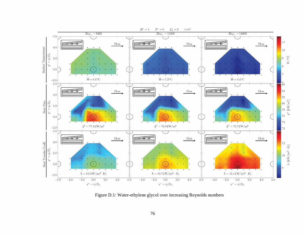
76

Figure D.1: Water-ethylene glycol over increasing Reynolds numbers

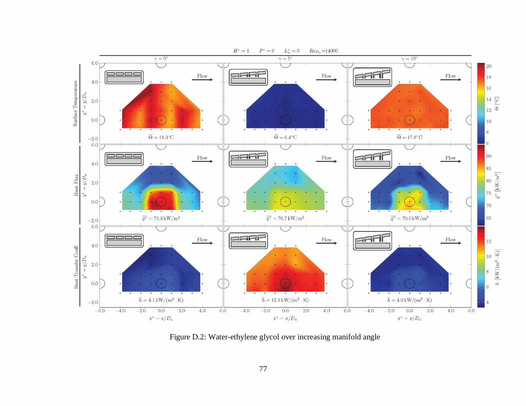
77

Figure D.2: Water-ethylene glycol over increasing manifold angle

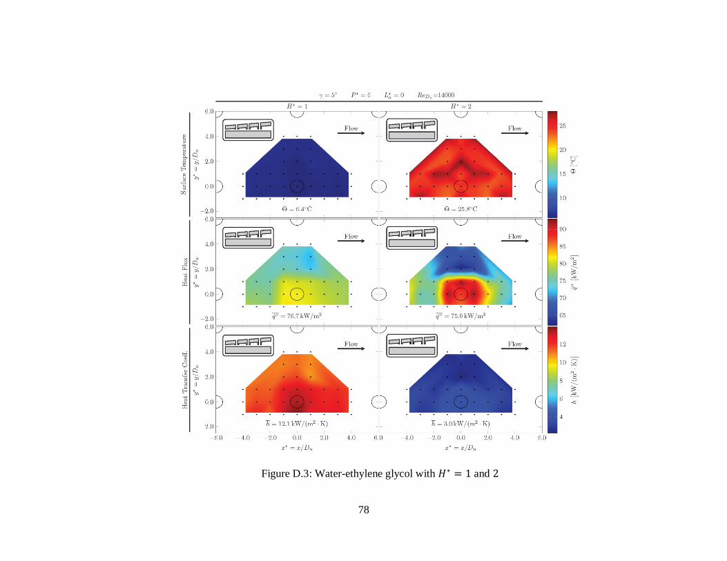
78

Figure D.3: Water-ethylene glycol with 𝐻∗ = 1 and 2

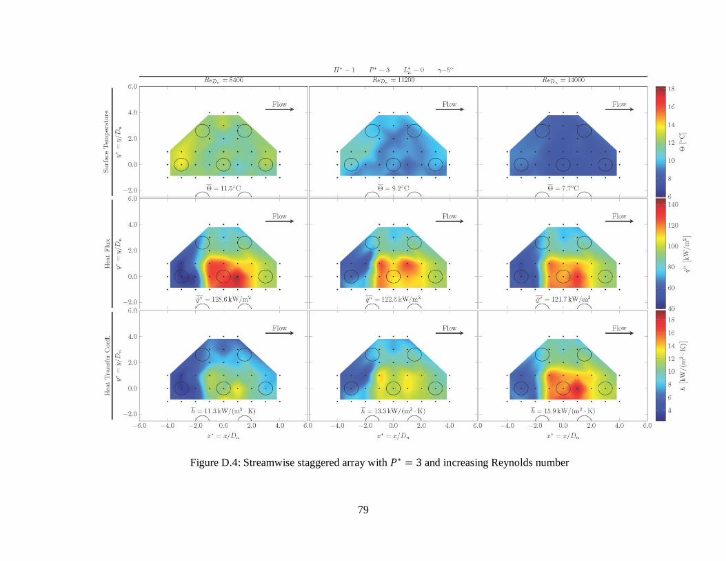
79

Figure D.4: Streamwise staggered array with 𝑃∗ = 3 and increasing Reynolds number

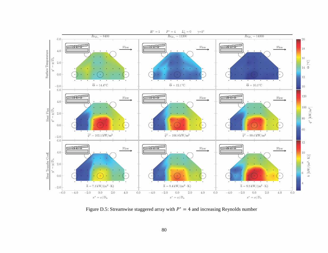
80

Figure D.5: Streamwise staggered array with 𝑃∗ = 4 and increasing Reynolds number

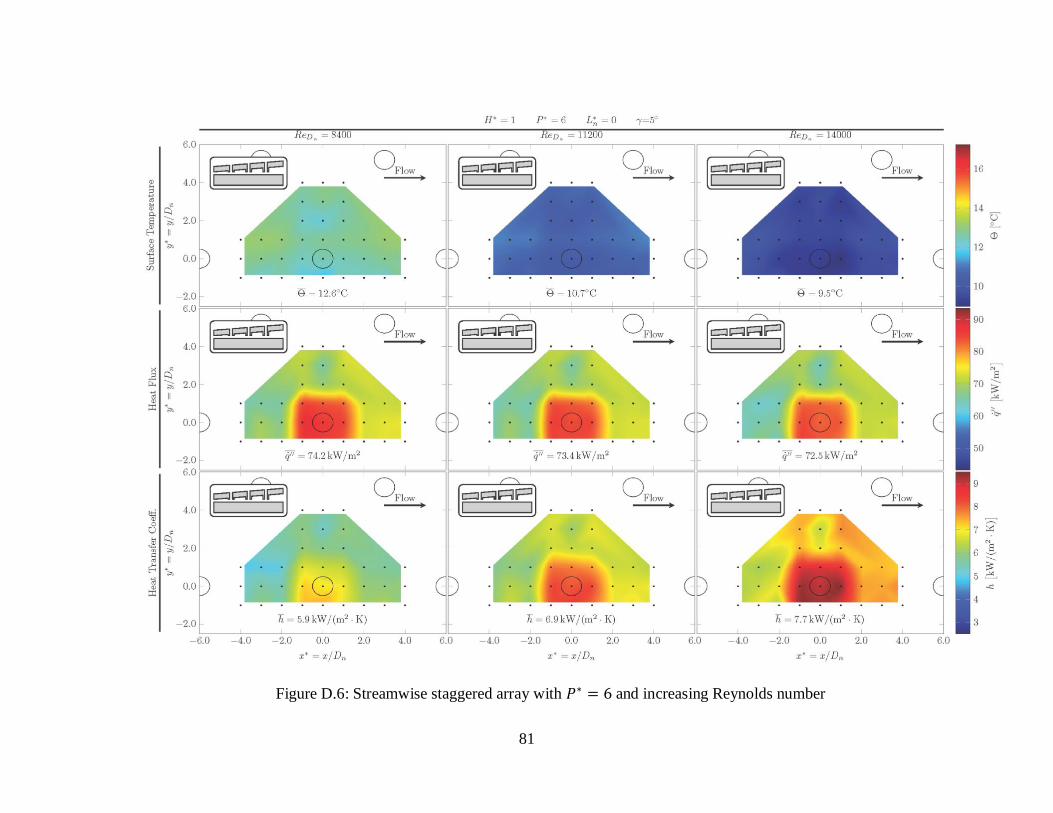
81

Figure D.6: Streamwise staggered array with 𝑃∗ = 6 and increasing Reynolds number

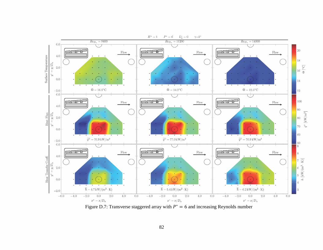
82

Figure D.7: Transverse staggered array with 𝑃∗ = 6 and increasing Reynolds number

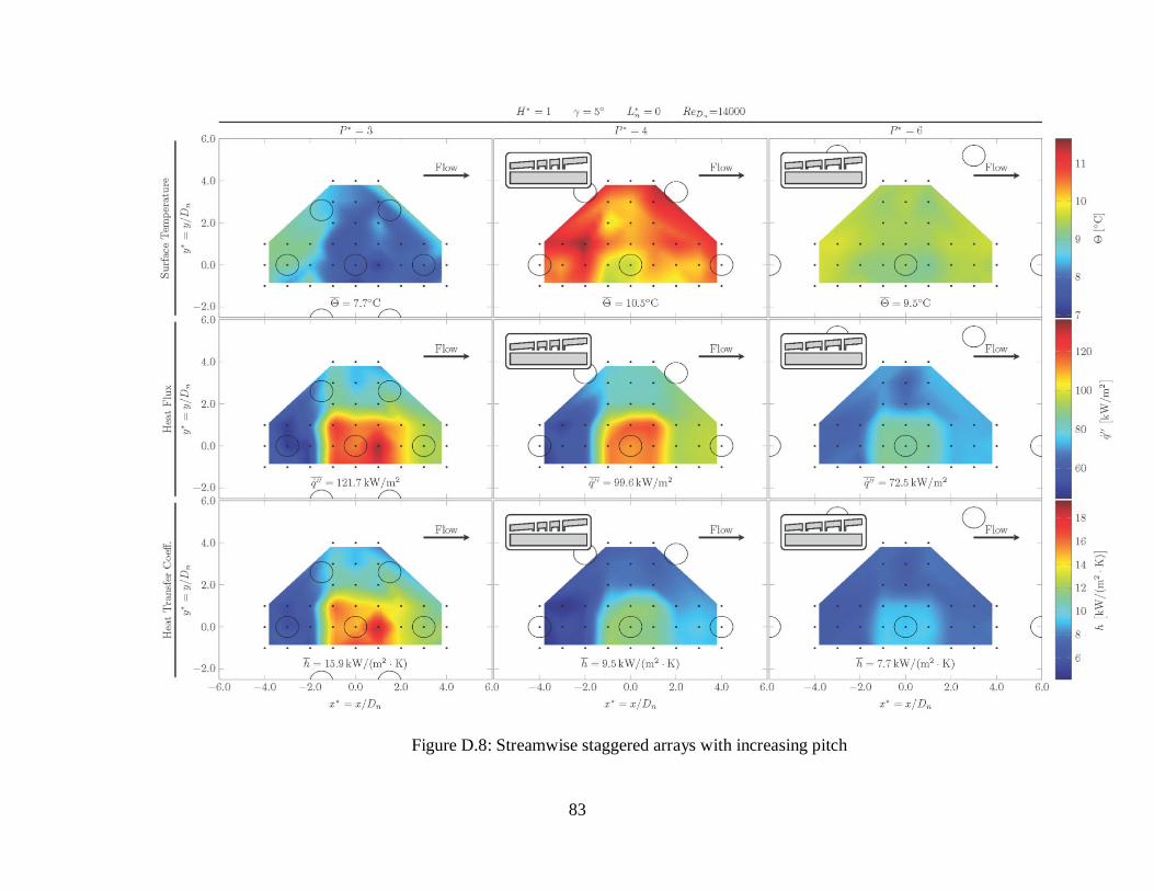
83

Figure D.8: Streamwise staggered arrays with increasing pitch

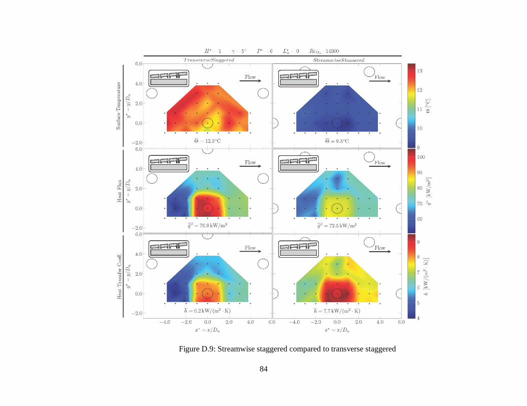
84

Figure D.9: Streamwise staggered compared to transverse staggered

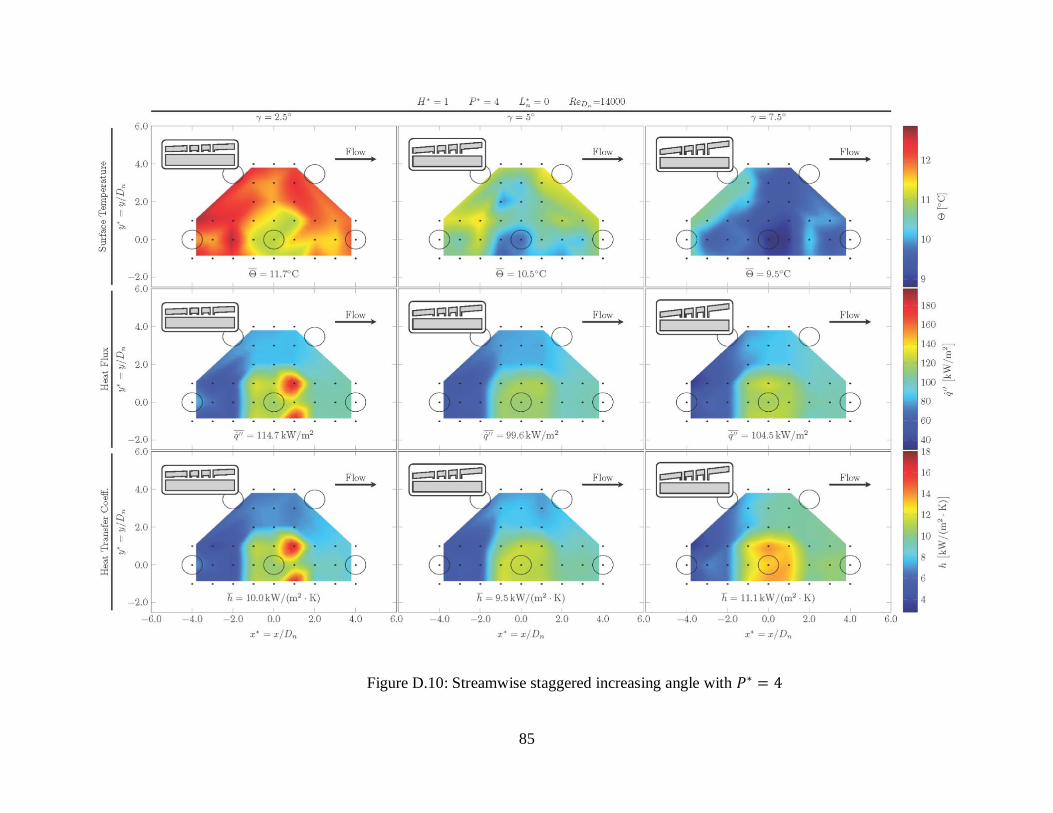
85

Figure D.10: Streamwise staggered increasing angle with 𝑃∗ = 4

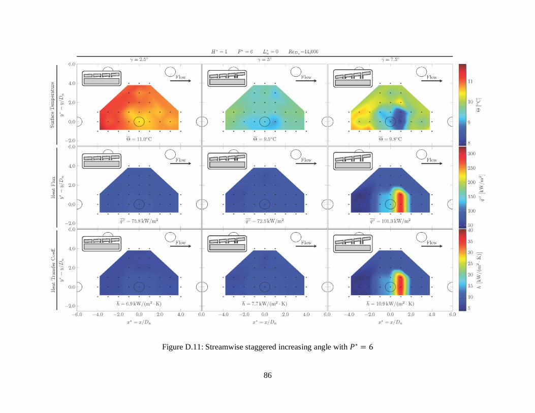
86

Figure D.11: Streamwise staggered increasing angle with 𝑃∗ = 6

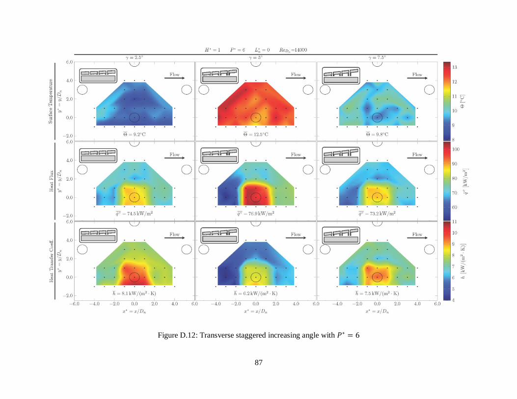
87

Figure D.12: Transverse staggered increasing angle with 𝑃∗ = 6

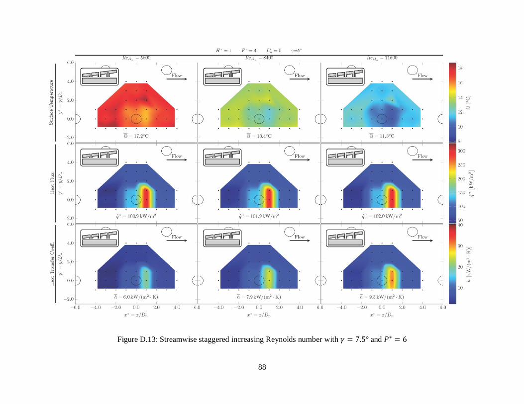
88

Figure D.13: Streamwise staggered increasing Reynolds number with 𝛾 = 7.5° and 𝑃∗ = 6