Embed Size (px)
Citation preview
SANDIA REPORTSAND2006-2540Unlimited ReleasePrinted May 2005
Staggered-Grid Finite-Difference AcousticModeling With the Time-DomainAtmospheric Acoustic Propagation Suite(TDAAPS)
Neill P. Symons, David F. Aldridge, Sandia National Laboratories; David H. Marlin, Sandra L.Collier U.S. Army Research Laboratory; D. Keith Wilson, U.S. Army Cold Regions Research& Engineering Lab.; Vladimir E. Ostashev, NOAA/Environmental Technology Laboratory
Prepared bySandia National LaboratoriesAlbuquerque, New Mexico 87185 and Livermore, California 94550
Sandia is a multiprogram laboratory operated by Sandia Corporation,a Lockheed Martin Company, for the United States Department of Energy’sNational Nuclear Security Administration under Contract DE-AC04-94-AL85000.
Approved for public release; further dissemination unlimited.
Issued by Sandia National Laboratories, operated for the United States Department ofEnergy by Sandia Corporation.
NOTICE: This report was prepared as an account of work sponsored by an agency ofthe United States Government. Neither the United States Government, nor any agencythereof, nor any of their employees, nor any of their contractors, subcontractors, or theiremployees, make any warranty, express or implied, or assume any legal liability or re-sponsibility for the accuracy, completeness, or usefulness of any information, appara-tus, product, or process disclosed, or represent that its use would not infringe privatelyowned rights. Reference herein to any specific commercial product, process, or serviceby trade name, trademark, manufacturer, or otherwise, does not necessarily constituteor imply its endorsement, recommendation, or favoring by the United States Govern-ment, any agency thereof, or any of their contractors or subcontractors. The views andopinions expressed herein do not necessarily state or reflect those of the United StatesGovernment, any agency thereof, or any of their contractors.
Printed in the United States of America. This report has been reproduced directly fromthe best available copy.
Available to DOE and DOE contractors fromU.S. Department of EnergyOffice of Scientific and Technical InformationP.O. Box 62Oak Ridge, TN 37831
Telephone: (865) 576-8401Facsimile: (865) 576-5728E-Mail: [email protected] ordering: http://www.doe.gov/bridge
Available to the public fromU.S. Department of CommerceNational Technical Information Service5285 Port Royal RdSpringfield, VA 22161
Telephone: (800) 553-6847Facsimile: (703) 605-6900E-Mail: [email protected] ordering: http://www.ntis.gov/ordering.htm
DEPA
RTMENT OF ENERGY
• • UN
ITED
STATES OF AM
ERIC
A
2
SAND2006-2540Unlimited ReleasePrinted May 2005
Staggered-Grid Finite-Difference AcousticModeling With the Time-Domain Atmospheric
Acoustic Propagation Suite (TDAAPS)
Neill P. Symons, David F. AldridgeSandia National Laboratories
Geophysics DepartmentAlbuquerque, NM 87185-0750
David H. Marlin, Sandra L. CollierU.S. Army Research Laboratory
D. Keith WilsonU.S. Army Cold Regions Research
Engineering Lab.
Vladimir E. OstashevNOAA/Environmental Technology Laboratory
3
Abstract
This document is intended to serve as a users guide for the time-domain atmosphericacoustic propagation suite (TDAAPS) program developed as part of the Department ofDefense High-Performance Modernization Office (HPCMP) Common High-PerformanceComputing Scalable Software Initiative (CHSSI). TDAAPS performs staggered-grid finite-difference modeling of the acoustic velocity-pressure system with the incorporation of spa-tially inhomogeneous winds. Wherever practical the control structure of the codes arewritten in C++ using an object oriented design. Sections of code where a large number ofcalculations are required are written in C or F77 in order to enable better compiler optimiza-tion of these sections. The TDAAPS program conforms to a UNIX style calling interface.Most of the actions of the codes are controlled by adding flags to the invoking commandline. This document presents a large number of examples and provides new users with thenecessary background to perform acoustic modeling with TDAAPS.
4
Acknowledgment
Funding for this work provided by the Department of Defense High-Performance Modern-ization Office (HPCMP) Common High-Performance Computing Scalable Software Initia-tive (CHSSI), project CEA-11. Thanks to the TDAAPS Alpha tester Micheal White fromERDC-CERL and Beta tester Rodney Whitaker from Los Alamos National Laboratory,who also provided many helpful comments on this document. This document was vastlyimproved after thoughtful and complete reviews by Mattew M. Haney and Sandford Bal-lard.
For code distribution, contact Dr. David Marlin ([email protected]).
5
Contents
Nomenclature 11
1 Introduction 13
1.1 Document Purpose . . . . . . . . . . . . . . . . . . . . . . . . . . . . . . . . . . . . . . . . . . . . . 13
1.2 Export Control . . . . . . . . . . . . . . . . . . . . . . . . . . . . . . . . . . . . . . . . . . . . . . . . 13
1.3 Design Choices . . . . . . . . . . . . . . . . . . . . . . . . . . . . . . . . . . . . . . . . . . . . . . . 14
1.3.1 C++ and C . . . . . . . . . . . . . . . . . . . . . . . . . . . . . . . . . . . . . . . . . . . . 14
1.3.2 NetCDF Files . . . . . . . . . . . . . . . . . . . . . . . . . . . . . . . . . . . . . . . . . . 14
1.3.3 Message Passing Protocol . . . . . . . . . . . . . . . . . . . . . . . . . . . . . . . . . 15
1.4 Concurrent Version System (CVS) . . . . . . . . . . . . . . . . . . . . . . . . . . . . . . . . 15
1.4.1 CVS Logging . . . . . . . . . . . . . . . . . . . . . . . . . . . . . . . . . . . . . . . . . . 17
1.5 Background . . . . . . . . . . . . . . . . . . . . . . . . . . . . . . . . . . . . . . . . . . . . . . . . . . 19
1.5.1 Moving-Media Acoustic Equations . . . . . . . . . . . . . . . . . . . . . . . . . 19
1.5.2 Finite-Difference . . . . . . . . . . . . . . . . . . . . . . . . . . . . . . . . . . . . . . . . 19
1.5.3 Parallel Implementation . . . . . . . . . . . . . . . . . . . . . . . . . . . . . . . . . . 20
2 Running the TDAAPS Algorithm 23
2.1 Basics of Running TDAAPS . . . . . . . . . . . . . . . . . . . . . . . . . . . . . . . . . . . . . . 23
2.1.1 Checkpoints . . . . . . . . . . . . . . . . . . . . . . . . . . . . . . . . . . . . . . . . . . . . 24
2.2 Dispersion and Stability . . . . . . . . . . . . . . . . . . . . . . . . . . . . . . . . . . . . . . . . . 24
6
2.3 Input Files . . . . . . . . . . . . . . . . . . . . . . . . . . . . . . . . . . . . . . . . . . . . . . . . . . . 25
2.3.1 Units . . . . . . . . . . . . . . . . . . . . . . . . . . . . . . . . . . . . . . . . . . . . . . . . . 25
2.3.2 Model Construction and MatlabTM . . . . . . . . . . . . . . . . . . . . . . . . . . 25
2.3.3 Text Input Files . . . . . . . . . . . . . . . . . . . . . . . . . . . . . . . . . . . . . . . . . 30
2.4 Output File Formats . . . . . . . . . . . . . . . . . . . . . . . . . . . . . . . . . . . . . . . . . . . . 30
2.5 Boundary Conditions . . . . . . . . . . . . . . . . . . . . . . . . . . . . . . . . . . . . . . . . . . . 32
2.5.1 Zwikker-Kosten (Mass-Resistance) Boundary Condition . . . . . . . . . 33
2.5.2 Rock Property (Irregular Surface) Boundary Condition . . . . . . . . . . 34
2.6 Quasi-Wavelets . . . . . . . . . . . . . . . . . . . . . . . . . . . . . . . . . . . . . . . . . . . . . . . 34
2.7 Usage and Definition of Flags . . . . . . . . . . . . . . . . . . . . . . . . . . . . . . . . . . . . 35
2.7.1 BNF Definition of TDAAPS call . . . . . . . . . . . . . . . . . . . . . . . . . . . . 37
2.7.2 Description of TDAAPS flags . . . . . . . . . . . . . . . . . . . . . . . . . . . . . . 37
3 Model Generation 41
3.1 Introduction . . . . . . . . . . . . . . . . . . . . . . . . . . . . . . . . . . . . . . . . . . . . . . . . . . 41
3.2 Model Building with MatlabTM . . . . . . . . . . . . . . . . . . . . . . . . . . . . . . . . . . . 42
3.3 Model Building with buildSgfdModel . . . . . . . . . . . . . . . . . . . . . . . . . . . . . . 48
3.3.1 Usage and Definition of Flags . . . . . . . . . . . . . . . . . . . . . . . . . . . . . . 48
3.3.2 BNF Definition of buildSgfdModel call . . . . . . . . . . . . . . . . . . . . . . 50
3.3.3 Description of buildSgfdModel flags . . . . . . . . . . . . . . . . . . . . . . . . . 50
4 Examples 51
4.1 Transmission Loss with Vertical Wind Gradient . . . . . . . . . . . . . . . . . . . . . . 51
4.2 Extinction and Coherence . . . . . . . . . . . . . . . . . . . . . . . . . . . . . . . . . . . . . . . 54
4.3 Alpha Test Scalability . . . . . . . . . . . . . . . . . . . . . . . . . . . . . . . . . . . . . . . . . . 59
4.4 Long Range Ultra-Low Frequency . . . . . . . . . . . . . . . . . . . . . . . . . . . . . . . . 62
7
Bibliography 71
Appendix
A TDAAPS Calling Flags Quick Reference 73
B Examples from the Beta Test 75
B.1 Hill Test . . . . . . . . . . . . . . . . . . . . . . . . . . . . . . . . . . . . . . . . . . . . . . . . . . . . . 75
B.2 Extinction and Coherence . . . . . . . . . . . . . . . . . . . . . . . . . . . . . . . . . . . . . . . 83
B.3 Zwikker-Kosten Partially Absorbing Boundary Condition . . . . . . . . . . . . . . 90
C Large Eddy Simulation (LES) Example 95
8
List of Figures
1.1 Double Time-Step Temporal Update . . . . . . . . . . . . . . . . . . . . . . . . . . . . . . . 21
1.2 Domain Decomposition . . . . . . . . . . . . . . . . . . . . . . . . . . . . . . . . . . . . . . . . . 22
2.1 Comparison of Slices from 3D and 1D Model . . . . . . . . . . . . . . . . . . . . . . . 29
2.2 QW Velocity Distributions . . . . . . . . . . . . . . . . . . . . . . . . . . . . . . . . . . . . . . . 36
3.1 Three Cross Sections Through the Hill Model . . . . . . . . . . . . . . . . . . . . . . . 49
4.1 100Hz mono-frequency source wavelet . . . . . . . . . . . . . . . . . . . . . . . . . . . . . 53
4.2 Trace output from Transmission Loss Example . . . . . . . . . . . . . . . . . . . . . . . 55
4.3 Trace output from Extinction and Coherence Example . . . . . . . . . . . . . . . . . 58
4.4 3D Wind Model for Low Frequency Example . . . . . . . . . . . . . . . . . . . . . . . . 67
4.5 Time-Slice from Low Frequency Example . . . . . . . . . . . . . . . . . . . . . . . . . . 68
9
List of Tables
1.1 CVS Revision Numbers: src/acoustic sgfd . . . . . . . . . . . . . . . . . . . . . . . . . . 16
1.2 CVS Revision Numbers: src/sgfd . . . . . . . . . . . . . . . . . . . . . . . . . . . . . . . . . 16
1.3 CVS Revision Numbers: src/utils . . . . . . . . . . . . . . . . . . . . . . . . . . . . . . . . . 17
10
Nomenclature
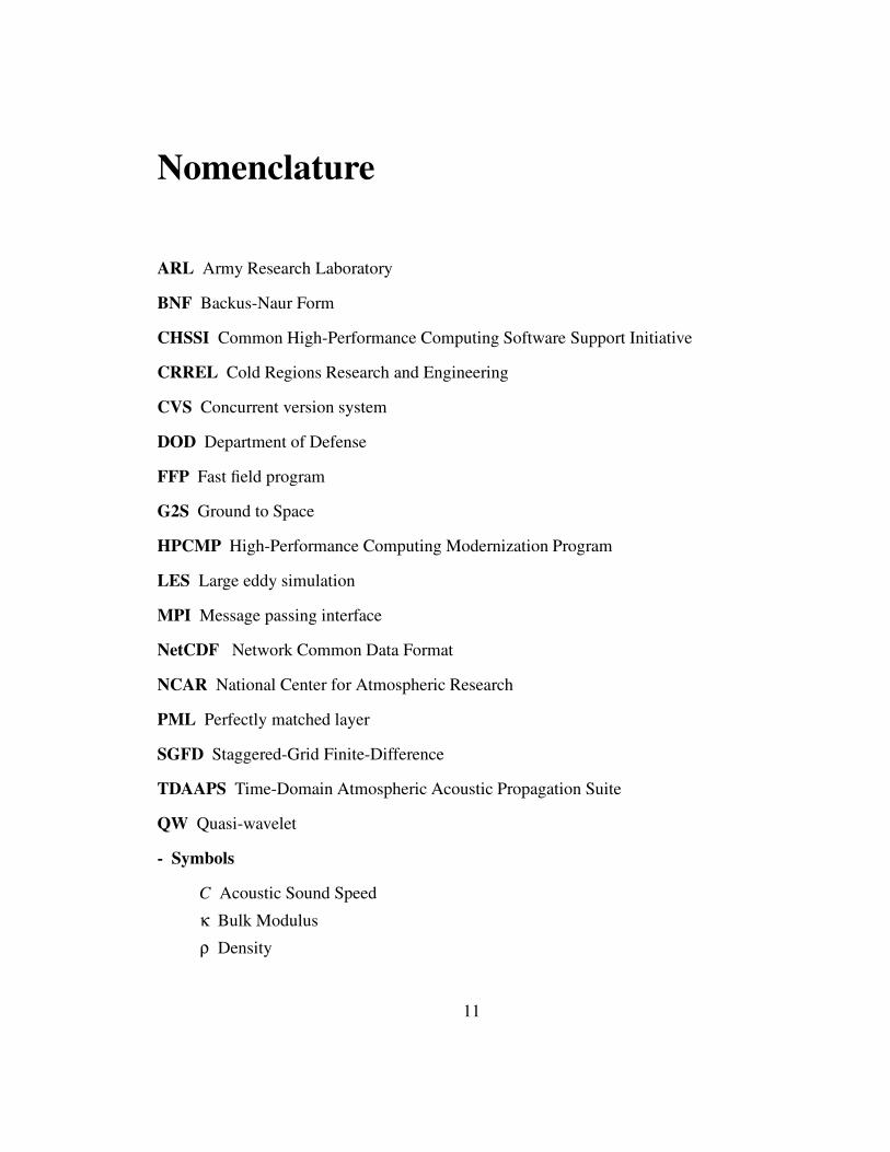
ARL Army Research Laboratory
BNF Backus-Naur Form
CHSSI Common High-Performance Computing Software Support Initiative
CRREL Cold Regions Research and Engineering
CVS Concurrent version system
DOD Department of Defense
FFP Fast field program
G2S Ground to Space
HPCMP High-Performance Computing Modernization Program
LES Large eddy simulation
MPI Message passing interface
NetCDF Network Common Data Format
NCAR National Center for Atmospheric Research
PML Perfectly matched layer
SGFD Staggered-Grid Finite-Difference
TDAAPS Time-Domain Atmospheric Acoustic Propagation Suite
QW Quasi-wavelet
- Symbols
C Acoustic Sound Speedκ Bulk Modulusρ Density
11

This page intentionally blank
12
Chapter 1
Introduction
1.1 Document Purpose
Staggered-grid finite-difference (SGFD) seismic modeling of the velocity-stress system ofelastodynamics has been described by a number of authors. Some of the most impor-tant papers include Virieux (1986); Bayliss et al. (1986); Levander (1988); Graves (1996).However, modeling of the similar acoustic, velocity-pressure equations with the incorpo-ration of spatially inhomogeneous wind is a fairly recent development. This document isintended to serve as a users guide for the TDAAPS program which has been developedas a joint project of the Army Research Laboratory (ARL), Sandia National Laboratories(SNL), U. S. Army Engineer Research and Development Center Cold Regions Researchand Engineering Laboratory (ERDC-CRREL), National Oceanic and Atmospheric Admin-istration Environmental Technologies Laboratory (NOAA-ETL), and the National Centerfor Atmospheric Research (NCAR). Funding for the his project has been provided by theDepartment of Defense Common High-Performance Software Support Initiative (CHSSI).
1.2 Export Control
The source and executable code for TDAAPS are export controlled at the present time.Some of the code is shared with other staggered-grid finite-difference applications devel-oped by Neill Symons at SNL and is not export controlled. All export controlled filescontain the following warning (usually in a C style comment) at the top:
WARNING - This document contains technical data whose export isrestricted by the Export Administration Act of 1979, as amended, (50App. U.S.C. 2401 et seq). Violations of these export laws are subjectto severe civil and criminal penalties.
The output of the code, operational manuals (such as this document), and mathematical
13
descriptions are not export controlled.
1.3 Design Choices
1.3.1 C++ and C
Wherever practical, the control structure of the codes are written in C++ using an objectoriented design. This makes for clear, well-documented code that can easily be modifiedto include more features. For instance, the model for static acoustics consists of only twomodel parameters: c and ρ. When modeling moving-media, a subclass of this main modelis used containing the extra model parameters needed to specify the wind speeds.
Object oriented C++ classes are used to define: models, collections of dependent vari-ables, networks of receivers and individual receiver types, networks of sources and individ-ual source types, and the variety of possible types of boundary conditions.
Sections of code where a large number of calculations are required are written in C orF77 in order to enable better compiler optimization of these sections. Examples are thevelocity and pressure updating subroutines that access every interior model point for everytime-step. These subroutines are linked into the C++ control structure using the
#if defined(__cplusplus)extern "C" #endif
...
...
...#if defined(__cplusplus)#endif
directive set.
1.3.2 NetCDF Files
A major feature of TDAAPS is the extensive use of NetCDF (Rew et al., 1997) for inputand output files. NetCDF files have five advantages over other possible formats for use inthis context. (1) These files are machine portable. As long as the files are accessed usingthe provided interface, any conversion necessitated by different numerical storage schemes(i.e. big endian to little endian) is performed transparently to the user. (2) NetCDF filesare small and fast to access, the files are only slightly larger than a raw binary format,and moreover, the time to read or write NetCDF format is only slightly slower that fora raw binary file. This was not true for earlier versions of the interface. (3) The formatis self documenting and unlike binary files, NetCDF uses named variables which provide
14
some information about what is contained within the file. The values of variables can beexamined by using the program ncdump, which is part of the NetCDF package. (4) It iseasy to add or delete additional information as required. Since the file is accessed via thenamed NetCDF variables, adding additional fields to the file does not require updating allprograms that use that file format. (5) NetCDF files are easily read into and written fromMatlabTM using the Denham (2000) MexCDF package. This allows for easy visualizationof the model results and can be invaluable for interpretation of the modeling results froma complex atmospheric model. Use of MatlabTM for writing model files gives the user aneasy way to build complex 3D atmospheric models to be used in TDAAPS.
1.3.3 Message Passing Protocol
Message passing for TDAAPS is accomplished using either the Message Passing Interface(MPI) or the Parallel Virtual Machine (PVM) interface (Geist et al., 1996). The choiceis determined by the inclusion of one of two possible object files during the link phaseof compiling the executable. The MPI interface is the standard and is the only availablemethod on many platforms including many of the DOD HPC platforms. The PVM interfaceis widely available on Linux Beowulf platforms and has some advantages for applicationdevelopment; there is a better suite of debugging tools available. In order the allow theuse of either of these two protocols, all message passing calls within the application aremade through a set of wrapper subroutines that have been implemented in different files,one using MPI and the other with PVM.
1.4 Concurrent Version System (CVS)
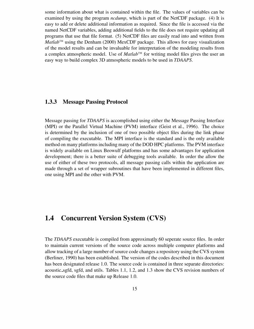
The TDAAPS executable is compiled from approximatly 60 seperate source files. In orderto maintain current versions of the source code across multiple computer platforms andallow tracking of a large number of source code changes a repository using the CVS system(Berliner, 1990) has been established. The version of the codes described in this documenthas been designated release 1.0. The source code is contained in three separate directories:acoustic sgfd, sgfd, and utils. Tables 1.1, 1.2, and 1.3 show the CVS revision numbers ofthe source code files that make up Release 1.0.
15
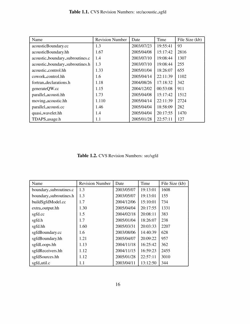
Table 1.1. CVS Revision Numbers: src/acoustic sgfd
Name Revision Number Date Time File Size (kb)acousticBoundary.cc 1.3 2003/07/23 19:55:41 93acousticBoundary.hh 1.67 2005/04/08 15:17:42 2816acoustic boundary subroutines.c 1.4 2003/07/10 19:08:44 1307acoustic boundary subroutines.h 1.3 2003/07/10 19:08:44 255acoustic control.hh 1.33 2005/01/04 18:26:07 655cowork control.hh 1.6 2005/04/14 22:11:39 1102fortran declarations.h 1.18 2004/08/26 17:18:32 342generateQW.cc 1.15 2004/12/02 00:53:08 911parallel acousti.hh 1.73 2005/04/08 15:17:42 1512moving acoustic.hh 1.110 2005/04/14 22:11:39 2724parallel acousti.cc 1.46 2005/04/04 18:58:09 282quasi wavelet.hh 1.4 2005/04/04 20:17:55 1470TDAPS usage.h 1.1 2005/01/28 22:57:11 127
Table 1.2. CVS Revision Numbers: src/sgfd
Name Revision Number Date Time File Size (kb)boundary subroutines.c 1.3 2003/05/07 19:13:01 1608boundary subroutines.h 1.3 2003/05/07 19:13:01 155buildSgfdModel.cc 1.7 2004/12/06 15:10:01 734extra output.hh 1.30 2005/04/04 20:17:55 1331sgfd.cc 1.5 2004/02/18 20:08:11 383sgfd.h 1.7 2005/01/04 18:26:07 238sgfd.hh 1.60 2005/03/31 20:03:33 2207sgfdBoundary.cc 1.6 2003/08/06 14:40:39 628sgfdBoundary.hh 1.21 2005/04/07 20:09:22 957sgfdLoops.hh 1.13 2004/11/18 16:25:42 362sgfdReceivers.hh 1.12 2004/11/15 16:59:23 2455sgfdSources.hh 1.12 2005/01/28 22:57:11 3010sgfd util.c 1.1 2003/04/11 13:12:50 344
16
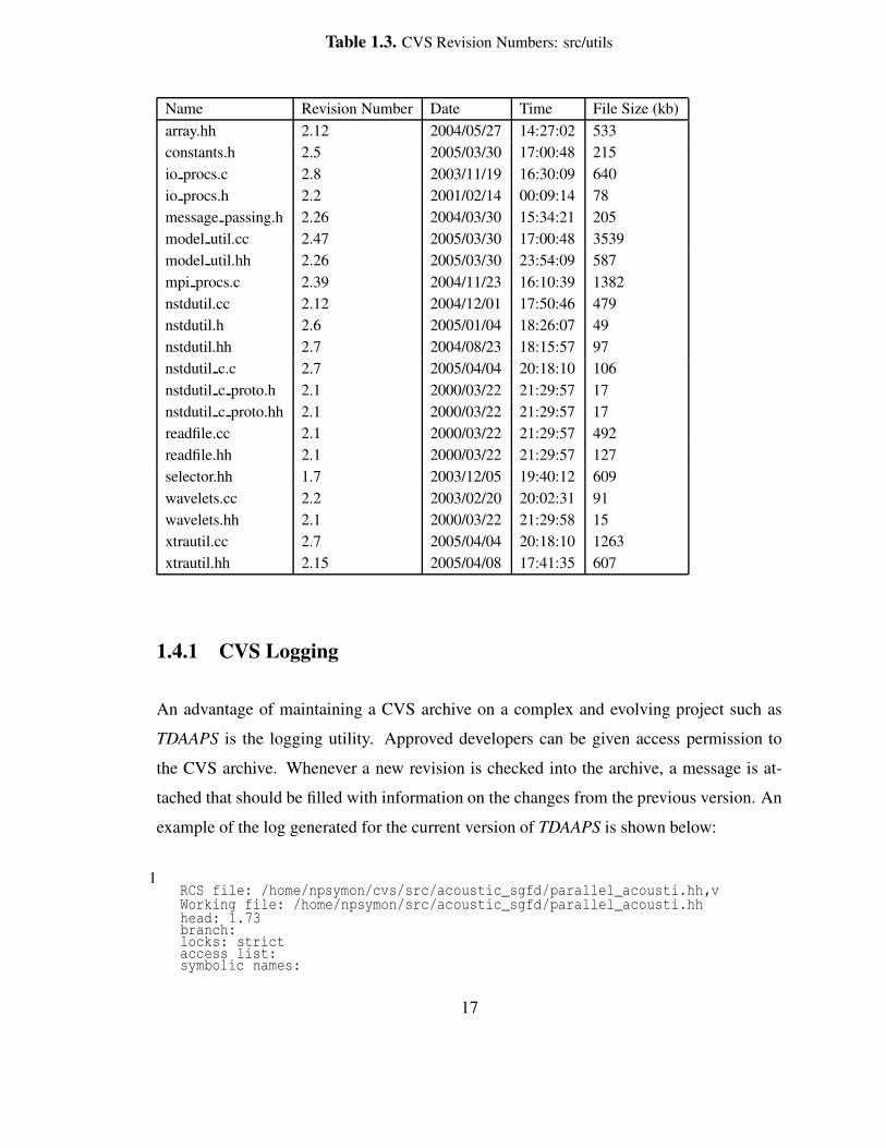
Table 1.3. CVS Revision Numbers: src/utils
Name Revision Number Date Time File Size (kb)array.hh 2.12 2004/05/27 14:27:02 533constants.h 2.5 2005/03/30 17:00:48 215io procs.c 2.8 2003/11/19 16:30:09 640io procs.h 2.2 2001/02/14 00:09:14 78message passing.h 2.26 2004/03/30 15:34:21 205model util.cc 2.47 2005/03/30 17:00:48 3539model util.hh 2.26 2005/03/30 23:54:09 587mpi procs.c 2.39 2004/11/23 16:10:39 1382nstdutil.cc 2.12 2004/12/01 17:50:46 479nstdutil.h 2.6 2005/01/04 18:26:07 49nstdutil.hh 2.7 2004/08/23 18:15:57 97nstdutil c.c 2.7 2005/04/04 20:18:10 106nstdutil c proto.h 2.1 2000/03/22 21:29:57 17nstdutil c proto.hh 2.1 2000/03/22 21:29:57 17readfile.cc 2.1 2000/03/22 21:29:57 492readfile.hh 2.1 2000/03/22 21:29:57 127selector.hh 1.7 2003/12/05 19:40:12 609wavelets.cc 2.2 2003/02/20 20:02:31 91wavelets.hh 2.1 2000/03/22 21:29:58 15xtrautil.cc 2.7 2005/04/04 20:18:10 1263xtrautil.hh 2.15 2005/04/08 17:41:35 607
1.4.1 CVS Logging
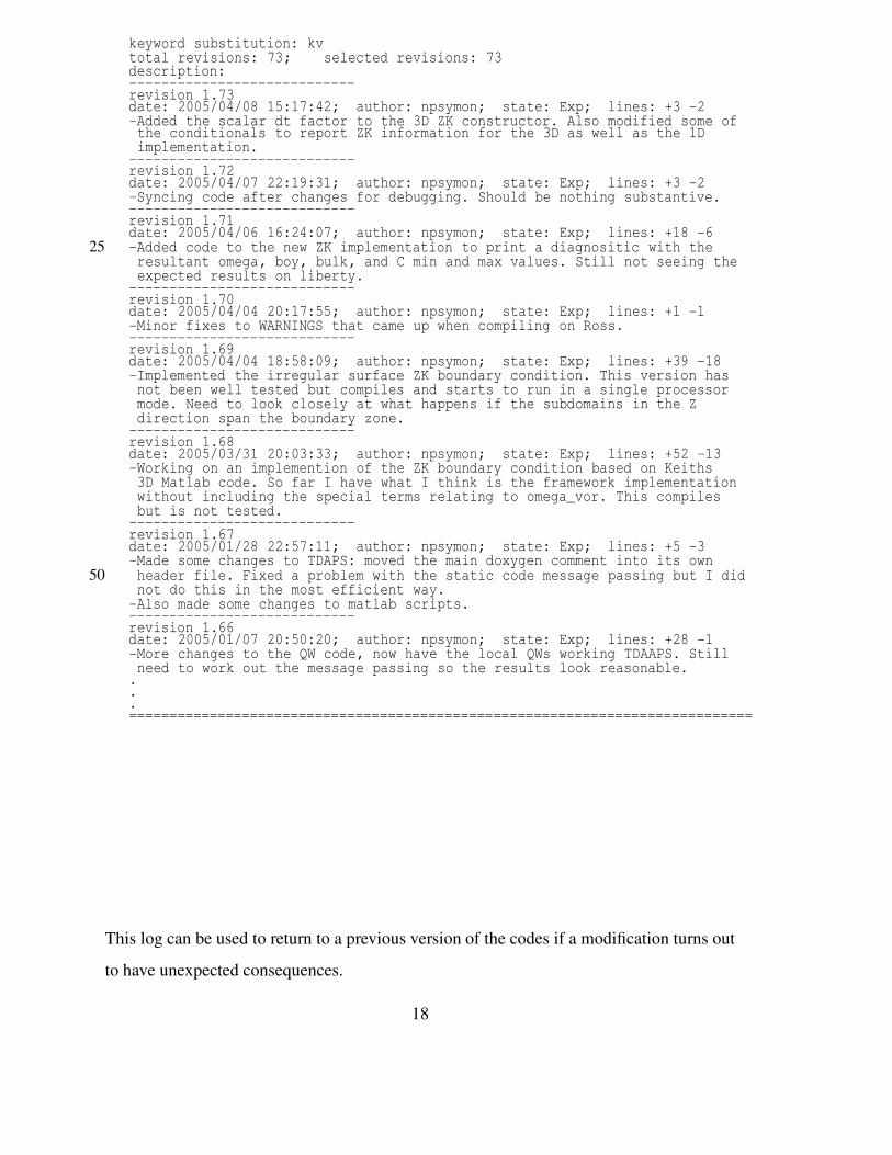
An advantage of maintaining a CVS archive on a complex and evolving project such asTDAAPS is the logging utility. Approved developers can be given access permission tothe CVS archive. Whenever a new revision is checked into the archive, a message is at-tached that should be filled with information on the changes from the previous version. Anexample of the log generated for the current version of TDAAPS is shown below:
1RCS file: /home/npsymon/cvs/src/acoustic_sgfd/parallel_acousti.hh,vWorking file: /home/npsymon/src/acoustic_sgfd/parallel_acousti.hhhead: 1.73branch:locks: strictaccess list:symbolic names:
17
keyword substitution: kvtotal revisions: 73; selected revisions: 73description:----------------------------revision 1.73date: 2005/04/08 15:17:42; author: npsymon; state: Exp; lines: +3 -2-Added the scalar dt factor to the 3D ZK constructor. Also modified some ofthe conditionals to report ZK information for the 3D as well as the 1Dimplementation.
----------------------------revision 1.72date: 2005/04/07 22:19:31; author: npsymon; state: Exp; lines: +3 -2-Syncing code after changes for debugging. Should be nothing substantive.----------------------------revision 1.71date: 2005/04/06 16:24:07; author: npsymon; state: Exp; lines: +18 -6
25 -Added code to the new ZK implementation to print a diagnositic with theresultant omega, boy, bulk, and C min and max values. Still not seeing theexpected results on liberty.
----------------------------revision 1.70date: 2005/04/04 20:17:55; author: npsymon; state: Exp; lines: +1 -1-Minor fixes to WARNINGS that came up when compiling on Ross.----------------------------revision 1.69date: 2005/04/04 18:58:09; author: npsymon; state: Exp; lines: +39 -18-Implemented the irregular surface ZK boundary condition. This version hasnot been well tested but compiles and starts to run in a single processormode. Need to look closely at what happens if the subdomains in the Zdirection span the boundary zone.
----------------------------revision 1.68date: 2005/03/31 20:03:33; author: npsymon; state: Exp; lines: +52 -13-Working on an implemention of the ZK boundary condition based on Keiths3D Matlab code. So far I have what I think is the framework implementationwithout including the special terms relating to omega_vor. This compilesbut is not tested.
----------------------------revision 1.67date: 2005/01/28 22:57:11; author: npsymon; state: Exp; lines: +5 -3-Made some changes to TDAPS: moved the main doxygen comment into its own
50 header file. Fixed a problem with the static code message passing but I didnot do this in the most efficient way.
-Also made some changes to matlab scripts.----------------------------revision 1.66date: 2005/01/07 20:50:20; author: npsymon; state: Exp; lines: +28 -1-More changes to the QW code, now have the local QWs working TDAAPS. Stillneed to work out the message passing so the results look reasonable.
.
.
.=============================================================================
This log can be used to return to a previous version of the codes if a modification turns out
to have unexpected consequences.
18
1.5 Background
1.5.1 Moving-Media Acoustic Equations
The algorithm discussed in this document is based on the non-dimensionalized velocity-
pressure equations of linear elastodynamics, a set of four, coupled, first-order partial dif-
ferential equations (Ostashev et al., 2005):
∂w(x, t)∂t +(v ·∇)w+(w ·∇)v+b∇p = bf (1.1)
and∂p(x, t)
∂t +v ·∇p+κ∇ ·w =∂e(x, t)
∂t (1.2)
where w is the particle velocity, p is the pressure, and the ambient wind velocity is v. κ is
the bulk modulus, and b = 1ρ is the mass buoyancy. The inhomogeneous terms correspond
to the sources: f are force sources and e are energy density scalars corresponding to moment
sources.
1.5.2 Finite-Difference
An explicit, time-domain, finite-difference (FD) scheme is used to solve these four equa-
tions for the three components of the particle velocity vector and the pressure (e.g., Virieux,
1986; Bayliss et al., 1986; Levander, 1988; Graves, 1996). Centered spatial and temporal
FD operators possess 4th-order and 2nd-order accuracy in the discretization intervals, re-
spectively. The four independent variables are stored on uniform, but staggered, spatial and
temporal grids. The grid is chosen such that the primary (corner) nodes contain the six at-
mospheric model parameters and the pressure. The velocities are stored on the edges of the
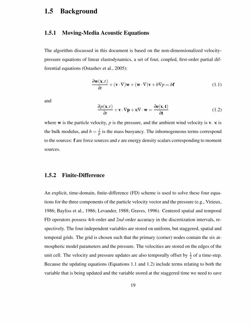
unit cell. The velocity and pressure updates are also temporally offset by 12 of a time-step.
Because the updating equations (Equations 1.1 and 1.2) include terms relating to both the
variable that is being updated and the variable stored at the staggered time we need to save
19
two time steps to keep all of the temporal updating equations centered in time. Figure 1.1
shows a pictorial version of the update stencils for one spatial dimension and time.
This computational algorithm is a direct numerical implementation of the governing
partial differential equations of linear acoustic propagation. No theoretical approxima-
tions, such as far-field distances, high frequencies, weak scattering, or one-way wave prop-
agation, are adopted. Hence, the algorithm generates all arrival types (direct, reflections,
refractions, multiples, diffractions, head waves, etc.) with fidelity, provided spatial and
temporal gridding intervals are chosen appropriately.
1.5.3 Parallel Implementation
In order to treat large-scale atmospheric model and datasets within reasonable execution
times, TDAAPS implements a parallel computational version of the basic algorithm (Symons
et al., 2003; Symons and Aldridge, 2000). This parallel implementation utilizes spatial do-
main decomposition: different portions of the 3D gridded atmospheric model are allocated
to different processors so that calculations within each such sub-domain take place syn-
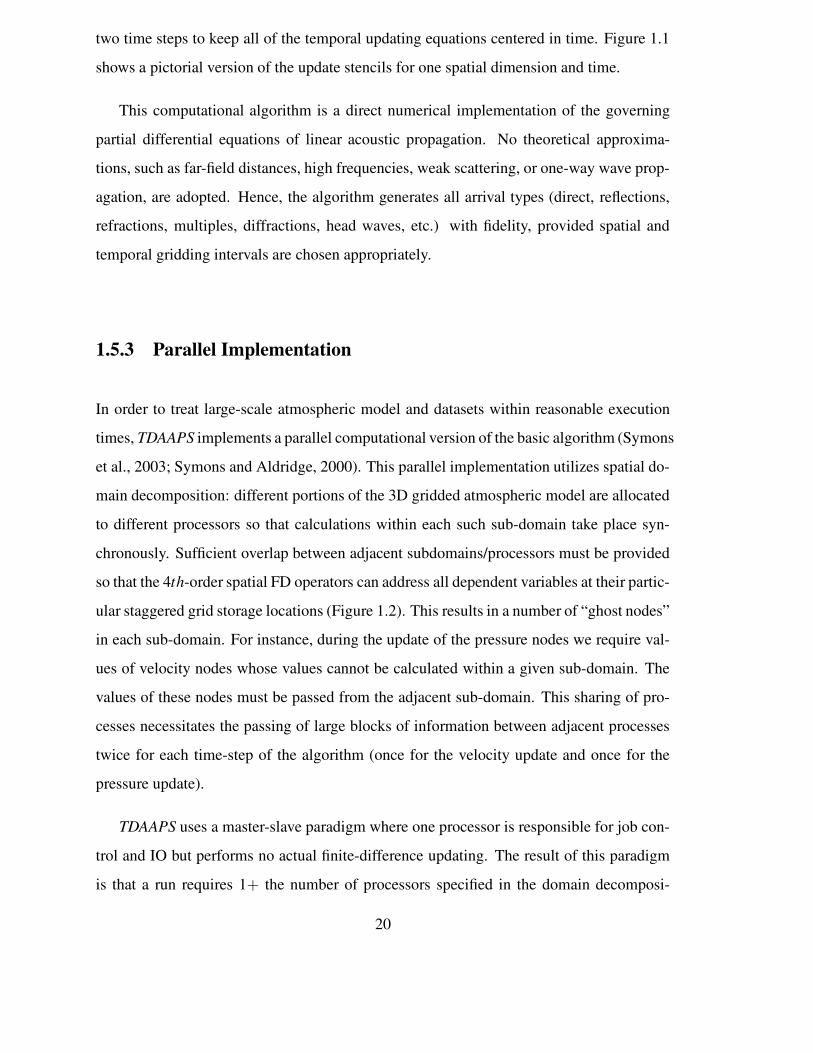
chronously. Sufficient overlap between adjacent subdomains/processors must be provided
so that the 4th-order spatial FD operators can address all dependent variables at their partic-
ular staggered grid storage locations (Figure 1.2). This results in a number of “ghost nodes”
in each sub-domain. For instance, during the update of the pressure nodes we require val-
ues of velocity nodes whose values cannot be calculated within a given sub-domain. The
values of these nodes must be passed from the adjacent sub-domain. This sharing of pro-
cesses necessitates the passing of large blocks of information between adjacent processes
twice for each time-step of the algorithm (once for the velocity update and once for the
pressure update).
TDAAPS uses a master-slave paradigm where one processor is responsible for job con-
trol and IO but performs no actual finite-difference updating. The result of this paradigm
is that a run requires 1+ the number of processors specified in the domain decomposi-
20
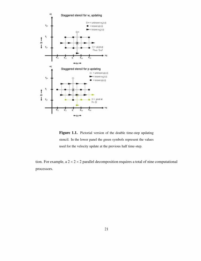
Figure 1.1. Pictorial version of the double time-step updating
stencil. In the lower panel the green symbols represent the values
used for the velocity update at the previous half time-step.
tion. For example, a 2×2×2 parallel decomposition requires a total of nine computational
processors.
21
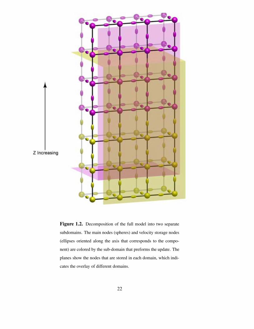
Figure 1.2. Decomposition of the full model into two separate
subdomains. The main nodes (spheres) and velocity storage nodes
(ellipses oriented along the axis that corresponds to the compo-
nent) are colored by the sub-domain that preforms the update. The
planes show the nodes that are stored in each domain, which indi-
cates the overlay of different domains.
22
Chapter 2
Running the TDAAPS Algorithm
2.1 Basics of Running TDAAPS
The TDAAPS program conforms to a UNIX style calling interface. Most of the actionsof the codes are controlled by adding flags (beginning with “-”) to the invoking commandline. For instance, to define 2×2×2 parallel decomposition in TDAAPS, the call takes theform:
> mpirun -np 9 \$\TDAAPS_PATH\/TDAAPS -p 2 2 2
where $TDAAPS PATHis an environment variable defined as the full path to the exe-
cutable. See Section 1.5.3 for an explanation of why nine processors are required for this
run. In order to reduce the length of the command line, several arguments can be combined
into a file which is specified on the command line. Recursion of argument files is allowed
(e.g., a command file may contain the name of another file, etc.); however, there is no check
for infinite recursion.
23
2.1.1 Checkpoints
Since large runs of TDAAPS may take a (very) long time on a large number of processors,
the algorithm incorporates a checkpoint utility. If this option is activated (using the -C flag),
TDAAPS will write the current state into a number of files in the user specified directory.
For large runs this will take significant space, so care must be applied to make sure that
the directory exists on a disk with enough free space. The directory must be fully qualified
since the individual processes will be writing several separate files. If TDAAPS is called
with the checkpoint option, it first checks for an existing checkpoint in the specified direc-
tory. If a checkpoint exists and the model and call are identical, then the run will commence
using the stored information from the iteration where the checkpoint was written.
2.2 Dispersion and Stability
A critical factor for any numerical simulation is that the solution be stable. Finite-difference
algorithms (such as TDAAPS) must also satisfy a dispersion criteria if the solution is to
provide meaningful results. A common rule of thumb for 4th order spatial algorithms (such
as this one) is the requirement of 5 nodes per wavelength of the source. This rule is often
stated (or refuted) without further elaboration. In reality, any source-time function that the
user chooses to input will contain a range of frequencies. To get good results, it is the
highest far-field propagating frequency that must fit the 5 nodes per wavelength criteria.
For high wind speeds it is also important to account for the reduced apparent velocity (and
therefore wavelength) of a signal that propagates upwind. The stability limit is related to
the Courant (CFL) number (∼ 2vmax∆t/h). For the moving-media acoustic problem this
number must be less than 1.
For a given modeling situation, a typical sequence of calculations to determine the
model parameters might be: (1) determine the minimum apparent velocity (c-v); (2) deter-
mine the highest frequency energy that will be propagating from the source (this is usually
taken as the 1% level of the amplitude spectrum of the source-time function); (3) using
24
these values, determine a reasonable grid spacing; (4) use the grid spacing and the highest
apparent velocity in the model determine a ∆t that yields a CFL less than 1. Note that
doubling the highest frequency typically requires halving the grid spacing which further
implies that the time step must be cut in half. This means that the work required increases
by 24 for every doubling of the source frequency.
2.3 Input Files
2.3.1 Units
TDAAPS does not enforce any specific set of units for the input files. However, the units
used on the input files will determine the units of the output files. In use, we have commonly
found it convenient to use MKS units for the input files; then pressure traces will have units
of Pa and velocity traces will have units of m/s. For large scale (i.e. hundreds of km)
simulations is can be more convenient to define the axis in km instead of m. This requires
that the acoustic velocity be specified in km/s, the result is that output velocity traces will
also be in km/s and pressure output will have units of N/km2. Internally the TDAAPS algo-
rithm works with non-dimensionalized values to provide the maximum possible numerical
accuracy with single precision values. The default non-dimensionalizing scalars are appro-
priate for MKS units, and “normal” atmospheric properties up to distances of several km.
Much longer or shorter propagation distances and different units might achieve increased
numerical accuracy by modification of the these values but this has not been investigated.
2.3.2 Model Construction and MatlabTM
All of the following discussion assumes that the Denham (2000) MexCDF package has
been correctly installed on the user’s system. This package allows the reading and writing
of NetCDF files from within MatlabTM using standard MatlabTM object oriented program-
25
ming constructs. The primary input to any run of TDAAPS is a model file. Chapter 3
contains descriptions of a variety of methods to create simple model files. The model is
always a NetCDF file with a certain minimum number of dimensions and variables. The
file must define:
1. The dimensions NX, NY, NZ, and NT.
2. The starting points for each of the vectors defining the axes in a variable called
minima.
3. The increments for each of the vectors defining the axes in a variable called increments.
4. A specification of the acoustic velocity (c) for all the points of the 3D grid in variable
named either C or Vp.
5. The density (ρ) for all the points of the 3D grid in a variable named Rho.
The most obvious (but also the most disk intensive) way to define c and ρ is to define two3D variables in the model with point by point values. To utilize this method of modeldefinition two 3D variables named C and Rho are defined in the model and the desiredvalues are assigned to them. The following MatlabTM script (simple model.m) builds aminimum input model:
1 %% Define the axes vectors and sizes.dx=1;dt=0.001;x=[-100:dx:100];y=[-50:dx:50];z=[-2:dx:75];t=[0:dt:0.5];
10 NX=length(x);NY=length(y);NZ=length(z);NT=length(t);%% Open the model for writing.out=netcdf(’simple_model.cdf’,’clobber’);%% Define the four reqired dimensions.out(’NX’)=NX;
20 out(’NY’)=NY;out(’NZ’)=NZ;out(’NT’)=NT;%% Define and fill the increment variables; note, this requires another
26
% dimension that is not used by TDAAPS.out(’numCoord’)=4; %This is used internally so we can define a vector of% starting values and increments.out’minima’=ncfloat(’numCoord’);out’minima’(:)=[x(1) y(1) z(1) t(1)];
30 out’increments’=ncfloat(’numCoord’);out’increments’(:)=[dx dx dx dt];%% Define and fill the values that define the model.out’C’=ncfloat(’NZ’,’NY’,’NX’);out’C’(:,:,:)=342*ones([NZ NY NX]); %Sound speed 342 m/sout’Rho’=ncfloat(’NZ’,’NY’,’NX’);out’Rho’(:,:,:)=1.2*ones([NZ NY NX]); %Density 1.2 kg/mˆ3%% And close the file
40 close(out);
Since the atmospheric model is often 1D (with 3D features added with quasi-wavelets orother complex wind conditions) the code will also read a model file which defines the modelvalues with 1D arrays of the same length as the z-axis. These variables have oneDModel
pre-pended to the analogous 3D names. The following MatlabTM script (simple model 1D.m)builds a model which is identical to the 3D model (when read by TDAAPS):
1 %% Define the axes vectors and sizes.dx=1;dt=0.001;x=[-100:dx:100];y=[-50:dx:50];z=[-2:dx:75];t=[0:dt:0.5];
10 NX=length(x);NY=length(y);NZ=length(z);NT=length(t);%% Open the model for writing.out=netcdf(’simple_model_1D.cdf’,’clobber’);%% Define the four reqired dimensions.out(’NX’)=NX;
20 out(’NY’)=NY;out(’NZ’)=NZ;out(’NT’)=NT;%% Define and fill the increment variables; note, this requires another% dimension that is not used by TDAPS.out(’numCoord’)=4; %This is used internally so we can define a vector of% starting values and increments.out’minima’=ncfloat(’numCoord’);out’minima’(:)=[x(1) y(1) z(1) t(1)];
30 out’increments’=ncfloat(’numCoord’);out’increments’(:)=[dx dx dx dt];%% Define and fill the values that define the model.out’oneDModelVp’=ncfloat(’NZ’);out’oneDModelVp’(:,:,:)=342*ones([1 NZ]);out’oneDModelRho’=ncfloat(’NZ’);out’oneDModelRho’(:,:,:)=1.2*ones([1 NZ]);%% And close the file
40 close(out);
27
However, the 1D model occupies 916bytes while the 3D model takes 12Mb on a Linux
workstation. As will be discussed in more detail in Section 2.4, TDAAPS creates two
primary types of output files. Trace files contain the complete time history at a given point,
and slice files contain a (set of) snapshot(s) of the entire space of the model along a user
defined plane at a single time.
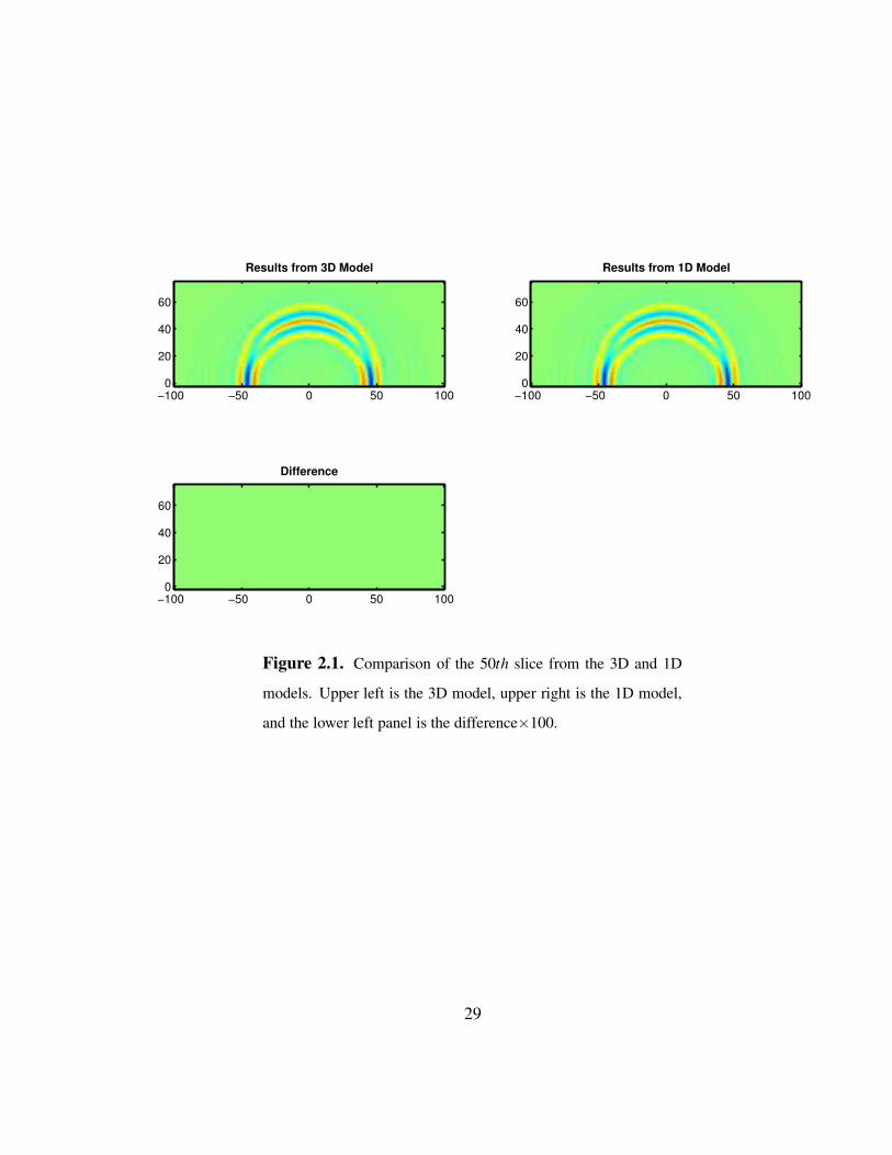
We have verified that runs of TDAAPS with the 3D and 1D models yield identical resultsby performing runs with both and examining the slice output with MatlabTM:
1 %% Open the slice files that we are comparing.in3D=netcdf(’slice.3D.cdf’);in1D=netcdf(’slice.1D.cdf’);%% Get some vectors for the axes.x=in3D’x’(:);z=in3D’z’(:);%% Plot the 40th slice from each file in the upper left and right panels.
10 sliceIndex=40;subplot(2,2,1);imagesc(x,z,squeeze(in3D’xzPressure’(sliceIndex,:,:)));axis image;caxis([-1e-3 1e-3]);set(gca,’FontSize’,15,’LineWidth’,2,’Box’,’on’,’YDir’,’normal’);title(’Results from 3D Model’,’FontWeight’,’Bold’);subplot(2,2,2);imagesc(x,z,squeeze(in1D’xzPressure’(sliceIndex,:,:)));
20 axis image;caxis([-1e-3 1e-3]);set(gca,’FontSize’,15,’LineWidth’,2,’Box’,’on’,’YDir’,’normal’);title(’Results from 1D Model’,’FontWeight’,’Bold’);%% And plot the difference x100 in the lower left panel.subplot(2,2,3);imagesc(x,z,...
squeeze(in3D’xzPressure’(sliceIndex,:,:))-...squeeze(in1D’xzPressure’(sliceIndex,:,:)));
30 axis image;caxis([-1e-5 1e-5]);set(gca,’FontSize’,15,’LineWidth’,2,’Box’,’on’,’YDir’,’normal’);title(’Difference’,’FontWeight’,’Bold’);
This script gives the result shown in Figure 2.1.
Spatially variable 3D wind fields can also be input in a similar format. For the the
wind model files the 3D variables are WindVx, WindVy, and WindVz. As with the atmo-
spheric model definitions the user can substitute oneDModelWindVx, oneDModelWindVy,
and oneDModelWindVz if desired to decrease the file size. Note that all the runs performed
for the Alpha and Beta tests build a wind profile using the limited menu of pre-defined
28
Results from 3D Model
−100 −50 0 50 1000
20
40
60
Results from 1D Model
−100 −50 0 50 1000
20
40
60
Difference
−100 −50 0 50 1000
20
40
60
Figure 2.1. Comparison of the 50th slice from the 3D and 1D
models. Upper left is the 3D model, upper right is the 1D model,
and the lower left panel is the difference×100.
29
types on the TDAAPS command line.
2.3.3 Text Input Files
There are a few types of text input files. Two examples are source-time functions, which
are input as two columns of time and value, and receiver locations which can be read as
either three column (x, y, z) or four column (x, y, z, sensitivity).
2.4 Output File Formats
There are two major types of output files produced by TDAAPS, trace files and slice files.Chapter 4 contains examples of using MatlabTM to plot results directly from these files.Both file types contain dimensions that define the model size (NX, NY, NZ, and NT). Thereare corresponding variables that define the axes (x, y, z, and time). In the trace file, thereare also dimensions that define the number of receivers (numReceivers). There are then aset of variables that show: the receiver type, sensitivity, location, orientation, if the valueshave been integrated or differentiated, and a numReceivers ×NT matrix of results. Forconvenience, if the output is to be compared to the source waveform, this file also containsa description of the sources used during the run (either defined as part of the model or onthe TDAAPS command line). The following is the output from running the command
> ncdump -h trace.cdf
on the trace file created from the simplest possible run of TDAAPS. The ncdump command
is part of the NetCDF package and can be used to view the entire contents (or just the
header with the -h flag) of a NetCDF file.
1 netcdf trace dimensions:
numCoord = 4 ;numSpatialCoord = 3 ;NX = 50 ;NY = 25 ;NZ = 50 ;
30
NT = 501 ;numReceivers = 33 ;
10 numMSources = 1 ;variables:
float minima(numCoord) ;float increments(numCoord) ;float x(NX) ;float y(NY) ;float z(NZ) ;float time(NT) ;float receiverType(numReceivers) ;float receiverAmp(numReceivers) ;
20 float receiverX(numReceivers) ;float receiverY(numReceivers) ;float receiverZ(numReceivers) ;float receiverBx(numReceivers) ;float receiverBy(numReceivers) ;float receiverBz(numReceivers) ;int receiverIntegrate(numReceivers) ;float receiverData(numReceivers, NT) ;float mSourcesXs(numMSources) ;float mSourcesYs(numMSources) ;
30 float mSourcesZs(numMSources) ;float mSourcesSamp(numMSources) ;float mSourcesXxS(numMSources) ;float mSourcesYyS(numMSources) ;float mSourcesZzS(numMSources) ;float mSourcesXyS(numMSources) ;float mSourcesXzS(numMSources) ;float mSourcesYzS(numMSources) ;float mSourcesXyA(numMSources) ;float mSourcesXzA(numMSources) ;
40 float mSourcesYzA(numMSources) ;float mSourcesData(numMSources, NT) ;
// global attributes::title = "parallel_elasti
generic NETcdf file" ;:history = "TDAAPS earthmodel.cdf";
The slice file contains an additional dimension for each slice type; the first two charac-
ters indicate the slice plane– xy, xz, or yz. The remaining characters can be: Vx, Vy, Vz,
or Pressure and indicate the slice component. Each slice type has variables defined for
the times, positions, and a 3D matrix of the results (here xzVxTime, xzVxPos, xzVx,
xzVzTime, xzVzPos, and xzVz). An example of the NetCDF header from a simple slice
file created with ncdump is shown below:
1 netcdf slice dimensions:
NX = 50 ;NY = 25 ;NZ = 50 ;xzVxDim = 100 ;xzVzDim = 100 ;
variables:float x(NX) ;
10 float y(NY) ;float z(NZ) ;float xzVxTime(xzVxDim) ;
31
float xzVxPos(xzVxDim) ;float xzVx(xzVxDim, NZ, NX) ;float xzVzTime(xzVzDim) ;float xzVzPos(xzVzDim) ;float xzVz(xzVzDim, NZ, NX) ;
// global attributes:20 :title = "parallel_elasti slice file" ;
:history = "parallel_elastiearthmodel.cdf";
2.5 Boundary Conditions
We have found that good absorbing boundary condition results are obtained by combining
a a finite-width attenuative layer (Cerjan et al., 1985) with off-center derivatives at the flank
of the model. Within the attenuative layer the field variables are reduced by multiplication
with a scale factor at the end of each time-step. We spent some time investigating the
perfectly-matched layer (PML) boundary condition (Berenger, 1994) but implementation
was judged too complex for the time and money available for this project, particularly
because of the complications introduced by propagation in the moving-medium. We have
obtained good results with attenuation zones with a thickness of 20 to 50 nodes and final
taper values of 99% to 90%. The scale factor is multiplied by one fourth of a cycle of a
cosine scaled and shifted such that it has a value of 1 at the inside edge of the sponge zone
and the final taper value at the edge of the domain. Longer wavelengths in the sources
require wider sponge zones to ensure that significant reflections are not generated from
the start of the sponge zone. The sponge zone has the additional benefit of preventing the
growth of instabilities when large contrasts in material properties are present at the edge of
the model. Note that the space for the attenuation zone must be included in the model.This means that if the user wants to have 100 nodes for the x-axis and a 20 node attenuation
zone; then the x-axis must be defined as 140 nodes (20 nodes for attenuation on each side).
The TDAAPS code provides either an explicit free-surface (Levander, 1988) or an ex-
plicit rigid (wz = 0) boundary condition (Aldridge, 2005). The actual boundary is im-
32
plemented 2 nodes below the bottom of the model. The code also implements a mass-
resistance partially reflecting boundary which is described in more detail in the next sec-
tion.
2.5.1 Zwikker-Kosten (Mass-Resistance) Boundary Condition
One critical issue to properly modeling acoustic propagation is accounting for porous
ground. In TDAAPS we extend the computational domain into the ground which is modeled
as a porous medium described by its fluid dynamic equations. This is not strictly speaking
a boundary-condition since we are really just modeling an extended region with a different
set of partial differential equations. TDAAPS implements the Zwikker-Kosten (ZK) phe-
nomenological model of the ground (Zwikker and Kosten, 1949). In the ZK model, the
acoustic velocity, w, and acoustic pressure, p, satisfy the following set of equations:
∇ ·v = −Ω
ρc2∂p∂t (2.1)
and
∇p = −csρΩ
∂w∂t −σw (2.2)
where ρ is the density of air, c the adiabatic sound speed in air, Ω is the porosity of the
ground medium, cs is the structure constant of the ground medium, and σ is the flow resis-
tivity of the ground medium. This model assumes a rigid frame. The ZK model may be
related to the relaxation model of Wilson (1993, 1997) through
τvor =2ρq2
σΩand τent = Nprτvor (2.3)
where τvor and τent are the relaxation times of the vorticity and entropy modes, respectively,
q is the tortuosity, and Npr is the Prandlt number. It was shown in Collier et al. (2002) that
the ZK model is valid for low frequencies ω that satisfy:
ωτvor 1 and ωτent 1. (2.4)
33
For air the Prandlt number is close to 1; therefore, these two conditions are essentially
equivalent.
As part of the Beta test (see Section B.3 for details), a TDAAPS run using ZK properties
appropriate for snow yielded results within 0.3dB of a benchmarked wavenumber integra-
tion scheme at 500m and 100Hz. Runs with higher flow resistivities, appropriate for harder
materials were less accurate. We have not had time to ascertain where the breakdown yields
unacceptable results or if the results can be “fixed” with minor changes to the parameters.
2.5.2 Rock Property (Irregular Surface) Boundary Condition
Although not strictly speaking a boundary condition, a common method of implementing
an irregular surface (terrain) with TDAAPS is to give nodes below the boundary properties
of rock (Bartel et al., 2000). This method is stable if three conditions are met: (1) the CFL
must be appropriate for the high subsurface velocities; (2) a single node of intermediate
density is required between the air (ρ ∼ 1.2Kg/m3) and the rock (ρ ∼ 2000Kg/m3); and
(3) the high velocity stops short of the edge of the model. For reasons that presumably
have to do with the different dispersion and stability characteristics of the boundaries the
simulation will go unstable if the material contrast intersects with the model edge (see
Sections 3.2 and B.1 and Figure 3.1 for an example of this type of model).
2.6 Quasi-Wavelets
One method of generating 3D heterogeneous models is the use of quasi-wavelets to create
complex, statistically realistic atmospheric turbulence and/or wind fields. TDAAPS has the
capability to build up quasi-wavelet distributions on the fly during the initialization phase
(see Section B.2 for an example).
Turbulence occurs in the atmosphere when heat is transferred from the ground to the
overlying air, or when the flow is sheared through interaction with surfaces such as the
34
ground, vegetation, or man-made structures. The resulting rotational motions in the air
are referred to as eddies. The largest eddies progressively break down into smaller ones
until the motion is eventually dissipated by viscosity. This process can be observed in a
rising smoke plume or the mixing of fluids, such as when cream is poured into a cup of
coffee. Most of the energy enters this cascade process in motions on the scale of meters
or larger, while most of the dissipation occurs in eddies on a scale of millimeters. In be-
tween, the energy cascade is represented by a turbulence spectrum, for which several forms
have been proposed. Statistical characterizations attempt to describe the turbulence by var-
ious representations of these eddies, or their effects on propagating wavefronts, with size
and location distributions which satisfy one of the spectra. The method of quasi-wavelets
(Goedecke and Auvermann, 1997; Goedecke et al., 2004) represents this cascade of ed-
dies by a collection of localized rotating structures which are similar to wavelets, although
they do not satisfy all the requirements of true wavelets. Like wavelets, quasi-wavelets
are based on dilations and translations of a localized function. Unlike wavelets, they have
random orientations and positions, are not required to be zero-mean functions, and do not
form a complete basis. There are various forms of these quasi-wavelets, including Gaus-
sian and von Karman. A given turbulence realization defines a fixed set of scale factors for
one particular form. These scaled eddies are distributed in space with random orientation
and location, where the relative proportion of eddies of each size, the number of eddies
per unit volume, and the rotational velocities are adjusted to reproduce a particular turbu-
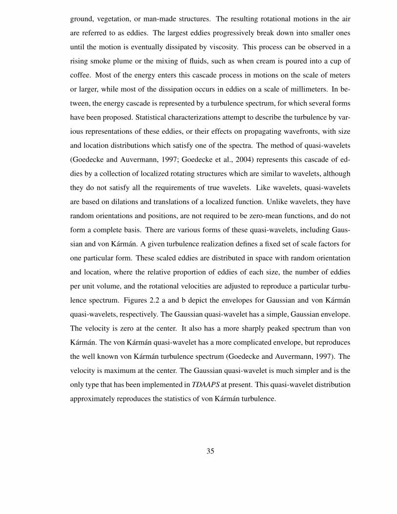
lence spectrum. Figures 2.2 a and b depict the envelopes for Gaussian and von Karman
quasi-wavelets, respectively. The Gaussian quasi-wavelet has a simple, Gaussian envelope.
The velocity is zero at the center. It also has a more sharply peaked spectrum than von
Karman. The von Karman quasi-wavelet has a more complicated envelope, but reproduces
the well known von Karman turbulence spectrum (Goedecke and Auvermann, 1997). The
velocity is maximum at the center. The Gaussian quasi-wavelet is much simpler and is the
only type that has been implemented in TDAAPS at present. This quasi-wavelet distribution
approximately reproduces the statistics of von Karman turbulence.
35
Figure 2.2. (a) Gaussian and (b) von Karman quasi-wavelets.
The arrowheads indicate the rotational velocity, with the size pro-
portional to the relative magnitude. Actual velocities and spatial
dimensions are determined by appropriate scale factors in order to
reproduce a given turbulence spectrum.
36

2.7 Usage and Definition of Flags
Following is a Backus-Naur Form (BNF) definition (Backus, 1959) of a call of TDAAPS.This is followed by a brief description of each possible flag. Certain experimental optionsare not listed here, but can be obtained by calling TDAAPS–help. Flags are show in bold-face and arguments are shown in italic face. Note that the options to TDAAPS may changein the future. An up to date list of options and arguments can be obtained by running:
> TDAAPS -help
Depending on the details of the operating system being used this command may have to be
run in a parallel environment and the output captured.
2.7.1 BNF Definition of TDAAPS call
vecspec: (start:[inc:]end)|(start inc N)
TDAAPS filename ARGUMENT FILE:filename [-p nx ny nz] [-C vecspec directory]
[-bF][-bV] [-bS nodes value] [-R[1] type x y z amplitude [θ φ]] [-R(v|d|a)][-Ru]
[-Rg type x-vecspec y-vecspec z-vecspec] [-Rf[3] type filename] [-Sw filename] [-Sr[0] frequency] [-Su] [-Sf x y z amplitude θ φ] [-Se x y z amplitude] [-Sm x y z
amplitude xx xy xz yx yy yz zx zy zz] [-Es time component plane coordinate] [-Ennumber component plane coordinate] [-Eo filename] [-Mp direction u∗ z0] [-Mcvx vy] [-Mg z0 ∂vx/∂z ∂vy/∂z vx0 vy0] [-Mf filename] [-M1 filename] [-Mq (auto|none|count)[outer][inner][dissipation rate]] [-Mqh][-Mqp value] [-Mqf filename][-Mqv iterations]
2.7.2 Description of TDAAPS flags
filename: Name of the atmospheric model (NetCDF) file. Note that this file is directly
read by the sub-domain processes; it must be accessible and specified with a full
37
UNIX pathname.
ARGUMENT FILE:filename: Read additional arguments from filename. This can be
any combination of additional ARGUMENT FILE: arguments and flags. Avoid
circular references or undefined results will occur. This is useful to avoid extremely
long command lines.
-p nx ny nz: Set the parallel domain decomposition in the x, y, and z directions. Note,
since TDAAPS uses a master-slave paradigm, the the total number of processes will
be nx ∗ny ∗nz +1.
-t count: Write the trace output after this many iterations. This is useful to record early
results if the simulation is going unstable in later iterations.
-C vecspec: Add checkpoints at iterations specified by the vecspec. Data will be written
into the user specified directory which must already exist. If TDAAPS is re-started
with the same model and exactly the same command line it will look for a previ-
ously written checkpoint. If one is present, the run will start from the time of the
checkpoint.
-bF: Use a pressure free surface at the top of the model. The surface is actually at zmin +
2dz.
-bV: Use a rigid (zero wz) surface at the top of the model. The surface is actually at
zmin +2dz.
-bS nodes value: Use a spongy boundary in addition to the off center derivatives on the
model flanks. The default settings are 25 nodes with a final taper value of 95%. Note
that -bF|V automatically turns off any sponge at zmin.
-R*: Flags that deal with defining receivers:
-R[1] type x y z amp [theta phi]: Add one receiver at the given location. Type must
be one of: Velocity, Pressure, 3C, or 4C. If type is “Velocity” θ and φ specify
38
the orientation. Type “3C” is a set of three velocity receivers in the x, y, and z
directions. Type “4C” also includes a pressure receiver.
-R(v|d|a): Subsequent velocity receivers will record: velocity (default), displace-
ment (integrated velocity), or acceleration (differentiated velocity).
-Ru: Subsequent velocity receiver directions specified in radians (default is de-
grees).
-Rg type x-vecspec y-vecspec-zvecspec: Add a grid of receivers. Type must be one
of: “Vx”, “Vy”, “Vz”, “Pressure”, “3C”, or “4C”.
-Rf[3] filename: Add receivers from locations specified in file. Type must be one
of: “Vx”, “Vy”, “Vz”, “Pressure”, “3C”, or “4C”. Each line of the file should
consist of 4 numbers: x location, y location, z location, amplitude. If the option
3 is present skip the amplitude and it will be set to unity.
-S*: Flags that deal with defining sources:
-Sw filename: Read a source wavelet from file.
-Sr F: Generate a Ricker wavelet with given central frequency. Note that -Sw or
-Sr must be used before any sources can be defined.
-Su: Subsequent source directions specified in radians (default is degrees).
-Sf x y z amp theta phi: Add a force source at the specified location and direction.
θ is measured from the z-axis, φ is measured from the x-axis.
-Se x y z amp: Add an explosive source.
-Sm x y z amp axx axy axz ayx ayy ayz azx azy azz : Add a general moment source with
user defined values.
-E*: Flags that deal with extra output:
-Eo filename: Time-slice output file.
-Es time component plane coordinate: Add a single slice at the given time.
39
-En number component plane coordinate: Add n slices evenly distributed through
the run.
-M*: Flags that deal with defining the moving-medium:
-Mp direction u∗ z0: Create a logarithmic wind profile of the form w(z) = u∗log( zz0
).
Note that this also sets up a height dependent quasi-wavelet distribution unless
it is followed by -Mq none.
-Mc vx vy: Build a constant horizontal wind with the given vx and vy.
-Mg z0∂vx∂z
∂vy∂z vx0 vy0: Build a horizontal wind model with a gradient in z.
-Mf filename: Read a 3D wind field from the NetCDF file specified. The file mustcontain variables to define the three components of the wind velocity.
-M1 filename: Read a 2D wind field for the text file specified. This file should have
three columns of z, vx, and vy. If the last z value does not reach the top of the
model the final value is upward continued.
-Mq*: Options to control the use of quasi-wavelets:
-Mq (auto|none|count)[outer][inner][dissipation rate]: Use (or don’t use with
the none option) quasi-wavelets. With the user specified inner and outer
radii and dissipation rate.
-Mqh: Make the quasi-wavelet distribution height dependent.
-Mqp value: If the number of quasi-wavelets is auto this controls the number
of quasi-wavelets generated.
-Mqf filename: Read (if quasi-wavelet generation has not been enabled) or
write the quasi-wavelet distribution. This makes it possible for successive
runs to use identical quasi-wavelet distributions.
-Mqv iterations: Update quasi-wavelet locations. The locations are moved
with the background velocity in jumps when this number of iterations have
passed.
40
Chapter 3
Model Generation
3.1 Introduction
A significant technical challenge in performing acoustic modeling of realistic atmospheric
scenarios is the generation of the atmospheric model. An acoustic atmospheric model is
defined by five parameters; TDAAPS assumes those parameters are c, ρ, and v (acoustic
velocity, density, and the 3 components of the wind velocity, respectively).
The atmospheric model actually consists of several parts: (1) a description of the model
size–this includes the number of nodes in the x, y, and z directions and the number of time-
steps. The model size information also includes the increments and starting point for each
of these four dimensions. (2) The wavespeed and densities at each of the grid-points in the
xyz grid. (3) A definition of the recording geometry (if any)–this is the number and layout
of the receivers. (4) A definition of the sources. (5) A definition of extra output (i.e. time
slice output). The first two parts are required and all the additional parts are optional (these
can be specified on the TDAAPS command line if desired).
There are two distinct methods of building model files that are described in this chapter:
the first uses MatlabTM directly, and the second uses the program buildSgfdModel.
41
3.2 Model Building with MatlabTM
This is probably the easiest method to understand and illustrate. Over time the author hasmoved most model-building tasks to this environment. The use of MatlabTM to build themost trivial model possible was illustrated in Section 2.3. To reduce repetitive chores thefollowing (long) MatlabTM function provides tools for basic model definition (with someextra variables defined to simplify later examination of the data):
1 function writeSgfdModel(filename,x,y,z,t,varargin)%function writeSgfdModel(filename,x,y,z,t,varargin)%Write a Symons style netcdf file for sgfd modeling. Can be used for either% elastic or acoustic models.%Neill Symons; Sandia National Laboratories; 4/24/03%Arguments: filename--file to write% x, y, z--vectors with spatial position of node centers% t--time vector.%Optional Arguments: vp, vs, rho--these are done optionally for some
10 % flexability in what is actually defined.% comment--add a comment to the file% noclobber--add variables to an exisiting file, useful% for large models.% NOTE: because of the way NetCDF stores variables% size(vp,1)==length(z)% size(vp,2)==length(y)% size(vp,3)==length(x)%
20 %Check varargin for modifiers to the default arguments.i=1;while i<=length(varargin)
currArg=varargini;i=i+1;argType=whos(’currArg’);if ˜strcmp(argType.class,’char’)
error(sprintf(’Optional argument %i, type %s must be char’,...i,argType.class));
end30
switch lower(currArg)case ’velocity’ ’vel’ ’vp’ ’v’ ’alpha’ ’c’
vp=varargini;i=i+1;
case ’density’ ’rho’rho=varargini;i=i+1;
case ’slice’40 sliceName=varargini;
sliceTimes=varargini+1;slicePos=varargini+2;i=i+3;if exist(’slices’)˜=1numSlices=length(sliceTimes);slices=sliceName,sliceTimes,slicePos;
elsenumSlices=numSlices+length(sliceTimes);slices=slices: sliceName,sliceTimes,slicePos;
50 endclear sliceName sliceTimes slicePos;
case ’pressurereceivers’
42
receiverX=varargini+0;receiverY=varargini+1;receiverZ=varargini+2;i=i+3;receiverType=2+0*receiverX;
60 receiverAmp=1+0*receiverX;receiverBx=0*receiverX;receiverBy=0*receiverX;receiverBz=0*receiverX;receiverIntegrate=0*receiverX;
case ’source’ ’pressuresource’ ’explosion’pressureSource=varargini;sourceWaveform=varargini+1;
70 i=i+2;case ’comment’
comment=varargini;i=i+1;
case ’history’history=varargini;i=i+1;
case ’noclobber’ ’addvar’ ’add’80 %Add a new time plane to an existing file.
noclobber=1;otherwise
error(sprintf(’Unknown option %s’,currArg));end
end%Check that the sizes match up.NX=length(x);
90 NY=length(y);NZ=length(z);NT=length(t);if exist(’vp’)==1 & (...
size(vp,1)˜=NZ | size(vp,2)˜=NY | size(vp,3)˜=NX)fprintf(’Because of the way NetCDF stores variables\n’);fprintf(’ size(vp,1)==length(z)\n’);fprintf(’ size(vp,2)==length(y)\n’);fprintf(’ size(vp,3)==length(x)\n’);
100 error(’Can not write file’);endif exist(’rho’)==1 & (...
size(rho,1)˜=NZ | size(rho,2)˜=NY | size(rho,3)˜=NX)fprintf(’Because of the way NetCDF stores variables\n’);fprintf(’ size(rho,1)==length(z)\n’);fprintf(’ size(rho,2)==length(y)\n’);fprintf(’ size(rho,3)==length(x)\n’);error(’Can not write file’);
110 end%Open the file.if exist(’noclobber’)==1 & noclobber
out=netcdf(filename,’write’);else
out=netcdf(filename,’clobber’);%Set some global attribute describing how this file was created.out.title=’Staggered Grid Finite-Difference Model Input File’;
120 if exist(’comment’)==1out.comment=comment;
endif exist(’history’)==1
out.history=history;
43
elseout.history=’Created with matlab writeSgfdModel.m’;
end%Set the dimensions.
130 out(’numCoord’)=4;out(’NX’)=NX;out(’NY’)=NY;out(’NZ’)=NZ;out(’NT’)=NT;%Define and fill the increment variables.out’minima’=ncfloat(’numCoord’);out’minima’(:)=[x(1) y(1) z(1) t(1)];out’increments’=ncfloat(’numCoord’);
140 out’increments’(:)=[x(2)-x(1) y(2)-y(1) z(2)-z(1) t(2)-t(1)];%Define and fill the position variables.out’x’=ncfloat(’NX’);out’x’(:)=x;out’y’=ncfloat(’NY’);out’y’(:)=y;out’z’=ncfloat(’NZ’);out’z’(:)=z;out’time’=ncfloat(’NT’);
150 out’time’(:)=t;end%Write the defined variables.if exist(’vp’)==1
out’vp’=ncfloat(’NZ’,’NY’,’NX’);out’vp’(:)=vp;
endif exist(’rho’)==1
out’rho’=ncfloat(’NZ’,’NY’,’NX’);160 out’rho’(:)=rho;
end%%Write extra defined stuff.%%Slices.if exist(’slices’)==1
out(’numSlices’)=numSlices;170
out’sliceTime’=ncfloat(’numSlices’);out’sliceComp’=ncint(’numSlices’);out’slicePlane’=ncint(’numSlices’);out’sliceCoord’=ncfloat(’numSlices’);startSlice=0;for i=1:length(slices)
currSlice=slicesi;sliceName=currSlice1;
180 sliceTimes=currSlice2;sliceCoord=currSlice3;out’sliceTime’(startSlice+1:startSlice+length(sliceTimes))=sliceTimes;for i=1:length(sliceTimes)
out’sliceCoord’(i+startSlice)=sliceCoord;switch lower(sliceName(1:2))case ’yz’
out’slicePlane’(i+startSlice)=1;if x(1)>sliceCoord | sliceCoord>x(end)
190 error(’Slice %s: out of bounds %f<%f<%f’,...sliceName,x(1),sliceCoord,x(end));
endcase ’xz’
out’slicePlane’(i+startSlice)=2;if y(1)>sliceCoord | sliceCoord>y(end)
error(’Slice %s: out of bounds %f<%f<%f’,...sliceName,y(1),sliceCoord,y(end));
44
endcase ’xy’
200 out’slicePlane’(i+startSlice)=3;if z(1)>sliceCoord | sliceCoord>z(end)
error(’Slice %s: out of bounds %f<%f<%f’,...sliceName,z(1),sliceCoord,z(end));
endotherwise
error(sprintf(’Unknown slice plane %s’,sliceName(1:2)));endswitch lower(sliceName(3:end))
210 case ’vx’out’sliceComp’(i+startSlice)=1;
case ’vy’out’sliceComp’(i+startSlice)=2;
case ’vz’out’sliceComp’(i+startSlice)=3;
case ’pressure’out’sliceComp’(i+startSlice)=4;
otherwiseerror(sprintf(’Unknown slice component %s’,sliceName(3:end)));
220 endendstartSlice=startSlice+length(sliceTimes);
endend%Receivers.if exist(’receiverType’)==1
out(’numReceivers’)=length(receiverType);230
out’receiverType’=ncint(’numReceivers’);out’receiverAmp’=ncfloat(’numReceivers’);out’receiverX’=ncfloat(’numReceivers’);out’receiverY’=ncfloat(’numReceivers’);out’receiverZ’=ncfloat(’numReceivers’);out’receiverBx’=ncfloat(’numReceivers’);out’receiverBy’=ncfloat(’numReceivers’);out’receiverBz’=ncfloat(’numReceivers’);out’receiverIntegrate’=ncint(’numReceivers’);
240out’receiverType’(:)=receiverType;out’receiverAmp’(:)=receiverAmp;out’receiverX’(:)=receiverX;out’receiverY’(:)=receiverY;out’receiverZ’(:)=receiverZ;out’receiverBx’(:)=receiverBx;out’receiverBy’(:)=receiverBy;out’receiverBz’(:)=receiverBz;
250 out’receiverIntegrate’(:)=receiverIntegrate;end%Sources.if exist(’pressureSource’)==1
out(’numMSources’)=1;out’mSourcesXs’=ncfloat(’numMSources’);out’mSourcesYs’=ncfloat(’numMSources’);out’mSourcesZs’=ncfloat(’numMSources’);
260out’mSourcesSamp’=ncfloat(’numMSources’);out’mSourcesXxS’=ncfloat(’numMSources’);out’mSourcesYyS’=ncfloat(’numMSources’);out’mSourcesZzS’=ncfloat(’numMSources’);out’mSourcesXyS’=ncfloat(’numMSources’);out’mSourcesXzS’=ncfloat(’numMSources’);out’mSourcesYzS’=ncfloat(’numMSources’);
45
270out’mSourcesXyA’=ncfloat(’numMSources’);out’mSourcesXzA’=ncfloat(’numMSources’);out’mSourcesYzA’=ncfloat(’numMSources’);out’mSourcesXs’(1)=pressureSource(1);out’mSourcesYs’(1)=pressureSource(2);out’mSourcesZs’(1)=pressureSource(3);out’mSourcesSamp’(1)=1;
280out’mSourcesXxS’(1)=1;out’mSourcesYyS’(1)=1;out’mSourcesZzS’(1)=1;out’mSourcesXyS’(1)=0;out’mSourcesXzS’(1)=0;out’mSourcesYzS’(1)=0;out’mSourcesXyA’(1)=0;
290 out’mSourcesXzA’(1)=0;out’mSourcesYzA’(1)=0;out’mSourcesData’=ncfloat(’numMSources’,’NT’);out’mSourcesData’(1,:)=sourceWaveform;
end%Close the file.close(out);
The following function illustrates a methodology whereby sources, receivers, and time-slices can be defined with the MatlabTM model generation methods. The writeSgfdModelfunction is used to generate the model for the transmission loss over a hill part of the Alphatest. The MatlabTM code to create this model is:
1 function [mName]=build_hill_model(dx,varargin)%% Define the parameters of the model buildif nargin<1
dx=0.50;enddt=1e-4*dx;maxT=2.0;standoff=8;
10 offset=25*dx;soffset=50*dx;minUX=100;minX=-minUX-soffset;maxX=minUX+offset;yrange=40+offset;minZ=-soffset;maxZ=60+offset;
20 %% Define the parameters of the cylindrical hill.center=[0 -200];radius=sqrt(center(2)ˆ2+minUXˆ2);%% Build vectors for the axes.x=[minX:dx:maxX];y=[-yrange:dx:yrange];z=[minZ:dx:maxZ];t=[0:dt:maxT];
30NX=length(x);NY=length(y);
46
NZ=length(z);NT=length(t);%% Build vectors for the receiver array and source.re=5;rx=[-minUX+10:5:minUX];ry=0*rx;
40 rz=sqrt((radius+re)ˆ2-rx.ˆ2)+center(2);sl=[-minUX 0 sqrt((radius+re)ˆ2-minUX.ˆ2)+center(2)];sw=monofreq(100,dt,length(t));%clear offset soffset minUX minX maxX yrange minZ maxZ;%% Write the basic model.mName=’BetaHill1.cdf’;writeSgfdModel(mName,x,y,z,t,...
50 ’comment’,sprintf(’Version 1.0: dx=%.1f; dt=%5g’,dx,dt),...’history’,textFromFile(’build_hill_model.m’),...’pressurereceivers’,rx,ry,rz,...’pressuresource’,sl,sw);
out=netcdf(mName,’write’);out.title=’TDAPS Beta Test Hill Model Input File’;%% And fill in the variables.[Y,Z,X]=meshgrid(y,z,x);
60 D=sqrt(X.ˆ2+(Z-center(2)).ˆ2);%% Define a variable for vp and fill it in. Make sure the rock does% not intersect with the edge of the model.out’vp’=ncfloat(’NZ’,’NY’,’NX’);vp=342*ones(NZ,NY,NX);vp(D<=radius &...
X>(minX+standoff*dx) & X<(maxX-standoff*dx) & ...Y>(-yrange+standoff*dx) & Y<(yrange-standoff*dx) &...
70 Z>(minZ+standoff*dx))=3500;out’vp’(:,:,:)=vp;%% Define a variable for rho and fill it in.% Be careful that all nodes on a transition from rock to air are% filled with intermediate properties. This includes diagional% contacts.out’rho’=ncfloat(’NZ’,’NY’,’NX’);rho=1.2*ones(NZ,NY,NX);rho(vp>1000)=2000;
80 for i=1:NXfor j=1:NY
for k=1:NZ-1if rho(k,j,i)>10modify=0;for ii=max(1,i-1):min(NX,i+1)
for jj=max(1,j-1):min(NY,j+1)for kk=max(1,k-1):min(NZ,k+1)if vp(kk,jj,ii)<1000
modify=1;90 end
endend
endif modify
rho(k,j,i)=100;end
endend
end100 end
out’rho’(:,:,:)=rho;%% Close the file.close(out);
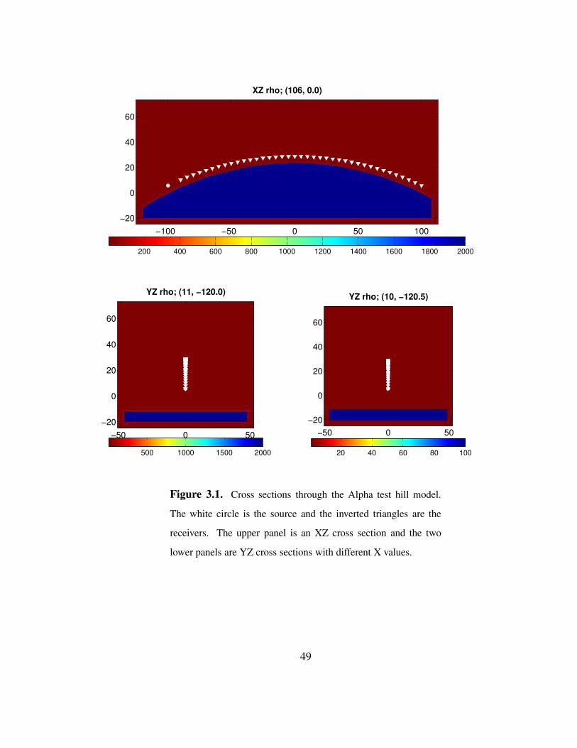
47
The model that results from the execution of this script is shown in Figure 3.1. This models
uses the material contrast pseudo-boundary-condition described in Section 2.5.2.
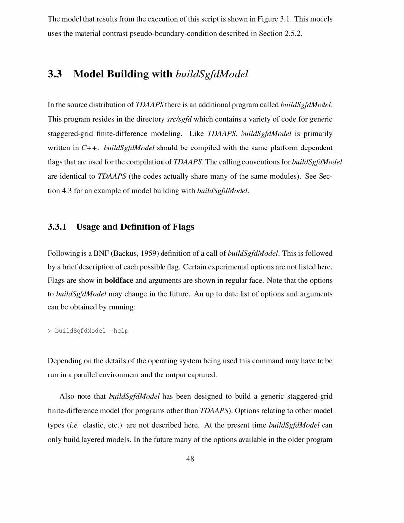
3.3 Model Building with buildSgfdModel
In the source distribution of TDAAPS there is an additional program called buildSgfdModel.
This program resides in the directory src/sgfd which contains a variety of code for generic
staggered-grid finite-difference modeling. Like TDAAPS, buildSgfdModel is primarily
written in C++. buildSgfdModel should be compiled with the same platform dependent
flags that are used for the compilation of TDAAPS. The calling conventions for buildSgfdModel
are identical to TDAAPS (the codes actually share many of the same modules). See Sec-
tion 4.3 for an example of model building with buildSgfdModel.
3.3.1 Usage and Definition of Flags
Following is a BNF (Backus, 1959) definition of a call of buildSgfdModel. This is followedby a brief description of each possible flag. Certain experimental options are not listed here.Flags are show in boldface and arguments are shown in regular face. Note that the optionsto buildSgfdModel may change in the future. An up to date list of options and argumentscan be obtained by running:
> buildSgfdModel -help
Depending on the details of the operating system being used this command may have to be
run in a parallel environment and the output captured.
Also note that buildSgfdModel has been designed to build a generic staggered-grid
finite-difference model (for programs other than TDAAPS). Options relating to other model
types (i.e. elastic, etc.) are not described here. At the present time buildSgfdModel can
only build layered models. In the future many of the options available in the older program
48
200 400 600 800 1000 1200 1400 1600 1800 2000
XZ rho; (106, 0.0)
−100 −50 0 50 100−20
0
20
40
60
500 1000 1500 2000
YZ rho; (11, −120.0)
−50 0 50−20
0
20
40
60
20 40 60 80 100
YZ rho; (10, −120.5)
−50 0 50−20
0
20
40
60
Figure 3.1. Cross sections through the Alpha test hill model.
The white circle is the source and the inverted triangles are the
receivers. The upper panel is an XZ cross section and the two
lower panels are YZ cross sections with different X values.
49
generateModel (not described here) may also be implemented. However, the author has
found that the vast majority of complex models are now constructed directly in MatlabTM.
3.3.2 BNF Definition of buildSgfdModel call
vecspec: (start:[inc:]end)|(start inc N)
buildSgfdModel acoustic filename ARGUMENT FILE:filename [-xvecspec] [-yvecspec]
[-zvecspec] [-tvecspec] [-I] [-mlthickness c rho] [-R[1] type x y z amplitude [θ φ]]
[-R(v|d|a)][-Ru] [-Rg type x-vecspec y-vecspec z-vecspec] [-Rf[3] type filename] [-Sw filename] [-Sr[0] frequency] [-Su] [-Sf x y z amplitude θ φ] [-Se x y z amplitude]
[-Sm x y z amplitude xx xy xz yx yy yz zx zy zz] [-Es time component plane coordinate]
[-En number component plane coordinate]
3.3.3 Description of buildSgfdModel flags
filename: Name of the atmospheric model (NetCDF) file.
ARGUMENT FILE:filename: Read additional arguments from filename. This can be
any combination of additional ARGUMENT FILE: arguments and flags. Avoid
circular references or undefined results will occur. This is useful to avoid extremely
long command lines.
-I: Create an indexed model. At preset this is always a 1D model (see Section 2.3).
-x|y|z|t vecspec: Define the given axis. See Section 2.7.1 for a definition of the vecspec.
-ml thickness c rho: Define a new layer with the given thickness and properties.
-R*: Flags that deal with defining receivers: see section 2.7.2 for details.
-S*: Flags that deal with defining sources: see section 2.7.2 for details.
-E*: Flags that deal extra output:see section 2.7.2 for details.
50
Chapter 4
Examples
This chapter contains several examples of using TDAAPS to run a variety of simulations.
These simulations are of varying complexity and are drawn primarily from the suite of tests
required for the Alpha and Beta tests. These examples have been modified to simplify and
shorten the scripts. Complete “as run” examples may be found in Appendices B and C.
4.1 Transmission Loss with Vertical Wind Gradient
An Alpha test goal was that the transmission loss modeled by TDAAPS over a perfectly
hard flat ground in a moving refractive atmosphere would be within 1 dB of a benchmarked
wavenumber integration scheme at a range of 200m and 100Hz frequency. The atmospheric
model for this test was a constant acoustic velocity half-space (c 342m/s and ρ 1.2Kg/m3)
over a zero wz hard surface. The refractive atmosphere was provided with a linear wind
speed gradient from 0m/s at the surface increasing by 0.1(m/s)/m in the vertical direction.
The model was 901× 201 × 203(∼ 36M) nodes with a 0.5m grid spacing for a total
dimension of −225m to 225m in x, −50m to 50m in y, and −1m to 100m in z. The time-
step is 0.25ms and the total model-time was 2s, therefore implying 8001 time-steps. The
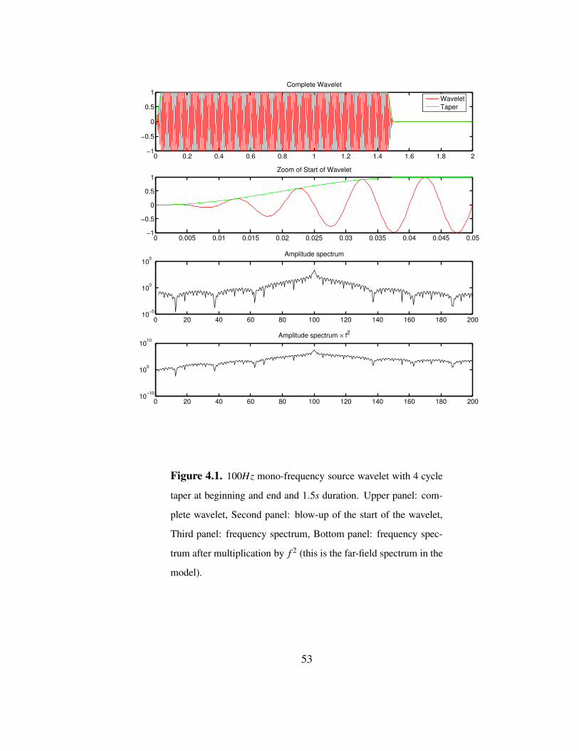
source is a monopole of 100Hz with a four cycle taper (Figure 4.1) at the beginning and
51
end to limit the high frequencies introduced into the model.
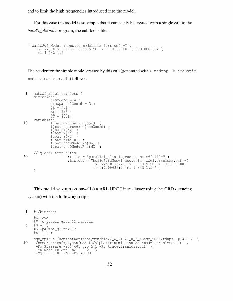
For this case the model is so simple that it can easily be created with a single call to thebuildSgfdModel program, the call looks like:
> buildSgfdModel acoustic model.tranloss.cdf -I \-x -225:0.5:225 -y -50:0.5:50 -z -1:0.5:100 -t 0:0.00025:2 \-ml 1 342 1.2
The header for the simple model created by this call (generated with > ncdump -h acoustic
model.tranloss.cdf) follows:
1 netcdf model.tranloss dimensions:
numCoord = 4 ;numSpatialCoord = 3 ;NX = 901 ;NY = 201 ;NZ = 203 ;NT = 8001 ;
variables:10 float minima(numCoord) ;
float increments(numCoord) ;float x(NX) ;float y(NY) ;float z(NZ) ;float time(NT) ;float oneDModelVp(NZ) ;float oneDModelRho(NZ) ;
// global attributes:20 :title = "parallel_elasti generic NETcdf file" ;
:history = "buildSgfdModel acoustic model.tranloss.cdf -I-x -225:0.5:225 -y -50:0.5:50 -z -1:0.5:100-t 0:0.00025:2 -ml 1 342 1.2 " ;
This model was run on powell (an ARL HPC Linux cluster using the GRD queueingsystem) with the following script:
1 #!/bin/tcsh#$ -cwd#$ -o powell_grad_01.run.out
5 #$ -j y#$ -pe mpi_glinux 17#$ -l 4hrsge_mpirun /home/others/npsymon/bin/2_4_21-27_0_2_ELsmp_i686/tdaps -p 4 2 2 \
10 /home/others/npsymon/models/Alpha/TransmissionLoss/model.tranloss.cdf \-Rg Pressure -200:401 0:0 5:5 -Ro trace.tranloss.cdf \-Sw mono100.out -Se 0 0 2 1 \-Mg 0 0.1 0 -bV -bS 40 90
52
0 0.2 0.4 0.6 0.8 1 1.2 1.4 1.6 1.8 2−1
−0.5
0
0.5
1Complete Wavelet
0 0.005 0.01 0.015 0.02 0.025 0.03 0.035 0.04 0.045 0.05−1
−0.5
0
0.5
1Zoom of Start of Wavelet
0 20 40 60 80 100 120 140 160 180 20010−5
100
105Amplitude spectrum
0 20 40 60 80 100 120 140 160 180 20010−10
100
1010Amplitude spectrum × f2
WaveletTaper
Figure 4.1. 100Hz mono-frequency source wavelet with 4 cycle
taper at beginning and end and 1.5s duration. Upper panel: com-
plete wavelet, Second panel: blow-up of the start of the wavelet,
Third panel: frequency spectrum, Bottom panel: frequency spec-
trum after multiplication by f 2 (this is the far-field spectrum in the
model).
53
The comments in the first 7 lines of the script set the queue parameters for a 4×
2× 2(16) processors run and send the output to the file “powell grad 01.run.out”. Line
9 is the call to the executable and sets the decomposition. Line 10 sets the model to
“/home/others/npsymon/models/Alpha/TransmissionLoss/model.tranloss.cdf”. Line 10 de-
fines a line of receivers along the x-axis from -200 to 200m at 1m increments and sets the
trace output filename to “trace.tranloss.cdf”. Line 11 reads the source waveform from
“mono100.out” and sets the monopole source at (0,0,2)m with a scalar amplitude of unity.
Line 12 sets the wind gradient, the zero wz boundary condition, and then sets a 40 node
wide absorbing boundary around the model with a value that tapers to 90%. More details
about the available flags to modify the behavior of TDAAPS is in Section 3.3.3.
The output from this example is shown in a record section in Figure 4.2. Note the asym-
metry in the magnitude of the pressure between the receivers at −200 and 200m because
of the refractive atmosphere.
4.2 Extinction and Coherence
This section describes the modeling for the Alpha test extinction and coherence test (thecomplete unmodified Beta test results can be seen in Section B.2). The model for this testwas a whole space with c 342m/s and ρ 1.2Kg/m3. This model is 651× 651× 651(∼
275M) nodes with a 0.5m grid spacing. The x, y, and z grids all range from -80m to 245m.The random receiver locations are read into the model from a file generated in MatlabTM
with the following simple script:
1 %Create the random distribution.rL0=rand(500,3);%Create a vector that can be used to normalize the distance of each
5 %receiver from the origin.rL0L=sqrt(rL0(:,1).ˆ2+rL0(:,2).ˆ2+rL0(:,3).ˆ2);%Divide by the length from the origin and multiply to 200 to put each%receiver on a 200m radius sphere.
10 for i=1:500;rL(i,:)=200*rL0(i,:)/rL0L(i);
end
These locations are then written out to a file in a 3 column format. The source and a
54
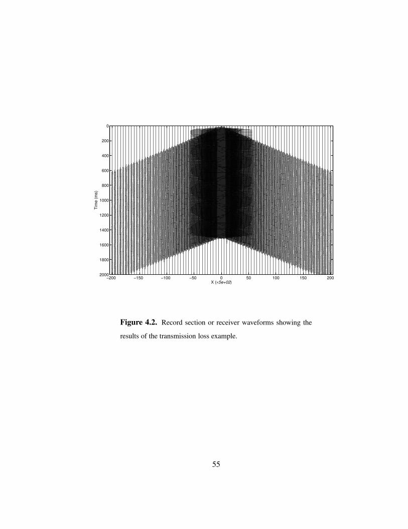
−200 −150 −100 −50 0 50 100 150 200
0
200
400
600
800
1000
1200
1400
1600
1800
2000X (×5e+02)
Tim
e (m
s)
Figure 4.2. Record section or receiver waveforms showing the
results of the transmission loss example.
55
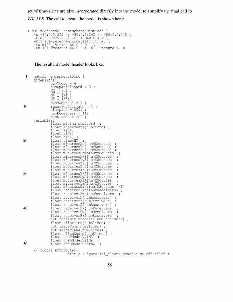
set of time-slices are also incorporated directly into the model to simplify the final call toTDAAPS. The call to create the model is shown here:
> buildSgfdModel hemisphereRDist.cdf \-x -80:0.5:245 -y -80:0.5:245 -z -80:0.5:245 \-t 0:0.00025:2 -I -ml 1 340 0 1.2 \-Rf3 Pressure hemisphereR11_11.txt \-Sw m100_15.txt -Se 0 0 0 1 \-En 101 Pressure XZ 0 -En 101 Pressure YZ 0
The resultant model header looks like:
1 netcdf hemisphereRDist dimensions:
numCoord = 4 ;numSpatialCoord = 3 ;NX = 651 ;NY = 651 ;NZ = 651 ;NT = 8001 ;numMSources = 1 ;
10 receiverDecimate = 1 ;nSamples = 8001 ;numReceivers = 111 ;numSlices = 202 ;
variables:float minima(numCoord) ;float increments(numCoord) ;float x(NX) ;float y(NY) ;float z(NZ) ;
20 float time(NT) ;float mSourcesXs(numMSources) ;float mSourcesYs(numMSources) ;float mSourcesZs(numMSources) ;float mSourcesSamp(numMSources) ;float mSourcesXxS(numMSources) ;float mSourcesYyS(numMSources) ;float mSourcesZzS(numMSources) ;float mSourcesXyS(numMSources) ;float mSourcesXzS(numMSources) ;
30 float mSourcesYzS(numMSources) ;float mSourcesXyA(numMSources) ;float mSourcesXzA(numMSources) ;float mSourcesYzA(numMSources) ;float mSourcesData(numMSources, NT) ;float receiverType(numReceivers) ;float receiverAmp(numReceivers) ;float receiverX(numReceivers) ;float receiverY(numReceivers) ;float receiverZ(numReceivers) ;
40 float receiverBx(numReceivers) ;float receiverBy(numReceivers) ;float receiverBz(numReceivers) ;int receiverIntegrate(numReceivers) ;float sliceTime(numSlices) ;int sliceComp(numSlices) ;int slicePlane(numSlices) ;float sliceCoord(numSlices) ;float oneDModelVp(NZ) ;float oneDModelVs(NZ) ;
50 float oneDModelRho(NZ) ;// global attributes:
:title = "parallel_elasti generic NETcdf file" ;
56
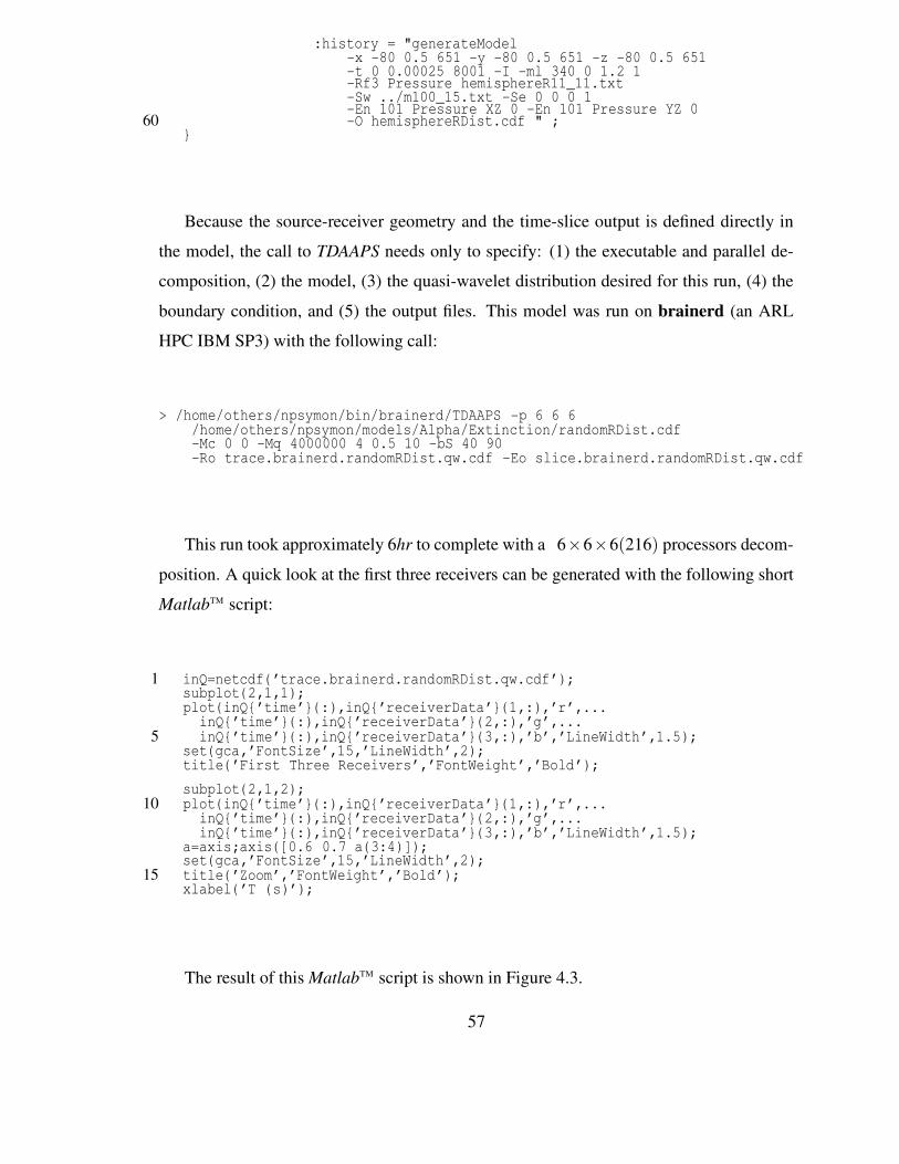
:history = "generateModel-x -80 0.5 651 -y -80 0.5 651 -z -80 0.5 651-t 0 0.00025 8001 -I -ml 340 0 1.2 1-Rf3 Pressure hemisphereR11_11.txt-Sw ../m100_15.txt -Se 0 0 0 1-En 101 Pressure XZ 0 -En 101 Pressure YZ 0
60 -O hemisphereRDist.cdf " ;
Because the source-receiver geometry and the time-slice output is defined directly inthe model, the call to TDAAPS needs only to specify: (1) the executable and parallel de-composition, (2) the model, (3) the quasi-wavelet distribution desired for this run, (4) theboundary condition, and (5) the output files. This model was run on brainerd (an ARLHPC IBM SP3) with the following call:
> /home/others/npsymon/bin/brainerd/TDAAPS -p 6 6 6/home/others/npsymon/models/Alpha/Extinction/randomRDist.cdf-Mc 0 0 -Mq 4000000 4 0.5 10 -bS 40 90-Ro trace.brainerd.randomRDist.qw.cdf -Eo slice.brainerd.randomRDist.qw.cdf
This run took approximately 6hr to complete with a 6×6×6(216) processors decom-position. A quick look at the first three receivers can be generated with the following shortMatlabTM script:
1 inQ=netcdf(’trace.brainerd.randomRDist.qw.cdf’);subplot(2,1,1);plot(inQ’time’(:),inQ’receiverData’(1,:),’r’,...
inQ’time’(:),inQ’receiverData’(2,:),’g’,...5 inQ’time’(:),inQ’receiverData’(3,:),’b’,’LineWidth’,1.5);
set(gca,’FontSize’,15,’LineWidth’,2);title(’First Three Receivers’,’FontWeight’,’Bold’);subplot(2,1,2);
10 plot(inQ’time’(:),inQ’receiverData’(1,:),’r’,...inQ’time’(:),inQ’receiverData’(2,:),’g’,...inQ’time’(:),inQ’receiverData’(3,:),’b’,’LineWidth’,1.5);
a=axis;axis([0.6 0.7 a(3:4)]);set(gca,’FontSize’,15,’LineWidth’,2);
15 title(’Zoom’,’FontWeight’,’Bold’);xlabel(’T (s)’);
The result of this MatlabTM script is shown in Figure 4.3.
57
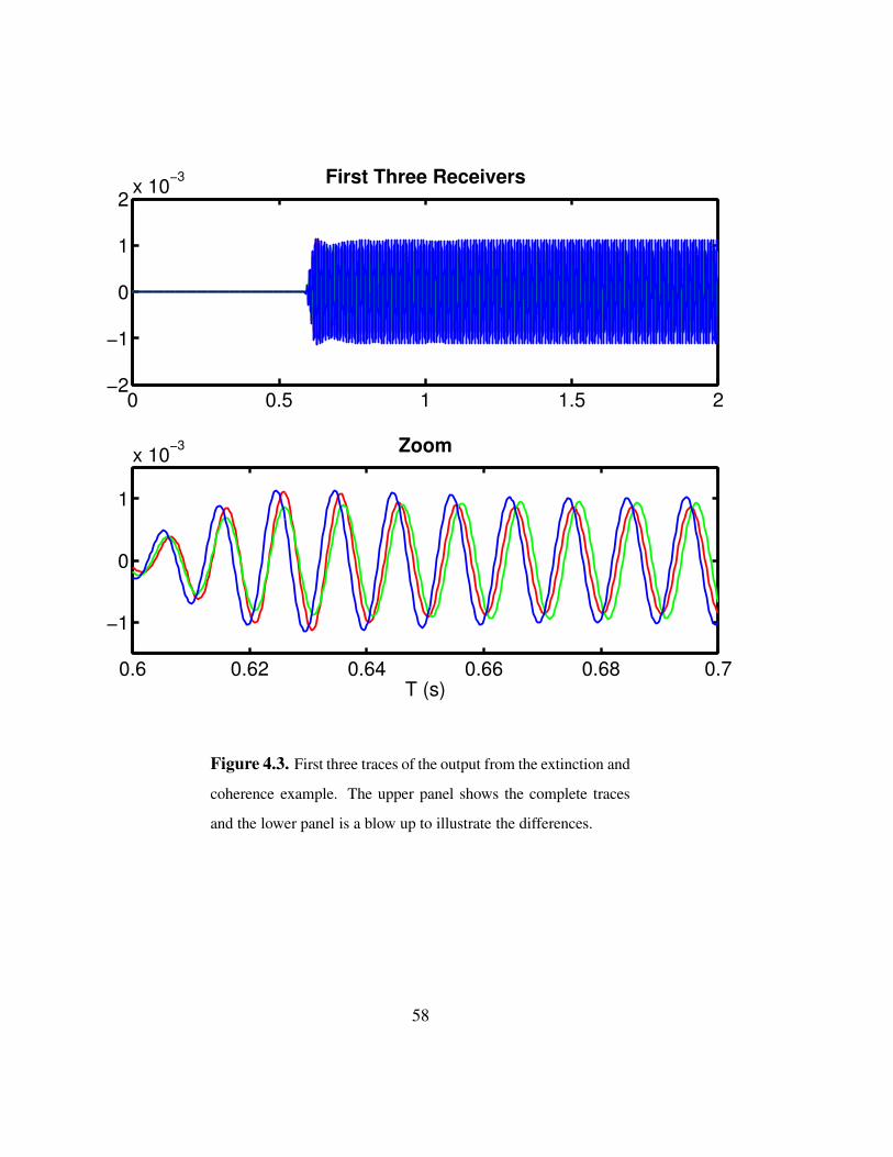
0 0.5 1 1.5 2−2
−1
0
1
2 x 10⁻³ First Three Receivers
0.6 0.62 0.64 0.66 0.68 0.7
−1
0
1
x 10−3 Zoom
T (s)
Figure 4.3. First three traces of the output from the extinction and
coherence example. The upper panel shows the complete traces
and the lower panel is a blow up to illustrate the differences.
58
4.3 Alpha Test Scalability
This section describes the building and running of models for the Alpha test scalabilitydemonstration. Because many runs are needed for this demonstration, a high degree ofautomation is required. Since this is a scaled speedup test. we create a different modelfor each decomposition tested. There are 17 decompositions: 1× 1× 1(1) processors,2×1×1(2) processors, 2×2×1(4) processors, 2×2×2(8) processors, 3×2×2(12)
processors, 3×3×2(18) processors, 3×3×3(27) processors, 4×3×3(36) processors,4× 4× 3(48) processors, 4× 4× 4(64) processors, 4× 4× 5(80) processors, 4× 5×5(100) processors, 4×5×6(120) processors, 4×6×6(144) processors, 4×6×7(168)
processors, 4× 7× 7(196) processors, 4× 7× 8(224) processors, and 4× 8× 8(256)
processors. All of the models for these decompositions are built very quickly with a pair totcsh scripts that use the buildSgfdModel program (Section 3.3). The first script builds andthen calls a second script to build a single model for a specified decomposition:
1 #!/bin/tcshif ($# < 3) then
echo "USAGE: $0 xProc yProc zProc [no_model][stat]"5 exit
elseset XPROC=$1set YPROC=$2set ZPROC=$3
10 shiftshiftshift
endif15 set MOD_EXE=/home/npsymon/bin/buildSgfdModel
#Set IO charachteristics of runset REC="-Rg Pressure 0 10 ‘expr 1 + 4 \* \( $XPROC - 1 \)‘ 0 0 1 2 0 1"set MOD="models/model.$XPROC_$YPROC_$ZPROC.cdf"
20#Determine the model size.set NX=‘expr 50 \* $XPROC + 1‘set NY=‘expr 50 \* $YPROC + 1‘set NZ=‘expr 50 \* $ZPROC + 1‘
25set SX="-25"set SY=‘expr -25 \* $YPROC‘set SZ="-2"
30 #Create the run script.set MOD_SCRIPT_FILE=scripts/$XPROC_$YPROC_$ZPROC.model.scriptcat > $MOD_SCRIPT_FILE <<EOF#!/bin/tcsh
35 $MOD_EXE -I acoustic\-x $SX 1 $NX -y $SY 1 $NY -z $SZ 1 $NZ \-t 0:0.0005:0.500 -I -ml 1 342 1.2 \-Sw models/m40_00005.txt -Se 0 0 5 1 \$REC \
59
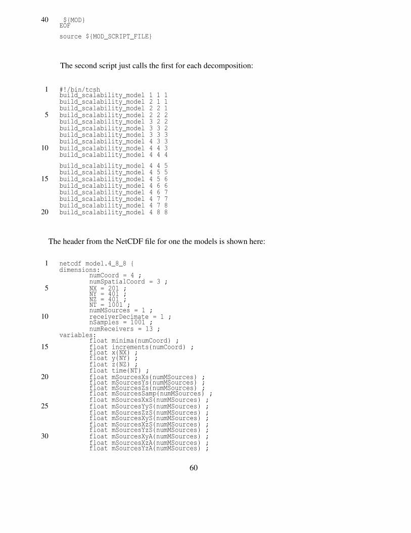
40 $MODEOFsource $MOD_SCRIPT_FILE
The second script just calls the first for each decomposition:
1 #!/bin/tcshbuild_scalability_model 1 1 1build_scalability_model 2 1 1build_scalability_model 2 2 1
5 build_scalability_model 2 2 2build_scalability_model 3 2 2build_scalability_model 3 3 2build_scalability_model 3 3 3build_scalability_model 4 3 3
10 build_scalability_model 4 4 3build_scalability_model 4 4 4build_scalability_model 4 4 5build_scalability_model 4 5 5
15 build_scalability_model 4 5 6build_scalability_model 4 6 6build_scalability_model 4 6 7build_scalability_model 4 7 7build_scalability_model 4 7 8
20 build_scalability_model 4 8 8
The header from the NetCDF file for one the models is shown here:
1 netcdf model.4_8_8 dimensions:
numCoord = 4 ;numSpatialCoord = 3 ;
5 NX = 201 ;NY = 401 ;NZ = 401 ;NT = 1001 ;numMSources = 1 ;
10 receiverDecimate = 1 ;nSamples = 1001 ;numReceivers = 13 ;
variables:float minima(numCoord) ;
15 float increments(numCoord) ;float x(NX) ;float y(NY) ;float z(NZ) ;float time(NT) ;
20 float mSourcesXs(numMSources) ;float mSourcesYs(numMSources) ;float mSourcesZs(numMSources) ;float mSourcesSamp(numMSources) ;float mSourcesXxS(numMSources) ;
25 float mSourcesYyS(numMSources) ;float mSourcesZzS(numMSources) ;float mSourcesXyS(numMSources) ;float mSourcesXzS(numMSources) ;float mSourcesYzS(numMSources) ;
30 float mSourcesXyA(numMSources) ;float mSourcesXzA(numMSources) ;float mSourcesYzA(numMSources) ;
60
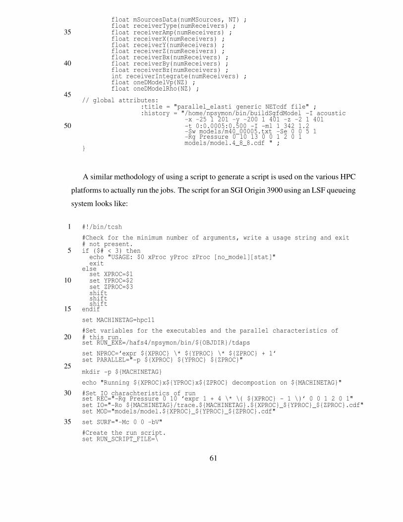
float mSourcesData(numMSources, NT) ;float receiverType(numReceivers) ;
35 float receiverAmp(numReceivers) ;float receiverX(numReceivers) ;float receiverY(numReceivers) ;float receiverZ(numReceivers) ;float receiverBx(numReceivers) ;
40 float receiverBy(numReceivers) ;float receiverBz(numReceivers) ;int receiverIntegrate(numReceivers) ;float oneDModelVp(NZ) ;float oneDModelRho(NZ) ;
45// global attributes:
:title = "parallel_elasti generic NETcdf file" ;:history = "/home/npsymon/bin/buildSgfdModel -I acoustic
-x -25 1 201 -y -200 1 401 -z -2 1 40150 -t 0:0.0005:0.500 -I -ml 1 342 1.2
-Sw models/m40_00005.txt -Se 0 0 5 1-Rg Pressure 0 10 13 0 0 1 2 0 1models/model.4_8_8.cdf " ;
A similar methodology of using a script to generate a script is used on the various HPCplatforms to actually run the jobs. The script for an SGI Origin 3900 using an LSF queueingsystem looks like:
1 #!/bin/tcsh#Check for the minimum number of arguments, write a usage string and exit# not present.
5 if ($# < 3) thenecho "USAGE: $0 xProc yProc zProc [no_model][stat]"exit
elseset XPROC=$1
10 set YPROC=$2set ZPROC=$3shiftshiftshift
15 endifset MACHINETAG=hpc11#Set variables for the executables and the parallel characteristics of
20 # this run.set RUN_EXE=/hafs4/npsymon/bin/$OBJDIR/tdapsset NPROC=‘expr $XPROC \* $YPROC \* $ZPROC + 1‘set PARALLEL="-p $XPROC $YPROC $ZPROC"
25mkdir -p $MACHINETAGecho "Running $XPROCx$YPROCx$ZPROC decompostion on $MACHINETAG"
30 #Set IO charachteristics of runset REC="-Rg Pressure 0 10 ‘expr 1 + 4 \* \( $XPROC - 1 \)‘ 0 0 1 2 0 1"set IO="-Ro $MACHINETAG/trace.$MACHINETAG.$XPROC_$YPROC_$ZPROC.cdf"set MOD="models/model.$XPROC_$YPROC_$ZPROC.cdf"
35 set SURF="-Mc 0 0 -bV"#Create the run script.set RUN_SCRIPT_FILE=\
61
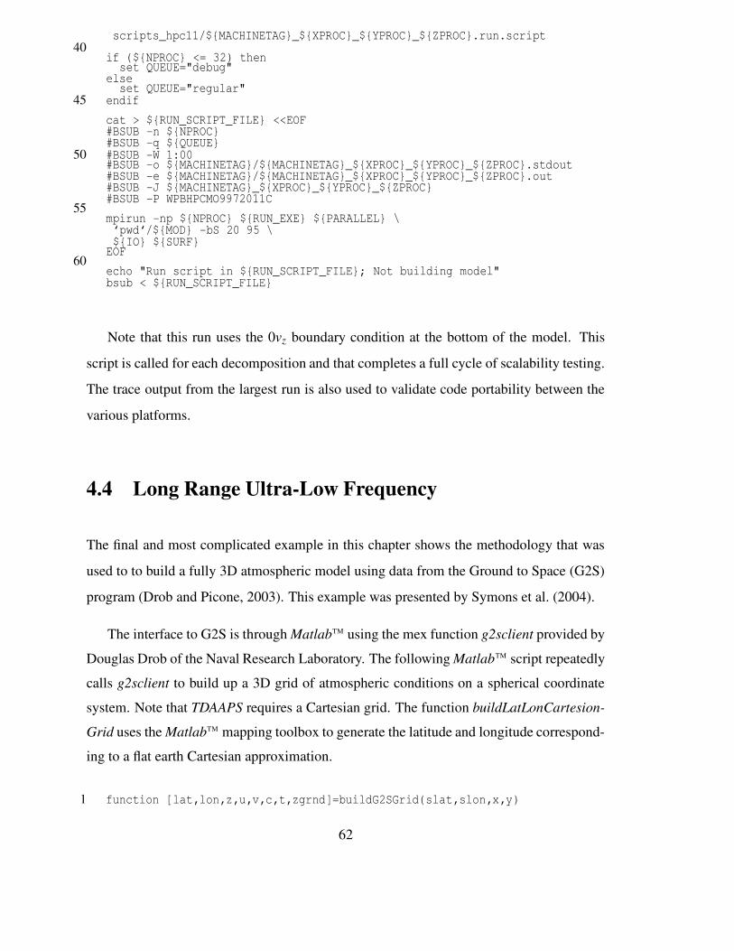
scripts_hpc11/$MACHINETAG_$XPROC_$YPROC_$ZPROC.run.script40
if ($NPROC <= 32) thenset QUEUE="debug"
elseset QUEUE="regular"
45 endifcat > $RUN_SCRIPT_FILE <<EOF#BSUB -n $NPROC#BSUB -q $QUEUE
50 #BSUB -W 1:00#BSUB -o $MACHINETAG/$MACHINETAG_$XPROC_$YPROC_$ZPROC.stdout#BSUB -e $MACHINETAG/$MACHINETAG_$XPROC_$YPROC_$ZPROC.out#BSUB -J $MACHINETAG_$XPROC_$YPROC_$ZPROC#BSUB -P WPBHPCMO9972011C
55mpirun -np $NPROC $RUN_EXE $PARALLEL \‘pwd‘/$MOD -bS 20 95 \$IO $SURF
EOF60
echo "Run script in $RUN_SCRIPT_FILE; Not building model"bsub < $RUN_SCRIPT_FILE
Note that this run uses the 0vz boundary condition at the bottom of the model. This
script is called for each decomposition and that completes a full cycle of scalability testing.
The trace output from the largest run is also used to validate code portability between the
various platforms.
4.4 Long Range Ultra-Low Frequency
The final and most complicated example in this chapter shows the methodology that was
used to to build a fully 3D atmospheric model using data from the Ground to Space (G2S)
program (Drob and Picone, 2003). This example was presented by Symons et al. (2004).
The interface to G2S is through MatlabTM using the mex function g2sclient provided byDouglas Drob of the Naval Research Laboratory. The following MatlabTM script repeatedlycalls g2sclient to build up a 3D grid of atmospheric conditions on a spherical coordinatesystem. Note that TDAAPS requires a Cartesian grid. The function buildLatLonCartesion-Grid uses the MatlabTM mapping toolbox to generate the latitude and longitude correspond-ing to a flat earth Cartesian approximation.
1 function [lat,lon,z,u,v,c,t,zgrnd]=buildG2SGrid(slat,slon,x,y)
62
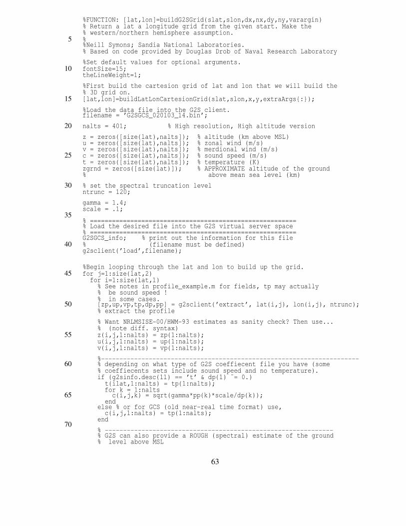
%FUNCTION: [lat,lon]=buildG2SGrid(slat,slon,dx,nx,dy,ny,varargin)% Return a lat a longitude grid from the given start. Make the% western/northern hemisphere assumption.
5 %%Neill Symons; Sandia National Laboratories.% Based on code provided by Douglas Drob of Naval Research Laboratory%Set default values for optional arguments.
10 fontSize=15;theLineWeight=1;%First build the cartesion grid of lat and lon that we will build the% 3D grid on.
15 [lat,lon]=buildLatLonCartesionGrid(slat,slon,x,y,extraArgs:);%Load the data file into the G2S client.filename = ’G2SGCS_020103_14.bin’;
20 nalts = 401; % High resolution, High altitude versionz = zeros([size(lat),nalts]); % altitude (km above MSL)u = zeros([size(lat),nalts]); % zonal wind (m/s)v = zeros([size(lat),nalts]); % merdional wind (m/s)
25 c = zeros([size(lat),nalts]); % sound speed (m/s)t = zeros([size(lat),nalts]); % temperature (K)zgrnd = zeros([size(lat)]); % APPROXIMATE altitude of the ground% above mean sea level (km)
30 % set the spectral truncation levelntrunc = 120;gamma = 1.4;scale = .1;
35% ========================================================% Load the desired file into the G2S virtual server space% ========================================================G2SGCS_info; % print out the information for this file
40 % (filename must be defined)g2sclient(’load’,filename);
%Begin looping through the lat and lon to build up the grid.45 for j=1:size(lat,2)
for i=1:size(lat,1)% See notes in profile_example.m for fields, tp may actually% be sound speed !% in some cases.
50 [zp,up,vp,tp,dp,pp] = g2sclient(’extract’, lat(i,j), lon(i,j), ntrunc);% extract the profile% Want NRLMSISE-00/HWM-93 estimates as sanity check? Then use...% (note diff. syntax)
55 z(i,j,1:nalts) = zp(1:nalts);u(i,j,1:nalts) = up(1:nalts);v(i,j,1:nalts) = vp(1:nalts);%----------------------------------------------------------------------
60 % depending on what type of G2S coeffiecent file you have (some% coeffiecents sets include sound speed and no temperature).if (g2sinfo.desc(11) == ’t’ & dp(1) ˜= 0.)
t(ilat,1:nalts) = tp(1:nalts);for k = 1:nalts
65 c(i,j,k) = sqrt(gamma*pp(k)*scale/dp(k));end
else % or for GCS (old near-real time format) use,c(i,j,1:nalts) = tp(1:nalts);
end70
% --------------------------------------------------------------% G2S can also provide a ROUGH (spectral) estimate of the ground% level above MSL
63
% Note: you may get numbers less than zero due to spectral ringing75 % effects.
zgrnd(i,j) = g2sclient(’zgrnd’);end
end
The next script then takes as input the atmospheric and wind properties read withbuildG2SGrid.m and writes out 3D model and wind NetCDF files.
1 function [c,d,u,v,X,Y,Z]=buildModel(filenameroot,x,y,z,t,varargin)%Set default values for optional arguments.writeModel=1;
5 splitFiles=0;%Check varargin for modifiers to the default arguments.i=1;while i<=length(varargin)
10 currArg=varargini;i=i+1;argType=whos(’currArg’);if ˜strcmp(argType.class,’char’)
error(sprintf(’Optional argument %i, type %s must be char’,...15 i,argType.class));
endswitch lower(currArg)
case ’datafile’20 datafilename=varargini+0;
i=i+1;case ’data’
c=varargini+0;25 d=varargini+1;
u=varargini+2;v=varargini+3;i=i+4;
30 case ’properties’ ’prop’c=varargini+0;d=varargini+1;i=i+2;
35 case ’wind’u=varargini+0;v=varargini+1;i=i+2;
40 otherwiseerror(sprintf(’Unknown option %s’,currArg));
endend
45 %Load or create required variables.if exist(’c’)˜=1 & exist(’d’)˜=1 & exist(’u’)˜=1 & exist(’v’)˜=1
z1=z;if exist(’datafilename’)˜=1
load 101x121v6.mat;50 else
eval(sprintf(’load %s’,datafilename));endz=z1;end
55[X,Y,Z]=meshgrid([0:10:1200],[0:10:1000],[0:0.5:200]);xmin=min(flatten(X));xmax=max(flatten(X));
64
ymin=min(flatten(Y));ymax=max(flatten(Y));60 zmin=min(flatten(Z));zmax=max(flatten(Z));
%Get the model sizes.params.NX=length(x);params.NY=length(y);
65 params.NZ=length(z);params.NT=length(t);fprintf(’Building %ix%ix%i (%.2fM) node model; %i time steps\n’,...
params.NX,params.NY,params.NZ,params.NX*params.NY*params.NZ/1e6,params.NT);70 %Open a file for the wind and a file for the sound speed/density.
if exist(’u’)==1 & exist(’v’)==1windOut=openNetCDF(sprintf(’%s.wind.cdf’,filenameroot),x,y,z,t,’WindVx’ ’WindVy’);
endif exist(’c’)==1 & exist(’d’)==1
75 propOut=openNetCDF(sprintf(’%s.prop.cdf’,filenameroot),x,y,z,t,’vp’ ’rho’);end%Now fill in the values 1 layer at a time.wh=waitbar(0,’null’,...
80 ’Name’,sprintf(’%i Layer Waitbar’,length(z)));for k=1:length(z)
waitbar(k/length(z),wh,sprintf(’Layer %i’,k));[XI,YI,ZI]=meshgrid(x,y,z(k));
85 XI=XI/1000;YI=YI/1000;ZI=ZI/1000;
if exist(’windOut’)==1 | (exist(’windOutVx’)==1 & exist(’windOutVy’)==1)90 %Now make the interpolation for the wind.
windVx=interp3(X,Y,Z,u,XI,YI,ZI,’linear’);windVx(isnan(windVx))=0;windVy=interp3(X,Y,Z,v,XI,YI,ZI,’linear’);
95 windVy(isnan(windVy))=0;windOut’WindVx’(k,:,:)=windVx;windOut’WindVy’(k,:,:)=windVy;
end100
if exist(’propOut’)==1 | (exist(’propOutVp’)==1 & exist(’propOutRho’)==1)%Now make the interpolation for the material properties.vp=interp3(X,Y,Z,c,XI,YI,ZI,’linear’);vp(isnan(vp))=342;
105rho=interp3(X,Y,Z,d,XI,YI,ZI,’linear’);rho=rho*100*100*100/1000; %Convert from g/cmˆ3 to Kg/mˆ3.rho(isnan(rho))=1.2;
110 propOut’vp’(k,:,:)=vp;propOut’rho’(k,:,:)=rho;
endendclose(wh);
115close(windOut);close(propOut);%%%
120 %%%LOCAL FUNCTIONS%%%%%FUNCTION [out]=openNetCDFFile(filename,params)function [out]=openNetCDF(filename,x,y,z,t,vars)
125%Open the file.if exist(’params’)==2 & isfield(params,’noclobber’)==1 & params.noclobber
out=netcdf(filename,’write’);else
65
130 out=netcdf(filename,’clobber’);%Set some global attribute describing how this file was created.out.title=’Staggered Grid Finite-Difference Model Input File’;out.history=’Created with matlab writeSgfdModel.m’;
135 if exist(’params’)==1 & isfield(params,’comment’)out.comment=params.comment;
end%Set the dimensions.
140 out(’numCoord’)=4;out(’NX’)=length(x);out(’NY’)=length(y);out(’NZ’)=length(z);out(’NT’)=length(t);
145%Define and fill the increment variables.out’minima’=ncfloat(’numCoord’);out’minima’(:)=[x(1) y(1) z(1) t(1)];out’increments’=ncfloat(’numCoord’);
150 out’increments’(:)=[x(2)-x(1) y(2)-y(1) z(2)-z(1) t(2)-t(1)];%Define and fill the position variables.out’x’=ncfloat(’NX’);out’x’(:)=x;
155 out’y’=ncfloat(’NY’);out’y’(:)=y;out’z’=ncfloat(’NZ’);out’z’(:)=z;out’time’=ncfloat(’NT’);
160 out’time’(:)=t;endfor i=1:length(vars)
outvarsi=ncfloat(’NZ’,’NY’,’NX’);165 end
The model resulting from this sequence of scripts is quite heterogeneous (Figure 4.4).
A close examination of the results (Figure 4.5) shows the effects of this heterogeneity.
This model is interesting for a number of reasons. First, the finest grid spacing at-
tempted was 500m; with this spacing and the desired range the model was 1001× 801×
403(∼ 323M) nodes. For this fairly large run, the model and wind variables where stored
in four (G2S does not give vz so it was assumed to be 0) individual files each of which was
∼ 1.2Gb in size. Second, this model was successfully run on an older supercomputer (SNL
ASCI Red) with a 20×16×8(2560) processors decomposition. Although no scalability
testing was done with this number of processors, it is significant that such a decomposition
can be successfully run.
66
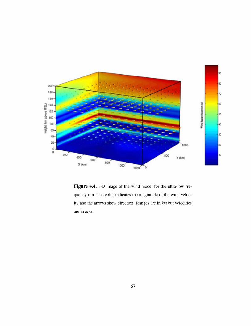
Figure 4.4. 3D image of the wind model for the ultra-low fre-
quency run. The color indicates the magnitude of the wind veloc-
ity and the arrows show direction. Ranges are in km but velocities
are in m/s.
67
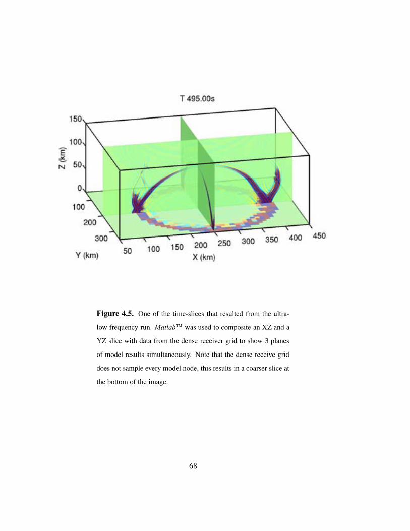
Figure 4.5. One of the time-slices that resulted from the ultra-
low frequency run. MatlabTM was used to composite an XZ and a
YZ slice with data from the dense receiver grid to show 3 planes
of model results simultaneously. Note that the dense receive grid
does not sample every model node, this results in a coarser slice at
the bottom of the image.
68
References
Aldridge, D. F. (2005). Staggered grid finite difference acoustic wave modeling. SAND
Report, in preparation.
Backus, J. W. (1959). The syntax and semantics of the proposed international algebraic
language of the Zurich ACM-GAMM conference. In Proceedings of the International
Conference on Information Processing, pages 125–132.
Bartel, L. C., Symons, N. P., and Aldridge, D. F. (2000). Graded boundary simulation of
air/earth interfaces in finite-difference elastic wave modeling, page 71. Soc. Of Expl.
Geophys., 70th Ann. Internat. Mtg.
Bayliss, A., Jordan, K. E., LeMesurier, B. J., and Turkel, E. (1986). A fourth-order accu-
rate finite-difference scheme for the computation of elastic waves. Bull. Seis. Soc. Am.,
76:1115–1132.
Berenger, J.-P. (1994). A perfectly matched layer for the absorption of electromagnetic
waves. J. Comp. Phys., 114:185–200.
Berengier, M. and Daigle, G. A. (1988). Diffraction of sound above a curved surface having
an impedance discontinuity. J. Acoust. Soc. Am., 84:1055–1060.
Berliner, B. (1990). CVSII: Parallelizing software development. In Winter 1990 USENIX
Conference, Washington D.C.
Cerjan, C., Kosloff, D., Kosloff, R., and Reshef, M. (1985). A nonreflecting boundary-
condition for discrete acoustic and elastic wave-equations. Geophysics, 50:705–708.
69
Collier, S. L., Ostashev, V. E., Wilson, D. K., and Marlin, D. H. (2002). Implementa-
tion of ground boundary conditions in a finite-difference time-domain model of acoustic
wave propagation. In Proceedings of the 2003 Meeting of the MSS Specialty Group on
Battlefield Acoustic and Seismic Sensing, Magnetic and Electric Field Sensors, Laurel,
MD.
Denham, C. R. (2000). MexCDF and NetCDF toolbox for Matlab-5/6.
http://crusty.er.usgs.gov/ cdenham/MexCDF/nc4ml5.html.
Drob, D. . and Picone, J. M. (2003). Global morphology of infrasound propagation. J.
Geophys. Res., 108(D21).
Geist, G. A., Kohl, J. A., and Papadopoulos, P. A. (1996). PVM and MPI: A comparison
of features. Calculateurs Paralleles Vol. 8 No. 2 (1996), 8(2).
Goedecke, G., Ostashev, V. E., Wilson, D. K., and Auvermann, H. J. (2004). Quasi-wavelet
model of von karman spectrum of turbulent velocity flucuations. Bound.-Lay. Meteorol,
112:33–56.
Goedecke, G. H. and Auvermann, H. J. (1997). Acoustic scattering by atmospheric tur-
bules. J. Acoust. Soc. Am., 102(759-771).
Graves, R. W. (1996). Simulating seismic wave propagation in 3D elastic media using
staggered-grid finite differences. Bull. Seis. Soc. Am., 86:1091–1106.
Levander, A. R. (1988). Fourth-order finite-difference P-SV seismograms. Geophysics,
53:1425–1436.
Ostashev, V. E. (1997). Acoustics in Moving Inhomogeneous Media. E&FN SPON, Lon-
don.
Ostashev, V. E., Wilson, D. K., Liu, L., Aldridge, D. F., Symons, N. P., and Marlin, D.
(2005). Equations for finite-difference, time-domain simulation of sound propagation
in moving inhomogeneous media and numerical implementation. J. Acoust. Soc. Am.,
117(2).
70
Rew, R., Davis, G., Emmerson, S., and Davies, H. (1997). NetCDF User’s Guide for C;
Version 3. Unidata Program Center.
Sullivan, P. P., McWilliams, J. C., and Moeng, C.-H. (1996). A grid nesting method for
large-eddy simulation of planetary boundary flows. Bound.-Lay. Meteorol., 80:167–
2002.
Symons, N. and Aldridge, D. (2000). 3-D elastic modeling of salt flank reflections at Bayou
Choctaw Salt Dome, Louisiana. In 70th Annual Internat. Mtg., Soc. Expl. Geophys.,
Expanded Abstracts, page Session: ST P1.6. Soc. Expl. Geophys.
Symons, N. P., Aldridge, D. F., Marlin, D. H., Wilson, D. K., Patton, E. G., Sullivan, P. P.,
Collier, S. L., Ostashev, V. E., and Drob, D. P. (2004). 3d staggered-grid finite-difference
simulation of sound refraction and scattering in moving-media. In Proceedings, 11th
Long Range Sound Propagation Symposium, June 1-3.
Symons, N. P., Aldridge, D. F., Wilson, D. K., Marlin, D., and Ostashev, V. (2003). 3d
finite-difference simulation of acoustic waves in turbulent moving media. J. Acoust.
Soc. Am., 114(4):2440.
Virieux, J. (1986). P-SV wave propagation in heterogeneous media: velocity-stress finite-
difference method. Geophysics, 51:889–901.
Wilson, D. K. (1993). Relaxation-matched modeling of propagation throught porous me-
dia, including fractal pore structure. J. Acoust. Soc. Am., 94:1136–1145.
Wilson, D. K. (1997). Simple, relaxational models for the acoustical properties of porous
media. Appl. Acoust., 50:171–188.
Zwikker, C. and Kosten, C. W. (1949). Sound Absorbing Materials. Elsevier, New York.
71

This page intentionally blank
72
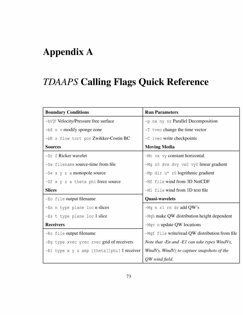
Appendix A
TDAAPS Calling Flags Quick Reference
Boundary Conditions Run Parameters-bV|F Velocity/Pressure free surface -p nx ny nz Parallel Decomposition
-bS n v modify sponge zone -T tvec change the time vector
-bK z flow tort por Zwikker-Costin BC -C ivec write checkpoints
Sources Moving Media-Sr f Ricker wavelet -Mc vx vy constant horizontal
-Sw filename source-time from file -Mg z0 dvx dvy vx0 vy0 linear gradient
-Se x y z a monopole source -Mp dir u* z0 logrithmic gradient
-Sf x y z a theta phi force source -Mf file wind from 3D NetCDF
Slices -M1 file wind from 1D text file
-Eo file output filename Quasi-wavelets-En n type plane loc n slices -Mq n r1 rn dr add QW’s
-Es t type plane loc 1 slice -Mqh make QW distribution height dependent
Receivers -Mqv n update QW locations
-Ro file output filename -Mqf file write/read QW distribution from file
-Rg type xvec yvec zvec grid of receivers Note that -En and -E1 can take types WindVx,
-R1 type x y z amp [theta][phi] 1 receiver WindVy, WindVz to capture snapshots of the
QW wind field.
73

This page intentionally blank
74
Appendix B
Examples from the Beta Test
This appendix consists entirely of a set of examples. TDAAPS was required to meet a set
of specifications for DOD acceptance of the final product. These are the runs that where
performed for the successful Beta Test. The scripts for model generation and running in
the previous examples in this document have been “cleaned up” to remove complications
that result from the use of large models and long run times. The examples in this section
are largely “as run”; as such, they are longer and include details such as building models
that are too large to fit into memory one layer at a time.
B.1 Hill Test
The original Beta Test plan called for a hill to be implemented as a transition over a singlelayer of nodes from the atmospheric conditions (C 342m/s and ρ 1.2Kg/m3) to a hard,dense, rock-like material (C 3500m/s and ρ 1500Kg/m3). We planned to use only a singletransitional layer of density nodes to maintain stability (Bartel et al., 2000). However, oncethe test was underway we determined that “stair-step” diffractions from the surface of thehill were scattering far too much energy into the shadow zone behind the hill. We wereable to fix this effect and obtain an acceptable match to the analytic solution (Berengierand Daigle, 1988) by smoothing the interface. The smoothing was performed by assigning
75
nodes that were within a distance of 2 grid interval or less of the cylinder surface a valuethat was the weighted harmonic average of the air and ground properties. The final gridspacing for this model was 0.25m and the total model was 951× 701× 551(∼ 367M)
nodes. The large size of the model meant that the complete 3D velocity and/or density fieldcould not be stored in memory at one time in MatlabTM. For this reason the following script(build hill model2.m contains two functions for building the velocity and density. If themodel size is small the simple function to build the fields in one step is used; however, ifthe model is large, then the fields are built up one layer a time.
1 function [mName]=build_hill_model(dx,varargin)%% Define the parameters of the model buildif nargin<1
dx=0.50;enddt=2.5e-5*dx;maxT=2.0;standoff=8;
10 offset=50*dx;soffset=100*dx;minUX=100;minX=-minUX-soffset;maxX=minUX+offset;yrange=75+offset;minZ=-soffset;maxZ=100+offset;
20 %% Define the parameters of the cylindrical hill.center=[0 -200];radius=sqrt(center(2)ˆ2+minUXˆ2);%% Build vectors for the axes.x=[minX:dx:maxX];y=[-yrange:dx:yrange];z=[minZ:dx:maxZ];t=[0:dt:maxT];
30NX=length(x);NY=length(y);NZ=length(z);NT=length(t);%% Build vectors for the receiver array and source.re=5;rx=[-minUX+10:5:minUX];ry=0*rx;
40 rz=sqrt((radius+re)ˆ2-rx.ˆ2)+center(2);sl=[-minUX 0 sqrt((radius+re)ˆ2-minUX.ˆ2)+center(2)];sw=monofreq(100,dt,length(t),’dur’,maxT,’plot’);%clear offset soffset minUX minX maxX yrange minZ maxZ;%% Write the basic model.mName=sprintf(’BetaHill2.dx%03i.dt%0g.ft%03i.cdf’,100*dx,dt,100*maxT);fprintf(’Model is %ix%ix%i (%.1fM) nodes; %i time-steps=>\n\t%s\n’,...
50 NX,NY,NZ,NX*NY*NZ/1e6,NT,mName);writeSgfdModel(mName,x,y,z,t,...
’comment’,sprintf(’Version 1.0: dx=%.1f; dt=%5g’,dx,dt),...’history’,textFromFile(’build_hill_model.m’),...’pressurereceivers’,rx,ry,rz,...
76
’pressuresource’,sl,sw);clear re rx ry rz sl sw;out=netcdf(mName,’write’);out.title=’TDAPS Beta Test Hill Model Input File’;
60%% And fill in the variables.if NX*NY*NZ/1e6<25
fprintf(’\tBuilding complete model in 3D\n’);build_model_3D;
elsefprintf(’\tBuilding model 1 layer at a time\n’);build_model_layer_at_a_time;
end70 %% Close the file.
close(out);clear out;clear offset soffset minUX minX maxX yrange minZ maxZ;%% Now make a plot of the variable(s).% plot_model(mName,’vp’,’yflip’,’colorbar’,’horz’,’subplot’,2,1,1);% plot_model(mName,’rho’,’yflip’,’colorbar’,’horz’,’subplot’,2,1,2);if exist(’mNameRho’)==1
80 plot_model(mNameRho,’rho’,’yflip’,’colorbar’,’horz’,’subplot’,2,1,1);plot_model(mNameRho,’rho’,’yflip’,’colorbar’,’horz’,’subplot’,2,2,3,...’yz’,’index’,11);plot_model(mNameRho,’rho’,’yflip’,’colorbar’,’horz’,’subplot’,2,2,4,...
’yz’,’index’,10);else
plot_model(mName,’rho’,’yflip’,’colorbar’,’horz’,’subplot’,2,1,1);plot_model(mName,’rho’,’yflip’,’colorbar’,’horz’,’subplot’,2,2,3,...
’yz’,’index’,11);plot_model(mName,’rho’,’yflip’,’colorbar’,’horz’,’subplot’,2,2,4,...
90 ’yz’,’index’,10);end%% LOCAL FUNCTIONS%%%% function build_model_3D% Build the complete 3D model in one step. This is the easiest way to do it% if the model is not too large to fit into memory all at once.
100 function build_model_3D[Y,Z,X]=meshgrid(y,z,x);%clear Y;D=sqrt(X.ˆ2+(Z-center(2)).ˆ2);%clear X Z;%% Define a variable for vp and fill it in.out’vp’=ncfloat(’NZ’,’NY’,’NX’);vp=342*ones(NZ,NY,NX);vp(D<=radius &...
110 X>(minX+standoff*dx) & X<(maxX-standoff*dx) & ...Y>(-yrange+standoff*dx) & Y<(yrange-standoff*dx) &...Z>(minZ+standoff*dx))=3500;
dx2=sqrt(2)*dx*2;for i=standoff+2:NX-standoff-2
for j=standoff+2:NY-standoff-2for k=standoff+2:NZ-standoff-2
if abs(radius-D(k,j,i))<dx2% This is within one node of the surface.
120 if D(k,j,i)>radius%This is the air side.dA=(D(k,j,i)-radius)/dx2/2;%vp(k,j,i)=1/((1-dA)/342+(dA)/3500);vp(k,j,i)=1/((0.5+dA)/342+(0.5-dA)/3500);
else
77
%This is the rock side or the exact middle.dR=(radius-D(k,j,i))/dx2/2;%vp(k,j,i)=1/((dR)/342+(1-dR)/3500);vp(k,j,i)=1/((0.5-dR)/342+(0.5+dR)/3500);
130 endend
endend
end% imagesc(x,z,squeeze(vp(:,1,:)));% axis image;% colorbar(’horz’);% set(gca,’YDir’,’normal’);
140 out’vp’(:,:,:)=vp;%% Determine a 1st order polynomial to fit the vp vs. rho.p=polyfit([342 3500],[1.2 2000],1);rho=polyval(p,vp);%% Define a variable for rho and fill it in.out’rho’=ncfloat(’NZ’,’NY’,’NX’);rho=1.2*ones(NZ,NY,NX);rho(vp>1000)=2000;
150 for i=1:NXfor j=1:NYfor k=1:NZ-1
if rho(k,j,i)>1000modify=0;for ii=max(1,i-1):min(NX,i+1)for jj=max(1,j-1):min(NY,j+1)
for kk=max(1,k-1):min(NZ,k+1)if vp(kk,jj,ii)<500
modify=1;160 end
endend
endif modifyrho(k,j,i)=100;
endend
endend
170 endout’rho’(:,:,:)=rho;clear rho vp;clear X Y Z;
end % function build_model_3D
%% function build_model_layer_at_a_time% Build the 3D model one layer at a time. This is more complicated but is% required if the model is too large to fit into memory at one time.
180 function build_model_layer_at_a_timeif NX*NY*NZ/1e6>0.250
fprintf(’Creating seperate files for Vp and Rho\n’);mNameVp=sprintf(’BetaHill2.dx%03i.dt%0g.ft%03i_vp.cdf’,...100*dx,dt,100*maxT);
mNameRho=sprintf(’BetaHill2.dx%03i.dt%0g.ft%03i_rho.cdf’,...100*dx,dt,100*maxT);
writeSgfdModel(mNameVp,x,y,z,t);outVp=netcdf(mNameVp,’write’);writeSgfdModel(mNameRho,x,y,z,t);
190 outRho=netcdf(mNameRho,’write’);else
outVp=out;outRho=out;
end%% Make the grid for one layer only.[X,Y]=meshgrid(x,y);
78
%% Define and fill both variables at the same time.200 outVp’vp’=ncfloat(’NZ’,’NY’,’NX’);
vp=342*ones(3,NY,NX);outVp’vp’(1,:,:)=vp(1,:,:);outVp’vp’(end,:,:)=vp(1,:,:);outRho’rho’=ncfloat(’NZ’,’NY’,’NX’);rho=1.2*ones(3,NY,NX);outRho’rho’(1,:,:)=rho(1,:,:);outRho’rho’(end,:,:)=rho(1,:,:);
210 dx2=sqrt(2)*dx*2;p=polyfit([342 3500],[1.2 2000],1);wh=waitbar(0,’Layer 1’,’Name’,sprintf(’%i Layers’,NZ));for k=2:length(z)-1
waitbar(k/NZ,wh,sprintf(’Layer %i’,k));% Generate the current distances.D(1,:,:)=sqrt(X.ˆ2+(z(k-1)-center(2)).ˆ2);D(2,:,:)=sqrt(X.ˆ2+(z(k)-center(2)).ˆ2);D(3,:,:)=sqrt(X.ˆ2+(z(k+1)-center(2)).ˆ2);
220%Shift the layers down by one.vp(1,:,:)=vp(2,:,:);vp(2,:,:)=vp(3,:,:);vp(3,:,:)=342*ones(NY,NX);rho(1,:,:)=rho(2,:,:);rho(2,:,:)=rho(3,:,:);rho(3,:,:)=1.2*ones(NY,NX);if k>standoffvp(3,...
230 squeeze(D(3,:,:)<=radius) &...X>(minX+standoff*dx) & X<(maxX-standoff*dx) & ...Y>(-yrange+standoff*dx) & Y<(yrange-standoff*dx))=3500;
for i=standoff+2:NX-standoff-2for j=standoff+2:NY-standoff-2
if abs(radius-D(3,j,i))<dx2% This is within one node of the surface.if D(3,j,i)>radius
dA=(D(3,j,i)-radius)/dx2/2;vp(3,j,i)=1/((0.5+dA)/342+(0.5-dA)/3500);
240 elsedR=(radius-D(3,j,i))/dx2/2;vp(3,j,i)=1/((0.5-dR)/342+(0.5+dR)/3500);
endend
endend
endoutVp’vp’(k,:,:)=vp(2,:,:);
250 rho(3,:,:)=polyval(p,vp(3,:,:));for i=1:NXfor j=1:NY
if rho(2,j,i)>100modify=0;for ii=max(1,i-1):min(NX,i+1)for jj=max(1,j-1):min(NY,j+1)
for kk=1:3if vp(kk,jj,ii)<1000
modify=1;260 end
endend
endif modifyrho(2,j,i)=100;
endend
endend
270 outRho’rho’(k,:,:)=rho(2,:,:);
79
endclose(wh);clear D k vp rho;clear X Y;if exist(’mNameVp’)==1
close(outVp);close(outRho);
end280 end % function build_model_layer_at_a_time
%% END of fileend
A cross section of the acoustic sound speed and density through the model that resultsfrom a call to build hill model2(0.25) is shown in Figure B.1. Since this model con-tains a large range of sound speeds (342m/s in the air and 3500m/s in the ground) theboundary conditions were somewhat problematic. After some experimentation we deter-mined that the attenuative layer (Section 2.5) needed to taper to a value that was very closeto unity (0.998). This is because the time-step was small (determined by the CFL ratiousing the high sound speed in the ground) and the waves in the air moved only a very smalldistance in a single time-step. If “normal” values of the attenuation were used the energywas attenuated too quickly and the result was a reflection from the start of the zone. The jobwas run with a 7× 4× 3(84) processors decomposition on the ARL John Von-Neumann(JVN) cluster. This is a Linux Networx Evolocity II using 3.6GHz Intel Xeon EM64Tprocessors. The total run time on the 85 processors was 32hr. Note that TDAAPS hasupdating schemes for both fixed and moving-media acoustic propagation. When no windis specified (as is the case here) the much faster fixed media updating is used. The fixedmedia updates require 45 floating point operations (FPO)/grid-point/time-step, while themoving media updates require 300 FPO/grid-point/time-step. The run was performed withthe following script (BH2M100.script):
1 #!/bin/tcsh#BSUB -n 85#BSUB -m jvn#BSUB -a mpich_gm#BSUB -q standard#BSUB -P HPCMO9972011C#BSUB -W 60:00#BSUB -o BH2M100.stdout
10 #BSUB -e BH2M100.stderr#BSUB -J BH2M100module load lsf compiler/intel8.1 mpi/mpich-gm-1.2.6..14ampirun.lsf -np 85 \/home/others/npsymon/curr/bin/2_4_21-286-login_lnxi_0_i686/TDAAPS -p 7 4 3 \-Ro trace.BH2M100.cdf -Eo slice.BH2M100.cdf \
80
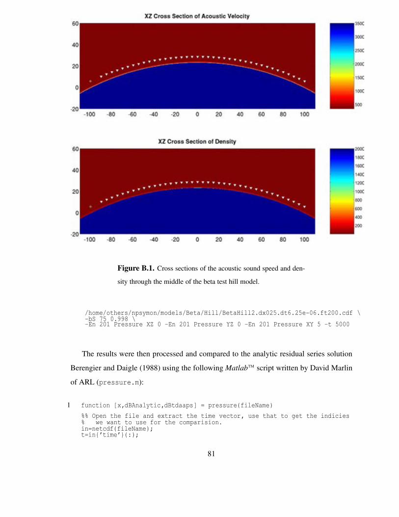
Figure B.1. Cross sections of the acoustic sound speed and den-
sity through the middle of the beta test hill model.
/home/others/npsymon/models/Beta/Hill/BetaHill2.dx025.dt6.25e-06.ft200.cdf \-bS 75 0.998 \-En 201 Pressure XZ 0 -En 201 Pressure YZ 0 -En 201 Pressure XY 5 -t 5000
The results were then processed and compared to the analytic residual series solution
Berengier and Daigle (1988) using the following MatlabTM script written by David Marlin
of ARL (pressure.m):
1 function [x,dBAnalytic,dBtdaaps] = pressure(fileName)%% Open the file and extract the time vector, use that to get the indicies% we want to use for the comparision.in=netcdf(fileName);t=in’time’(:);
81
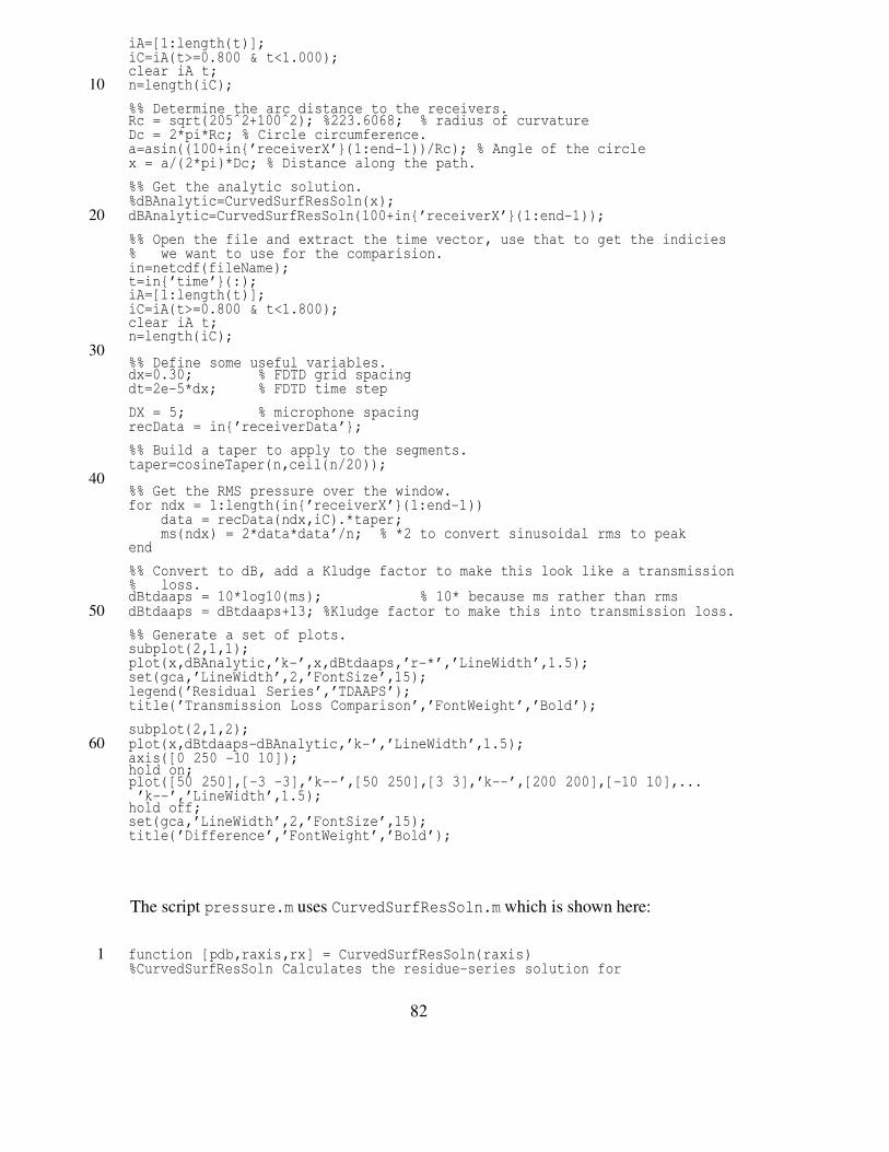
iA=[1:length(t)];iC=iA(t>=0.800 & t<1.000);clear iA t;
10 n=length(iC);%% Determine the arc distance to the receivers.Rc = sqrt(205ˆ2+100ˆ2); %223.6068; % radius of curvatureDc = 2*pi*Rc; % Circle circumference.a=asin((100+in’receiverX’(1:end-1))/Rc); % Angle of the circlex = a/(2*pi)*Dc; % Distance along the path.%% Get the analytic solution.%dBAnalytic=CurvedSurfResSoln(x);
20 dBAnalytic=CurvedSurfResSoln(100+in’receiverX’(1:end-1));%% Open the file and extract the time vector, use that to get the indicies% we want to use for the comparision.in=netcdf(fileName);t=in’time’(:);iA=[1:length(t)];iC=iA(t>=0.800 & t<1.800);clear iA t;n=length(iC);
30%% Define some useful variables.dx=0.30; % FDTD grid spacingdt=2e-5*dx; % FDTD time stepDX = 5; % microphone spacingrecData = in’receiverData’;%% Build a taper to apply to the segments.taper=cosineTaper(n,ceil(n/20));
40%% Get the RMS pressure over the window.for ndx = 1:length(in’receiverX’(1:end-1))
data = recData(ndx,iC).*taper;ms(ndx) = 2*data*data’/n; % *2 to convert sinusoidal rms to peak
end%% Convert to dB, add a Kludge factor to make this look like a transmission% loss.dBtdaaps = 10*log10(ms); % 10* because ms rather than rms
50 dBtdaaps = dBtdaaps+13; %Kludge factor to make this into transmission loss.%% Generate a set of plots.subplot(2,1,1);plot(x,dBAnalytic,’k-’,x,dBtdaaps,’r-*’,’LineWidth’,1.5);set(gca,’LineWidth’,2,’FontSize’,15);legend(’Residual Series’,’TDAAPS’);title(’Transmission Loss Comparison’,’FontWeight’,’Bold’);subplot(2,1,2);
60 plot(x,dBtdaaps-dBAnalytic,’k-’,’LineWidth’,1.5);axis([0 250 -10 10]);hold on;plot([50 250],[-3 -3],’k--’,[50 250],[3 3],’k--’,[200 200],[-10 10],...’k--’,’LineWidth’,1.5);
hold off;set(gca,’LineWidth’,2,’FontSize’,15);title(’Difference’,’FontWeight’,’Bold’);
The script pressure.m uses CurvedSurfResSoln.m which is shown here:
1 function [pdb,raxis,rx] = CurvedSurfResSoln(raxis)%CurvedSurfResSoln Calculates the residue-series solution for
82
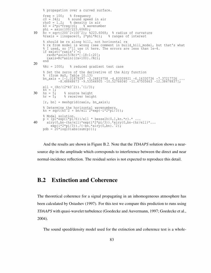
% propagation over a curved surface.freq = 100; % frequencyc0 = 342; % sound speed in airrho0 = 1.2; % density in airk0 = 2*pi*freq/c0; % wavenumberphi = asin(100/223.6068);
10 Rc = sqrt(200ˆ2+100ˆ2); %223.6068; % radius of curvature%raxis = linspace(0, 2*phi*Rc); % ranges of interest% should be rs along hill, not horizontal rx% rx from model is wrong (see comment in build_hill_model, but that’s what% I used, so I’ll use it here. The errors are less than 1e-4.if exist(’raxis’)˜=1
rx=Rc*asin(5/Rc)*[-18:1:20];raxis=Rc*asin((rx+100)./Rc);
end20
%Rc = 1000; % reduced gradient test case% Set the zeros of the derivative of the Airy function% (from A&S, Table 10.13)bn_axis = [-1.01879297 -3.24819758 -4.82009921 -6.16330736 -7.37217726 ...
-8.48848673 -9.53544905 -10.52766040 -11.47505663 -12.38478837];ell = (Rc/(2*k0ˆ2)).ˆ(1/3);kn = 1;
30 hs = 5; % source heighthr = 5; % receiver height[r, bn] = meshgrid(raxis, bn_axis);% Determine the horizontal wavenumbers.kn = sqrt(k0ˆ2 + bn/ellˆ2*exp(-i*2*pi/3));% Modal solution.p = (pi*exp(i*pi/6))/ell * besselh(0,1,kn.*r).* ...
40 airy(0,bn-(hs/ell)*exp(i*2*pi/3)).*airy(0,bn-(hr/ell)*...exp(i*2*pi/3))./(-bn.*airy(0,bn).ˆ2);
pdb = 20*log10(abs(sum(p)));
And the results are shown in Figure B.2. Note that the TDAAPS solution shows a near-
source dip in the amplitude which corresponds to interference between the direct and near
normal-incidence reflection. The residual series is not expected to reproduce this detail.
B.2 Extinction and Coherence
The theoretical coherence for a signal propagating in an inhomogeneous atmosphere has
been calculated by Ostashev (1997). For this test we compare this prediction to runs using
TDAAPS with quasi-wavelet turbulence (Goedecke and Auvermann, 1997; Goedecke et al.,
2004).
The sound speed/density model used for the extinction and coherence test is a whole-
83
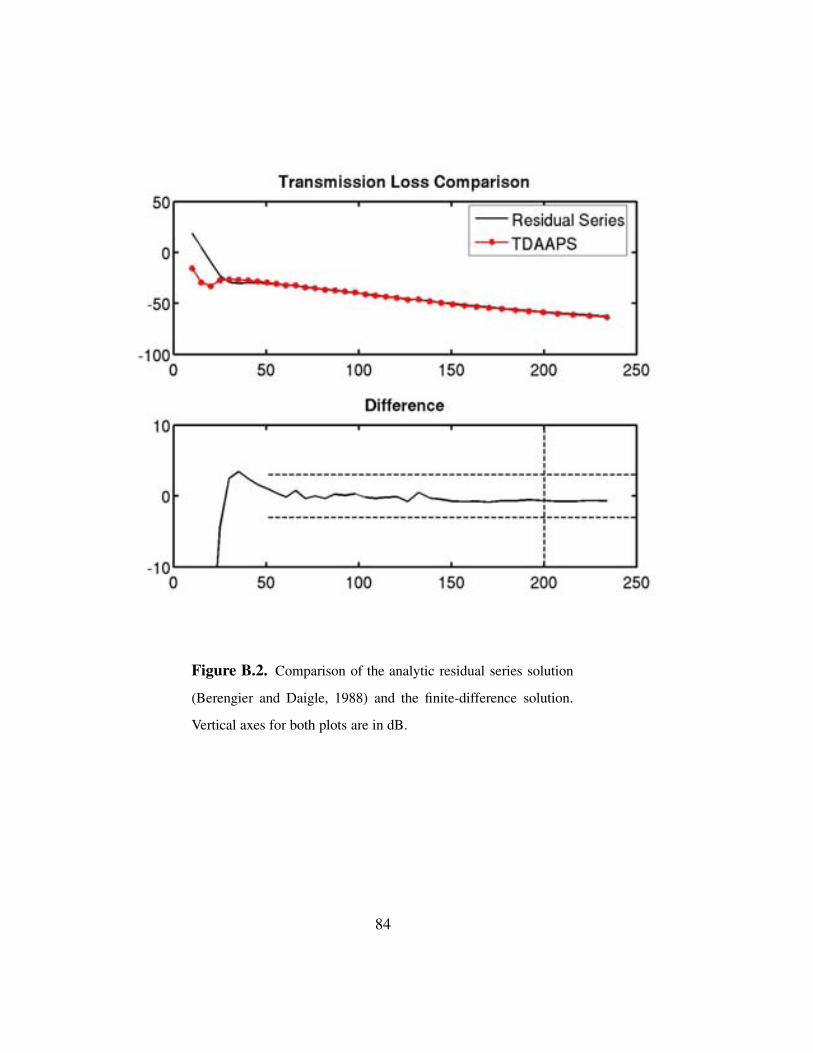
Figure B.2. Comparison of the analytic residual series solution
(Berengier and Daigle, 1988) and the finite-difference solution.
Vertical axes for both plots are in dB.
84
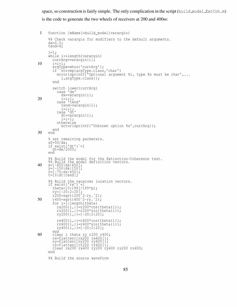
space, so construction is fairly simple. The only complication in the script (build model ExtCoh.m)is the code to generate the two wheels of receivers at 200 and 400m:
1 function [mName]=build_model(varargin)%% Check varargin for modifiers to the default arguments.dx=0.5;tend=4;i=1;while i<=length(varargin)
currArg=varargini;10 i=i+1;
argType=whos(’currArg’);if ˜strcmp(argType.class,’char’)
error(sprintf(’Optional argument %i, type %s must be char’,...i,argType.class));
endswitch lower(currArg)
case ’dx’dx=varargini;
20 i=i+1;case ’tend’
tend=varargini;i=i+1;
case ’dt’dt=varargini;i=i+1;
otherwiseerror(sprintf(’Unknown option %s’,currArg));
end30 end
% set remaining parmeters.sf=50/dx;if exist(’dt’)˜=1
dt=dx/2000;end%% Build the model for the Extinction-Coherence test.%% Build the model definition vectors.
40 x=[-450:dx:450];y=[-150:dx:150];z=[-75:dx:450];t=[0:dt:tend];%% Build the receiver location vectors.if exist(’rx’)˜=1
theta=[0:199]/199*pi;ry=[-20:2:20];r200=sqrt(200ˆ2-ry.ˆ2);
50 r400=sqrt(400ˆ2-ry.ˆ2);for i=1:length(theta)
rx200(i,:)=r200*cos(theta(i));rz200(i,:)=r200*sin(theta(i));ry200(i,:)=[-20:2:20];rx400(i,:)=r400*cos(theta(i));rz400(i,:)=r400*sin(theta(i));ry400(i,:)=[-20:2:20];
end60 clear i theta ry r200 r400;
rx=flatten([rx200 rx400]);ry=flatten([ry200 ry400]);rz=flatten([rz200 rz400]);clear rx200 rx400 ry200 ry400 rz200 rz400;
end%% Build the source waveform
85
sWF=monofreq(sf,dt,length(t),’dur’,t(end),’ts’,0.1,’te’,0.1,’plot’);drawnow;
70%% Create the model.mName=sprintf(’extinctionModel.dx%02.0f.ft%.0f.cdf’,10*dx,10*t(end));sliceT=[1:101]/101*(t(end)-t(1))+t(1);writeSgfdModel(mName,x,y,z,t,...
’comment’,...’Built with: ˜/models/CHSSI/Beta/ExtinctionCoherence/build_model.m’,...’history’,textFromFile(’build_model.m’),...’1D’,342,0,1.2,...’PressureReceivers’,rx,ry,rz,...
80 ’explosion’,[0 0 0],sWF,...’slice’,’xzPressure’,sliceT,0);
The model built by this script is 1801×601×1051(∼ 1137M) nodes.
For this test we performed two separate runs of TDAAPS. The runs used a 8× 3×5(120) processors decomposition. The runs took 65hr on the ARL JVN machine. Both ofthese runs used the AF:arg file syntax to reduce the length of the actual calls to TDAAPSwithin the scripts. The first script and argument file are for no turbulence:
1 #!/bin/tcsh#BSUB -n 121#BSUB -m jvn
5 #BSUB -a mpich_gm#BSUB -q standard#BSUB -P HPCMO9972011C#BSUB -W 75:00#BSUB -o ExtCoh_fixed.stdout
10 #BSUB -e ExtCoh_fixed.stderr#BSUB -J ExtCoh_fixedmodule load lsf compiler/intel8.1 mpi/mpich-gm-1.2.6..14ampirun.lsf -np 121 \
15 /home/others/npsymon/curr/bin/2_4_21-286-login_lnxi_0_i686/TDAAPS -p 8 3 5 \AF:args.run_05_fixed
with the argument file:
1 /home/others/npsymon/models/Beta/ExtinctionCoherence/extinctionModel.cdf-Mc 0 0 -bS 50 90-t 1000-Ro
5 /home/others/npsymon/models/Beta/ExtinctionCoherence/trace.dx05.fixed.cdf-Eo/home/others/npsymon/models/Beta/ExtinctionCoherence/slice.dx05.fixed.cdf
And the second with quasi-wavelet turbulence:
1 #!/bin/tcsh
86
#BSUB -n 121#BSUB -m jvn
5 #BSUB -a mpich_gm#BSUB -q standard#BSUB -P HPCMO9972011C#BSUB -W 75:00#BSUB -o ExtCoh_QW.stdout
10 #BSUB -e ExtCoh_QW.stderr#BSUB -J ExtCoh_QWmodule load lsf compiler/intel8.1 mpi/mpich-gm-1.2.6..14ampirun.lsf -np 121 \
15 /home/others/npsymon/curr/bin/2_4_21-286-login_lnxi_0_i686/TDAAPS -p 8 3 5 \AF:args.run_05_QW
with the argument file:
1 /home/others/npsymon/models/Beta/ExtinctionCoherence/extinctionModel.cdf-Mc 0 0 -bS 50 90-Mq auto 32 2 1-t 1000
5 -Ro/home/others/npsymon/models/Beta/ExtinctionCoherence/trace.dx05.QW01.cdf-Eo/home/others/npsymon/models/Beta/ExtinctionCoherence/slice.dx05.QW01.cdf
The data resulting from the two runs of TDAAPS was processed using the followingscript CoherTestBetaNPS.mmodified from an initial version provided by D. Keith Wilson:
1 %% Set some basic parameters.LoadFile = 0; % Set to 1 to load previously calculated data from file; 0% to calculate then save to file.FileName = ’QWScatData’; % filename for loading or saving
5% Graphics parameters.linewidth = 2;fontsize = 14;
10 % Set number of receivers.Ndist = 2; % number of distancesNelem = 21; % number of elements in each arrayNarray = 200; % number of arraysNrcv = Narray*Nelem*Ndist;
15% Open the file without turbulence (QWs).inF = netcdf(’../trace.dx05.fixed.cdf’, ’nowrite’);% Open the file with turbulence (QWs).
20 inQ = netcdf(’../trace.dx05.QW01.cdf’, ’nowrite’);disp(’Loaded NetCDF files.’)% Load the sample times.t = inF’time’(:);
25 dt = t(2) - t(1); % time stepNt = length(t); % number of time stepsIproc = [round(0.4*Nt):Nt]; % indices to process (loads last 6/10 of% signals)clear Iall;
30nSamplesAdj = length(Iproc); % number of samples retained in Hilbert% xfrm
87
nEdgeRem = 800; % number of samples to remove at edgestWin = t(Iproc);
35 tWin = tWin(nEdgeRem+1:end-nEdgeRem);finalLen = 2ˆ(nextpow2(length(tWin))-1);tWin = tWin(1:finalLen) - tWin(1); % time axis for processed datafreq = 100; % acoustic frequency
40 % Loop through files, finding phase and amplitude for each sample.WavePhasor = zeros(Nrcv, 1); % wave phasor for propagation thru turb,% adjusted by reference phasor (wo/turb)wh=waitbar(0,’Processing 00001’,’Name’,sprintf(’%i Receivers’,Nrcv));for m = 1:Nrcv;
45 %disp([’Processing receiver ’ int2str(m) ’ of ’ int2str(Nrcv) ’.’])waitbar(m/Nrcv,wh,sprintf(’Processing %05i’,m));DataF = inF’receiverData’(m,Iproc);DataQ = inQ’receiverData’(m,Iproc);
50 % Window the data with a Tukey window to mitigate end effects. The% first and last 0.1 s are windowed.% 0.2 = duration of windowed region (s), 2.4 = total duration of% processed signal (s). Then calculate Hilbert transform.XfrmDataF = hilbert(tukeywin(nSamplesAdj,0.2/2.4).*DataF’);
55 XfrmDataQ = hilbert(tukeywin(nSamplesAdj,0.2/2.4).*DataQ’);% Take the ratio to find complex phasor time series.WavePhasorTime = XfrmDataQ./XfrmDataF;
60 % Remove first and last 0.2 s (= 800 samples) to avoid edge effects,% take mean.WavePhasor(m) = mean(WavePhasorTime(nEdgeRem+[1:finalLen]));
endtry
65 close wh;catchendsave(FileName, ’WavePhasor’);
70%% Reformat the data.WavePhasor = reshape(WavePhasor, Narray, Nelem, Ndist);%% Plot sample phasor data at 200 m.
75 figure(1)h = plot(reshape(WavePhasor(:,:,1),Narray*Nelem,1), ’.k’);set(h, ’markersize’, 5)hold onazi = linspace(0, 2*pi);
80 h = plot(cos(azi), sin(azi), ’k--’);set(h, ’linewid’, linewidth)axis(’equal’)xlim([-4 4])ylim([-4 4])
85 hold offxlabel(’Real signal (norm)’, ’fontsize’, fontsize)ylabel(’Imag. signal (norm)’, ’fontsize’, fontsize)set(gca, ’fontsize’, fontsize, ’linewid’, linewidth)
90 %% Plot sample phasor data at 400 m.figure(2)h = plot(reshape(WavePhasor(:,:,2),Narray*Nelem,1), ’.k’);set(h, ’markersize’, 5)hold on
95 azi = linspace(0, 2*pi);h = plot(cos(azi), sin(azi), ’k--’);set(h, ’linewid’, linewidth)axis(’equal’)xlim([-4 4])
100 ylim([-4 4])hold offxlabel(’Real signal (norm)’, ’fontsize’, fontsize)
88
ylabel(’Imag. signal (norm)’, ’fontsize’, fontsize)set(gca, ’fontsize’, fontsize, ’linewid’, linewidth)
105%% Calculate the mean data.MeanEnergy200 = mean(abs(reshape(WavePhasor(:,:,1),Narray*Nelem,1)).ˆ2);MeanEnergy400 = mean(abs(reshape(WavePhasor(:,:,2),Narray*Nelem,1)).ˆ2);Mean200 = mean(reshape(WavePhasor(:,:,1),Narray*Nelem,1))/...
110 sqrt(MeanEnergy200);Mean400 = mean(reshape(WavePhasor(:,:,2),Narray*Nelem,1))/...
sqrt(MeanEnergy400);gammaSim200 = -log(abs(Mean200))/200;
115 gammaSim400 = -log(abs(Mean400))/400;% gammaSim200 = -log(real(Mean200))/200;% gammaSim400 = -log(real(Mean400))/400;% Calcualte the coherence data.
120 SecondMom200 = zeros(Nelem, Nelem);SecondMom400 = zeros(Nelem, Nelem);for m = 1:Nelem,
for n = 1:Nelem,SecondMom200(m,n) = (WavePhasor(:,m,1)’*WavePhasor(:,n,1))/Narray;
125 SecondMom400(m,n) = (WavePhasor(:,m,2)’*WavePhasor(:,n,2))/Narray;end
endry = [-20:2:20];
130 ry_diff = ry’*ones(1,Nelem) - ones(Nelem,1)*ry;rsep = [0:2:40]; %[0:2:20];%% Find common spacings between elements.Coher200 = zeros(length(rsep),1);
135 Coher400 = zeros(length(rsep),1);alphaSim200 = zeros(length(rsep),1);alphaSim400 = zeros(length(rsep),1);for m = 1:length(rsep),
I = find(ry_diff == rsep(m));140 Coher200(m) = mean(SecondMom200(I))/MeanEnergy200;
alphaSim200(m) = -log(abs(Coher200(m)))/200;Coher400(m) = mean(SecondMom400(I))/MeanEnergy400;alphaSim400(m) = -log(abs(Coher400(m)))/400;
end145
%% Do calculations at 200mload CoherPred200CorrgammaTheory200 = gammac;alphaTheory200 = alphac;
150fh=figure(3);set(fh,’Name’,’Errors at 200m’);plot(raxis, exp(-alphaTheory200*200), rsep, real(Coher200), ’go’, ...
rsep, imag(Coher200), ’co’)155 % hold on
% plot(rsep, exp(-2*gammaTheory200*200)*ones(size(I)), ’b--’)% hold offxlabel(’Sensor separation (m)’)ylabel(’Coherence’)
160 ylim([-0.2 1.02])disp([’Error in gamma (%) at 200 m: ’, ...
num2str((gammaSim200-gammaTheory200)/gammaTheory200*100)])disp([’Error in alpha (%) for 10-m sep at 200 m: ’, ...
165 num2str((alphaSim200(6)-alphaTheory200(11))/...alphaTheory200(11)*100)])
% This was giving a divide by zero error as originally written. The zero% was the first element of the theory.%alphaErr200 = (alphaSim200-alphaTheory200(1:2:end))./...
170 alphaTheory200(1:2:end)*100;alphaErr200 = (alphaSim200(2:end)-alphaTheory200(3:2:end))./...
alphaTheory200(3:2:end)*100;
89
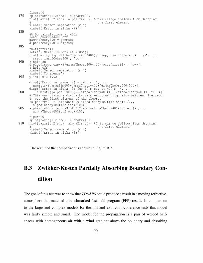
figure(4)175 %plot(raxis(1:2:end), alphaErr200)
plot(raxis(3:2:end), alphaErr200); %This change follows from dropping% the first element.xlabel(’Sensor separation (m)’)ylabel(’Error in alpha (%)’)
180%% Do calculations at 400mload CoherPred400CorrgammaTheory400 = gammac;alphaTheory400 = alphac;
185fh=figure(5);set(fh,’Name’,’Errors at 400m’);plot(raxis, exp(-alphaTheory400*400), rsep, real(Coher400), ’go’, ...
rsep, imag(Coher400), ’co’)190 % hold on
% plot(rsep, exp(-2*gammaTheory400*400)*ones(size(I)), ’b--’)% hold offxlabel(’Sensor separation (m)’)ylabel(’Coherence’)
195 ylim([-0.2 1.02])disp([’Error in gamma (%) at 400 m: ’, ...
num2str((gammaSim400-gammaTheory400)/gammaTheory400*100)])disp([’Error in alpha (%) for 10-m sep at 400 m: ’, ...
200 num2str((alphaSim400(6)-alphaTheory400(11))/alphaTheory400(11)*100)])% This was giving a divide by zero error as originally written. The zero% was the first element of the theory.%alphaErr400 = (alphaSim400-alphaTheory400(1:2:end))./...
alphaTheory400(1:2:end)*100;205 alphaErr400 = (alphaSim400(2:end)-alphaTheory400(3:2:end))./...
alphaTheory400(3:2:end)*100;figure(6)%plot(raxis(1:2:end), alphaErr400)
210 plot(raxis(3:2:end), alphaErr400); %This change follows from dropping% the first element.xlabel(’Sensor separation (m)’)ylabel(’Error in alpha (%)’)
The result of the comparison is shown in Figure B.3.
B.3 Zwikker-Kosten Partially Absorbing Boundary Con-
dition
The goal of this test was to show that TDAAPS could produce a result in a moving refractive-atmosphere that matched a benchmarked fast-field program (FFP) result. In comparisonto the large and complex models for the hill and extinction-coherence tests this modelwas fairly simple and small. The model for the propagation is a pair of welded half-spaces with homogeneous air with a wind gradient above the boundary and absorbing
90
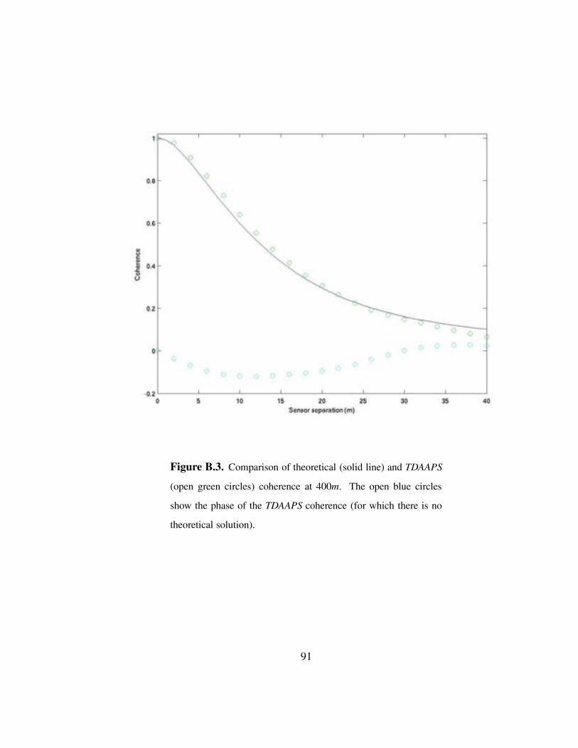
Figure B.3. Comparison of theoretical (solid line) and TDAAPS
(open green circles) coherence at 400m. The open blue circles
show the phase of the TDAAPS coherence (for which there is no
theoretical solution).
91
ground (Zwikker and Kosten, 1949) below the boundary. The input model for TDAAPSis a 551× 401× 281(∼ 62M) nodes whole space. The model was easily created on theUNIX command line with buildSgfdModel:
1 buildSgfdModel acoustic -I \-x -50:0.5:225 -y -100:0.5:100 -z -40:0.5:100 -t 0:0.00025:1.000 \-ml 1 342 1.2 -En 101 Pressure XZ 0 \-Rg Pressure 0:1:200 0:0 1:1 \
5 -Sw mf100\_1.txt -Se 0 0 5 1 model.benchmark2.cdf
The run was performed with a 5× 4× 2(40) processors decomposition on JVN withthe following script:
1 #!/bin/tcsh#BSUB -n 41#BSUB -m jvn
5 #BSUB -a mpich_gm#BSUB -q standard#BSUB -P HPCMO9972011C#BSUB -W 10:00#BSUB -o zkSnowMM.stdout
10 #BSUB -e zkSnowMM.stderr#BSUB -J zkSnowMMmodule load lsf compiler/intel8.1 mpi/mpich-gm-1.2.6..14ampirun.lsf -np 41 \
15 /home/others/npsymon/curr/bin/2_4_21-286-login_lnxi_0_i686/TDAAPS -p 5 4 2 \/home/others/npsymon/models/Beta/ZK/model.benchmarkZK2.cdf \-Mg 0 0.1 0 -bK 0 3000 1.8 0.8 -bS 40 95 \-Eo slice.ZkSnowMM2.cdf -Ro trace.ZkSnowMM2.cdf
This run took less than 1hr. The ZK parameters are: 0m for the interface location, 3000
flow resistivity, 0.8 for the porosity, and 1.3 for the tortuosity. The results of the FFP and
TDAAPS solutions are shown in Figure B.4. The match is excellent except in the near-field.
The FFP is a far-field solution that does not include near-field terms.
92
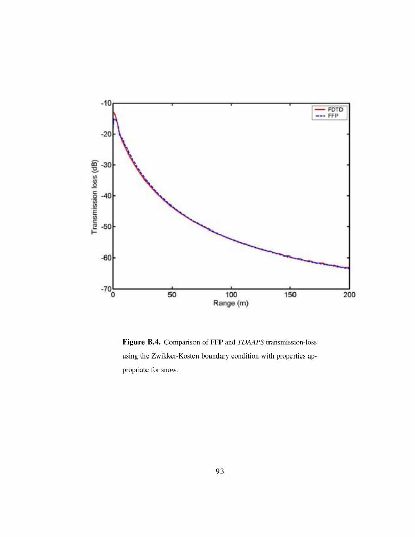
Figure B.4. Comparison of FFP and TDAAPS transmission-loss
using the Zwikker-Kosten boundary condition with properties ap-
propriate for snow.
93

This page intentionally blank
94
Appendix C
Large Eddy Simulation (LES) Example
This appendix is an example of using TDAAPS to propagate sound through a realization of
the large-eddy Simulation (LES) atmospheric model code (Sullivan et al., 1996). This result
was presented in Symons et al. (2004). This example uses an unstable atmospheric case
(mixture of shear and buoyancy influence on the flow), generated by the NCAR LES model.
This LES simulation was run for ug = 5m/s, zi/LMO = −6, and Qs = 0.025mK/s, where
ug is the geostrophic wind, zi is the boundary layer depth, LMO is the Monin-Obukhov
length, and Qs is the surface heat flux. The computational domain considered is 2400m in
x, 2400m in y, and 1000m in z, with respective grid spacings of 4 m, 4m, and 2.5 m.
The LES results are output in a single binary file containing 3D arrays with the windand atmospheric property fields. For this particular example the LES was run on a CompaqES45 with a big-endian binary format. The following MatlabTM script translateLES.mwas used to read in the LES results, interpolate to a finer grid required for propagation ofthe desired high frequency sound energy, and write two NetCDF files in the correct formatfor TDAAPS (one containing the material properties and the other containing the winds):
1 function [properties,wind,coordinates,interpProp]=translateLES(filename,varargin)%FUNCTION translateLES% Translate a Sullivan LES file into a set of symons netCDF format wind/material% property file.%REQUIRED ARGUMENTS: filename%OPTIONAL ARGUMENTS:%Neill Symons; Sandia National Laboratories.
95
%% Default values for optional arguments.10 doPlot=1;
fontSize=15;origin=[0 0 0];coordinates.dx=4;coordinates.dy=4;coordinates.dz=2.5;coordinates.nx=250;coordinates.ny=250;
20 coordinates.nz=160;fileInputFormat=’ieee-be’;readEntireGrid=0;%% Check varargin for modifiers to the default arguments.i=1;while i<=length(varargin)
currArg=varargini;i=i+1;
30 argType=whos(’currArg’);if ˜strcmp(argType.class,’char’)
error(sprintf(’Optional argument %i, type %s must be char’,...i,argType.class));
endswitch lower(currArg)
case ’interpolate’ ’interp’interpProp.x=varargini+0;interpProp.y=varargini+1;
40 interpProp.z=varargini+2;interpProp.t=varargini+3;i=i+4;
case ’data’properties=varargini+0;wind=varargini+1;i=i+2;
case ’time’ ’t’50 coordinates.t=varargini;
i=i+1;case ’materialout’ ’material’ ’model’ ’out’ ’properties’ ’props’ ’prop’
materialOut=varargini;i=i+1;
case ’splitwind’splitWindFiles=1;
case ’windout’ ’winds’ ’wind’60 windOut=varargini+0;
i=i+1;case ’origin’
origin=varargini;i=i+1;
case ’tref’tref=varargini+0;i=i+1;
70 case ’geostropic’ ’ugal’ugal=varargini+0;i=i+1;
case ’coordinates’ ’coord’ ’c’coordinates=vararginii=i+1;
case ’increment’ ’dx’ ’h’coordinates.dx=varargini+0;
96
80 coordinates.dy=varargini+1;coordinates.dz=varargini+2;i=i+3;
case ’n’coordinates.nx=varargini+0;coordinates.ny=varargini+1;coordinates.nz=varargini+2;i=i+3;
90 case ’font’fontSize=varargini;i=i+1;
case ’title’theTitle=varargini;i=i+1;
case ’axis’theAxis=varargini;i=i+1;
100 case ’extra’curr=varargini;i=i+1;extraCommands=extraCommands: curr;
case ’plot’ ’print’ ’save’ ’image’ ’out’imageDir=varargini;i=i+1;
otherwiseerror(sprintf(’Unknown option %s’,currArg));
110 endendif ˜isfield(coordinates,’x’)
%Defaults to be set after varargs are processed.coordinates.x=coordinates.dx*[0:coordinates.nx-1];coordinates.y=coordinates.dy*[0:coordinates.ny-1];coordinates.z=coordinates.dz*[0:coordinates.nz-1];
end120 %% Make local simple variables for the coordinate features.
nx=coordinates.nx;ny=coordinates.ny;nz=coordinates.nz;dx=coordinates.dx;x=coordinates.x;y=coordinates.y;z=coordinates.z;
130%% Determine the number (and type) of variables to read from the file% based on the name. This uses what I assume is the convention of always% using the first part of the file name to indicate what is inside.tok=strtok(filename,’.’);%% Read the z-levels.if exist(’wind’)˜=1 | exist(’properties’)˜=1
%Open the file.in=fopen(filename,’rb’,fileInputFormat);
140if readEntireGrid
A=reshape(fread(in,[length(tok)*nx*ny*nz],’float32’),[length(tok) nx ny nz]);for i=1:length(tok)
switch(tok(i))case ’u’
wind.U(:,:,:)=squeeze(A(i,:,:,:));case ’v’
wind.V(:,:,:)=squeeze(A(i,:,:,:));case ’w’
150 wind.W(:,:,:)=squeeze(A(i,:,:,:));case ’t’
97
properties.T(:,:,:)=squeeze(A(i,:,:,:));case ’p’
properties.P(:,:,:)=squeeze(A(5,:,:,:));otherwise
error(sprintf(’Unknown component %s at position %i in file %s’,...tok(i),i,filename));
endend
160 clear A;else
if strfind(tok,’u’);wind.U=zeros([nx ny nz]);endif strfind(tok,’v’);wind.V=zeros([nx ny nz]);endif strfind(tok,’w’);wind.W=zeros([nx ny nz]);endif strfind(tok,’t’);properties.T=zeros([nx ny nz]);endif strfind(tok,’p’);properties.P=zeros([nx ny nz]);endwh=waitbar(0,’null’,...
’Name’,sprintf(’%i Layer Waitbar’,nz));for k=1:nz
170 waitbar(k/nz,wh,sprintf(’Layer %i’,k));A=reshape(fread(in,[length(tok)*nx*ny],’float32’),[length(tok) nx ny]);for i=1:length(tok)switch(tok(i))
case ’u’wind.U(:,:,k)=squeeze(A(i,:,:));
case ’v’wind.V(:,:,k)=squeeze(A(i,:,:));
case ’w’wind.W(:,:,k)=squeeze(A(i,:,:));
180 case ’t’properties.T(:,:,k)=squeeze(A(i,:,:));
case ’p’properties.P(:,:,k)=squeeze(A(i,:,:));
otherwiseerror(sprintf(’Unknown component %s at position %i in file %s’,...tok(i),i,filename));
endend
end190 close(wh);
clear A;endif exist(’ugal’)==1 & exist(’wind’)==1 & isfield(wind,’U’);
wind.U=wind.U+ugal;endif exist(’vgal’)==1 & exist(’wind’)==1 & isfield(wind,’V’);
wind.V=wind.V+vgal;end
200 if exist(’tref’)==1 & exist(’properties’)==1 & isfield(properties,’T’)properties.T=properties.T+tref;
end%Close the file.fclose(in);
end%Check to see if an output file is to be generated.[X,Y,Z]=meshgrid(coordinates.x,coordinates.y,coordinates.z);if exist(’materialOut’)==1
210 if ˜isfield(properties,’vp’)properties.vp=soundspeed(properties.T-273.15);
endif ˜isfield(properties,’rho’)
properties.rho=density(properties.T-273.15);endrmfield(properties,’T’);
propOut=openNetCDF(materialOut,...220 interpProp.x,interpProp.y,interpProp.z,interpProp.t,...
’vp’ ’rho’);wh=waitbar(0,’null’,...
98
’Name’,sprintf(’%i Layer Property Waitbar’,length(interpProp.z)));for k=1:length(interpProp.z)
waitbar(k/length(interpProp.z),wh,sprintf(’Layer %i’,k));[XI,YI,ZI]=meshgrid(interpProp.x,interpProp.y,interpProp.z(k));
230 vp=interp3(X,Y,Z,properties.vp,XI,YI,ZI,’linear’);vp(isnan(vp))=342;rho=interp3(X,Y,Z,properties.rho,XI,YI,ZI,’linear’);rho(isnan(rho))=1.2;propOut’vp’(k,:,:)=vp;propOut’rho’(k,:,:)=rho;
endclose(wh);
240 close(propOut);end%And check to see if a wind output file is to be generated.if exist(’windOut’)==1
windOut=openNetCDF(windOut,...interpProp.x,interpProp.y,interpProp.z,interpProp.t,...’WindVx’ ’WindVy’ ’WindVz’);
wh=waitbar(0,’null’,...250 ’Name’,sprintf(’%i Layer Wind Waitbar’,length(interpProp.z)));
for k=1:length(interpProp.z)waitbar(k/length(interpProp.z),wh,sprintf(’Layer %i’,k));[XI,YI,ZI]=meshgrid(interpProp.x,interpProp.y,interpProp.z(k));vx=interp3(X,Y,Z,wind.U,XI,YI,ZI,’linear’);vx(isnan(vx))=0;vy=interp3(X,Y,Z,wind.V,XI,YI,ZI,’linear’);
260 vy(isnan(vy))=0;vz=interp3(X,Y,Z,wind.W,XI,YI,ZI,’linear’);vz(isnan(vz))=0;windOut’WindVx’(k,:,:)=vx;windOut’WindVy’(k,:,:)=vy;windOut’WindVz’(k,:,:)=vz;
endclose(wh);
270 close(windOut);endif isfield(coordinates,’t’)==1 && exist(’properties’) && ...
isfield(properties,’vp’) &&...exist(’wind’)==1
wind=calculateDispersion(coordinates,properties,wind);end%%%
280 %%% LOCAL FUNCTIONS%%%%%%%BEGIN densityfunction rho = density(T, q, P)%DENSITY Density of air, including water vapor.% rho=density(T,q,P) returns the density of air, where T is the% temperature (C), q is the water vapor mixing ratio or specific% humidity, and P is the pressure (Pa). By default T is 20 C,
290 % q is zero, and P is sea-level pressure.%D. Keith Wilson% Set default constants.if nargin < 1,
T = 20;
99
endif nargin < 2,
q = 0;end
300 if nargin < 3,P = 101325;
endR = 287.09; % gas constant for dry airep = 0.6222; % ratio of molecular masses for water vapor and dry air% Find the virtual temperature.Tv = T.*(1+((1-ep)/ep)*q);% Use the ideal gas law.
310 rho = P ./ (R*(Tv+273.15));%%END density%%%%%%BEGIN soundspeedfunction c = soundspeed(T, q)%SOUNDSPEED Adiabatic sound speed in air.% c=soundspeed(T,q) returns the adiabatic sound speed in air,% where T is the temperature (C) and q is the water vapor mixing
320 % ratio or specific humidity. By default T is set to 20 C and q% is zero.%D. Keith Wilson% Set default values.if nargin < 1,
T = 20;endif nargin < 2,
q = 0;330 end
R = 287.09; % gas constant for dry airgamma = 1.4; % ratio of specific heats for dry air% Use the ideal gas law to find sound speed.c = (gamma*R*(T+273.15).*(1+0.515*q)).ˆ0.5;%%END soundspeed%%%%
340 %%BEGIN interpWfunction Wi=interpW(wind,coord)%Interpolate Wi from Peter’s staggered grid onto the unit nodes.%Initial attempt looked like:% [Xi,Yi,Zi]=meshgrid(coord.x,coord.y,coord.z);% Wi=interp3(coord.x,coord.y,coord.z+coord.dx/2,wind.W,Xi,Yi,Zi);%This would work but Matlab crashes because it runs out of memory.%Try doing 1 2D plane at a time.
350 [Yi,Zi]=meshgrid(coord.y,coord.z);y=coord.y;z=coord.z+coord.dx/2;for i=1:coord.nx%for i=1:5
curr=squeeze(wind.W(i,:,:))’;Wi(i,:,:)=interp2(y,z,curr,Yi,Zi);
endWi=permute(Wi,[1 3 2]);%%END interpW
360 %%%%%%BEGIN calculateDispersionfunction wind=calculateDispersion(coord,properties,wind)dx=coord.dx;dt=coord.t(2)-coord.t(1);
100
if ˜isfield(wind,’total’)370 wind.total=sqrt(wind.U.ˆ2+wind.V.ˆ2+wind.Wi.ˆ2);
endmaxApparentVel=max(flatten(properties.vp+wind.total));minApparentVel=min(flatten(properties.vp-wind.total));fprintf(...
’Calculating dispersion/stability criteria with Vmin %.2f and Vmax %.2f\n’,...minApparentVel,maxApparentVel);
fprintf(’ Recommended maximum source frequency is %.1fHz (%1f/(5*%.1f))\n’,...minApparentVel/(5*dx),minApparentVel,dx);
380 fprintf(’ CFL ˜%.3f (%.5f*%.2f/%.1f\n’,...(dt*maxApparentVel)/(dx),dt,maxApparentVel,dx);
%%END calculateDispersion%%%%%%BEGIN addBottomfunction [vpB,z]=addBottom(addbottomnodes,vp,coordinates)for i=1:addbottomnodes
z(i)=-coordinates.dx*(addbottomnodes+1-i);390 vpB(:,:,i)=vp(:,:,1);
endz(addbottomnodes+1:addbottomnodes+coordinates.nz)=coordinates.z(:);vpB(:,:,addbottomnodes+1:addbottomnodes+coordinates.nz)=vp(:,:,:);%%END addBottom%%%%%%BEGIN doInterpolationfunction vpI=doInterpolation(x,y,z,vp,interp,out,var)
400 h=waitbar(0,sprintf(’Interplolating %s’,var));outvar=ncfloat(’NZ’,’NY’,’NX’);for i=1:length(interp.z)
cz=interp.z(i);%[v,index]=max(x(1:end-1)<cx(i) & cx(i)<=x(2:end));[Yi,Xi,Zi]=meshgrid(interp.x,interp.y,cz);vpI=interp3(x,y,z,vp,Xi,Yi,Zi);outvar(i,:,:)=vpI;waitbar(i/length(interp.z),h);
end410 close(h);
%%END doInterpolation%%%%FUNCTION [out]=openNetCDFFile(filename,params)function [out]=openNetCDF(filename,x,y,z,t,vars)%Open the file.if exist(’params’)==1 & isfield(params,’noclobber’)==1 & params.noclobber
out=netcdf(filename,’write’);420 else
out=netcdf(filename,’clobber’);%Set some global attribute describing how this file was created.out.title=’Staggered Grid Finite-Difference Model Input File’;out.history=’Created with matlab writeSgfdModel.m’;if exist(’params’)==1 & isfield(params,’comment’)
out.comment=params.comment;end
430 %Set the dimensions.out(’numCoord’)=4;out(’NX’)=length(x);out(’NY’)=length(y);out(’NZ’)=length(z);out(’NT’)=length(t);%Define and fill the increment variables.out’minima’=ncfloat(’numCoord’);
101
out’minima’(:)=[x(1) y(1) z(1) t(1)];440 out’increments’=ncfloat(’numCoord’);
out’increments’(:)=[x(2)-x(1) y(2)-y(1) z(2)-z(1) t(2)-t(1)];%Define and fill the position variables.out’x’=ncfloat(’NX’);out’x’(:)=x;out’y’=ncfloat(’NY’);out’y’(:)=y;out’z’=ncfloat(’NZ’);out’z’(:)=z;
450 out’time’=ncfloat(’NT’);out’time’(:)=t;
endfor i=1:length(vars)
outvarsi=ncfloat(’NZ’,’NY’,’NX’);end
Note that the LES output provides temperature and pressure. These are converted to
acoustic sound speed and density using internal functions provided by D. Keith Wilson.
The model was actually produced with a 2m grid spacing and is shown in Figure C.1.
For the run TDAAPS was called with two advanced features which were used to refinethe model grid by a factor of 2 and change the time vector. The call is shown here:
1 /hafs4/npsymon/src/acoustic_sgfd/TDAAPS -p 6 6 3 \/workspace/npsymon/models/LRSPS/LES_unstable/bb2.0001.2m.prop.cdf \-T 0:0.00025:2 -D 2 \-Mf /workspace/npsymon/models/LRSPS/LES_unstable/bb2.0001.2m.wind.cdf \
5 -bV -bS 40 95 \-Sr 20 -Se 300 500 2 1 \-En 101 Pressure XZ 500 -En 101 Pressure YZ 300 \-Rg Pressure 100:2:900 100:2:900 1:1:1 -Rs 4 \-Eo /workspace/npsymon/models/LRSPS/LES_unstable/slice.0001.1m.cdf \
10 -Ro /workspace/npsymon/models/LRSPS/LES_unstable/trace.0001.1m.cdf
This call specifies:
1. a 6×6×3(108) processors decomposition,
2. the model filename,
3. the new time vector and the grid multiplication factor,
4. the moving-media wind filename,
5. a velocity-free (hard surface), a 40 node to 95% attenuation zone,
6. a 20Hz Ricker wavelet source waveform and a monopole source at (300, 500, 2)m,
7. two sets of time-slices on the XZ and YZ planes,
8. a grid of pressure receivers (microphones),
102
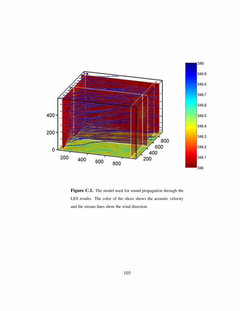
Figure C.1. The model used for sound propagation through the
LES results. The color of the slices shows the acoustic velocity
and the stream lines show the wind direction.
103
9. the slice output filename,
10. and the trace output filename.
This run took 10hr on 100 processors of a Compaq ES45 on the Aeronautical Systems
High Performance Computing machine.
Some results of this simulation are shown in Figure C.2 for slices in the three planes.
For times greater than 0.4 s, we can see a subtle effect of the atmosphere on the acoustic
wave. Here low-amplitude pressure events trail the main diverging wavefronts. This effect
is due to scattering from atmospheric heterogeneities in sound speed, density, and ambient
velocity. It is most prevalent at 1.7s, where there is a small filling in of the field in the right
side of the domain.
104
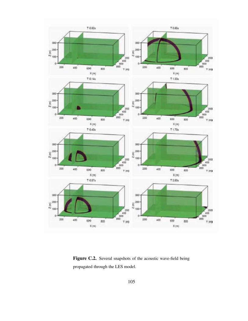
Figure C.2. Several snapshots of the acoustic wave-field being
propagated through the LES model.
105

This page intentionally blank
106
DISTRIBUTION:1 David Marlin
AMSRD-ARL-CI-ES
White Sands Missle Range, NM
88002-5501
1 Keith Wilson
ERDC-CRREL
72 Lyme Rd.
Hanover, NH 03755-1290
1 Rodney W. Whitaker
EES-2 MS J577
Los Alamos, NM 87545
1 Sandra L. Collier
AMSRD-ARL-CI-ES
2800 Powder Mill Road
Adelphi, MD 20783-1197
1 Michael J. White
US Army ERDC/CERL
PO Box 9005
Champaign, IL 61822-1072
1 MS 0750
Neill P. Symons, 06116
1 MS 0750
David F. Aldrige, 06116
1 MS 0750
Lewis C. Bartel, 06116
1 MS 0750
Gregory J. Elbring, 06116
1 MS 1161
Terry K. Stalker, 05432
1 MS 0380
Timothy F. Walsh, 01542
1 MS 1243
Christoper J. Young, 05533
2 MS 9960
Central Technical Files, 8945-1
2 MS 0899
Technical Library, 4536
107