STAJSIC, DAVORIN, M.A. Combinatorial Game Theory (2010)Directed by Dr. Clifford Smyth. pp.40

Given a combinatorial game, can we determine if there exists a strategy for a player

to win the game, and can we pinpoint what this strategy is? The answer to these

questions varies from game to game, and even the most trivial games can become a

burden to solve if we change a few rules, such as playing the game under the misere

play rule. In this paper, we learn some fundamental techniques that are useful to

solving many games. We will analyze the game of Nim and its many variations, and

learn about the Sprague-Grundy function and how to create a single game out of

many. Using the techniques we learned, we analyze and completely solve the Green

Hackenbush game.

COMBINATORIAL GAME THEORY

by

Davorin Stajsic

A Thesis Submitted tothe Faculty of The Graduate School at

The University of North Carolina at Greensboroin Partial Fulfillment

of the Requirements for the DegreeMaster of Arts

Greensboro2010

Approved by

Committee Chair

APPROVAL PAGE

This thesis has been approved by the following committee of the

Faculty of The Graduate School at The University of North Carolina at Greensboro.

Committee Chair

Committee Members

Date of Acceptance by Committee

Date of Final Oral Examination

ii

ACKNOWLEDGMENTS

I would especially like to thank Dr. Clifford Smyth for his patience, guidance

and understanding.

I would also like to thank the committee members, Dr. Paul Duvall and

Dr. Carlos Nicolas, for taking their time to participate in this process, and I want

to thank Dr. Maya Chhetri for her persistence and helping this project come to

fruition. Also, thanks to all my fellow graduate students for their support.

iii

TABLE OF CONTENTS

Page

CHAPTER

I. INTRODUCTION . . . . . . . . . . . . . . . . . . . . . . . . . . . . . . . . . . . . . . . . . . . . 1

II. GRAPH GAMES . . . . . . . . . . . . . . . . . . . . . . . . . . . . . . . . . . . . . . . . . . . . . 4

2.1. P and N positions . . . . . . . . . . . . . . . . . . . . . . . . . . . . . . . . . . . . . . . . . . 5

III. THE GAME OF NIM . . . . . . . . . . . . . . . . . . . . . . . . . . . . . . . . . . . . . . . . . 8

3.1. Overview . . . . . . . . . . . . . . . . . . . . . . . . . . . . . . . . . . . . . . . . . . . . . . . . . . 83.2. Analysis of Nim . . . . . . . . . . . . . . . . . . . . . . . . . . . . . . . . . . . . . . . . . . . . 83.3. Nim-Sum . . . . . . . . . . . . . . . . . . . . . . . . . . . . . . . . . . . . . . . . . . . . . . . . . . 93.4. The Winning Strategies for Nim . . . . . . . . . . . . . . . . . . . . . . . . . . . . . 93.5. Misere Nim . . . . . . . . . . . . . . . . . . . . . . . . . . . . . . . . . . . . . . . . . . . . . . . . 113.6. Moore’s Nim . . . . . . . . . . . . . . . . . . . . . . . . . . . . . . . . . . . . . . . . . . . . . . . 123.7. Wythoff’s Nim . . . . . . . . . . . . . . . . . . . . . . . . . . . . . . . . . . . . . . . . . . . . . 15

IV. THE SPRAGUE-GRUNDY FUNCTION . . . . . . . . . . . . . . . . . . . . . . . 23

4.1. The Sprague-Grundy Function . . . . . . . . . . . . . . . . . . . . . . . . . . . . . . . 234.2. Sums of Games . . . . . . . . . . . . . . . . . . . . . . . . . . . . . . . . . . . . . . . . . . . . . 25

V. GREEN HACKENBUSH . . . . . . . . . . . . . . . . . . . . . . . . . . . . . . . . . . . . . . 29

VI. CONCLUSION . . . . . . . . . . . . . . . . . . . . . . . . . . . . . . . . . . . . . . . . . . . . . . . 39

BIBLIOGRAPHY . . . . . . . . . . . . . . . . . . . . . . . . . . . . . . . . . . . . . . . . . . . . . . . . . . . . . . . 40

iv

1

CHAPTER I

INTRODUCTION

The formal definition of a combinatorial game is quite delicate, as there are

certain conditions that need to be satisfied, and there are a few things that are not

allowed:

Definition 1. (Combinatorial Game) A combinatorial game is a game that

satisfies the following conditions:

• There are two players.

• There is a set of possible positions in the game. This set is usually finite.

• The rules specify all the possible moves between two different positions, for

both players.

• The players alternate moves. A player cannot pass on making a move if it is

his or her turn to move.

• The game ends when a player reaches a position from which no further moves

are possible for the player whose turn it is to move.

• If a game never ends, it is declared a draw. However, most games have the

ending condition, which requires that the game always ends in a finite num-

ber of moves.

A winning position for a player in a combinatorial game is a position that

guarantees the victory for that player. A terminal position is a position from

2

which no other moves are possible, and therefore, the game ends when one of the

player reaches such a position.

Combinatorial games are divided into two categories: impartial and partisan

games. In impartial games, the winning positions and the set of legal moves between

positions is exactly the same for both players. Every other game is classified as a

partisan game. Tic-tac-toe, chess, and checkers are all partisan games, since each

player has a different set of moves available from a typical position. As evidenced by

these examples, some partisan games can result in a tie, where neither player wins

decisively. Under the normal play rule, a player that reaches a terminal position

first is declared the winner of the game. Under misere rule, the first player to reach

a terminal position loses. Unless we explicitly mention it, all games will be played

according to normal play.

Our main goal in the study of a given combinatorial game is to discover

whether either of the players has a specific strategy to reach a terminal position,

therefore forcing the win, under normal play. Under misere play, we are trying to

find a set of moves that forces the opponent to reach the terminal position. If such

a set of moves exists, we call it the winning strategy for that player, and we would

like to discover what this strategy is.

All of the previous definitions are by Ferguson [2].

Now that we are familiar with the concept of combinatorial games, it is time

to introduce a very basic example of such a game, and attempt to a winning strategy,

if one exists. For clarity, when we write Player I or the first player, we are referring

to the player that makes the first move in the given combinatorial game. Player II

or the second player is the player that responds to the first player’s move.

Example 1. Consider a pile of 7 coins, and two players alternating moves, remov-

ing one, two, or three coins from the pile at a time. The player that removes the

3

last coin wins. Find a winning strategy for either of the players, if it exists.

When we analyze combinatorial games, backwards induction is often the best

approach. We find all terminal positions, and then analyze the positions that led

to these terminal positions and then the positions that lead to these and so on. In

our example, there is only one terminal position (a pile of 0 coins). There are three

positions from which we could have made a move to reach this terminal position: a

pile with 1, 2, 3 coins, respectively. Then, from a pile of 4 coins, any move results

in of these three positions. So, if we are starting with 7 coins, the first player can

remove 3 coins to obtain a pile of 4 coins, and then the second player is forced to

move to a position with 1, 2 or 3 coins. The first player then can simply move to

the terminal position and win.

Later in the paper, we will formalize these kinds of arguments into power-

ful tools for the analysis of combinatorial games, the characteristic properties of

positions and the Sprague-Grundy Function. We will then use these tools to ana-

lyze several different types of games. While we are not able to fully solve a game,

in many games we can at least determine which player can win given appropriate

moves.

4

CHAPTER II

GRAPH GAMES

There exists a strong link between combinatorial games and graph theory.

To further analyze this relation, we need to familiarize ourselves with the concept

of directed graphs. Unless specified, the definitions and theorems in this chapter

are by Ferguson [2].

Definition 2. A directed graph G is a pair (X,F ) where X is a non-empty set

of vertices and F is a set of ordered pairs of vertices, called directed edges.

For our purposes, the set X denotes all possible positions in a given game,

and set F contains all possible moves from one position to another one. For a

position x ∈ X, F (x) = {y ∈ X : (y, x) ∈ F} is the set of all possible moves from

position x. F (x) is called the set of followers of x. If a position x has no followers

(in other words, if F (x) is empty), it is called a terminal position.

Let us consider a two player combinatorial game. Player 1 starts at position

x0 ∈ X, and players alternate moves. At a position x, a player whose turn it is to

move moves to a position y so that y ∈ F (x), or a follower of x. The player that

is unable to move loses. We will focus on progressively bounded graphs, in

which every directed path is of finite length, to avoid the situation where our game

could continue indefinitely. Games corresponding to these graphs are also called

progressively bounded, meaning they satisfy the ending condition. If X is finite,

this means that the graph contains no directed cycles.

Recall the simple subtraction game we used in Example 1 in previous section.

Our subtraction set was S = {1, 2, 3}, and our seven chips represent vertices, so

5

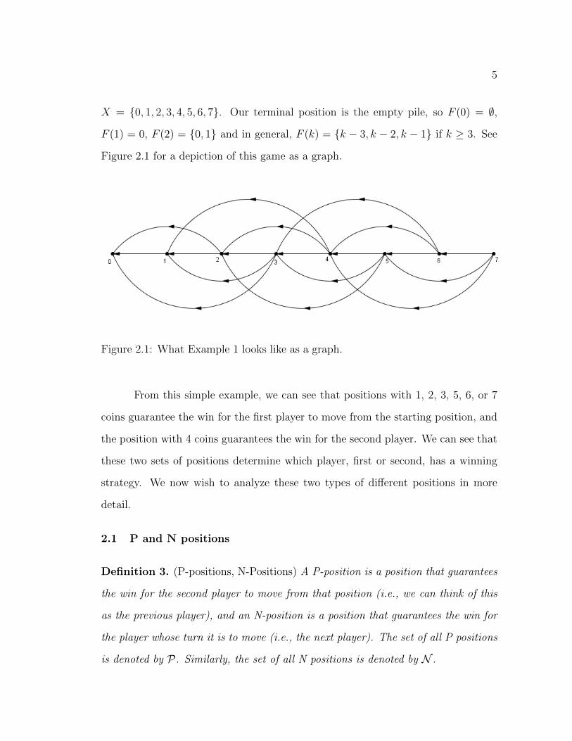
X = {0, 1, 2, 3, 4, 5, 6, 7}. Our terminal position is the empty pile, so F (0) = ∅,

F (1) = 0, F (2) = {0, 1} and in general, F (k) = {k − 3, k − 2, k − 1} if k ≥ 3. See

Figure 2.1 for a depiction of this game as a graph.

Figure 2.1: What Example 1 looks like as a graph. asdfjsa; ldkga;sdkjglsda kjflsad-jfla;ks djflsadfkjlsadf kj;saldkjf sa;ldfkj

From this simple example, we can see that positions with 1, 2, 3, 5, 6, or 7

coins guarantee the win for the first player to move from the starting position, and

the position with 4 coins guarantees the win for the second player. We can see that

these two sets of positions determine which player, first or second, has a winning

strategy. We now wish to analyze these two types of different positions in more

detail.

2.1 P and N positions

Definition 3. (P-positions, N-Positions) A P-position is a position that guarantees

the win for the second player to move from that position (i.e., we can think of this

as the previous player), and an N-position is a position that guarantees the win for

the player whose turn it is to move (i.e., the next player). The set of all P positions

is denoted by P. Similarly, the set of all N positions is denoted by N .

6

For brevity, we may refer to a P-position as P, or N-position as N.

Notice that if the entire set of positions is P ∪ N= X, then one of the

players must have a winning strategy. If the starting position is in N , the first

player to move has a winning strategy. Otherwise, the second player can win given

using appropriate moves. Also, P ∩ N= ∅ because for a position to be P and N

guarantees the win for both players, which cannot happen. Also, if x is a position

in a progressively bounded game, then x ∈ P ∪ N . Perez [6] shows why.

Theorem 1. In a progressively bounded impartial combinatorial game, all positions

x lie in P ∪N .

Proof. Since our game is bounded, it must end in a finite number of moves from any

position. Let b(x) denote the maximum number of moves that the game might last,

from a position x. Using induction on b(x), we show that every position is either P

or N . If b(x) = 0, x is a terminal position, so x ∈ P . Assume the theorem holds

true for all positions x with b(x) ≤ n. Let B denote the set of all those positions.

Consider a position y so that b(y) = n + 1. Then any move from y will take us to

a position in B. We may assume B ⊆ P ∪ N by induction.

If F (y) ⊆ N , then y ∈ P . Otherwise, there exists z ∈ B, a follower of y,

such that z ∈ P . Then, by definition, y ∈ N .

This tells us that every position in a progressively bounded game is either a

P-position or an N-position.

For a given progressively bounded game, it is possible to label each position

as either N or P by working recursively from the terminal positions. We now give

the algorithm for normal play:

1. Label every terminal positions as a P-position.

7

2. Label every position that can reach an already labeled P-position in exactly

one move as an N-position.

3. Find all positions whose every move leads to an already labeled N-position,

and label them as P.

4. If no new positions are found in the previous step, we are done. Otherwise,

repeat the process from step 2.

The algorithm for misere play is the same except we label the terminal po-

sitions as P-positions, and steps 2 and 3 are switched.

In general, when deciding whether a given position is P or N, we need to

check the following three properties:

Characteristic Property. The following three statements define P and N-positions

recursively:

1. All terminal positions are P-positions.

2. From every N-position, there is at least one move to a P-position.

3. From any P-position, every move leads to an N-position

All of these properties were proven in the previous theorem.

We are now ready to introduce a well-studied impartial combinatorial game,

Nim.

8

CHAPTER III

THE GAME OF NIM

3.1 Overview

The Game of Nim is the perfect starting point for studying impartial games, as all

progressively bounded games under normal play are simply Nim in disguise, as we

shall later see. The game of Nim is played as follows:

There are several piles of chips, n in all. Let x1, x2, ..., xn be the number

of chips in piles 1, 2, . . . , n respectively. The game is played between two players.

A move consists of player choosing a pile, and removing at least one chip from

that pile. The player may also choose to remove the whole pile. Whichever player

removes the last chip overall is declared the winner.

3.2 Analysis of Nim

One-pile Nim does not make a very interesting game, since the first player can simply

remove the whole pile and win. Nim with two piles is slightly more complicated.

Assuming the numbers of chips in each pile were unequal to begin with, the winning

strategy for the first player is to maintain the same number of chips in each pile.

Consequently, the second player is always forced to make a move to a position where

piles have a different number of chips. Since the terminal position, (x1, x2) = (0, 0)

contains the same number of chips, the second player cannot reach the terminal

position. Therefore, the first player wins with this strategy. If the number of chips

in each pile is the same in the beginning, the first player is forced to make a move

9

to some position with an uneven number in each pile. The second player can now

use the same strategy as described to win.

3.3 Nim-Sum

The binary numeral system is used heavily in determining the winning strategy for

Nim. For every integer n ≥ 0, there exists a unique sequence ε0, ε1, ε2, . . . so that

εi = 0 or 1, and n =∑∞

i=0 εi2i. We write this as n = (εmεm−1 . . . ε1ε0). Normal

binary addition is performed in the same manner as the regular addition, with

carry. However, for our purposes, we need a slightly different type of sum, defined

by Ferguson [2]:

Definition 4. The nim-sum of (xm...x0)2 and (ym...y0)2 is the binary number

(zm...z0)2, denoted by (xm...x0)2 ⊕ (ym...y0)2 = (zm...z0)2, where for all k, zk =

xk + yk(mod 2).

For our purposes, when performing calculations, we will drop the parentheses

and the subscript 2 in the binary notation. So, for a position (x1, x2, ..., xn) in Nim,

each xi is the number of chips written in binary form xikxi(k−1) . . . xi1xi0 where xij

is 0 or 1.

3.4 The Winning Strategies for Nim

The winning strategy for the game of Nim is best expressed in terms of Nim-sum,

and Ferguson [2] shows the solution:

Theorem 2. (Bouton’s Theorem) A position (x1, x2, ..., xn) in Nim is a P-position

if and only if x1 ⊕ x2 ⊕ . . .⊕ xn = 0.

Proof. Let Z be the set of all positions whose Nim-sum is zero, and let NZ denote its

complementary set, all positions whose Nim-sum is not zero. To prove the theorem,

10

we need to check that Z and NZ satisfy the three characteristic properties of P and

N-positions: all terminal positions are Z, every move from any position in Z leads

to a position in NZ, and there exists at least one move from any position in NZ to

a position in Z.

The only terminal position is t = (0, 0, ..., 0), its Nim-sum is 0 and t ∈ Z.

Now we wish to show that for any given position in Z, every move leads

to a position in NZ. Suppose (x1, x2, ..., xn)∈ Z. Then, x1 ⊕ x2 ⊕ ... ⊕ xn = 0.

Without loss of generality, assume a move is made in the first pile. We obtain a

new pile, y1, with y1 < x1. If we assume the new position, (y1, x2, ..., xn), is in Z,

then y1 ⊕ x2 ⊕ ...⊕ xn = 0. And so,

y1 ⊕ x2 ⊕ ...⊕ xn = 0 = x1 ⊕ x2 ⊕ ...⊕ xn.

Notice that for Nim-sums x ⊕ x = 0, so the cancellation law holds, y ⊕ x = z ⊕ x

implies y = z. By canceling x2, . . . , xn from both sides, we obtain

x1 = y1

which is a contradiction. Therefore, (y1, x2, ..., xn) ∈ NZ.

The only thing that’s left to check is the existence of a move from every

position in NZ to a position in Z. We construct such a move in the following

manner:

For a position (x1, x2, ..., xn) ∈ NZ, let z = x1 ⊕ . . . ⊕ xn 6= 0. There is at

least one i such that zi = 1. Find the largest i so that zi = 1, and pick a pile xj that

has a 1 in the ith entry. By taking away an appropriate number of chips from that

pile, we can change xji from 1 to 0, and also change the digits xj(i−1), xj(i−2), . . . , xj0

to be what ever we want. Thus we can set zi−1 = zi−2 = . . . = z0 = 0 as well. We

need to remove exactly xj − (z⊕xj) chips from the jth pile. This leaves the jth pile

with z ⊕ xj chips, and the Nim-sum of the piles becomes 0. This is a legal move

11

because b = z ⊕ xj has all bits bl = 0 for l ≥ i. Thus b ≤ 2i − 1 < 2i ≤ xj, i.e.

b < xj.

Since Z and NZ possess the same characteristic properties as P and N-

positions, Z = P and NZ = N .

3.5 Misere Nim

Under misere play rule, the terminal position (0, 0, ..., 0) is the only N-terminal

position, and therefore all positions (1, 0, . . . , 0), (0, 1, 0, . . . , 0), . . . , (0, 0, . . . , 0, 1)

are P-positions. Let us assume that all of our piles are of size 1. We can observe

that positions that have an odd number of piles with 1 chip are in P , and the ones

with an even number are in N . Bouton determined a winning strategy for Nim

under misere play based on reducing the game to an odd number of piles of size 1.

Ferguson [2] explains:

Assuming the starting position has a non-zero Nim-sum, the first player can

win. The game is split into two states. The first state of the game is when there

are two or more piles with more than one chip. The first player can win by playing

the game as if it were regular Nim, i.e., P-positions are those whose Nim-sum is 0

as long as there are two or more piles with more than one chip.

When the opponent makes a move and reduces the game to exactly one pile

with more than one chip , we are in the second state of the game. This is guaranteed

to happen because optimal play in ordinary Nim never requires the first player to

leave a single pile of size greater than 1, since the Nim-sum resulting from playing

the winning strategy is always 0. Also, the opponent cannot make a move from

two or more piles of size greater than 1 to none. The P-position for the first player

is obtained by making the move in the large pile, reducing it to zero or one chip,

12

whichever leaves odd number of piles of size 1 in play. Then the second player is

forced to remove the last chip.

In general, the Misere version of combinatorial games is much more compli-

cated to analyze and solve, even if the game under normal play is trivial.

3.6 Moore’s Nim

In 1910, E. H. Moore [5] invented Nimk, a generalization of Nim. As in Nim, there

are n chips divided into piles, however, we may now remove any number of chips

from each of a set of up to k piles. Therefore, Nim1 is the ordinary game of Nim.

To solve Nimk, we define a sum analogous to Nim-Sum:

Definition 5. (Nimk-Sum) For a position (x1, x2, ..., xn) in Moore’s Nim, the Nimk-

sum, denoted by ⊕k(x1, x2, ..., xn), is a number expressed as ym . . . y0 where yi ≡

x1i + x2i + . . .+ xni mod (k + 1) and 0 ≤ yi ≤ k for all i.

The definition and the following theorem are due to Moore [5], as shown by

Peres [6].

Theorem 3. (Moore’s Theorem) A position (x1, x2, ..., xn) is a P-position if and

only if its Nimk-sum is 0. Therefore, a position is an N-position if and only if its

Nimk-sum is not 0.

To better understand the theorem and the following proof, it helps to view

this addition in terms of rows and columns. Each pile written in binary corresponds

to one row, and for each j,m ≥ j ≥ 0, column j corresponds to a set consisting of

x1j, x2j, . . . , xnj:

x1 = x1mx1(m−1) . . . x10

x2 = x2mx2(m−1) . . . x20

13

xn = xnmxn(m−1) . . . xn0

Our theorem tells us that a position is a P-position if the sum of entries in

each column of the binary representation of addition is divisible by k + 1.

Proof. To prove the theorem, it is sufficient to show that our candidates for P-

positions and N-positions satisfy the three characteristic properties:

1. The only terminal position is (0, 0, ..., 0), and it is a P-position since the sum

of piles is zero.

2. It is possible to construct a move from a position whose Nimk sum is not zero

to a position whose Nimk sum is zero in the following manner:

Consider the left-most column whose sum s is not divisible by k + 1. Let

s ≡ r mod (k + 1), where r ∈ {1, 2, ..., k}. Select r rows whose entry in

that column is 1. Changing these entries to 0 constitutes a legal move in

a game of Nim, and for that column, the new sum is s∗ ≡ 0 mod (k + 1).

For the remainder of this process, we are able to adjust any xij entry to the

right of this column in the selected rows as we desire, since this still qualifies

as a legal move. We proceed to the new left-most column whose sum s1 6≡

0 mod (k + 1), ignoring the rows already selected. Let q ≡ s1+r mod (k + 1),

q ∈ {0, 1, ..., k}.

This leads to two cases. If q ≤ r, set the xij in q rows of the already selected

rows to 0, and those in the other r − q rows to 1. Then the new sum in this

column is divisible by k + 1. If r < q, then we can select an additional q − r

of the previously non-selected rows that have a 1 in this column, and then

changing the entries of all selected rows to 0 in this column gives us a sum

that is divisible by k + 1.

We proceed with the step above if necessary until all columns have a Nimk-

14

sum of 0 or until we select k rows. When we select k rows, the sum in any

of the remaining columns will be between 0 and k, disregarding the selected

rows. If the sum in a column is 0 mod (k + 1), set every entry in the k selected

rows to 0. Otherwise, we have enough free rows to make each sum a multiple

of k + 1.

3. Assume the game is currently in a position x where the Nimk sum of all piles

is 0. Given an arbitrary move, consider the left-most column where a change

has occurred in the binary expansion. In x, the sum of entries in this column

was divisible by k + 1. In this column, in order for a move to be legal, some

1’s had to be changed to zeros, otherwise we would be increasing the number

of chips. Since we are removing chips from up to k piles, and 1’s are changed

into zeros in this given column, the sum will decrease by at least 1, and at

most k, and the new sum cannot be divisible by k+ 1. Therefore, every move

from a position whose Nimk sum is zero leads to a position whose Nimk is not

zero.

It is interesting to note that for misere Nimk, the winning strategy is a simple

extension of the strategy for misere Nim. Recall that in misere Nim the strategy

involved playing the winning strategy under the regular rules as long as there are

at least 2 piles whose size is greater than 1.

Theorem 4. The first player has a winning strategy in misere Nimk precisely when

the Nimk-sum of the starting position is not zero. When there are k + 1 or more

piles with more than 1 chip, P-positions are those whose Nimk-sum is 0. When

there are k or less piles with more than 1 chip, we reach a P-position by reducing

all of those piles to either 0 or 1 in order to obtain a Nimk-sum of 1.

15

Proof. The winning strategy for the first player is as follows:

As long as there are at least k+1 piles whose size is greater than 1, play as if

the game were regular Nimk. That is, the P-positions are those whose Nimk-sum is

0, if there are more than k + 1 piles with more than one chip. When the opponent

makes a move so that there are n ≤ k piles of size greater than 1, and r ≥ 0 piles of

size 1, the first player reduces all n piles to 0 or 1, whichever yields a Nimk sum of

1 when summed with those r piles. In other words, when the second player makes

a move so that there are k+ 1 or less piles with more than one chip, P-positions are

those whose Nimk-sum is 1 after reducing all those piles to 0 or 1 chip.

This is guaranteed to happen because the first player cannot make a move

to a position with k or less piles each of size greater than 1, since such positions

don’t have a Nimk sum of 0. Therefore, the second player is forced to make such a

move and furthermore is forced to leave a number of piles n, with 1 ≤ n ≤ k. When

the first player reduces all those piles to 0 or 1 so that the Nimk-sum is 1, the game

essentially becomes a misere take away game with k chips, and the second player is

moving from a P-position. Therefore, the first player has a winning strategy.

3.7 Wythoff’s Nim

Wythoff [8] came up with a Nim-like game, Wythoff’s Nim which is played on only

two piles of sizes m and n respectively. Peres [6] investigates it. Legal moves are

the same as those of Nim, with an additional option to remove the same number of

chips from both piles. Thus, our legal moves consist of reducing m to some value

between 0 and m− 1 without changing n, reducing n to some value between 0 and

n − 1 without changing m, or reducing both n and m by the same amount. Note

that this immediately implies that (k, k) /∈ P , for k > 0 ( (0, 0) is the terminal

position).

16

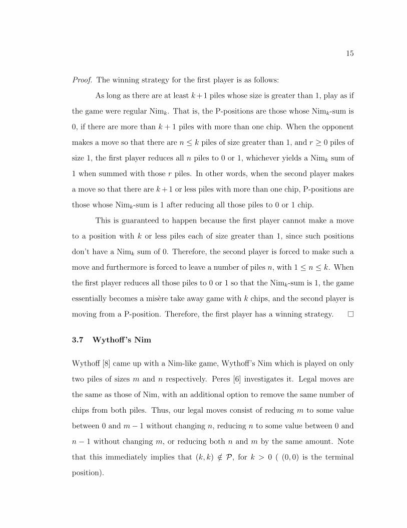
Before we analyze this game, consider another game played on a chessboard

of arbitrary size n by m. A queen piece is positioned in the upper right corner of the

board. Two players alternate moving the queen down, left, or diagonally towards

the bottom left corner. The player who reaches the bottom left corner wins.

Figure 3.1: Corner the Queen, same as Wythoff’s Nim. For more details, seePeres [6]. asdfas gsadgsag dsdagfsadgsafgsd algjsa;lghkjsaldfjkfjs da;lfkjsa;ldfkjsa;ldfkjsda;l

Let us denote the position of the queen by (x, y), where 0 ≤ x ≤ n and

0 ≤ y ≤ m. Considering legal moves of the queen, we see that this game is simply

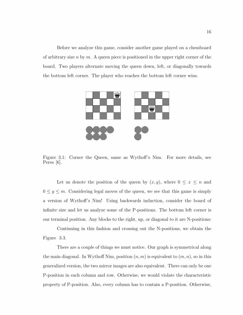
a version of Wythoff’s Nim! Using backwards induction, consider the board of

infinite size and let us analyze some of the P-positions. The bottom left corner is

our terminal position. Any blocks to the right, up, or diagonal to it are N-positions:

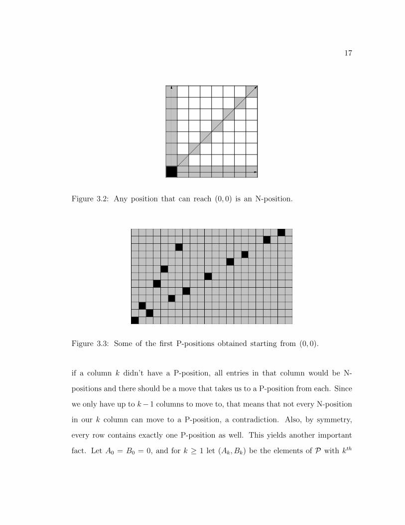
Continuing in this fashion and crossing out the N-positions, we obtain the

Figure 3.3.

There are a couple of things we must notice. Our graph is symmetrical along

the main diagonal. In Wythoff Nim, position (n,m) is equivalent to (m,n), so in this

generalized version, the two mirror images are also equivalent. There can only be one

P-position in each column and row. Otherwise, we would violate the characteristic

property of P-position. Also, every column has to contain a P-position. Otherwise,

17

Figure 3.2: Any position that can reach (0, 0) is an N-position. asdfas gsadgsagdsdagfsadgsafgsd algjsa;lghkjsaldfjkfjs da;lfkjsa;ldfkjsa; ldfkjsda;l

Figure 3.3: Some of the first P-positions obtained starting from (0, 0). sagsgjaslkdj;kfjls da;kfj;l sdakj;sd ajfa;ldkj asd;lfkj

if a column k didn’t have a P-position, all entries in that column would be N-

positions and there should be a move that takes us to a P-position from each. Since

we only have up to k− 1 columns to move to, that means that not every N-position

in our k column can move to a P-position, a contradiction. Also, by symmetry,

every row contains exactly one P-position as well. This yields another important

fact. Let A0 = B0 = 0, and for k ≥ 1 let (Ak, Bk) be the elements of P with kth

18

smallest x-coordinate among those above the line y = x. We have

P = {(0, 0)} ∪ {(Ak,Bk) : k ≥ 1} ∪ {(Bk,Ak) : k ≥ 1}

and {Ak : k ≥ 1} and {Bk : k ≥ 1} form a partition of N∗ = {1, 2, . . .}.

k 0 1 2 3 4 5 6 7 8 9 . . .Ak 0 1 3 4 6 8 9 11 12 14 . . .Bk 0 2 5 7 10 13 15 18 20 23 . . .

Notice that both Ak and Bk are increasing sequences, and Bk > Ak for k ≥ 1.

It turns out that these two sequences can be defined recursively. First, we

need to know what the minimal excludant of a set is, as defined by Conway [1]:

Definition 6. For a set S of non-negative integers, the textminimal excludant or

mex of S is the smallest non-negative integer n so that n 6∈ S.

For example, if S = {0, 2, 4, 6}, then mex(S) = 1, since 1 is the smallest

integer not in this set.

We define two sequences: for k ≥ 0, let

ak = mex{a0, . . . , ak−1, b0, . . . , bk−1, }

bk = ak + k.

Note that for k = 0, a0 = mex{∅} = 0 and b0 = ak + 0 = 0.

We now show that Ak = ak and Bk = bk for all k ≥ 0. It’s easy to check the

following two theorems due to Wythoff [8]:

Theorem 5. {ai}∞i=1 and {bi}∞i=1 form a partition of N∗.

Proof. We show by induction on j that {ai}ji=1 and {bi}ji=1 are two disjoint strictly

increasing subsets of N∗. This is true when j = 0, since both sets are empty.

19

Suppose {ai}j−1i=1 and {bi}j−1i=1 are disjoint and strictly increasing. From the way the

ai are defined, aj, aj−1 /∈ {a0, a1, . . . , aj−2, b0, b1, . . . , bj−2}, but aj−1 is the mex of

that set so aj−1 < aj. Since aj /∈ {b0, . . . , bj−1}, {ai}ji=1 and {bi}j−1i=1 are disjoint.

Also, for each i < j,

bj = aj + j > ai + j > ai + i = bi > ai

and {bi}ji=1 is also disjoint from {ai}ji=1, and is increasing.

We now show that {ai}ji=1∪{bi}ji=1 includes every integer in {1, . . . , j}. This

is true for j = 0. If it is true for j, then j + 1 is either in {ai}ji=1 ∪ {bi}ji=1, or it is

excluded, in which case aj+1 = j + 1, by the definition of aj+1.

Therefore, the theorem holds.

Theorem 6. P for Wythoff’s Nim is precisely W = {(ak, bk) : k = 0, 1, 2, . . .} ∪

{(bk, ak) : k = 0, 1, 2, . . .}.

Proof. We need to check the three characteristic properties of P-positions.

The only terminal position is (0, 0), which is in W .

Consider (m,n) = (ak, bk) ∈ W . By definition, bk − ak = k, so piles m and

n differ in k chips. If we reduce both piles by some amount, the difference between

them is still k, and the only position in W with that difference is (ak, bk), from the

way the sequences are defined. If we reduce m, n only occurs with m in W , and

similarly, if we reduce n, m occurs only with n in W . So any move from W leads

to a position not in W .

Let (m,n) /∈ W with m ≤ n, and let k = n −m. If m > ak and n > bk, we

can reduce both piles to (ak, bk) since ak and bk differ in k chips. Otherwise, either

m = aj or m = bj for some j < k. If m = aj, we can remove k − j chips from n to

get (aj, bj) ∈ W . If m = bj for some j, then n ≥ m = bj > aj, so we can reduce n

to aj and go to position (bj, aj) ∈ W .

20

Therefore, W =P .

Now we wish to show that there exists a quick way to check if a given position

is in P .

Theorem 7. For k ≥ 0, ak = bk(1+√5)

2c and bk = bk(3+

√5)

2c, where bxc denotes the

greatest integer n so that n ≤ x.

Proof. Let αk(θ) = bkθc and βk(θ) = b k

1−θc, for some fixed irrational θ ∈ (0, 1).

Our goal is to show that {αk(θ)}∞k=1 and {βk(θ)}∞k=1 form a partition of N∗,

and then find θ so that αk(θ) = ak and βk(θ) = bk.

For any k, αk ≤ αk+1, and similarly, βk ≤ βk+1. Now, αk(θ) = N if and only

if

N ≤ k

θ< N + 1,

θN ≤ k < θN + θ.

Also, βl(θ) = N if and only if

N ≤ l

1− θ< N + 1,

θN + θ − 1 < −l +N ≤ θN.

There is exactly one integer m in the interval (θN + θ − 1, θN + θ). Since

θ is irrational, m 6= Nθ. Thus either m is in (θN, θN + θ) and αk = N , or m is in

(θN + θ − 1, θN), and βl = N . Therefore, {αk(θ)}∞k=1 and {βk(θ)}∞k=1 are disjoint

and form a partition of N∗.

Now we want to find a θ so that

αk(θ) = ak, βk(θ) = bk.

Since bk = ak + k, we are looking for a solution to

21

⌊k

θ

⌋+ k =

⌊k

1− θ

⌋

Then,

1

k

⌊k

θ

⌋+ 1 =

1

k

⌊k

1− θ

⌋

limk→+∞

1

k

⌊k

θ

⌋+ 1 = lim

k→+∞

1

k

⌊k

1− θ

⌋1

θ+ 1 =

1

1− θ

Therefore, θ2 + θ−1 = 0, and θ =√5−12

= 21+√5∈ (0, 1), while the other root

is negative. This number θ is also known as Φ, or the inverse of the golden ratio.

Let us consider αk(θ) and βk(θ) for θ = 21+√5. Since Φ satisfies

1

Φ+ 1 =

1

1− Φ

then

k

Φ+ k =

k

1− Φ

.

Since k is an integer, taking floor of both sides we obtain

⌊k

1− Φ

⌋=

⌊k

Φ

⌋+ k

so βk = αk + k.

The only property left to check is

αk = mex{α0, α1, . . . , αk−1, β0, β1, . . . , βk−1}.

22

We know that αk can’t be any of the values in the set of excludants. It

remains to show that it is in fact the mex of all these values. By way of contradiction,

suppose αk 6= m = mex{α0, α1, . . . , αk−1, β0, β1, . . . , βk−1}. Then m < αk ≤ αl ≤ βl

for all k ≤ l. For i ∈ {0, 1, . . . , k − 1}, m 6= αi, βi, and since αk, βk span N∗, m is

missed. Therefore, αk = mex{α0, α1, . . . , αk−1, β0, β1, . . . , βk−1}.

So, ak = bk(1+√5)

2c and bk = bk(3+

√5)

2c.

Wythoff [8] himself said that he came up with this discovery “out of a hat”.

23

CHAPTER IV

THE SPRAGUE-GRUNDY FUNCTION

4.1 The Sprague-Grundy Function

Now that we know a combinatorial game can be represented by a directed graph,

we need tools to analyze the game from this new perspective.

Definition 7. The Sprague-Grundy function of a progressively bounded graph

(X,F ) is a function g defined on X, so that for x ∈ X,

g(x) = mex{g(y) | y ∈ F(x)}.

Perez [6] defines the Sprague-Grundy function (SG for short) recursively, and

as such, it is appropriate to start analyzing SG function of a graph starting with

terminal positions. Since a terminal position t has no followers, F (t) = ∅, and their

SG value is therefore g(t) = 0. All positions that only lead to a terminal position

therefore have SG value of 1.

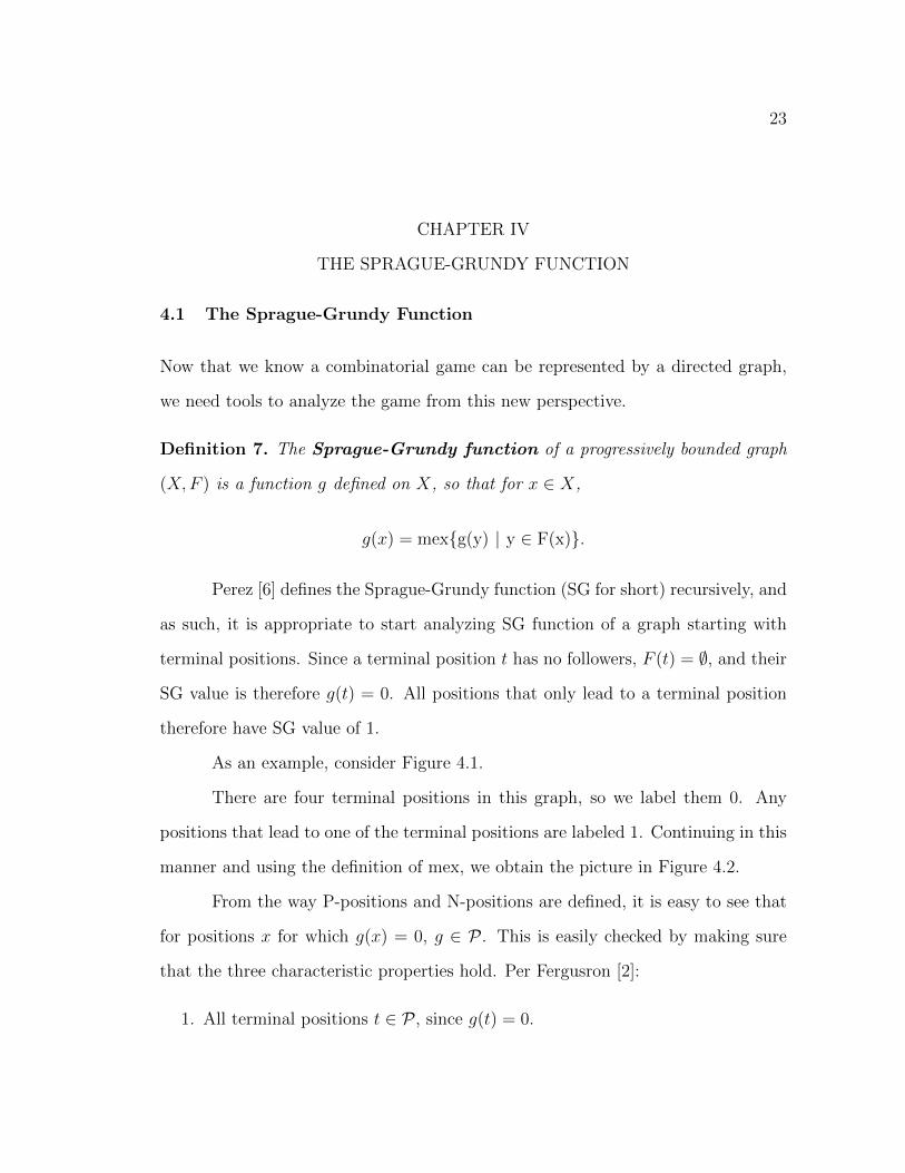
As an example, consider Figure 4.1.

There are four terminal positions in this graph, so we label them 0. Any

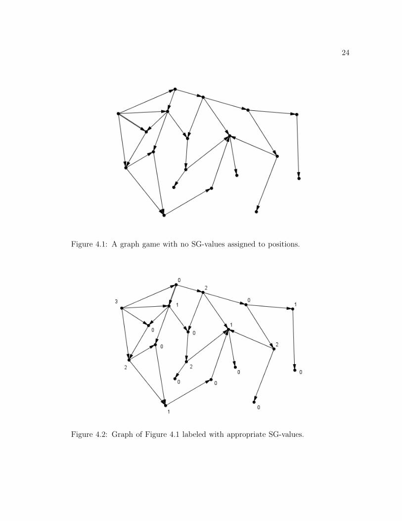
positions that lead to one of the terminal positions are labeled 1. Continuing in this

manner and using the definition of mex, we obtain the picture in Figure 4.2.

From the way P-positions and N-positions are defined, it is easy to see that

for positions x for which g(x) = 0, g ∈ P . This is easily checked by making sure

that the three characteristic properties hold. Per Fergusron [2]:

1. All terminal positions t ∈ P , since g(t) = 0.

24

Figure 4.1: A graph game with no SG-values assigned to positions. lasdfjalsgdjls-dakjga;lksdjflsdakfjlsda;kjflsda;fkjasld;fkjasd;lkfjsa;f

Figure 4.2: Graph of Figure 4.1 labeled with appropriate SG-values. asdfa nnsdf-sagsdagf ufgkjgkj jfgjgfkj lkgh asdgsnn adfgasdsdafa

25

2. For a position x, let g(x) = 0. Assume there exists a follower y ∈ F (x) so

that g(y) = 0. But this cannot happen, since in that case x itself cannot have

SG value of 0, from our definition of mex. So every follower of x has SG value

different from 0.

3. For a position x so that g(x) 6= 0, there must exist at least one follower y so

that g(y) = 0. If this was not true, then the SG-value of x itself would have

to be 0, from the way mex is defined.

4.2 Sums of Games

For any collection of combinatorial games, we can create a new game that contains

all of them. This game is played just like any other combinatorial game. Players

alternate moves, and a move consists of a player picking a game and performing a

legal move, as defined for that game. The first player unable to make a move loses.

Definition 8. (The Sum of Graph Games) Let G1 = (X1, F1) and G2 = (X2, F2)

be two progressively bounded graphs. G = (X,F ) is the sum of G1 and G2, denoted

by G = G1 +G2 if X = X1 ×X2, and for each (x1, x2) ∈ X, the set of followers is:

F (x1, x2) = ( F (x1)× {x2} ) ∪ ( {x1} × F (x2) ).

Naturally, we can sum more than two games in the same manner.

For example, a Nim game with 2 or more piles is simply a sum of several

single-pile Nim games. While a single Nim pile is a very basic game, a three pile

Nim is not quite so simple. This is true in general sums. Also, since each Gi

is progressively bounded, the sum itself is progressively bounded, and the total

number of moves is the sum of number of moves in each Gi.

Now that we are familiar with the sum of games, we can define what it means

for two games to be equivalent. The definition is due to Perez [6].

26

Definition 9. Consider any two arbitrary combinatorial games G1 and G2, with

positions x1 and x2, respectively. For some arbitrary combinatorial game H with

position h, consider two sum games G1 +H and G2 +H. If the outcome of (x1, h)

in G1 + H is the same as the outcome in (x2, h) in G2 + H, then G1 and G2 are

equivalent.

The following theorem (due to Perez [6]) shows that any progressively bounded

combinatorial game is equivalent to some Nim pile. Note that the SG-value of

any single Nim pile of size k is just k, since the followers of a k-chip pile are

k − 1, k − 2, . . . , 1, and 0.

Theorem 8. Let G be a progressively bounded impartial combinatorial game under

normal rules, with starting position x. Then G is equivalent to a Nim pile of size

g(x).

Proof. Let G be a progressively bounded graph for a combinatorial game whose

SG-value is n. Let N be a Nim pile of size n, and let A be any arbitrary graph for a

game. Consider the two games, G+A and N +A. Assume player Q has a winning

strategy for N +A. This can be either the first or the second player. If we can show

this player also has a winning strategy for G+A, this shows that the two games G

and N are equivalent.

For every move in N + A, we can perform a corresponding move in G + A.

If a move is made in the A portion of the game, the other player responds with

the same move in G + A. If a player makes a move in the N part of N + A, thus

taking its SG-value to some m < n then the next player can respond by making a

move in G and taking its SG-value to m. Notice that m has to be smaller than n,

since removing something from a Nim pile lowers its SG-value. Also, from the way

the Sprague-Grundy function is defined, there must exist a move in G to make it’s

27

SG-value m. Notice that not every move in G + A has a corresponding move in

N +A. It is possible to make a move in G so that the new SG-value is greater than

x, since a follower of a position does not have to have a smaller SG-value. If such

a move is made in G, it is impossible to mimic that move in N .

Player Q can use the exact same strategy as used for N +A, with one minor

addition to compensate for the moves in G+A that don’t have corresponding move

in N +A. If the other player makes a move in G that takes its SG-value to m > n,

then player Q can perform a move in G to bring the SG-value back to n. This

is possible since n has to be a follower of m, from the way SG-values are defined.

These two moves cancel each other out, and since G is progressively bounded, only

a limited number of such moves can be made, and player Q can always respond to

them to bring the game to the original state in terms of SG-values.

Therefore, if the first or second player has a winning strategy for G+A, that

player also has a winning strategy for G+N , and G and N are equivalent.

For a sum of games where we know the SG-value of each individual game,

it is only natural to ask ourselves if there’s a way to calculate the SG-value of this

sum. The following is due to Sprague [7] and Grundy [3].

Theorem 9. (The Sprague-Grundy Theorem) If gi is the Sprague-Grundy func-

tion of Gi, i = 1, ..., n, then G = G1 + ... + Gn has Sprague-Grundy function

g(x1, ..., xn) = g1(x1)⊕ g1(x2)⊕ ...⊕ gn(xn).

Proof. Let x = (x1, ..., xn) be an arbitrary point of X. Let b denote the Nim sum

of all Sprague-Grundy numbers of each xi, b = g1(x1) ⊕ ... ⊕ gn(xn). We need to

show that no follower of x has SG-value of b, and that for every non-negative integer

a < b, there exists a follower of x that has SG-value of a.

To show that no follower of x has the same SG-value, let us assume that

28

the opposite holds. So x has a follower of the same SG-value. Without loss of

generality, supposed a move is made in the first game, so (x′1, x2, ..., xn) is a follower

of (x1, x2, ..., xn) satisfying g1(x′1)⊕g2(x2)⊕...⊕gn(xn) = g1(x1)⊕g2(x2)⊕...⊕gn(xn).

Since the cancellation law holds in modular arithmetic, g1(x′1) = g1(x1). Since no

position can have a follower of the same SG-value, this is a contradiction.

Now we need to show that for a < b, x has a follower whose g-value is b.

Let d = a ⊕ b, and let k denote the number of digits in the binary expansion of d.

Then, d has a 1 in the kth position from the right since the left most digit is always

1 in a binary expansion of a number. From our assumption, a < b so b has a 1

and a has a 0 in the kth position, otherwise their Nim sum would not be d. Since

b = g1(x1) ⊕ ... ⊕ gn(xn), there is at least one xi whose binary expansion of gi(xi)

contains a 1 in kth position. Without loss of generality, assume i = 1. Consider

d⊕ g1(x1), which has a 0 in the kth position. Then d⊕ g1(x1) < g1(x1). Therefore,

there exists a move from x1 to some x′1 with g1(x′1) = d ⊕ g1(x1). Also, the move

from (x1, ..., xn) to (x′1, ..., xn) is a legal move in G, with

g1(x′1)⊕ g2(x2)⊕ ...⊕ gn(xn) = d⊕ g1(x1)⊕ g2(x2)⊕ ...⊕ gn(xn) = d⊕ b

Observe that d⊕ b = a⊕ b⊕ b = a.

Therefore, the Sprague-Grundy theorem holds.

29

CHAPTER V

GREEN HACKENBUSH

A rooted graph is an undirected graph where every vertex is connected to one

of a set of specific nodes called the root or the ground. In a game of Hackenbush,

players take turns deleting an edge from the rooted graph, and then deleting the

components that are no longer connected to any vertex connected to the ground.

When a player deletes an edge, we will say that he chopped the edge. There are

several versions of this game. The impartial version is Green Hackenbush in which

both players may chop any edge they wish. The edges are considered to be all colored

green in Green Hackenbush. The partisan version is called Blue-Red Hackenbush,

consisting of red and blue colored edges. In this version, one player may only chop

blue edges, and the other may only chop red ones. The general game of Hackenbush

combines these two versions: one player removes blue edges, other removes red

edges, and either player can remove green edges. More information about those can

be found in On Numbers and Games by Conway [1].

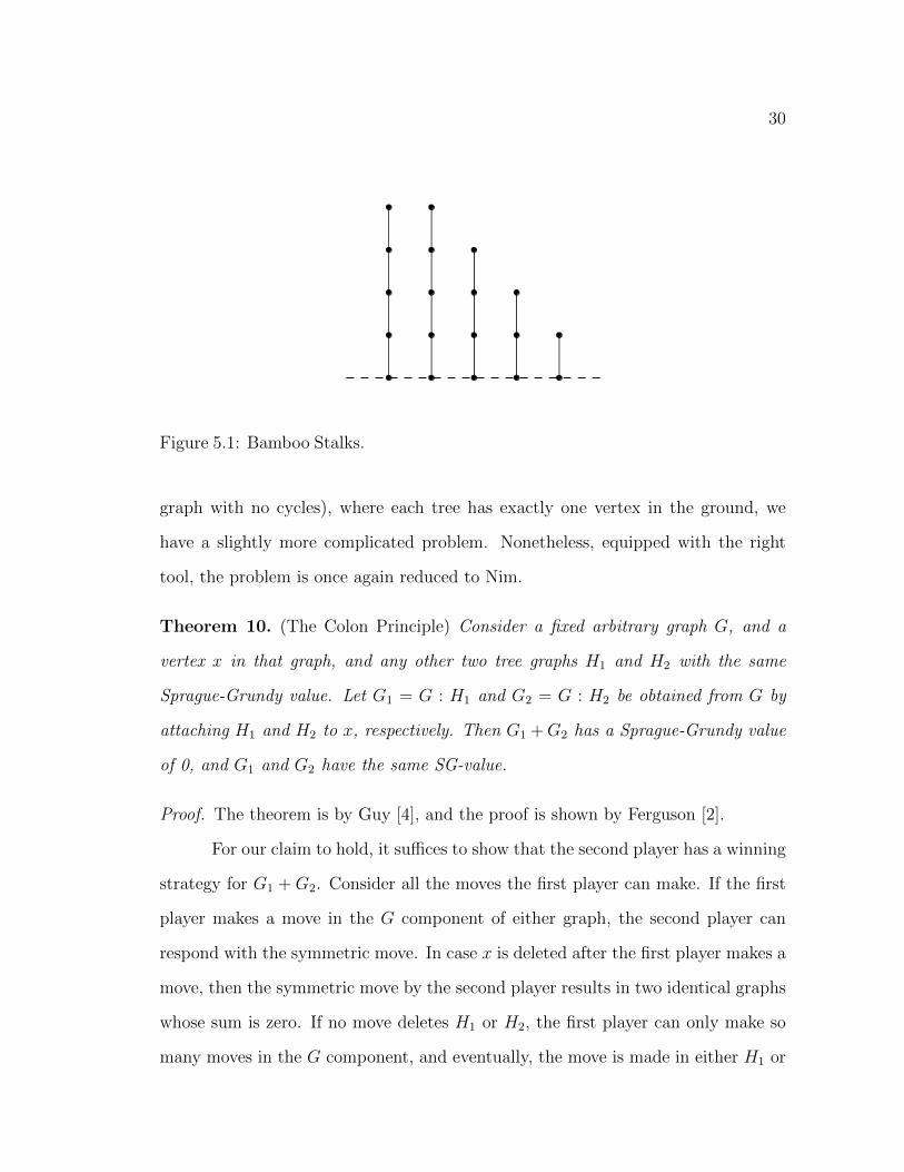
Lets consider the simplest example of Green Hackenbush, bamboo stalks:

A bamboo stalk is a finite length path, with no other edges attached to any

vertices, with one end-vertex being attached to the ground or some other vertex in

the graph, and the other end-vertex is a pendant vertex. Our game consists of a

finite set of bamboo stalks. Thus a move consist of selecting an edge, and removing

it and all the edges above. The player that removes the last segment of the group of

bamboo stalks wins. This is just Nim, where chips are represented by segments of

the bamboo stalk. Therefore, we already know the winning strategy for this game!

If we replace bamboo stalks with a collection of trees (a tree is a connected

30

Figure 5.1: Bamboo Stalks. lsadjfa;l sdjflasdjg sa;ldkj;ljfl; sadkjf;lsa dkjf;lsakd jf;asdlkfjsa; ldfj;

graph with no cycles), where each tree has exactly one vertex in the ground, we

have a slightly more complicated problem. Nonetheless, equipped with the right

tool, the problem is once again reduced to Nim.

Theorem 10. (The Colon Principle) Consider a fixed arbitrary graph G, and a

vertex x in that graph, and any other two tree graphs H1 and H2 with the same

Sprague-Grundy value. Let G1 = G : H1 and G2 = G : H2 be obtained from G by

attaching H1 and H2 to x, respectively. Then G1 +G2 has a Sprague-Grundy value

of 0, and G1 and G2 have the same SG-value.

Proof. The theorem is by Guy [4], and the proof is shown by Ferguson [2].

For our claim to hold, it suffices to show that the second player has a winning

strategy for G1 +G2. Consider all the moves the first player can make. If the first

player makes a move in the G component of either graph, the second player can

respond with the symmetric move. In case x is deleted after the first player makes a

move, then the symmetric move by the second player results in two identical graphs

whose sum is zero. If no move deletes H1 or H2, the first player can only make so

many moves in the G component, and eventually, the move is made in either H1 or

31

H2 since our graph is progressively bounded. Without loss of generality, assume the

first player makes a move in H1, obtaining some H′1 with the SG-value of k. If k is

smaller than the SG-value of H1, the second player moves in H2 to a follower whose

SG-value is k. If k is larger than the SG-value of H1, the second player moves in

H1 to a follower whose SG-value is equal to the original SG-value of H1 (this move

can be considered a “pause”, and only finitely many such “pauses” can occur).

Therefore, for every move the first player makes, the second player has a

corresponding move, and since the game is progressively bounded, the second player

will reach the terminal position.

The following is a direct result of the Colon Principle. A branch is a collec-

tion of stalks that share a common vertex.

Corollary 1. When multiple stalks of a tree come together at a vertex, they can be

replaced with a single stalk of length equal to the Nim-sum of stalks making up the

branch.

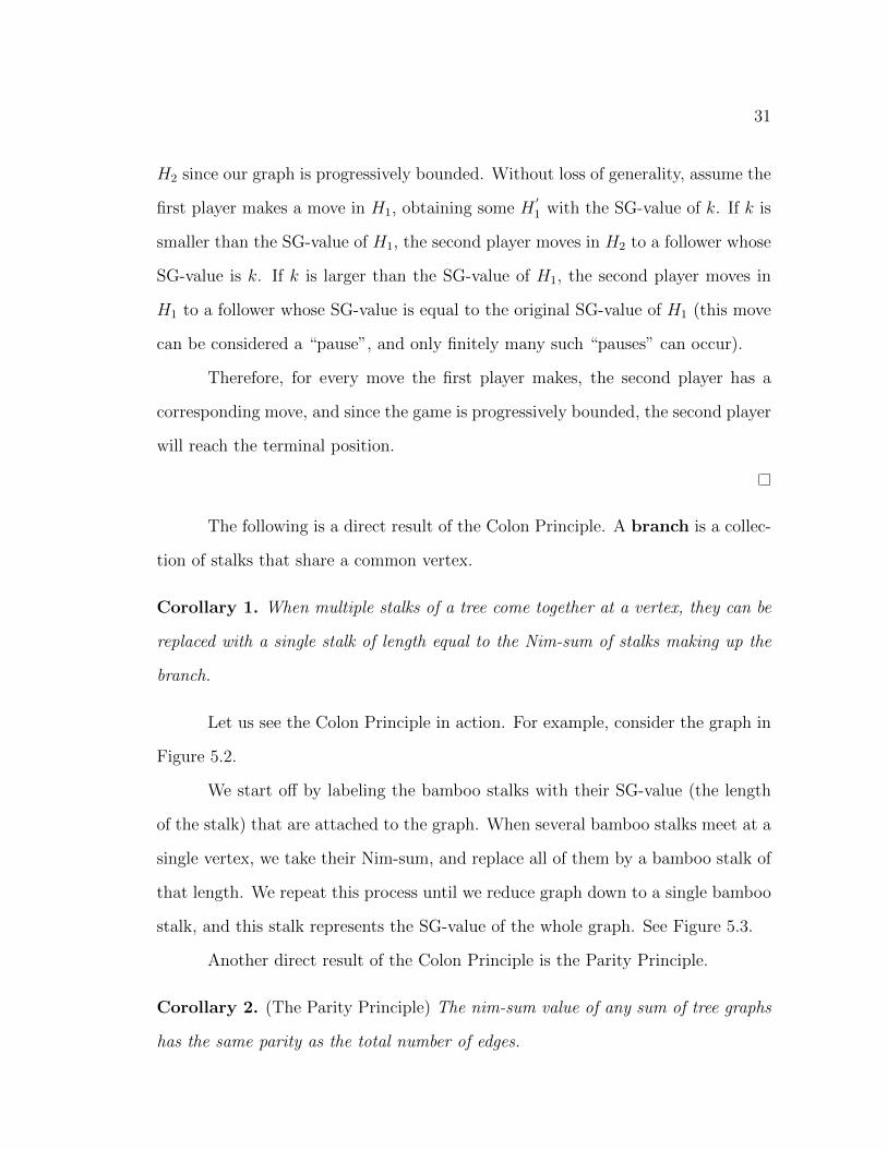
Let us see the Colon Principle in action. For example, consider the graph in

Figure 5.2.

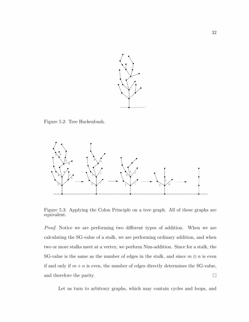
We start off by labeling the bamboo stalks with their SG-value (the length

of the stalk) that are attached to the graph. When several bamboo stalks meet at a

single vertex, we take their Nim-sum, and replace all of them by a bamboo stalk of

that length. We repeat this process until we reduce graph down to a single bamboo

stalk, and this stalk represents the SG-value of the whole graph. See Figure 5.3.

Another direct result of the Colon Principle is the Parity Principle.

Corollary 2. (The Parity Principle) The nim-sum value of any sum of tree graphs

has the same parity as the total number of edges.

32

Figure 5.2: Tree Hackenbush. asdfdfgsadl fkjasd;lgkj sdaljflsad jf;lafdjals dfja;lsdfkjas;lfdjs a;ldkfj sa;ld fjsa;ldfj

Figure 5.3: Applying the Colon Principle on a tree graph. All of these graphs areequivalent. sdfasdlgsajlfjasdljsdal;fjsad;lfjasdlf

Proof. Notice we are performing two different types of addition. When we are

calculating the SG-value of a stalk, we are performing ordinary addition, and when

two or more stalks meet at a vertex, we perform Nim-addition. Since for a stalk, the

SG-value is the same as the number of edges in the stalk, and since m⊕ n is even

if and only if m+ n is even, the number of edges directly determines the SG-value,

and therefore the parity.

Let us turn to arbitrary graphs, which may contain cycles and loops, and

33

with multiple paths attached to the ground. Since any graph is equivalent to a Nim

pile, our goal is to somehow find a tree that is equivalent to a given graph. This

tree is then equivalent to a Nim pile, using the Colon principle.

In graph theory, by identifying vertices u and v in a graph we obtain a

new graph where the two vertices are replaced by a single vertex w, with each

edge between u and v replaced by a loop at w, and where edges that were incident

on u or v are redirected to w. All other edges remain unchanged. We can apply

this to a cycle in a graph: we simply contract all the edges by identifying any two

or more vertices in the cycle by repeated application of identifying vertices. This

process is called fusing by Conway and Guy [4]. For Green Hackenbush we can also

replace any loops with a single edge, where one end is unattached. With repeated

application of fusing and the Colon Principle, we can shrink any graph down to a

single stalk. We now show that the stalk obtained by this procedure has the same

SG-value as the original graph. The groundwork for this proof is due to Guy [4].

Theorem 11. (The Fusion Principle) The vertices on any cycle may be fused with-

out changing the Sprague-Grundy value of the graph.

Proof. By way of contradiction, suppose the Fusion Principle doesn’t hold. Among

all counterexamples with the minimum possible number of edges, pick G with the

smallest number of vertices.

Since we are assuming the Fusion Principle fails, G must exhibit certain

properties:

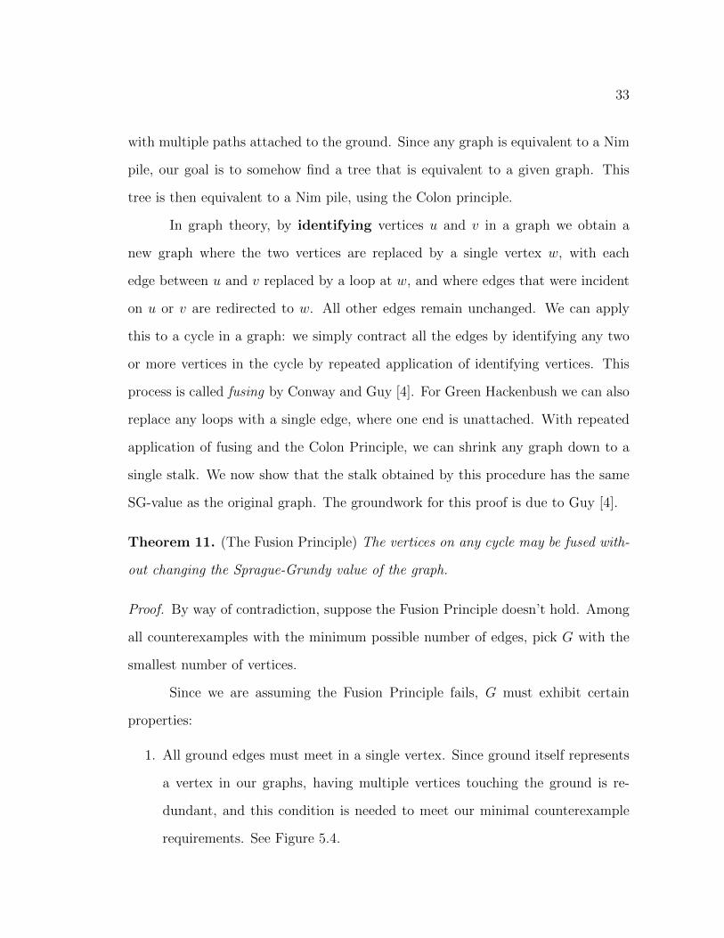
1. All ground edges must meet in a single vertex. Since ground itself represents

a vertex in our graphs, having multiple vertices touching the ground is re-

dundant, and this condition is needed to meet our minimal counterexample

requirements. See Figure 5.4.

34

Figure 5.4: All ground nodes must meet in a single vertex. These two graphsare equivalent, but the one on the right contains an extra vertex which vio-lates the way we defined the minimal counterexample. ighklghlkghklhlkjhklhklh-lkhlkhjlkhlkhjlkhjlkhlkhlkhkllhkhjlkhlkjhlkjh

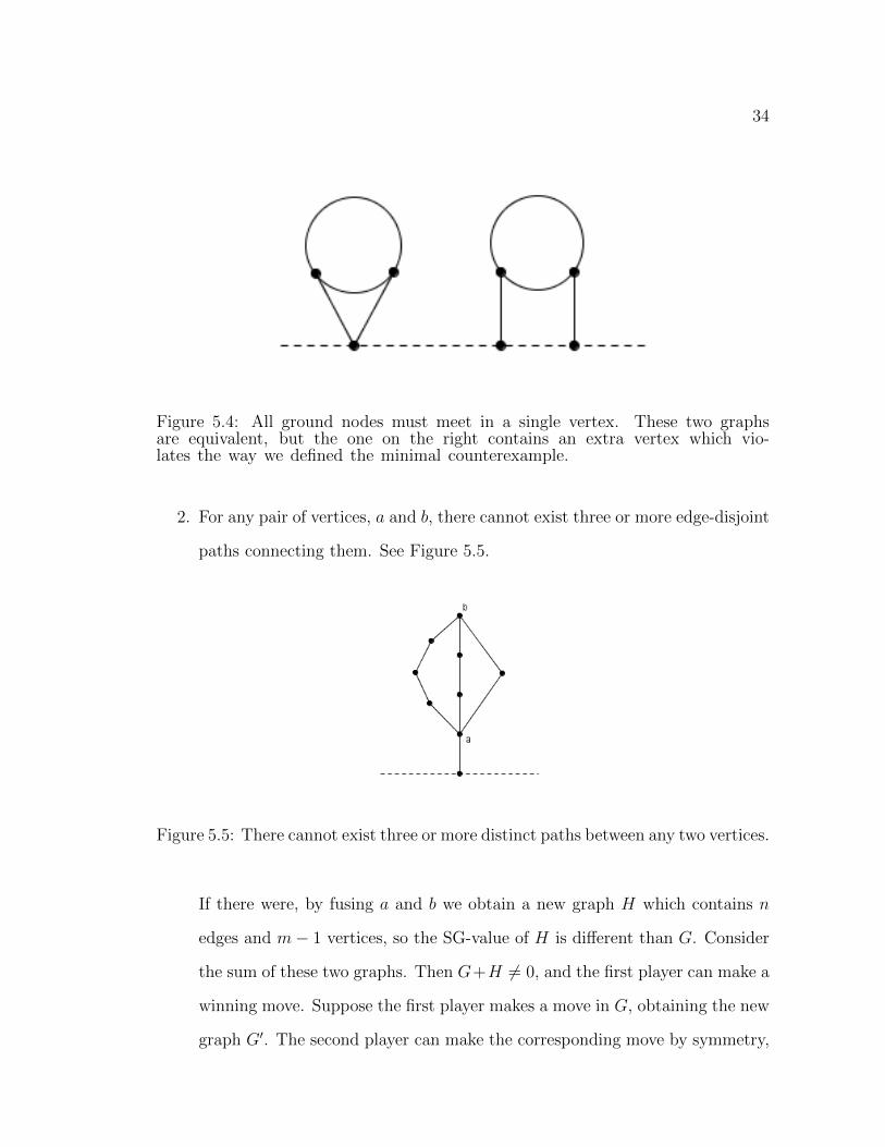
2. For any pair of vertices, a and b, there cannot exist three or more edge-disjoint

paths connecting them. See Figure 5.5.

Figure 5.5: There cannot exist three or more distinct paths between any two vertices.kjhlkhjkhlkhkhhlkhlkhkhlkhkhjlkhkhlkhlkhlkjhlkhjlkhlkhlkh

If there were, by fusing a and b we obtain a new graph H which contains n

edges and m− 1 vertices, so the SG-value of H is different than G. Consider

the sum of these two graphs. Then G+H 6= 0, and the first player can make a

winning move. Suppose the first player makes a move in G, obtaining the new

graph G′. The second player can make the corresponding move by symmetry,

35

removing the same edge in H, to obtain H ′. The same is true if the first

player makes a move in H to obtain H ′, as the second player can respond by

symmetry.

Now both G′ and H ′ have at most n− 1 edges, and we can apply the Fusion

Principle on each. But, since a and b were connected by three or more edge-

disjoint paths in G, the first player could have removed at most one of those

paths by removing an edge, so a and b are still on a cycle C in G′. Therefore,

after fusing C in G′ and the corresponding vertices, we obtain two identical

graphs, and G′ +H ′ = 0, which contradicts our assumption.

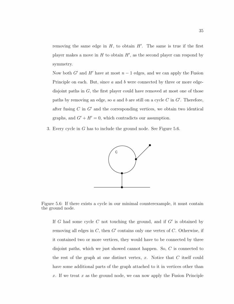
3. Every cycle in G has to include the ground node. See Figure 5.6.

Figure 5.6: If there exists a cycle in our minimal counterexample, it must containthe ground node. hlkjhkhlkhjlkhkljhlkhlkjhlkjhlkjhlkjhlkjhlkhlkjhlkjhlkjhlkhjk

If G had some cycle C not touching the ground, and if G′ is obtained by

removing all edges in C, then G′ contains only one vertex of C. Otherwise, if

it contained two or more vertices, they would have to be connected by three

disjoint paths, which we just showed cannot happen. So, C is connected to

the rest of the graph at one distinct vertex, x. Notice that C itself could

have some additional parts of the graph attached to it in vertices other than

x. If we treat x as the ground node, we can now apply the Fusion Principle

36

on the subgraph that includes C obtaining a graph C ′ with the same SG-

value. We can replace the original subgraph that contains C with C ′ and the

value of the original graph remains unchanged. The new graph is no longer a

counterexample.

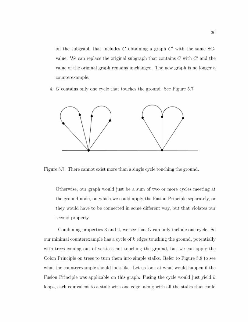
4. G contains only one cycle that touches the ground. See Figure 5.7.

Figure 5.7: There cannot exist more than a single cycle touching the ground. khlkjh-lkhklhkljhlkhjkljhlkhjlkhkljhlkhklhlkhlkhlkhlhlkjhklkh

Otherwise, our graph would just be a sum of two or more cycles meeting at

the ground node, on which we could apply the Fusion Principle separately, or

they would have to be connected in some different way, but that violates our

second property.

Combining properties 3 and 4, we see that G can only include one cycle. So

our minimal counterexample has a cycle of k edges touching the ground, potentially

with trees coming out of vertices not touching the ground, but we can apply the

Colon Principle on trees to turn them into simple stalks. Refer to Figure 5.8 to see

what the counterexample should look like. Let us look at what would happen if the

Fusion Principle was applicable on this graph. Fusing the cycle would just yield k

loops, each equivalent to a stalk with one edge, along with all the stalks that could

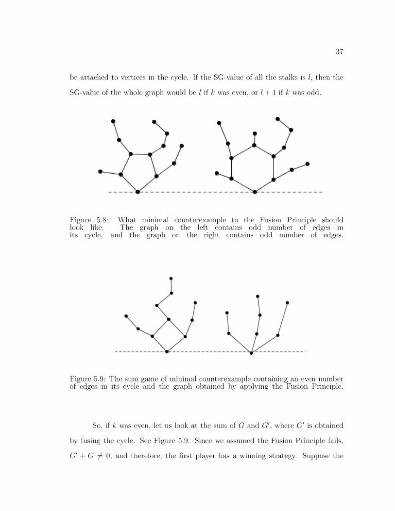
37

be attached to vertices in the cycle. If the SG-value of all the stalks is l, then the

SG-value of the whole graph would be l if k was even, or l + 1 if k was odd.

Figure 5.8: What minimal counterexample to the Fusion Principle shouldlook like. The graph on the left contains odd number of edges inits cycle, and the graph on the right contains odd number of edges.jlklj;lkj;lkj;lj;lj;lkjlj;jl;kjkjlkjlj;lkj;lj;kj;kj;lj;ljkl;kj;lkj;lkj;lj;l;lk

Figure 5.9: The sum game of minimal counterexample containing an even numberof edges in its cycle and the graph obtained by applying the Fusion Principle.gfsdhgf dghfdgh fdghdhgd ghfdgfdgh fdghfd ghfdgh fdhgfdg hfdhg hfdhgfd ghfdhgfdhgdhgdhgd

So, if k was even, let us look at the sum of G and G′, where G′ is obtained

by fusing the cycle. See Figure 5.9. Since we assumed the Fusion Principle fails,

G′ + G 6= 0, and therefore, the first player has a winning strategy. Suppose the

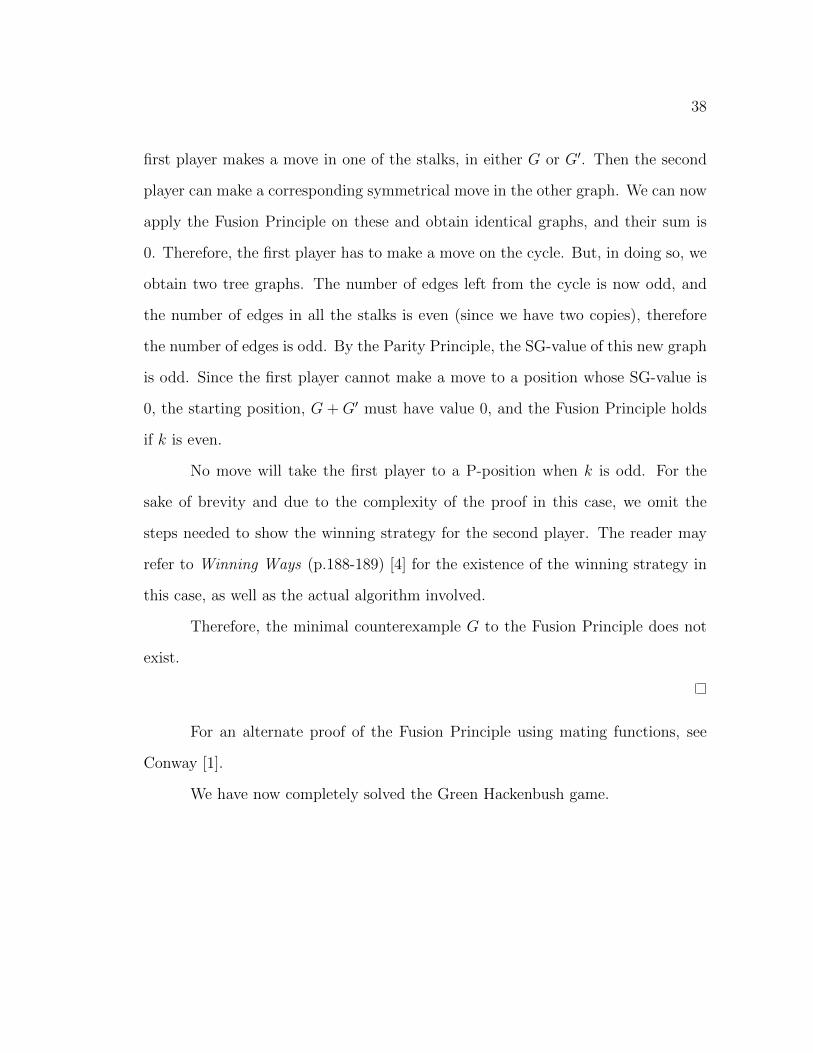
38

first player makes a move in one of the stalks, in either G or G′. Then the second

player can make a corresponding symmetrical move in the other graph. We can now

apply the Fusion Principle on these and obtain identical graphs, and their sum is

0. Therefore, the first player has to make a move on the cycle. But, in doing so, we

obtain two tree graphs. The number of edges left from the cycle is now odd, and

the number of edges in all the stalks is even (since we have two copies), therefore

the number of edges is odd. By the Parity Principle, the SG-value of this new graph

is odd. Since the first player cannot make a move to a position whose SG-value is

0, the starting position, G + G′ must have value 0, and the Fusion Principle holds

if k is even.

No move will take the first player to a P-position when k is odd. For the

sake of brevity and due to the complexity of the proof in this case, we omit the

steps needed to show the winning strategy for the second player. The reader may

refer to Winning Ways (p.188-189) [4] for the existence of the winning strategy in

this case, as well as the actual algorithm involved.

Therefore, the minimal counterexample G to the Fusion Principle does not

exist.

For an alternate proof of the Fusion Principle using mating functions, see

Conway [1].

We have now completely solved the Green Hackenbush game.

39

CHAPTER VI

CONCLUSION

We have analyzed Nim, Wythoff’s Nim, Moore’s Nim, Green Hackenbush,

and the misere versions for some of these. The characteristic properties of P and

N-positions and the Sprague-Grundy Function provided the groundwork that allows

us to analyze these games. In some cases we could determine which player has a

guaranteed win, even if we did not know what the winning strategy is.

The games we chose to study illustrated a number of different proof methods.

In Wythoff’s Nim, for example, we defined two sequences and then showed that

they span the P-positions. Also, the Golden ratio φ miraculously came up in the

discussion for generating the P-positions. In Green Hackenbush, we were able to

establish a few tools to reduce complicated positions to regular Nim, which we can

solve.

40

BIBLIOGRAPHY

[1] Conway J. (1976) On Numbers and Games. Academic Press, London.

[2] Ferguson T. (2008) Game Theory. University of California, Los Angeles. Web(http://www.math.ucla.edu/∼tom/Game Theory/Contents.html).

[3] Grundy P. M., (1939). Mathematics and games. Eureka 2: 68. Reprinted, 1964,27: 911.

[4] Guy R., Conway J., and Berlekamp E. (1982) Winning Ways for your mathe-matical plays, Volume I. Academic Press, London.

[5] Moore E. H., (1909) A generalization of the game called nim. Ann. of Math.(Ser. 2), 11:9394.

[6] Peres Y., with contributions by Wilson D., (2009) Game Theory, Alive. Uni-versity of California, Berkeley. Web. (http://dbwilson.com/games).

[7] Sprague R. P., (1935). Uber mathematische Kampfspiele. Tohoku MathematicalJournal 41: 438444.

[8] Wythoff W. A., (1907) A modification of the game of Nim. Nieuw Arch.Wisk.,7:199202.