Standard Operating Procedures for Converting Geologic Maps to GIS with ArcScan Extension in ArcMap 10.3

USGS Astrogeology Science Center

MRCTR GIS Lab

Flagstaff, AZ

Last Revised: 04/21/2017

MRCTR GIS LAB

2

PURPOSE

Planetary geologic maps created before the use of software such as Adobe Illustrator and ArcGIS contain critical information based on previous mission data, but have been retained only on walls and in drawers due to the time-intensive process of digitizing and packaging for use in a GIS. Converting this large backlog of maps to GIS form, and beginning with ArcMap 10.3 the ArcScan extension now allows for a streamlined conversion workflow which automates much of the line work digitization, reducing a 20-40+ hour task to 4-10 hours. This SOP will detail the entire process of converting a scanned geologic map into a GIS package, complete with documentation, ready for public release.

NOTE: To enable the ArcScan extension an Advanced ArcGIS 10.3+ Desktop license is required.

Required systems/software

ArcGIS Desktop 10.3 Advanced License

Basic ArcGIS features used in this SOP

Editing

Layer Properties

Spatial Reference

Georeferencing

Creating and Editing Metadata

ArcScan Extension

Create GIS Project

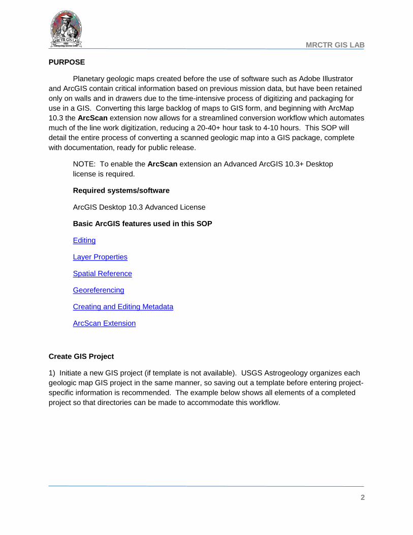
1) Initiate a new GIS project (if template is not available). USGS Astrogeology organizes each geologic map GIS project in the same manner, so saving out a template before entering project-specific information is recommended. The example below shows all elements of a completed project so that directories can be made to accommodate this workflow.

USGS ASTROGEOLOGY SCIENCE CENTER

3

ArcCatalog view of a completed GIS map conversion project.

Create Map Boundary, Spatial Reference & GDB

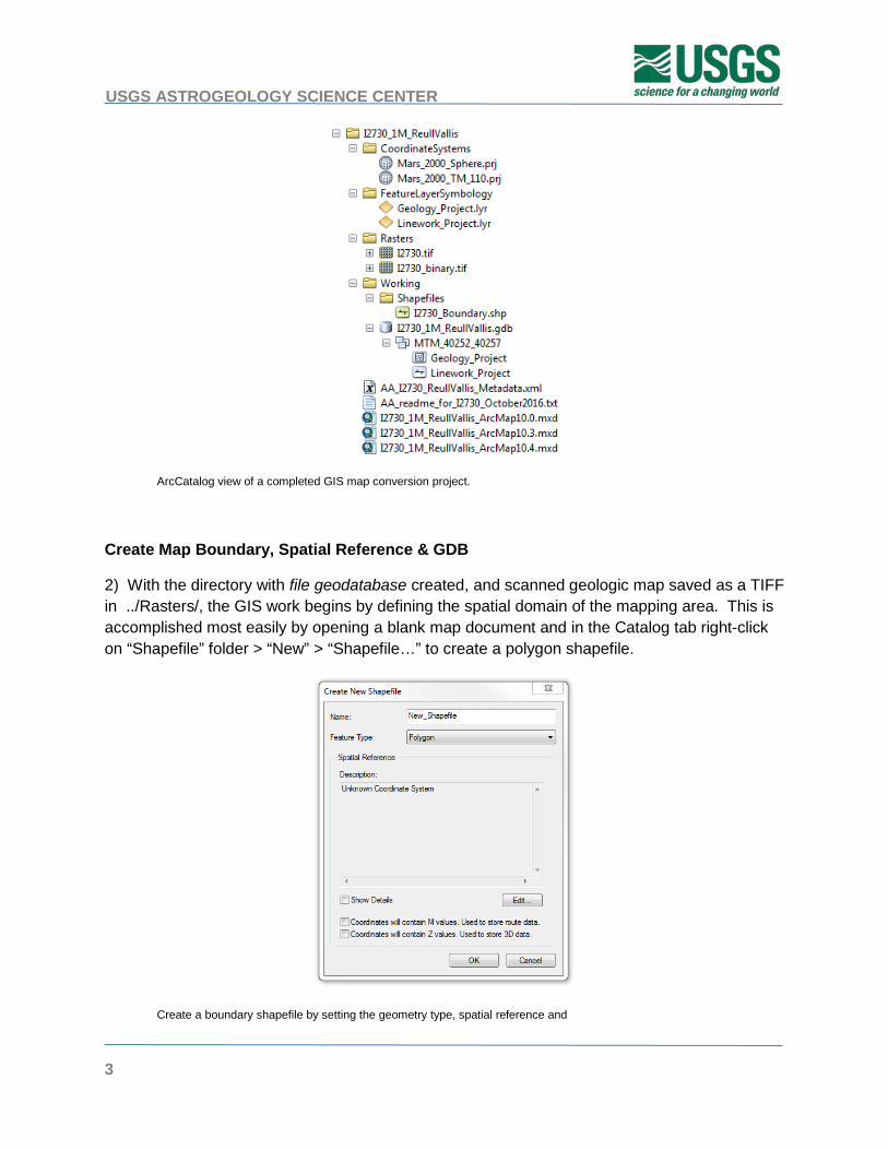
2) With the directory with file geodatabase created, and scanned geologic map saved as a TIFF in ../Rasters/, the GIS work begins by defining the spatial domain of the mapping area. This is accomplished most easily by opening a blank map document and in the Catalog tab right-click on “Shapefile” folder > “New” > “Shapefile…” to create a polygon shapefile.

Create a boundary shapefile by setting the geometry type, spatial reference and

MRCTR GIS LAB

4

Use the “Edit…” button in the Create New Shapefile dialog box to define the planetary body’s domain (Geographic Coordinate Systems (GCS) > Solar System > Planetary Body), then right-click and “Save As..” to export the projection file (*.prj) to the ../CoordinateSystems/ folder in your GIS map conversion project.

All spatial reference parameters can be modified by double-clicking the projection file.

If the required body radius is not available, then a new spherical or ellipsoidal body may be created by right-clicking the closest projection > “Copy and Modify” to modify the radius values of the major and minor axes to what you need.

Coordinate system Properties may be modified using existing projections and GCS’s.

USGS ASTROGEOLOGY SCIENCE CENTER

5

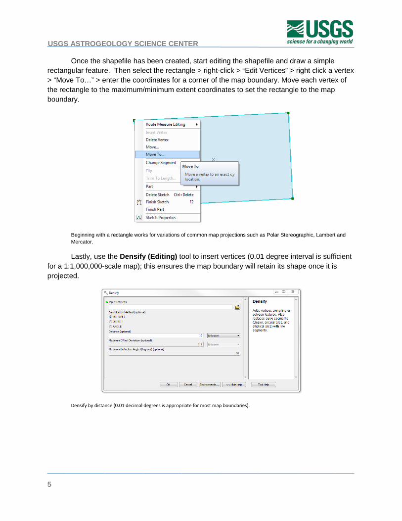
Once the shapefile has been created, start editing the shapefile and draw a simple rectangular feature. Then select the rectangle > right-click > “Edit Vertices” > right click a vertex > “Move To…” > enter the coordinates for a corner of the map boundary. Move each vertex of the rectangle to the maximum/minimum extent coordinates to set the rectangle to the map boundary.

Beginning with a rectangle works for variations of common map projections such as Polar Stereographic, Lambert and Mercator.

Lastly, use the Densify (Editing) tool to insert vertices (0.01 degree interval is sufficient for a 1:1,000,000-scale map); this ensures the map boundary will retain its shape once it is projected.

Densify by distance (0.01 decimal degrees is appropriate for most map boundaries).

MRCTR GIS LAB

6

Inserting vertices in coordinate space ensures the shape is maintained after projection.

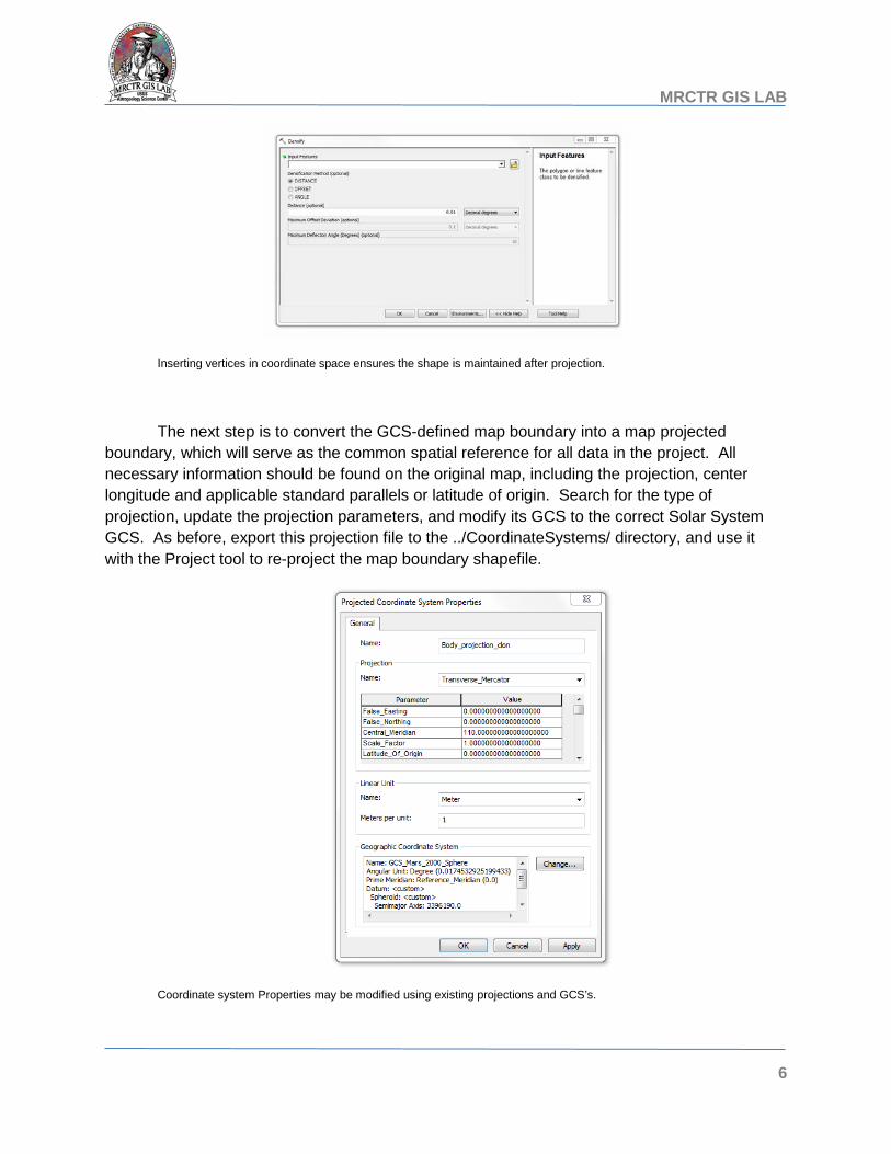
The next step is to convert the GCS-defined map boundary into a map projected boundary, which will serve as the common spatial reference for all data in the project. All necessary information should be found on the original map, including the projection, center longitude and applicable standard parallels or latitude of origin. Search for the type of projection, update the projection parameters, and modify its GCS to the correct Solar System GCS. As before, export this projection file to the ../CoordinateSystems/ directory, and use it with the Project tool to re-project the map boundary shapefile.

Coordinate system Properties may be modified using existing projections and GCS’s.

USGS ASTROGEOLOGY SCIENCE CENTER

7

Lastly, complete the geodatabase as necessary to support the project. Create a feature dataset with the spatial reference imported from the projected map boundary shapefile, and then create two polyline feature classes, one for contacts and one for structures (geologic units will be created later from finalized contacts). We strongly recommend using coded domains for all feature classes as they improve both the speed and accuracy of attribution.

Georeference Digital Map

3) Open a blank map document and bring in all elements created thus far (shapefile and feature classes). Then bring in the geologic map raster, and save the map document in the root of your project directory (ensure relative pathnames are used). Open the Georeferencing toolbar, and use control points to tie the corners of the digital map to the corners of the map boundary shapefile. Since the map boundaries are identical in shape a simple affine transformation should result in proper alignment of the entire map boundary. Then save the updated georeferencing to the raster. It is recommended that the ‘link file’ be saved with other supporting documentation for the project.

Georeferencing the digitized map to the projected map boundary should require only a simple affine transformation.

NOTE: If the map is to be georeferenced to a new base map (see renovation), many control points must be added throughout the map.

MRCTR GIS LAB

8

Convert RGB Image to Single-Band, Binary Raster

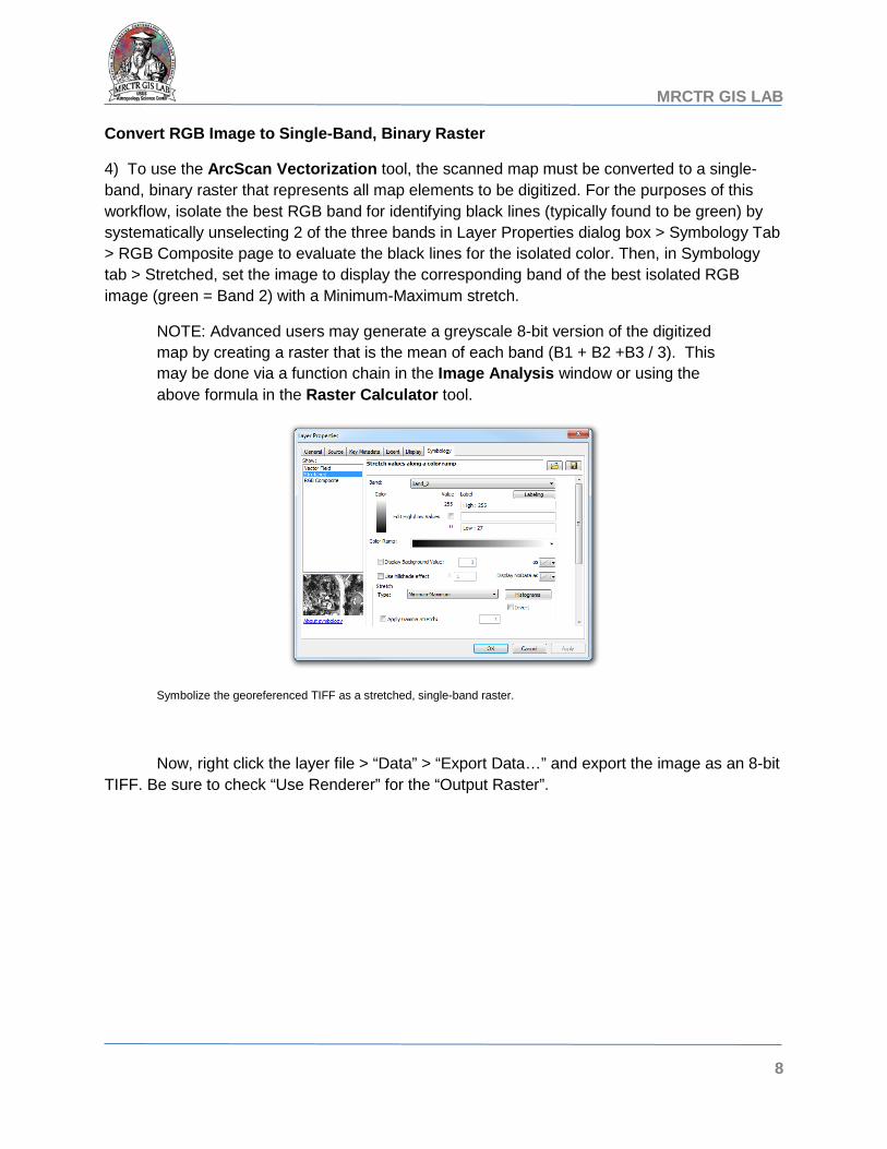
4) To use the ArcScan Vectorization tool, the scanned map must be converted to a single-band, binary raster that represents all map elements to be digitized. For the purposes of this workflow, isolate the best RGB band for identifying black lines (typically found to be green) by systematically unselecting 2 of the three bands in Layer Properties dialog box > Symbology Tab > RGB Composite page to evaluate the black lines for the isolated color. Then, in Symbology tab > Stretched, set the image to display the corresponding band of the best isolated RGB image (green = Band 2) with a Minimum-Maximum stretch.

NOTE: Advanced users may generate a greyscale 8-bit version of the digitized map by creating a raster that is the mean of each band (B1 + B2 +B3 / 3). This may be done via a function chain in the Image Analysis window or using the above formula in the Raster Calculator tool.

Symbolize the georeferenced TIFF as a stretched, single-band raster.

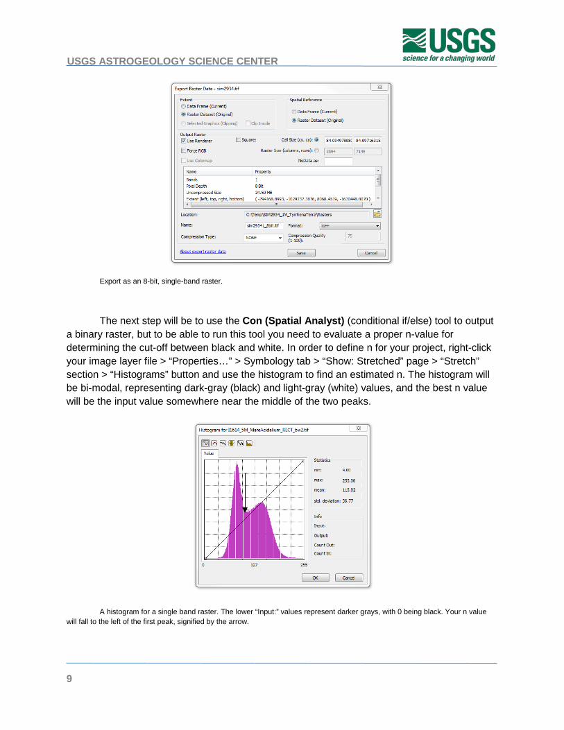
Now, right click the layer file > “Data” > “Export Data…” and export the image as an 8-bit TIFF. Be sure to check “Use Renderer” for the “Output Raster”.

USGS ASTROGEOLOGY SCIENCE CENTER

9

Export as an 8-bit, single-band raster.

The next step will be to use the Con (Spatial Analyst) (conditional if/else) tool to output a binary raster, but to be able to run this tool you need to evaluate a proper n-value for determining the cut-off between black and white. In order to define n for your project, right-click your image layer file > “Properties…” > Symbology tab > “Show: Stretched” page > “Stretch” section > “Histograms” button and use the histogram to find an estimated n. The histogram will be bi-modal, representing dark-gray (black) and light-gray (white) values, and the best n value will be the input value somewhere near the middle of the two peaks.

A histogram for a single band raster. The lower “Input:” values represent darker grays, with 0 being black. Your n value will fall to the left of the first peak, signified by the arrow.

MRCTR GIS LAB

10

Next, run the Con (Spatial Analyst) tool where all cells meeting the expression “VALUE <= n” return 1 (true) and all others return 0 (false). Save the output raster to ../Raster/ and symbolize it using unique values. This may require a few iterations to sample the best n for producing clean lines; if you sample pixels with the Identify tool, the value representing n will be the “Stretched value”.

Running the Con tool on a single-band image returns a binary raster for use in the ArcScan toolbar.

Lastly, the Majority Filter (Spatial Analyst) tool will be used to remove isolated pixels. Use the binary raster from the Con as input and the typical “Number of neighbors to use” is “FOUR” but you may run both “FOUR” and “EIGHT” to see which outputs a cleaner raster. It is important to note that whichever raster winds up being your final image to use for ArcScan needs to be set as binary: right-click image layer file > “Properties…” > Symbology tab > “Show:” Unique Values page. 0 and 1 should be shown as black and white, be sure “all other values” is unchecked.

The Majority Filter may not be necessary if the resolution of the scanned map is high quality.

USGS ASTROGEOLOGY SCIENCE CENTER

11

Set ArcScan Parameters

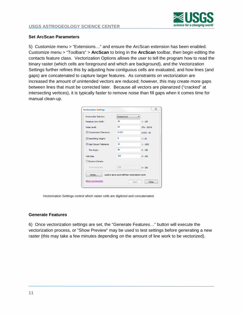
5) Customize menu > “Extensions…” and ensure the ArcScan extension has been enabled. Customize menu > “Toolbars” > ArcScan to bring in the ArcScan toolbar, then begin editing the contacts feature class. Vectorization Options allows the user to tell the program how to read the binary raster (which cells are foreground and which are background), and the Vectorization Settings further refines this by adjusting how contiguous cells are evaluated, and how lines (and gaps) are concatenated to capture larger features. As constraints on vectorization are increased the amount of unintended vectors are reduced; however, this may create more gaps between lines that must be corrected later. Because all vectors are planarized (“cracked” at intersecting vertices), it is typically faster to remove noise than fill gaps when it comes time for manual clean-up.

Vectorization Settings control which raster cells are digitized and concatenated.

Generate Features

6) Once vectorization settings are set, the “Generate Features…” button will execute the vectorization process, or “Show Preview” may be used to test settings before generating a new raster (this may take a few minutes depending on the amount of line work to be vectorized).

MRCTR GIS LAB

12

The input raster is converted to polylines, but large features may added to a polygon feature class.

Clean, Snap, Edit; Test & Correct Topology

7) Because the tool is meant to convert linear features there may be issues with how it reads polygons, such as gaps in coverage, large text and solid-fill symbology. Some of these issues may be overcome by refining parameters in Vectorization Settings, but there is rarely a 100% solution so some amount of manual editing is to be expected. Grid lines, text and other map elements not to be kept must first be deleted, and then features extended to fill any gaps, before quality control processing. This is the mostly lengthy process, and corrections to line work may still be made during the build polygons and topological testing steps.

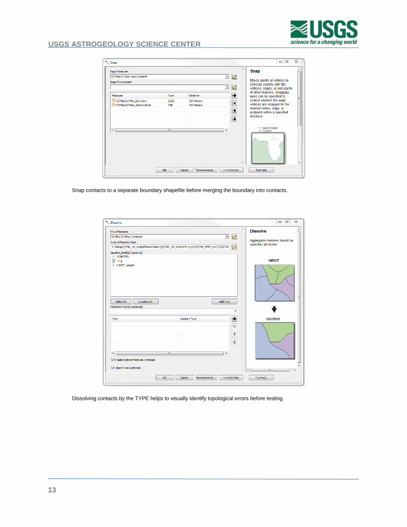
Before testing for topological errors, first run the contacts feature class through the Snap tool. Snapping tolerance should be at least the raster resolution or greater, and allow a greater snap tolerance for the boundary than itself. At this point the boundary may be merged with the contacts feature class, cleaned and attributed (the Extend and Trim tool in the Advanced Editing toolbar expedite this process). It is recommended to attribute all lines now as regular contacts or boundary, which helps with the Dissolve tool. Then run Dissolve based of the field TYPE. This will create a polyline feature class ready to test and validate using the Topology toolbar (for more information on Topology see this Esri reference.

USGS ASTROGEOLOGY SCIENCE CENTER

13

Snap contacts to a separate boundary shapefile before merging the boundary into contacts.

Dissolving contacts by the TYPE helps to visually identify topological errors before testing.

MRCTR GIS LAB

14

Smooth, Densify

8) The topologically intact polyline feature class will be accurate, but lack the smoothness of the original. To correct this effect run the Smooth Line tool, using the PAEK smoothing algorithm with a tolerance of at least the maximum offset found during sampling. Then use the Densify tool on the smoothed feature class; this will ensure polygons derived from these lines will retain their smooth shape.

The Smooth Line tool removes much of the jaggedness introduced by vectorization.

Densifying the smoothed lines ensures derived polygons retain their shape when projected.

USGS ASTROGEOLOGY SCIENCE CENTER

15

Attribute, Symbolize

9) With the line work completed, attribute by contact type, symbolize and save out the layer file to ../FeatureLayerSymbology/. For most purposes the “Geology 24K” contact symbols are equivalent to FGDC Chapter 25 Planetary Mapping Symbols.

Lines to Polygons

10) To convert the contacts feature class to geologic units run the Feature to Polygon tool, then attribute the polygons based on the original map (this is when coded domains are very useful). This polygon feature class can also be tested with the Topology toolbar; if errors are found, convert the polygon feature class to points (preserve attributes), correct the contacts, and build polygons again using the points to carry forward the unit attributes. As with the contacts, symbolize the polygons (sampling RGB values of the scanned map in Adobe Illustrator provides accurate recreation of unit symbols), and save out as a layer file.

Creating polygons from polylines can be an iterative process as errors are identified and corrected.

MRCTR GIS LAB

16

Document

11) All geologic maps converted to GIS should include documentation, including FGDC-standard metadata and a ReadMe file detailing all elements of the packaged project. ArcGIS supports the creation, transference and exporting of many metadata styles. Metadata is best created at the feature dataset level and then imported into each feature class.

Metadata can be edited, exported and imported in ArcCatalog using most format standards.

Package, Review

12) The final step is to remove all intermediate and redundant datasets in the project directory, rename files to match organizational standards, and prepare for distribution. It is good practice to test GIS projects on other machines, preferably with other versions of ArcMap as well.

Please direct any questions, comments or improvements to:

Marc Hunter

USGS Astrogeology Science Center

Flagstaff, AZ