Stochastic Choice and Consideration Sets∗

Paola Manzini Marco Mariotti†

This version: September 2013

Abstract

We model a boundedly rational agent who suffers from limited attention. The

agent considers each feasible alternative with a given (unobservable) probability,

the attention parameter, and then chooses the alternative that maximises a prefer-

ence relation within the set of considered alternatives. We show that this random

choice rule is the only one for which the impact of removing an alternative on the

choice probability of any other alternative is asymmetric and menu independent.

Both the preference relation and the attention parameters are identified uniquely

by stochastic choice data.

J.E.L. codes: D0.

Keywords: Discrete choice, Random utility, Logit model, Luce model, Considera-

tion sets, bounded rationality, revealed preferences.

∗We are grateful to three exceptionally thorough referees and the Co-Editor Wolfgang Pesendorfer for

many insightful suggestions and for correcting errors. We also thank various seminar audiences, as well

as Chris Flynn, Jacob Goeree, Sean Horan, Rosa Matzkin, Kemal Ozbek, Mauro Papi, Ivan Soraperra,

Rani Spiegler and Alex Tetenov for helpful comments on a previous related paper, “A salience theory of

choice errors" (IZA Discussion Paper No. 5006, 2010) in which the present paper originates. Financial

support from ESRC (grant ES/J012513/1) is gratefully acknowledged.†Both authors at School of Economics and Finance, University of St. Andrews, Castlecliffe, The

Scores, St. Andrews KY16 9AL, Scotland, U.K. (e-mail Manzini: paola.manzini@st-andrews.ac.uk; e-

mail Mariotti: marco.mariotti@st-andrews.ac.uk).

1

1 Introduction

We consider a boundedly rational agent who maximises a preference relation but makes

random choice errors due to imperfect attention. We extend the classical revealed pref-

erence method to this case of bounded rationality, and show how an observer of choice

frequencies can (1) test by means of simple axioms whether the data can have been gen-

erated by the model, and (2) if the answer to (1) is in the affi rmative, infer uniquely both

preferences and attention.

Most models of economic choice assume deterministic behaviour. Choice responses

are a function c that indicates the selection c (A) the agent makes from menu A. This

holds true both for the classical ‘rational’model of preference maximisation (Samuelson

[35], Richter [29]) and for more recent models of boundedly rational choice.1 Yet there is

a gap between such theories and real data, which are noisy: individual choice responses

typically exhibit variability, in both experimental and market settings (McFadden [27]).

We assume choice responses to be given by a probability distribution p that indicates

the probability p(a,A) that alternative a is selected from menu A, as in the pioneering

work of Luce [19], Block and Marschak’s [3] and Marschak’s [22], and more recently Gul,

Natenzon and Pesendorfer [15] (henceforth, GNP).

The source of choice errors in our model is the agent’s failure to consider all feasible

alternatives. For example, a consumer buying a new PC is not aware of all the latest

models and specifications;2 a time-pressured doctor overlooks the relevant disease for the

given set of symptoms; an ideological voter deliberately ignores some candidates indepen-

dently of their policies.3 In these examples the agent is able to evaluate the alternatives

he considers (unlike, for example, a consumer who is uncertain about the quality of a

product). Yet, for various reasons he does not rationally evaluate all objectively available

alternatives in A, but only a (possibly strict) subset of them, the consideration set C (A).

Once a C (A) has been formed, a final choice is made by maximising a preference relation

1The works on deterministic choice mentioned later constitute examples for this assertion.2Goeree [12] quantifies this phenomenon with empirical data.3Wilson [43] reports that African Americans tend to ignore Republican candidates in spite of the

overlap between their policy preferences and the stance of the Republicans, and even if they are dissatisfied

with the Democratic candidate.

2

over C (A), which we assume to be standard (complete and transitive).

This two-step conceptualisation of the act of choice is rooted in psychology and mar-

keting science, and it has recently gained prominence in economics through the works of

Masatlioglu, Nakajima and Ozbay [23] - (henceforth, MNO) - and Eliaz and Spiegler [9],

[10]. The core development in our model with respect to earlier works is that the compo-

sition of C (A) is stochastic. Each alternative a is considered with a probability γ (a), the

attention parameter relative to alternative a. For example, γ (a) may indirectly measure

the degree of brand awareness for a product, or the (complement of) the willingness of an

agent to seriously evaluate a political candidate. The assumption that γ (a) is menu inde-

pendent is a substantive one. It does have, however, empirical support in some contexts.4

And, at the theoretical level, the hypothesis of independent attention parameters is a

natural starting point. Unrestricted menu dependence yields a model with no observable

restrictions (Theorem 2), while it is not clear a priori what partial restrictions should be

imposed on menu dependence.

MNO’s [23] work is especially relevant for this paper as it is the first to study how

attention and preferences can be retrieved from choice data in a consideration set model

of choice. However, like in many other two-stage deterministic models of choice,5 it is not

possible in that model to pin down the primitives by observing the choice data that it

generates.6 An attractive feature of our approach is that it affords a unique identification

of the primitives. In particular, the preference for a over b is identified by the fact that

removing a from a menu containing b increases the probability that b is chosen (this change

in probability is called the impact of a on b). Our main result (Theorem 1) characterises

the model with two simple axioms, which state the asymmetry and menu independence

of the impacts.

The model can also be viewed as a special type of Random Utility Maximisation (see

section 7.1) and it rationalises some plausible types of choice mistakes that cannot be

captured by the Luce [19] rule (the leading type of restriction of Random Utility Max-

4See e.g. van Nierop et al [28].5E.g. our own “shortlisting" method Manzini and Mariotti [20].6We give an example in section 6. Tyson [41] clarifies the general structure of two-stage models of

choice.

3

imisation), in which p(a,A) = u (a) /∑b∈A

u (b) for some strictly positive utility function u.

The Luce rule is equivalent to the multinomial logit model (McFadden [26]) popular in

econometric studies, which assumes the maximisation of a random utility with additive

and Gumbel-distributed errors. This is a very specific error model and it is plausible to

conjecture that an agent may make different types of mistakes. The Luce rule is incompat-

ible, for example, with choice frequency reversals of the form p (a, {a, b, c}) > p (b, {a, b, c})

and p (b, {a, b}) > p (a, {a, b}). Because in our model the preference relation is asymmetric

but it is not revealed by crude choice probabilities, such reversals can be accommodated

(Example 1). Choice frequency reversals of various kinds have been observed experimen-

tally and they are natural when attention influences choice. For example, a superior but

unbranded cereal a may be chosen less frequently than a mediocre but branded cereal b,

simply because a is not considered. But if a third intermediate cereal c becomes available,

then b will be chosen less often (it will not be chosen whenever c is considered), while a

will be chosen with the same frequency as before, so that a reversal may occur. Similarly,

in spite of the transitivity of the underlying preference, the random consideration set

model is compatible with forms of stochastic intransitivity that are instead excluded by

Luce (section 4.2). Finally, a third important behavioural distinction from the Luce rule

concerns the well-known blue bus/red bus example (section 4.1).

2 Random choice rules

There is a nonempty finite set of alternatives X, and a domain D of subsets (the menus)

of X. We will assume that the domain satisfies the following ‘richness’ assumption:

{a, b, c} ∈ D for all distinct a, b, c ∈ X, and A ∈ D whenever B ∈ D and A ⊆ B. We

allow the agent not to pick any alternative from a menu, so we also assume the existence

of a default alternative a∗ (e.g. walking away from the shop, abstaining from voting,

exceeding the time limit for a move in a game of chess).7 Denote X∗ = X ∪ {a∗} and

A∗ = A ∪ {a∗} for all A ∈ D.7For a recent work on allowing ‘not choosing’in the deterministic case, see Gerasimou [11]. Earlier

work is Clark [6].

4

Definition 1 A random choice rule is a map p : X∗×D → [0, 1] such that:∑

a∈A∗ p (a,A) =

1 for all A ∈ D; p (a,A) = 0 for all a /∈ A∗; and p (a,A) ∈ (0, 1) for all a ∈ A∗, for all

A ∈ D\∅.

The interpretation is that p (a,A) denotes the probability that the alternative a ∈ A∗

is chosen when the possible choices (in addition to the default a∗) faced by the agent are

the alternatives in A. Note that a∗ is the action taken when the menu is empty, so that

p (a∗,∅) = 1.

We define a new type of random choice rule by assuming that the agent has a strict

preference ordering � on A. The preference � is applied only to a consideration set

C (A) ⊆ A of alternatives (the set of alternatives the decision maker pays attention to).

We allow for C (A) to be empty, in which case the agent picks the default option a∗, so

that p (a∗, A) is the probability that C (A) is empty. The membership of C (A) for the

alternatives in A is probabilistic. For all A ∈ D, each alternative a has a probability

γ (a) ∈ (0, 1) of being in C (A). Formally:

Definition 2 A random consideration set rule is a random choice rule p�,γ for which

there exists a pair (�, γ), where � is a strict total order on X and γ is a map γ : X →

(0, 1), such that8

p�,γ (a,A) = γ (a)∏

b∈A:b�a

(1− γ (b)) for all A ∈ D, for all a ∈ A

3 Characterisation

3.1 Revealed preference and revealed attention

Suppose the choice data are generated by a random consideration set rule. Can we

infer the preference ordering from the choice data? One way to extend the revealed

preference ordering of rational deterministic choice to stochastic choices is to declare

a � b iff p (a,A) > p (b, A) for some menu A (see GNP [15]). However, depending on

the underlying choice procedure, a higher choice frequency for a might not be due to a

genuine preference for a over b, and indeed this is not the way preferences are revealed in

8We use the convention that the product over the empty set is equal to one.

5

the random consideration set model. The discrepancy is due to the fact that an alternative

may be chosen more frequently than another in virtue of the attention paid to it as well

as of its ranking. We consider a different natural extension of the deterministic revealed

preference that accounts for this feature while retaining the same flavour as the standard

non stochastic environment.

In the deterministic case the preference for a over b has (among others) the observable

feature that b can turn from rejected to chosen when a is removed. This feature reveals

unambiguously that a is preferred to b, and has an analog in our random consideration

set framework. When a is ranked below b, there is no event in which the presence of a

in the consideration set matters for the choice of b; therefore if removing a increases the

choice probability of b, it means that a must be better ranked than b. And conversely if

a � b then excising a from A removes the event in which a is considered (in which case b is

not chosen), so that the probability of choosing b increases. Thus p (b, A\ {a}) > p (b, A)

defines the revealed preference relation a � b of our model. We will show that this relation

is revealed uniquely.9

Next, given a preference �, the attention paid to an alternative a is revealed directly

by the probability of choice in any menu in which a is the best alternative. For example

in Theorem 1 we admit all singleton menus, so that γ (a) = p (a, {a}) = 1 − p (a∗, {a}).

However γ (a) may be identified even when the choice probabilities from some menus

(singletons in particular) cannot be observed. Provided that there are at least three

alternatives and that binary menus are included in the domain, identification occurs via

the formula

γ (a) = 1−

√p (a∗, {a, b}) p (a∗, {a, c})

p (a∗, {b, c})

which must hold since under the model p (a∗, {b, c}) = (1− γ (b)) (1− γ (c)) and therefore

(1− γ (a))2 p (a∗, {b, c}) = (1− γ (a))2 [(1− γ (b)) (1− γ (c))]

= [(1− γ (a)) (1− γ (b))] [(1− γ (a)) (1− γ (c))]

= p (a∗, {a, b}) p (a∗, {a, c}) .9It is easy to see that p (a,A) = p (a,A\ {b}) also reveals the preference for a over b in our model

(again in analogy to rational deterministic choice).

6

This identification strategy can be further generalised using any disjoint menus B and

C instead of the alternatives b and c in the formula.10

These considerations suggest that the restrictions on observable choice data that char-

acterize the model are those ensuring that, firstly, the revealed preference relation � indi-

cated above is well-behaved, i.e. it is a strict total order on the alternatives; and, secondly,

that the observed choice probabilities are consistent with this � being maximised on the

consideration sets that are stochastically generated by the revealed attention parameters.

3.2 Axioms and characterisation theorem

Our axioms constrain the impactp (a,A\ {b})p (a,A)

that an alternative b ∈ A ∈ D has, in menu A, on another alternative a ∈ A∗ with a 6= b.

If p(a,A\{b})p(a,A)

> 1 we say that b boosts a and if p(a,A\{b})p(a,A)

= 1 that b is neutral for a. The

axioms are intended for all A,B ∈ D and for all a, b ∈ A ∩B, a 6= b.

i-Asymmetry. p(a,A\{b})p(a,A)

6= 1⇒ p(b,A\{a})p(b,A)

= 1.

i-Independence. p(a,A\{b})p(a,A)

= p(a,B\{b})p(a,B)

and p(a∗,A\{b})p(a∗,A) = p(a∗,B\{b})

p(a∗,B) .

i-Asymmetry says that if b is not neutral for a in a menu, then a must be neutral for

b in the same menu. Note how this axiom rules out randomness due to ‘utility errors’,

while it is compatible with ‘consideration errors’. It is a stochastic analog of a property

of rational deterministic choice: if the presence of b determines whether a is chosen, then

b is better than a, and therefore the presence of a cannot determine whether b is chosen.11

i-Independence states that the impact of an alternative on another cannot depend on

which other alternatives are present in the menu. It is a simple form of menu indepen-

dence, alternative to Luce’s IIA (Luce [19]):

Luce’s IIA. p(a,A)p(b,A)

= p(a,B)p(b,B)

.

10We thank two referees for suggesting these points.11On our specific domain, which contains singleton menus, i-Asymmetry could be weakened to

p(a,{a})p(a,{a,b}) 6= 1⇒

p(b,{b})p(b,{a,b}) = 1 thanks to i-Independence.

7

i-Independence is structurally similar to Luce’s IIA except that it relates to the impactsp(a,A\{b})p(a,A)

instead of the odd ratios p(a,A)p(b,A)

. These two properties appear to be equally

plausible ways to capture aspects of menu independence. If one thinks that preference

should be menu independent, then the a priori appeal of one or the other axiom hinges

on a hypothesis about what pattern reveals preference in the data. And, in turn, this

rests on a hypothesis on the cognitive process underlying choice. In the next section we

discuss further the relationship between the two properties.

A first interesting implication of the axioms (valid on any domain including all pairs

and their subsets) is instructive on how they act and will be used in the proof of the main

result:

i-Regularity. p(a,A\{b})p(a,A)

≥ 1 and p(a∗,A\{b})p(a∗,A) ≥ 1.

i-Regularity yields by iteration the standard axiom of Regularity (or Monotonicity),12

and says that if an alternative is not neutral for another alternative then it must boost it.

While it is often assumed directly, this is not a completely innocuous property: it excludes

for example the phenomenon of ‘asymmetric dominance’, whereby adding an alternative

that is clearly dominated by a but not by b increases the probability that a is chosen.

Lemma 1 If a random choice rule p satisfies i-Asymmetry and i-Independence then p

also satisfies i-Regularity.

Proof. Let p satisfy the assumptions in the statement. By i-Independence it is suffi cient

to show that p(a,{b})p(a,{a,b}) ≥ 1 and p(a∗,∅)

p(a∗,{a}) ≥ 1 for all a, b ∈ X. The latter inequality is

immediately seen to be satisfied since, by the definition of a random choice rule and of

a∗,p (a∗,∅)p (a∗, {a}) =

1

1− p (a, {a}) > 1

in view of p (a, {a}) ∈ (0, 1). Next, suppose by contradiction that there exist a, b ∈ X

12Regularity: A ⊂ B ⇒ p (a,A) ≥ p (a,B).

8

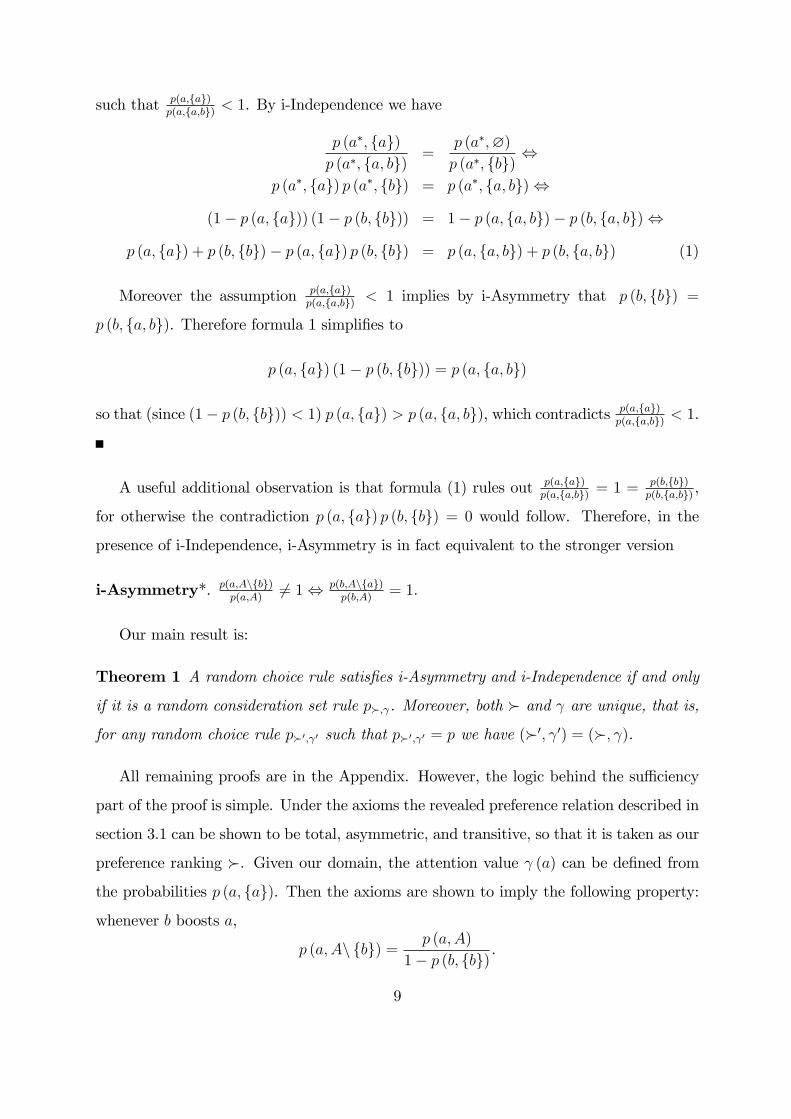
such that p(a,{a})p(a,{a,b}) < 1. By i-Independence we have

p (a∗, {a})p (a∗, {a, b}) =

p (a∗,∅)p (a∗, {b}) ⇔

p (a∗, {a}) p (a∗, {b}) = p (a∗, {a, b})⇔

(1− p (a, {a})) (1− p (b, {b})) = 1− p (a, {a, b})− p (b, {a, b})⇔

p (a, {a}) + p (b, {b})− p (a, {a}) p (b, {b}) = p (a, {a, b}) + p (b, {a, b}) (1)

Moreover the assumption p(a,{a})p(a,{a,b}) < 1 implies by i-Asymmetry that p (b, {b}) =

p (b, {a, b}). Therefore formula 1 simplifies to

p (a, {a}) (1− p (b, {b})) = p (a, {a, b})

so that (since (1− p (b, {b})) < 1) p (a, {a}) > p (a, {a, b}), which contradicts p(a,{a})p(a,{a,b}) < 1.

A useful additional observation is that formula (1) rules out p(a,{a})p(a,{a,b}) = 1 =

p(b,{b})p(b,{a,b}) ,

for otherwise the contradiction p (a, {a}) p (b, {b}) = 0 would follow. Therefore, in the

presence of i-Independence, i-Asymmetry is in fact equivalent to the stronger version

i-Asymmetry*. p(a,A\{b})p(a,A)

6= 1⇔ p(b,A\{a})p(b,A)

= 1.

Our main result is:

Theorem 1 A random choice rule satisfies i-Asymmetry and i-Independence if and only

if it is a random consideration set rule p�,γ. Moreover, both � and γ are unique, that is,

for any random choice rule p�′,γ′ such that p�′,γ′ = p we have (�′, γ′) = (�, γ).

All remaining proofs are in the Appendix. However, the logic behind the suffi ciency

part of the proof is simple. Under the axioms the revealed preference relation described in

section 3.1 can be shown to be total, asymmetric, and transitive, so that it is taken as our

preference ranking �. Given our domain, the attention value γ (a) can be defined from

the probabilities p (a, {a}). Then the axioms are shown to imply the following property:

whenever b boosts a,

p (a,A\ {b}) = p (a,A)

1− p (b, {b}) .

9

This is a weak property of ‘stochastic path independence’that may be of interest in

itself: it asserts that the boost of b on amust depend only on the ‘strength’of b in singleton

choice.13 Finally, the iterated application of this formula shows that the preference and

the attention parameters defined above retrieve in any menu the given choice probabilities

via the assumed procedure.

4 Explaining Menu effects and Stochastic Intransi-

tivity

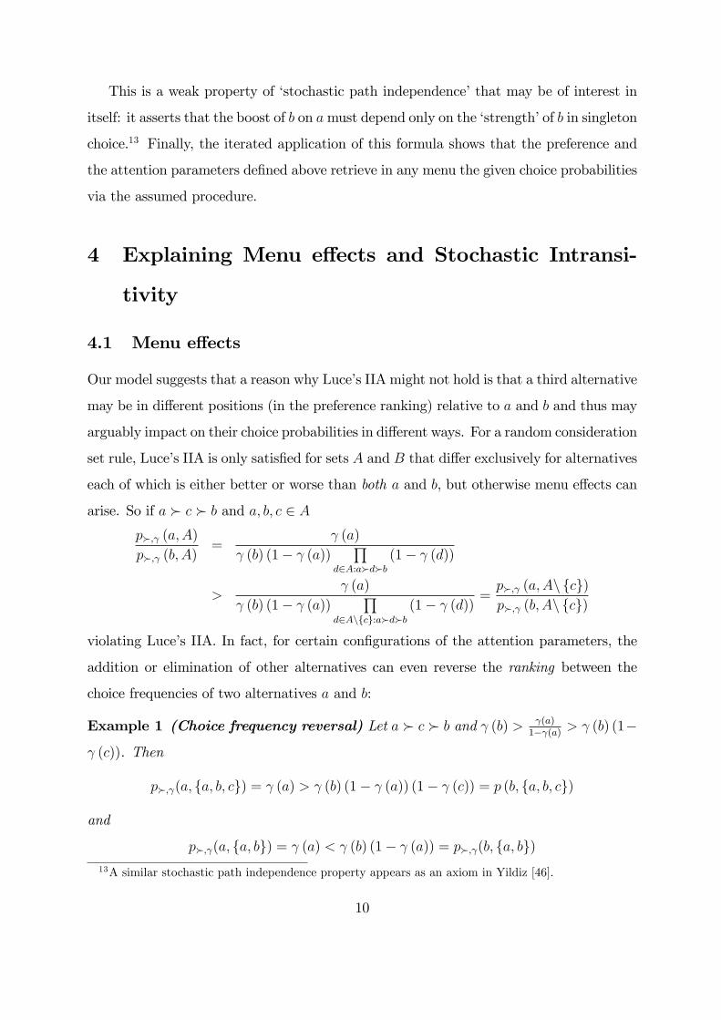
4.1 Menu effects

Our model suggests that a reason why Luce’s IIA might not hold is that a third alternative

may be in different positions (in the preference ranking) relative to a and b and thus may

arguably impact on their choice probabilities in different ways. For a random consideration

set rule, Luce’s IIA is only satisfied for sets A and B that differ exclusively for alternatives

each of which is either better or worse than both a and b, but otherwise menu effects can

arise. So if a � c � b and a, b, c ∈ Ap�,γ (a,A)

p�,γ (b, A)=

γ (a)

γ (b) (1− γ (a))∏

d∈A:a�d�b(1− γ (d))

>γ (a)

γ (b) (1− γ (a))∏

d∈A\{c}:a�d�b(1− γ (d)) =

p�,γ (a,A\ {c})p�,γ (b, A\ {c})

violating Luce’s IIA. In fact, for certain configurations of the attention parameters, the

addition or elimination of other alternatives can even reverse the ranking between the

choice frequencies of two alternatives a and b:

Example 1 (Choice frequency reversal) Let a � c � b and γ (b) > γ(a)1−γ(a) > γ (b) (1−

γ (c)). Then

p�,γ(a, {a, b, c}) = γ (a) > γ (b) (1− γ (a)) (1− γ (c)) = p (b, {a, b, c})

and

p�,γ(a, {a, b}) = γ (a) < γ (b) (1− γ (a)) = p�,γ(b, {a, b})13A similar stochastic path independence property appears as an axiom in Yildiz [46].

10

The basis for the choice frequency reversal in our model is that while a better alter-

native a may be chosen with lower probability than an inferior alternative b in pairwise

contests due to low attention for a, the presence of an alternative c that is better than

b but worse than a will reduce the probability that b is noticed without affecting the

probability that a is noticed, and possibly, if c attracts suffi ciently high-attention, to the

point that the initial choice probability ranking between a and b is reversed.14

However a random consideration set rule does satisfy other forms of menu inde-

pendence and consistency that look a priori as natural as Luce’s IIA. In addition to

i-Independence, it also satisfies, for all A ∈ D, a ∈ A∗ and b, c ∈ A:

i-Neutrality. p(a,A\{c})p(a,A)

, p(b,A\{c})p(b,A)

> 1⇒ p(a,A\{c})p(a,A)

= p(b,A\{c})p(b,A)

.

i-Neutrality states that an alternative has the same impact on any alternative in the

menu which it boosts. While an interesting property in itself, as it simplifies dramatically

the structure of impacts by forcing them to take on only a single value in addition to 1, this

is also a weakening of Luce’s IIA. In fact, i-Neutrality also states that p(a,A\{c})p(b,A\{c}) =

p(a,A)p(b,A)

under the boosting restriction in the premise (guaranteeing, in our interpretation, that c is

ranked above both a and b), while Luce’s IIA asserts the same form of menu independence

(and more) unconditionally. Our previous discussion explains why this restriction of

Luce’s IIA may be sensible.

The dependence of the choice odds on the other available alternatives is often a re-

alistic feature, which applied economist have sought to incorporate, for example, in the

multinomial logit model.15 The blue bus/red bus example (Debreu [7]) is the standard

illustration, in which menu effects occur because of an extreme ‘functional’similarity be-

tween two alternatives (a red and a blue bus). Suppose the agent chooses with equal

probabilities a train (t), a red bus (r) or a blue bus (b) as a means of transport in every

binary set, so that the choice probability ratios in pairwise choices for any two alternatives

are equal to 1. Then, on the premise that the agent does not care about the colour of the

14Choice frequency reversals of various nature have been observed experimentally. See e.g. Tsetsos,

Usher and Chater [37].15By adding a nested structure to the choice process (nested logit) or by allowing heteroscedasticity of

the choice errors (see e.g. Greene [13] or Agresti [1]). A probit model also allows for menu effects.

11

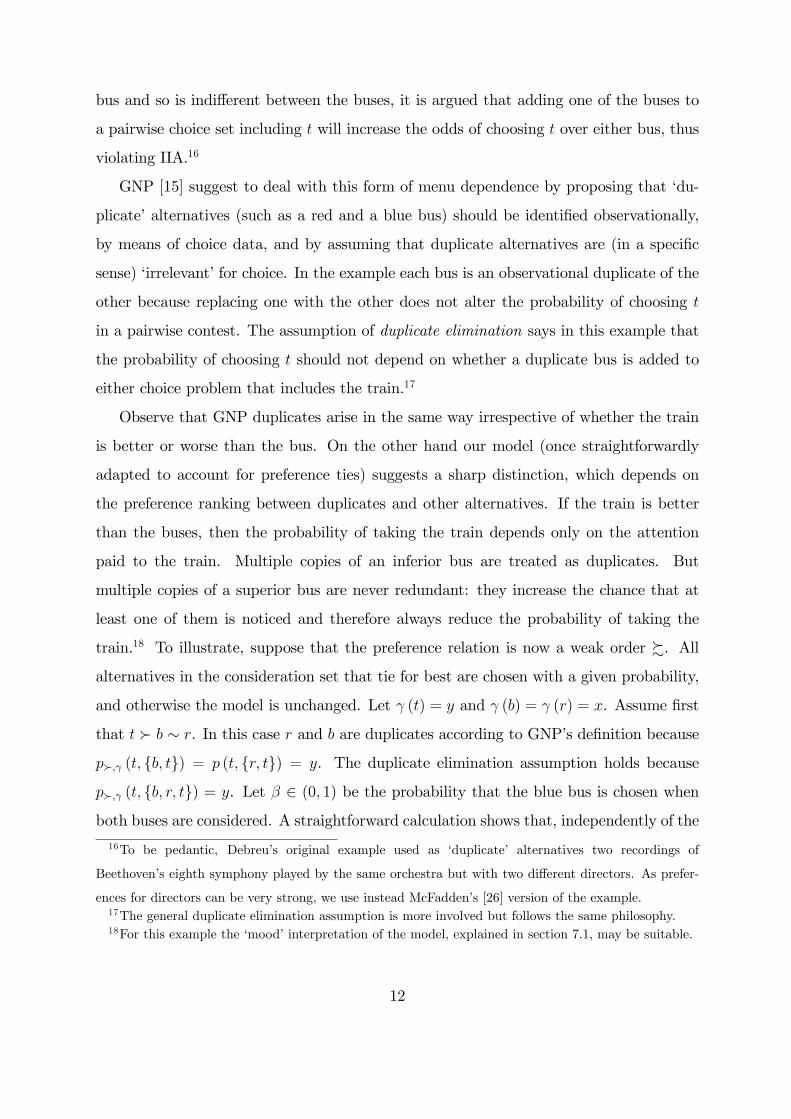
bus and so is indifferent between the buses, it is argued that adding one of the buses to

a pairwise choice set including t will increase the odds of choosing t over either bus, thus

violating IIA.16

GNP [15] suggest to deal with this form of menu dependence by proposing that ‘du-

plicate’alternatives (such as a red and a blue bus) should be identified observationally,

by means of choice data, and by assuming that duplicate alternatives are (in a specific

sense) ‘irrelevant’for choice. In the example each bus is an observational duplicate of the

other because replacing one with the other does not alter the probability of choosing t

in a pairwise contest. The assumption of duplicate elimination says in this example that

the probability of choosing t should not depend on whether a duplicate bus is added to

either choice problem that includes the train.17

Observe that GNP duplicates arise in the same way irrespective of whether the train

is better or worse than the bus. On the other hand our model (once straightforwardly

adapted to account for preference ties) suggests a sharp distinction, which depends on

the preference ranking between duplicates and other alternatives. If the train is better

than the buses, then the probability of taking the train depends only on the attention

paid to the train. Multiple copies of an inferior bus are treated as duplicates. But

multiple copies of a superior bus are never redundant: they increase the chance that at

least one of them is noticed and therefore always reduce the probability of taking the

train.18 To illustrate, suppose that the preference relation is now a weak order %. Allalternatives in the consideration set that tie for best are chosen with a given probability,

and otherwise the model is unchanged. Let γ (t) = y and γ (b) = γ (r) = x. Assume first

that t � b ∼ r. In this case r and b are duplicates according to GNP’s definition because

p�,γ (t, {b, t}) = p (t, {r, t}) = y. The duplicate elimination assumption holds because

p�,γ (t, {b, r, t}) = y. Let β ∈ (0, 1) be the probability that the blue bus is chosen when

both buses are considered. A straightforward calculation shows that, independently of the

16To be pedantic, Debreu’s original example used as ‘duplicate’ alternatives two recordings of

Beethoven’s eighth symphony played by the same orchestra but with two different directors. As prefer-

ences for directors can be very strong, we use instead McFadden’s [26] version of the example.17The general duplicate elimination assumption is more involved but follows the same philosophy.18For this example the ‘mood’interpretation of the model, explained in section 7.1, may be suitable.

12

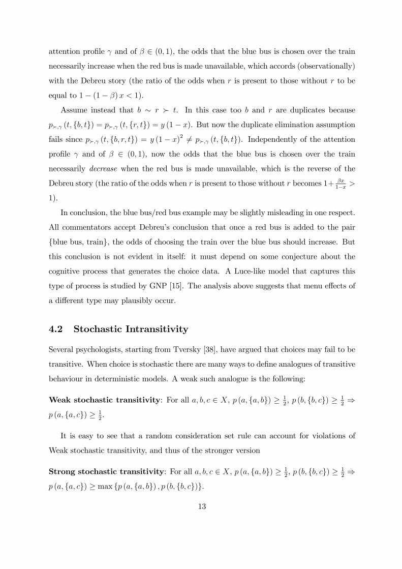
attention profile γ and of β ∈ (0, 1), the odds that the blue bus is chosen over the train

necessarily increase when the red bus is made unavailable, which accords (observationally)

with the Debreu story (the ratio of the odds when r is present to those without r to be

equal to 1− (1− β)x < 1).

Assume instead that b ∼ r � t. In this case too b and r are duplicates because

p�,γ (t, {b, t}) = p�,γ (t, {r, t}) = y (1− x). But now the duplicate elimination assumption

fails since p�,γ (t, {b, r, t}) = y (1− x)2 6= p�,γ (t, {b, t}). Independently of the attention

profile γ and of β ∈ (0, 1), now the odds that the blue bus is chosen over the train

necessarily decrease when the red bus is made unavailable, which is the reverse of the

Debreu story (the ratio of the odds when r is present to those without r becomes 1+ βx1−x >

1).

In conclusion, the blue bus/red bus example may be slightly misleading in one respect.

All commentators accept Debreu’s conclusion that once a red bus is added to the pair

{blue bus, train}, the odds of choosing the train over the blue bus should increase. But

this conclusion is not evident in itself: it must depend on some conjecture about the

cognitive process that generates the choice data. A Luce-like model that captures this

type of process is studied by GNP [15]. The analysis above suggests that menu effects of

a different type may plausibly occur.

4.2 Stochastic Intransitivity

Several psychologists, starting from Tversky [38], have argued that choices may fail to be

transitive. When choice is stochastic there are many ways to define analogues of transitive

behaviour in deterministic models. A weak such analogue is the following:

Weak stochastic transitivity: For all a, b, c ∈ X, p (a, {a, b}) ≥ 12, p (b, {b, c}) ≥ 1

2⇒

p (a, {a, c}) ≥ 12.

It is easy to see that a random consideration set rule can account for violations of

Weak stochastic transitivity, and thus of the stronger version

Strong stochastic transitivity: For all a, b, c ∈ X, p (a, {a, b}) ≥ 12, p (b, {b, c}) ≥ 1

2⇒

p (a, {a, c}) ≥ max {p (a, {a, b}) , p (b, {b, c})}.

13

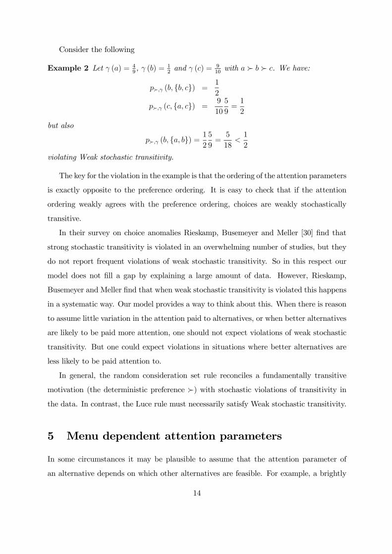
Consider the following

Example 2 Let γ (a) = 49, γ (b) = 1

2and γ (c) = 9

10with a � b � c. We have:

p�,γ (b, {b, c}) =1

2

p�,γ (c, {a, c}) =9

10

5

9=1

2

but also

p�,γ (b, {a, b}) =1

2

5

9=5

18<1

2

violating Weak stochastic transitivity.

The key for the violation in the example is that the ordering of the attention parameters

is exactly opposite to the preference ordering. It is easy to check that if the attention

ordering weakly agrees with the preference ordering, choices are weakly stochastically

transitive.

In their survey on choice anomalies Rieskamp, Busemeyer and Meller [30] find that

strong stochastic transitivity is violated in an overwhelming number of studies, but they

do not report frequent violations of weak stochastic transitivity. So in this respect our

model does not fill a gap by explaining a large amount of data. However, Rieskamp,

Busemeyer and Meller find that when weak stochastic transitivity is violated this happens

in a systematic way. Our model provides a way to think about this. When there is reason

to assume little variation in the attention paid to alternatives, or when better alternatives

are likely to be paid more attention, one should not expect violations of weak stochastic

transitivity. But one could expect violations in situations where better alternatives are

less likely to be paid attention to.

In general, the random consideration set rule reconciles a fundamentally transitive

motivation (the deterministic preference �) with stochastic violations of transitivity in

the data. In contrast, the Luce rule must necessarily satisfy Weak stochastic transitivity.

5 Menu dependent attention parameters

In some circumstances it may be plausible to assume that the attention parameter of

an alternative depends on which other alternatives are feasible. For example, a brightly

14

coloured object will stand out more in a menu whose other elements are all grey than in a

menu that only contains brightly coloured objects. In this section we show however that

a less restricted version of our model that allows for the menu dependence of attention

parameters is too permissive. A menu dependent random consideration set rule is a

random choice rule p�,δ for which there exists a pair (�, δ), where � is a strict total order

on X and δ is a map δ : X ×D\∅→ (0, 1), such that

p�,δ (a,A) = δ (a,A)∏

b∈A:b�a

(1− δ (b, A)) for all A ∈ D, for all a ∈ A

Theorem 2 For every strict total order � on X and for every random choice rule p,

there exists a menu dependent random consideration rule p�,δ such that p = p�,δ.

So, once we allow the attention parameters to be menu dependent, not only does the

model fail to place any observable restriction on choice data, but the preference relation

is also entirely unidentified. Strong assumptions on the function δ are needed to make

the model with menu dependent attention useful, but we find it diffi cult to determine

a priori what assumptions would be appropriate. The available empirical evidence on

brands suggests at best weak correlations between the probabilities of memberships of

the consideration set, and therefore weak menu effects.19

6 Related literature

The concept of consideration set originates in management science (Wright and Barbour

[44]).20 The economics papers that are most related to ours conceptually are MNO [23]

and Eliaz and Spiegler ([9], [10]). Exactly as in their models, an agent in our model who

chooses from menu A maximises a preference relation on a consideration set C (A). The

difference lies in the mechanism which determines C (A) (note that in the deterministic

case, without any restriction, this model is empirically vacuous, as one can simply declare

19For example van Nierop et al [28] estimate an unrestricted probabilistic model of consideration set

membership for product brands, and find that the covariance matrix of the stochastic disturbances to

the consideration set membership function can be taken to be diagonal.20See also Shocker, Ben-Akiva, Boccara and Nedungadi [36], Roberts and Lattin ([31],[32]) and Roberts

and Nedungadi [33].

15

the observed choice from A to be equal to C (A)). While Eliaz and Spiegler focus on

market competition and the strategic use of consideration sets, MNO focus on the direct

testable implications of the model and on the identification of the parameters. Our work

is thus more closely related to that of MNO. When the consideration set formation and

the choice data are deterministic as in MNO, consider a choice function c for which

c ({x, y}) = x = c ({x, y, z}), c ({y, z}) = y, c ({x, z}) = z. Then (as noted by MNO),

we cannot infer whether (i) x � z (in which case z is chosen over x in a pairwise contest

because x is not paid attention to) or (ii) z � x (in which case z is never paid attention

to in the larger set). The random consideration set model shows how richer data can

help break this type of indeterminacy. In case (i), the data would show that the choice

frequency of x is the same in {x, y, z} as in {x, y}. In case (ii), the data would show that

the choice frequency of x would be higher in {x, y} than in {x, y, z}.

We next focus on the relationship with models of stochastic choice.21

Tversky’s ([39], [40]) classical Elimination by Aspects (EBA) rule pε, which satisfies

Regularity, is such that there exists a real valued function U : 2X → <++ such that for

all A ∈ D, a ∈ A:

pε (a,A) =

∑B⊆X:B∩A 6=A U (B) pε (a,B ∩ A)∑

B⊆X:B∩A 6=∅ U (B)

There are random consideration set rules that are not EBA rules. Tversky showed that

for any three alternatives a, b, c EBA requires that if pε (a, {a, b}) ≥ 12and pε (b, {b, c}) ≥ 1

2,

then pε (a, {a, c}) ≥ min {pε (a, {a, b}) , pε (b, {b, c})} (Moderate stochastic transitivity).

Example 2 shows that this requirement is not always met by a random consideration set

rule.

Recently, GNP [15] have shown that, in a domain which is ‘rich’in a certain technical

sense, the Luce model is equivalent to the following Independence property (which is an or-

dinal version of Luce’s IIA): p (a,A ∪ C) ≥ p (b, B ∪ C) implies p (a,A ∪D) ≥ p (b, B ∪D)21Stochastic choice has also been used recently as a device in the literature of choice over menus. E.g.

Koida [18] studies how a decision maker’s (probabilistic) mental states drive the choice of an alternative

from each menu, in turn determining the agent’s preference for commitment in his choice over menus.

Ahn and Sarver [2] instead use the Gul and Pesendorfer’s [14] random expected utility model in the second

period of a menu choice model, and show how preference for flexibility yields a unique identification of

subjective state probabilities. In this paper we have focussed on choice from menus.

16

for all sets A,B,C and D such that (A ∪ B) ∩ (C ∪ D) = ∅. They also generalise the

Luce rule to the Attribute Rule in such a way as to accommodate red bus/blue bus type

of violations of Luce’s IIA (see section 4.1). We have seen that a random consideration

set rule violates one of the key axioms (duplicate elimination) for an Attribute Rule. And

the choice frequency reversal Example 1 violates the Independence property above.

Mattsson and Weibull [25] obtain an elegant foundation for (and generalisation of) the

Luce rule. In their model the agent (optimally) pays a cost to get close to implementing

any desired outcome (see also Voorneveld [42]). More precisely, the agent has to exert

more effort the more distant the desired probability distribution from a given default

distribution. When the agent makes an optimal trade-off between the expected payoff

and the cost of decision control, the resulting choice probabilities are a ‘distortion’ of

the logit model, in which the degree of distortion is governed by the default distribution.

Our paper shares with this work the broad methodology to focus on a detailed model

to explain choice errors. However, it is also very different in that Mattsson and Weibull

assume a (sophisticated form of) rational behaviour on the part of the agent. One may

then wonder whether ‘utility-maximisation errors’might not occur at the stage of making

optimal tradeoffs between utility and control costs, raising the need to model those errors.

A second major difference stems from the fact that our model uses purely ordinal pref-

erence information. Similar considerations apply to the recent wave of works on rational

inattention, such as Matejka and McKay [24], Cheremukhin, Popova and Tutino [5], and

Caplin and Dean [4], in which it is assumed that an agent solves the problem of allocating

attention optimally.

Recently, Rubinstein and Salant [34] have proposed a general framework to describe

an agent who expresses different preferences under different frames of choice. The link

with this paper is that the set of such preferences is interpreted as a set of deviations

from a true (welfare relevant) preference, so this is a model of ‘mistakes’. However, the

deviations are not analysed as stochastic events.

Finally, we note that the appeal of a two stage structure with a stochastic first stage

extends beyond economics, from psychology to consumer science. In philosophy in par-

ticular, it has been taken by some (e.g. James [17], Dennett [8], Heisenberg [16]) as a

17

fundamental feature of human choices, and as a solution of the general problem of free

will.

7 Concluding remarks22

7.1 Random consideration sets and RUM

A Random Utility Maximization (RUM) rule [3] is defined by a probability distribution π

on the possible rankings R of the alternatives and the assumption that the agent picks the

top element of the R extracted according to π. Block and Marschak [3], McFadden [26]

and Yellot [45] have shown that the Luce model is a particular case of a RUM rule, in which

a systematic utility is subject to additive random shocks that are Gumbel distributed. A

random consideration set rule (�, γ) is a different special type of RUM rule, in which π

is restricted as follows:

• π (R) = 0 for any ranking R for which there are alternatives a, b with a � b, bRa,

aRa∗ and bRa∗ (that is, if R contradicts � on some pair of alternatives, then at

least one of these alternatives must be R−inferior to a∗);

• for any alternative a, π ({R : aRa∗}) = γ (a) (that is, the probability of the set of

all rankings for which a is ranked above a∗ coincides with the probability that a is

noticed);

• for any two alternative a and b, π ({R : aRa∗ and bRa∗}) = γ (a) γ (b) (that is, the

events of any two alternatives being ranked above a∗ are independent).

For example, a random consideration set rule with two alternatives (beside the default)

such that γ (a) = 12, γ (b) = 1

3and a � b could be represented by the following RUM rule:23

π (aba∗) = 16, π (aa∗b) = 1

3, π (ba∗a) = 1

6, π (a∗ab) = π (a∗ba) = 1

6, π (baa∗) = 0.

An appealing interpretation of this type of RUM is that the agent is ‘in the mood’

for an alternative a with probability γ (a) (and otherwise prefers the default alternative),

22We thank the referees for suggesting most of the insights in this section.23Where a ranking is denoted by listing the alternatives from top to bottom.

18

and picks the preferred one among all alternatives for which he is in the mood. While

indistinguishable in terms of pure choice data, the RUM interpretation and the consider-

ation set interpretation imply different attitudes of the agent to ‘implementation errors’:

if a is chosen but b � a is implemented by mistake (e.g. a dish different from the one

ordered is served in a restaurant), the agent will have a positive reaction if he failed to

pay attention to b, but he will have a negative reaction if he was not in the mood for b.

7.2 Comparative attention

The model suggests a definition of comparative attention based on observed choice prob-

abilities. Say that (�1, γ1) is more attentive than (�2, γ2), denoted (�1, γ1)α (�2, γ2),

iff p�1,γ1 (a∗, A) < p�2,γ2 (a

∗, A) for all A ∈ D. Then we have that (�1, γ1)α (�2, γ2)

iff γ1 (a) > γ2 (a) for all a ∈ X (the ‘if’ direction follows immediately from the for-

mula p�,γ (a∗, A) =∏a∈A

(1− γ (a)), while the other direction follows from p�,γ (a∗, {a}) =

(1− γ (a)) applied to each {a} ∈ D). Observe that for two agents with the same pref-

erences, (�, γ1) is more attentive than (�, γ2) iff agent 1 makes ‘better choices’ from

each menu in the sense of first order stochastic dominance, that is p�,γ1 (a � b, A) >

p�,γ2 (a � b, A) for all b ∈ A with b 6= max (A,�), where p�,γ (a � b, A) denotes the

probability of choosing an alternative in A better than b.

On general domains (without the assumption that all singleton menus are included

in the domain) the implication (�1, γ1)α (�2, γ2) ⇒ γ1 (a) > γ2 (a) for all a ∈ X does

not necessarily hold. However, in a one-parameter version of the model in which all

alternatives receive the same attention g ∈ (0, 1), it follows from the formula p�,g (a∗, A) =

(1− g)|A| that (�1, g1)α (�2, g2) iff g1 > g2.

7.3 A model without default

A natural companion of our model that does not postulate a default alternative is one

in which whenever the agent misses all alternatives he is given the option to ‘reconsider’,

repeating the process until he notices some alternative. This leads to choice probabilities

19

of the form:

p�,γ (a,A) =

γ (a)∏

b∈A:b�a(1− γ (b))

1−∏b∈A(1− γ (b))

This model does not have the same identifiability properties as ours. For example,

take the case X = {a, b}, with p (a, {a, b}) = α and p (b, {a, b}) = β.24 These observations

(which fully identify the parameters in our model) are compatible with both the following

continua of possibilities:

• a � b and any γ such that γ(a)1−γ(a) =

αβγ (b);

• b � a and any γ such that γ(b)1−γ(b) =

βαγ (a).

Nevertheless, the model is interesting and it would be desirable to have an axiomatic

characterisation of it. We leave this as an open question.

References

[1] Agresti, A. (2002) Categorical Data Analysis, John Wiley and Sons, Hoboken, NJ.

[2] Ahn D. and T. Sarver (2013) “Preference for Flexibility and Random Choice”, Econo-

metrica 81: 341—361.

[3] Block, H.D. and J. Marschak (1960) “Random Orderings and Stochastic Theories

of Responses”, in Olkin, I., S. G. Gurye, W. Hoeffding, W. G. Madow, and H. B.

Mann (eds.) Contributions to Probability and Statistics, Stanford University Press,

Stanford, CA.

[4] Caplin, A. andM. Dean (2013) “Rational Inattention and State Dependent Stochastic

Choice”, mimeo, Brown University.

[5] Cheremukhin, A., A. Popova and A. Tutino (2011) “Experimental Evidence of Ra-

tional Inattention”, Working Paper 1112, Federal Reserve Bank of Dallas.

24Obviously in this model p (a, {a}) = 1 for all a ∈ X.

20

[6] Clark, S.A. (1995) “Indecisive choice theory”, Mathematical Social Sciences 30: 155-

170.

[7] Debreu, G., (1960) “Review of ‘Individual choice behaviour’by R. D. Luce"American

Economic Review 50: 186-88.

[8] Dennett, D. (1978) “On Giving Libertarians What They Say They Want", chapter

15 in Brainstorms: Philosophical Essays on Mind and Psychology, Bradford Books.

[9] Eliaz, K. and R. Spiegler (2011) “Consideration Sets and Competitive Marketing”,

Review of Economic Studies 78: 235-262.

[10] Eliaz, K. and R. Spiegler (2011) “On the strategic use of attention grabbers”, Theo-

retical Economics 6: 127—155.

[11] Gerasimou, G. (2010) “Incomplete Preferences and Rational Choice Avoidance”,

mimeo, University of St Andrews.

[12] Goeree, M. S. (2008) “Limited Information and Advertising in the US Personal Com-

puter Industry”, Econometrica 76: 1017-1074.

[13] Greene, W. H. (2003) “Econometric Analysis”, Prentice Hall, Upper Saddle River,

NJ.

[14] Gul, F. and W. Pesendorfer (2006) “Random Expected Utility”, Econometrica, 74:

121—146.

[15] Gul, F., P. Natenzon and W. Pesendorfer (2010) “Random Choice as Behavioral

Optimization”, mimeo, Princeton University.

[16] Heisenberg, M. (2009) “Is Free Will an Illusion?", Nature (459): 164-165.

[17] James, W. (1956) “The Dilemma of Determinism", in The Will to Believe and Other

Essays in Popular Philosophy (New York, Dover), p. 145-183.

[18] Koida, N. (2010) “Anticipated Stochastic Choice”, mimeo, Iwate Prefectural Univer-

sity.

21

[19] Luce, R. D. (1959) Individual Choice Behavior; a theoretical analysis. Wiley: New

York.

[20] Manzini, P. and M. Mariotti (2007) “Sequentially Rationalizable Choice”, American

Economic Review, 97 (5): 1824-1839.

[21] Manzini, P. and M. Mariotti (20XX) “Supplement to ‘Stochastic Choice

and Consideration Sets’",” Econometrica Supplemental Material, XX,

http://www.econometricsociety.org/ecta/supmat/XX.

[22] Marschak, J. (1960) “Binary choice constraints and random utility indicators”,

Cowles Foundation Paper 155.

[23] Masatlioglu, Y., D. Nakajima and E. Ozbay (2012): “Revealed Attention”, American

Economic Review, 102(5): 2183-2205

[24] Matejka, F. and A. McKay (2011) “Rational Inattention to Discrete Choices: A New

Foundation for the Multinomial Logit Model”, working paper 442 CERGE-EI.

[25] Mattsson, L.-G. and J. W. Weibull (2002) “Probabilistic choice and procedurally

bounded rationality”, Games and Economic Behavior, 41(1): 61-78.

[26] McFadden, D.L. (1974) “Conditional Logit Analysis of Qualitative Choice Behavior”,

in P. Zarembka (ed.), Frontiers in Econometrics, 105-142, Academic Press: New York.

[27] McFadden, D.L. (2000) “Economic choices”, American Economic Review, 91 (3):

351-378.

[28] van Nierop, E., B. Bronnenberg, R. Paap, M. Wedel & P.H. Franses (2010) “Re-

trieving Unobserved Consideration Sets from Household Panel Data", Journal of

Marketing Research XLVII: 63—74.

[29] Richter, M. K. (1966) “Revealed Preference Theory", Econometrica, 34: 635-645.

[30] Rieskamp, J., J.R. Busemeyer and B.A. Mellers (2006) “Extending the Bounds of

Rationality: Evidence and Theories of Preferential Choice" Journal of Economic

Literature 44: 631-661.

22

[31] Roberts, J. and Lattin (1991) “Development and testing of a model of consideration

set composition", Journal of Marketing Research, 28(4): 429—440.

[32] Roberts, J. H. and J. M. Lattin (1997) “Consideration: Review of research and

prospects for future insights" Journal of Marketing Research, 34(3): 406—410.

[33] Roberts, J. and P. Nedungadi, P. (1995) “Studying consideration in the consumer

decision process", International Journal of Research in Marketing, 12: 3—7.

[34] Rubinstein, A. and Y. Salant (2012) “Eliciting Welfare Preferences from Behavioral

Datasets”, Review of Economic Studies, 79, 375—387.

[35] Samuelson, P. A. (1938) “A Note on the Pure Theory of Consumer’s Behaviour”,

Economica, 5 (1): 61-71.

[36] Shocker, A. D., M. Ben-Akiva, B. Boccara and P. Nedungadi (1991) “Consideration

set influences on consumer decision-making and choice: Issues, models, and sugges-

tions" Marketing Letters, 2(3): 181—197.

[37] Tsetsos, K., M. Usher and N. Chater (2010) “Preference Reversal in Multiattribute

Choice”, Psychological Review 117: 1275—1293.

[38] Tversky, A. (1969) “Intransitivity of Preferences”Psychological Review, 76: 31-48.

[39] Tversky, A. (1972) “Choice by Elimination”, Journal of Mathematical Psychology 9:

341-67.

[40] Tversky, A. (1972) “Elimination by Aspects: A Theory of Choice”, Psychological

Review 79: 281-99.

[41] Tyson, C. J. (2011) “Behavioral Implications of Shortlisting Procedures”, forthcom-

ing in Social Choice and Welfare.

[42] Voorneveld, M. (2006) “Probabilistic choice in games: properties of Rosenthal’s t-

solutions”, International Journal of Game Theory 34: 105-121.

23

[43] Wilson, C. J. (2008) “Consideration Sets and Political Choices: A Heterogeneous

Model of Vote Choice and Sub-national Party Strength”, Political Behavior 30: 161—

183.

[44] Wright, P., and F. Barbour (1977) “Phased Decision Strategies: Sequels to an Initial

Screening.”In: Studies in Management Sciences, Multiple Criteria Decision Making,

ed. Martin K. Starr, and Milan Zeleny, 91-109, Amsterdam: North-Holland.

[45] Yellot, J.I., JR. (1977) “The relationship between Luce’s choice axiom, Thurstone’s

theory of comparative judgment, and the double exponential distribution”, Journal

of Mathematical Psychology, 15: 109-144.

[46] Yildiz, K. (2012) “List rationalizable choice”, mimeo, New York University.

Appendix A Proof of Theorem 1

The necessity part of the statement is immediately verified by checking the formula and

thus omitted here (see Manzini and Mariotti [21]). For suffi ciency, let p be a random

choice rule that satisfies i-Asymmetry and i-Independence. By Lemma 1 p also satisfies

i-Regularity, and by the observation after the proof of Lemma 1 it satisfies i-Asymmetry*

(below we will highlight where this stronger version of i-Asymmetry is needed). Define

a binary relation R on X by aRb iff p (b, A\ {a}) > p (b, A) for some A ∈ D, a, b ∈

A. We show that R is total, asymmetric and transitive. For totality, given a, b ∈ X,

suppose p (b, A\ {a}) ≤ p (b, A) for some A ∈ D (by the domain assumption there exists

an A ∈ D such that a, b ∈ A); then by i-Regularity p (b, A\ {a}) = p (b, A) and by i-

Asymmetry* p (a,A\ {b}) > p (a,A). For asymmetry, suppose p (b, A\ {a}) > p (b, A)

for some A ∈ D; then by i-Asymmetry p (a,A\ {b}) = p (a,A) and by i-Independence

p (a,B\ {b}) = p (a,B) for all B 3 a, b, B ∈ D.

For transitivity, it is convenient to introduce additional notation. For all A ∈ D and

for all a, b ∈ A, define xa = p (a, {a}) and λab = p(a,A)p(a,A\{b}) . By i-Independence λab is

well-defined. In particular for all a, b, c ∈ X we have (using the domain assumption)

p (a, {a, b, c})p (a, {a, c}) =

p (a, {a, b})p (a, {a}) = λab (2)

24

From (2) it follows that for all a, b, c ∈ X

p (a, {a, b}) = λabxa

(3)

p (a, {a, b, c}) = λacλabxa

Now fix any particular a, b, c ∈ X. By i-Independencep (a∗,∅)p (a∗, {a}) =

p (a∗, {b})p (a∗, {a, b}) =

p (a∗, {c})p (a∗, {a, c}) =

p (a∗, {b, c})p (a∗, {a, b, c})

which implies

p (a∗, {a, b}) = p (a∗, {b}) p (a∗, {a})

p (a∗, {a, b, c}) = p (a∗, {a}) p (a∗, {b, c}) = p (a∗, {a}) p (a∗, {b}) p (a∗, {c})

Since∑

a∈A∗ p (a,A) = 1, considering the menu {a, b, c} and all its binary subsets, using

(3) and writing p (a∗, {i}) as 1− xi, i ∈ {a, b, c} we have

λacλabxa + λbcλbaxb + λcaλcbxc + (1− xa) (1− xb) (1− xc) = 1

λabxa + λbaxb + (1− xa) (1− xb) = 1

λacxa + λcaxc + (1− xa) (1− xc) = 1

λbcxb + λcbxc + (1− xb) (1− xc) = 1

which can be rearranged, after expanding the products in (1− xi), as:

xaxb + xaxc + xbxc = (1− λacλab)xa + (1− λbcλba)xb + (1− λcaλcb)xc + xaxbxc

(1− λab)xa + (1− λba)xb = xaxb

(1− λac)xa + (1− λca)xc = xaxc

(1− λbc)xb + (1− λcb)xc = xbxc

Substitute the last three equations in the first one and rearrange to obtain

(1− λab) (1− λac)xa + (1− λba) (1− λbc)xb + (1− λca) (1− λcb)xc = xaxbxc (4)

Now suppose by contradiction that R is not transitive, that is let aRbRc and not (aRc).

Therefore λba > 1 and λcb > 1, and then by i-Asymmetry

λab = 1 = λbc

25

Moreover by totality cRa, i.e. there exists C ∈ D such that p (a, C\ {c}) > p (a, C) and

thus by i-Independence λac > 1, and then by i-Asymmetry

λca = 1

Substitute the values of λab, λbc and λca in equation (4) to obtain the contradiction

0 = xaxbxc > 0. We conclude that R is transitive.

Finally, concerning R, observe that (using i-Asymmetry* and i-Independence) the

following three statements are equivalent:

aRb

p (b, A\ {a}) > p (b, A) for all A ∈ D with a, b ∈ A

p (a,A\ {b}) = p (a,A) for all A ∈ D with a, b ∈ A (5)

Next, we show that for all A ∈ D, the following implication holds:

p (a,A\ {b}) > p (a,A)⇒ p (a,A\ {b})p (a,A)

=1

1− p (b, {b}) (6)

for all a ∈ A∗ and b ∈ A. We begin by proving (6) for a = a∗. Suppose first that A = {b}

for some b ∈ X. Since p (a∗,∅) = 1 and p (a∗, {b}) = 1− p (b, {b}), we have

p (a∗,∅)p (a∗, {b}) =

1

1− p (b, {b}) (7)

so that the assertion holds for this case. Then applying i-Independence to (7) we have

immediatelyp (a∗, A\ {b})p (a∗, {A}) =

1

1− p (b, {b})for all A ∈ D, for all b ∈ A. Next, fix a, b ∈ A and assume p (a,A\ {b}) > p (a,A), so that

by i-Asymmetry p (b, A\ {a}) = p (b, A). Using this equation and i-Independence yields

p (a,A\ {b})p (a,A)

=p (a, {a})p (a, {a, b}) =

1− p (a∗, {a})1− p (b, {a, b})− p (a∗, {a, b}) =

1− p (a∗, {a})1− p (b, {b})− p (a∗, {a, b})

and since as shown before

p (a∗, {a}) = p (a∗, {a, b})1− p (b, {b})

26

we havep (a,A\ {b})p (a,A)

=1− p(a∗,{a,b})

1−p(b,{b})

1− p (b, {b})− p (a∗, {a, b}) =1

1− p (b, {b})This concludes the proof that formula (6) holds.

Now define �= R and γ (a) = p (a, {a}) for all a ∈ X. We show that p�,γ = p. Fix

A ∈ D and number the alternatives so that A = {a1, ..., an} and ai � aj ⇔ i < j. For all

a ∈ A the implication in (6) and the definitions of γ and � imply that

p (ai, A) = p (ai, {a2, ..., an}) (1− γ (a1))...

= p (ai, {ai, ..., an})∏j<i

(1− γ (aj))

= p (ai, {ai})∏j<i

(1− γ (aj))

= γ (ai)∏j<i

(1− γ (aj)) = p�,γ (ai, A)

where p (ai, {ai}) = p (ai, {ai, ..., an}), which is used to move from the second to the third

line, follows from the properties of R in (5) (note that the probabilities in the display are

all well-defined by the domain assumption).

To conclude we show that � and γ are defined uniquely. Let p�′,γ′ be another consid-

eration set rule for which p�′,γ′ = p, and suppose by contradiction that �′ 6=�. So there

exist a, b ∈ X such that a � b and b �′ a. Take A = {a} ∪ {c ∈ X : a � c}, so that b ∈ A

for some b with b �′ a. By definition,

p�,γ (a,A) = γ (a) = p�,γ (a,B)

for all B ⊂ A such that a ∈ B, but also

p�′,γ′ (a,A) = γ′ (a)∏

c∈A:c�′a

(1− γ′ (c)) < γ′ (a)∏

c∈A\{b}:c�′a

(1− γ′ (c)) = p�′,γ′ (a,A\ {b})

a contradiction in view of p�′,γ′ = p = p�,γ. So � is unique. The uniqueness of γ is

immediate from p (a, {a}) = γ (a).

27

Appendix B Proof of Theorem 2

Let p be a random choice rule. Let � be an arbitrary strict total order of the alternatives.

Define δ by setting, for A ∈ D\∅ and a ∈ A:

δ (a,A) =p (a,A)

1−∑

b∈A:b�ap (b, A)

(8)

We have δ (a,A) > 0 since p (a,A) > 0, and we have δ (a,A) < 1 since 1 > p (a,A) +∑b∈A:b�a

p (b, A) (given that p (a∗, A) > 0).

For the rest of the proof fix a ∈ A. We define

p�,δ (a,A) = δ (a,A)∏

b∈A:b�a

(1− δ (b, A))

and show that p�,δ (a,A) = p (a,A). Using the definition of δ, for all b ∈ A we have

1− δ (b, A) =1−

∑c∈A:c�b

p (c, A)− p (b, A)

1−∑

c∈A:c�bp (c, A)

(9)

so that ∏b∈A:b�a

(1− δ (b, A)) =∏

b∈A:b�a

1−∑

c∈A:c�bp (c, A)− p (b, A)

1−∑

c∈A:c�bp (c, A)

(10)

Given any b ∈ A, denote by b+ ∈ A the unique alternative for which b+ � b and there

is no c ∈ A such that b+ � c � b. Letting b ∈ {c ∈ A : c � a}, from (9) we have that

1− δ(b+, A

)=

1−∑

c∈A:c�b+p (c, A)− p (b+, A)

1−∑

c∈A:c�b+p (c, A)

=

1−∑

c∈A:c�bp (c, A)

1−∑

c∈A:c�b+p (c, A)

As the numerator of the expression for 1 − δ (b+, A) is equal to the denominator of

the expression for 1− δ (b, A), the product in (10) is a telescoping product (where observe

that for the � −maximal term in A the denominator is equal to 1), and we thus have:∏b∈A:b�a

(1− δ (b, A)) = 1−∑

b∈A:b�a+p (b, A)− p

(a+, A

)= 1−

∑b∈A:b�a

p (b, A)

28

We conclude that

p�,δ (a,A) = δ (a,A)∏

b∈A:b�a

(1− δ (b, A))

=p (a,A)

1−∑

b∈A:b�ap (b, A)

(1−

∑b∈A:b�a

p (b, A)

)= p (a,A)

as desired (where the first term in the second line follows from (8)).

29