Stanford Exploration Project, Report 129, May 6, 2007 ...sep Exploration Project, Report 129, May 6, 2007, ... phase of the simulated primaries to the amplitude and ... where M is

Stanford Exploration Project, Report 129, May 6, 2007, pages 233–247

232

Stanford Exploration Project, Report 129, May 6, 2007, pages 233–247

Residual multiple attenuation using AVA modeling

Claudio Guerra

ABSTRACTResidual multiple attenuation is a common process applied towards the end of the seismicprocessing flow. Its main objective is to decrease the energy of migrated residual mul-tiples. This process can be time-consuming. I present a method which uses amplitude-versus-angle (AVA) modeling to simulate primary events and adaptive subtraction to es-timate residual multiples and residual-multiple-attenuated data. The method is appliedon angle-domain common-image gathers (ADCIGs) from a 2D data set from the Gulf ofMexico that is contaminated with residual multiples. This method is simple, fast and,depending on the parameterization of the adaptive subtraction, can preserve primary re-flection amplitudes.

INTRODUCTION

Conventional time and depth imaging considers that the input data is made up of only pri-mary reflections. Because of this basic assumption, much effort is spent attenuating eventsconsidered as noise. In the marine case, multiple reflections are the most important noise. Ifnot successfully attenuated, multiple reflections can bias velocity estimation, and after migra-tion, give rise to images contaminated with residual multiples which can make interpretationdifficult. For example, such contamination may severely interfere with AVA analysis.

In marine data processing, it is a common practice to run residual multiple attenuation asone of the later steps — after migration, for instance. The multiple-attenuation tests do notaccess every line of 3D data, and the evaluation of the efficacy of the attenuation is performedalong control lines. Since the multiple-attenuation parameters are optimized for the controllines, unfortunately, sometimes, a surprising amount of residual-multiple energy is left and isspread by migration over the entire migrated data set. Sometimes, the evaluation of the multi-ple attenuation is performed by inspecting post-stack migrated data, or even stacked volumes.Since this ignores the effect of pre-stack migration on the multiple-attenuated data, it canallow residual multiples to appear, manifesting as crosshatched patterns and high-frequencymigration noise resembling overmigrated events.

Another very common process after pre-stack migration is automatic residual-moveoutcorrection to mitigate the effects of velocity inaccuracies, which aims to align reflectors hor-izontally to improve the stacking power and better constrain the data for AVA analysis. Con-sequently, a method which relies on the flatness of the gathers is a natural process to attenu-

233

234 Guerra SEP–129

ate residual multiples after automatic residual-moveout correction. However, the problem ofresidual moveout will not be addressed in this work.

Weglein (1999) classified multiple-attenuation methods into two main categories: (1) fil-tering methods and (2) prediction methods. The most widely used filtering methods rely ondifferences in traveltime between primaries and multiples to separate them in appropriate do-mains where multiples can be filtered out (Hampson, 1987). Since, regardless of the domain,primaries and multiples normally overlap, particularly at small reflection angles and offsets,the filtering is not perfect; therefore, some of the primary energy can be attenuated, or someof the multiple energy is left out (crosstalk). Prediction methods simulate multiples by auto-convolution of shot gathers and then subtract them from the original data using nonlinearadaptive subtraction (Verschuur et al., 1992). As prediction methods became popular, filteringmethods inherited the nonlinear adaptive subtraction to attack the crosstalk problem. So, fil-tering methods can be used to estimate multiples by exploring the same differences betweenthem and primaries as before, but instead of simply filtering them out, a possible approach isto subtract the estimated multiples from the original data using nonlinear adaptive-subtractionschemes. This provides more flexibility to solve specific problems.

Generally, residual-multiple attenuation is performed by filtering methods, by zeroing theresidual-multiple energy (along with some primary energy) or by using nonlinear adaptivesubtraction. Choo et al. (2004) devised a method to perform residual-multiple attenuation ina different manner. They apply AVA inversion to simulate the primaries and then estimate theresidual multiples using nonlinear adaptive subtraction. Although many details of their workare unpublished, the method I present here is, in essence, very similar to the one proposed bythem. The method simulates the primaries according to an AVA curve, adjusts amplitude andphase of the simulated primaries to the amplitude and phase of the original data by applyingfilters computed in a nonlinear adaptive strategy, subtracts the adjusted primaries from theoriginal data to get an estimate of the residual multiples, and, finally, obtains the attenuateddata by nonlinear adaptive subtraction. This approach solves the AVA modeling problemglobally.

The method is applied on angle-domain common-image gathers (ADCIGs) of a Gulf ofMexico (GOM) 2D data subjected to multiple attenuation after migration. The data set con-tains very complex multiple patterns (Alvarez et al., 2004).

DESCRIPTION OF THE METHOD

Aki and Richards (1980) stated that, up to 40◦, the p-wave reflection coefficients, R(θ ), as afunction of the incidence angle, θ , can be approximated by

R(θ ) = A+ B sin2θ +C tan2

θ , (1)

where A, B and C are parameters related to the average and contrasts of the elastic properties ofthe limiting layers. Therefore, if it is possible to determine these parameters, one can simulatethe amplitudes of primary events at every depth or time step. I refer to the simulation of theprimary amplitudes as AVA modeling. The aim of this work is not to invert the AVA parameters

SEP–129 Residual multiple attenuation 235

for rock and fluid properties, but just to obtain a reasonable estimate of the primaries to befurther used in a residual-multiple-attenuation sequence.

The AVA modeling problem can be addressed by solving locally, for every different depth(or time) step, the normal equations (GTG)m = GTd, where m are the estimated AVA param-eters, G has the column vector form [1, sin2

θi, tan2θi] and d is the ADCIG (or a CMP gather

after NMO). The simulated primaries are obtained by using the estimated AVA parametersin equation (1). One problem that arises from this local solution is that the AVA parametersare not constrained to be smooth along depth. This can lead to anomalous amplitudes in thesimulated primaries for a certain depth.

In the present approach, the AVA modeling problem consists of determining the threeparameters A, B and C of equation (1) by solving the following data fitting problem:

Lm = d, (2)

where L in matrix form is

11 S1 T112 S2 T213 S3 T3... ... ...

1n1 Sn1 Tn1

(3)

which has dimension n1n2 × 3n1 , m is the model-parameter vector (3n1 elements), and d isthe data vector (n1n2 elements), where n1 and n2 are the number of samples in depth (or time)and the number of traces in the ADCIG, respectively. 1j , Sj and Tj are n2 × n1 matricesconsisting of 1, (sin2

θi ) and (tan2θi ) along their j-th column entries, respectively. i stands for

the reflection-angle indexes.

Generally, in ADCIGs, residual multiples are more persistent at near angles, because ofinsufficient moveout difference between them and the flattened primaries. Additionally, at thefarthest angles, stretch occurs. To avoid these imperfections in the input data, the fitting goalis to minimize the residual,

0 ≈ M(Lm−d), (4)

where M is a selector operator which applies the appropriate internal and external mutes.

If unrealistic variations of the AVA parameters with depth are an issue, the following reg-ularization goal can be introduced:

0 ≈ εDm, (5)

where D is the derivative operator along depth and ε is the regularization parameter. As usual,care must be taken when choosing ε not to destroy any recoverable residual moveout informa-tion and not to spread simulated primaries to angles at which they originally do not occur.


To accelerate the solution, the problem can be solved with preconditioning (Claerbout andFomel, 2001), using the transformation m = Cp, where C = D−1 and p is the preconditionedvariable. Finally, the fitting goals reduce to

0 ≈ M(LCp−d)0 ≈ εp. (6)

The final model is obtained with m = Cp. I use conjugate-gradients to solve the inverseproblem.

After the determination of the three AVA parameters for every depth step, primaries aresimulated by computing the reflection coefficient for all reflection angles using equation (1).Of course, the method relies on the flatness of the reflectors in the CIG to correctly extract the3 parameters of the AVA curve.

To get the residual-multiple-attenuated data, the adaptive subtraction must be applied intwo steps. The first one aims to obtain an estimate of the residual multiples. This is doneby subtracting the adjusted version of the simulated primaries from the original data. Ampli-tude and phase adjustments are achieved by the convolution of the simulated primaries with aprediction-error Wiener filter.

As the estimated residual multiples may contain some primary information (mainly atsmall reflection angles), I use the strategy proposed by Guitton et al. (2001), the so-called ‘sub-traction method,’ in which two different prediction-error filters (PEFs), which model primariesand multiples, are computed. Their method allows regularization, to decrease the crosstalk be-tween multiples and primaries. The corresponding fitting goals are

0 ≈ mn0 ≈ εms

subjected to ↔ d = S−1ms +N−1mn

after preconditioning, with s = S−1ms and n = N−1mn. In the preconditioning equations, srepresents the primaries, n the multiples; N−1 and S−1 represent deconvolution with PEFs formultiples and primaries, respectively; mn is the multiple model content and ms is the primarymodel content. Finally, the estimated primaries are obtained by s = d−N−1mn. All PEFs arecomputed with conjugate-gradients.

EXAMPLES

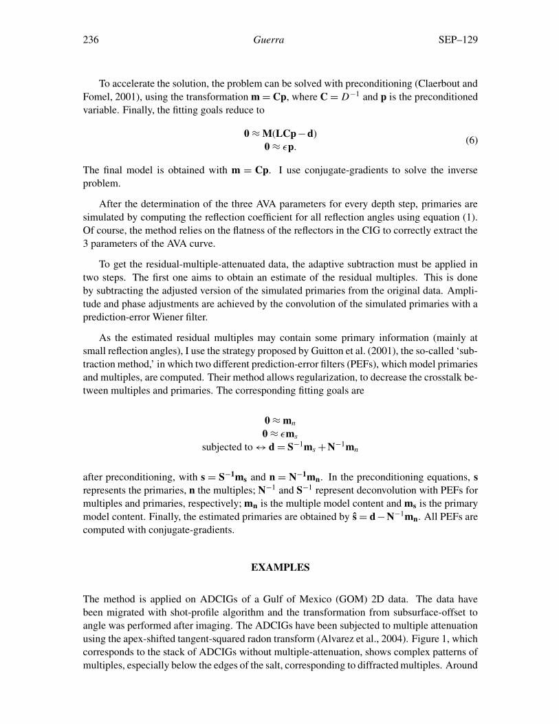
The method is applied on ADCIGs of a Gulf of Mexico (GOM) 2D data. The data havebeen migrated with shot-profile algorithm and the transformation from subsurface-offset toangle was performed after imaging. The ADCIGs have been subjected to multiple attenuationusing the apex-shifted tangent-squared radon transform (Alvarez et al., 2004). Figure 1, whichcorresponds to the stack of ADCIGs without multiple-attenuation, shows complex patterns ofmultiples, especially below the edges of the salt, corresponding to diffracted multiples. Around


a depth of 3500 m, the first-order multiple of the sea bottom is probably distorted due to thealternation between fast and slow velocities. The fitting goal I used to simulate the primariesis the one given in equation (6).

Figure 1: Migrated data without multiple attenuation – stacked data. Notice strong migratedmultiples, especially below the edges of the salt, corresponding to migrated diffracted multi-ples. claudio1-migstk [ER]

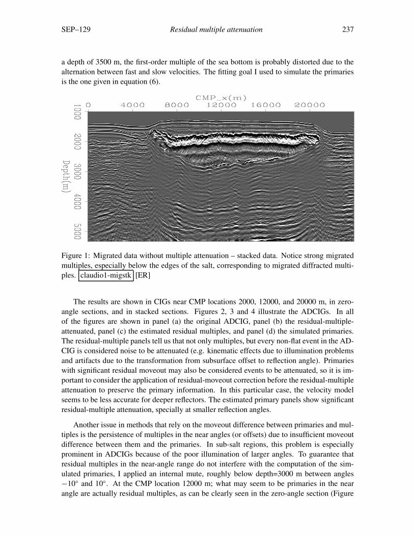
The results are shown in CIGs near CMP locations 2000, 12000, and 20000 m, in zero-angle sections, and in stacked sections. Figures 2, 3 and 4 illustrate the ADCIGs. In allof the figures are shown in panel (a) the original ADCIG, panel (b) the residual-multiple-attenuated, panel (c) the estimated residual multiples, and panel (d) the simulated primaries.The residual-multiple panels tell us that not only multiples, but every non-flat event in the AD-CIG is considered noise to be attenuated (e.g. kinematic effects due to illumination problemsand artifacts due to the transformation from subsurface offset to reflection angle). Primarieswith significant residual moveout may also be considered events to be attenuated, so it is im-portant to consider the application of residual-moveout correction before the residual-multipleattenuation to preserve the primary information. In this particular case, the velocity modelseems to be less accurate for deeper reflectors. The estimated primary panels show significantresidual-multiple attenuation, specially at smaller reflection angles.

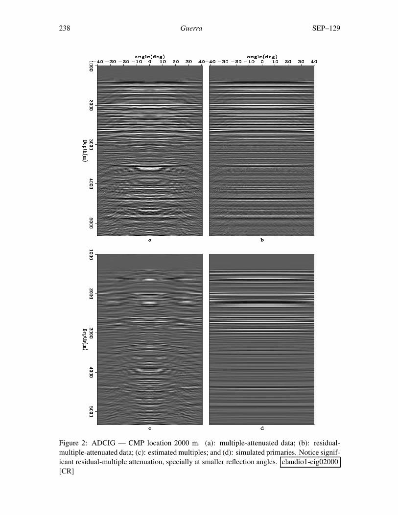
Another issue in methods that rely on the moveout difference between primaries and mul-tiples is the persistence of multiples in the near angles (or offsets) due to insufficient moveoutdifference between them and the primaries. In sub-salt regions, this problem is especiallyprominent in ADCIGs because of the poor illumination of larger angles. To guarantee thatresidual multiples in the near-angle range do not interfere with the computation of the sim-ulated primaries, I applied an internal mute, roughly below depth=3000 m between angles−10◦ and 10◦. At the CMP location 12000 m; what may seem to be primaries in the nearangle are actually residual multiples, as can be clearly seen in the zero-angle section (Figure


Figure 2: ADCIG — CMP location 2000 m. (a): multiple-attenuated data; (b): residual-multiple-attenuated data; (c): estimated multiples; and (d): simulated primaries. Notice signif-icant residual-multiple attenuation, specially at smaller reflection angles. claudio1-cig02000[CR]


Figure 3: ADCIG — CMP location 12000 m. (a): multiple-attenuated data; (b): residual-multiple-attenuated data; (c): estimated multiples; and (d): simulated primaries. Notice signif-icant residual-multiple attenuation, specially at smaller reflection angles. claudio1-cig12000[CR]


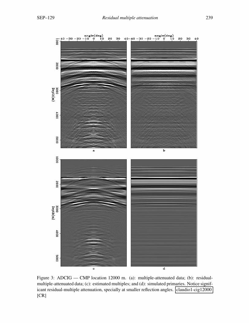
Figure 4: ADCIG — CMP location 20000 m. (a): multiple-attenuated data; (b): residual-multiple-attenuated data; (c): estimated multiples; and (d): simulated primaries. Notice, in theestimated residual-multiples panel, the apex of diffracted multiples (around depth = 3700 m)located at reflection angles = ±20◦. claudio1-cig20000 [CR]


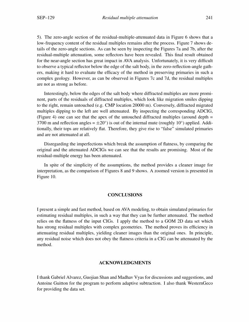
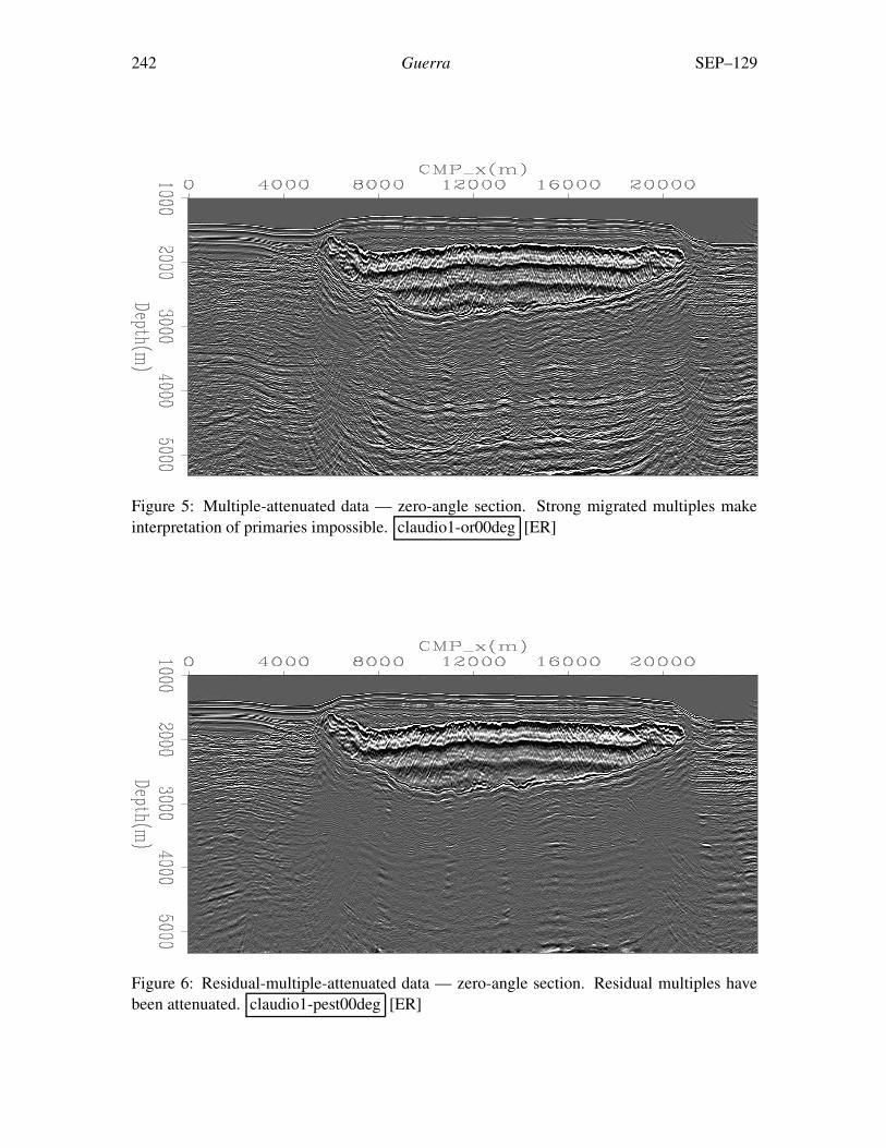
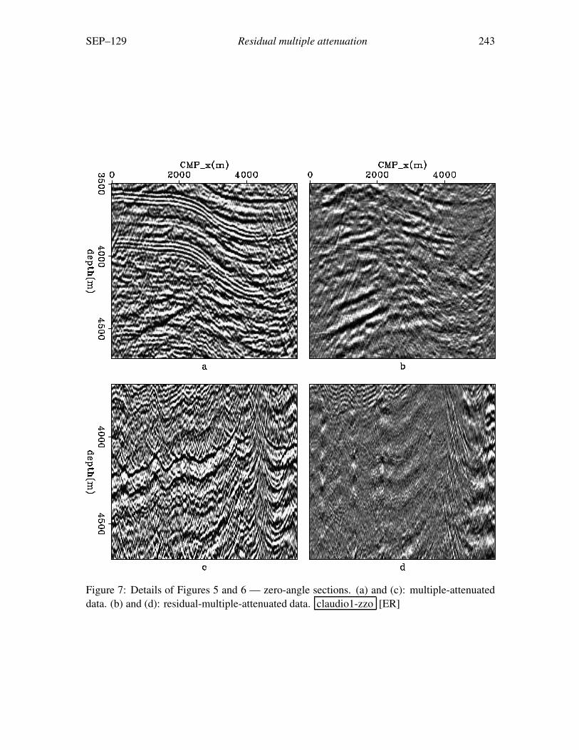
5). The zero-angle section of the residual-multiple-attenuated data in Figure 6 shows that alow-frequency content of the residual multiples remains after the process. Figure 7 shows de-tails of the zero-angle sections. As can be seen by inspecting the Figures 7a and 7b, after theresidual-multiple attenuation, some reflectors have been revealed. This final result obtainedfor the near-angle section has great impact in AVA analysis. Unfortunately, it is very difficultto observe a typical reflector below the edge of the salt body, in the zero-reflection-angle gath-ers, making it hard to evaluate the efficacy of the method in preserving primaries in such acomplex geology. However, as can be observed in Figures 7c and 7d, the residual multiplesare not as strong as before.

Interestingly, below the edges of the salt body where diffracted multiples are more promi-nent, parts of the residuals of diffracted multiples, which look like migration smiles dippingto the right, remain untouched (e.g. CMP location 20000 m). Conversely, diffracted migratedmultiples dipping to the left are well attenuated. By inspecting the corresponding ADCIG,(Figure 4) one can see that the apex of the untouched diffracted multiples (around depth =3700 m and reflection angles = ±20◦) is out of the internal mute (roughly 10◦) applied. Addi-tionally, their tops are relatively flat. Therefore, they give rise to “false” simulated primariesand are not attenuated at all.

Disregarding the imperfections which break the assumption of flatness, by comparing theoriginal and the attenuated ADCIGs we can see that the results are promising. Most of theresidual-multiple energy has been attenuated.

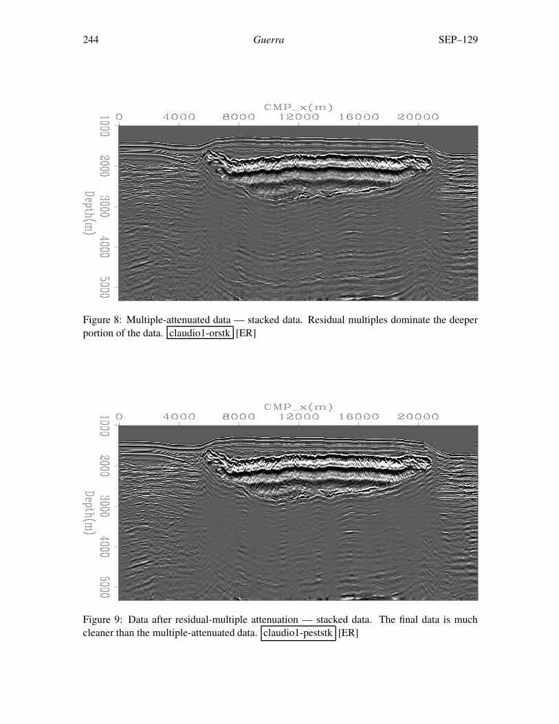
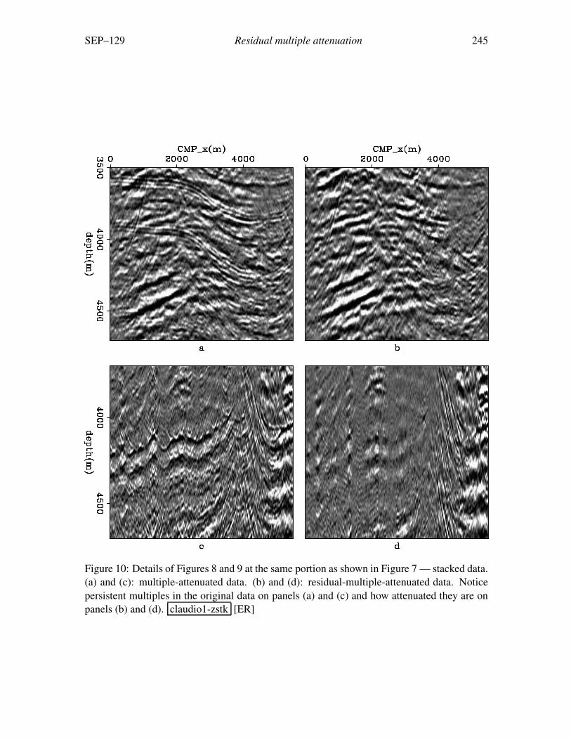
In spite of the simplicity of the assumptions, the method provides a cleaner image forinterpretation, as the comparison of Figures 8 and 9 shows. A zoomed version is presented inFigure 10.

CONCLUSIONS

I present a simple and fast method, based on AVA modeling, to obtain simulated primaries forestimating residual multiples, in such a way that they can be further attenuated. The methodrelies on the flatness of the input CIGs. I apply the method to a GOM 2D data set whichhas strong residual multiples with complex geometries. The method proves its efficiency inattenuating residual multiples, yielding cleaner images than the original ones. In principle,any residual noise which does not obey the flatness criteria in a CIG can be attenuated by themethod.

ACKNOWLEDGMENTS

I thank Gabriel Alvarez, Guojian Shan and Madhav Vyas for discussions and suggestions, andAntoine Guitton for the program to perform adaptive subtraction. I also thank WesternGecofor providing the data set.


Figure 5: Multiple-attenuated data — zero-angle section. Strong migrated multiples makeinterpretation of primaries impossible. claudio1-or00deg [ER]

Figure 6: Residual-multiple-attenuated data — zero-angle section. Residual multiples havebeen attenuated. claudio1-pest00deg [ER]


Figure 7: Details of Figures 5 and 6 — zero-angle sections. (a) and (c): multiple-attenuateddata. (b) and (d): residual-multiple-attenuated data. claudio1-zzo [ER]


Figure 8: Multiple-attenuated data — stacked data. Residual multiples dominate the deeperportion of the data. claudio1-orstk [ER]

Figure 9: Data after residual-multiple attenuation — stacked data. The final data is muchcleaner than the multiple-attenuated data. claudio1-peststk [ER]


Figure 10: Details of Figures 8 and 9 at the same portion as shown in Figure 7 — stacked data.(a) and (c): multiple-attenuated data. (b) and (d): residual-multiple-attenuated data. Noticepersistent multiples in the original data on panels (a) and (c) and how attenuated they are onpanels (b) and (d). claudio1-zstk [ER]


REFERENCES

Aki, K. and P. Richards, 1980, Quantitative seismology: W.H.Freeman and Co.

Alvarez, G., B. Biondi, and A. Guitton, 2004, Attenuation of diffracted multiples with anapex-shifted tangent-squared radon transform in image space: SEP–115, 139–152.

Choo, J., J. Downton, and J. Dewar, 2004, Lift: A new and practical approach to noise andmultiple attenuation: First Break, 22, no. 5, 39–44.

Claerbout, J. and S. Fomel, 2001, Image estimation by example: Geophysical soundings imagereconstruction: http://sepwww.stanford.edu/sep/prof/gee2.06.pdf.

Guitton, A., M. Brown, J. Rickett, and R. Clapp, 2001, A pattern-based technique for ground-roll and multiple attenuation: SEP–108, 249–274.

Hampson, D., 1987, The discrete Radon transform: A new tool for image enhancement andnoise suppression: Soc. of Expl. Geophys., 57th Ann. Internat. Mtg, Soc. Expl. Geophys.,Expanded Abstracts, Session:BP3.CSEG.

Verschuur, D. J., A. J. Berkhout, and C. P. A. Wapenaar, 1992, Adaptive surface-related mul-tiple elimination: Geophysics, 57, no. 9, 1166–1177.

Weglein, A. B., 1999, Multiple attenuation: An overview of recent advances and the roadahead: The Leading Edge, 18, no. 1, 40–44.

262 SEP–129

Documents

Stanford Exploration Project, Report 129, May 6, 2007 ...sep Exploration Project, Report 129, May 6, 2007, ... phase of the simulated primaries to the amplitude and ... where M is