Cosmological inference using only gravitational wave observations of binary neutronstars

Walter Del Pozzo∗

School of Physics and Astronomy, University of Birmingham,Edgbaston, Birmingham B15 2TT, United Kingdom and

Dipartimento di Fisica “Enrico Fermi”, Universita di Pisa, Pisa I-56127, Italy

Tjonnie G.F. LiLIGO - California Institute of Technology, Pasadena, CA 91125, USA and

Department of Physics, The Chinese University of Hong Kong, Shatin, N.T., Hong Kong

Chris MessengerSUPA, School of Physics and Astronomy, University of Glasgow, Glasgow G12 8QQ, United Kingdom

(Dated: January 12, 2017)

Gravitational waves emitted during the coalescence of binary neutron star systems are self-calibrating signals. As such, they can provide a direct measurement of the luminosity distanceto a source without the need for a cross-calibrated cosmic distance-scale ladder. In general, how-ever, the corresponding redshift measurement needs to be obtained via electromagnetic observationssince it is totally degenerate with the total mass of the system. Nevertheless, Fisher matrix studieshave shown that, if information about the equation of state of the neutron stars is available, it is pos-sible to extract redshift information from the gravitational wave signal alone. Therefore, measuringthe cosmological parameters in pure gravitational-wave fashion is possible. Furthermore, the hugenumber of sources potentially observable by the Einstein Telescope has led to speculations that thegravitational wave measurement is potentially competitive with traditional methods. The EinsteinTelescope is a conceptual study for a third generation gravitational wave detector which is designedto yield 103 − 107 detections of binary neutron star systems per year. This study presents the firstBayesian investigation of the accuracy with which the cosmological parameters can be measuredusing information coming only from the gravitational wave observations of binary neutron star sys-tems by Einstein Telescope. We find, by direct simulation of 103 detections of binary neutron stars,that, within our simplifying assumptions, H0,Ωm,ΩΛ, w0 and w1 can be measured at the 95% levelwith an accuracy of ∼ 8%, 65%, 39%, 80% and 90%, respectively. We also find, by extrapolation,that a measurement accuracy comparable with current measurements by Planck is possible if thenumber of gravitational wave events observed is O(106−7).We conclude that, while not competitivewith electro-magnetic missions in terms of significant digits, gravitational wave alone are capable ofproviding a complementary determination of the dynamics of the Universe.

I. INTRODUCTION

The family of second generation interferometers Ad-vanced LIGO [1] began its operations in the last quarterof 2015 [2]. Advanced Virgo [3] is scheduled to join theLIGO network in 2017, with KAGRA [4] and LIGOIndia [5] to follow afterwards. The detection of grav-itational waves from the coalescence of merging blackholes [6–8] led already to important scientific measure-ments as tests of general relativity [8, 9] and astrophysics[8, 10, 11]. Given the expected number of yearly detec-tions [8, 12, 13], the expectations on the scientific deliv-erables are high: tests of the strong field dynamics ofGeneral Relativity [8, 9, 14–16]; a “cosmic distance scaleladder”-free determination of the Hubble constant [17–19]; a determination of the neutron star equation equa-tion of state [20–23].

Detectors beyond the second generation are alreadybeing envisaged. For instance, the Einstein gravitational

∗ walter.delpozzo@unipi.it

wave Telescope (ET) [24] is a proposed underground de-tector consisting of three 10 km arm-long Michelson in-terferometers in a triangular topology with opening an-gles of 60 degrees [25]. The strain sensitivity is estimatedas factor 10 better than second generation detectors,down to frequencies of 1− 3 Hz depending on the actualconfiguration of the instrument [26]. The high sensitivitypromises the detection of a very large number of gravi-tational waves (GW) signals with large signal-to-noiseratios (SNR), thus allowing for unprecedented popula-tion studies as well as extremely accurate measurementsof the physical parameters of coalescing binary systems[24].

A. Cosmological inference with gravitational waves

When estimating the parameters of GW sources, andin particular the coalescences of binary neutron stars andblack holes, the luminosity distance can be observed di-rectly [27, 28]. This makes GW an ideal laboratory toplace samples in the Hubble diagram in a manner that is

arX

iv:1

506.

0659

0v2

[gr

-qc]

11

Jan

2017

2

free from the potential systematics affecting electromag-netic (EM) methods. Unfortunately, in the vast majorityof the cases, the redshift cannot be measured from GWalone and this piece of information needs to be extractedby means other than GW.

In the recent years, various proposals have been putforward to overcome this difficulty. For instance, onecan assume that the coalescences of compact binaries arethe progenitors of short gamma ray bursts (sGRB) [29].In this case, coincident observations of a GW event andthe correspondent sGRB would allow the measurement ofthe luminosity distance from GW and the redshift fromspectroscopy of the host galaxy[17, 30–32]1. For secondgeneration interferometers, this method indicates a rela-tive accuracy on the measurement of the Hubble constantH0 of few percent in the case where 10-15 such events aredetected. However, whether the coalescences of compactbinaries are the progenitors of sGRBs is still a matterof debate. Also, the fraction of GW events also observ-able as sGRBs might be as low as 10−3[35] due to sGRBbeaming effects.

An alternative approach, following broadly the argu-ment first given in Ref. [27], would be to statisticallyidentify the possible host galaxies of a GW event to ob-tain a distribution of possible redshifts associated witheach GW detection. This method should yield ∼ 5%percent accuracy on H0 using 20-50 events [18] observedby Advanced LIGO/Virgo. A similar methodology hasalso been applied to space-based detectors [36, 37].

A few methods aim at extracting the redshift usingGW observations alone. For example, one can use theknowledge of the (rest frame) mass function of NS andthe measured (redshifted) mass to infer the redshift ofthe source [19, 38]. In this framework, second generationinterferometers should infer the Hubble constant H0 with∼ 10% accuracy using about 100 events [19].

The results of advanced interferometers can be greatlyimproved by third generation instruments such as ET. Infact, ET can probe regions of the Universe where the ef-fects of the dark energy will be substantial, thus allowingan independent sampling of the cosmic history.

The potentialities of ET have already been investigatedby various groups [30, 31, 39], concluding that, when onlya limited set of cosmological parameters is considered, theaccuracy of the inference is comparable to that of currentEM measurements.

B. Outline

In this paper, we will expand on the approach pro-posed by Messenger and Read [40] in which if one of the

1 Kilonovae are also expected EM counterparts to BNS coales-cences [33]. However their utility as cosmological probes is yetunclear due to their intrinsically faint luminosities [e.g. 34] whichlimits the distance at which they can be confidently detected.

two components is a NS, information about the equa-tion of state (EOS) allows a direct measurement of therest-frame masses and thus of the source redshift [40].Using Fisher matrix formalism, the authors estimate theaccuracy with which z can be measured to be ∼ 8−40%,depending on the EOS and on the distance to the source.Recently, a similar investigation was carried out in [41]using a more realistic Monte Carlo data analysis method.The authors concluded that the average uncertainty iscloser to 40% for a hard EOS and essentially indepen-dent of redshift.

Nevertheless, given the large number of sources thatcan be observed by ET and the possibility of combininginformation across them, even the large uncertainty re-ported in Ref. [41] could be sufficient to obtain interestingindications on the accuracy with which ET will measurethe cosmological parameters. In this paper, we explorethis idea in a simplified scenario and conclude that ETcan indeed set bounds that are comparable to currentEM measurement. We are interested in the cosmologicalinformation that can be inferred exclusively from the ob-servation of gravitational waves. We will thus not discussthe potential of coincident GW-EM detections which arepresented elsewhere [31, 39]. We note here that, becauseof the co-location of the three ET interferometers andbecause of its topology, its expected sky resolution is ex-tremely poor. Consequently, the probability of a success-ful EM-GW association is a priori very small. Note thatat the time of ET, second generation detectors are ex-pected to be operational with improved sensitivities [42].For a substantial fraction of the loudest GW events, thesky localisation from a network made of ET and advanceddetectors will be vastly improved compared to ET alone.In this case, some of the aforementioned EM+GW meth-ods might become feasible and used to yield constraintson the cosmological parameters.

The rest of the paper is organised as follows. In foot-note 1 we cast the problem in a Bayesian framework, andidentify the necessary components to arrive at the cosmo-logical inference. In Eq. (10) we describe the proceduresof simulating GW events and the detector noise, and theimplementation of the analysis. In Fig. 3 we present theresults of our simulations and finally in table III we sum-marise and discuss our results. The mathematical solu-tion to the problem of the inference of the cosmologicalparameters in the presence of a detection threshold isgiven for completeness in Appendix A.

II. METHOD

In this section we present a Bayesian solution to theproblem of computing posterior probability density func-tions for a set of cosmological parameters from GW data.We broadly follow the presentation in [18]. Note that thetreatment is not specific to the case of ET.

3

A. Inference of the cosmological parameters in theabsence of a detection threshold

Consider a catalogue of GW events E ≡ ε1, . . . , εN.Each event is defined as a stretch of data di(t) given bythe sum of noise ni(t) and a gravitational wave signal

hi( ~Θi; t), i.e.

εi : di(t) = ni(t) + hi(~Θi; t) , (1)

where ~Θi indicates the set of all parameters of the signali.

The noise is taken to be a stationary Gaussian processwith a zero mean and covariance defined by its one-sidedspectral density Sn(f) such that

p(ni|I) ∝ exp

−1

2

∫ ∞0

df 4|ni(f)|2

Sn(f)

,

∝ exp

−1

2(n | n)

(2)

where I represents all the relevant information for the in-ference problem, a tilde represents the Fourier transform,and where we have introduced a scalar product betweentwo real functions A(t) and B(t) as

(A| B) = 4<∫ ∞

0

dfA∗(f)B(f)

Sn(f). (3)

The likelihood of observing the event εi is then given by

p(εi|~Θi,S, I) ∝ exp

−1

2(di − hi | di − hi)

(4)

where S is the signal model that relates the signal param-

eters ~Θi to a gravitational wave signal h. Moreover, thesignal-to-noise ratio (SNR) ρ can be succinctly writtenas

ρ =√

(h | h) . (5)

The posterior distribution for any parameter in our signalmodel S is related to the likelihood in Eq. (4) through theapplication of Bayes’ theorem

p(~Θi|εi,S, I) ∝ p(~Θi|S, I)p(εi|~Θi,S, I) (6)

where p(~Θi|S, I) is the prior probability distribution for

the parameters ~Θi. When multiple independent detec-tors are included in the analysis, the likelihood (Eq. (4))generalises to

p(εi|~Θi,S, I) =∏k

p(ε(k)i |~Θi,S, I) . (7)

For this work, we are only interested in the pos-

terior probability for a subset of parameters ~Ω ≡

H0,Ωm,ΩΛ, . . .. Therefore, we marginalise over the

remaining subset of parameters ~θi, i.e.

p(~Ω|εi,S, I) =

∫d~θi p(~Θi|εi,S, I)

=

∫d~θi p(~θi, ~Ω|S, I)p(εi|~θi, ~Ω,S, I)

= p(~Ω|S, I)∫

d~θi p(~θi|~Ω,S, I)p(εi|~θi, ~Ω,S, I)

= p(~Ω|S, I)L(εi, ~Ω) , (8)

Where we have introduced the so-called “quasi-likelihood” [43]

L(εi, ~Ω) ≡∫

d~θi p(~θi|~Ω,S, I)p(εi|~θi, ~Ω,S, I). (9)

Finally, the posterior for ~Ω given an ensemble of eventsE can be shown to be

p(~Ω|E ,S, I) = p(~Ω|S, I)∏i

L(εi, ~Ω). (10)

Therefore, in order to obtain the posterior for ~Ω, we needto perform a multi-dimensional integral in Eq. (9) foreach of the GW events. The description of this procedureand the generation of data follow in Eq. (10).

III. ANALYSIS

In this section we describe the simulation that was per-formed. Firstly, we outline the generation of the data,consisting of the GW signal model, the astrophysical andcosmological assumptions regarding the source popula-tion, and the simulation of the detector noise. Secondly,we show the data analysis implementation with whichthe simulated data was analysed. In particular, we de-scribe the construction of the quasi-likelihood, and it sub-sequent use to arrive at our cosmological inference. TheGW signals, and the detector noise have been generatedusing the LIGO Analysis library (LAL) [44].

A. Astrophysical and cosmological assumptions

The NS masses are distributed according to a Gaussiandistribution with a mean of 1.35M and a standard devi-ation of 0.15M [45] which is assumed constant through-out the cosmic history. For the NS equation of statewe consider three cases; a hard EOS, a medium and asoft EOS. They are labelled as MS1 [46], H4 [47] andSQM3 [48]. We investigate these three cases since in [40]it was shown that the accuracy with which the redshiftcan be measured depends on the magnitude of the phys-ical effects related to the details of the EOS. One canthink of these three cases as an optimistic, a realisticand a pessimistic one, respectively.

4

The events are distributed uniformly in the cosine ofthe inclination, polarisation and time of arrivals. Theevents are also uniformly distributed in comoving vol-ume. Their redshifts are sampled from the probabilitydensity given by [49]

p(z|~Ω) =dR(z)

dz

1

R(zmax)(11)

where R(z) is the cosmic coalescence rate. It is worth

nothing that p(z|~Ω) is an explicit function of ~Ω. Thedifferential cosmic coalescence rate is equal to

dR(z)

dz=

dV

dz

r0e(z)

1 + z(12)

where r0 is the local rate, e(z) is the cosmic star forma-tion rate and V is the comoving volume. In a Friedmann-Robertson-Walker-Lemaitre (FRWL) universe, the rateof change of V with z is given by

dV

dz= 4π

D2L(z)

(1 + z)2H(z), (13)

where we have introduced the Hubble parameter

H(z) = H0

√Ωm(1 + z)3 + Ωk(1 + z)2 + ΩΛE(z, w(z))

(14)

and the luminosity distance [50]

DL(z) =

(1+z)√

Ωksinh[

√Ωk∫ z

0dz′

H(z′) ] for Ωk > 0

(1 + z)∫ z

0dz′

H(z′) for Ωk = 0(1+z)√|Ωk|

sin[√|Ωk|

∫ z0

dz′

H(z′) ] for Ωk < 0

(15)

H0 is the Hubble constant, Ωm is the matter fractionaldensity, ΩΛ is the fractional energy density of dark en-ergy, Ωk = 1− Ωm − ΩΛ is the curvature. Finally

E(z, w(z)) = (1 + z)3(1+w0+w1)e−3w1z/(1+z) (16)

is a convenient parametrisation to capture the effects of

the redshift evolution of dark energy [51]. For ~Ω we chosefiducial values of

(h,Ωm,ΩΛ,Ωk, w0, w1)fid = (0.7, 0.3, 0.7, 0,−1, 0), (17)

where h = H0/100km·Mpc−1·s−1. Even though ET hori-zon distance is ' 37 Gpc (z ' 4.15 for our fiducial cos-mology), we limit our analysis to zmax = 2 as this corre-sponds approximately the sky averaged horizon distanceof 13 Gpc for BNS systems [52]. For simplicity, we de-cided to assume a star formation rate e(z) that does notchange with redshift and is therefore irrelevant for ourproblem.

We simulated 1,000 binary NS events as observed byET. The parameters θi of each individual source havebeen generated according to the assumptions described in

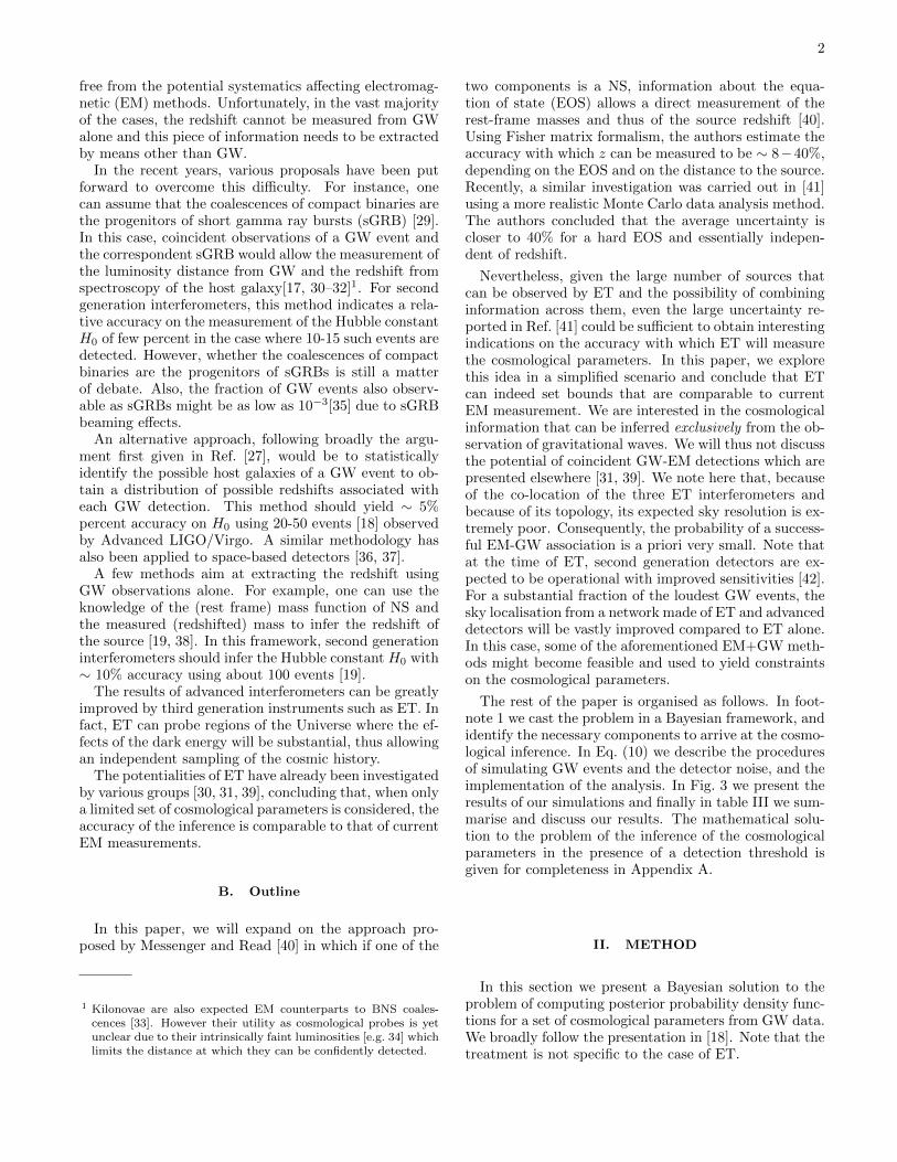
5 10 20 50SNR

0.00

0.02

0.04

0.06

0.08

0.10

0.12

0.14

0.16

relative

frequency

FIG. 1. Network SNR distribution of the 1,000 BNS eventsgenerated sampling Eqs. (11) and (13) for a our fiducial cos-mology Eq. (17).

Eq. (10). The corresponding waveform h(f, ~Θi) was thenadded to Gaussian noise which is coloured according tothe amplitude spectral density shown in Fig. 2. In Fig. 1we show the network SNR distribution in the ET detectorcomputed using Eq. (5).

Differently from most existing literature, we do not fil-ter our sources with any SNR threshold. If we were to doso, we would be introducing a selection bias [53]. Notethat, due to the potentially large number of sources ob-served by ET and their distribution in co-moving volume,the vast majority of them will in practice not be detectedin a search which uses the SNR as decision statistics. It isknown that ignoring these unregistered sources leads to asignificant bias in the estimation of “global” parameters,see [53].

The main reason for the emergence of biases is inti-mately linked to the functional form for the prior onz Eq. (11). Since Eq. (11) quantifies the prior expec-tation regarding the distribution of sources in the co-

moving volume, it is an explicit function of ~Ω. The quasi-likelihoods for the majority of our simulated events are

almost uniform in ~Ω, see Section III C 2, therefore ourinference is greatly influenced by the prior distribution:if one were to analyse sources that are louder than somethreshold SNR the overall population of events wouldappear on average closer than the actual population. Atthe same time, the observed distribution of z would fol-

low the actual cosmological distribution. Since p(z|~Ω)

Eq. (11) relates DL and z via ~Ω, this leads for estimatesof Ωm → 1 and h→ 0. Similarly, if one were to consideronly events that are quieter than a given SNR thresh-old, Ωm → 0 and h → 1, thus ΩΛ → 1. In AppendixA, we give a mathematical solution to the problem of

inferring ~Ω that accounts for sets of unobserved events.However, the solution in A is not computationally treat-able with current techniques and for a large number ofevents, therefore we opted for an SNR selection thresholdof 0 and analysed all simulated events. Furthermore, our

5

choice relies on the capacity of distinguishing betweenlow SNR GW signals and low SNR background eventsdue to noise in the detector. A discussion of this prob-lem can be found in [53]. The triangular configuration ofET provides an additional tool to study the distributionof signal and noise low SNR events. Thanks to its topol-ogy, ET admits the construction of a null stream which isdevoid of any GW signal as the sum of the outputs of theindividual Michelson detectors [25]. Being a pure noiseprocess, the analysis of the null stream can be used tounderstand the SNR distribution of noise events whichcan then be used to infer the SNR distribution of quietsources.

B. The signal model

In the previous paragraph we introduced the signalmodel S without specifying its properties. In this section,we lay out the assumptions that go in the constructionof S.

In modelling the GW from a binary system, we limitour analysis to the inspiral phase of the coalescence pro-cess. We model the inspiral using an analytical frequencydomain 3.5 post-Newtonian waveform in which we ig-nore amplitude corrections and the effects of spins. Thisis not a big limitation as NS are expected to be slowrotators[54]. In particular, we use the so-called TaylorF2approximant [55], which can be written as

h(~Θ; f) = A(~Θ)f−7/6eiΦ(~Θ;f) , (18)

where the waveform is written in terms of the amplitude

A(~Θ) and the phase Φ(~Θ; f).

The amplitude of the waveform A(~Θ) is given by

A(~Θ) ∝ M5/6

DLQ(ι, ψ, α, δ) (19)

where we have introduced the chirp mass M =

m3/51 m

3/52 /(m1 + m2)1/5, DL is the luminosity distance

defined in Eq. (15), (α, δ) signify the sky position of thesource, and (ι, ψ) give the orientation of the binary withrespect to the line of sight [55].

The wave phase can be written in the form

Φ(~Θ; f) = 2πftc − φc −π

4

+

7∑n=0

[ψn + ψ(l)

n ln f]f (n−5)/3, (20)

where the ψn are the so-called post-Newtonian coeffi-cients (see e.g. [56]), which are functions of the com-ponent masses m1 and m2, and (tc, φc) are the time andphase of coalescence. Note that all masses are definedin the observer frame, and the rest frame mass mrest isrelated to the observed mass through

m = mrest(1 + z) , (21)

where z is the redshift of the GW source.The description of the phase in Eq. (20) assumes that

the object is a point particle, and thus cannot be tidallydeformed. However, since we consider all of our eventsare binary NS coalescences, we modify the gravitationalwave phase in Eq. (20) by including the finite-size contri-butions to the phase. These in turn depend on the tidaldeformability λ(mrest) [21] of the star which is a func-tion of its equation of state and its rest frame mass. Thefinite-size contributions to the GW phase, as a functionof observed masses, is given by

Φtidal(~Θ; f) =

2∑a=1

3λa(1 + z)5

128ηM5

[− 24

χa

(1 +

11η

χa

)(πMf)5 − 5

28χa

(3179− 919χa − 2286χ2

a + 260χ3a

)(πMf)7

],

(22)

where the sum is over the components of the binary, χa =ma/M , λa = λ(ma) where ma are the component masses,M is the total mass, and η = m1m2/M

2.

Knowledge of the EOS and using information encodedin the GW tidal phase contribution allows to measurethe redshift of the source [40]. While the EOS is notknown yet, various studies have shown that it could bepossible to infer it from observations of BNS with secondgeneration detectors [20–23, 57, 58]. In what follows, wewill assume that the nature of the NS interior is known.

C. Data analysis

For our analysis, we assumed a noise curve for ET cor-responding to the “B” configuration [59], correspondingto the projected sensitivity achievable with the currenttechnologies Fig. 2. Given the anticipated rates of com-pact binary coalescences [13], the detection rates of bi-nary NS systems in ET are expected to lie in the range103 − 107 yr−1[24].

The parameters ~θ of our signal model are the compo-nent masses m1 and m2, inclination ι, polarisation ψ,

6

101 102 103

Hz

10-2

10-1

100

1023√ S

n(f

)H

z−1/

2

FIG. 2. Amplitude spectral density for ET in the “B” config-uration.

right ascension α and declination δ, the time of coales-cence tc, the phase of coalescence φc, luminosity distanceDL and the redshift z. In our analysis we ignored thepresence of spins, as it is believed to be small in binaryNS systems[54]. We analysed our ensemble of sourcesassuming that the EOS of the NS is known, thus ac-counting to a total of three analysis runs (one for each ofour predefined hard, medium and soft EOSs). To obtainthe posterior probability distribution on the cosmologi-

cal parameters ~Ω we proceeded in three steps. Firstly,we analysed each source to compute a quasi-likelihood asa function of the redshift z and the luminosity distanceDL. Secondly, these quasi-likelihoods are then convertedinto quasi-likelihoods as a function of the cosmological

parameters ~Ω as shown in Eq. (9). Finally, the poste-rior probability function for the cosmological parametersgiven an ensemble of events are computed from Eq. (10).

1. Obtaining the quasi-likelihood

For each event εi, we compute the quantity

L(εi, DL, z, ~Ω) ≡∫

d~λ p(~λ|~Ω,S, I)p(εi|~λ, ~Ω,S, I) (23)

that is a partially marginalised quasi-likelihood, wherethe marginalisation is done on all parameters that are

not relevant to the inference of ~Ω. These are ~λ ≡(m1,m2, ψ, ι, φc, tc, α, δ). The further marginalisationover z and DL will be described later on. For the time be-ing, let us describe the details of the analysis for the com-putation of Eq. (23). The above integral was computedusing a Nested Sampling algorithm [60] implemented sim-ilarly to what described in [61]. For each of the threeanalysis runs, we chose the same prior probability dis-tributions for all parameters, with the exception of the

component masses. For the common parameters we useduniform probability distributions on the 2-sphere for skyposition (α, δ) and orientation (ψ, ι) and uniform in thetime of coalescence tc with a width of 0.1 seconds aroundthe actual coalescence time. For the first marginalisa-tion, we choose uniform sampling distributions for bothDL and z in the intervals [1, 105] Mpc and [0,2], respec-tively.

For the component masses, the priors were differentacross the different runs; each EOS in fact predicts notonly the functional form of the tidal deformability λ(m)that enters in the phase of the GW waveform, but alsothe maximum permitted mass of the NS itself. Therefore,for the three EOSs under consideration we used maxi-mum expected rest frame mass Mmax of 2.8, 2.0, 2.0Mfor MS1, H4 and SQM3 respectively. The prior prob-ability distribution for the component masses was thenchosen to be uniform between 1M and Mmax.

2. Cosmological inference

The marginalisation over the redshift and luminositydistance was then performed as follows: once a cosmolog-ical model is introduced, z and DL are not independentparameters anymore, but they are related unequivocallyby Eq. (15), thus – after some algebra which can be foundin [18] – we are left with the following integral to compute

L(εi, ~Ω) =

∫ zmax

0

dz p(z|~Ω, SI)L(εi, DL(z), z, ~Ω) , (24)

where p(z|~Ω, SI) is given in Eq. (11) and we chose, con-sistently with the sources generation, zmax = 2.

One of the problems we needed to overcome in orderto perform the integral in Eq. (24) was how to represent

L(εi, DL(z), z, ~Ω) in a tractable way. In fact, one of theoutputs of the Nested Sampling algorithm is a set of sam-ples drawn from the integrand in Eq. (23) which is dif-ficult to manipulate – in particular difficult to integrate– without making any assumptions about the underlyingprobability distribution.

A possible treatment of the problem would be to usethe samples from Eq. (23) and approximate it using a nor-malised histogram. This procedure was successfully usedin other unrelated studies [14], however, for our purposesit is not accurate enough. In fact, an histogram represen-tation is dependent on a parameter, the bin size (or equiv-alently the number of bins once the range is specified),which cannot be inferred from the data but has to bechosen arbitrarily. The majority of the quasi-likelihoodsin Eq. (24) tend to be very uniform over the cosmologicalparameter space for individual sources and, as noted inSection III A, the inference is strongly dominated by theprior on z. Most sources are close or below the detectionthreshold of the detector, thus a single source, in general,yields very little information about the underlying cos-mology, therefore any small fluctuation in the histogram

7

approximation due to the random variation of the num-ber of samples in any specific bin would be amplified andwould eventually lead to a biased estimate of the poste-

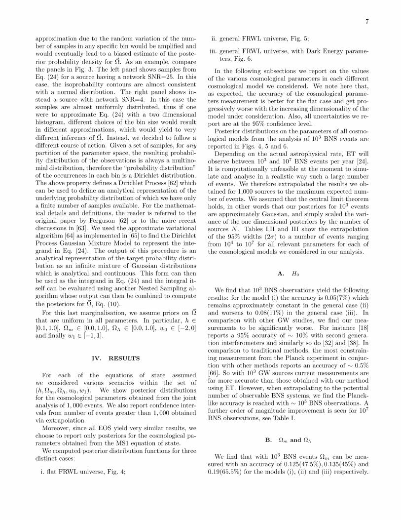
rior probability density for ~Ω. As an example, comparethe panels in Fig. 3. The left panel shows samples fromEq. (24) for a source having a network SNR=25. In thiscase, the isoprobability contours are almost consistentwith a normal distribution. The right panel shows in-stead a source with network SNR=4. In this case thesamples are almost uniformly distributed, thus if onewere to approximate Eq. (24) with a two dimensionalhistogram, different choices of the bin size would resultin different approximations, which would yield to very

different inference of ~Ω. Instead, we decided to follow adifferent course of action. Given a set of samples, for anypartition of the parameter space, the resulting probabil-ity distribution of the observations is always a multino-mial distribution, therefore the “probability distribution”of the occurrences in each bin is a Dirichlet distribution.The above property defines a Dirichlet Process [62] whichcan be used to define an analytical representation of theunderlying probability distribution of which we have onlya finite number of samples available. For the mathemat-ical details and definitions, the reader is referred to theoriginal paper by Ferguson [62] or to the more recentdiscussions in [63]. We used the approximate variationalalgorithm [64] as implemented in [65] to find the DirichletProcess Gaussian Mixture Model to represent the inte-grand in Eq. (24). The output of this procedure is ananalytical representation of the target probability distri-bution as an infinite mixture of Gaussian distributionswhich is analytical and continuous. This form can thenbe used as the integrand in Eq. (24) and the integral it-self can be evaluated using another Nested Sampling al-gorithm whose output can then be combined to compute

the posteriors for ~Ω, Eq. (10).

For this last marginalisation, we assume priors on ~Ωthat are uniform in all parameters. In particular, h ∈[0.1, 1.0], Ωm ∈ [0.0, 1.0], ΩΛ ∈ [0.0, 1.0], w0 ∈ [−2, 0]and finally w1 ∈ [−1, 1].

IV. RESULTS

For each of the equations of state assumedwe considered various scenarios within the set of(h,Ωm,ΩΛ, w0, w1). We show posterior distributionsfor the cosmological parameters obtained from the jointanalysis of 1, 000 events. We also report confidence inter-vals from number of events greater than 1, 000 obtainedvia extrapolation.

Moreover, since all EOS yield very similar results, wechoose to report only posteriors for the cosmological pa-rameters obtained from the MS1 equation of state.

We computed posterior distribution functions for threedistinct cases:

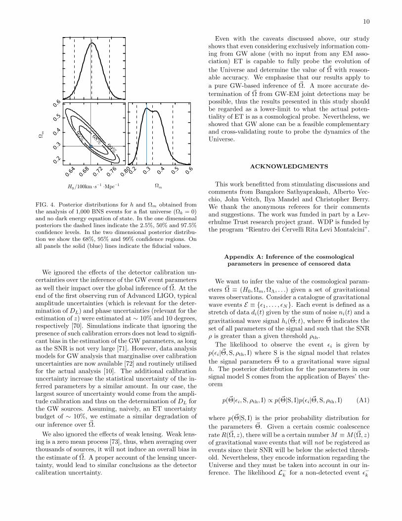
i. flat FRWL universe, Fig. 4;

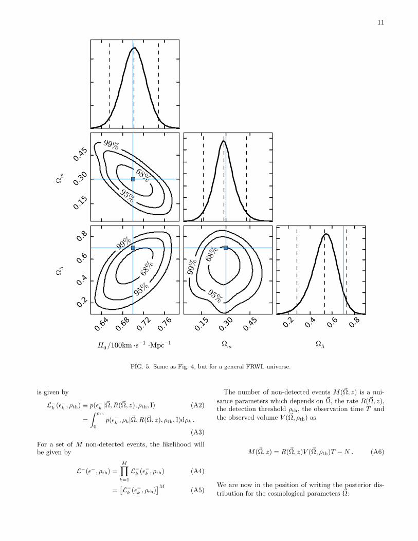
ii. general FRWL universe, Fig. 5;

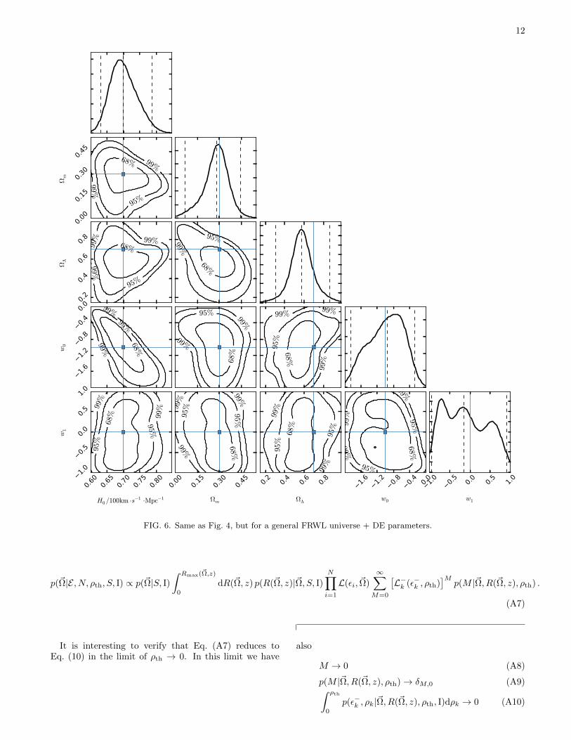
iii. general FRWL universe, with Dark Energy parame-ters, Fig. 6.

In the following subsections we report on the valuesof the various cosmological parameters in each differentcosmological model we considered. We note here that,as expected, the accuracy of the cosmological parame-ters measurement is better for the flat case and get pro-gressively worse with the increasing dimensionality of themodel under consideration. Also, all uncertainties we re-port are at the 95% confidence level.

Posterior distributions on the parameters of all cosmo-logical models from the analysis of 103 BNS events arereported in Figs. 4, 5 and 6.

Depending on the actual astrophysical rate, ET willobserve between 103 and 107 BNS events per year [24].It is computationally unfeasible at the moment to simu-late and analyse in a realistic way such a large numberof events. We therefore extrapolated the results we ob-tained for 1,000 sources to the maximum expected num-ber of events. We assumed that the central limit theoremholds, in other words that our posteriors for 103 eventsare approximately Gaussian, and simply scaled the vari-ance of the one dimensional posteriors by the number ofsources N . Tables I,II and III show the extrapolationof the 95% widths (2σ) to a number of events rangingfrom 104 to 107 for all relevant parameters for each ofthe cosmological models we considered in our analysis.

A. H0

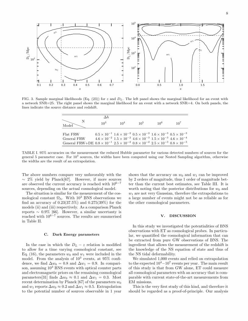
We find that 103 BNS observations yield the followingresults: for the model (i) the accuracy is 0.05(7%) whichremains approximately constant in the general case (ii)and worsens to 0.08(11%) in the general case (iii). Incomparison with other GW studies, we find our mea-surements to be significantly worse. For instance [18]reports a 95% accuracy of ∼ 10% with second genera-tion interferometers and similarly so do [32] and [38]. Incomparison to traditional methods, the most constrain-ing measurement from the Planck experiment in conjuc-tion with other methods reports an accuracy of ∼ 0.5%[66]. So with 103 GW sources current measurements arefar more accurate than those obtained with our methodusing ET. However, when extrapolating to the potentialnumber of observable BNS systems, we find the Planck-like accuracy is reached with ∼ 105 BNS observations. Afurther order of magnitude improvement is seen for 107

BNS observations, see Table I.

B. Ωm and ΩΛ

We find that with 103 BNS events Ωm can be mea-sured with an accuracy of 0.125(47.5%), 0.135(45%) and0.19(65.5%) for the models (i), (ii) and (iii) respectively.

8

0.1 0.2 0.3 0.4 0.5 0.6 0.7

z

103DL/M

pc

68%

95%

99%

0.0 0.5 1.0 1.5

z

102

103

104

105

DL/M

pc

68%

95%

95%

99%

99%

99%

99%

99%

99%99%

FIG. 3. Sample marginal likelihoods (Eq. (23)) for z and DL. The left panel shows the marginal likelihood for an event witha network SNR=25. The right panel shows the marginal likelihood for an event with a network SNR=4. On both panels, thelines indicate the source distance and redshift.

∆h

ModelN

103 104 105 106 107

Flat FRW 0.5 × 10−1 1.6 × 10−2 0.5 × 10−2 1.6 × 10−3 0.5 × 10−3

General FRW 4.6 × 10−2 1.5 × 10−2 4.6 × 10−3 1.5 × 10−3 4.6 × 10−4

General FRW+DE 0.8 × 10−1 2.5 × 10−2 0.8 × 10−2 2.5 × 10−3 0.8 × 10−3

TABLE I. 95% accuracies on the measurement the reduced Hubble parameter for various detected numbers of sources for thegeneral 5 parameter case. For 103 sources, the widths have been computed using our Nested Sampling algorithm, otherwisethe widths are the result of an extrapolation.

The above numbers compare very unfavorably with the∼ 2% yield by Planck[67]. However, if more sourcesare observed the current accuracy is reached with 106−7

sources, depending on the actual cosmological model.The situation is similar for the measurement of the cos-

mological constant ΩΛ. With 103 BNS observations wefind an accuracy of 0.23(37.5%) and 0.275(39%) for themodels (ii) and (iii) respectively. As a comparison Planckreports ∼ 0.9% [66]. However, a similar uncertanty isreached with 106−7 sources. The results are summerisedin Table II.

C. Dark Energy parameters

In the case in which the DL − z relation is modifiedto allow for a time varying cosmological constant, seeEq. (16), the parameters w0 and w1 were included in themodel. From the analysis of 103 events, at 95% confi-dence, we find ∆w0 = 0.8 and ∆w1 = 0.9. In compari-son, assuming 103 BNS events with optical counter partsand electromagnetic priors on the remaining cosmologicalparameters[31] finds ∆w0 ≈ 0.1 and ∆w1 = 0.3. Mostrecent determination by Planck [67] of the parameters w0

and w1 reports ∆w0 ≈ 0.2 and ∆w1 ≈ 0.5. Extrapolationto the potential number of sources observable in 1 year

shows that the accuracy on w0 and w1 can be improvedby 2 orders of magnitude, thus 1 order of magnitude bet-ter than the current best estimates, see Table III. It isworth noting that the posterior distributions for w0 andw1 are not very Gaussian, therefore the extrapolations toa large number of events might not be as reliable as forthe other cosmological parameters.

V. DISCUSSION

In this study we investigated the potentialities of BNSobservations with ET as cosmological probes. In particu-lar, we quantified the cosmological information that canbe extracted from pure GW observations of BNS. Theingredient that allows the measurement of the redshift isthe knowledge of the NS equation of state and thus ofthe NS tidal deformability.

We simulated 1,000 events and relied on extrapolationto the expected 104−107 events per year. The main resultof this study is that from GW alone, ET could measureall cosmological parameters with an accuracy that is com-parable with current state-of-the-art measurements fromEM missions.

This is the very first study of this kind, and therefore itshould be regarded as a proof-of-principle. Our analysis

9

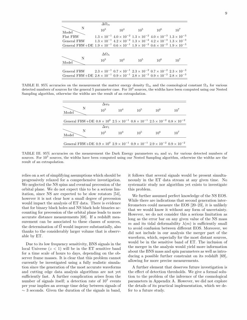
∆Ωm

ModelN

103 104 105 106 107

Flat FRW 1.3 × 10−1 4.0 × 10−2 1.3 × 10−2 4.0 × 10−3 1.3 × 10−3

General FRW 1.3 × 10−1 4.2 × 10−2 1.3 × 10−2 4.2 × 10−3 1.3 × 10−3

General FRW+DE 1.9 × 10−1 0.6 × 10−1 1.9 × 10−2 0.6 × 10−2 1.9 × 10−3

∆ΩΛ

ModelN

103 104 105 106 107

General FRW 2.3 × 10−1 0.7 × 10−1 2.3 × 10−2 0.7 × 10−2 2.3 × 10−3

General FRW+DE 2.8 × 10−1 0.9 × 10−1 2.8 × 10−2 0.9 × 10−2 2.8 × 10−3

TABLE II. 95% accuracies on the measurement the matter energy density Ωm and the cosmological constant ΩΛ for variousdetected numbers of sources for the general 5 parameter case. For 103 sources, the widths have been computed using our NestedSampling algorithm, otherwise the widths are the result of an extrapolation.

∆w0

ModelN

103 104 105 106 107

General FRW+DE 0.8 × 100 2.5 × 10−1 0.8 × 10−1 2.5 × 10−2 0.8 × 10−2

∆w1

ModelN

103 104 105 106 107

General FRW+DE 0.9 × 100 2.9 × 10−1 0.9 × 10−1 2.9 × 10−2 0.9 × 10−2

TABLE III. 95% accuracies on the measurement the Dark Energy parameters w0 and w1 for various detected numbers ofsources. For 103 sources, the widths have been computed using our Nested Sampling algorithm, otherwise the widths are theresult of an extrapolation.

relies on a set of simplifying assumptions which should beprogressively relaxed for a comprehensive investigation.We neglected the NS spins and eventual precession of theorbital plane. We do not expect this to be a serious lim-itation, since NS are expected to be slow rotators [54],however it is not clear how a small degree of precessionwould impact the analysis of ET data. There is evidencethat for binary black holes and NS black hole binaries ac-counting for precession of the orbital plane leads to moreaccurate distance measurements [68]. If a redshift mea-surement can be associated to these classes of sources,

the determination of ~Ω would improve substantially, alsothanks to the considerably larger volume that is observ-able by ET.

Due to its low frequency sensitivity, BNS signals in thelocal Universe (z < 1) will be in the ET sensitive bandfor a time scale of hours to days, depending on the ob-server frame masses. It is clear that this problem cannotcurrently be investigated using a fully realistic simula-tion since the generation of the most accurate waveformsand cutting edge data analysis algorithms are not yetsufficiently fast. A further complication arises from thenumber of signals itself; a detection rate of 107 eventsper year implies an average time delay between signals of∼ 3 seconds. Given the duration of the signals in band,

it follows that several signals would be present simulta-neously in the ET data stream at any given time. Nosystematic study nor algorithm yet exists to investigatethis problem.

We further assumed perfect knowledge of the NS EOS.While there are indications that second generation inter-ferometers could measure the EOS [20–23], it is unlikelythat we would know it without any form of uncertainty.However, we do not consider this a serious limitation aslong as the error bar on any given value of the NS massm and its tidal deformability λ(m) is sufficiently smallto avoid confusion between different EOS. Moreover, wedid not include in our analysis the merger part of thewaveform, which, especially for the most distant sources,would be in the sensitive band of ET. The inclusion ofthe merger in the analysis would yield more informationabout the BNS mass and spin parameters as well as intro-ducing a possible further constraint on its redshift [69],allowing for more precise measurements.

A further element that deserves future investigation isthe effect of detection thresholds. We give a formal solu-tion to the problem of the inference of the cosmologicalparameters in Appendix A. However, we did not explorethe details of its practical implementation, which we de-fer to a future study.

10

0.64

0.68

0.72

0.76

0.80

H0/100km ·s−1 ·Mpc−1

0.2

0.3

0.4

0.5

0.6

Ωm 68%

95%

99%

0.2

0.3

0.4

0.5

0.6

Ωm

FIG. 4. Posterior distributions for h and Ωm obtained fromthe analysis of 1,000 BNS events for a flat universe (Ωk = 0)and no dark energy equation of state. In the one dimensionalposteriors the dashed lines indicate the 2.5%, 50% and 97.5%confidence levels. In the two dimensional posterior distribu-tion we show the 68%, 95% and 99% confidence regions. Onall panels the solid (blue) lines indicate the fiducial values.

We ignored the effects of the detector calibration un-certainties over the inference of the GW event parameters

as well their impact over the global inference of ~Ω. At theend of the first observing run of Advanced LIGO, typicalamplitude uncertainties (which is relevant for the deter-mination of DL) and phase uncertainties (relevant for theestimation of z) were estimated at ∼ 10% and 10 degrees,respectively [70]. Simulations indicate that ignoring thepresence of such calibration errors does not lead to signifi-cant bias in the estimation of the GW parameters, as longas the SNR is not very large [71]. However, data analysismodels for GW analysis that marginalise over calibrationuncertainties are now available [72] and routinely utilisedfor the actual analysis [10]. The additional calibrationuncertainty increase the statistical uncertainty of the in-ferred parameters by a similar amount. In our case, thelargest source of uncertainty would come from the ampli-tude calibration and thus on the determination of DL forthe GW sources. Assuming, naively, an ET uncertaintybudget of ∼ 10%, we estimate a similar degradation of

our inference over ~Ω.

We also ignored the effects of weak lensing. Weak lens-ing is a zero mean process [73], thus, when averaging overthousands of sources, it will not induce an overall bias in

the estimate of ~Ω. A proper account of the lensing uncer-tainty, would lead to similar conclusions as the detectorcalibration uncertainty.

Even with the caveats discussed above, our studyshows that even considering exclusively information com-ing from GW alone (with no input from any EM asso-ciation) ET is capable to fully probe the evolution of

the Universe and determine the value of ~Ω with reason-able accuracy. We emphasise that our results apply to

a pure GW-based inference of ~Ω. A more accurate de-

termination of ~Ω from GW-EM joint detections may bepossible, thus the results presented in this study shouldbe regarded as a lower-limit to what the actual poten-tiality of ET is as a cosmological probe. Nevertheless, weshowed that GW alone can be a feasible complementaryand cross-validating route to probe the dynamics of theUniverse.

ACKNOWLEDGMENTS

This work benefitted from stimulating discussions andcomments from Bangalore Sathyaprakash, Alberto Vec-chio, John Veitch, Ilya Mandel and Christopher Berry.We thank the anonymous referees for their commentsand suggestions. The work was funded in part by a Lev-erhulme Trust research project grant. WDP is funded bythe program “Rientro dei Cervelli Rita Levi Montalcini”.

Appendix A: Inference of the cosmologicalparameters in presence of censored data

We want to infer the value of the cosmological param-

eters ~Ω ≡ (H0,Ωm,ΩΛ, . . .) given a set of gravitationalwaves observations. Consider a catalogue of gravitationalwave events E ≡ ε1, . . . , εN. Each event is defined as astretch of data di(t) given by the sum of noise ni(t) and a

gravitational wave signal hi(~Θ; t), where ~Θ indicates theset of all parameters of the signal and such that the SNRρ is greater than a given threshold ρth.

The likelihood to observe the event εi is given by

p(εi|~Θ,S, ρth, I) where S is the signal model that relates

the signal parameters ~Θ to a gravitational wave signalh. The posterior distribution for the parameters in oursignal model S comes from the application of Bayes’ the-orem

p(~Θ|εi,S, ρth, I) ∝ p(~Θ|S, I)p(εi|~Θ,S, ρth, I) (A1)

where p(~Θ|S, I) is the prior probability distribution for

the parameters ~Θ. Given a certain cosmic coalescence

rateR(~Ω, z), there will be a certain numberM ≡M(~Ω, z)of gravitational wave events that will not be registered asevents since their SNR will be below the selected thresh-old. Nevertheless, they encode information regarding theUniverse and they must be taken into account in our in-ference. The likelihood L−k for a non-detected event ε−k

11

0.15

0.30

0.45

Ωm

68%

95%

99%

0.64

0.68

0.72

0.76

H0 /100km ·s−1 ·Mpc−1

0.2

0.4

0.6

0.8

ΩΛ

68%

95%

99%

0.15

0.30

0.45

Ωm

68%

95%

99%

0.2

0.4

0.6

0.8

ΩΛ

FIG. 5. Same as Fig. 4, but for a general FRWL universe.

is given by

L−k (ε−k , ρth) ≡ p(ε−k |~Ω, R(~Ω, z), ρth, I) (A2)

=

∫ ρth

0

p(ε−k , ρk|~Ω, R(~Ω, z), ρth, I)dρk .

(A3)

For a set of M non-detected events, the likelihood willbe given by

L−(ε−, ρth) =

M∏k=1

L−k (ε−k , ρth) (A4)

=[L−k (ε−k , ρth)

]M(A5)

The number of non-detected events M(~Ω, z) is a nui-

sance parameters which depends on ~Ω, the rate R(~Ω, z),the detection threshold ρth, the observation time T and

the observed volume V (~Ω, ρth) as

M(~Ω, z) = R(~Ω, z)V (~Ω, ρth)T −N . (A6)

We are now in the position of writing the posterior dis-

tribution for the cosmological parameters ~Ω:

12

0.00

0.15

0.30

0.45

Ωm

68%

95%

99%

99%

0.2

0.4

0.6

0.8

ΩΛ

68%

95%

99%

99%

99%

68%

95%99%

1.6

1.2

0.8

0.4

0.0

w0 68%

95%

99%

99%

68%

95%

99%

99%

68%95

%

99%99

%

99%

0.60

0.65

0.70

0.75

0.80

H0/100km ·s−1 ·Mpc−1

1.0

0.5

0.0

0.5

1.0

w1

68%

95%

95%

99%99

%

0.00

0.15

0.30

0.45

Ωm

68%

95% 95%

99%

99%

99%

0.2

0.4

0.6

0.8

ΩΛ

68%

95%

95%

99%

99%

1.6

1.2

0.8

0.4

0.0

w0

68%

95%

95%

99%

99%

99%

1.0

0.5

0.0

0.5

1.0

w1

FIG. 6. Same as Fig. 4, but for a general FRWL universe + DE parameters.

p(~Ω|E , N, ρth, S, I) ∝ p(~Ω|S, I)∫ Rmax(~Ω,z)

0

dR(~Ω, z) p(R(~Ω, z)|~Ω, S, I)N∏i=1

L(εi, ~Ω)

∞∑M=0

[L−k (ε−k , ρth)

]Mp(M |~Ω, R(~Ω, z), ρth) .

(A7)

It is interesting to verify that Eq. (A7) reduces toEq. (10) in the limit of ρth → 0. In this limit we have

also

M → 0 (A8)

p(M |~Ω, R(~Ω, z), ρth)→ δM,0 (A9)∫ ρth

0

p(ε−k , ρk|~Ω, R(~Ω, z), ρth, I)dρk → 0 (A10)

13

therefore the term[L−k (ε−k , ρth)

]M → 1 (A11)

and the non-detection part of the likelihood reduces to

∞∑M=0

δM,0 = 1 . (A12)

Assuming that the rate R(~Ω, z) is given by the integralof Eq. (12), we recover the form of the likelihood (10)which we used in our study.

[1] http://www.ligo.caltech.edu/advLIGO/ ().[2] B. P. Abbott et al. (LIGO Scientific Collaboration,

Virgo Collaboration), Physical Review Letters 116,131103 (2016), https://dcc.ligo.org/LIGO-P1500237/public/main, arXiv:1602.03838 [gr-qc].

[3] http://wwwcascina.virgo.infn.it/advirgo/ ().[4] K. Kuroda and LCGT Collaboration, Classical and

Quantum Gravity 27, 084004 (2010).[5] C. S. Unnikrishnan, International Journal of Modern

Physics D 22, 1341010 (2013).[6] B. P. Abbott et al. (LIGO Scientific Collaboration, Virgo

Collaboration), Physical Review Letters 116, 061102(2016), https://dcc.ligo.org/LIGO-P150914/public/

main, arXiv:1602.03847 [gr-qc].[7] B. P. Abbott et al. (LIGO Scientific Collaboration and

Virgo Collaboration), Phys. Rev. Lett. 116, 241103(2016).

[8] B. P. Abbott, R. Abbott, T. D. Abbott, M. R. Aber-nathy, F. Acernese, K. Ackley, C. Adams, T. Adams,P. Addesso, R. X. Adhikari, and et al., Physical ReviewX 6, 041015 (2016).

[9] B. P. Abbott et al. (LIGO Scientific Collaboration,Virgo Collaboration), (2016), https://dcc.ligo.org/

LIGO-P1500213/public/main, arXiv:1602.03841 [gr-qc].[10] B. P. Abbott et al. (LIGO Scientific Collaboration,

Virgo Collaboration), (2016), https://dcc.ligo.org/

LIGO-P1500218/public/main, arXiv:1602.03840 [gr-qc].[11] B. P. Abbott et al. (LIGO Scientific Collabora-

tion, Virgo Collaboration), Astrophysical Journal 818,L22 (2016), https://dcc.ligo.org/LIGO-P1500262/

public/main, arXiv:1602.03846 [astro-ph.HE].[12] B. P. Abbott et al. (LIGO Scientific Collaboration,

Virgo Collaboration), (2016), https://dcc.ligo.org/

LIGO-P1500217/public/main, arXiv:1602.03842 [astro-ph.HE].

[13] J. Abadie, B. P. Abbott, R. Abbott, M. Abernathy,T. Accadia, F. Acernese, C. Adams, R. Adhikari,P. Ajith, B. Allen, and et al., Phys. Rev. D 82, 102001(2010), arXiv:1005.4655 [gr-qc].

[14] W. Del Pozzo, J. Veitch, and A. Vecchio, Phys. Rev. D83, 082002 (2011), arXiv:1101.1391 [gr-qc].

[15] T. G. F. Li, W. Del Pozzo, S. Vitale, C. Van Den Broeck,M. Agathos, J. Veitch, K. Grover, T. Sidery, R. Stu-rani, and A. Vecchio, Phys. Rev. D 85, 082003 (2012),arXiv:1110.0530 [gr-qc].

[16] N. Cornish, L. Sampson, N. Yunes, and F. Pretorius,Phys. Rev. D 84, 062003 (2011), arXiv:1105.2088 [gr-qc].

[17] S. Nissanke, D. E. Holz, S. A. Hughes, N. Dalal, and J. L.Sievers, ApJ 725, 496 (2010), arXiv:0904.1017 [astro-ph.CO].

[18] W. Del Pozzo, Phys. Rev. D 86, 043011 (2012),arXiv:1108.1317 [astro-ph.CO].

[19] S. R. Taylor, J. R. Gair, and I. Mandel, Phys. Rev. D85, 023535 (2012), arXiv:1108.5161 [gr-qc].

[20] J. S. Read, C. Markakis, M. Shibata, K. Uryu, J. D. E.Creighton, and J. L. Friedman, Phys. Rev. D 79, 124033(2009), arXiv:0901.3258 [gr-qc].

[21] T. Hinderer, B. D. Lackey, R. N. Lang, and J. S. Read,Phys. Rev. D 81, 123016 (2010), arXiv:0911.3535 [astro-ph.HE].

[22] B. D. Lackey, K. Kyutoku, M. Shibata, P. R. Brady,and J. L. Friedman, Phys. Rev. D 89, 043009 (2014),arXiv:1303.6298 [gr-qc].

[23] W. Del Pozzo, T. G. F. Li, M. Agathos, C. Van DenBroeck, and S. Vitale, Physical Review Letters 111,071101 (2013), arXiv:1307.8338 [gr-qc].

[24] M. Abernathy et al., Einstein gravitational wave Tele-scope conceptual design study , Tech. Rep. ET-0106A-10(2011).

[25] A. Freise, S. Chelkowski, S. Hild, W. Del Pozzo, A. Per-reca, and A. Vecchio, Classical and Quantum Gravity26, 085012 (2009), arXiv:0804.1036 [gr-qc].

[26] M. Punturo, M. Abernathy, F. Acernese, B. Allen,N. Andersson, K. Arun, F. Barone, B. Barr, M. Bar-suglia, M. Beker, N. Beveridge, S. Birindelli, S. Bose,L. Bosi, S. Braccini, C. Bradaschia, T. Bulik, E. Cal-loni, G. Cella, E. Chassande Mottin, S. Chelkowski,A. Chincarini, J. Clark, E. Coccia, C. Colacino, J. Co-las, A. Cumming, L. Cunningham, E. Cuoco, S. Danil-ishin, K. Danzmann, G. De Luca, R. De Salvo, T. Dent,R. De Rosa, L. Di Fiore, A. Di Virgilio, M. Doets,V. Fafone, P. Falferi, R. Flaminio, J. Franc, F. Fras-coni, A. Freise, P. Fulda, J. Gair, G. Gemme, A. Gennai,A. Giazotto, K. Glampedakis, M. Granata, H. Grote,G. Guidi, G. Hammond, M. Hannam, J. Harms,D. Heinert, M. Hendry, I. Heng, E. Hennes, S. Hild,J. Hough, S. Husa, S. Huttner, G. Jones, F. Khalili,K. Kokeyama, K. Kokkotas, B. Krishnan, M. Lorenzini,H. Luck, E. Majorana, I. Mandel, V. Mandic, I. Mar-tin, C. Michel, Y. Minenkov, N. Morgado, S. Mosca,B. Mours, H. Muller-Ebhardt, P. Murray, R. Nawrodt,J. Nelson, R. Oshaughnessy, C. D. Ott, C. Palomba,A. Paoli, G. Parguez, A. Pasqualetti, R. Passaqui-eti, D. Passuello, L. Pinard, R. Poggiani, P. Popolizio,M. Prato, P. Puppo, D. Rabeling, P. Rapagnani, J. Read,T. Regimbau, H. Rehbein, S. Reid, L. Rezzolla, F. Ricci,F. Richard, A. Rocchi, S. Rowan, A. Rudiger, B. Sasso-las, B. Sathyaprakash, R. Schnabel, C. Schwarz, P. Sei-del, A. Sintes, K. Somiya, F. Speirits, K. Strain, S. St-rigin, P. Sutton, S. Tarabrin, A. Thuring, J. van den

14

Brand, C. van Leewen, M. van Veggel, C. van den Broeck,A. Vecchio, J. Veitch, F. Vetrano, A. Vicere, S. Vy-atchanin, B. Willke, G. Woan, P. Wolfango, and K. Ya-mamoto, Classical and Quantum Gravity 27, 194002(2010).

[27] B. F. Schutz, Nature 323, 310 (1986).[28] B. S. Sathyaprakash and B. F. Schutz, Living Reviews in

Relativity 12, 2 (2009), arXiv:0903.0338 [gr-qc].[29] E. Nakar, A. Gal-Yam, and D. B. Fox, arXiv.org (2005),

astro-ph/0511254v2.[30] B. S. Sathyaprakash, B. F. Schutz, and C. Van Den

Broeck, Classical and Quantum Gravity 27, 215006(2010), arXiv:0906.4151 [astro-ph.CO].

[31] W. Zhao, C. van den Broeck, D. Baskaran, and T. G. F.Li, Phys. Rev. D 83, 023005 (2011), arXiv:1009.0206[astro-ph.CO].

[32] S. Nissanke, D. E. Holz, N. Dalal, S. A. Hughes, J. L.Sievers, and C. M. Hirata, ArXiv e-prints (2013),arXiv:1307.2638 [astro-ph.CO].

[33] B. D. Metzger, G. Martınez-Pinedo, S. Darbha,E. Quataert, A. Arcones, D. Kasen, R. Thomas, P. Nu-gent, I. V. Panov, and N. T. Zinner, MNRAS 406, 2650(2010), arXiv:1001.5029 [astro-ph.HE].

[34] M. Tanaka, Advances in Astronomy 2016, 634197(2016), arXiv:1605.07235 [astro-ph.HE].

[35] K. Belczynski, R. O’Shaughnessy, V. Kalogera, F. Ra-sio, R. E. Taam, and T. Bulik, ApJ 680, L129 (2008),arXiv:0712.1036.

[36] C. L. MacLeod and C. J. Hogan, Phys. Rev. D 77, 043512(2008), arXiv:0712.0618.

[37] A. Petiteau, S. Babak, and A. Sesana, ApJ 732, 82(2011), arXiv:1102.0769 [astro-ph.CO].

[38] S. R. Taylor and J. R. Gair, Phys. Rev. D 86, 023502(2012), arXiv:1204.6739 [astro-ph.CO].

[39] B. Sathyaprakash et al., ArXiv e-prints (2011),arXiv:1108.1423 [gr-qc].

[40] C. Messenger and J. Read, Physical Review Letters 108,091101 (2012), arXiv:1107.5725 [gr-qc].

[41] T. G. F. Li, W. Del Pozzo, and C. Messenger, ArXive-prints (2013), arXiv:1303.0855 [gr-qc].

[42] B. P. Abbott, R. Abbott, T. D. Abbott, M. R. Aber-nathy, K. Ackley, C. Adams, P. Addesso, R. X. Adhikari,V. B. Adya, C. Affeldt, and et al., ArXiv e-prints (2016),arXiv:1607.08697 [astro-ph.IM].

[43] E. T. Jaynes, Probability theory: the logic of science(Cambridge university press, 2003).

[44] https://www.lsc-group.phys.uwm.edu/daswg/

projects/lalsuite.html ().[45] B. Kiziltan, A. Kottas, and S. E. Thorsett, in American

Astronomical Society Meeting Abstracts #215, Bulletinof the American Astronomical Society, Vol. 42 (2010) p.300.08.

[46] H. Muller and B. D. Serot, Nuclear Physics A 606, 508(1996), nucl-th/9603037.

[47] B. D. Lackey, M. Nayyar, and B. J. Owen, Phys. Rev. D73, 024021 (2006), astro-ph/0507312.

[48] M. Prakash, J. R. Cooke, and J. M. Lattimer,Phys. Rev. D 52, 661 (1995).

[49] D. M. Coward and R. R. Burman, MNRAS 361, 362(2005), astro-ph/0505181.

[50] D. W. Hogg, ArXiv Astrophysics e-prints (1999), astro-

ph/9905116.[51] E. V. Linder, Physical Review Letters 90, 091301 (2003),

astro-ph/0208512.[52] T. Regimbau, T. Dent, W. Del Pozzo, S. Giampa-

nis, T. G. F. Li, C. Robinson, C. Van Den Broeck,D. Meacher, C. Rodriguez, B. S. Sathyaprakash,and K. Wojcik, Phys. Rev. D 86, 122001 (2012),arXiv:1201.3563 [gr-qc].

[53] C. Messenger and J. Veitch, New Journal of Physics 15,053027 (2013), arXiv:1206.3461 [astro-ph.IM].

[54] R. O’Shaughnessy, C. Kim, V. Kalogera, and K. Bel-czynski, ApJ 672, 479 (2008), astro-ph/0610076.

[55] A. Buonanno, B. R. Iyer, E. Ochsner, Y. Pan, andB. S. Sathyaprakash, Phys. Rev. D 80, 084043 (2009),arXiv:0907.0700 [gr-qc].

[56] C. K. Mishra, K. G. Arun, B. R. Iyer, andB. S. Sathyaprakash, Phys. Rev. D 82, 064010 (2010),arXiv:1005.0304 [gr-qc].

[57] C. Markakis, J. S. Read, M. Shibata, K. Uryu, J. D. E.Creighton, and J. L. Friedman, ArXiv e-prints (2010),arXiv:1008.1822 [gr-qc].

[58] T. Damour, A. Nagar, and L. Villain, Phys. Rev. D 85,123007 (2012), arXiv:1203.4352 [gr-qc].

[59] S. Hild, S. Chelkowski, and A. Freise, ArXiv e-prints(2008), arXiv:0810.0604 [gr-qc].

[60] J. Skilling, in American Institute of Physics ConferenceSeries, Vol. 735 (2004) pp. 395–405.

[61] J. Veitch and A. Vecchio, Phys. Rev. D 81, 062003(2010), arXiv:0911.3820 [astro-ph.CO].

[62] T. S. Ferguson, The annals of statistics , 209 (1973).[63] N. L. Hjort, C. Holmes, P. Muller, and S. G. Walker,

AMC 10, 12 (2010).[64] D. M. Blei, M. I. Jordan, et al., Bayesian analysis 1, 121

(2006).[65] http://code.google.com/p/haines/wiki/dpgmm ().[66] Planck Collaboration, P. A. R. Ade, N. Aghanim, M. Ar-

naud, M. Ashdown, J. Aumont, C. Baccigalupi, A. J.Banday, R. B. Barreiro, J. G. Bartlett, and et al., ArXive-prints (2015), arXiv:1502.01589.

[67] Planck Collaboration, P. A. R. Ade, N. Aghanim, M. Ar-naud, M. Ashdown, J. Aumont, C. Baccigalupi, A. J.Banday, R. B. Barreiro, N. Bartolo, and et al., ArXive-prints (2015), arXiv:1502.01590.

[68] S. Vitale, R. Lynch, J. Veitch, V. Raymond, andR. Sturani, Physical Review Letters 112, 251101 (2014),arXiv:1403.0129 [gr-qc].

[69] C. Messenger, K. Takami, S. Gossan, L. Rezzolla,and B. S. Sathyaprakash, ArXiv e-prints (2013),arXiv:1312.1862 [gr-qc].

[70] B. P. Abbott et al. (LIGO Scientific Collabora-tion), (2016), https://dcc.ligo.org/LIGO-P1500248/public/main, arXiv:1602.03845 [gr-qc].

[71] S. Vitale, W. Del Pozzo, T. G. F. Li, C. Van Den Broeck,I. Mandel, B. Aylott, and J. Veitch, Phys. Rev. D 85,064034 (2012), arXiv:1111.3044 [gr-qc].

[72] W. M. Farr, B. Farr, and T. Littenberg, Tech. Rep.(2015).

[73] M. Bartelmann and P. Schneider, Phys. Rep. 340, 291(2001), astro-ph/9912508.