Starting School at Four: The Effect of Universal Pre ... · Fitzpatrick: Starting School at Four Published by The Berkeley Electronic Press, 2008. year, approximately 55 percent (75,299)

This work is distributed as a Discussion Paper by the

STANFORD INSTITUTE FOR ECONOMIC POLICY RESEARCH

SIEPR Discussion Paper No. 08-05

Starting School at Four: The Effect of Universal Pre-Kindergarten

on Children’s Academic Achievement

By Maria Donovan Fitzpatrick

Stanford University

December 2008

Stanford Institute for Economic Policy Research

Stanford University Stanford, CA 94305

(650) 725-1874 The Stanford Institute for Economic Policy Research at Stanford University supports research bearing on economic and public policy issues. The SIEPR Discussion Paper Series reports on research and policy analysis conducted by researchers affiliated with the Institute. Working papers in this series reflect the views of the authors and not necessarily those of the Stanford Institute for Economic Policy Research or Stanford University.

The B.E. Journal of EconomicAnalysis & Policy

AdvancesVolume 8, Issue 1 2008 Article 46

Starting School at Four: The Effect ofUniversal Pre-Kindergarten on Children’s

Academic Achievement

Maria D. Fitzpatrick∗

∗SIEPR, Stanford University, [email protected]

Recommended CitationMaria D. Fitzpatrick (2008) “Starting School at Four: The Effect of Universal Pre-Kindergartenon Children’s Academic Achievement,” The B.E. Journal of Economic Analysis & Policy: Vol. 8:Iss. 1 (Advances), Article 46.Available at: http://www.bepress.com/bejeap/vol8/iss1/art46

Copyright c©2008 The Berkeley Electronic Press. All rights reserved.

Starting School at Four: The Effect ofUniversal Pre-Kindergarten on Children’s

Academic Achievement∗

Maria D. Fitzpatrick

Abstract

Universal Pre-Kindergarten (Pre-K) programs differ from widely known and extensively eval-uated programs like Head Start and Perry Preschool because access is open to all children of theappropriate age. To estimate the intent-to-treat effects of these programs on the long term educa-tional achievement of children, I use a differences-in-differences framework and individual-leveldata from the National Assessment of Educational Progress. For disadvantaged children residingin small towns and rural areas, Universal Pre-K availability increases both reading and mathe-matics test scores at fourth grade as well as the probability of students being on-grade for theirage. Increases in some measures of achievement also were seen among other groups, though thepatterns were less uniform across outcome measures. The results correspond with other workshowing children living in less densely populated areas are those most likely to enroll in preschoolbecause of the program’s availability.

KEYWORDS: human capital, state and federal aid, early childhood education

∗SIEPR, Stanford University. Mail: 579 Serra Mall at Galvez St., Stanford CA 94305. e-mail:[email protected]. This research was supported by the Institute of Education Sciences U.S.Department of Education Award #R305B040049. Additional funding was provided by the SpencerFoundation and the Bankard Fund for Political Economy. Special thanks to Al Rogers and SteveGorman for their help with the NAEP data. This paper has greatly benefited from the helpfulcomments of Leora Friedberg, Caroline Hoxby, William R. Johnson, Amalia R. Miller, John Pep-per, Sarah E. Turner, two anonymous referees and the participants at the Center for the AdvancedStudy of Teaching and Learning Workshop at the University of Virginia. All errors are my own.

I. Introduction Publicly subsidized Pre-Kindergarten (Pre-K) programs have received considerable attention in recent years as an avenue for providing child care and promoting school readiness. Almost 40 states currently fund Pre-K programs; over 800,000 children were enrolled nationwide in 2004-2005.1 Compared to just a decade earlier, this is more than a twofold increase in the number of children in state subsidized preschool.2 Most of the ongoing programs target children in low-income families. However, three states (Georgia, Oklahoma and Florida) have introduced universal public preschool programs. The recent expansion of and interest in early childhood education programs stems largely from the widely advertised success of a few model programs, including the Abecedarian and Perry Preschool studies, which generally provided large-scale multidimensional packages of interventions to very low-income families. While the long-term success of these interventions at improving life outcomes of participating children has been widely accepted, the programs were costly at anywhere from $16,000 to $41,000 per child..3 Such costs are too high for state governments to fund similar intensive interventions for all residents. (In contrast, the Georgia Pre-K program spent $4,010 per student in 2007, albeit for a much larger number of children.4) Policymakers today therefore face a trade-off: provide comprehensive intensive early childhood interventions targeted at disadvantaged children or institute smaller-scale education-based Universal Pre-K programs. Crucial to making a correct choice is an understanding of the long-term effects of Universal Pre-K programs. To date, there has been little evidence on the long-term effects of Universal Pre-K on children's outcomes, so much of the discussion of potential benefits has involved extrapolating from estimated benefits of the smaller intensive interventions targeted at disadvantaged students to the entire population. However, early childhood education opportunities of all children absent government intervention are not the same and much of the expenditure on a universal program is spent on children who would enroll in preschool or have high-quality at-home-care (Fitzpatrick 2008). It is therefore unlikely that all students will have the same potential to gain from Universal Pre-K programs.

1 http://nieer.org/yearbook/pdf/yearbook.pdf .(Accessed July 25, 2006) 2 http://www.ecs.org/html/IssueSection.asp?issueid=184&s=Quick+Facts. (Accessed July 25, 2006) 3 Cost estimates are based on estimates from Fuller (2007) and have been updated to 2007 U.S. dollars. 4 Cost estimates of Georgia Pre-K expenditures are from the Southern Education Foundation, www.southerneducation.org/pdf/Ga%20Pre-K%20Report-Final.pdf.

1

Fitzpatrick: Starting School at Four

Published by The Berkeley Electronic Press, 2008

In this analysis, I use individual-level data from the National Assessment of Educational Progress (NAEP) to estimate the effects of the availability of Universal Pre-K for four year olds on test scores and progression through school as of the fourth grade. Measuring the effects of these programs on test scores is important as researchers have shown that higher test scores are related to increased wages, even after accounting for years of schooling (Murnane et al. 1995). However, researchers also have suggested that high-quality preschool programs have positive impacts on longer term outcomes such as wages and criminal activity despite their not having permanently increased test scores (Schweinhart et al. 1993). Perhaps these programs have effects on non-cognitive as well as cognitive skills. Progression through school may involve more display of non-cognitive skill than test taking, so I also investigate whether the availability of Universal Pre-K in Georgia had any affect on-grade retention. Changes over time (comparison with children from earlier cohorts lacking universal eligibility) and variation across states (Georgia versus those without Universal Pre-K) identify the effects of Universal Pre-K. The key identifying assumption is that other factors affecting achievement did not change concurrently for students in Georgia relative to other students. I explore the robustness of the results to this assumption in a number of specifications, such as including eighth graders as an additional control group. In addition, the analysis allows for differential effects of the program on children from different race and socio-economic status groups.

Though estimates showing statewide gains in math test scores and the probability of being on-grade are not robust to specification choice, there are gains in the academic achievement of some groups of children. Specifically, disadvantaged children living in small towns and rural areas show increases in math and reading scores of up to 12 percent of a standard deviation because of Universal Pre-K availability. These children also appear to be slightly more likely to be on-grade for their age. Statistically significant gains for other groups of children also are seen on some, but not all, of the measures of academic achievement, which leads to caution in making any conclusions for these other groups. Findings that Universal Pre-K availability increased the academic achievement of children in urban fringe and rural areas corresponds with other research showing that these areas see the largest increases in preschool enrollment due to the program’s availability.

The next section of the paper describes the Universal Pre-K program and offers a summary of the literature on the effects of early childhood interventions on test scores and grade retention. The empirical strategy is outlined in section III. Section IV gives an overview of the data used in the analysis. Results are presented in section V and Section VI concludes.

2

The B.E. Journal of Economic Analysis & Policy, Vol. 8 [2008], Iss. 1 (Advances), Art. 46

http://www.bepress.com/bejeap/vol8/iss1/art46

Figure 1. Percent of Four Year Olds in Georgia Enrolled in the Georgia Pre-K Program

7.8%

13.9%

38.8%

50.5% 51.8% 53.0%

0%

10%

20%

30%

40%

50%

60%

FY94FY95

FY96FY97

FY98FY99

Georgia program means-tested

Georgia program becomes universal

Notes: From Brackett et al. (1999). A fiscal year runs from October of the previous year to September of the year in its name. For example, FY96 runs from October 1, 1995 to September 30, 1996. Percent of population of four year olds is calculated using the Census Bureau’s Time Series of State Population Estimates by Age, which can be found at http://www.census.gov/popest/archives/1990s/st_age_sex.html.

II. Background and Evidence II.a. Georgia Pre-Kindergarten In 1993, Georgia instituted a lottery which funded a Pre-K program for four year olds.5 It was initially available only to low- to middle-income households. In the first year households with income below $66,000 were eligible and in the second year households with income below $100,000 were eligible. Because of an unexpected surplus of funds, the program expanded in the Fall of 1995 to include all age-eligible state residents. Figure 1 shows the increase in the number of children enrolled during the program’s early years.6 By the 2007-2008 school- 5 Though part of the same legislation and funded by the same lottery, Georgia’s HOPE scholarship program has received considerably more attention than Universal Pre-K, particularly academic, and has been the focus of many scholarly articles, e.g. Dynarksi (2000) and Long (2004). 6 Numbers in this section were converted from totals to percents and vice versa using the U.S. Census Bureau’s population estimates for the corresponding year. These estimates can be found at http://www.census.gov/popest/estimates.php. (Accessed July 25, 2006)

3



year, approximately 55 percent (75,299) of four year olds were enrolled in Georgia Pre-Kindergarten (GPK) at a total state cost of $302 million, which translates to $4,010 per student per year and $3.43 per child per hour of care.7

GPK is voluntary, free, and available to all children who turn four by September 1 of the school year, regardless of family income. Universal Pre-K classes are provided by a wide range of approved facilities, including public schools, Head Start centers, private child care centers, faith-based and other non-profit centers. Programs run five days a week for the length of the school year for the state-mandated 6.5 hour day.8 Teachers and classroom assistants are required to meet different educational requirements than those for non-Pre-K centers.9 In GPK, a minimum staff to child ratio of 1:10 is imposed and a maximum of 20 students are allowed to be enrolled in a classroom. In addition, providers may choose to follow one of several approved curricula.10 The state of Georgia transfers lottery funds directly to centers.

II.b. Evidence on Universal Early Childhood Interventions While early childhood education has been the focus of much research, including that of economists (see Currie and Thomas 1995, 1999; Blau and Currie, 2004; Magnuson et al. 2004), little evidence has been gathered about how the availability and take-up of Universal Pre-K programs affects attainment. Such programs are different from regular preschool or day care programs in many ways that can be expected to influence their effect on children. For example, as described above, the Universal Pre-K programs analyzed here impose higher teacher standards, stronger curricula guidelines and lower child-to-staff ratios than typically set by state governments for other licensed child care centers. In addition, the programs include a broader set of participants than those involved in other widely studied interventions, such as Head Start or the Perry Preschool Project. Children from various backgrounds can be expected to respond to an intervention differently, in part because they would have different care

7 Cost estimates of Georgia Pre-K expenditures are from the Southern Education Foundation, www.southerneducation.org/pdf/Ga%20Pre-K%20Report-Final.pdf. 8 Centers are encouraged to offer additional care (after set program hours and during the summer). The cost of this ‘supplemental care’ is not covered by the state, though it is capped for low-income participants. 9 Non-Pre-K centers include all preschools, nursery schools and child care centers. This is because, in general, state provisions about quality only use age as the dimension along which to determine requirements. They do not distinguish between child care (a place that basically just watches children) and preschool (a place that focuses on educational instruction). 10 Rules for centers in Georgia not receiving state money for Pre-K are a staff-child ratio of at least 1:18, maximum group size of 36, and no minimum educational requirement for teachers or assistants.

4



alternatives in the absence of the program. Therefore, it is important to evaluate the distinct effects of Universal Pre-K on the whole population of children. In fact, support for this can be seen in Barnett’s reviews (1995, 1998) of the literature, in which he finds large public programs generally have weaker long term impacts on children’s academic achievement than smaller, higher quality, more targeted programs.11 In 2001, researchers began the Early Childhood Study to examine the effects of participating in the GPK on the academic outcomes of children in the state. In their report from the study, Henry et al. (2003) compare children who attended GPK to those in Georgia Head Start and private preschool programs. They find children in GPK show at least as much improvement over the course of the year as those in private preschools and about the same amount of improvement as children in Georgia’s Head Start programs. This is a strict comparison of “gains scores”, though, and the results should be interpreted with caution in case there are systematic differences in the characteristics of families and children attending various types of preschool programs that are correlated with their increases in achievement. Gormley and Gayer (2005) and Gormley et al. (2005) analyze the effect of the Oklahoma Pre-K program on students in Tulsa. They begin by comparing test scores of kindergarteners who participated in Oklahoma Pre-K to those who did not. However, any analyses of the effects of enrollment might be plagued by selection bias – those who enroll may be those who will see the largest benefit to doing so. In order to control for potential selection bias the authors also compare test scores of children in kindergarten who participated in the prior year to test scores of children just beginning their participation in Oklahoma Pre-K (who are arguably similar in both observable and unobservable characteristics to their counterparts in the earlier cohort). Their results suggest test scores increased by 0.24 to 0.39 standard deviations, depending on the test subject. In addition, they found the largest gains in test scores were for Hispanics and African-Americans, while white children showed little improvement. The generalizability of their results may be limited, given that their sample only includes children in Tulsa. Additionally, their estimates are of the effects of the treatment on the treated, while those presented in the current work are intention to treat effects. Understanding program effects for enrolled children is important, but the policy question at hand is whether to make Pre-K programs available to all residents, not whether to lower the compulsory schooling age. 12 This paper is therefore better

11 It should be noted that although large scale public programs might not have as large effects on children as targeted programs, they may be more widely popular and therefore more likely survive the political system. 12 In most states even the kindergarten programs are voluntary, so it seems unlikely that the compulsory schooling age would jump from where it is now, at six or seven, to four.

5



suited to answer the current relevant policy question – whether the introduction of voluntary Universal Pre-K programs improves child outcomes. In some respects, the introduction of Universal Pre-K parallels the expansion of access to kindergarten in the 1960s and 1970s studied by Cascio (2004). Using variation in the timing of states' decisions to fund kindergarten programs in a differences-in-differences (D-D) framework, she finds the programs decreased grade retention (by high school) among whites by about 20 percent and among minorities of 30 to 40 percent. Cascio finds little effect of kindergarten availability on high school graduation. Though there are similarities between the kindergartens Cascio studies and Pre-K programs today, it is likely younger children would respond to such programs differently, as a year at such a young age can mean quite a bit in terms of the cognitive abilities of a child.13 Also, since the 1960s and 1970s there have been significant changes in our society (e.g. more women in the workforce) that might affect families’ responsiveness to child care subsidies. Additionally, although the effects of preschool programs may be long lasting (as educators hope and politicians promise), it may be the case that the gains to investing in early childhood education are not entirely borne out in high school graduation rates, as high school graduation happens much later in life and is likely the result of a combination of a myriad of factors.14

III. Empirical Strategy III.a. Test Scores The goal of this paper is to estimate the average effect of the availability of Universal Pre-K on academic achievement measured in fourth grade. To estimate this intent-to-treat effect, I use a D-D estimation strategy. Table 1 shows the type of Pre-K available to children in Georgia. The first column shows the Pre-K funding mechanism in place for children in preschool from 1990 to 2005. Using the table, cohorts of students can be tracked by following diagonally across the table as the students go from kindergarten through fourth grade. The seventh column of the table shows the type of Pre-K available in the state of Georgia to children in the fourth grade in the school year specified. The first students in

13 To illustrate, see the American Association of Pediatrics recommendations for developmental milestones of four year old and five year old children (2004). For example, while four year olds are on track if they are just beginning to count, five year olds should have understanding of general household items such as food, money, etc. 14 Garces et al. (2002) find that Head Start also has positive effects on long-term outcomes for participating children and their younger siblings. For example, whites who attended Head Start were significantly more likely to complete high school.

6



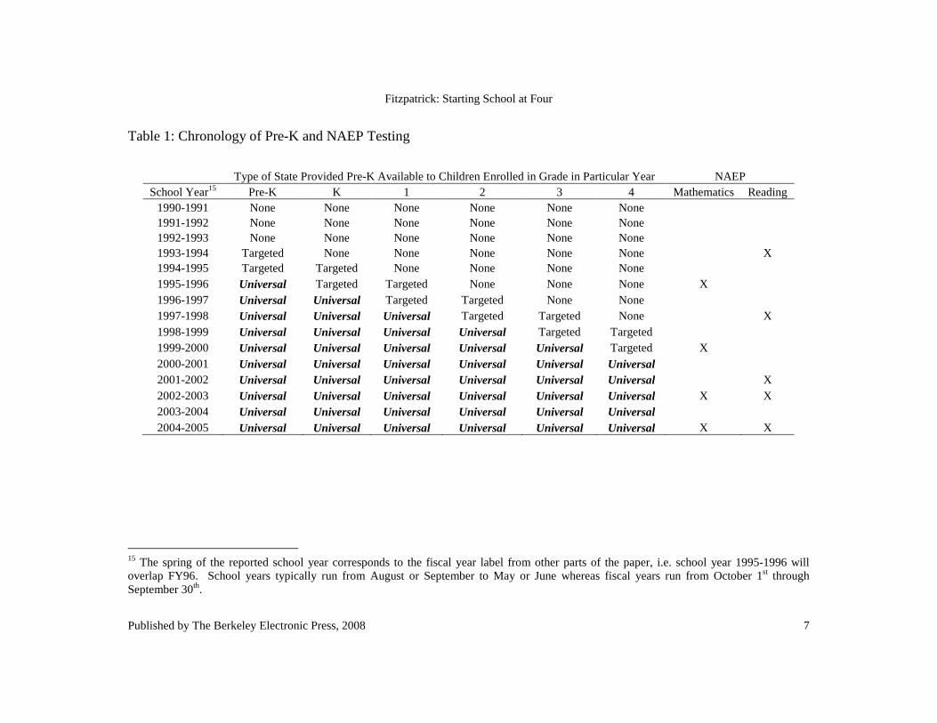
Table 1: Chronology of Pre-K and NAEP Testing

Type of State Provided Pre-K Available to Children Enrolled in Grade in Particular Year NAEP

School Year15 Pre-K K 1 2 3 4 Mathematics Reading 1990-1991 None None None None None None 1991-1992 None None None None None None 1992-1993 None None None None None None 1993-1994 Targeted None None None None None X 1994-1995 Targeted Targeted None None None None 1995-1996 Universal Targeted Targeted None None None X 1996-1997 Universal Universal Targeted Targeted None None 1997-1998 Universal Universal Universal Targeted Targeted None X 1998-1999 Universal Universal Universal Universal Targeted Targeted 1999-2000 Universal Universal Universal Universal Universal Targeted X 2000-2001 Universal Universal Universal Universal Universal Universal 2001-2002 Universal Universal Universal Universal Universal Universal X 2002-2003 Universal Universal Universal Universal Universal Universal X X 2003-2004 Universal Universal Universal Universal Universal Universal 2004-2005 Universal Universal Universal Universal Universal Universal X X

15 The spring of the reported school year corresponds to the fiscal year label from other parts of the paper, i.e. school year 1995-1996 will overlap FY96. School years typically run from August or September to May or June whereas fiscal years run from October 1st through September 30th.

7



Georgia eligible for GPK were age four by September 1, 1995 and, therefore, would have been in fourth grade in 2001. The State National Assessments of Educational Progress (NAEP) assessment (the only NAEP considered to be appropriate for analyses at the state level) is only offered every few years and until 2003 did not operate on a regular schedule. Table 1 also details the NAEP schedule of testing, allowing the reader to see when the NAEP was offered and what type of Pre-K the children in Georgia who took the NAEP had available to them at the time they were age eligible. Fourth graders in Georgia in the 2002-2003 school-year were the first group tested in math who had been eligible for Universal Pre-K; the first eligible group tested in reading was in fourth grade in Georgia in the 2001-2002 school year. The comparison is between fourth graders in Georgia who were program eligible to those who were not (both in all states and before program implementation in Georgia).16 The most parsimonious version of this linear D-D framework can be represented as

.ijttiitijt StateUPKY εθβα ++++= (1)

In (1), ijtY represents the standardized test score of student i at school j in period t.

State and year fixed effects are included; in the equation they are represented by

iState and tθ , respectively. itUPK is a dichotomous variable that takes on a value

of one if the child is a member of a cohort in fourth grade in Georgia after the 2000-2001 school year. β is therefore the estimate of the program effect. The key assumption is that there were no other concurrent changes specific to Georgia that affected the academic achievement of children other than the introduction of Universal Pre-K.

To be clear, the “pre-treatment” school-years in which the test was taken were 1995-1996 and 1999-2000 for math and 1993-1994 and 1997-1998 for reading. The post-treatment school-years are therefore 2001-2002 (just reading), 2002-2003 and 2004-2005. As can be seen in Table 1, children in fourth grade in the 1999-2000 school-year were exposed to the means-tested version of the GPK program. Because the majority of other states had targeted pre-k programs and Head Start has been available nationally for several decades, much of the rest of the control group also was exposed to some sort of targeted pre-k program. Therefore, the question answered here is: what is the marginal effect of Universal

16 This analysis begins in 1994 because the NAEP made major changes in the treatment of students, requiring testing accommodations between 1992 and later years, rendering scores across years not as reliably comparable.

8



Pre-K on the academic achievement of children over the existing early childhood education landscape?

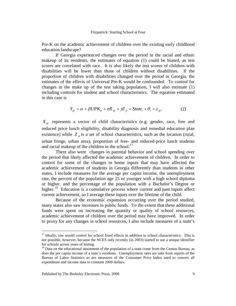
If Georgia experienced changes over the period in the racial and ethnic makeup of its residents, the estimates of equation (1) could be biased, as test scores are correlated with race. It is also likely the test scores of children with disabilities will be lower than those of children without disabilities. If the proportion of children with disabilities changed over the period in Georgia, the estimates of the effects of Universal Pre-K would be confounded. To control for changes in the make up of the test taking population, I will also estimate (1) including controls for student and school characteristics. The equation estimated in this case is

.ijttijtijtitijt StateZXUPKY εθγσβα ++++++= (2)

ijtX represents a vector of child characteristics (e.g. gender, race, free and

reduced price lunch eligibility, disability diagnosis and remedial education plan existence) while jtZ is a set of school characteristics, such as the location (rural,

urban fringe, urban area), proportion of free- and reduced-price lunch students and racial makeup of the children in the school.17 There also were changes in parental behavior and school spending over the period that likely affected the academic achievement of children. In order to control for some of the changes in home inputs that may have affected the academic achievement of students in Georgia differently than students in other states, I include measures for the average per capita income, the unemployment rate, the percent of the population age 25 or younger with a high school diploma or higher, and the percentage of the population with a Bachelor’s Degree or higher.18 Education is a cumulative process where current and past inputs affect current achievement, so I average these inputs over the lifetime of the child. Because of the economic expansion occurring over the period studied, many states also saw increases in public funds. To the extent that these additional funds were spent on increasing the quantity or quality of school resources, academic achievement of children over the period may have improved. In order to proxy for any changes in school resources, I also include measures of a state’s

17 Ideally, one would control for school fixed effects in addition to school characteristics. This is not possible, however, because the NCES only recently (in 2003) started to use a unique identifier for schools across years of testing. 18 Data on the educational attainment of the population of a state come from the Census Bureau, as does the per capita income of a state’s residents. Unemployment rates are take from reports of the Bureau of Labor Statistics as are measures of the Consumer Price Index used to convert all expenditure and income data to constant 2000 dollars.

9



school expenditures per student and the state’s student-to-teacher ratio.19 Again because education is a cumulative process, I average these controls over the period in which the child was likely enrolled (the previous four years).

Additionally, over the period an increasing amount of attention was focused on school accountability, culminating in the passage of the No Child Left Behind legislation of 2002 (NCLB). Accountability and NCLB likely had impacts on children’s test scores, as test scores are exactly what they were designed to improve, but such impacts may have occurred through mechanisms other than expenditures (e.g. through changes in curricula). Though NCLB was national, states began implementing their own accountability systems at different points over the 1990s. I follow Hanushek and Raymond (2005) and define a state as having an accountability system beginning in the year it introduced its own accountability system with consequences for “failing” schools or 2003 (the year in which NCLB required states have their plans in place), whichever came first. I then include controls for both the presence of this type of accountability system and the number of years for which the accountability system has been in place in the state. III.b. Grade Retention If Universal Pre-K does indeed increase school-preparedness, it could be argued that it should affect the number of students being held back. That is, if students are better prepared for kindergarten, they are less likely to repeat kindergarten, potentially less likely to repeat first grade, and so on. Although the NAEP data do not report specifically whether or not a child was held back at any point, information about age and birth month can be used to determine whether or not a child is “on-grade” relative to others his/her age. Specifically, I construct a variable ONGRADE, which takes on a value of one if a child is at or below the median age for his or her state, test year cohort, grade and birth month or a value of zero if the child is above the median age.20 Over the pre-treatment period, between eighty and ninety percent of students were on-grade for their age using this measure (Tables 2 and 3). Because of red-shirting – the name given to the deliberate choice to start a child in school a year after he or she is first eligible made by some parents (rather than by the teacher or school based on a child’s performance) – when ONGRADE is used as the dependent variable, the estimates produced are attenuated. Casico (2005) estimates about one-fifth of “non-repeaters” are old for their class and about one-tenth of repeaters are not. She shows this measurement error leads to estimates 19 These data on school resources come from the Common Core of Data, a product of the National Center for Education Statistics, available at http://nces.ed.gov/ccd/. 20 The same measure is used in other work, for example Oreopolous et al. (2006).

10



that are biased downward by 35 percent when the measure is used as the dependent variable, as it is here. This is due to the fact that many of the children who appear to have repeated a grade actually have not, so decreases in the probability of being on-grade due to grade retention will not seem as large when compared to the whole population of children relatively old for their grade as they would when only repeaters are measured. However, I use it because it is the best available measure in the existing data. The regressions explained in the previous section are estimated using ONGRADE as the dependent variable.21 Because the variable ONGRADE is created in the exact same way for children taking either the reading or math NAEP, I have collapsed the two data sets together. This creates a sample of children with data in seven years (rather than just the four for math or five for reading, see Table 1).

IV. Data IV.a. Overview of the NAEP The data used in this project are the State NAEP in Mathematics and Reading.22 In addition to test scores, administrators of the NAEP collect other information through detailed questionnaires filled out by students, teachers and school administrators. As such, the data include individual-level covariates including gender, race/ethnicity, whether the child has learning needs or limited English proficiency, and whether the child is eligible for a free- or reduced-price school lunch or Title 1 funds. I also include controls at the school level for size, racial make-up of the school, and the percent of students who qualify for free or reduced price lunch or Title 1. Lastly, I include a measure of the location of the school based on Census definitions as to whether the school is located in a central city, urban fringe/large town or rural area/small town.23

21 The results do not change appreciably if the measure of being on-grade for your age is defined at the median prior to the program’s implementation. 22 Begun in 1969, the NAEP is the only ongoing national survey of students’ educational ability and achievement. The NAEP assessments measure the abilities of students ages 9, 13 and 17 in the spring of the year in which they are given. The tests include questions testing students’ knowledge of mathematical concepts such as fractions, use of number patterns, ability to read graphs and reading skills. The State NAEP is designed to have representative samples of the children in each state. For more about the design and implementation of the assessments see Rogers and Stoeckel (2004). 23 From the Census definitions of locations: “A Central City is a city of 50,000 people or more that is the largest in its metropolitan area, or can otherwise be regarded as “central,” taking into account such characteristics as commuting patterns. Urban Fringe includes all densely settled places and areas within MSAs that are classified as urban by the U.S. Census Bureau. A Large Town is defined as a place outside MSAs with a population greater than or equal to 25,000. Rural

11



In order to encourage full participation by students, the NAEP uses a system of testing called the “Balanced Incomplete Block Spiral Method”. This method essentially offers only a partial set of the complete test to each student being assessed. In effect, each student is only required to take an hour-long test, but the result is that students’ tests are not accurate measures of their knowledge and are not comparable across the population. To address this problem, the NAEP calculates each student’s “plausible values”, which are drawn from a distribution of test scores for students with the same observable characteristics and pattern of correct responses to answered questions. Because of these scaling techniques, students’ total raw test scores are biased estimates of their ability. I therefore use plausible scores as the dependent variable.24 IV.b. Take-Up and Enrollment in Preschool The issues of take-up and crowd-out are fundamental to my research question. As a consequence, there are likely differential treatment effects for different subgroups of the total population to whom Universal Pre-K was offered. One reason is different groups had different options available to them before the advent of Universal Pre-K. For example, rural areas may have offered fewer child care options because there are fewer children (or perhaps reduced demand for child care). Secondly, families who differ by income have different resources available to them. Many high-income families were likely sending their children to high-quality preschool or day care even before Universal Pre-K was introduced. When the program began, these families may simply get for free what they were paying for themselves. Lastly, there may be different labor supply effects of this subsidy, which in turn may affect educational outcomes. Some parents may be induced to work as a result of subsidy receipt, while others may not. All of these are reasons why the effects of the program may differ across various socioeconomic characteristics of the families.25 One result of the program’s introduction might be that general preschool enrollment increases because families not previously enrolling their children in preschool are now sending their child to Pre-K. If take-up of the subsidy by those

includes all places and areas with a population of less than 2,500 that are classified as rural by the Bureau of Census. A Small Town is defined as a place outside MSAs with a population of less than 25,000 but greater than or equal to 2,500” Rogers and Stoeckel (2004). 24 A full explanation of plausible values can be found in Rogers and Stoeckel (2004) and Horkay (1999). Most researchers use the plausible value scores when conducting analyses using the NAEP. For examples, see Grissmer and Flanagan (2001), Miller and Zhang (2007). Although he does not use the plausible values, Jacob (2007) also includes a discussion of their necessity. 25 An analysis of the labor supply effects of these child care subsidies is beyond the scope of the current paper but is included in Fitzpatrick (2008).

12



who were not sending their children to preschool were the only effect of the program, one would expect to see Pre-K enrollment and overall preschool enrollment (which includes Pre-K enrollment) increase. However, some families are willing to pay to send their children to preschool in the absence of Universal Pre-K. When the state offers to pay for their children to attend Pre-K, these families might just switch the enrollment of their children from regular preschool to classrooms which are part of the Pre-K system. 26 If this type of crowding-out occurs, Pre-K (government-sponsored preschool) enrollment will increase, but overall preschool enrollment may not. Figure 2 presents descriptive information about patterns of preschool enrollment of four-year olds in all other states and in Georgia, taken from the October Supplement to the Current Population Surveys (CPS), 1991-2001.27 Because the sample sizes are small, estimates using CPS data for one age in one state are particularly noisy. It is apparent that there is a national trend of increasing enrollment in preschool over the period. In states not enacting Universal Pre-K, enrollment rates rose from 53 to 66 percent of the population of four year olds. In Georgia, the increase in preschool attendance by four year olds is steeper than in other states. In years after Universal Pre-K introduction (FY96 to FY02) enrollment is higher than in the “baseline” year, FY92, in which enrollment is only at 40 percent. One program very much related to Pre-K is Head Start. The federal Head Start program provides early childhood education (and other services) to children whose families have income below poverty level. Such programs often run the entire year and provide more hours of care than Universal Pre-K. Because Head Start targets some of the same population studied in this analysis and the empirical strategy assumes there were no concurrent policy or behavioral shifts particular to this population of students in Georgia that might have affected test scores and grade retention, I check that there were no major changes in Head Start enrollment in this population at the time of the introduction of Universal Pre-K in Georgia. Figure 3 shows the enrollment of children in Georgia (as a percentage of all four year olds) in Head Start from FY92 to FY02. Over the period, the percentage enrolled increased from 9.8 to 10.4 percent. The change appears to be unrelated to the timing of Universal Pre-K in Georgia. The figure also shows that the entire U.S. saw similar patterns in Head Start enrollment rates over the period.

26 Another dimension along which enrollment behavior may change is that families might decide to increase or decrease the number of hours of care being purchased. 27 The question asked of parents is whether their child is attending “nursery school or kindergarten”.

13



Figure 2: Percent of Four Year Olds Enrolled in Any Type of Preschool

0

0.1

0.2

0.3

0.4

0.5

0.6

0.7

0.8

0.9

1

1991

1992

1993

1994

1995

1996

1997

1998

1999

2000

2001

Year

Pe

rcen

t Enr

ollm

ent

Other States Lower Bound Other States Mean Other States Upper Bound

Georgia Lower Bound Georgia Mean Georgia Upper Bound

Georgia program means-tested

Georgia program becomes universal

Note: Numbers based on the author’s calculations using the October Supplement to the Current Population Surveys, 1991-2001. Small sample sizes lead to a large amount of variation in preschool enrollment rates in Georgia. Dotted lines represent the 90 percent confidence intervals.

14



Figure 3. Percent of Four Year Olds Enrolled in Head Start Programs

9.8%

11.1% 11.1%10.6% 10.7% 10.9% 11.0% 10.9%

10.1%10.8% 10.4%

10.4%

11.8% 11.8%11.3% 11.6%

12.1%12.4% 12.7%

11.4%12.0% 11.6%

0%

5%

10%

15%

FY92

FY93

FY94

FY95

FY96

FY97

FY98

FY99

FY00

FY01

FY02

Georgia U.S.

Notes: Head Start enrollment information found in the Digest of Education Statistics, 1995 to 2005 A fiscal year runs from October of the previous year to September of the year in its name. For example, FY96 runs from October 1, 1995 to September 30, 1996. Reported Head Start enrollment can include children of all ages, but in each year the number of Head Start enrollees is multiplied by the fraction of enrollees in Head Start across the nation who are four years old. Percent of population of four year olds is calculated using the Census Bureau’s Time Series of State Population Estimates by Age.

15



IV.c. Descriptive Statistics Tables 2 and 3 show characteristics of the children by year of testing for Georgia and the other states, respectively.28 Georgia has both more African-American students than the rest of the U.S. (45 versus 16 percent) and more children in fourth grade who are eligible for the National School Lunch Program (NSLP), (50 versus 39 percent). Georgia has a slightly smaller proportion of its fourth graders living in central cities and a slightly larger proportion in areas designated as urban fringe than the rest of the country. Fourth graders in Georgia are slightly less likely to have a remedial Education Plan, either Language or Individualized. Table 2: Descriptive Statistics of Students in Georgia

1994 1996 1998 2000 2002 2003 2005 Standardized Math Score

-0.045 -0.011 0.084 0.101 (0.268) (0.264) (0.005) (0.005)

Standardized Reading Score

-0.033 -0.013 0.029 0.027 0.018 (0.388) (0.342) (0.326) (0.006) (0.007)

On-grade 0.796 0.828 0.858 0.882 0.834 0.823 0.840 (0.403) (0.378) (0.349) (0.323) (0.372) (0.382) (0.367) Female 0.524 0.498 0.502 0.528 0.484 0.486 0.499 (0.500) (0.500) (0.500) (0.499) (0.500) (0.500) (0.500) White 0.626 0.603 0.544 0.518 0.547 0.532 0.444 (0.484) (0.489) (0.498) (0.500) (0.498) (0.499) (0.497) Black 0.334 0.343 0.403 0.420 0.367 0.483 0.347 (0.472) (0.475) (0.491) (0.494) (0.482) (0.369) (0.476) Education Plan 0.056 0.065 0.039 0.090 0.122 0.122 (0.229) (0.246) (0.194) (0.286) (0.327) (0.327) NSLP Eligible 0.355 0.411 0.475 0.420 0.440 0.445 0.525 (0.479) (0.492) (0.499) (0.494) (0.496) (0.497) (0.499) Disability 0.041 0.051 0.032 0.002 0.045 0.084 0.088 (0.198) (0.220) (0.176) (0.040) (0.208) (0.278) (0.283)

Note: Based on the author’s calculations using the National Assessment of Educational Progress. To correctly account for the design of the survey, weights and jackknife procedures for calculating sample variance were used. Standard deviations are in parentheses. Test scores have been standardized to have mean zero and standard deviation of one in 1996 for math and 1994 for reading. Survey population weights were used.

28 School characteristics can be found in Appendix Tables 1 and 2.

16



Table 3: Descriptive Statistics of Students in the Rest of the U.S. (Not Georgia)

1994 1996 1998 2000 2002 2003 2005 Standardized Math Score

0.002 0.057 0.116 0.142 (0.272) (0.249) (0.001) (0.001)

Standardized Reading Score

0.001 0.025 0.056 0.054 0.061 (0.357) (0.333) (0.320) (0.002) (0.002)

On-grade 0.825 0.853 0.878 0.875 0.852 0.838 0.840 (0.380) (0.354) (0.327) (0.331) (0.355) (0.368) (0.367) Female 0.499 0.492 0.505 0.512 0.494 0.492 0.495 (0.500) (0.500) (0.500) (0.500) (0.500) (0.500) (0.500) White 0.683 0.670 0.653 0.650 0.613 0.603 0.533 (0.465) (0.470) (0.476) (0.477) (0.487) (0.489) (0.499) Black 0.153 0.152 0.164 0.179 0.161 0.159 0.139 (0.360) (0.359) (0.370) (0.383) (0.368) (0.366) (0.346) Education Plan 0.096 0.095 0.091 0.137 0.167 0.176 (0.295) (0.294) (0.288) (0.344) (0.373) (0.381) NSLP Eligible 0.339 0.366 0.377 0.375 0.394 0.401 0.414 (0.473) (0.482) (0.485) (0.484) (0.489) (0.490) (0.493) Disability 0.050 0.049 0.045 0.001 0.061 0.082 0.088 (0.218) (0.216) (0.208) (0.026) (0.239) (0.274) (0.283)


V. Results V.a. Average Statewide Effects A visual inspection over the period suggests Universal Pre-K had a positive effect on the average math and reading scores of fourth graders in Georgia. Figure 4 plots the average standardized fourth grade math (Panel A) and reading (Panel B) scores over the period studied.29 The vertical line in each figure represents the last cohort to not have had access to Universal Pre-K. Average test scores in both Georgia and the rest of the U.S. rise over the period, though the average math and reading scores of Georgia are lower than those in the rest of the U.S. For example, the average standardized math score for the students in Georgia in 1996 was 0.05 standard deviations lower than the average standardized score for the rest of the U.S. The narrowing of the distance between the average scores in

29 Only tested cohorts for each subject are in the figures.

17



Figure 4. Standardized 4th Grade NAEP Scores, Georgia vs. Rest of the U.S. (Line indicates last pre-program cohort) Panel A. Mathematics Scores

-0.1

-0.05

0

0.05

0.1

0.15

0.2

1996 2000 2003 2005

Year

Sta

nd

ard

ized

Sco

re

GeorgiaOther States

Panel B. Reading Scores

-0.04

-0.02

0

0.02

0.04

0.06

0.08

1994 1998 2002 2003 2005

Year

Sta

nd

ard

ized

Sco

re

Other StatesGeorgia

Note: Based on the author’s calculations from the State NAEP Restricted Use files. Test scores have been standardized to have mean zero and standard deviation of one in 1996 for math and 1994 for reading. Survey population weights were used.

18



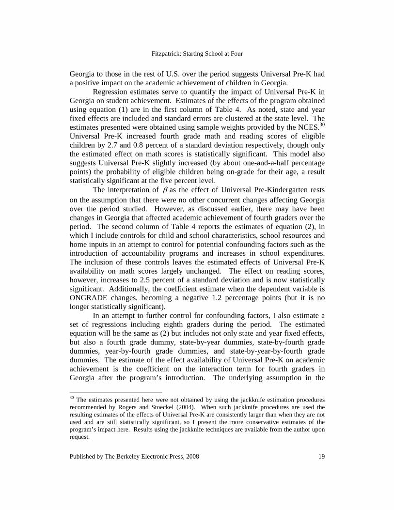
Georgia to those in the rest of U.S. over the period suggests Universal Pre-K had a positive impact on the academic achievement of children in Georgia. Regression estimates serve to quantify the impact of Universal Pre-K in Georgia on student achievement. Estimates of the effects of the program obtained using equation (1) are in the first column of Table 4. As noted, state and year fixed effects are included and standard errors are clustered at the state level. The estimates presented were obtained using sample weights provided by the NCES.30 Universal Pre-K increased fourth grade math and reading scores of eligible children by 2.7 and 0.8 percent of a standard deviation respectively, though only the estimated effect on math scores is statistically significant. This model also suggests Universal Pre-K slightly increased (by about one-and-a-half percentage points) the probability of eligible children being on-grade for their age, a result statistically significant at the five percent level. The interpretation of β as the effect of Universal Pre-Kindergarten rests on the assumption that there were no other concurrent changes affecting Georgia over the period studied. However, as discussed earlier, there may have been changes in Georgia that affected academic achievement of fourth graders over the period. The second column of Table 4 reports the estimates of equation (2), in which I include controls for child and school characteristics, school resources and home inputs in an attempt to control for potential confounding factors such as the introduction of accountability programs and increases in school expenditures. The inclusion of these controls leaves the estimated effects of Universal Pre-K availability on math scores largely unchanged. The effect on reading scores, however, increases to 2.5 percent of a standard deviation and is now statistically significant. Additionally, the coefficient estimate when the dependent variable is ONGRADE changes, becoming a negative 1.2 percentage points (but it is no longer statistically significant). In an attempt to further control for confounding factors, I also estimate a set of regressions including eighth graders during the period. The estimated equation will be the same as (2) but includes not only state and year fixed effects, but also a fourth grade dummy, state-by-year dummies, state-by-fourth grade dummies, year-by-fourth grade dummies, and state-by-year-by-fourth grade dummies. The estimate of the effect availability of Universal Pre-K on academic achievement is the coefficient on the interaction term for fourth graders in Georgia after the program’s introduction. The underlying assumption in the

30 The estimates presented here were not obtained by using the jackknife estimation procedures recommended by Rogers and Stoeckel (2004). When such jackknife procedures are used the resulting estimates of the effects of Universal Pre-K are consistently larger than when they are not used and are still statistically significant, so I present the more conservative estimates of the program’s impact here. Results using the jackknife techniques are available from the author upon request.

19



Table 4: Difference-in-Differences Estimates of the Effect of Universal Pre-K in Georgia on Test Scores and Probability of Being On-Grade (I) (II) (III) (IV) (V) (VI) (VII) Math Score 0.027 0.025 0.017 (-0.007, 0.092) 0.013 0.011 0.008 (0.006) (0.007) (0.006) {0.111} (0.008) (0.006) Reading Score 0.008 0.025 0.024 (-0.005,0.077) 0.009 0.017 0.013 (0.007) (0.002) (0.020) {0.350} (0.016) (0.012) On-grade 0.015 -0.012 -0.005 (-0.035, 0.036) 0.008 0.006 0.007 (0.006) (0.007) (0.005) {0.026} (0.007) (0.007) Specification Details Observation Level Student Student Student State Student Student Grades Included 4 4 4 & 8 4 4 4 & 8 Controls Included N Y Y Y Y Y Clustering State State State n/a State State Weighting Survey Survey Survey Synthetic Synthetic Synthetic Number of Observations Math Score 537,112 537,112 1,013,847 537,112 27 406,914 773,734 Reading Score 714,894 714,894 1,397,312 714,894 20 156,941 269,860 On-grade 1,241,994 1,241,994 2,468,988 1,241,994 29 111,422 218,836

Note: Based on the author’s calculations using the NAEP. All regressions include state and year fixed effects as well as controls for student and school characteristics. Survey weights were used. See Rogers and Stoeckel (2004) for more information. The dependent variables in the first two sets of rows are an individual child’s plausible test score on the Mathematics and Reading Assessments, respectively. The scores have been standardized by the mean and standard deviation of the first year of data for that subject. The dependent variable in the third set of rows is a dummy variable for whether the child was at or above the median age for his/her state, grade and cohort. The estimates in the third row are from linear probability models using all years of Mathematics and Reading data. Standard errors are in parentheses. Estimates allow for arbitrary correlation of the error terms at the state level. The fourth column gives the 90% confidence interval range using the methods detailed in Conley and Taber (2006). The last three columns report results using the synthetic control methods from Abadie et al. (2007) as detailed in the text. In the fifth column, the {} contain probability values of the estimate being within the 95 percent confidence interval.

20



interpretation of this as the effect of Universal Pre-K availability in this D-D-D model is that other changes over the period affected the academic achievement of fourth and eighth graders in Georgia similarly. The results of this estimation are in column III of Table 4.31 The inclusion of eighth graders in the control group changes the estimated effect of Universal Pre-K availability on math scores, reading scores and the probability of being on-grade to an increase of 1.7 percent of a standard deviation, an increase of 2.4 percent of a standard deviation and a decrease of 0.5 percentage points, respectively. Only the estimated effect on math test scores is statistically significant. There has been much discourse in the literature about inference in D-D methods, including discussion of the asymptotic distribution of the estimate. One issue is whether there exist enough actual treatment and/or control groups in the data to assume standard asymptotics (whereby the observations are independent and the number of periods, treatment and control groups approaches infinity – see Moutlon 1990, Donald and Lang 2007). A recent example is Conley and Taber (2006), in which the authors present an alternative approach to calculating confidence intervals when there are a small number of treatment groups (such as here, where it is arguable there is only one).32 Using this method results in wider confidence intervals than either of the others discussed (column VI of Table 4). Even so, the bulk of the intervals for the math and reading scores analyses lie in the positive range.33 It may not be reasonable to assume the most appropriate control group for Georgia is the entire set of other states. Specifically, one might think Georgia has more in common, especially educationally and economically, with its neighbors (such as Alabama and Louisiana) than it does with states located far away and/or that have very different characteristics (such as California and Alaska). Additionally, Figure 5 suggests that the trend in test performance of fourth graders may have different in Georgia than it was in other states.34 31 Note that eighth graders in Georgia taking the NAEP tests in the spring of 2005 also would have been exposed to Universal Pre-K in its first year. Because there is only one year of data for treated eighth graders and the program was not fully implemented in its first year (see Figure 1), I include an interaction term for the effect of Universal Pre-Kindergarten on eighth graders but do not present or interpret its results. Results are available from the author upon request. 32 Essentially, the Conley and Taber method involves using asymptotic approximations that let the control group grow large while holding the number of observations in the treatment group fixed. Inference about the effect of treatment is then made by in a sense comparing the outcome for the treatment group to the distribution of the outcome for the control group. 33 Only 7 and 6 percent of the estimated confidence interval for the effect of Universal Pre-K on math and reading scores, respectively, lies below zero. 34 For example, results of a placebo D-D test placing treatment in 1998 estimates math scores decreased by 1.7 percent of a standard deviation from 1996 to 2000 (relative to scores in other states).

21



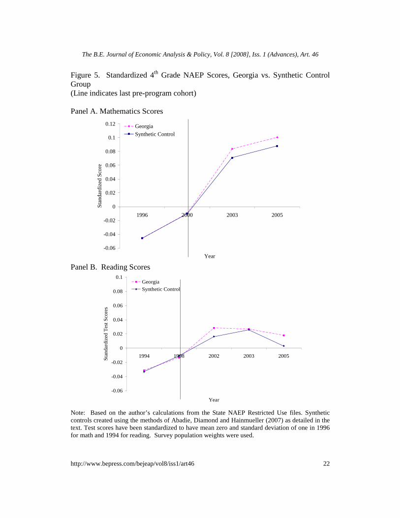
Figure 5. Standardized 4th Grade NAEP Scores, Georgia vs. Synthetic Control Group (Line indicates last pre-program cohort) Panel A. Mathematics Scores

-0.06

-0.04

-0.02

0

0.02

0.04

0.06

0.08

0.1

0.12

1996 2000 2003 2005

Year

Sta

ndar

dize

d S

core

Georgia

Synthetic Control


-0.06

-0.04

-0.02

0

0.02

0.04

0.06

0.08

0.1

1994 1998 2002 2003 2005

Year

Sta

nda

rdiz

ed T

est

Sco

res

GeorgiaSynthetic Control

Note: Based on the author’s calculations from the State NAEP Restricted Use files. Synthetic controls created using the methods of Abadie, Diamond and Hainmueller (2007) as detailed in the text. Test scores have been standardized to have mean zero and standard deviation of one in 1996 for math and 1994 for reading. Survey population weights were used.

22



Abadie et al. (2007) outline a data-driven approach for constructing an appropriate synthetic control group (and making inferences) in “case-studies” such as this one. In the current context, their method involves creating a synthetic control group using a combination of other states that best mimics the observable characteristics and pre-treatment outcomes of Georgia fourth graders.35 Of particular benefit for this context, the use of the Abadie et al. (2007) method relaxes the D-D assumption that unobserved confounding factors be constant over time by allowing them to vary over the period in question. Panel A of Figure 5 contains a plot of the standardized math test scores of Georgia and a synthetic control group I created using the weighted combination of states that best reproduced the pre-treatment math scores of Georgia.36 Panel B does the same for a synthetic control created to match pre-treatment reading scores. As evident in the figure, this method does an excellent job of creating synthetic control groups that match the pre-treatment trends in test scores in Georgia.37 Further, both figures suggest Georgia test scores increased relative to those of the synthetic control group with the introduction of Universal Pre-K. The difference in test scores for Georgia and its synthetic control was 1.3 percent of a standard deviation and 0.009 percent of a standard deviation for math and reading, respectively (Column VII of Table 4). To make statistical inference about these increases, Abadie et al. (2007) suggest conducting placebo tests which involve creating synthetic control groups for the other states in the sample. One can then compare the size of the “post-treatment” gap in test scores for Georgia and its synthetic control to the gap for other states that did not introduce Universal Pre-K. If the gap in scores is in fact due to the introduction of Universal Pre-K rather than other confounding factors, there should be no gap between the test scores of non-treated states and their synthetic controls. Figure 6 plots these gaps in test scores using only placebo tests whose mean squared prediction error was less than a thousand times that of Georgia’s synthetic control. Three of the twenty-seven placebo tests had gaps as large as or larger than Georgia’s in math scores. The probability of estimating a gap the size of Georgia’s from a random assignment of the intervention in the data is 3/27, or 0.111; for reading this probability is 0.350. Neither of these estimates

35 In practice this involves creating a vector of weights which sum to one and minimize the distance between the observable characteristics and pre-treatment outcomes of the treatment group and the synthetic control group. In other words, I choose the combination of other states that best mimics the test scores (or percent of students on-grade for their age) of Georgia prior to the introduction of Universal Pre-K. 36 The weights are presented in Appendix Table 3. 37 The mean squared prediction errors (MSPE) for the synthetic control groups are much smaller than zero (e.g. for math the MSPE is 0.0000375, whereas the MSPE in Abadie, Diamond and Hainmueller [2007] are on the order of 3). MSPEs for each synthetic control group are available from the author upon request.

23



Figure 6. Gaps in Standardized 4th Grade NAEP Scores for Georgia and Placebo Treatment States (Line indicates last pre-program cohort) Panel A. Mathematics Scores

-0.1

-0.08

-0.06

-0.04

-0.02

0

0.02

0.04

0.06

0.08

0.1

1996 2000 2003 2005

Year

Gap

in S

tan

dard

ized

Sco

re


-0.06

-0.04

-0.02

0

0.02

0.04

0.06

0.08

0.1

1994 1998 2002 2003 2005

Year

Ga

p in

Sta

ndar

dize

d T

est

Sco

res

Note: Based on the author’s calculations from the State NAEP Restricted Use files. The pink lines represent the test score gap between Georgia and its synthetic control using the methods of Abadie, Diamond and Hainmueller (2007). Grey lines represent the gaps for the placebo groups. See text for details. Test scores have been standardized to have mean zero and standard deviation of one in 1996 for math and 1994 for reading. Survey population weights were used.

24



is statistically significant at conventional levels. The process was repeated using the probability of being on-grade for one’s age as the outcome. Here the estimated effect of Universal Pre-Kindergarten introduction is 0.008, which is also not statistically significant. To apply the synthetic control group method to individual data, I multiplied the sample weights for each student’s observation by the corresponding weight for the student’s state of residence from the synthetic control method. Results of the D-D and D-D-D estimation using these weights and the micro-data are in the sixth and seventh columns of Table 4.38 The estimated effects of Universal Pre-K availability on test scores and grade retention are positive, but are not statistically significant, suggesting there were no discernable effects on statewide academic achievement. In summary, estimates of the statewide effects of Universal Pre-K in Georgia generally indicate that the program's availability improved child outcomes by as much as one to three percent of a standard deviation but the use of appropriate control groups and methods of inference renders the estimated relationship statistically insignificant. Because of the strengths of the synthetic control group method, in what follows I replicate this procedure, obtaining state weights for synthetic control groups that best match the pre-treatment outcome of interest for the group specified and multiplying these state weights by the NCES sample weights for each observation. V.b. Heterogeneous Effects Potentially different effects of Universal Pre-K on different subgroups of the population may result from differential opportunities available to children and families prior to the introduction of the program. For example, the population density of young children in cities is ten times as high as that in rural areas (50 children per square mile versus 5). Lack of other young children likely means fewer child care providers. Meanwhile, only 36 percent of women over the age of 16 in rural areas are employed, while in cities over 50 percent are. In order to examine whether the effects of Universal Pre-K availability differ for different subgroups of the population, Table 5 presents estimates of the effects of Universal Pre-K availability separately for various subgroups of the total population of fourth graders: Caucasian students ineligible for NSLP, African-American students ineligible for NSLP, Caucasian students eligible for NSLP and African-American students eligible for NSLP in columns I through IV, respectively.

38 As a final check, I also estimated the effects of Universal Pre-K using these weights and allowing for state specific trends in test scores over the period. The results are similar to those here in that the estimates of the effects of Universal Pre-K are positive, but not statistically distinguishable from zero.

25



Table 5. Difference-in-Differences Estimates of the Effect of Universal Pre-K on Students’ Test Scores and Probability of Being On-Grade of Students by Race and School Lunch Eligibility Status

(I) (II) (III) (IV) Race White Black White Black School Lunch Eligible No No Yes Yes Math Score 0.036 -0.009 0.082 0.000 (0.007) (0.015) (0.008) (0.011) 96,148 17,670 7,738 47,916 Reading Score -0.009 0.018 -0.024 -0.013 (0.007) (0.015) (0.025) (0.019) 204,767 26,979 89,092 67,314 On-grade -0.001 0.060 0.020 0.025 (0.005) (0.022) (0.004) (0.010) 370,227 50,342 22,462 107,371

Note: Based on the author’s calculations using the National Assessment of Educational Progress. Column headers indicate the subgroups of the population included in the sample. The first row of each set represents the coefficient estimates, the second row (in parentheses) reports the standard error of the estimate above it and the third row reports the number of observations used in estimation. Test scores have been normalized by the average standard deviation for all plausible values in the first year of data for that test. All regressions include year and state fixed effects. Controls for student and school characteristics included are described in the text. To correctly account for the design of the survey, weights were used (Rogers and Stoeckel 2004). Estimates allow for arbitrary correlation of the error terms at the state level. Synthetic control groups were created using the Abdaie, Diamond and Hainmueller (2007) method as detailed in the text. Estimates in bold are significant at the five percent level or lower. The results in Table 5 show that the math scores of some children improved because of the introduction of Universal Pre-K in Georgia. The math scores of Caucasian children ineligible for NSLP increased by 3.6 percent of a standard deviation. Similarly, the math scores of NSLP-eligible Caucasian children increased by 8.2 percentage points. However, the estimates of the program’s introduction on the math scores of African-American children and on the reading scores of any of these groups are not statistically different from zero. With the exception of Caucasian NSLP-ineligible children, the introduction of Universal Pre-K produced increases in the probability of fourth graders in Georgia being on-grade for their age. African-Americans who were

26



ineligible for NSLP were 6 percentage points and NSLP children (both African-American and Caucasian) were about 2 percentage points more likely to be on-grade for their age because of the availability of Universal Pre-K. These increases are not trivial given that about 80 percent of children are on-grade for their age in Georgia before the program. Since these decreases in the proxy for grade retention are not always accompanied by increases in test scores, it is plausible the program has effects on skills not measured by test scores. There is much discussion among researchers about the developmental differences between boys and girls, with some research showing early childhood interventions may have larger impact on girls than on boys. For example, analysis by Anderson (2005) argues the benefits of Perry Preschool Project, Abecedarian and Early Training Projects were accrued by the female participants. On average, the math scores of male fourth graders in my sample are 0.03 standard deviations higher than those of females, ceteris paribus. However, there is no differential effect of Universal Pre-K by gender for any of the subgroups discussed above.39 Fitzpatrick (2008) examines the changes in preschool enrollment behavior of families in response to Universal Pre-K availability. She finds mothers whose have at most enrolled in college without receiving a degree are more likely to enroll their children in preschool because of Universal Pre-K than they would be in the program’s absence. Additionally, she finds women in rural and urban fringe (small town) areas are the group induced to make the largest changes in their enrollment of their four year olds in preschool because of Universal Pre-K. To see how these changes in enrollment patterns translate into changes into children’s achievement, I examine the effects of Universal Pre-K by race, NSLP eligibility and residential area. The results are presented in Table 6; in the table, the estimates across the columns represent the groups as they did in Table 5, by race and NSLP-eligibility status, while the blocks of rows report different coefficients by area of residence. When interpreting the results presented in Table 6, it is important to keep in mind that the three residential categories do not correlate to cities, suburbs and small towns. Rather, cities and suburbs tend to be included together in the “urban area” category.40 The results in Table 6 suggest that disadvantaged Caucasian children in rural and urban fringe areas are those most likely to gain from Universal Pre-K availability. The math scores of these children increase by 6 to 9 percent of a standard deviation. Their reading scores increase by 3 to 7 percent of a standard deviation and they are at least 2 percentage points more likely to be on-grade for their age. Though the effects are not as consistently statistically significant, there

39 Results are omitted in the interest of brevity, but are available from the author upon request. 40 A map showing the precise division of areas into the three categories can be found in Fitzpatrick (2008).

27



Table 6. Difference-in-Differences Estimates of the Effect of Universal Pre-K on Students’ Test Scores and Probability of Being Ongrade of Students by Race, School Lunch Eligibility Status and Area of Residence

(I) (II) (III) (IV) Race White Black White Black School Lunch Eligible No No Yes Yes

Urban Area Math Score 0.024 0.000 0.018 0.008 (0.009) (0.011) (0.013) (0.013) 38,002 8,069 13,983 26,187 Reading Score 0.020 0.087 -0.024 -0.009 (0.027) (0.037) (0.022) (0.026) 52,614 12,132 18,054 35,542 On-grade -0.009 0.068 -0.046 0.074 (0.029) (0.023) (0.038) (0.025) 9,437 3,513 3,281 12,619

Urban Fringe Math Score 0.036 0.006 0.091 -0.013 (0.007) (0.023) (0.002) (0.015) 96,148 12,846 7,738 16,699 Reading Score 0.001 0.017 0.028 -0.002 (0.007) (0.033) (0.013) (0.017) 99,256 9,496 25,245 14,325 On-grade 0.004 0.039 0.017 0.072 0.005 0.025 0.004 0.023 150,032 2,319 36,204 7,463

Rural Math Score 0.093 0.048 0.064 0.001 (0.017) (0.019) (0.014) (0.017) 65,504 3,294 27,068 12,297 Reading Score 0.014 -0.042 0.072 0.121 (0.013) (0.060) (0.034) (0.017) 92,837 5,124 44,478 2,901 On-grade 0.007 0.031 0.044 0.053 0.006 0.002 0.012 0.002 142,904 3,761 10,661 49,641

Note: Based on the author’s calculations using the NAEP. The first row of each set represents the coefficient estimates, the second row (in parentheses) reports the standard error of the estimate above it and the third row reports the number of observations used in estimation. Test scores have been normalized by the average standard deviation for all plausible values in the first year of data for that test. All regressions include year and state fixed effects. Controls for student and school characteristics are included are described in the text. Survey weights were used (Rogers and Stoeckel 2004). Estimates allow for arbitrary correlation of the error terms at the state level. Synthetic control groups were created using the Abdaie at al. (2007) method as detailed in the text. Estimates in bold are significant at the five percent level or lower.

28



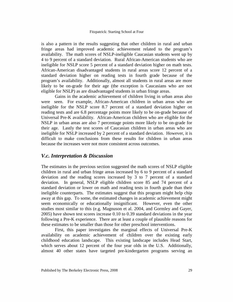
is also a pattern in the results suggesting that other children in rural and urban fringe areas had improved academic achievement related to the program’s availability. The math scores of NSLP-ineligible Caucasian students went up by 4 to 9 percent of a standard deviation. Rural African-American students who are ineligible for NSLP score 5 percent of a standard deviation higher on math tests. African-American disadvantaged students in rural areas score 12 percent of a standard deviation higher on reading tests in fourth grade because of the program’s availability. Additionally, almost all students in rural areas are more likely to be on-grade for their age (the exception is Caucasians who are not eligible for NSLP) as are disadvantaged students in urban fringe areas. Gains in the academic achievement of children living in urban areas also were seen. For example, African-American children in urban areas who are ineligible for the NSLP score 8.7 percent of a standard deviation higher on reading tests and are 6.8 percentage points more likely to be on-grade because of Universal Pre-K availability. African-American children who are eligible for the NSLP in urban areas are also 7 percentage points more likely to be on-grade for their age. Lastly the test scores of Caucasian children in urban areas who are ineligible for NSLP increased by 2 percent of a standard deviation. However, it is difficult to make conclusions from these results for children in urban areas because the increases were not more consistent across outcomes. V.c. Interpretation & Discussion

The estimates in the previous section suggested the math scores of NSLP eligible children in rural and urban fringe areas increased by 6 to 9 percent of a standard deviation and the reading scores increased by 3 to 7 percent of a standard deviation. In general, NSLP eligible children score 85 and 74 percent of a standard deviation or lower on math and reading tests in fourth grade than their ineligible counterparts. The estimates suggest that this program might help chip away at this gap. To some, the estimated changes in academic achievement might seem economically or educationally insignificant. However, even the other studies most similar to this (e.g. Magnuson et al. 2004, and Gormley and Gayer, 2005) have shown test scores increase 0.10 to 0.39 standard deviations in the year following a Pre-K experience. There are at least a couple of plausible reasons for these estimates to be smaller than those for other preschool interventions.

First, this paper investigates the marginal effects of Universal Pre-K availability on academic achievement of children over the existing early childhood education landscape. This existing landscape includes Head Start, which serves about 12 percent of the four year olds in the U.S. Additionally, almost 40 other states have targeted pre-kindergarten programs serving an

29



additional 15 percent of four year olds in 2001-2002.41 The enrollment rates in Figure 2 therefore suggest an additional 15 to 35 percent of four year olds in Georgia were in non-subsidized preschool programs before the introduction of Universal Pre-K. With so many in the control group participating in some form of preschool, it is unlikely that we would see gains as large as would be expected with large shifts on the extensive margin of participation. That the effects are the most pronounced and consistent in areas seeing the largest preschool participation increases is suggestive that changes on the extensive margin have greater impact than increases on the intensive quality margin.

Second, the aforementioned research examined the effects of participation in Pre-K. Estimates presented here are intent-to-treat effects, not estimates of the impact of participation in Universal Pre-K programs. Fitzpatrick (2008) shows Universal Pre-K availability increased enrollment in preschool of children livening in urban fringe areas by 14 percentage points and in rural areas by 12 percentage points. If we assume the only effect of treatment is to induce brand new enrollment in preschool, we can calculate a Wald estimate for the effect of the treatment on the treated that ranges from about one-eighth to one-half of a standard deviation in urban fringe and rural areas. On the other hand, if we assume that the treatment is enrollment in GPK and that enrollment rates of four year olds in different residential areas are similar to the statewide average, the Wald estimate of the treatment-on-the-treated effect on test scores is between 5 and 17 percent of a standard deviation. There were quality mandates involved with the Universal Pre-K program, so it is plausible that the quality of preschool experience improved for many children who would have been enrolled even if Universal Pre-K did not exist. These treatment on the treated estimates are much more in line with the literature on early childhood interventions. Before concluding, it is of interest to consider a cost-benefit analysis of the state’s investment in Universal Pre-K. Such a calculation is difficult because the long-term impacts of the program on wages are not yet known. However, a simple back-of-the-envelope calculation can be done by extrapolating from the combination of estimates of the program’s effects on test scores from this analysis with estimates from other research linking increases in test scores to increases in wages. Murnane et al. (1995) estimate that a standard deviation increase in math scores of high school graduates in 1980 led to increases in wages of between $0.99 and $1.28 (when translated to 2007 dollars). Assuming high school math scores of students in Georgia maintain the same increases seen for fourth graders and the wage differential estimated for 1980 holds for the students in Georgia in the past decade, this implies an increase in wages of less than $0.11 (0.09*$1.28) for each student whose scores increase. I generously assume this group consists

41 http://nieer.org/yearbook2003/pdf/yearbook.pdf#page=18.

30



of 40 percent of a cohort (including most of those in rural areas and some in urban fringe areas). I further assume this increase in wages continues for 50 years (until the cohort retires) and the discount rate is 0.03. If the future income of exposed students is taxed at a rate of 30 percent, the value today of the future gains in tax revenue would be about $56 million. 42 The costs of the program today ($302 million in 2007-2008) greatly outweigh the benefits in terms of potential increased taxable revenue. This is a very simple cost benefit analysis and should therefore be interpreted with caution. However, it is at least suggestive that the government’s scare resources would be better spent on more targeted early childhood interventions that have been shown to be more cost efficient, particularly if the goal is to increase wages through test scores.43

VI. Conclusions

Estimates presented show Universal Pre-K in Georgia led to lasting benefits on the academic achievement of children. Most notably, Universal Pre-K availability increased the test scores of disadvantaged (school-lunch-eligible) children living in areas with relatively low levels of population density by as much as12 percent of a standard deviation. Since the group of disadvantaged children in rural or urban fringe areas makes up about 19 percent of the student population in Georgia, these results are non-trivial. The probability of being on-grade for their age of these children also increased by as much as 7 percentage points. The findings that Universal Pre-K availability increased the academic achievement of children in urban fringe and rural areas corresponds with other research showing that these areas see the largest increases in preschool enrollment because of the program’s availability.

Statistically significant gains for other groups of children are also seen on some of the measures of academic achievement but not all, which leads me to be cautious in making any conclusions about the effects of the program for these groups. These first estimates of the longer-term effects of Universal Pre-K support the findings in the literature that gains from Universal Pre-K programs are not universal, but are “targeted” within certain groups. The results of the study and its cost benefit analysis indicate scarce public funds may be used more efficiently by implementing targeted strategies in the design of Pre-K programs,

42 There were approximately 120,000 four year olds in Georgia in 2005. I assume each works 2,000 hours per year and the hourly wage increased $0.11 per hour. Even if the state were to be able to collect the entire amount of such an increase in wages, it would be less than the initial cost of the program. 43 Estimates place the return to the public of the investment in Perry Preschool at $12.90 (Schweinhart 2007).

31



perhaps by using observable characteristics like the income of families or the population density in school districts. Appendix Table 1: Descriptive Statistics of Schools in Georgia

School Characteristics 1994 1996 1998 2000 2002 2003 2005 Percent of School Black 0 to 10 0.355 0.389 0.308 0.256 0.285 0.324 0.639 (0.228) (0.291) (0.271) (0.320) (0.317) (0.309) (0.217) 11 to 30 0.264 0.248 0.212 0.196 0.272 0.154 0.120 (0.322) (0.325) (0.305) (0.291) (0.341) (0.266) (0.234) 31 to 50 0.312 0.284 0.193 0.198 0.144 0.227 0.077 (0.363) (0.349) (0.273) (0.292) (0.253) (0.315) (0.190) 51 to 100 0.069 0.078 0.287 0.350 0.300 0.295 0.165 (0.254) (0.269) (0.453) (0.477) (0.458) (0.456) (0.371) Percent of School Hispanic 0 to 10 1.000 1.000 0.965 0.944 0.925 0.869 0.915 (0.000) (0.000) (0.133) (0.212) (0.303) (0.311) (0.265) 11 to 30 0.000 0.000 0.028 0.056 0.065 0.106 0.061 (0.000) (0.000) (0.083) (0.165) (0.173) (0.222) (0.166) 31 to 50 0.000 0.000 0.006 0.000 0.008 0.017 0.016 (0.000) (0.000) (0.040) (0.000) (0.045) (0.077) (0.088) 51 to 100 0.000 0.000 0.000 0.000 0.001 0.007 0.009 (0.000) (0.000) (0.000) (0.000) (0.028) (0.085) (0.092) Percent of School NSLP Eligible 0 to 10 0.241 0.165 0.178 0.165 0.282 0.282 0.213 (0.338) (0.176) (0.227) (0.197) (0.237) (0.254) (0.219) 11 to 50 0.420 0.295 0.313 0.425 -0.305 0.286 0.164 (0.395) (0.347) (0.359) (0.398) (0.358) (0.342) (0.274) 51 to 75 0.131 0.165 0.262 0.177 0.251 0.255 0.141 (0.338) (0.371) (0.440) (0.382) (0.434) (0.436) (0.348) 76 to 100 0.208 0.375 0.247 0.233 0.161 0.177 0.483 (0.301) (0.389) (0.280) (0.302) (0.204) (0.229) (0.411)


32



Appendix Table 2: Descriptive Statistics of Schools in the Rest of the U.S. School Characteristics 1994 1996 1998 2000 2002 2003 2005 Percent of School Black 0 to 10 0.691 0.663 0.651 0.637 0.674 0.676 0.839 (0.276) (0.313) (0.301) (0.295) (0.300) (0.300) (0.227) 11 to 30 0.159 0.174 0.170 0.169 0.146 0.158 0.087 (0.267) (0.281) (0.277) (0.277) (0.259) (0.266) (0.201) 31 to 50 0.060 0.079 0.082 0.081 0.074 0.069 0.028 (0.170) (0.194) (0.197) (0.196) (0.188) (0.181) (0.116) 51 to 100 0.090 0.084 0.097 0.113 0.105 0.098 0.046 (0.286) (0.277) (0.296) (0.316) (0.307) (0.297) (0.210) Percent of School Hispanic 0 to 10 0.751 0.727 0.714 0.720 0.674 0.648 0.816 (0.263) (0.285) (0.304) (0.291) (0.301) (0.292) (0.228) 11 to 30 0.132 0.135 0.150 0.136 0.148 0.151 0.080 (0.244) (0.247) (0.259) (0.251) (0.258) (0.257) (0.195) 31 to 50 0.056 0.067 0.066 0.066 0.070 0.075 0.039 (0.165) (0.179) (0.178) (0.178) (0.183) (0.190) (0.137) 51 to 100 0.061 0.071 0.071 0.078 0.109 0.126 0.065 (0.240) (0.257) (0.256) (0.269) (0.311) (0.332) (0.247) Percent of School NSLP Eligible 0 to 10 0.268 0.236 0.249 0.212 0.298 0.259 0.340 (0.299) (0.217) (0.299) (0.292) (0.279) (0.295) (0.242) 11 to 50 0.448 0.345 0.398 0.443 0.355 0.379 0.207 (0.416) (0.375) (0.396) (0.411) (0.379) (0.390) (0.303) 51 to 75 0.145 0.178 0.184 0.182 0.169 0.166 0.123 (0.352) (0.382) (0.387) (0.386) (0.374) (0.372) (0.329) 76 to 100 0.139 0.242 0.168 0.164 0.179 0.196 0.329 (0.253) (0.322) (0.243) (0.268) (0.259) (0.269) (0.371)


33



Appendix Table 3: Synthetic Control Weights by State State FIPS Mathematics Reading On-grade

1 0.029 0 0

4 0.024 0.051 0.042

5 0.027 0 0

6 0.033 0.005 0 8 . . . 9 0.01 0 0

12 . 0 .

15 0.028 0.132 0.021

18 0.01 . .

19 . 0 0

21 0.023 0 0

22 0.037 0.001 0.14

23 0.011 0 0

24 0.022 0 0

25 0.01 0 0

26 0.014 0 0.055

27 0.008 0 0

28 0.373 0.395 0

29 0.015 0 0.233

30 0.013 0 0

31 0.014 . .

32 0.025 . . 33 . 0 .

35 0.03 0 0

36 0.018 0 0

37 0.015 0.19 0

38 0.011 . .

41 0.017 . .

44 0.019 0 0

45 0.037 0 0.509

47 0.024 0 0

48 0.011 0 0

49 0.015 0.008 0

50 0.014 .

51 0.017 0.218 0 53 . 0 .

54 0.019 0 0

55 0.012 0 0

56 0.015 0 0 Note: Based on the author’s calculation of a synthetic control group for Georgia using the methods of Abadie, Diamond and Hainmueller (2007) as detailed in the text.

34



References Alberto, A., A. Diamond and J. Hainmueller. (2007) "Synthetic Control Methods

for Comparative Case Studies: Estimating the Effect of California's Tobacco Control Program." NBER Technical Working Papers 0335, National Bureau of Economic Research, Inc.

American Association of Pediatrics. (2004) Caring for Your Baby and Young

Child: Birth to Age 5. Bantam Publishers. Anderson, M. L. (2005) "Uncovering Gender Differences in the Effects of Early

Intervention: A Reevaluation of the Abecedarian, Perry Preschool, and Early Training Projects" (September 25, 2005). Manuscript.

Barnett, W. S. (1995) "Long-term effects of early childhood programs on

cognitive and school outcomes." The Future of Children, 5(3), 25–50. Barnett, W. S. (1998) "Long-term effects on cognitive development and school

success." In W. S. Barnett & S. S. Boocock (Eds.), Early care and education for children in poverty (pp. 11–44). Albany, NY: SUNY Press.

Blau, D. M. and J. Currie. (2004) "Preschool, Day Care, and Afterschool Care: Who's Minding the Kids?" Cambridge, Mass.: National Bureau of Economic Research Working Paper W10670.

Brackett, M. H. H., G. T. Henry and J. Weathersby. (1999) Report on the

Expenditure of Lottery Funds Fiscal Year 1999. The Council for School Performance, Georgia.

Cascio, E. U. (2004). “Schooling Attainment and the Introduction of

Kindergartens into Public Schools.” Manuscript, University of California at Davis.

-------- (2005) “School Progression and the Grade Distribution of Students:

Evidence from the Current Population Survey..” IZA Discussion Paper 1747.

Conley, T. and C. Taber. (2006) “Inference with Difference in Differences with a

Small Number of Policy Changes,” Working Paper 2006. http://www.faculty.econ.northwestern.edu/faculty/taber/contab0606.pdf

35



Currie, J., and D. Thomas. (1995) “Does Head Start Make a Difference?” American Economic Review 85(3): 341-364.

-------- (1999) “Does Head Start Help Hispanic Children?” Journal of Public Economics 74(2): 235-62.

--------- (2000) "School Quality and the Longer-Term Effects of Head Start." Journal of Human Resources 35(4):755-774.

Donald, S. and K. Lang. (2007) “Inference with Differences-in-Differences and Other Panel Data,” Review of Economics and Statistics, 89: 221-33.

Dynarksi, S. (2000) “Hope for Whom: Financial Aid for the Middle Class and its

Impact on College Attendance.” National Tax Journal 53: p.629-662. Fitzpatrick, M. (2008) “Preschoolers Enrolled and Mothers at Work? The Effects

of Universal Pre-Kindergarten.” Stanford Institute for Economic Policy Research Discussion Paper 08-001.

Garces, E., D. Thomas and J. Currie. (2002) "Longer-Term Effects Of Head

Start," American Economic Review, 92(4): 999-1012. Gormley, W. T. Jr., and T. Gayer. (2005) “Promoting School Readiness in

Oklahoma: An Evaluation of Tulsa’s PK Program.” Journal of Human Resources 40(3): 533-554.

Gormley, W. T., Jr., T. Gayer, D. Phillips, and B. Dawson. (2005) “The Effects of Universal Pre-K on Cognitive Development.” Developmental Psychology 41(6): 872-884.

Grissmer, D. and A. Flanagan. (2001) Brookings Papers on Education Policy pp. 181-229.

Hanushek, E. A. and M.E. Raymond. (2005) "Does School Accountability Lead to Improved Student Performance?" Journal of Policy Analysis and Management 24(2): 297-327.

Henry, G. T., L. W. Henderson, B. D. Ponder, C. S. Gordon, A. J. Mashburn, and

D. K. Rickman (2003) Report of the Findings from the Early Childhood Study: 2001-02.

36



Horkay, N. editor. (1999) The NAEP Guide, NCES 2000–456, U.S. Department of Education. National Center for Education Statistics. Washington, DC: 1999.

Jacob, B. (2007) “Test-based Accountability and Student Achievement: An

Investigation of Differential Performance on NAEP and State Assessments.” National Bureau of Economic Research, Working Paper 12817.

Long, B. T. (2004) “How do Financial Aid Policies affect Colleges? The

Institutional Impact of the Georgia HOPE Scholarship.” Journal of Human Resources, 39(4):1033-1044.

Magnuson, K. A., C. Ruhm, and J. Waldfogel. (2004) "Does Prekindergarten

Improve School Preparation and Performance?" Cambridge, Mass.: National Bureau of Economic Research Working Paper 10452.

Miller, A. R. and L. Zhang. (2007) “Did Welfare Reform Improve the Academic

Performance of Children in Low-Income Households?” Manuscript. Moulton, B. R. (1990) “An Illustration of a Pitfall in Estimating the Effects of

Aggregate Variables in Micro Units,” Review of Economics and Statistics, LXXII: 334-338.

Murnane R. J., J. B. Willett, F. Levy. (1995) The Growing Importance of

Cognitive Skills in Wage Determination. Review of Economics and Statistics 77(2):251–266.

Oreopoulos, P., M. Page, and A. Stevens. (2006) “Does Human Capital Transfer

from Parent to Child? The Intergenerational Effects of Compulsory Schooling” Journal of Labor Economics, 24(4):729-760.

Rogers, A. M. and J. J. Stoeckel. (2004) NAEP 2003 Mathematics and Reading

Secondary-Use Data Files Data Companion, NCES 2004-562 and 2004-563, (Mathematics); NCES 2004-564 and 2004-565 (Reading). Washington, DC: U.S. Department of Education, Institute of Education Sciences, National Center for Education Statistics.

37



Schweinhart, L. J., H. V. Barnes, D. Weikart, W. S. Barnett, and A. Epstein. (1993) Significant benefits: The High/Scope Perry Preschool study through age 27. Monographs of the High/Scope Educational Research Foundation No. 10. Ypsilanti, MI: High/Scope Educational Research Foundation.

Schweinhart, L.J. (2007) "How to Take the High/Scope Perry Preschool to Scale"

National Invitational Conference of the Early Childhood Research Collaborative. www.earlychildhoodrc.org/events/presentations/schweinhart.pdf

38



Documents

Starting School at Four: The Effect of Universal Pre ... · Fitzpatrick: Starting School at Four Published by The Berkeley Electronic Press, 2008. year, approximately 55 percent (75,299)