Stat 112: Lecture 22 Notes

• Chapter 9.1: One-way Analysis of Variance.

• Chapter 9.3: Two-way Analysis of Variance

• Homework 6 is due on Friday.

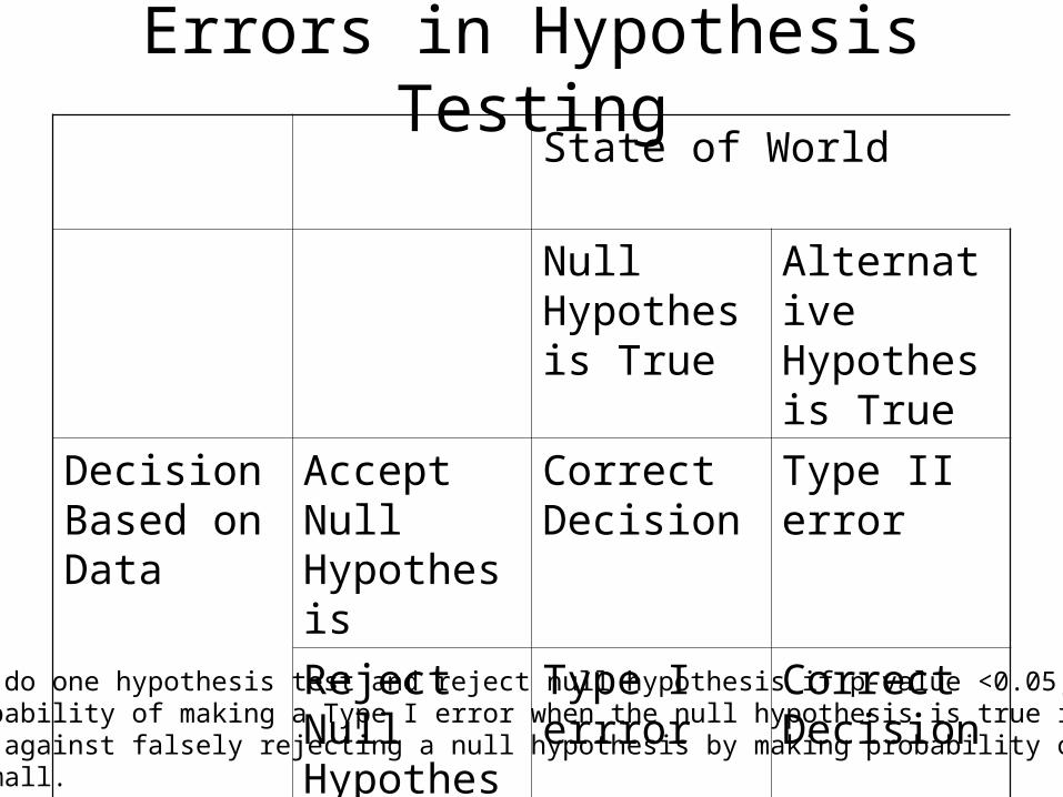
Errors in Hypothesis TestingState of World

Null Hypothesis True

Alternative Hypothesis True

Decision Based on Data

Accept Null Hypothesis

Correct Decision

Type II error

Reject Null Hypothesis

Type I errror

Correct Decision

When we do one hypothesis test and reject null hypothesis if p-value <0.05, thenthe probability of making a Type I error when the null hypothesis is true is 0.05. Weprotect against falsely rejecting a null hypothesis by making probability of Type I error small.

Multiple Comparisons Problem

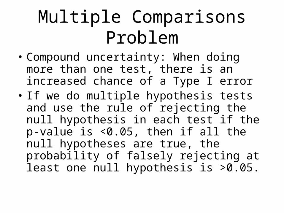
• Compound uncertainty: When doing more than one test, there is an increased chance of a Type I error

• If we do multiple hypothesis tests and use the rule of rejecting the null hypothesis in each test if the p-value is <0.05, then if all the null hypotheses are true, the probability of falsely rejecting at least one null hypothesis is >0.05.

Individual vs. Familywise Error Rate

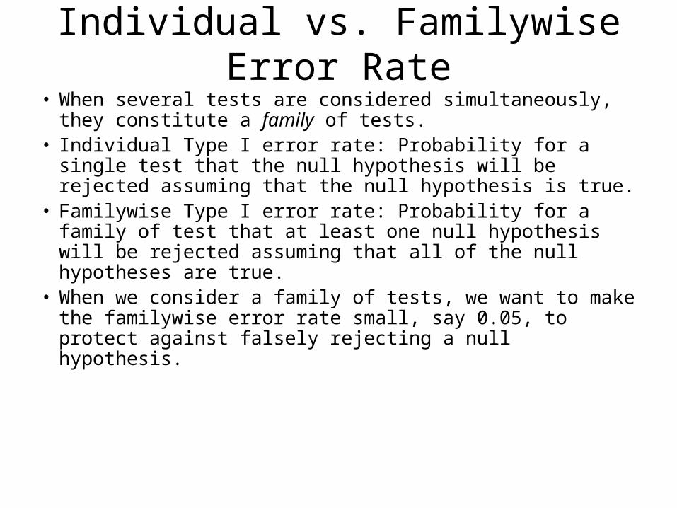
• When several tests are considered simultaneously, they constitute a family of tests.

• Individual Type I error rate: Probability for a single test that the null hypothesis will be rejected assuming that the null hypothesis is true.

• Familywise Type I error rate: Probability for a family of test that at least one null hypothesis will be rejected assuming that all of the null hypotheses are true.

• When we consider a family of tests, we want to make the familywise error rate small, say 0.05, to protect against falsely rejecting a null hypothesis.

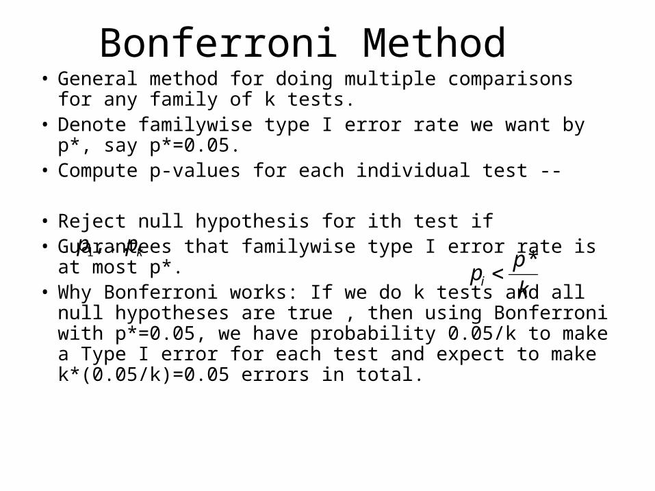
Bonferroni Method• General method for doing multiple comparisons for any

family of k tests. • Denote familywise type I error rate we want by p*, say

p*=0.05. • Compute p-values for each individual test -- • Reject null hypothesis for ith test if• Guarantees that familywise type I error rate is at most p*. • Why Bonferroni works: If we do k tests and all null

hypotheses are true , then using Bonferroni with p*=0.05, we have probability 0.05/k to make a Type I error for each test and expect to make k*(0.05/k)=0.05 errors in total.

kpp ,...,1

k

ppi

*

Bonferroni on Milgram’s Data

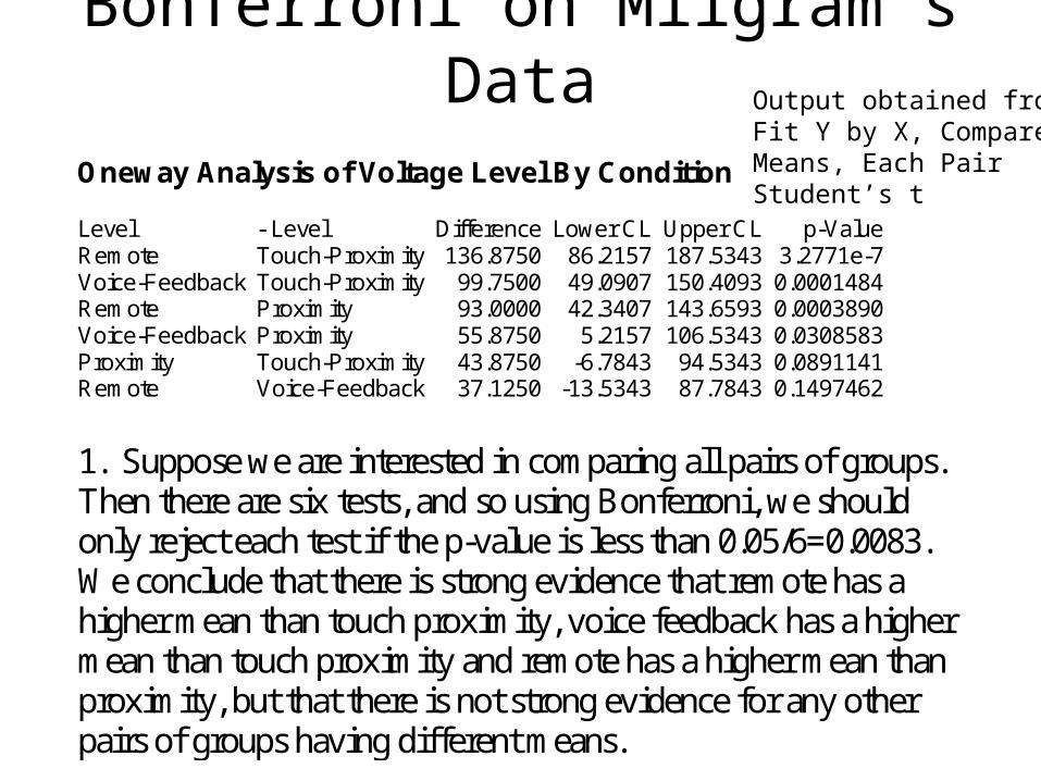
Oneway Analysis of Voltage Level By Condition Level - Level Difference Lower CL Upper CL p-Value Remote Touch-Proximity 136.8750 86.2157 187.5343 3.2771e-7 Voice-Feedback Touch-Proximity 99.7500 49.0907 150.4093 0.0001484 Remote Proximity 93.0000 42.3407 143.6593 0.0003890 Voice-Feedback Proximity 55.8750 5.2157 106.5343 0.0308583 Proximity Touch-Proximity 43.8750 -6.7843 94.5343 0.0891141 Remote Voice-Feedback 37.1250 -13.5343 87.7843 0.1497462

1. Suppose we are interested in comparing all pairs of groups. Then there are six tests, and so using Bonferroni, we should only reject each test if the p-value is less than 0.05/6=0.0083. We conclude that there is strong evidence that remote has a higher mean than touch proximity, voice feedback has a higher mean than touch proximity and remote has a higher mean than proximity, but that there is not strong evidence for any other pairs of groups having different means.

Output obtained fromFit Y by X, CompareMeans, Each Pair Student’s t

Bonferroni on Milgram’s Data Continued

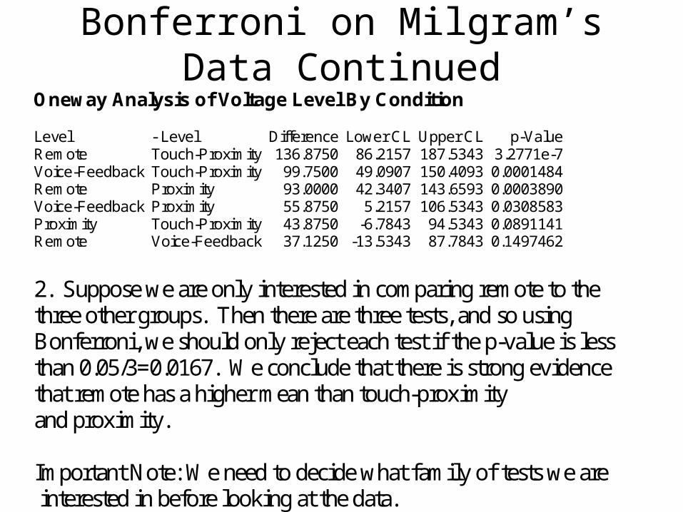
Oneway Analysis of Voltage Level By Condition Level - Level Difference Lower CL Upper CL p-Value Remote Touch-Proximity 136.8750 86.2157 187.5343 3.2771e-7 Voice-Feedback Touch-Proximity 99.7500 49.0907 150.4093 0.0001484 Remote Proximity 93.0000 42.3407 143.6593 0.0003890 Voice-Feedback Proximity 55.8750 5.2157 106.5343 0.0308583 Proximity Touch-Proximity 43.8750 -6.7843 94.5343 0.0891141 Remote Voice-Feedback 37.1250 -13.5343 87.7843 0.1497462

2. Suppose we are only interested in comparing remote to the three other groups. Then there are three tests, and so using Bonferroni, we should only reject each test if the p-value is less than 0.05/3=0.0167. We conclude that there is strong evidence that remote has a higher mean than touch-proximity and proximity. Important Note: We need to decide what family of tests we are interested in before looking at the data.

Tukey’s HSD

• Tukey’s HSD is a method that is specifically designed to control the familywise type I error rate (at 0.05) for analysis of variance when we are interested in comparing all pairs of groups.

• JMP Instructions: After Fit Y by X, click the red triangle next to the X variable and click LSMeans Tukey HSD.

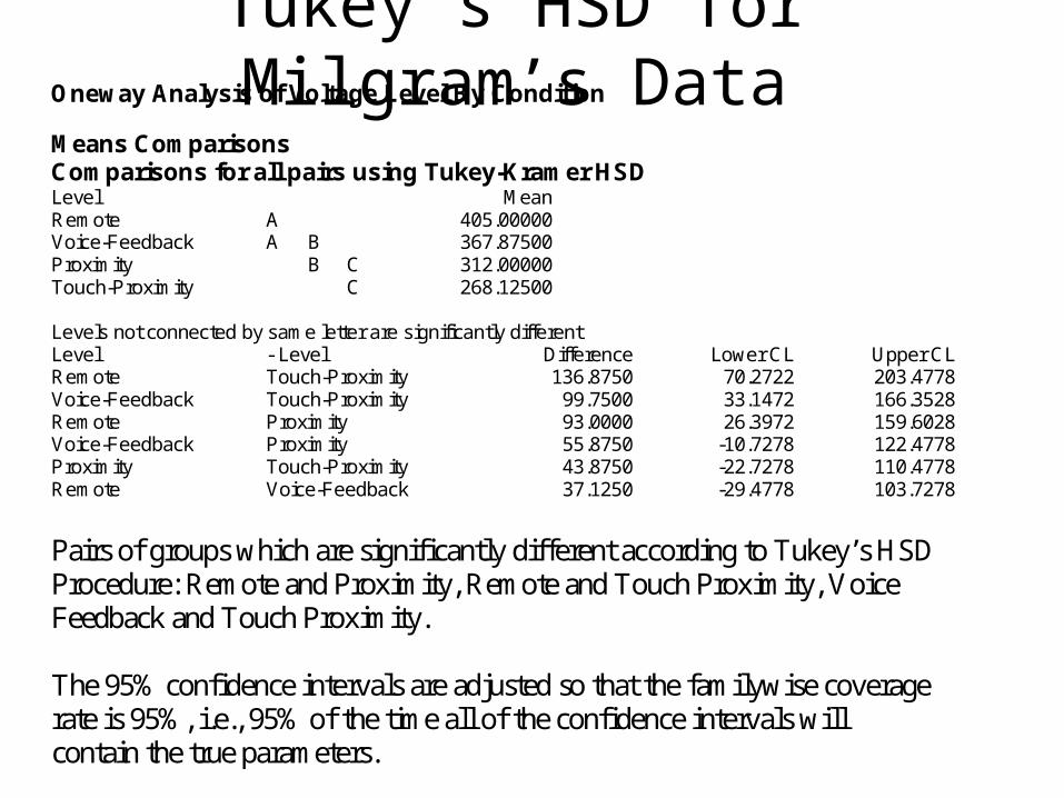
Tukey’s HSD for Milgram’s DataOneway Analysis of Voltage Level By Condition Means Comparisons Comparisons for all pairs using Tukey-Kramer HSD Level Mean Remote A 405.00000 Voice-Feedback A B 367.87500 Proximity B C 312.00000 Touch-Proximity C 268.12500 Levels not connected by same letter are significantly different Level - Level Difference Lower CL Upper CL Remote Touch-Proximity 136.8750 70.2722 203.4778 Voice-Feedback Touch-Proximity 99.7500 33.1472 166.3528 Remote Proximity 93.0000 26.3972 159.6028 Voice-Feedback Proximity 55.8750 -10.7278 122.4778 Proximity Touch-Proximity 43.8750 -22.7278 110.4778 Remote Voice-Feedback 37.1250 -29.4778 103.7278

Pairs of groups which are significantly different according to Tukey’s HSD Procedure: Remote and Proximity, Remote and Touch Proximity, Voice Feedback and Touch Proximity. The 95% confidence intervals are adjusted so that the familywise coverage rate is 95%, i.e., 95% of the time all of the confidence intervals will contain the true parameters.

Assumptions in one-way ANOVA

• Assumptions needed for validity of one-way analysis of variance p-values and CIs:– Linearity: automatically satisfied.– Constant variance: Spread within each group

is the same.– Normality: Distribution within each group is

normally distributed.– Independence: Sample consists of

independent observations.

Rule of thumb for checking constant variance

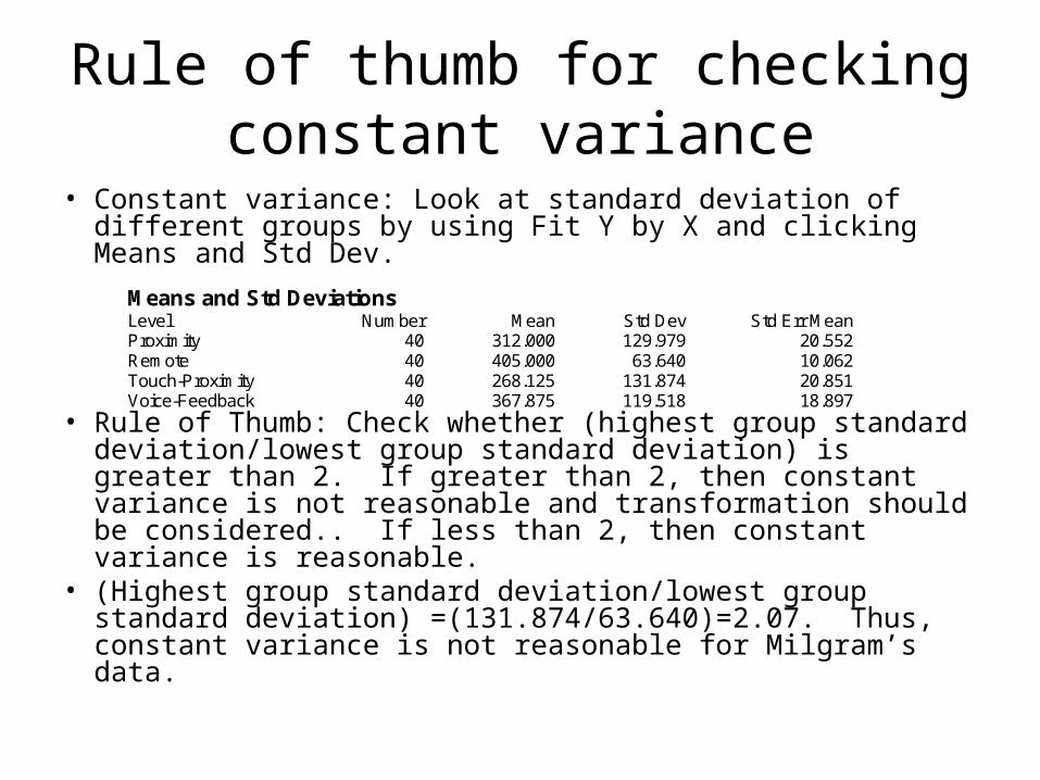
• Constant variance: Look at standard deviation of different groups by using Fit Y by X and clicking Means and Std Dev.

• Rule of Thumb: Check whether (highest group standard deviation/lowest group standard deviation) is greater than 2. If greater than 2, then constant variance is not reasonable and transformation should be considered.. If less than 2, then constant variance is reasonable.

• (Highest group standard deviation/lowest group standard deviation) =(131.874/63.640)=2.07. Thus, constant variance is not reasonable for Milgram’s data.

Means and Std Deviations Level Number Mean Std Dev Std Err Mean Proximity 40 312.000 129.979 20.552 Remote 40 405.000 63.640 10.062 Touch-Proximity 40 268.125 131.874 20.851 Voice-Feedback 40 367.875 119.518 18.897

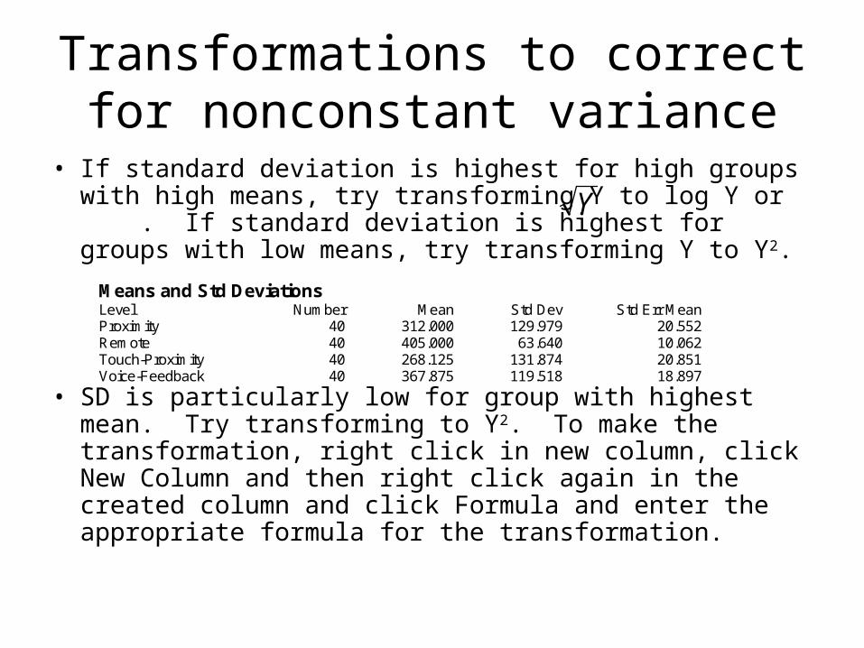
Transformations to correct for nonconstant variance

• If standard deviation is highest for high groups with high means, try transforming Y to log Y or . If standard deviation is highest for groups with low means, try transforming Y to Y2.

• SD is particularly low for group with highest mean. Try transforming to Y2. To make the transformation, right click in new column, click New Column and then right click again in the created column and click Formula and enter the appropriate formula for the transformation.

Y

Means and Std Deviations Level Number Mean Std Dev Std Err Mean Proximity 40 312.000 129.979 20.552 Remote 40 405.000 63.640 10.062 Touch-Proximity 40 268.125 131.874 20.851 Voice-Feedback 40 367.875 119.518 18.897

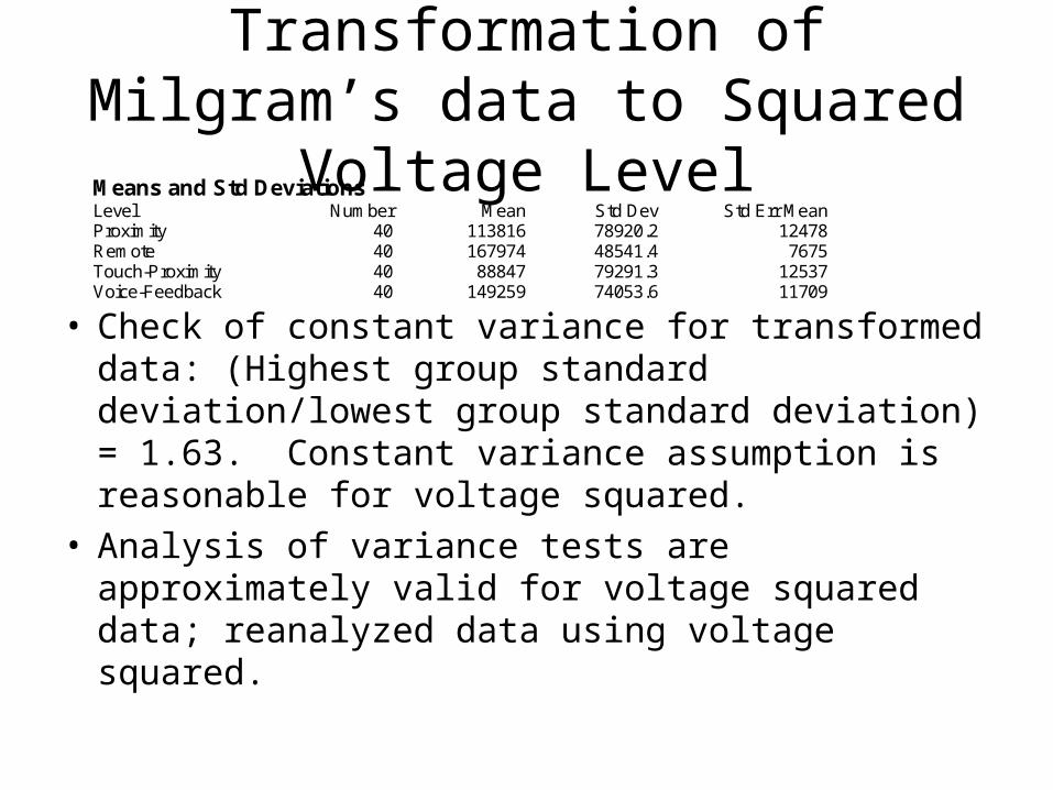
Transformation of Milgram’s data to Squared Voltage Level

• Check of constant variance for transformed data: (Highest group standard deviation/lowest group standard deviation) = 1.63. Constant variance assumption is reasonable for voltage squared.

• Analysis of variance tests are approximately valid for voltage squared data; reanalyzed data using voltage squared.

Means and Std Deviations Level Number Mean Std Dev Std Err Mean Proximity 40 113816 78920.2 12478 Remote 40 167974 48541.4 7675 Touch-Proximity 40 88847 79291.3 12537 Voice-Feedback 40 149259 74053.6 11709

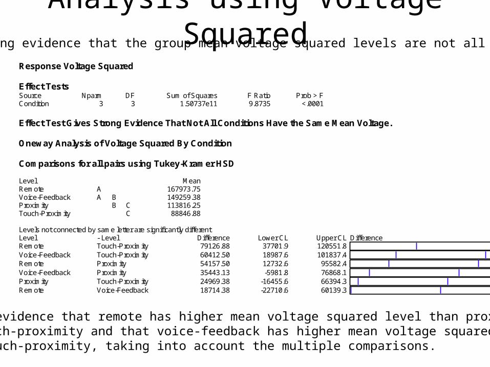
Analysis using Voltage Squared

Response Voltage Squared Effect Tests Source Nparm DF Sum of Squares F Ratio Prob > F Condition 3 3 1.50737e11 9.8735 <.0001 Effect Test Gives Strong Evidence That Not All Conditions Have the Same Mean Voltage. Oneway Analysis of Voltage Squared By Condition Comparisons for all pairs using Tukey-Kramer HSD Level Mean Remote A 167973.75 Voice-Feedback A B 149259.38 Proximity B C 113816.25 Touch-Proximity C 88846.88 Levels not connected by same letter are significantly different Level - Level Difference Lower CL Upper CL Difference Remote Touch-Proximity 79126.88 37701.9 120551.8 Voice-Feedback Touch-Proximity 60412.50 18987.6 101837.4 Remote Proximity 54157.50 12732.6 95582.4 Voice-Feedback Proximity 35443.13 -5981.8 76868.1 Proximity Touch-Proximity 24969.38 -16455.6 66394.3 Remote Voice-Feedback 18714.38 -22710.6 60139.3

Strong evidence that the group mean voltage squared levels are not all the same.

Strong evidence that remote has higher mean voltage squared level than proximityand touch-proximity and that voice-feedback has higher mean voltage squared level than touch-proximity, taking into account the multiple comparisons.

Rule of Thumb for Checking Normality in ANOVA

• The normality assumption for ANOVA is that the distribution in each group is normal. Can be checked by looking at the boxplot, histogram and normal quantile plot for each group.

• If there are more than 30 observations in each group, then the normality assumption is not important; ANOVA p-values and CIs will still be approximately valid even for nonnormal data if there are more than 30 observations in each group.

• If there are less than 30 observations per group, then we can check normality by clicking Analyze, Distribution and then putting the Y variable in the Y, Columns box and the categorical variable denoting the group in the By box. We can then create normal quantile plots for each group and check that for each group, the points in the normal quantile plot are in the confidence bands. If there is nonnormality, we can try to use a transformation such as log Y and see if the transformed data is approximately normally distributed in each group.

One way Analysis of Variance: Steps in Analysis

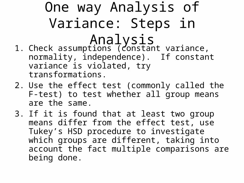
1. Check assumptions (constant variance, normality, independence). If constant variance is violated, try transformations.

2. Use the effect test (commonly called the F-test) to test whether all group means are the same.

3. If it is found that at least two group means differ from the effect test, use Tukey’s HSD procedure to investigate which groups are different, taking into account the fact multiple comparisons are being done.

Analysis of Variance Terminology

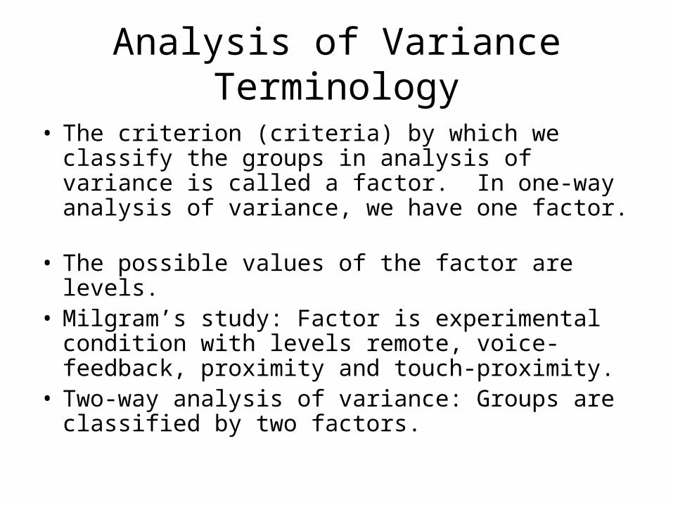
• The criterion (criteria) by which we classify the groups in analysis of variance is called a factor. In one-way analysis of variance, we have one factor.

• The possible values of the factor are levels.• Milgram’s study: Factor is experimental condition

with levels remote, voice-feedback, proximity and touch-proximity.

• Two-way analysis of variance: Groups are classified by two factors.

Two-way Analysis of Variance Examples

• Milgram’s study: In thinking about the Obedience to Authority study, many people have thought that women would react differently than men. Two-way analysis of variance setup in which the two factors are experimental condition (levels remote, voice-feedback, proximity, touch-proximity) and sex (levels male, female).

• Package Design Experiment: Several new types of cereal packages were designed. Two colors and two styles of lettering were considering. Each combination of lettering/color was used to produce a package, and each of these combinations was test marketed in 12 comparable stores and sales in the stores were recorded.. Two-way analysis of variance in which two factors are color (levels red, green) and lettering (levels block, script).

• Goal of two-way analysis of variance: Find out how the mean response in a group depends on the levels of both factors and find the best combination.

Two-way Analysis of Variance

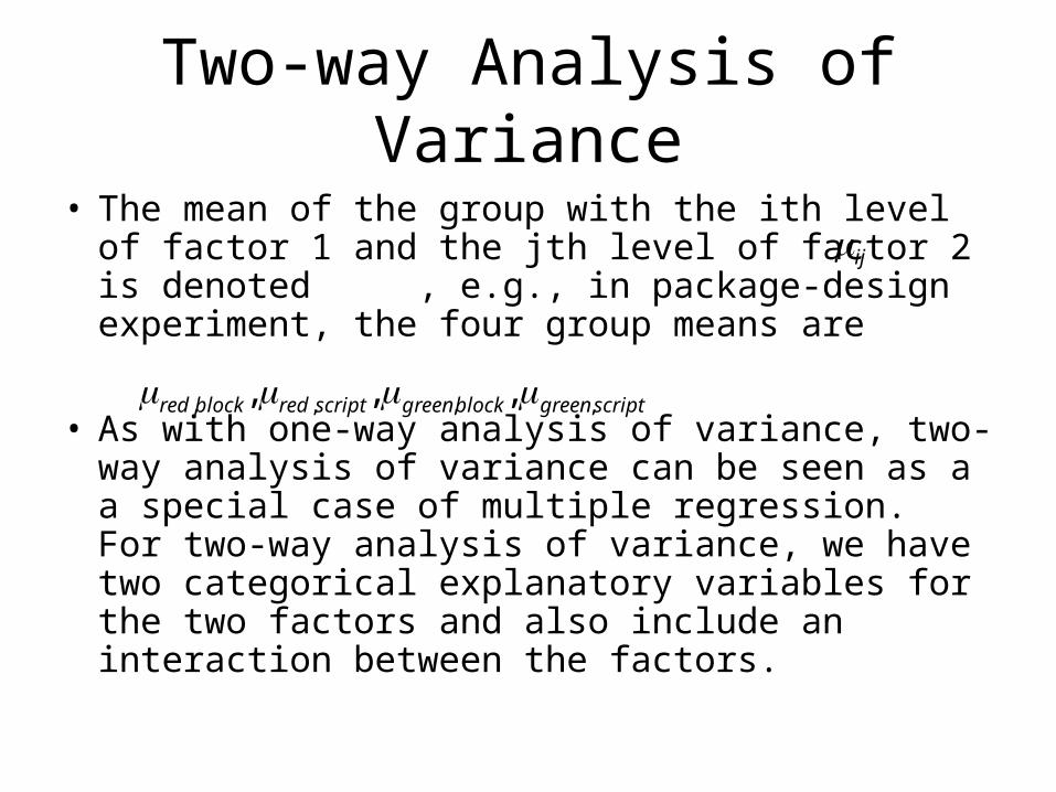
• The mean of the group with the ith level of factor 1 and the jth level of factor 2 is denoted , e.g., in package-design experiment, the four group means are

• As with one-way analysis of variance, two-way analysis of variance can be seen as a a special case of multiple regression. For two-way analysis of variance, we have two categorical explanatory variables for the two factors and also include an interaction between the factors.

ij

scriptgreenblockgreenscriptredblockred ,,,, ,,,

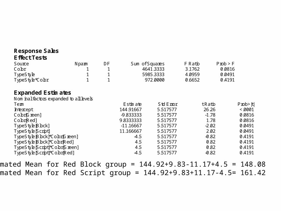
Response Sales Effect Tests Source Nparm DF Sum of Squares F Ratio Prob > F Color 1 1 4641.3333 3.1762 0.0816 TypeStyle 1 1 5985.3333 4.0959 0.0491 TypeStyle*Color 1 1 972.0000 0.6652 0.4191 Expanded Estimates Nominal factors expanded to all levels Term Estimate Std Error t Ratio Prob>|t| Intercept 144.91667 5.517577 26.26 <.0001 Color[Green] -9.833333 5.517577 -1.78 0.0816 Color[Red] 9.8333333 5.517577 1.78 0.0816 TypeStyle[Block] -11.16667 5.517577 -2.02 0.0491 TypeStyle[Script] 11.166667 5.517577 2.02 0.0491 TypeStyle[Block]*Color[Green] -4.5 5.517577 -0.82 0.4191 TypeStyle[Block]*Color[Red] 4.5 5.517577 0.82 0.4191 TypeStyle[Script]*Color[Green] 4.5 5.517577 0.82 0.4191 TypeStyle[Script]*Color[Red] -4.5 5.517577 -0.82 0.4191

Estimated Mean for Red Block group = 144.92+9.83-11.17+4.5 = 148.08Estimated Mean for Red Script group = 144.92+9.83+11.17-4.5= 161.42

LS Means Plot

Sal

esLS

Mea

ns

50

100

150

200

250

Green Red

Color

LS Means Plot

Sal

esLS

Mea

ns

50

100

150

200

250

Block Script

TypeStyle

LS Means Plot

Sal

esLS

Mea

ns

50

100

150

200

250

BlockScript

Green Red

Color

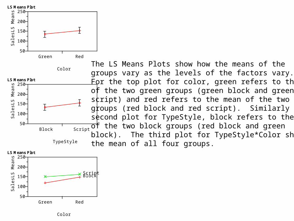
The LS Means Plots show how the means of thegroups vary as the levels of the factors vary.For the top plot for color, green refers to the meanof the two green groups (green block and greenscript) and red refers to the mean of the two redgroups (red block and red script). Similarly for thesecond plot for TypeStyle, block refers to the meanof the two block groups (red block and green block). The third plot for TypeStyle*Color showsthe mean of all four groups.

Two-way ANOVA in JMP

• Use Analyze, Fit Model with a categorical variable for the first factor, a categorical variable for the second factor and an interaction variable that crosses the first factor and the second factor.

• The LS Means Plots are produced by going to the output in JMP for each variable that is to the right of the main output, clicking the red triangle next to each variable (for package design, the vairables are Color, TypeStyle, Typestyle*Color) and clicking LS Means Plot.

Interaction in Two-Way ANOVA

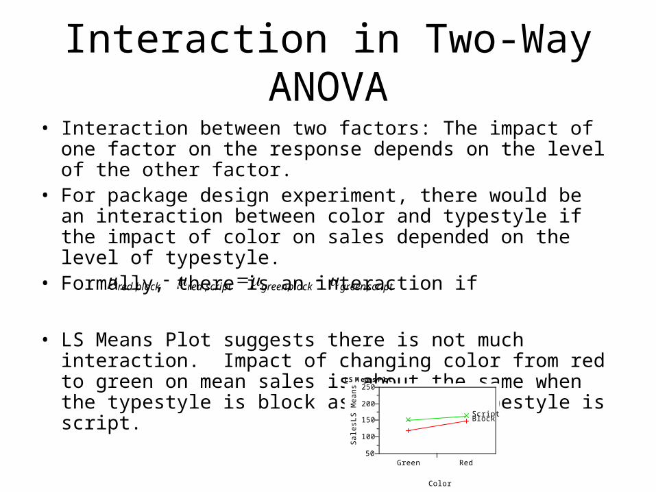
• Interaction between two factors: The impact of one factor on the response depends on the level of the other factor.

• For package design experiment, there would be an interaction between color and typestyle if the impact of color on sales depended on the level of typestyle.

• Formally, there is an interaction if

• LS Means Plot suggests there is not much interaction. Impact of changing color from red to green on mean sales is about the same when the typestyle is block as when the typestyle is script.

LS Means Plot

Sal

esLS

Mea

ns

50

100

150

200

250

BlockScript

Green Red

Color

scriptgreenblockgreenscriptredblockred ,,,,

Effect Test for Interaction

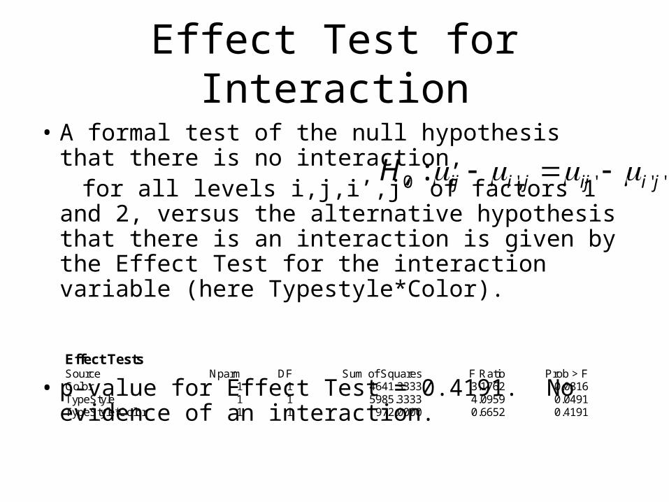
• A formal test of the null hypothesis that there is no interaction,

for all levels i,j,i’,j’ of factors 1 and 2, versus the alternative hypothesis that there is an interaction is given by the Effect Test for the interaction variable (here Typestyle*Color).

• p-value for Effect Test = 0.4191. No evidence of an interaction.

''','0 : jiijjiijH

Effect Tests Source Nparm DF Sum of Squares F Ratio Prob > F Color 1 1 4641.3333 3.1762 0.0816 TypeStyle 1 1 5985.3333 4.0959 0.0491 TypeStyle*Color 1 1 972.0000 0.6652 0.4191

Implications of No Interaction

• When there is no interaction, the two factors can be looked in isolation, one at a time.

• When there is no interaction, best group is determined by finding best level of factor 1 and best level of factor 2 separately.

• For package design experiment, suppose there are two separate groups: one with an expertise in lettering and the other with expertise in coloring. If there is no interaction, groups can work independently to decide best letter and color. If there is an interaction, groups need to get together to decide on best combination of letter and color.

Model when There is No Interaction

• When there is no evidence of an interaction, we can drop the interaction term from the model for parsimony and more accurate estimates:Response Sales Effect Tests Source Nparm DF Sum of Squares F Ratio Prob > F Color 1 1 4641.3333 3.2000 0.0804 TypeStyle 1 1 5985.3333 4.1266 0.0481 Expanded Estimates Nominal factors expanded to all levels Term Estimate Std Error t Ratio Prob>|t| Intercept 144.91667 5.497011 26.36 <.0001 Color[Green] -9.833333 5.497011 -1.79 0.0804 Color[Red] 9.8333333 5.497011 1.79 0.0804 TypeStyle[Block] -11.16667 5.497011 -2.03 0.0481 TypeStyle[Script] 11.166667 5.497011 2.03 0.0481

Mean for red block group = 144.92+9.83-11.17=143.58Mean for red script group = 144.92+9.83+11.17=165.92

Tests for Main Effects When There is No Interaction

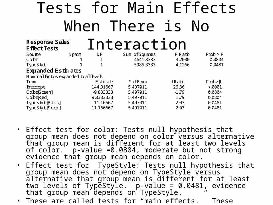
• Effect test for color: Tests null hypothesis that group mean does not depend on color versus alternative that group mean is different for at least two levels of color. p-value =0.0804, moderate but not strong evidence that group mean depends on color.

• Effect test for TypeStyle: Tests null hypothesis that group mean does not depend on TypeStyle versus alternative that group mean is different for at least two levels of TypeStyle. p-value = 0.0481, evidence that group mean depends on TypeStyle.

• These are called tests for “main effects.” These tests only make sense when there is no interaction.

Response Sales Effect Tests Source Nparm DF Sum of Squares F Ratio Prob > F Color 1 1 4641.3333 3.2000 0.0804 TypeStyle 1 1 5985.3333 4.1266 0.0481 Expanded Estimates Nominal factors expanded to all levels Term Estimate Std Error t Ratio Prob>|t| Intercept 144.91667 5.497011 26.36 <.0001 Color[Green] -9.833333 5.497011 -1.79 0.0804 Color[Red] 9.8333333 5.497011 1.79 0.0804 TypeStyle[Block] -11.16667 5.497011 -2.03 0.0481 TypeStyle[Script] 11.166667 5.497011 2.03 0.0481

Example with an Interaction

• Should the clerical employees of a large insurance company be switched to a four-day week, allowed to use flextime schedules or kept to the usual 9-to-5 workday?

• The data set flextime.JMP contains percentage efficiency gains over a four week trial period for employees grouped by two factors: Department (Claims, Data Processing, Investment) and Condition (Flextime, Four-day week, Regular Hours).

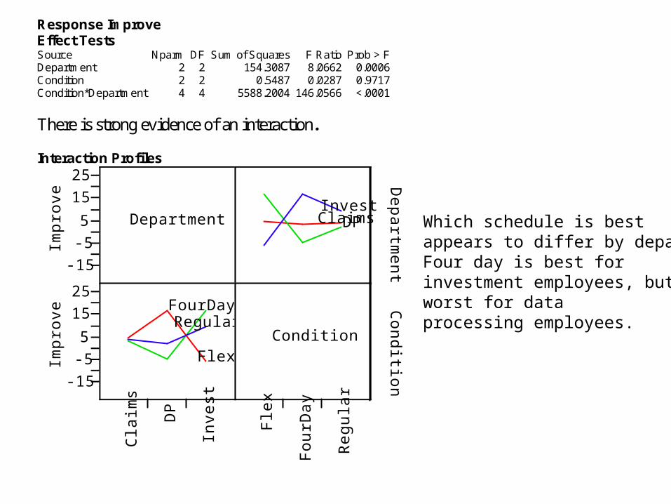
Response Improve Effect Tests Source Nparm DF Sum of Squares F Ratio Prob > F Department 2 2 154.3087 8.0662 0.0006 Condition 2 2 0.5487 0.0287 0.9717 Condition*Department 4 4 5588.2004 146.0566 <.0001 There is strong evidence of an interaction. Interaction Profiles

-15

-5

5

15

25

Impr

ove

-15

-5

5

15

25

Impr

ove

Department

Flex

FourDayRegular

Cla

ims

DP

Inve

stClaimsDPInvest

Condition

Fle

x

Fou

rDay

Reg

ular

Departm

entC

ondition

Which schedule is best appears to differ by department.Four day is best for investment employees, but worst for data processing employees.

Which Combinations Works Best?

• For which pairs of groups is there strong evidence that the groups have different means – is there strong evidence that one combination works best?

• We combine the two factors into one factor (Combination) and use Tukey’s HSD, to compare groups pairwise, adjusting for multiple comparisons.

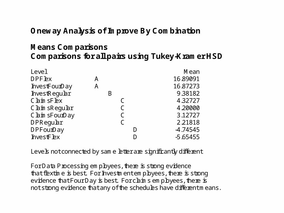
Oneway Analysis of Improve By Combination Means Comparisons Comparisons for all pairs using Tukey-Kramer HSD Level Mean DPFlex A 16.89091 InvestFourDay A 16.87273 InvestRegular B 9.38182 ClaimsFlex C 4.32727 ClaimsRegular C 4.20000 ClaimsFourDay C 3.12727 DPRegular C 2.21818 DPFourDay D -4.74545 InvestFlex D -5.65455 Levels not connected by same letter are significantly different For Data Processing employees, there is strong evidence that flextime is best. For Investment employees, there is strong evidence that Four Day is best. For claims employees, there is not strong evidence that any of the schedules have different means.

Checking Assumptions

• As with one-way ANOVA, two-way ANOVA is a special case of multiple regression and relies on the assumptions: – Linearity: Automatically satisfied– Constant variance: Spread within groups is the same

for all groups.– Normality: Distribution within each group is normal.

• To check assumptions, combine two factors into one factor (Combination) and check assumptions as in one-way ANOVA.

Checking Assumptions

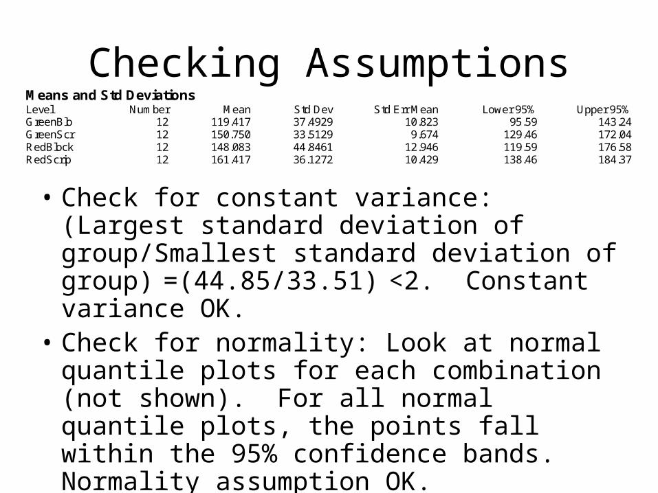
• Check for constant variance: (Largest standard deviation of group/Smallest standard deviation of group)

=(44.85/33.51) <2. Constant variance OK.• Check for normality: Look at normal

quantile plots for each combination (not shown). For all normal quantile plots, the points fall within the 95% confidence bands. Normality assumption OK.

Means and Std Deviations Level Number Mean Std Dev Std Err Mean Lower 95% Upper 95% GreenBlo 12 119.417 37.4929 10.823 95.59 143.24 GreenScr 12 150.750 33.5129 9.674 129.46 172.04 RedBlock 12 148.083 44.8461 12.946 119.59 176.58 RedScrip 12 161.417 36.1272 10.429 138.46 184.37

Two way Analysis of Variance: Steps in Analysis

1. Check assumptions (constant variance, normality, independence). If constant variance is violated, try transformations.

2. Use the effect test (commonly called the F-test) to test whether there is an interaction.

3. If there is no interaction, use the main effect tests to whether each factor has an effect. Compare individual levels of a factor by using t-tests with Bonferroni correction for the number of comparisons being made.

4. If there is an interaction, use the interaction plot to visualize the interaction. Create combination of the factors and use Tukey’s HSD procedure to investigate which groups are different, taking into account the fact multiple comparisons are being done.