Embed Size (px)
Citation preview

STAT 380
Markov Chains
Richard Lockhart
Simon Fraser University
Spring 2016
Richard Lockhart (Simon Fraser University) STAT 380 Markov Chains Spring 2016 1 / 76
Markov Chains
Last names example has following structure:
Suppose, at generation n there are m individuals.
Number of sons in next generation has distribution of sum of mindependent copies of rv X
Recall X is number of sons in first generation.
Distribution does not depend on n,
Depends only on the value m of Zn.
We call Zn a Markov Chain.
Richard Lockhart (Simon Fraser University) STAT 380 Markov Chains Spring 2016 2 / 76
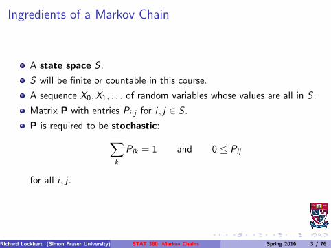
Ingredients of a Markov Chain
A state space S .
S will be finite or countable in this course.
A sequence X0,X1, . . . of random variables whose values are all in S .
Matrix P with entries Pi ,j for i , j ∈ S .
P is required to be stochastic:
∑
k
Pik = 1 and 0 ≤ Pij
for all i , j .
Richard Lockhart (Simon Fraser University) STAT 380 Markov Chains Spring 2016 3 / 76
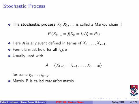
Stochastic Process
The stochastic process X0,X1, . . . is called a Markov chain if
P (Xk+1 = j |Xk = i ,A) = Pi ,j
Here A is any event defined in terms of X0, . . . ,Xk−1.
Formula must hold for all i , j , k .
Usually used with
A = {Xk−1 = ik−1, . . . ,X0 = i0}
for some i0, . . . , ik−1.
Matrix P is called transition matrix.
Richard Lockhart (Simon Fraser University) STAT 380 Markov Chains Spring 2016 4 / 76
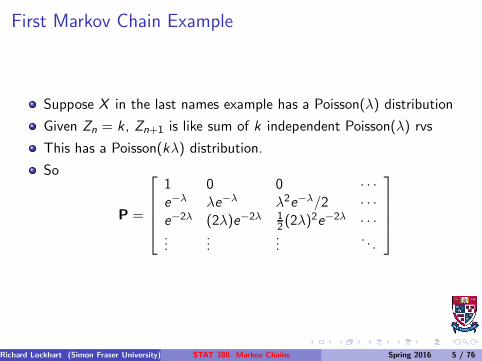
First Markov Chain Example
Suppose X in the last names example has a Poisson(λ) distribution
Given Zn = k , Zn+1 is like sum of k independent Poisson(λ) rvs
This has a Poisson(kλ) distribution.
So
P =
1 0 0 · · ·e−λ λe−λ λ2e−λ/2 · · ·e−2λ (2λ)e−2λ 1
2 (2λ)2e−2λ · · ·
......
.... . .
Richard Lockhart (Simon Fraser University) STAT 380 Markov Chains Spring 2016 5 / 76
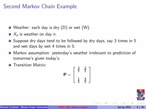
Second Markov Chain Example
Weather: each day is dry (D) or wet (W).
Xn is weather on day n.
Suppose dry days tend to be followed by dry days, say 3 times in 5and wet days by wet 4 times in 5.
Markov assumption: yesterday’s weather irrelevant to prediction oftomorrow’s given today’s.
Transition Matrix:
P =
35
25
15
45
Richard Lockhart (Simon Fraser University) STAT 380 Markov Chains Spring 2016 6 / 76
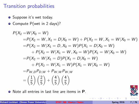
Transition probabilities
Suppose it’s wet today.
Compute P(wet in 2 days)?
P(X2 =W |X0 = W )
=P(X2 = W ,X1 = D|X0 = W ) + P(X2 = W ,X1 = W |X0 = W )
=P(X2 = W |X1 = D,X0 = W )P(X1 = D|X0 = W )
+ P(X2 = W |X1 = W ,X0 = W )P(X1 = W |X0 = W )
=P(X2 = W |X1 = D)P(X1 = D|X0 = W )
+ P(X2 = W |X1 = W )P(X1 = W |X0 = W )
=PW ,DPD,W + PW ,WPW ,W
=
(
1
5
)(
2
5
)
+
(
4
5
)(
4
5
)
Note all entries in last line are items in P.
Richard Lockhart (Simon Fraser University) STAT 380 Markov Chains Spring 2016 7 / 76
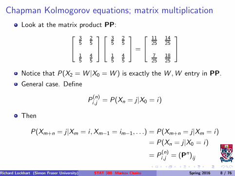
Chapman Kolmogorov equations; matrix multiplication
Look at the matrix product PP:
35
25
15
45
35
25
15
45
=
1125
1425
725
1825
Notice that P(X2 = W |X0 = W ) is exactly the W ,W entry in PP.
General case. Define
P(n)i ,j = P(Xn = j |X0 = i)
Then
P(Xm+n = j |Xm = i ,Xm−1 = im−1, . . .) = P(Xm+n = j |Xm = i)
= P(Xn = j |X0 = i)
= P(n)i ,j = (Pn)ij
Richard Lockhart (Simon Fraser University) STAT 380 Markov Chains Spring 2016 8 / 76
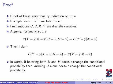
Proof
Proof of these assertions by induction on m, n.
Example for n = 2. Two bits to do:
First suppose U,V ,X ,Y are discrete variables.
Assume: for any x , y , u, v
P(Y = y |X = x ,U = u,V = v) = P(Y = y |X = x)
Then I claim
P(Y = y |X = x ,U = u) = P(Y = y |X = x)
In words, if knowing both U and V doesn’t change the conditionalprobability then knowing U alone doesn’t change the conditionalprobability.
Richard Lockhart (Simon Fraser University) STAT 380 Markov Chains Spring 2016 9 / 76
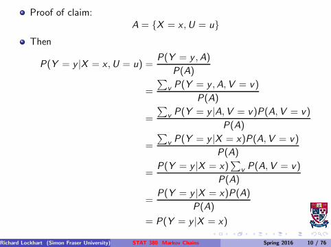
Proof of claim:A = {X = x ,U = u}
Then
P(Y = y |X = x ,U = u) =P(Y = y ,A)
P(A)
=
∑
v P(Y = y ,A,V = v)
P(A)
=
∑
v P(Y = y |A,V = v)P(A,V = v)
P(A)
=
∑
v P(Y = y |X = x)P(A,V = v)
P(A)
=P(Y = y |X = x)
∑
v P(A,V = v)
P(A)
=P(Y = y |X = x)P(A)
P(A)
= P(Y = y |X = x)
Richard Lockhart (Simon Fraser University) STAT 380 Markov Chains Spring 2016 10 / 76
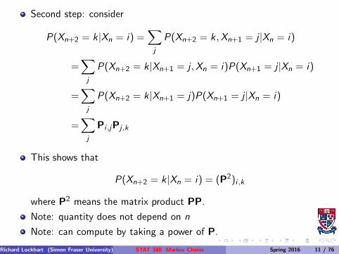
Second step: consider
P(Xn+2 = k |Xn = i) =∑
j
P(Xn+2 = k ,Xn+1 = j |Xn = i)
=∑
j
P(Xn+2 = k |Xn+1 = j ,Xn = i)P(Xn+1 = j |Xn = i)
=∑
j
P(Xn+2 = k |Xn+1 = j)P(Xn+1 = j |Xn = i)
=∑
j
Pi ,jPj ,k
This shows that
P(Xn+2 = k |Xn = i) = (P2)i ,k
where P2 means the matrix product PP.
Note: quantity does not depend on n
Note: can compute by taking a power of P.
Richard Lockhart (Simon Fraser University) STAT 380 Markov Chains Spring 2016 11 / 76
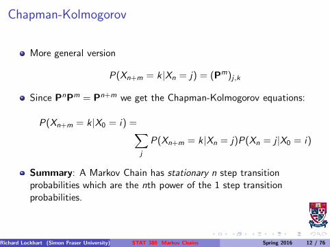
Chapman-Kolmogorov
More general version
P(Xn+m = k |Xn = j) = (Pm)j ,k
Since PnPm = Pn+m we get the Chapman-Kolmogorov equations:
P(Xn+m = k |X0 = i) =∑
j
P(Xn+m = k |Xn = j)P(Xn = j |X0 = i)
Summary: A Markov Chain has stationary n step transitionprobabilities which are the nth power of the 1 step transitionprobabilities.
Richard Lockhart (Simon Fraser University) STAT 380 Markov Chains Spring 2016 12 / 76
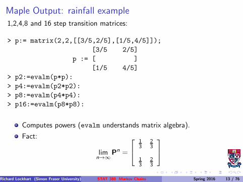
Maple Output: rainfall example
1,2,4,8 and 16 step transition matrices:
> p:= matrix(2,2,[[3/5,2/5],[1/5,4/5]]);
[3/5 2/5]
p := [ ]
[1/5 4/5]
> p2:=evalm(p*p):
> p4:=evalm(p2*p2):
> p8:=evalm(p4*p4):
> p16:=evalm(p8*p8):
Computes powers (evalm understands matrix algebra).
Fact:
limn→∞
Pn =
13
23
13
23
Richard Lockhart (Simon Fraser University) STAT 380 Markov Chains Spring 2016 13 / 76
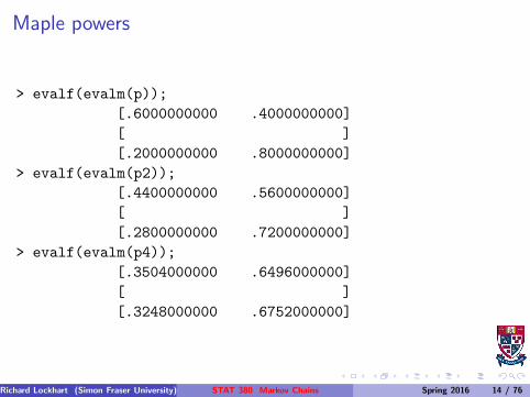
Maple powers
> evalf(evalm(p));
[.6000000000 .4000000000]
[ ]
[.2000000000 .8000000000]
> evalf(evalm(p2));
[.4400000000 .5600000000]
[ ]
[.2800000000 .7200000000]
> evalf(evalm(p4));
[.3504000000 .6496000000]
[ ]
[.3248000000 .6752000000]
Richard Lockhart (Simon Fraser University) STAT 380 Markov Chains Spring 2016 14 / 76
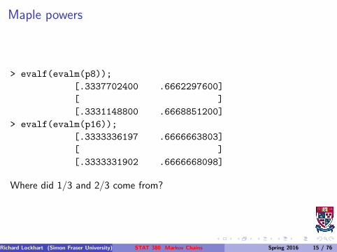
Maple powers
> evalf(evalm(p8));
[.3337702400 .6662297600]
[ ]
[.3331148800 .6668851200]
> evalf(evalm(p16));
[.3333336197 .6666663803]
[ ]
[.3333331902 .6666668098]
Where did 1/3 and 2/3 come from?
Richard Lockhart (Simon Fraser University) STAT 380 Markov Chains Spring 2016 15 / 76
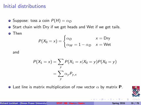
Initial distributions
Suppose: toss a coin P(H) = αD
Start chain with Dry if we get heads and Wet if we get tails.
Then
P(X0 = x) =
{
αD x = Dry
αW = 1− αD x = Wet
and
P(X1 = x) =∑
y
P(X1 = x |X0 = y)P(X0 = y)
=∑
y
αyPy ,x
Last line is matrix multiplication of row vector α by matrix P.
Richard Lockhart (Simon Fraser University) STAT 380 Markov Chains Spring 2016 16 / 76
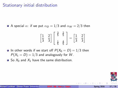
Stationary initial distribution
A special α: if we put αD = 1/3 and αW = 2/3 then
[
1
3
2
3
]
35
25
15
45
=
[
1
3
2
3
]
In other words if we start off P(X0 = D) = 1/3 thenP(X1 = D) = 1/3 and analogously for W .
So X0 and X1 have the same distribution.
Richard Lockhart (Simon Fraser University) STAT 380 Markov Chains Spring 2016 17 / 76
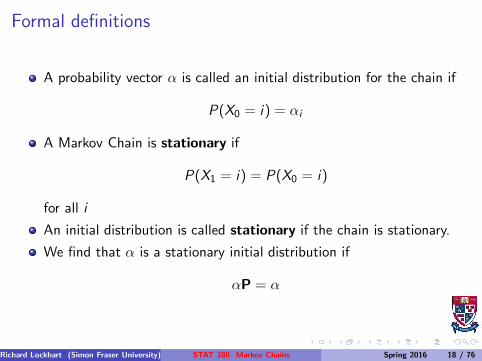
Formal definitions
A probability vector α is called an initial distribution for the chain if
P(X0 = i) = αi
A Markov Chain is stationary if
P(X1 = i) = P(X0 = i)
for all i
An initial distribution is called stationary if the chain is stationary.
We find that α is a stationary initial distribution if
αP = α
Richard Lockhart (Simon Fraser University) STAT 380 Markov Chains Spring 2016 18 / 76
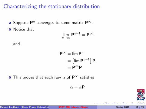
Characterizing the stationary distribution
Suppose Pn converges to some matrix P∞.
Notice thatlimn→∞
Pn−1 = P∞
and
P∞ = limPn
=[
limPn−1]
P
= P∞P
This proves that each row α of P∞ satisfies
α = αP
Richard Lockhart (Simon Fraser University) STAT 380 Markov Chains Spring 2016 19 / 76
Eigenvectors
Def’n: A row vector x is a left eigenvector of A with eigenvalue λ if
xA = λx
So each row of P∞ is a left eigenvector of P with eigenvalue 1.
Richard Lockhart (Simon Fraser University) STAT 380 Markov Chains Spring 2016 20 / 76
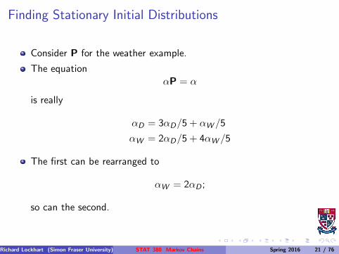
Finding Stationary Initial Distributions
Consider P for the weather example.
The equationαP = α
is really
αD = 3αD/5 + αW /5
αW = 2αD/5 + 4αW /5
The first can be rearranged to
αW = 2αD ;
so can the second.
Richard Lockhart (Simon Fraser University) STAT 380 Markov Chains Spring 2016 21 / 76
Finding Stationary Initial Distributions again
If α is to be a probability vector then
αW + αD = 1
so we get1− αD = 2αD
leading toαD = 1/3
Richard Lockhart (Simon Fraser University) STAT 380 Markov Chains Spring 2016 22 / 76
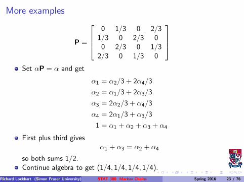
More examples
P =
0 1/3 0 2/31/3 0 2/3 00 2/3 0 1/3
2/3 0 1/3 0
Set αP = α and get
α1 = α2/3 + 2α4/3
α2 = α1/3 + 2α3/3
α3 = 2α2/3 + α4/3
α4 = 2α1/3 + α3/3
1 = α1 + α2 + α3 + α4
First plus third givesα1 + α3 = α2 + α4
so both sums 1/2.Continue algebra to get (1/4, 1/4, 1/4, 1/4).
Richard Lockhart (Simon Fraser University) STAT 380 Markov Chains Spring 2016 23 / 76
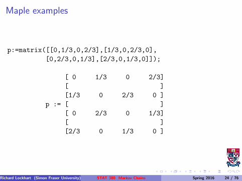
Maple examples
p:=matrix([[0,1/3,0,2/3],[1/3,0,2/3,0],
[0,2/3,0,1/3],[2/3,0,1/3,0]]);
[ 0 1/3 0 2/3]
[ ]
[1/3 0 2/3 0 ]
p := [ ]
[ 0 2/3 0 1/3]
[ ]
[2/3 0 1/3 0 ]
Richard Lockhart (Simon Fraser University) STAT 380 Markov Chains Spring 2016 24 / 76
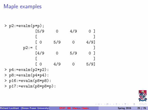
Maple examples
> p2:=evalm(p*p);
[5/9 0 4/9 0 ]
[ ]
[ 0 5/9 0 4/9]
p2:= [ ]
[4/9 0 5/9 0 ]
[ ]
[ 0 4/9 0 5/9]
> p4:=evalm(p2*p2):
> p8:=evalm(p4*p4):
> p16:=evalm(p8*p8):
> p17:=evalm(p8*p8*p):
Richard Lockhart (Simon Fraser University) STAT 380 Markov Chains Spring 2016 25 / 76
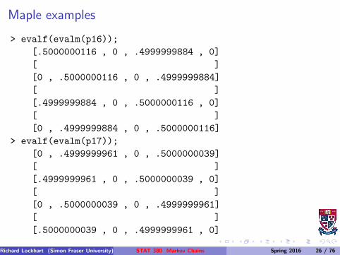
Maple examples
> evalf(evalm(p16));
[.5000000116 , 0 , .4999999884 , 0]
[ ]
[0 , .5000000116 , 0 , .4999999884]
[ ]
[.4999999884 , 0 , .5000000116 , 0]
[ ]
[0 , .4999999884 , 0 , .5000000116]
> evalf(evalm(p17));
[0 , .4999999961 , 0 , .5000000039]
[ ]
[.4999999961 , 0 , .5000000039 , 0]
[ ]
[0 , .5000000039 , 0 , .4999999961]
[ ]
[.5000000039 , 0 , .4999999961 , 0]
Richard Lockhart (Simon Fraser University) STAT 380 Markov Chains Spring 2016 26 / 76
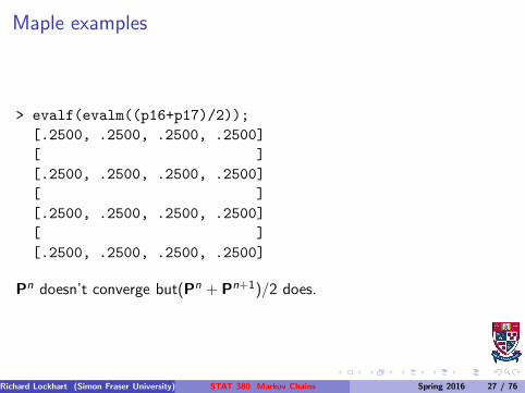
Maple examples
> evalf(evalm((p16+p17)/2));
[.2500, .2500, .2500, .2500]
[ ]
[.2500, .2500, .2500, .2500]
[ ]
[.2500, .2500, .2500, .2500]
[ ]
[.2500, .2500, .2500, .2500]
Pn doesn’t converge but(Pn + Pn+1)/2 does.
Richard Lockhart (Simon Fraser University) STAT 380 Markov Chains Spring 2016 27 / 76
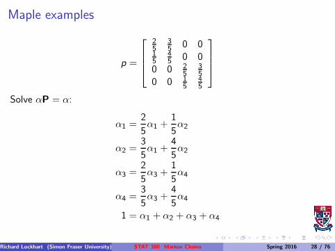
Maple examples
p =
25
35 0 0
15
45 0 0
0 0 25
35
0 0 15
45
Solve αP = α:
α1 =2
5α1 +
1
5α2
α2 =3
5α1 +
4
5α2
α3 =2
5α3 +
1
5α4
α4 =3
5α3 +
4
5α4
1 = α1 + α2 + α3 + α4
Richard Lockhart (Simon Fraser University) STAT 380 Markov Chains Spring 2016 28 / 76
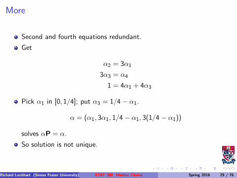
More
Second and fourth equations redundant.
Get
α2 = 3α1
3α3 = α4
1 = 4α1 + 4α3
Pick α1 in [0, 1/4]; put α3 = 1/4− α1.
α = (α1, 3α1, 1/4 − α1, 3(1/4 − α1))
solves αP = α.
So solution is not unique.
Richard Lockhart (Simon Fraser University) STAT 380 Markov Chains Spring 2016 29 / 76
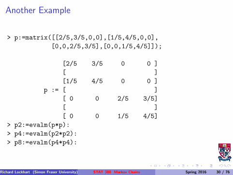
Another Example
> p:=matrix([[2/5,3/5,0,0],[1/5,4/5,0,0],
[0,0,2/5,3/5],[0,0,1/5,4/5]]);
[2/5 3/5 0 0 ]
[ ]
[1/5 4/5 0 0 ]
p := [ ]
[ 0 0 2/5 3/5]
[ ]
[ 0 0 1/5 4/5]
> p2:=evalm(p*p):
> p4:=evalm(p2*p2):
> p8:=evalm(p4*p4):
Richard Lockhart (Simon Fraser University) STAT 380 Markov Chains Spring 2016 30 / 76
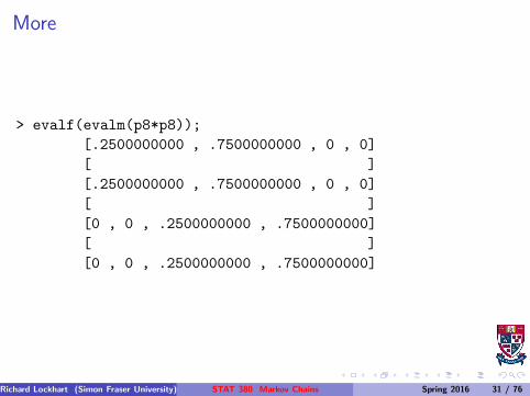
More
> evalf(evalm(p8*p8));
[.2500000000 , .7500000000 , 0 , 0]
[ ]
[.2500000000 , .7500000000 , 0 , 0]
[ ]
[0 , 0 , .2500000000 , .7500000000]
[ ]
[0 , 0 , .2500000000 , .7500000000]
Richard Lockhart (Simon Fraser University) STAT 380 Markov Chains Spring 2016 31 / 76
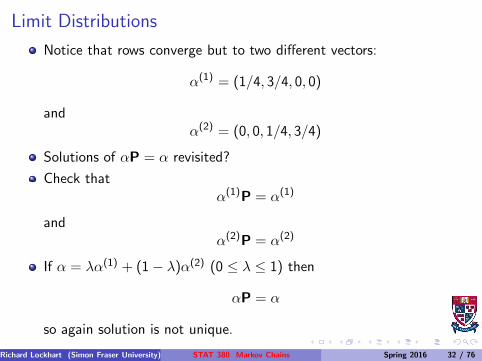
Limit Distributions
Notice that rows converge but to two different vectors:
α(1) = (1/4, 3/4, 0, 0)
andα(2) = (0, 0, 1/4, 3/4)
Solutions of αP = α revisited?
Check thatα(1)P = α(1)
andα(2)P = α(2)
If α = λα(1) + (1− λ)α(2) (0 ≤ λ ≤ 1) then
αP = α
so again solution is not unique.
Richard Lockhart (Simon Fraser University) STAT 380 Markov Chains Spring 2016 32 / 76
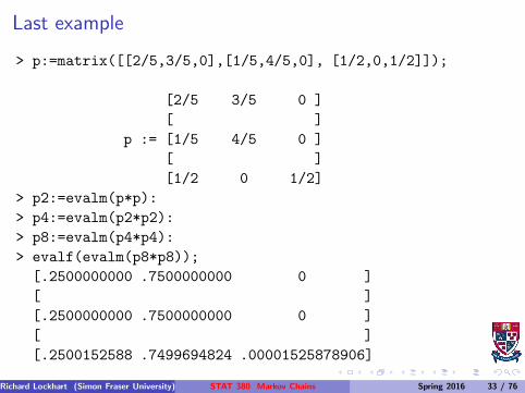
Last example
> p:=matrix([[2/5,3/5,0],[1/5,4/5,0], [1/2,0,1/2]]);
[2/5 3/5 0 ]
[ ]
p := [1/5 4/5 0 ]
[ ]
[1/2 0 1/2]
> p2:=evalm(p*p):
> p4:=evalm(p2*p2):
> p8:=evalm(p4*p4):
> evalf(evalm(p8*p8));
[.2500000000 .7500000000 0 ]
[ ]
[.2500000000 .7500000000 0 ]
[ ]
[.2500152588 .7499694824 .00001525878906]
Richard Lockhart (Simon Fraser University) STAT 380 Markov Chains Spring 2016 33 / 76
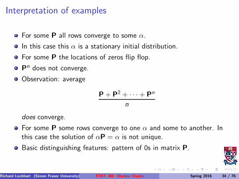
Interpretation of examples
For some P all rows converge to some α.
In this case this α is a stationary initial distribution.
For some P the locations of zeros flip flop.
Pn does not converge.
Observation: average
P+ P2 + · · ·+ Pn
n
does converge.
For some P some rows converge to one α and some to another. Inthis case the solution of αP = α is not unique.
Basic distinguishing features: pattern of 0s in matrix P.
Richard Lockhart (Simon Fraser University) STAT 380 Markov Chains Spring 2016 34 / 76
Classification of States
State i leads to state j if Pnij > 0 for some n.
Convenient to agree say P0 = I, the identity matrix.
So i leads to i .
Note i leads to j and j leads to k implies i leads to k
(Chapman-Kolmogorov).
States i and j communicate if i leads to j and j leads to i .
The relation of communication is an equivalence relation.
it is reflexive, symmetric and transitive: if i and j communicate and j
and k communicate then i and k communicate.
Group of communicating states called Communicating Class.
Richard Lockhart (Simon Fraser University) STAT 380 Markov Chains Spring 2016 35 / 76
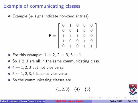
Example of communicating classes
Example (+ signs indicate non-zero entries):
P =
0 1 0 0 00 0 1 0 0+ + + 0 0+ 0 0 + 00 + 0 + +
For this example: 1 2, 2 3, 3 1
So 1, 2, 3 are all in the same communicating class.
4 1, 2, 3 but not vice versa.
5 1, 2, 3, 4 but not vice versa.
So the communicating classes are
{1, 2, 3} {4} {5}
Richard Lockhart (Simon Fraser University) STAT 380 Markov Chains Spring 2016 36 / 76
Irreducible Chains, transience, recurrence
A Markov Chain is irreducible if there is only one communicatingclass.
Notation:fi = P(∃n > 0 : Xn = i |X0 = i)
State i is recurrent if fi = 1, otherwise transient.
If fi = 1 then Markov property (chain starts over when it gets back toi) means prob return infinitely many times (given started in i or givenever get to i) is 1.
Richard Lockhart (Simon Fraser University) STAT 380 Markov Chains Spring 2016 37 / 76
Number of returns to transient state
Consider chain started from transient i .
Let N be number of visits to state i (including visit at time 0).
To return m times must return once then starting over return m − 1times, then never return.
So:P(N = m|X0 = i) = f m−1
i (1− fi)
for m = 1, 2, . . ..
N has a Geometric distribution and E(N|X0 = i) = 1/(1 − fi).
Richard Lockhart (Simon Fraser University) STAT 380 Markov Chains Spring 2016 38 / 76
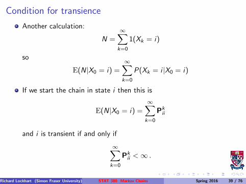
Condition for transience
Another calculation:
N =∞∑
k=0
1(Xk = i)
so
E(N|X0 = i) =
∞∑
k=0
P(Xk = i |X0 = i)
If we start the chain in state i then this is
E(N|X0 = i) =
∞∑
k=0
Pkii
and i is transient if and only if
∞∑
k=0
Pkii < ∞ .
Richard Lockhart (Simon Fraser University) STAT 380 Markov Chains Spring 2016 39 / 76
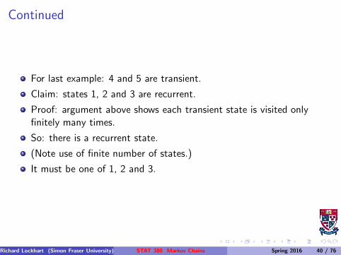
Continued
For last example: 4 and 5 are transient.
Claim: states 1, 2 and 3 are recurrent.
Proof: argument above shows each transient state is visited onlyfinitely many times.
So: there is a recurrent state.
(Note use of finite number of states.)
It must be one of 1, 2 and 3.
Richard Lockhart (Simon Fraser University) STAT 380 Markov Chains Spring 2016 40 / 76
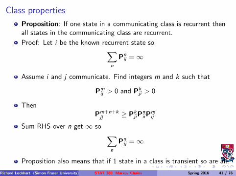
Class properties
Proposition: If one state in a communicating class is recurrent thenall states in the communicating class are recurrent.
Proof: Let i be the known recurrent state so∑
n
Pnii = ∞
Assume i and j communicate. Find integers m and k such that
Pmij > 0 and Pk
ji > 0
ThenPm+n+kjj ≥ Pk
jiPniiP
mij
Sum RHS over n get ∞ so∑
n
Pnjj = ∞
Proposition also means that if 1 state in a class is transient so are all.
Richard Lockhart (Simon Fraser University) STAT 380 Markov Chains Spring 2016 41 / 76
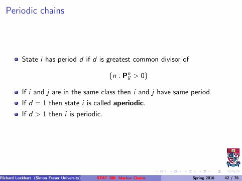
Periodic chains
State i has period d if d is greatest common divisor of
{n : Pnii > 0}
If i and j are in the same class then i and j have same period.
If d = 1 then state i is called aperiodic.
If d > 1 then i is periodic.
Richard Lockhart (Simon Fraser University) STAT 380 Markov Chains Spring 2016 42 / 76
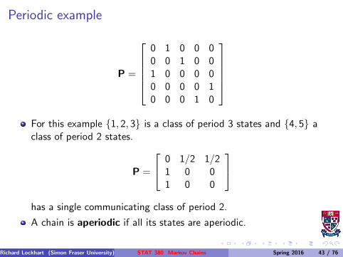
Periodic example
P =
0 1 0 0 00 0 1 0 01 0 0 0 00 0 0 0 10 0 0 1 0
For this example {1, 2, 3} is a class of period 3 states and {4, 5} aclass of period 2 states.
P =
0 1/2 1/21 0 01 0 0
has a single communicating class of period 2.
A chain is aperiodic if all its states are aperiodic.
Richard Lockhart (Simon Fraser University) STAT 380 Markov Chains Spring 2016 43 / 76
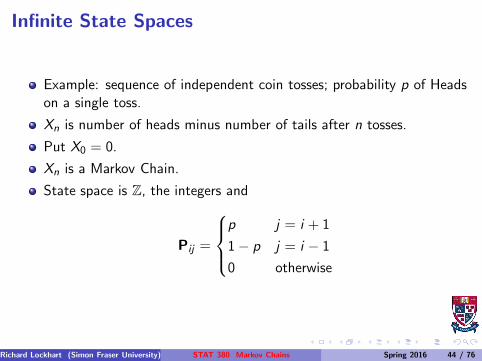
Infinite State Spaces
Example: sequence of independent coin tosses; probability p of Headson a single toss.
Xn is number of heads minus number of tails after n tosses.
Put X0 = 0.
Xn is a Markov Chain.
State space is Z, the integers and
Pij =
p j = i + 1
1− p j = i − 1
0 otherwise
Richard Lockhart (Simon Fraser University) STAT 380 Markov Chains Spring 2016 44 / 76
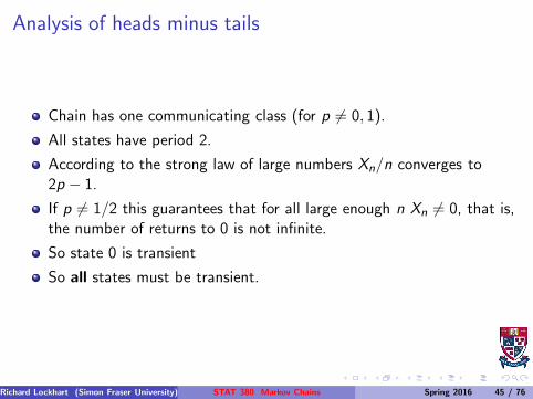
Analysis of heads minus tails
Chain has one communicating class (for p 6= 0, 1).
All states have period 2.
According to the strong law of large numbers Xn/n converges to2p − 1.
If p 6= 1/2 this guarantees that for all large enough n Xn 6= 0, that is,the number of returns to 0 is not infinite.
So state 0 is transient
So all states must be transient.
Richard Lockhart (Simon Fraser University) STAT 380 Markov Chains Spring 2016 45 / 76

Fair coin case
For p = 1/2 the situation is different.
It is a fact that
Pn00 = P(# H = # T at time n)
For n even this is the probability of exactly n/2 heads in n tosses.
Local Central Limit Theorem (normal approximation toP(−1/2 < Xn < 1/2)) (or Stirling’s approximation) shows
√2mP(Binomial(2m, 1/2) = m) → (2/π)1/2
so:∑
n
Pn00 = ∞
That is: 0 is a recurrent state.
Richard Lockhart (Simon Fraser University) STAT 380 Markov Chains Spring 2016 46 / 76
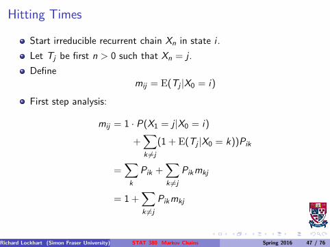
Hitting Times
Start irreducible recurrent chain Xn in state i .
Let Tj be first n > 0 such that Xn = j .
Definemij = E(Tj |X0 = i)
First step analysis:
mij = 1 · P(X1 = j |X0 = i)
+∑
k 6=j
(1 + E(Tj |X0 = k))Pik
=∑
k
Pik +∑
k 6=j
Pikmkj
= 1 +∑
k 6=j
Pikmkj
Richard Lockhart (Simon Fraser University) STAT 380 Markov Chains Spring 2016 47 / 76
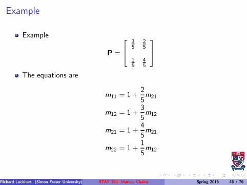
Example
Example
P =
35
25
15
45
The equations are
m11 = 1 +2
5m21
m12 = 1 +3
5m12
m21 = 1 +4
5m21
m22 = 1 +1
5m12
Richard Lockhart (Simon Fraser University) STAT 380 Markov Chains Spring 2016 48 / 76
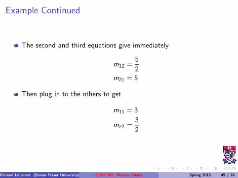
Example Continued
The second and third equations give immediately
m12 =5
2m21 = 5
Then plug in to the others to get
m11 = 3
m22 =3
2
Richard Lockhart (Simon Fraser University) STAT 380 Markov Chains Spring 2016 49 / 76

Relation to Stationary Initial Distribution
Notice stationary initial distribution is
(
1
m11,
1
m22
)
Consider fraction of time spent in state j :
1(X0 = j) + · · ·+ 1(Xn = j)
n + 1
Imagine chain starts in state i ; take expected value.
∑nr=1 P
rij + 1(i = j)
n + 1=
∑nr=0 P
rij
n + 1
If rows of Pn converge to π then fraction converges to πj ; i.e. limitingfraction of time in state j is πj .
Richard Lockhart (Simon Fraser University) STAT 380 Markov Chains Spring 2016 50 / 76

Heuristics
Heuristic: start chain in i .
Expect to return to i every mii time units.
So are in state i about once every mii time units; i.e. limiting fractionof time in state i is 1/mii .
Conclusion: for an irreducible recurrent finite state space Markovchain
πi =1
mii
.
Richard Lockhart (Simon Fraser University) STAT 380 Markov Chains Spring 2016 51 / 76
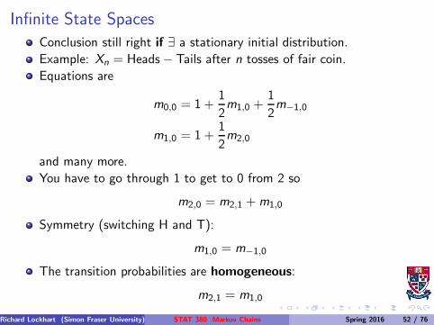
Infinite State Spaces
Conclusion still right if ∃ a stationary initial distribution.
Example: Xn = Heads− Tails after n tosses of fair coin.
Equations are
m0,0 = 1 +1
2m1,0 +
1
2m−1,0
m1,0 = 1 +1
2m2,0
and many more.
You have to go through 1 to get to 0 from 2 so
m2,0 = m2,1 +m1,0
Symmetry (switching H and T):
m1,0 = m−1,0
The transition probabilities are homogeneous:
m2,1 = m1,0
Richard Lockhart (Simon Fraser University) STAT 380 Markov Chains Spring 2016 52 / 76
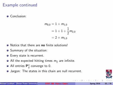
Example continued
Conclusion:
m0,0 = 1 +m1,0
= 1 + 1 +1
2m2,0
= 2 +m1,0
Notice that there are no finite solutions!
Summary of the situation:
Every state is recurrent.
All the expected hitting times mij are infinite.
All entries Pnij converge to 0.
Jargon: The states in this chain are null recurrent.
Richard Lockhart (Simon Fraser University) STAT 380 Markov Chains Spring 2016 53 / 76
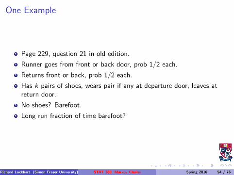
One Example
Page 229, question 21 in old edition.
Runner goes from front or back door, prob 1/2 each.
Returns front or back, prob 1/2 each.
Has k pairs of shoes, wears pair if any at departure door, leaves atreturn door.
No shoes? Barefoot.
Long run fraction of time barefoot?
Richard Lockhart (Simon Fraser University) STAT 380 Markov Chains Spring 2016 54 / 76
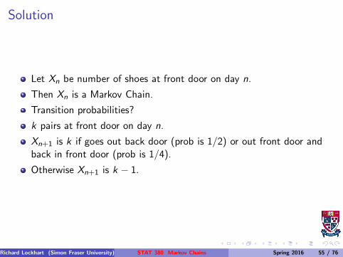
Solution
Let Xn be number of shoes at front door on day n.
Then Xn is a Markov Chain.
Transition probabilities?
k pairs at front door on day n.
Xn+1 is k if goes out back door (prob is 1/2) or out front door andback in front door (prob is 1/4).
Otherwise Xn+1 is k − 1.
Richard Lockhart (Simon Fraser University) STAT 380 Markov Chains Spring 2016 55 / 76
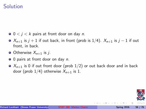
Solution
0 < j < k pairs at front door on day n.
Xn+1 is j + 1 if out back, in front (prob is 1/4). Xn+1 is j − 1 if outfront, in back.
Otherwise Xn+1 is j .
0 pairs at front door on day n.
Xn+1 is 0 if out front door (prob 1/2) or out back door and in backdoor (prob 1/4) otherwise Xn+1 is 1.
Richard Lockhart (Simon Fraser University) STAT 380 Markov Chains Spring 2016 56 / 76
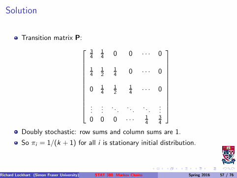
Solution
Transition matrix P:
34
14 0 0 · · · 0
14
12
14 0 · · · 0
0 14
12
14 · · · 0
......
. . .. . .
. . ....
0 0 0 · · · 14
34
Doubly stochastic: row sums and column sums are 1.
So πi = 1/(k + 1) for all i is stationary initial distribution.
Richard Lockhart (Simon Fraser University) STAT 380 Markov Chains Spring 2016 57 / 76
Solution
Solution to problem: 1 day in k + 1 no shoes at front door.
Half of those go barefoot.
Also 1 day in k + 1 all shoes at front door; go barefoot half of thesedays.
Overall go barefoot 1/(k + 1) of the time.
Richard Lockhart (Simon Fraser University) STAT 380 Markov Chains Spring 2016 58 / 76
Gambler’s Ruin
Insurance company’s reserves fluctuate: sometimes up, sometimesdown.
Ruin is event they hit 0 (company goes bankrupt).
General problem.
For given model of fluctuation compute probability of ruin eithereventually or in next k time units.
Richard Lockhart (Simon Fraser University) STAT 380 Markov Chains Spring 2016 59 / 76
Gambler’s Ruin, simple example
Simplest model: gambling on Red at Casino.
Bet $1 at a time.
Win $1 with probability p, lose $1 with probability 1− p.
Start with k dollars.
Quit playing when down to $0 or up to N.
ComputePk = P(reach N before 0|X0 = k)
Richard Lockhart (Simon Fraser University) STAT 380 Markov Chains Spring 2016 60 / 76
Gambler’s Ruin, simple example
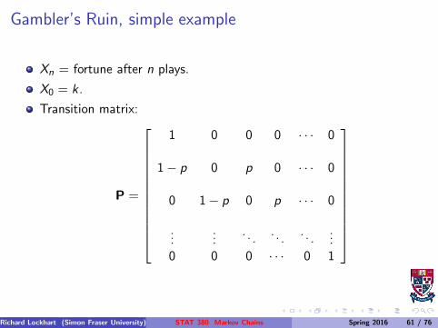
Xn = fortune after n plays.
X0 = k .
Transition matrix:
P =
1 0 0 0 · · · 0
1− p 0 p 0 · · · 0
0 1− p 0 p · · · 0
......
. . .. . .
. . ....
0 0 0 · · · 0 1
Richard Lockhart (Simon Fraser University) STAT 380 Markov Chains Spring 2016 61 / 76
Gambler’s Ruin, simple example
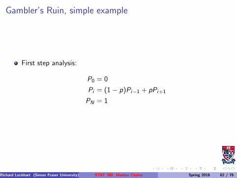
First step analysis:
P0 = 0
Pi = (1− p)Pi−1 + pPi+1
PN = 1
Richard Lockhart (Simon Fraser University) STAT 380 Markov Chains Spring 2016 62 / 76
Gambler’s Ruin, simple example
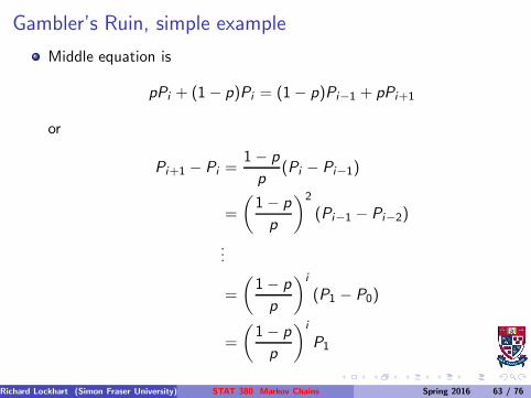
Middle equation is
pPi + (1− p)Pi = (1− p)Pi−1 + pPi+1
or
Pi+1 − Pi =1− p
p(Pi − Pi−1)
=
(
1− p
p
)2
(Pi−1 − Pi−2)
...
=
(
1− p
p
)i
(P1 − P0)
=
(
1− p
p
)i
P1
Richard Lockhart (Simon Fraser University) STAT 380 Markov Chains Spring 2016 63 / 76
Gambler’s Ruin, simple example
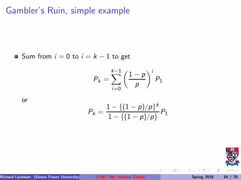
Sum from i = 0 to i = k − 1 to get
Pk =k−1∑
i=0
(
1− p
p
)i
P1
or
Pk =1− {(1− p)/p}k1− {(1− p)/p} P1
Richard Lockhart (Simon Fraser University) STAT 380 Markov Chains Spring 2016 64 / 76
Gambler’s Ruin, simple example
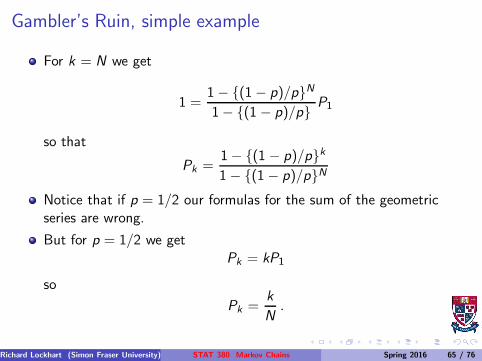
For k = N we get
1 =1− {(1− p)/p}N1− {(1 − p)/p} P1
so that
Pk =1− {(1 − p)/p}k1− {(1− p)/p}N
Notice that if p = 1/2 our formulas for the sum of the geometricseries are wrong.
But for p = 1/2 we getPk = kP1
so
Pk =k
N.
Richard Lockhart (Simon Fraser University) STAT 380 Markov Chains Spring 2016 65 / 76
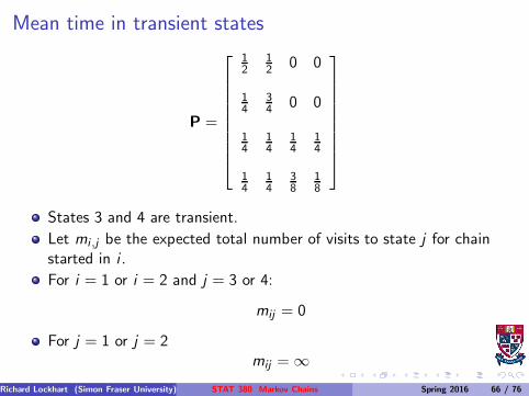
Mean time in transient states
P =
12
12 0 0
14
34 0 0
14
14
14
14
14
14
38
18
States 3 and 4 are transient.
Let mi ,j be the expected total number of visits to state j for chainstarted in i .
For i = 1 or i = 2 and j = 3 or 4:
mij = 0
For j = 1 or j = 2mij = ∞
Richard Lockhart (Simon Fraser University) STAT 380 Markov Chains Spring 2016 66 / 76
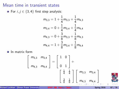
Mean time in transient states
For i , j ∈ {3, 4} first step analysis:
m3,3 = 1 +1
4m3,3 +
1
4m4,3
m3,4 = 0 +1
4m3,4 +
1
4m4,4
m4,3 = 0 +3
8m3,3 +
1
8m4,3
m4,4 = 1 +3
8m3,4 +
1
8m4,4
In matrix form
m3,3 m3,4
m4,3 m4,4
=
1 0
0 1
+
14
14
38
18
m3,3 m3,4
m4,3 m4,4
Richard Lockhart (Simon Fraser University) STAT 380 Markov Chains Spring 2016 67 / 76
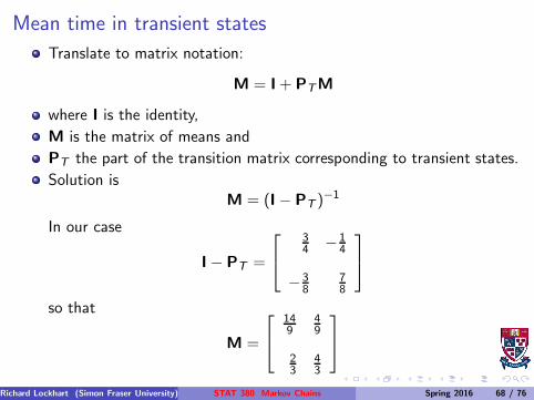
Mean time in transient states
Translate to matrix notation:
M = I+ PTM
where I is the identity,
M is the matrix of means and
PT the part of the transition matrix corresponding to transient states.
Solution isM = (I− PT )
−1
In our case
I− PT =
34 −1
4
−38
78
so that
M =
149
49
23
43
Richard Lockhart (Simon Fraser University) STAT 380 Markov Chains Spring 2016 68 / 76
Data Analysis
Imagine we have data X0, . . . ,XN which we model as coming from aMarkov Chain.
Simplest case: K states.
If we observe X0 = x0, . . . ,XN = xN how should we estimate thetransition probabilities?
Two kinds of models: parametric and ‘empirical’?
Second kind: Pij can be any probabilities subject to∑
j Pij = 1.
First kind: each Pij is function of smaller number of parameters, θ.
The θ or the Pij are parameters.
Richard Lockhart (Simon Fraser University) STAT 380 Markov Chains Spring 2016 69 / 76
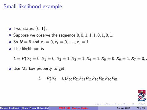
Small likelihood example
Two states {0, 1}.Suppose we observe the sequence 0, 0, 1, 1, 1, 0, 1, 0, 1.
So N = 8 and x0 = 0, x1 = 0, . . . , x8 = 1.
The likelihood is
L = P(X0 = 0,X1 = 0,X2 = 1,X3 = 1,X4 = 1,X5 = 0,X6 = 1,X7 = 0,X
Use Markov property to get
L = P(X0 = 0)P00P01P11P11P10P01P10P01
Richard Lockhart (Simon Fraser University) STAT 380 Markov Chains Spring 2016 70 / 76
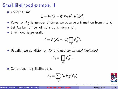
Small likelihood example, II
Collect terms:L = P(X0 = 0)P00P
301P
210P
211
Power on Pij is number of times we observe a transition from i to j .
Let Nij be number of transitions from i to j .
Likelihood is generally
L = P(X0 = x0)∏
ij
PNij
ij .
Usually: we condition on X0 and use conditional likelihood
Lc =∏
ij
PNij
ij .
Conditional log-likelihood is
ℓc =∑
ij
Nij log(Pij)
Richard Lockhart (Simon Fraser University) STAT 380 Markov Chains Spring 2016 71 / 76
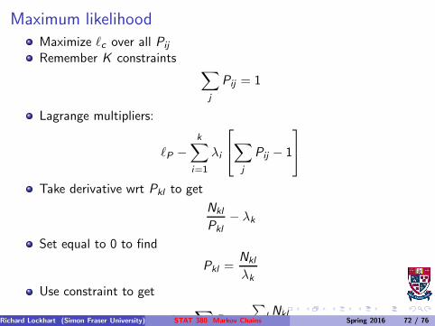
Maximum likelihood
Maximize ℓc over all Pij
Remember K constraints∑
j
Pij = 1
Lagrange multipliers:
ℓP −k
∑
i=1
λi
∑
j
Pij − 1
Take derivative wrt Pkl to get
Nkl
Pkl
− λk
Set equal to 0 to find
Pkl =Nkl
λk
Use constraint to get
1 =∑
Pkl =
∑
l Nkl
λRichard Lockhart (Simon Fraser University) STAT 380 Markov Chains Spring 2016 72 / 76
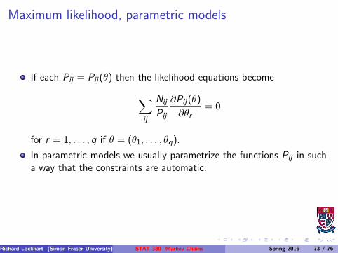
Maximum likelihood, parametric models
If each Pij = Pij(θ) then the likelihood equations become
∑
ij
Nij
Pij
∂Pij(θ)
∂θr= 0
for r = 1, . . . , q if θ = (θ1, . . . , θq).
In parametric models we usually parametrize the functions Pij in sucha way that the constraints are automatic.
Richard Lockhart (Simon Fraser University) STAT 380 Markov Chains Spring 2016 73 / 76
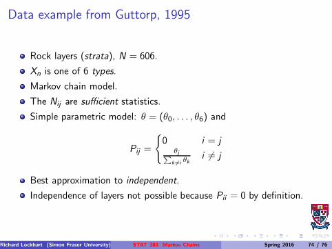
Data example from Guttorp, 1995
Rock layers (strata), N = 606.
Xn is one of 6 types.
Markov chain model.
The Nij are sufficient statistics.
Simple parametric model: θ = (θ0, . . . , θ6) and
Pij =
{
0 i = jθj∑k 6=i θk
i 6= j
Best approximation to independent.
Independence of layers not possible because Pii = 0 by definition.
Richard Lockhart (Simon Fraser University) STAT 380 Markov Chains Spring 2016 74 / 76
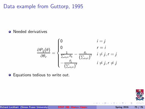
Data example from Guttorp, 1995
Needed derivatives
∂Pij(θ)
∂θr=
0 i = j
0 r = i1∑
k 6=i θk− θr
(∑
k 6=i)2 i 6= j , r = j
− θj
(∑
k 6=i)2 i 6= j , r 6= j
Equations tedious to write out.
Richard Lockhart (Simon Fraser University) STAT 380 Markov Chains Spring 2016 75 / 76
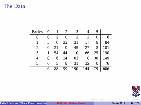
The Data
Facies 0 1 2 3 4 5
0 0 2 0 2 2 0 61 5 0 23 31 17 8 842 0 21 0 45 27 8 1013 1 54 44 0 66 25 1904 0 6 24 81 0 38 1495 0 5 8 31 32 0 76
6 88 99 190 144 79 606
Richard Lockhart (Simon Fraser University) STAT 380 Markov Chains Spring 2016 76 / 76