1

Stat 406: Algorithms for classification andprediction

Lecture 1: Introduction

Kevin Murphy

Wed 4 January, 20051

1Slides last updated on January 4, 2006

2

Outline

• Administrivia

•Machine learning: some basic definitions.

• Simple examples of regression.

• Real-world applications of regression.

• Simple examples of classification.

• Real-world applications of classification.

3

Administrivia

•Web pagehttp://www.cs.ubc.ca/∼murphyk/Teaching/Stat406 Spring06/index.html

• Please fill out the sign-up sheet.

• Labs Wed 4-5.

• The TA is Aline Tabet.

•My office hours are Fri 2-3pm LSK 308d.

• Aline’s office hours are TBA (see web).

4

Grading

• There will be weekly homework assignments worth 20%.Out on Mondays, return on Mondays (in class).

• The homeworks will often involve programming; you may want to dothis part during the lab.

• The midterm will be in late February and is worth 40%.

• The final will be in April and is worth 40%.

5

Pre-requisites

•Math: multivariate calculus, linear algebra, probability theory.

• Stats: stats 306 or CS 340 or equivalent.

• CS: some experience with programming (eg in R) is required.

6

Matlab

• There will be weekly programming assignments (as part of the lab).

•We will use matlab for programming.

•Matlab is very similar to R, but is somewhat faster and easier tolearn. Matlab is widely used in the machine learning and Bayesianstatistics community.

• Unfortunately matlab is not free (unlike R). You can buy a copy fromthe bookstore for $150, or you can use the copy installed in the labmachines.

• You will learn how to use matlab during the first few labs.

7

Textbook

• There is no official textbook. I will hand out various notes in class,including some chapters from the following unfinished/ unpublishedbooks

– Probabilistic graphical models, Michael Jordan, 2006

– Pattern recognition and machine learning, Chris Bishop, 2006

The following (already published) books are also recommended

– Elements of statistical learning, Hastie, Friedman and Tibshirani,2001. (Available from the bookstore)

– Pattern Classification, Duda, Hart, Stork, 2001 (2nd edition).

– Statistical pattern recognition, Andrew Webb, 2002.

8

Syllabus

• Since this is a new course, the syllabus is likely to change during thecourse of the semester.

• See the web page for details.

• You will get a good feeling for the class during today’s lecture.

9

Outline

• Administrivia√

•Machine learning: some basic definitions.

• Simple examples of regression.

• Real-world applications of regression.

• Simple examples of classification.

• Real-world applications of classification.

10

Learning to predict

• This class is about supervised approaches to machine learning.

• Given a training set of n = ND input-output pairs D = (~xi, ~yi)NDi=1 ,

we attempt to construct a function f which will accurately predictf (~x∗) on future, test examples ~x∗.

• Each input ~xi is a vector of p = NX features or covariates. Eachoutput ~yi is a target variable. The training data is stored in anND×NX design matrix X = [~xT

i ]. The training outputs are stored

in a ND × NY matrix Y = [~yTi ].

11

Classification vs regression

• If ~y ∈ IRNY is a continuous-valued output, this is called regres-

sion. Often we will assume NY = 1, i.e., scalar output.

• If y ∈ {1, . . . , NY } is a discrete label, this is called classifica-

tion or pattern recognition. The labels can be ordered (eg.low, medium, high) or unordered (e.g., male, female). NY is thenumber of classes. If NY = 2, this is called binary (dichotomous)classification.

12

Notation

•We will denote discrete ranges {1, . . . , N} by 1 : N .

•We will often encode categorical variables as binary vectors. eg ify ∈ {1, . . . , 3}, we will use ~y ∈ {0, 1}3, where y = 1 maps to~y = (1, 0, 0), y = 2 maps to ~y = (0, 1, 0), and y = 3 maps to~y = (0, 0, 1).

• In general, Y = j turns bit j of ~Y on, with the constraint∑NY

j=1 ~y = 1.

13

Short/fat vs tall/skinny data

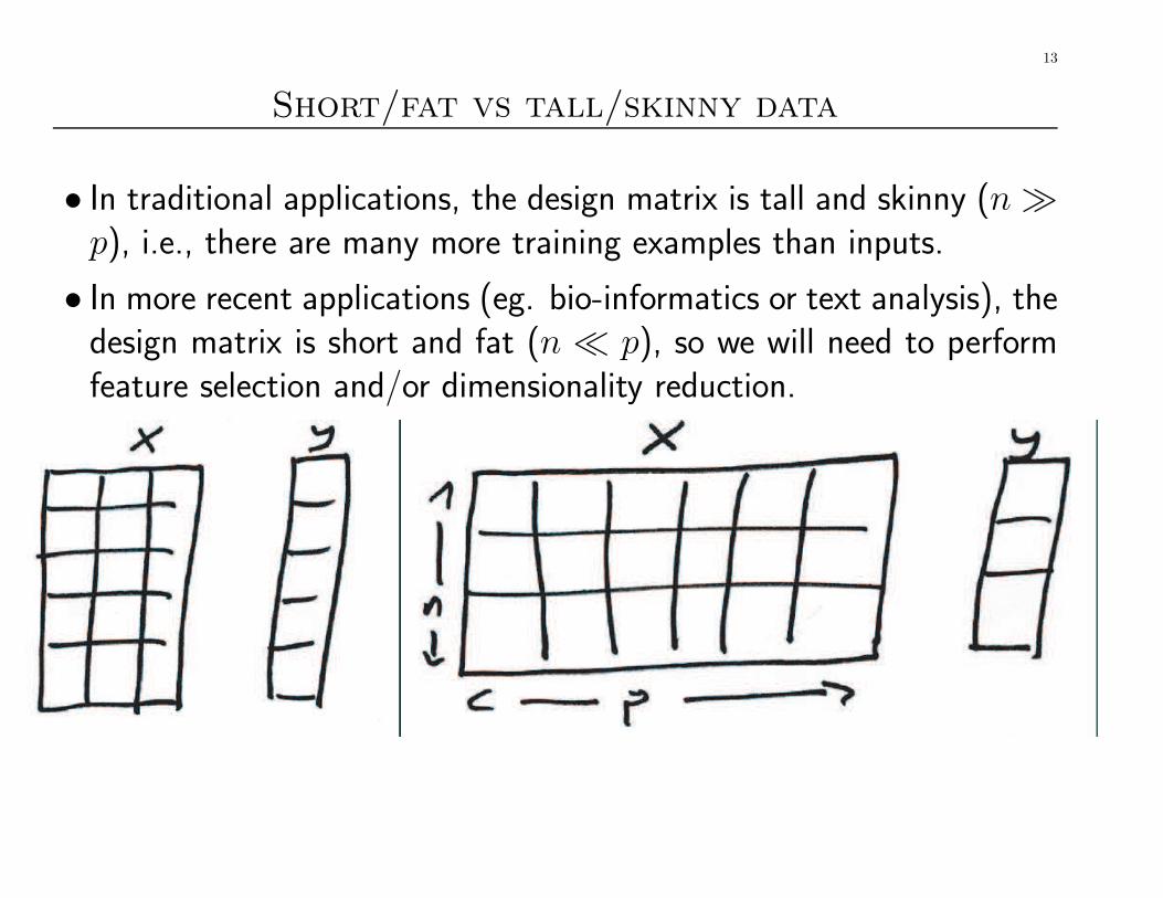
• In traditional applications, the design matrix is tall and skinny (n �p), i.e., there are many more training examples than inputs.

• In more recent applications (eg. bio-informatics or text analysis), thedesign matrix is short and fat (n � p), so we will need to performfeature selection and/or dimensionality reduction.

14

Generalization performance

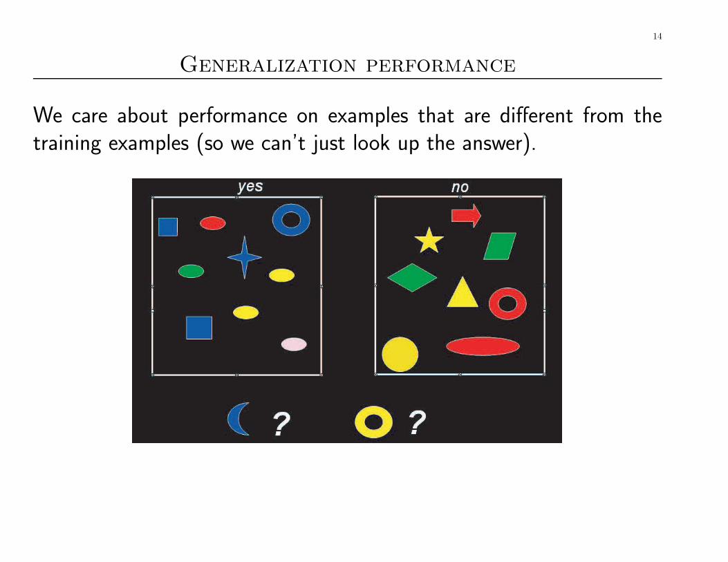
We care about performance on examples that are different from thetraining examples (so we can’t just look up the answer).

15

No free lunch theorem

• The no free lunch theorem says (roughly) that there is no singlemethod that is better at predicting across all possible data sets thanany other method.

•Different learning algorithms implicitly make different assumptionsabout the nature of the data, and if they work well, it is because theassumptions are reasonable in a particular domain.

16

Supervised vs unsupervised learning

• In supervised learning, we are given (~xi, ~yi) pairs and try to learnhow to predict ~y∗ given ~x∗.

• In unsupervised learning, we are just given ~xi vectors.

• The goal in unsupervised learning is to learn a model that “explains”the data well. There are two main kinds:

– Dimensionality reduction (eg PCA)

– Clustering (eg K-means)

17

Outline

• Administrivia√

•Machine learning: some basic definitions.√

• Simple examples of regression.

• Real-world applications of regression.

• Simple examples of classification.

• Real-world applications of classification.

18

Linear regression

The output density is a 1D Gaussian (Normal) conditional on x:

p(y|~x) = N (y; ~βT~x, σ) = N (y; β0 + β1x1 + · · · βpxp, σ)

N (y|µ, σ) =1√2πσ

exp(− 1

2σ2(y − µ)T (y − µ))

For example, y = ax1 + b is represented as ~x = (1, x1) and ~β = (b, a).

19

Polynomial regression

If we use linear regression with non-linear basis functions

p(y|x1) = N (y|βT [1, x1, x21, . . . , x

k1 ], σ)

we can produce curves like the one below.Note: In this class, we will often use ~w instead of ~β to denote theweight vector.

20

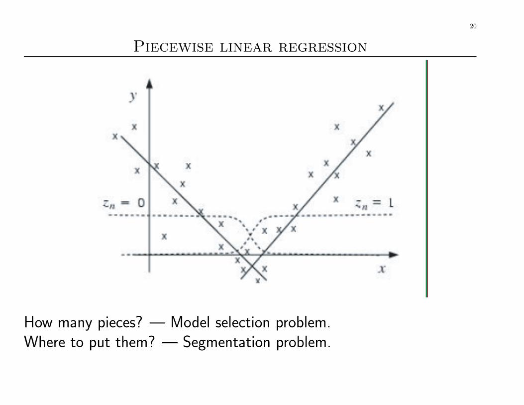
Piecewise linear regression

How many pieces? — Model selection problem.Where to put them? — Segmentation problem.

21

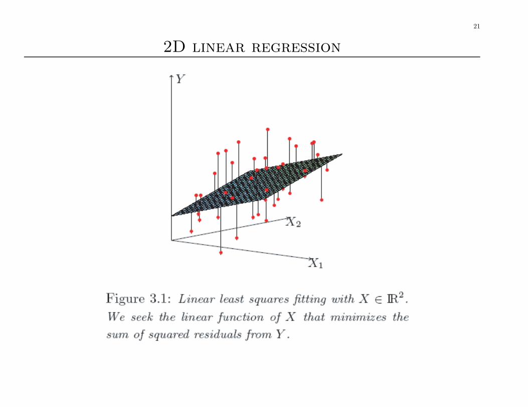
2D linear regression

22

Piecewise linear 2D regression

How many pieces? — Model selection problem.Where to put them? — Segmentation problem.

23

Outline

• Administrivia√

•Machine learning: some basic definitions.√

• Simple examples of regression.√

• Real-world applications of regression.

• Simple examples of classification.

• Real-world applications of classification.

24

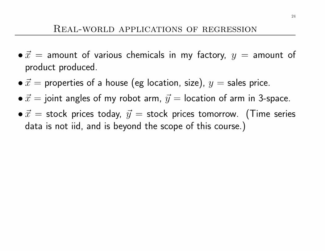
Real-world applications of regression

• ~x = amount of various chemicals in my factory, y = amount ofproduct produced.

• ~x = properties of a house (eg location, size), y = sales price.

• ~x = joint angles of my robot arm, ~y = location of arm in 3-space.

• ~x = stock prices today, ~y = stock prices tomorrow. (Time seriesdata is not iid, and is beyond the scope of this course.)

25

Outline

• Administrivia√

•Machine learning: some basic definitions.√

• Simple examples of regression.√

• Real-world applications of regression.√

• Simple examples of classification.

• Real-world applications of classification.

26

Linearly separable 2D data

2D inputs ~xi ∈ IR2, binary outputs y ∈ {0, 1}.The line is called a decision boundary.Points to the right are classified as y = 1, points to the left as y = 0.

27

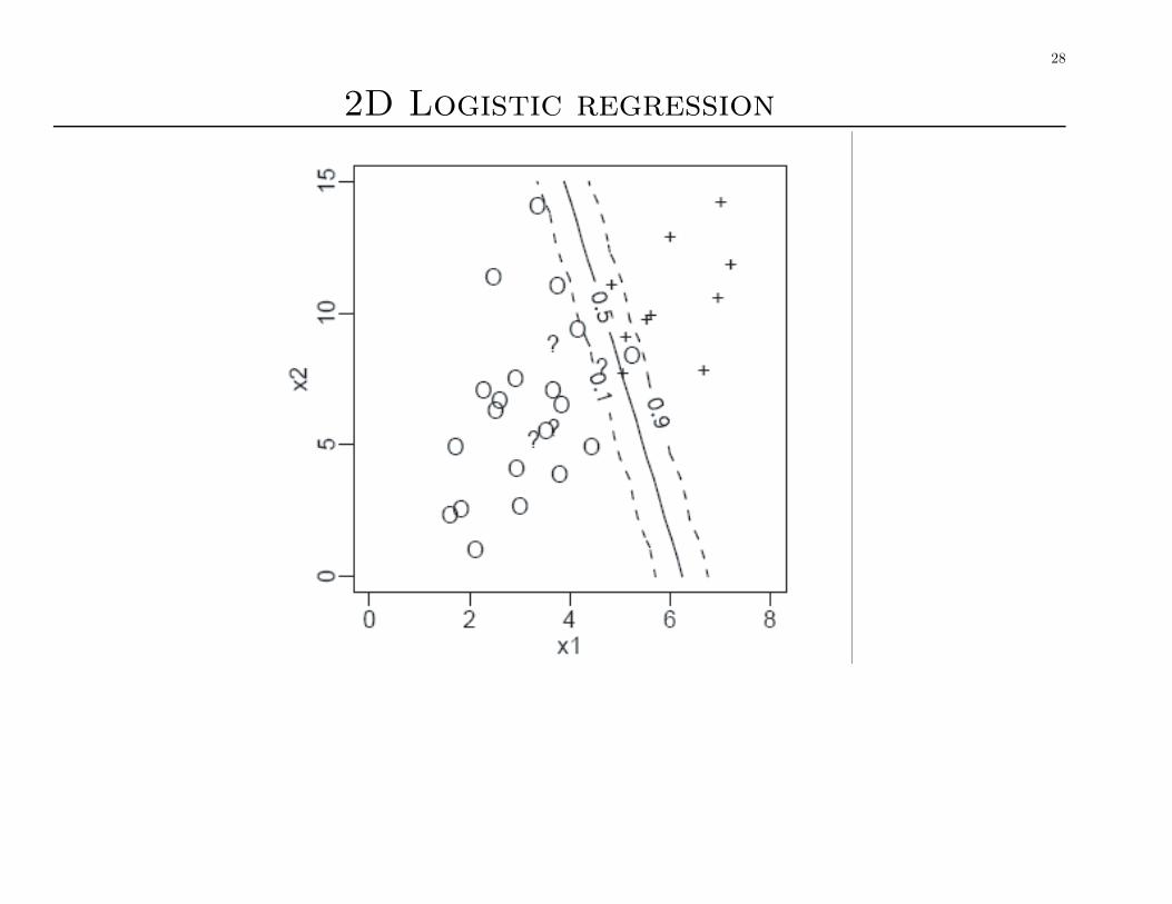
Logistic regression

• A simple approach to binary classification is logistic regression (brieflystudied in 306).

• The output density is Bernoulli conditional on x:

p(y|x) = π(x)y (1 − π(x))1−y

where y ∈ {0, 1} and

π(x) = σ(~wT [1, x1, x2])

where

σ(u) =1

1 + e−u

is the sigmoid (logistic) function that maps IR to [0, 1]. Hence

P (Y = 1|~x) =1

1 + e−w0+w1x1+w2x2

where w0 is the bias (offset) term corresponding to the dummy col-umn of 1s added to the design matrix.

28

2D Logistic regression

29

Non-linearly separable 2D data

In 306, this is called “checkerboard” data.In machine learning, this is called the “xor” problem.The “true” function is y = x1 ⊕ x2.The decision boundary is non-linear.

30

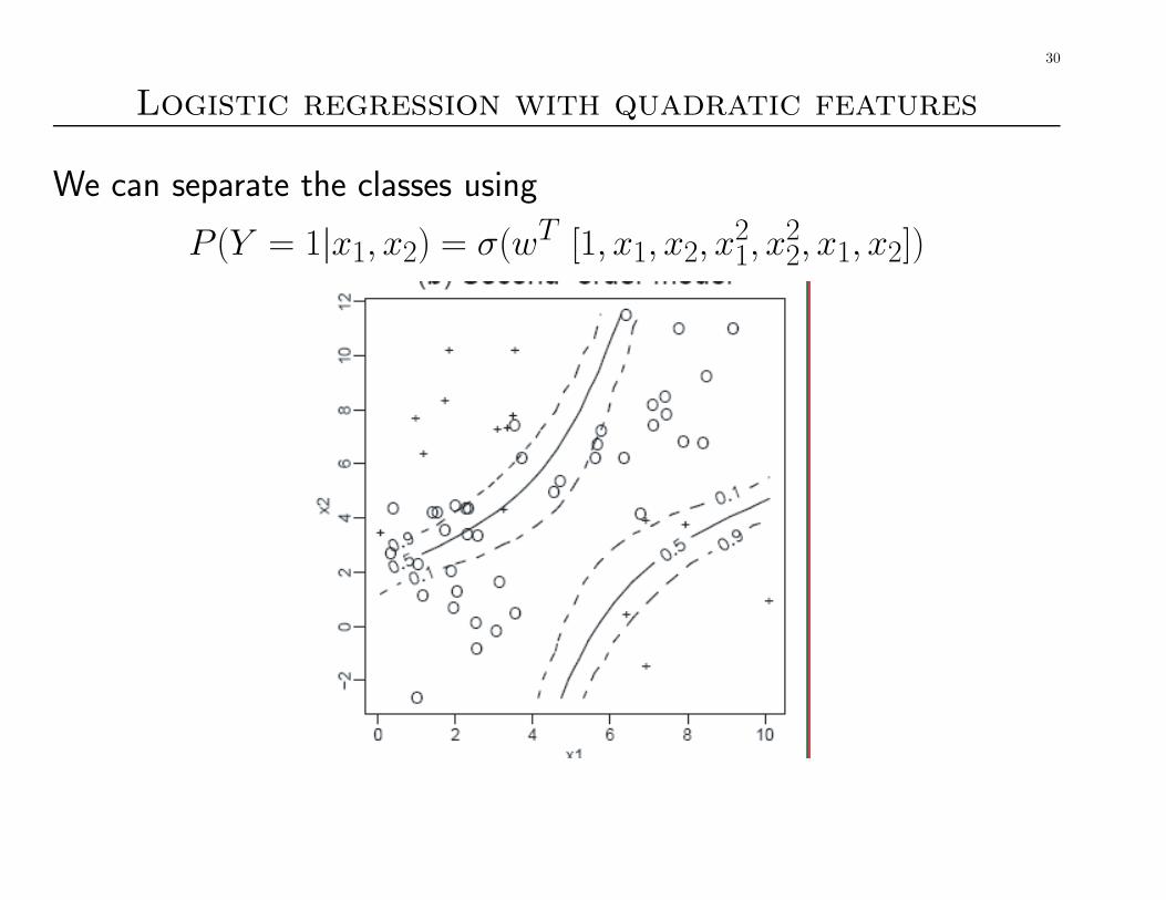
Logistic regression with quadratic features

We can separate the classes using

P (Y = 1|x1, x2) = σ(wT [1, x1, x2, x21, x

22, x1, x2])

31

Outline

• Administrivia√

•Machine learning: some basic definitions.√

• Simple examples of regression.√

• Real-world applications of regression.√

• Simple examples of classification.√

• Real-world applications of classification.

32

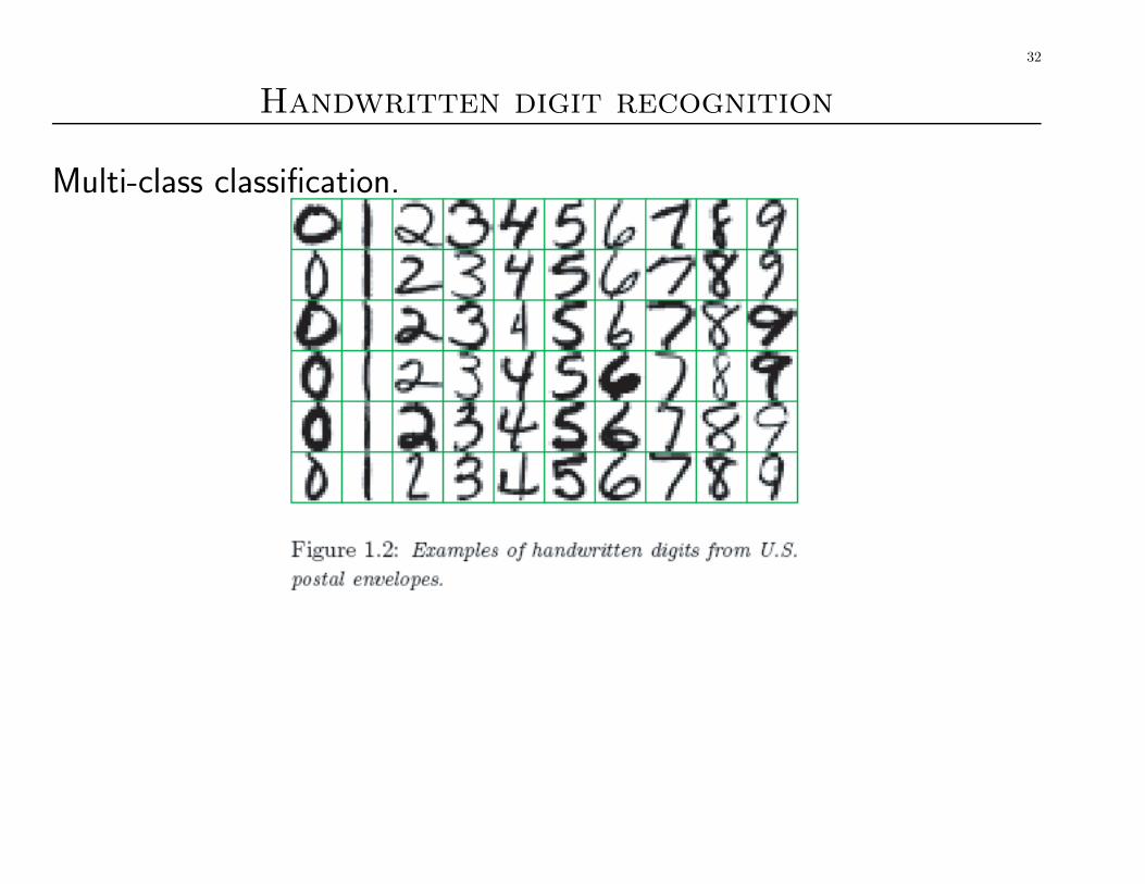
Handwritten digit recognition

Multi-class classification.

33

Gene microarray expression data

Rows = examples, columns = features (genes).Short, fat data (p � N).Might need to perform feature selection.

34

Other examples of classification

• Email spam filtering (spam vs not spam)

•Detecting credit card fraud (fraudulent or legitimate)

• Face detection in images (face or background)

•Web page classification (sports vs politics vs entertainment etc)

• Steering an autonomous car across the US (turn left, right, or gostraight)