STAT 430 (Fall 2017): Tutorial 8

Balanced Incomplete Block Design

Luyao Lin

November 7th/9th, 2017

Department Statistics and Actuarial Science, Simon Fraser University

Block Design

• Complete

• Random Complete Block Design

• Incomplete Block Design

• Balanced Incomplete Block Design (BIBD)

• Latin Square Design

1

Incomplete Block Design

• Why we need it?

• Advantage of it?

• Disadvantage of it?

• How to do it?

2

Why ‘Incomplete’ Block Design? (Motivation)

Block sizes

• Complete Block Design, every block can hold every treatment level

at least once.

• Incomplete Block Design, the block size is less than the treatment

level.

Suppose we have 4 different treatment levels, but each

block can only have 2 experiment units.

• Balanced Incomplete Block Design (BIBD)

3

Balanced Incomplete Block Design (BIBD)

• v treatment level

• r : each treatment appears in r blocks

• b blocks; b > r

• k each block size (# of units each block can have)

• λ: each pair of the treatment appears together in λ blocks (why we

care about this ?)

• total # of units: bk or vr

4

Balanced Incomplete Block Design (BIBD)

• v treatment level

• r each treatment appears in r

blocks

• b blocks; b > r

• k each block size (# of units

each block can have)

• λ: each pair of the treatment

appears together in λ blocks

• total # of units: bk or vr

5

Properties of BIBD

Requirements:

(i) Each treatment must appear the same number of times in the

design: vr = bk

(ii) each pair of treatments appears together in λ blocks

r(k − 1) = λ(v − 1)

Advantage:

• all treatment contrasts estimable

• all pairwise comparisons are estimated with the same variance

• tends to give the shortest CIs for contrasts

Disadvantage: for certain value of b, k , v , r , BIBD might not exist. If

b = v = 8, r = k = 3, λ =?

6

r(k − 1) = λ(v − 1)

• for treatment say A, it appears

in r blocks

• within those r blocks, there are

in total r(k − 1) treatments

other than A itself

• on the other hand, we have

v − 1 other treatment levels

• A is supposed to appear with

each of them in λ blocks

• so that λ(v − 1) = r(k − 1)

• v treatment level

• r each treatment appears in r

blocks

• b blocks; b > r

• k each block size (# of units

each block can have)

• λ: each pair of the treatment

appears together in λ blocks

• total # of units: bk or vr

7

Revisit the example

8

How to analyze BIBD?

Yhi = µ+ θh + τi + εij

• εi.i.d.∼ N(0, σ2)

• h = 1, . . . , b, i = 1, . . . , v

• (h, i) in the design

•∑τi = 0

∑θh = 0

Assumptions for Yhi ∼ N(µ+ θh + τi , σ2)

• normality

• equal variance

• independence

• no interaction effect (hard to verify)

9

Parameter Estimation: least square

• unadjusted estimate: τi = Y.i

E (Y.1 − Y.2) = τ1 − τ2 +1

7

( 7∑h=4

θh −11∑h=8

θh

)6= τ1 − τ2

• adjusted estimate (section 11.3.2)

r(k − 1)τi − λ∑p 6=i

τp = kQi

Qi = Ti −1

k

∑h

nhiBh

(Intra-block equations)

• Ti is the total of response on treatment i

• Bh is the total of response in block h

• nhi is 1 if i is in block h or 0 otherwise

10

adjusted estimate (section 11.3.2)

r(k − 1)τi − λ∑p 6=i

τp = kQi

along with∑

i τi = 0

r(k − 1)τi + λτi = kQi

τi =kQi

r(k − 1) + λ=

kQi

λv=

kTi −∑

h nhiBh

λv

because λ(v − 1) = r(k − 1)

τi =kQi

λv

11

Other Parameters Estimate

Yhi = µ+ θh + τi + εij

• τi = kQi

λv

• µ = Gbk ; G is the grand total

•

θh =Bh

k− G

bk−∑v

i=1 nhi τik

• σ2 = mse = SSEbk−b−v+1

12

ANOVA table

bk − b − v − 1 SSE =b∑

h=1

v∑i=1

nhi e2hi =

b∑h=1

v∑i=1

(yhi − µ− θh − τi )2

=b∑

h=1

v∑i=1

y 2hi −

1

k

b∑h=1

B2h −

v∑i=1

Qi τ2i

bk − 1 SStot =b∑

h=1

v∑i=1

y 2hi −

1

bkG 2

b − 1 SSθ =1

k

b∑h=1

B2h − 1

bkG 2

v − 1 SSTadj =v∑

i=1

Qi τ2i

F0 =MsTadj

MSE

13

CI for the contrasts

• τi = kλvQi

• Var(Qi ) = σ2

• Var(∑

ci τi ) =∑

c2ikλv σ

2

• CI for∑

ci τi : (k

λv

∑ciQi ± w

√∑c2i

k

λvσ2

)• wB = ttk−b−v+1,α/2m,wT = qv ,bk−b−v+1,α/

√2

Section 11.4.2 has a good example for BIBD page 355

14

The Latin Square Design

15

Big picture

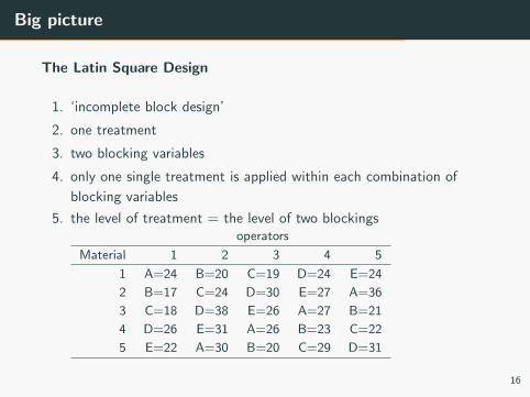
The Latin Square Design

1. ‘incomplete block design’

2. one treatment

3. two blocking variables

4. only one single treatment is applied within each combination of

blocking variables

5. the level of treatment = the level of two blockingsoperators

Material 1 2 3 4 5

1 A=24 B=20 C=19 D=24 E=24

2 B=17 C=24 D=30 E=27 A=36

3 C=18 D=38 E=26 A=27 B=21

4 D=26 E=31 A=26 B=23 C=22

5 E=22 A=30 B=20 C=29 D=31

16

why use a Latin Square?

1. impossible to use each treatment level for the same combination of

blocking

2. for example, consider an experiment with four diets, each to be

given to four cows in succession

3. each cow can only be given a single diet during a single time period.

4. one block factor is the cow, the other block factor is the time or the

ordertime

cow 1 2 3 4

1 C A D B

2 A B C D

3 D C B A

4 B D A C

5. Latin square is not unique; as long as each letter (treatment)

appears in each row and column exactly once.

17

R function

latin=

function (n, nrand = 20)

{

x = matrix(LETTERS [1:n], n, n)

x = t(x)

for (i in 2:n) x[i, ] = x[i, c(i:n, 1:(i -

1))]

if (nrand > 0) {

for (i in 1:nrand) {

x = x[sample(n), ]

x = x[, sample(n)]

}

}

x

}

latin (5)

[,1] [,2] [,3] [,4] [,5]

[1,] "E" "D" "C" "B" "A"

[2,] "D" "C" "B" "A" "E"

[3,] "C" "B" "A" "E" "D"

[4,] "A" "E" "D" "C" "B"

[5,] "B" "A" "E" "D" "C"

latin (4)

[,1] [,2] [,3] [,4]

[1,] "A" "C" "B" "D"

[2,] "B" "D" "C" "A"

[3,] "D" "B" "A" "C"

[4,] "C" "A" "D" "B"

18

Model

yijk = µ+ αi + τj + βk + εijk

• yijk : ith row, kth col, jth treatment; i , j , k = 1, 2, . . . , p

• µ overall mean, αi ith row effect; τj jth treatment effect; βk kth

column effect ∑αi =

∑τj =

∑βk = 0

• εijk ∼ iid N(0, σ2)

• N = p2

SST =SSrows + SScol + SStreatment + SSE

p2 − 1 =p − 1 + p − 1 + p − 1 + (p − 2)(p − 1)

19

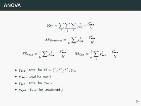
ANOVA

SST =∑i

∑j

∑k

y2ijk −

y2•••N

SSTreatment =1

p

∑j

y2•j• −

y2•••N

SSRows =1

p

∑i

y2i•• −

y2•••N

SSCols =1

p

∑k

y2••k −

y2•••N

• y••• : total for all =∑

i

∑j

∑k yijk

• yi•• : total for row i

• y••k : total for row k

• y•j•k : total for treatment j

20

Model Continued

1. Hull hypothesis:

τ1 = τ2 = . . . = τp = 0

2. Alternative hypothsis: at least one of them is not zero

3. Test statistics:

F =MStreatment

MSE=

SStreatmet/(p − 1)

SSE/(p − 2)(p − 1)

4. residuals are given as

eijk = yijk − yijk = yijk − y i•• − y•j• − y••k + 2y•••

21