Embed Size (px)
Citation preview
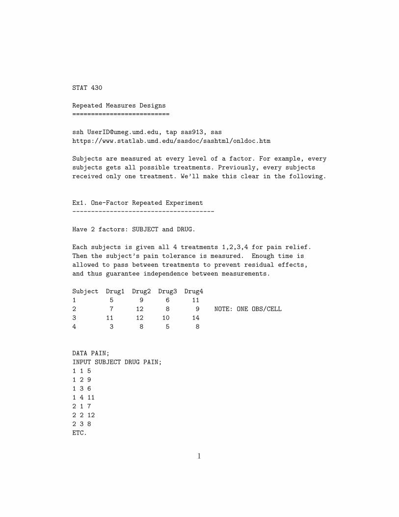
STAT 430
Repeated Measures Designs
==========================
ssh [email protected], tap sas913, sas
https://www.statlab.umd.edu/sasdoc/sashtml/onldoc.htm
Subjects are measured at every level of a factor. For example, every
subjects gets all possible treatments. Previously, every subjects
received only one treatment. We’ll make this clear in the following.
Ex1. One-Factor Repeated Experiment
--------------------------------------
Have 2 factors: SUBJECT and DRUG.
Each subjects is given all 4 treatments 1,2,3,4 for pain relief.
Then the subject’s pain tolerance is measured. Enough time is
allowed to pass between treatments to prevent residual effects,
and thus guarantee independence between measurements.
Subject Drug1 Drug2 Drug3 Drug4
1 5 9 6 11
2 7 12 8 9 NOTE: ONE OBS/CELL
3 11 12 10 14
4 3 8 5 8
DATA PAIN;
INPUT SUBJECT DRUG PAIN;
1 1 5
1 2 9
1 3 6
1 4 11
2 1 7
2 2 12
2 3 8
ETC.
1
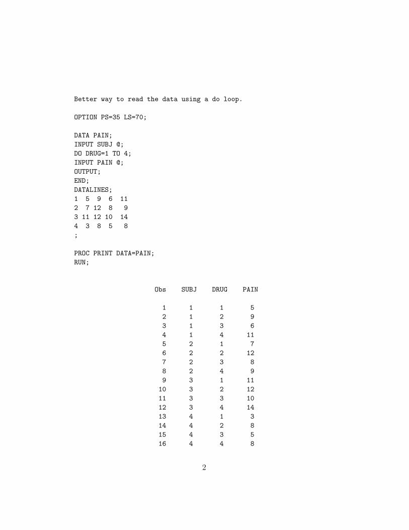
Better way to read the data using a do loop.
OPTION PS=35 LS=70;
DATA PAIN;
INPUT SUBJ @;
DO DRUG=1 TO 4;
INPUT PAIN @;
OUTPUT;
END;
DATALINES;
1 5 9 6 11
2 7 12 8 9
3 11 12 10 14
4 3 8 5 8
;
PROC PRINT DATA=PAIN;
RUN;
Obs SUBJ DRUG PAIN
1 1 1 5
2 1 2 9
3 1 3 6
4 1 4 11
5 2 1 7
6 2 2 12
7 2 3 8
8 2 4 9
9 3 1 11
10 3 2 12
11 3 3 10
12 3 4 14
13 4 1 3
14 4 2 8
15 4 3 5
16 4 4 8
2
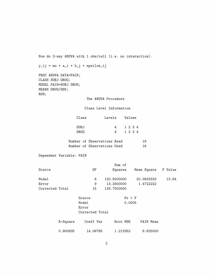
Now do 2-way ANOVA with 1 obs/cell (i.e. no interaction).
y_ij = mu + a_i + b_j + epsilon_ij
PROC ANOVA DATA=PAIN;
CLASS SUBJ DRUG;
MODEL PAIN=SUBJ DRUG;
MEANS DRUG/SNK;
RUN;
The ANOVA Procedure
Class Level Information
Class Levels Values
SUBJ 4 1 2 3 4
DRUG 4 1 2 3 4
Number of Observations Read 16
Number of Observations Used 16
Dependent Variable: PAIN
Sum of
Source DF Squares Mean Square F Value
Model 6 120.5000000 20.0833333 13.64
Error 9 13.2500000 1.4722222
Corrected Total 15 133.7500000
Source Pr > F
Model 0.0005
Error
Corrected Total
R-Square Coeff Var Root MSE PAIN Mean
0.900935 14.06785 1.213352 8.625000
3
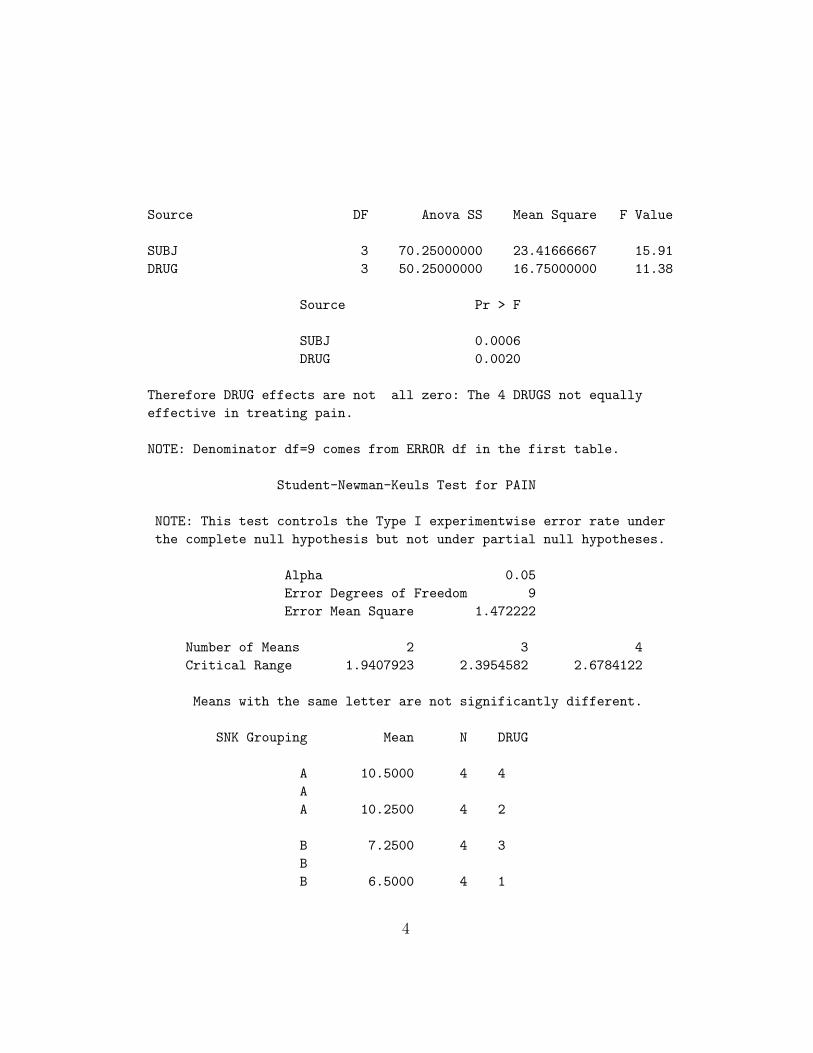
Source DF Anova SS Mean Square F Value
SUBJ 3 70.25000000 23.41666667 15.91
DRUG 3 50.25000000 16.75000000 11.38
Source Pr > F
SUBJ 0.0006
DRUG 0.0020
Therefore DRUG effects are not all zero: The 4 DRUGS not equally
effective in treating pain.
NOTE: Denominator df=9 comes from ERROR df in the first table.
Student-Newman-Keuls Test for PAIN
NOTE: This test controls the Type I experimentwise error rate under
the complete null hypothesis but not under partial null hypotheses.
Alpha 0.05
Error Degrees of Freedom 9
Error Mean Square 1.472222
Number of Means 2 3 4
Critical Range 1.9407923 2.3954582 2.6784122
Means with the same letter are not significantly different.
SNK Grouping Mean N DRUG
A 10.5000 4 4
A
A 10.2500 4 2
B 7.2500 4 3
B
B 6.5000 4 1
4
We see that DRUGS 4,2 and 3,1 are "same". Assuming a higher mean
indicates greater pain, DRUGS 1,3 more effective in treating pain.
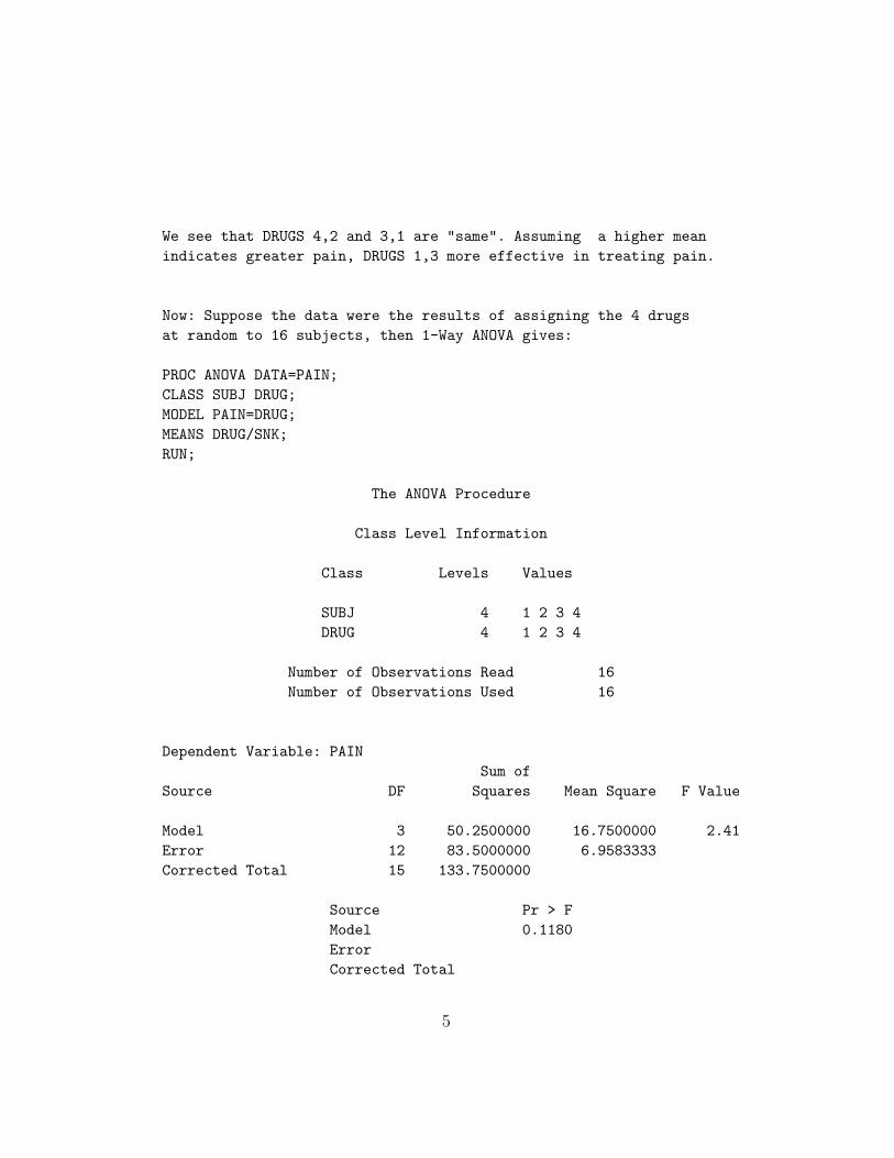
Now: Suppose the data were the results of assigning the 4 drugs
at random to 16 subjects, then 1-Way ANOVA gives:
PROC ANOVA DATA=PAIN;
CLASS SUBJ DRUG;
MODEL PAIN=DRUG;
MEANS DRUG/SNK;
RUN;
The ANOVA Procedure
Class Level Information
Class Levels Values
SUBJ 4 1 2 3 4
DRUG 4 1 2 3 4
Number of Observations Read 16
Number of Observations Used 16
Dependent Variable: PAIN
Sum of
Source DF Squares Mean Square F Value
Model 3 50.2500000 16.7500000 2.41
Error 12 83.5000000 6.9583333
Corrected Total 15 133.7500000
Source Pr > F
Model 0.1180
Error
Corrected Total
5

R-Square Coeff Var Root MSE PAIN Mean
0.375701 30.58395 2.637865 8.625000
Source DF Anova SS Mean Square F Value
DRUG 3 50.25000000 16.75000000 2.41
Source Pr > F
DRUG 0.1180
Student-Newman-Keuls Test for PAIN
NOTE: This test controls the Type I experimentwise error rate under
the complete null hypothesis but not under partial null hypotheses.
Alpha 0.05
Error Degrees of Freedom 12
Error Mean Square 6.958333
Number of Means 2 3 4
Critical Range 4.0640501 4.9760399 5.5375686
Means with the same letter are not significantly different.
SNK Grouping Mean N DRUG
A 10.500 4 4
A
A 10.250 4 2
A
A 7.250 4 3
A
A 6.500 4 1
6

We see: Before with only 4 subjects, the ERROR SS was only 13.25
with df=9, and the drugs effects were significant. But now with 16
subjects, the ERROR SS absorbed the SUBJ SS 70.25 and is equal to
13.25 + 70.25 = 83.5 with df=12, and the drug effects are not significant.
We see: Controlling for between-subject variability reduces the error
SS, and allows us to identify small treatment differences with
relatively fewer subjects.
Now: use REPEATED option
-------------------------
Data must have the form: SUBJ PAIN1 PAIN2 PAIN3 PAIN4,
where PAIN1-PAIN4 are the dependent obs from each drug.
Notice: The reference to the DRUG factor is through its levels.
DATA REPEAT1;
INPUT SUBJ PAIN1-PAIN4;
DATALINES;
1 5 9 6 11
2 7 12 8 9
3 11 12 10 14
4 3 8 5 8
;
PROC PRINT DATA=REPEAT1;
ID SUBJ;
RUN;
SUBJ PAIN1 PAIN2 PAIN3 PAIN4
1 5 9 6 11
2 7 12 8 9
3 11 12 10 14
4 3 8 5 8
7
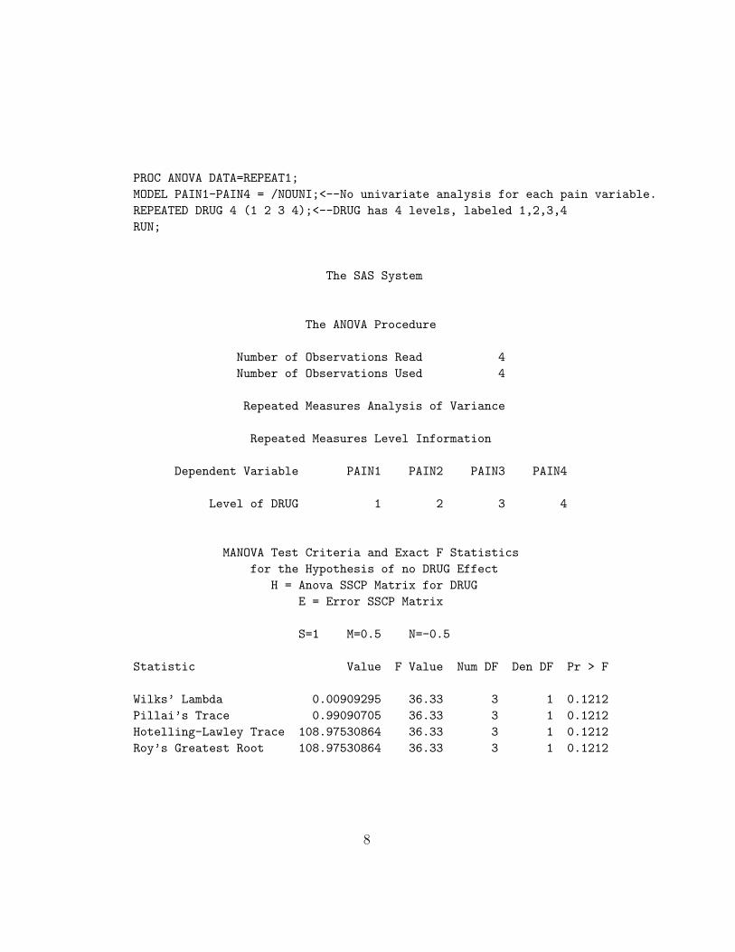
PROC ANOVA DATA=REPEAT1;
MODEL PAIN1-PAIN4 = /NOUNI;<--No univariate analysis for each pain variable.
REPEATED DRUG 4 (1 2 3 4);<--DRUG has 4 levels, labeled 1,2,3,4
RUN;
The SAS System
The ANOVA Procedure
Number of Observations Read 4
Number of Observations Used 4
Repeated Measures Analysis of Variance
Repeated Measures Level Information
Dependent Variable PAIN1 PAIN2 PAIN3 PAIN4
Level of DRUG 1 2 3 4
MANOVA Test Criteria and Exact F Statistics
for the Hypothesis of no DRUG Effect
H = Anova SSCP Matrix for DRUG
E = Error SSCP Matrix
S=1 M=0.5 N=-0.5
Statistic Value F Value Num DF Den DF Pr > F
Wilks’ Lambda 0.00909295 36.33 3 1 0.1212
Pillai’s Trace 0.99090705 36.33 3 1 0.1212
Hotelling-Lawley Trace 108.97530864 36.33 3 1 0.1212
Roy’s Greatest Root 108.97530864 36.33 3 1 0.1212
8
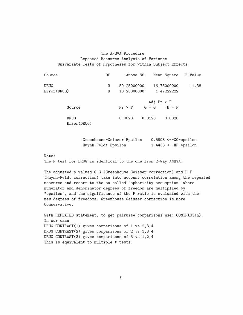
The ANOVA Procedure
Repeated Measures Analysis of Variance
Univariate Tests of Hypotheses for Within Subject Effects
Source DF Anova SS Mean Square F Value
DRUG 3 50.25000000 16.75000000 11.38
Error(DRUG) 9 13.25000000 1.47222222
Adj Pr > F
Source Pr > F G - G H - F
DRUG 0.0020 0.0123 0.0020
Error(DRUG)
Greenhouse-Geisser Epsilon 0.5998 <--GG-epsilon
Huynh-Feldt Epsilon 1.4433 <--HF-epsilon
Note:
The F test for DRUG is identical to the one from 2-Way ANOVA.
The adjusted p-valued G-G (Greenhouse-Geisser correction) and H-F
(Huynh-Feldt correction) take into account correlation among the repeated
measures and resort to the so called "sphericity assumption" where
numerator and denominator degrees of freedom are multiplied by
"epsilon", and the significance of the F ratio is evaluated with the
new degrees of freedoms. Greenhouse-Geisser correction is more
Conservative.
With REPEATED statement, to get pairwise comparisons use: CONTRAST(n).
In our case
DRUG CONTRAST(1) gives comparisons of 1 vs 2,3,4
DRUG CONTRAST(2) gives comparisons of 2 vs 1,3,4
DRUG CONTRAST(3) gives comparisons of 3 vs 1,2,4
This is equivalent to multiple t-tests.
9
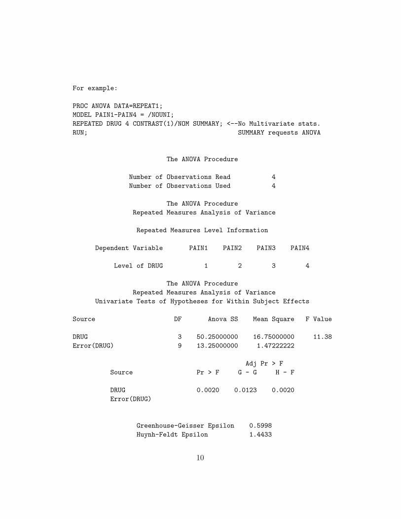
For example:
PROC ANOVA DATA=REPEAT1;
MODEL PAIN1-PAIN4 = /NOUNI;
REPEATED DRUG 4 CONTRAST(1)/NOM SUMMARY; <--No Multivariate stats.
RUN; SUMMARY requests ANOVA
The ANOVA Procedure
Number of Observations Read 4
Number of Observations Used 4
The ANOVA Procedure
Repeated Measures Analysis of Variance
Repeated Measures Level Information
Dependent Variable PAIN1 PAIN2 PAIN3 PAIN4
Level of DRUG 1 2 3 4
The ANOVA Procedure
Repeated Measures Analysis of Variance
Univariate Tests of Hypotheses for Within Subject Effects
Source DF Anova SS Mean Square F Value
DRUG 3 50.25000000 16.75000000 11.38
Error(DRUG) 9 13.25000000 1.47222222
Adj Pr > F
Source Pr > F G - G H - F
DRUG 0.0020 0.0123 0.0020
Error(DRUG)
Greenhouse-Geisser Epsilon 0.5998
Huynh-Feldt Epsilon 1.4433
10
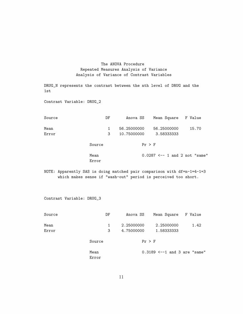
The ANOVA Procedure
Repeated Measures Analysis of Variance
Analysis of Variance of Contrast Variables
DRUG_N represents the contrast between the nth level of DRUG and the
1st
Contrast Variable: DRUG_2
Source DF Anova SS Mean Square F Value
Mean 1 56.25000000 56.25000000 15.70
Error 3 10.75000000 3.58333333
Source Pr > F
Mean 0.0287 <-- 1 and 2 not "same"
Error
NOTE: Apparently SAS is doing matched pair comparison with df=n-1=4-1=3
which makes sense if "wash-out" period is perceived too short.
Contrast Variable: DRUG_3
Source DF Anova SS Mean Square F Value
Mean 1 2.25000000 2.25000000 1.42
Error 3 4.75000000 1.58333333
Source Pr > F
Mean 0.3189 <--1 and 3 are "same"
Error
11
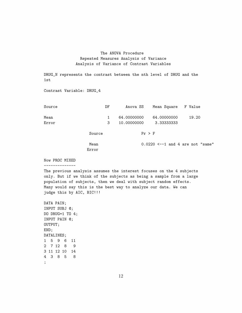
The ANOVA Procedure
Repeated Measures Analysis of Variance
Analysis of Variance of Contrast Variables
DRUG_N represents the contrast between the nth level of DRUG and the
1st
Contrast Variable: DRUG_4
Source DF Anova SS Mean Square F Value
Mean 1 64.00000000 64.00000000 19.20
Error 3 10.00000000 3.33333333
Source Pr > F
Mean 0.0220 <--1 and 4 are not "same"
Error
Now PROC MIXED
--------------
The previous analysis assumes the interest focuses on the 4 subjects
only. But if we think of the subjects as being a sample from a large
population of subjects, then we deal with subject random effects.
Many would say this is the best way to analyze our data. We can
judge this by AIC, BIC!!!
DATA PAIN;
INPUT SUBJ @;
DO DRUG=1 TO 4;
INPUT PAIN @;
OUTPUT;
END;
DATALINES;
1 5 9 6 11
2 7 12 8 9
3 11 12 10 14
4 3 8 5 8
;
12
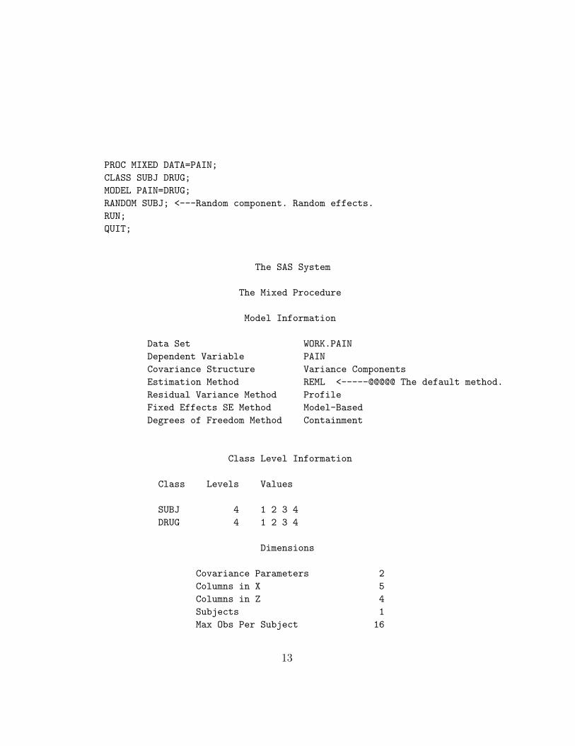
PROC MIXED DATA=PAIN;
CLASS SUBJ DRUG;
MODEL PAIN=DRUG;
RANDOM SUBJ; <---Random component. Random effects.
RUN;
QUIT;
The SAS System
The Mixed Procedure
Model Information
Data Set WORK.PAIN
Dependent Variable PAIN
Covariance Structure Variance Components
Estimation Method REML <-----@@@@@ The default method.
Residual Variance Method Profile
Fixed Effects SE Method Model-Based
Degrees of Freedom Method Containment
Class Level Information
Class Levels Values
SUBJ 4 1 2 3 4
DRUG 4 1 2 3 4
Dimensions
Covariance Parameters 2
Columns in X 5
Columns in Z 4
Subjects 1
Max Obs Per Subject 16
13
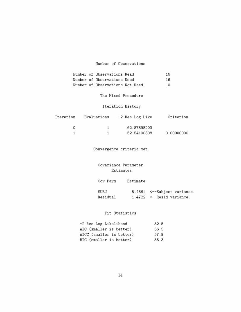
Number of Observations
Number of Observations Read 16
Number of Observations Used 16
Number of Observations Not Used 0
The Mixed Procedure
Iteration History
Iteration Evaluations -2 Res Log Like Criterion
0 1 62.87898203
1 1 52.54100308 0.00000000
Convergence criteria met.
Covariance Parameter
Estimates
Cov Parm Estimate
SUBJ 5.4861 <--Subject variance.
Residual 1.4722 <--Resid variance.
Fit Statistics
-2 Res Log Likelihood 52.5
AIC (smaller is better) 56.5
AICC (smaller is better) 57.9
BIC (smaller is better) 55.3
14

Type 3 Tests of Fixed Effects
Num Den
Effect DF DF F Value Pr > F
DRUG 3 9 11.38 0.0020 <--Same as brfore
If we use fixed effects as in two-way ANOVA as before we get better
AIC and BIC(!!!) as we see next.
PROC MIXED DATA=PAIN;
CLASS SUBJ DRUG;
MODEL PAIN=SUBJ DRUG; <--No RANDOM component!!!
RUN;
QUIT;
The Mixed Procedure
Model Information
Data Set WORK.PAIN
Dependent Variable PAIN
Covariance Structure Diagonal
Estimation Method REML <-----@@@@@
Residual Variance Method Profile
Fixed Effects SE Method Model-Based
Degrees of Freedom Method Residual
Class Level Information
Class Levels Values
SUBJ 4 1 2 3 4
DRUG 4 1 2 3 4
15
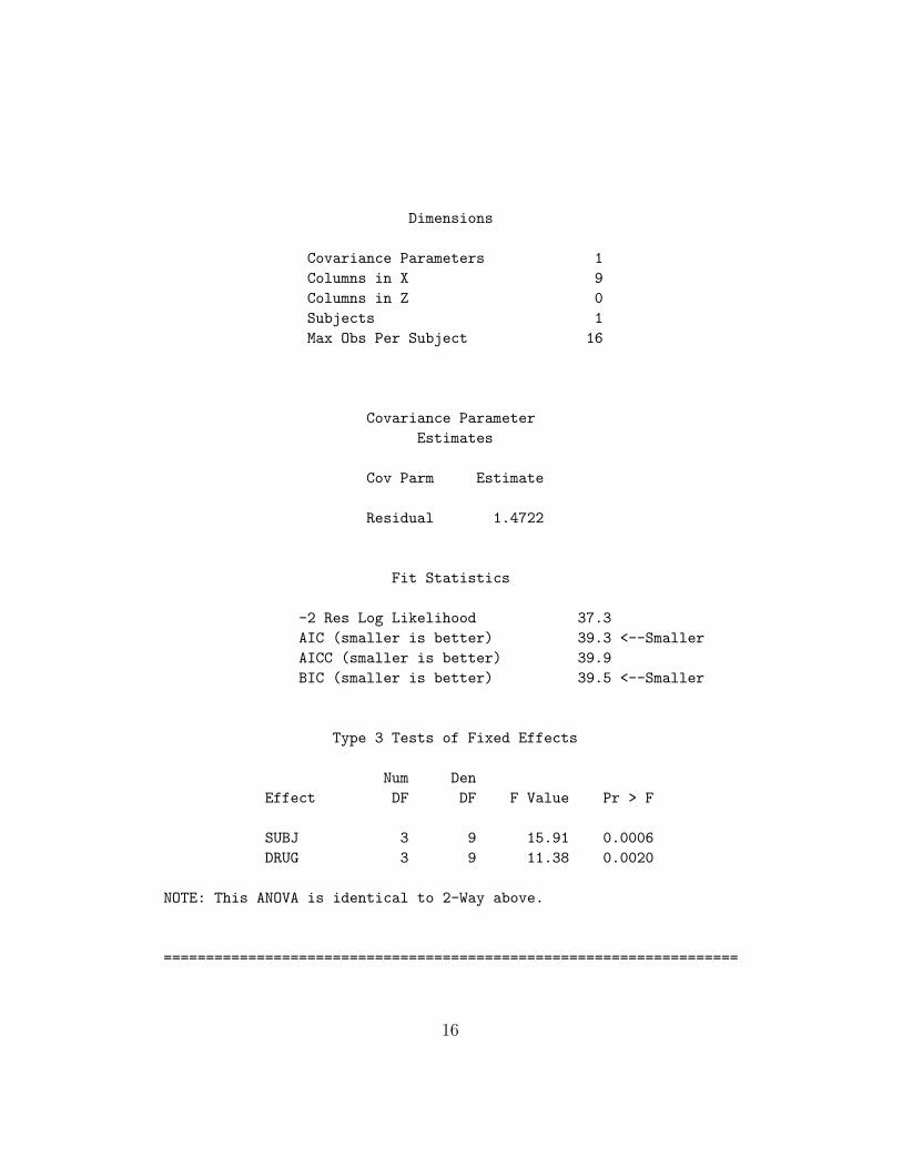
Dimensions
Covariance Parameters 1
Columns in X 9
Columns in Z 0
Subjects 1
Max Obs Per Subject 16
Covariance Parameter
Estimates
Cov Parm Estimate
Residual 1.4722
Fit Statistics
-2 Res Log Likelihood 37.3
AIC (smaller is better) 39.3 <--Smaller
AICC (smaller is better) 39.9
BIC (smaller is better) 39.5 <--Smaller
Type 3 Tests of Fixed Effects
Num Den
Effect DF DF F Value Pr > F
SUBJ 3 9 15.91 0.0006
DRUG 3 9 11.38 0.0020
NOTE: This ANOVA is identical to 2-Way above.
====================================================================
16
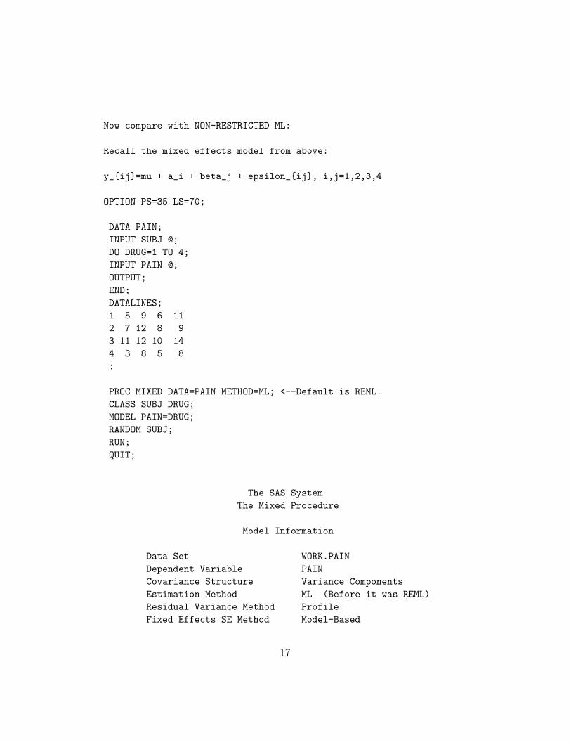
Now compare with NON-RESTRICTED ML:
Recall the mixed effects model from above:
y_{ij}=mu + a_i + beta_j + epsilon_{ij}, i,j=1,2,3,4
OPTION PS=35 LS=70;
DATA PAIN;
INPUT SUBJ @;
DO DRUG=1 TO 4;
INPUT PAIN @;
OUTPUT;
END;
DATALINES;
1 5 9 6 11
2 7 12 8 9
3 11 12 10 14
4 3 8 5 8
;
PROC MIXED DATA=PAIN METHOD=ML; <--Default is REML.
CLASS SUBJ DRUG;
MODEL PAIN=DRUG;
RANDOM SUBJ;
RUN;
QUIT;
The SAS System
The Mixed Procedure
Model Information
Data Set WORK.PAIN
Dependent Variable PAIN
Covariance Structure Variance Components
Estimation Method ML (Before it was REML)
Residual Variance Method Profile
Fixed Effects SE Method Model-Based
17
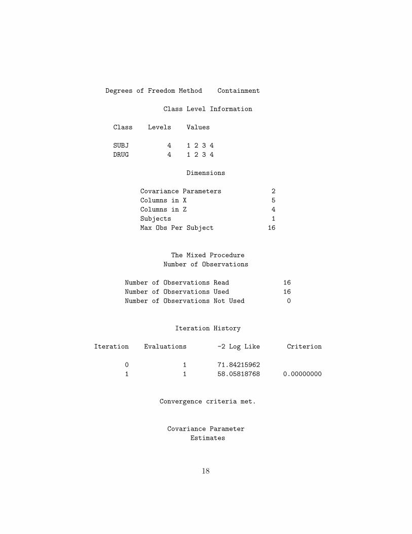
Degrees of Freedom Method Containment
Class Level Information
Class Levels Values
SUBJ 4 1 2 3 4
DRUG 4 1 2 3 4
Dimensions
Covariance Parameters 2
Columns in X 5
Columns in Z 4
Subjects 1
Max Obs Per Subject 16
The Mixed Procedure
Number of Observations
Number of Observations Read 16
Number of Observations Used 16
Number of Observations Not Used 0
Iteration History
Iteration Evaluations -2 Log Like Criterion
0 1 71.84215962
1 1 58.05818768 0.00000000
Convergence criteria met.
Covariance Parameter
Estimates
18

Cov Parm Estimate
SUBJ 4.1146 (With REML get 5.4861)
Residual 1.1042 (With REML get 1.4722)
Fit Statistics
-2 Log Likelihood 58.1 (With REML get 52.5)
AIC (smaller is better) 70.1 (With REML get 56.5)
AICC (smaller is better) 79.4
BIC (smaller is better) 66.4
Type 3 Tests of Fixed Effects
Num Den
Effect DF DF F Value Pr > F
DRUG 3 9 15.17 0.0007 (With REML get 0.002)
=====================================================================
Ex2. Two-Factor Repeated Experiment:
Repeated measure on one factor.
--------------------------------------
Subjects are randomly assigned to control or treatment group. Then
each subject is measured befored (PRE) and after (POST) treatment.
The treatment for the conrol group is a placebo or no treatment at
all.
GROUP SUBJ PRE POST
----------------------------
1 80 83
Control 2 85 86
3 83 88
---------------------------- NOTE: Subject nested within group!
4 82 94
Treatment 5 87 93
19
6 84 98
----------------------------
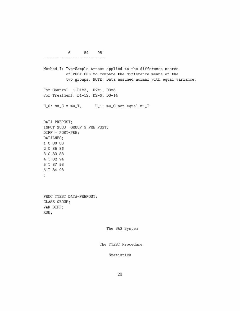
Method I: Two-Sample t-test applied to the difference scores
of POST-PRE to compare the difference means of the
two groups. NOTE: Data assumed normal with equal variance.
For Control : D1=3, D2=1, D3=5
For Treatment: D1=12, D2=6, D3=14
H_0: mu_C = mu_T, H_1: mu_C not equal mu_T
DATA PREPOST;
INPUT SUBJ GROUP $ PRE POST;
DIFF = POST-PRE;
DATALNES;
1 C 80 83
2 C 85 86
3 C 83 88
4 T 82 94
5 T 87 93
6 T 84 98
;
PROC TTEST DATA=PREPOST;
CLASS GROUP;
VAR DIFF;
RUN;
The SAS System
The TTEST Procedure
Statistics
20
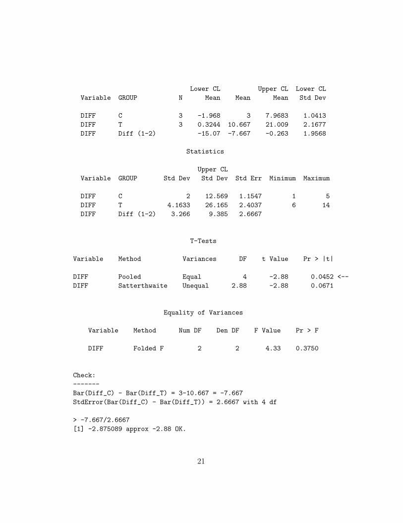
Lower CL Upper CL Lower CL
Variable GROUP N Mean Mean Mean Std Dev
DIFF C 3 -1.968 3 7.9683 1.0413
DIFF T 3 0.3244 10.667 21.009 2.1677
DIFF Diff (1-2) -15.07 -7.667 -0.263 1.9568
Statistics
Upper CL
Variable GROUP Std Dev Std Dev Std Err Minimum Maximum
DIFF C 2 12.569 1.1547 1 5
DIFF T 4.1633 26.165 2.4037 6 14
DIFF Diff (1-2) 3.266 9.385 2.6667
T-Tests
Variable Method Variances DF t Value Pr > |t|
DIFF Pooled Equal 4 -2.88 0.0452 <--
DIFF Satterthwaite Unequal 2.88 -2.88 0.0671
Equality of Variances
Variable Method Num DF Den DF F Value Pr > F
DIFF Folded F 2 2 4.33 0.3750
Check:
-------
Bar(Diff_C) - Bar(Diff_T) = 3-10.667 = -7.667
StdError(Bar(Diff_C) - Bar(Diff_T)) = 2.6667 with 4 df
> -7.667/2.6667
[1] -2.875089 approx -2.88 OK.
21
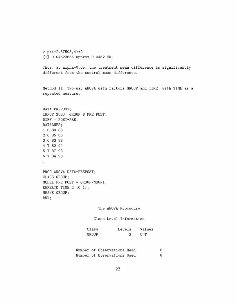
> pt(-2.87508,4)*2
[1] 0.04523655 approx 0.0452 OK.
Thus, at alpha=0.05, the treatment mean difference is significantly
different from the control mean difference.
Method II: Two-way ANOVA with factors GROUP and TIME, with TIME as a
repeated measure.
DATA PREPOST;
INPUT SUBJ GROUP $ PRE POST;
DIFF = POST-PRE;
DATALNES;
1 C 80 83
2 C 85 86
3 C 83 88
4 T 82 94
5 T 87 93
6 T 84 98
;
PROC ANOVA DATA=PREPOST;
CLASS GROUP;
MODEL PRE POST = GROUP/NOUNI;
REPEATD TIME 2 (0 1);
MEANS GROUP;
RUN;
The ANOVA Procedure
Class Level Information
Class Levels Values
GROUP 2 C T
Number of Observations Read 6
Number of Observations Used 6
22
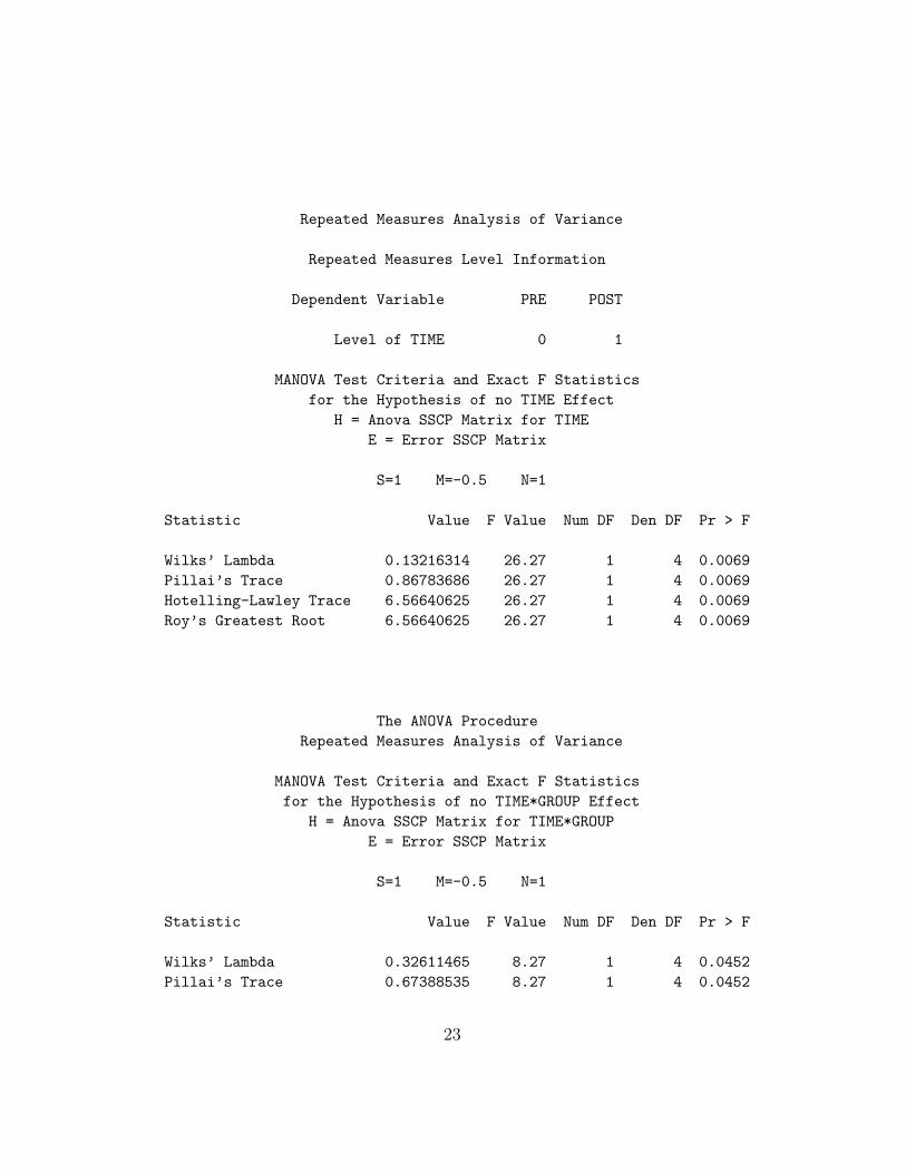
Repeated Measures Analysis of Variance
Repeated Measures Level Information
Dependent Variable PRE POST
Level of TIME 0 1
MANOVA Test Criteria and Exact F Statistics
for the Hypothesis of no TIME Effect
H = Anova SSCP Matrix for TIME
E = Error SSCP Matrix
S=1 M=-0.5 N=1
Statistic Value F Value Num DF Den DF Pr > F
Wilks’ Lambda 0.13216314 26.27 1 4 0.0069
Pillai’s Trace 0.86783686 26.27 1 4 0.0069
Hotelling-Lawley Trace 6.56640625 26.27 1 4 0.0069
Roy’s Greatest Root 6.56640625 26.27 1 4 0.0069
The ANOVA Procedure
Repeated Measures Analysis of Variance
MANOVA Test Criteria and Exact F Statistics
for the Hypothesis of no TIME*GROUP Effect
H = Anova SSCP Matrix for TIME*GROUP
E = Error SSCP Matrix
S=1 M=-0.5 N=1
Statistic Value F Value Num DF Den DF Pr > F
Wilks’ Lambda 0.32611465 8.27 1 4 0.0452
Pillai’s Trace 0.67388535 8.27 1 4 0.0452
23
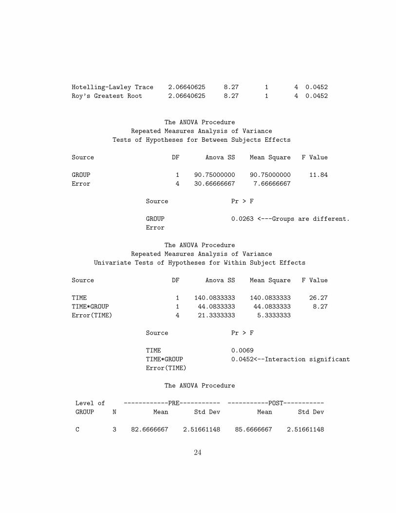
Hotelling-Lawley Trace 2.06640625 8.27 1 4 0.0452
Roy’s Greatest Root 2.06640625 8.27 1 4 0.0452
The ANOVA Procedure
Repeated Measures Analysis of Variance
Tests of Hypotheses for Between Subjects Effects
Source DF Anova SS Mean Square F Value
GROUP 1 90.75000000 90.75000000 11.84
Error 4 30.66666667 7.66666667
Source Pr > F
GROUP 0.0263 <---Groups are different.
Error
The ANOVA Procedure
Repeated Measures Analysis of Variance
Univariate Tests of Hypotheses for Within Subject Effects
Source DF Anova SS Mean Square F Value
TIME 1 140.0833333 140.0833333 26.27
TIME*GROUP 1 44.0833333 44.0833333 8.27
Error(TIME) 4 21.3333333 5.3333333
Source Pr > F
TIME 0.0069
TIME*GROUP 0.0452<--Interaction significant
Error(TIME)
The ANOVA Procedure
Level of ------------PRE----------- -----------POST-----------
GROUP N Mean Std Dev Mean Std Dev
C 3 82.6666667 2.51661148 85.6666667 2.51661148
24
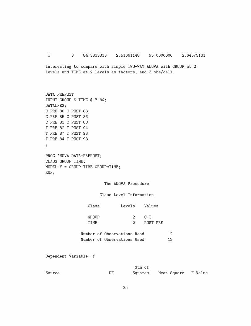
T 3 84.3333333 2.51661148 95.0000000 2.64575131
Interesting to compare with simple TWO-WAY ANOVA with GROUP at 2
levels and TIME at 2 levels as factors, and 3 obs/cell.
DATA PREPOST;
INPUT GROUP $ TIME $ Y @@;
DATALNES;
C PRE 80 C POST 83
C PRE 85 C POST 86
C PRE 83 C POST 88
T PRE 82 T POST 94
T PRE 87 T POST 93
T PRE 84 T POST 98
;
PROC ANOVA DATA=PREPOST;
CLASS GROUP TIME;
MODEL Y = GROUP TIME GROUP*TIME;
RUN;
The ANOVA Procedure
Class Level Information
Class Levels Values
GROUP 2 C T
TIME 2 POST PRE
Number of Observations Read 12
Number of Observations Used 12
Dependent Variable: Y
Sum of
Source DF Squares Mean Square F Value
25
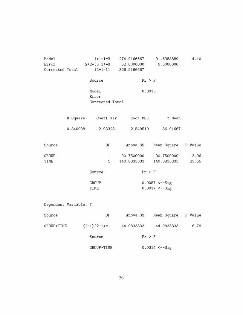
Model 1+1+1=3 274.9166667 91.6388889 14.10
Error 2*2*(3-1)=8 52.0000000 6.5000000
Corrected Total 12-1=11 326.9166667
Source Pr > F
Model 0.0015
Error
Corrected Total
R-Square Coeff Var Root MSE Y Mean
0.840938 2.933281 2.549510 86.91667
Source DF Anova SS Mean Square F Value
GROUP 1 90.7500000 90.7500000 13.96
TIME 1 140.0833333 140.0833333 21.55
Source Pr > F
GROUP 0.0057 <--Sig
TIME 0.0017 <--Sig
Dependent Variable: Y
Source DF Anova SS Mean Square F Value
GROUP*TIME (2-1)(2-1)=1 44.0833333 44.0833333 6.78
Source Pr > F
GROUP*TIME 0.0314 <--Sig
26