STAT 503 Case Study: Clustering of music clipsdicook/stat503/cs-music.pdf · STAT 503 Case Study: Clustering of music clips 1 ... tracks (8 rock, 3 classical, 1 new ... B1 All in

STAT 503 Case Study: Clustering of music clips

1 Description

This data was collected by Dr Cook from her own CDs. Using a Mac she read the track into the musicediting software Amadeus II, snipped and saved the first 40 seconds as a WAV file. (WAV is an audio formatdeveloped by Microsoft, commonly used on Windows but it is getting less popular.) These files were readinto R using the package tuneR. This converts the audio file into numeric data. All of the CDs contained leftand right channels, and variables were calculated on both channels. The resulting data has 62 rows (cases)and 7 columns (variables).

• LVar, LAve, LMax: average, variance, maximum of the frequencies of the left channel.

• LFEner: an indicator of the amplitude or loudness of the sound.

• LFreq: Median of the location of the 15 highest peak in the periodogram.

There are 11 tracks by Abba, 11 from the Beatles and 10 the Eels, which would be considered to beRock, and 13 tracks by Vivaldi, 6 of Mozart and 8 of Beethoven, considered to be Classical. There are also3 tracks from Enya, considered to be New Wave. The main question we want to answer is:

“Can we group the tracks into a small number of clusters according to their similarity on audio charac-tieristics?”

This information might be used to arrange tracks on a digital music player. Other questions of interest mightbe:

• Do the rock tracks have different characteristics than classical tracks?

• How does Enya compare to rock and classical tracks?

• Are there differences between the tracks of different artists?

1

2 Plan for Analysis

Approach Reason Type of questions addressedSummary statistics(marginal and condi-tional)

extract location/scale information “How are rock tracks different on av-erage than classical tracks?” “Whatis the average LAve for Abba relativeto other Artists?”

Plots explore data distributions “Are there unusual tracks?”, “Isthere any obvious clustering of thetracks?”

Numerical clustering Grouping the tracks into clusters ofsimilar audio attributes. Use hier-archical, k-means, model-based andself-organizing maps.

“Which tracks might be consideredalike?”

2

3 Results

3.1 Summary Statistics

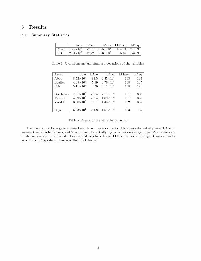
LVar LAve LMax LFEner LFreqMean 1.99×107 -7.81 2.25×104 104.03 231.39SD 2.64×107 47.22 8.76×103 5.48 176.69

Table 1: Overall means and standard deviations of the variables.

Artist LVar LAve LMax LFEner LFreqAbba 8.52×106 -81.5 2.35×104 103 135Beatles 4.45×107 -5.99 2.76×104 108 147Eels 5.11×107 4.59 3.13×104 108 181

Beethoven 7.61×106 -0.74 2.11×104 101 350Mozart 4.69×106 -5.94 1.89×104 101 396Vivaldi 3.00×106 39.1 1.45×104 102 305

Enya 5.03×107 -11.8 1.61×104 103 95

Table 2: Means of the variables by artist.

The classical tracks in general have lower LVar than rock tracks. Abba has substantially lower LAve onaverage than all other artists, and Vivaldi has substantially higher values on average. The LMax values aresimilar on average for all artists. Beatles and Eels have higher LFEner values on average. Classical trackshave lower LFreq values on average than rock tracks.

3

3.2 Plots

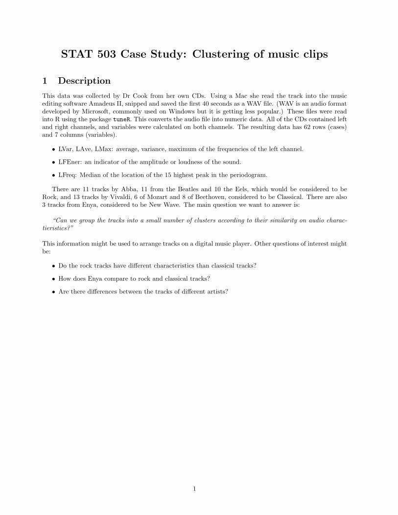
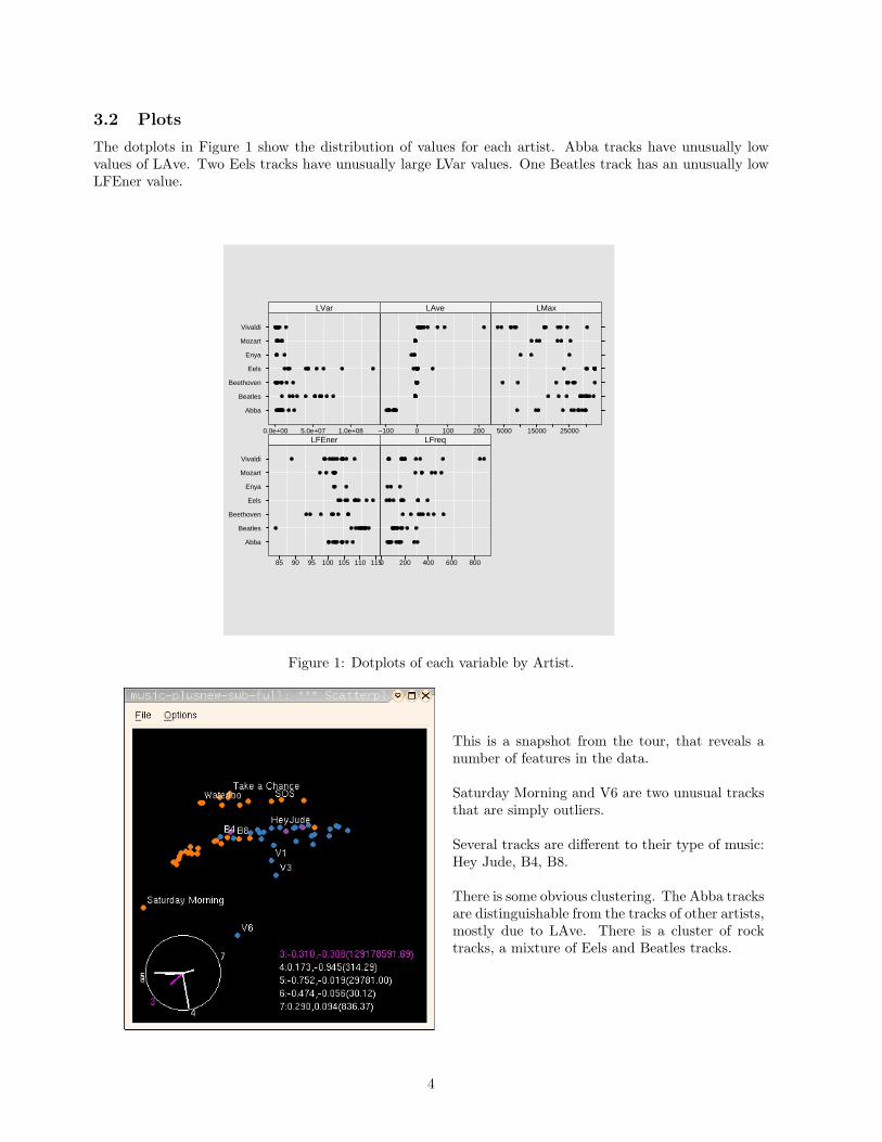
The dotplots in Figure 1 show the distribution of values for each artist. Abba tracks have unusually lowvalues of LAve. Two Eels tracks have unusually large LVar values. One Beatles track has an unusually lowLFEner value.

0.0e+00 5.0e+07 1.0e+08

Abba

Beatles

Beethoven

Eels

Enya

Mozart

Vivaldi

LVar

−100 0 100 200

LAve

5000 15000 25000

LMax

85 90 95 100 105 110 115

Abba

Beatles

Beethoven

Eels

Enya

Mozart

Vivaldi

LFEner

0 200 400 600 800

LFreq

Figure 1: Dotplots of each variable by Artist.

This is a snapshot from the tour, that reveals anumber of features in the data.

Saturday Morning and V6 are two unusual tracksthat are simply outliers.

Several tracks are different to their type of music:Hey Jude, B4, B8.

There is some obvious clustering. The Abba tracksare distinguishable from the tracks of other artists,mostly due to LAve. There is a cluster of rocktracks, a mixture of Eels and Beatles tracks.

4

4 Cluster Analysis

4.1 Hierarchical

Saturday MorningAll in a Days WorkYellow Submarine

Love of the LovelessWrong About Bobby

GirlCant Buy Me LoveRock Hard Times

I Feel FineHelp

Ticket to RidePenny Lane

Lone WolfI Want to Hold Your Hand

Love Me DoWaterloo

YesterdayB4

The Good Old DaysEleanor Rigby

Dancing QueenAgony

RestrainingAnywhere Is

V6B8B3

Mamma MiaM6B1

HeyJudeKnowing Me

Take a ChanceM3

V11Pax Deorum

M5B5

V10V8B2V4B6

The WinnerThe Memory of Trees

V5V2

V12V13M1M2V1V7B7

I Have A DreamSOS

Lay All YouMoney

V3Super Trouper

V9M4

0e+00 4e+08 8e+08

Ward

hclust (*, "ward")

Saturday MorningGirl

Knowing MeTake a Chance

M3B1

HeyJudeB3

Mamma MiaM6

V11Pax Deorum

M5B5


V5V2

V12V10V8B2V4B6

Lay All YouMoney

V3V13M1M2V1V7B7

I Have A DreamSOS

Super TrouperV9M4

RestrainingAnywhere Is

Dancing QueenThe Good Old Days

Eleanor RigbyAgony

V6B8

Love Me DoWaterloo

YesterdayB4

All in a Days WorkYellow Submarine


Cant Buy Me LoveTicket to Ride

Rock Hard TimesI Feel Fine

HelpPenny Lane


0e+00 2e+07 4e+07

Single

hclust (*, "single")m

usic.dist

Saturday MorningV13M1M2V1V7B7

I Have A DreamSOSV11

Pax DeorumM5B5

V10V8B2V4B6


V5V2

V12Knowing Me

Take a ChanceM3B1

HeyJudeB3

Mamma MiaM6

Lay All YouMoney

V9M4

Super TrouperV3

Love Me DoWaterloo

YesterdayB4

Dancing QueenThe Good Old Days

Eleanor RigbyRestraining

Anywhere IsAgony

V6B8

GirlCant Buy Me Love

Ticket to RideAll in a Days WorkYellow Submarine


Rock Hard TimesI Feel Fine

HelpPenny Lane


0.0e+00 6.0e+07 1.2e+08

Com

plete

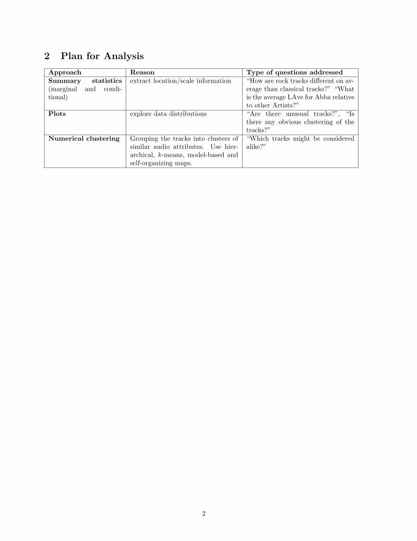
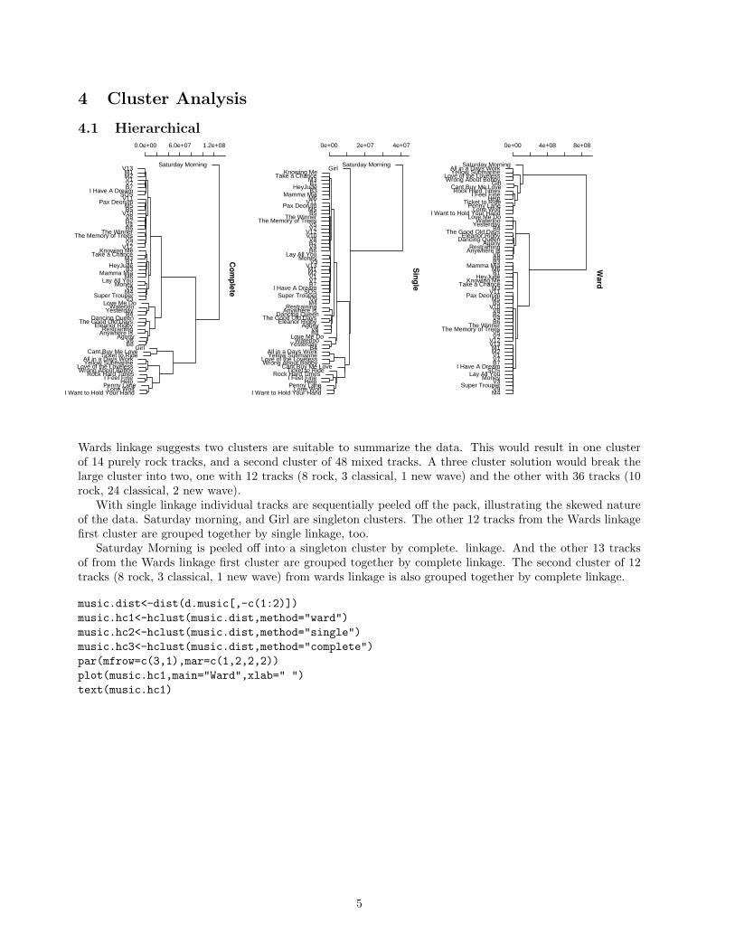
Wards linkage suggests two clusters are suitable to summarize the data. This would result in one clusterof 14 purely rock tracks, and a second cluster of 48 mixed tracks. A three cluster solution would break thelarge cluster into two, one with 12 tracks (8 rock, 3 classical, 1 new wave) and the other with 36 tracks (10rock, 24 classical, 2 new wave).

With single linkage individual tracks are sequentially peeled off the pack, illustrating the skewed natureof the data. Saturday morning, and Girl are singleton clusters. The other 12 tracks from the Wards linkagefirst cluster are grouped together by single linkage, too.

Saturday Morning is peeled off into a singleton cluster by complete. linkage. And the other 13 tracksof from the Wards linkage first cluster are grouped together by complete linkage. The second cluster of 12tracks (8 rock, 3 classical, 1 new wave) from wards linkage is also grouped together by complete linkage.

music.dist<-dist(d.music[,-c(1:2)])music.hc1<-hclust(music.dist,method="ward")music.hc2<-hclust(music.dist,method="single")music.hc3<-hclust(music.dist,method="complete")par(mfrow=c(3,1),mar=c(1,2,2,2))plot(music.hc1,main="Ward",xlab=" ")text(music.hc1)

5

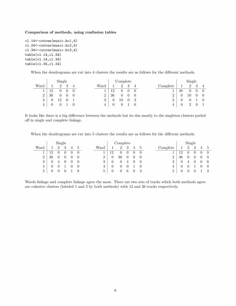
Comparison of methods, using confusion tables

cl.14<-cutree(music.hc1,4)cl.24<-cutree(music.hc2,4)cl.34<-cutree(music.hc3,4)table(cl.14,cl.24)table(cl.14,cl.34)table(cl.34,cl.24)

When the dendrograms are cut into 4 clusters the results are as follows for the different methods.

SingleWard 1 2 3 4

1 12 0 0 02 36 0 0 03 0 12 0 14 0 0 1 0

CompleteWard 1 2 3 4

1 12 0 0 02 36 0 0 03 0 10 0 34 0 0 1 0

SingleComplete 1 2 3 4

1 48 0 0 02 0 10 0 03 0 0 1 04 0 2 0 1

It looks like there is a big difference between the methods but its due mostly to the singleton clusters peeledoff in single and complete linkage.

When the dendrograms are cut into 5 clusters the results are as follows for the different methods.

SingleWard 1 2 3 4 5

1 12 0 0 0 02 36 0 0 0 03 0 4 0 0 04 0 0 1 0 05 0 0 0 1 8

CompleteWard 1 2 3 4 5

1 12 0 0 0 02 0 36 0 0 03 0 0 4 0 04 0 0 0 1 05 0 0 6 0 3

SingleComplete 1 2 3 4 5

1 12 0 0 0 02 36 0 0 0 03 0 4 0 0 64 0 0 1 0 05 0 0 0 1 2

Wards linkage and complete linkage agree the most. There are two sets of tracks which both methods agreeare cohesive clusters (labeled 1 and 2 by both methods) with 12 and 36 tracks respectively.

6

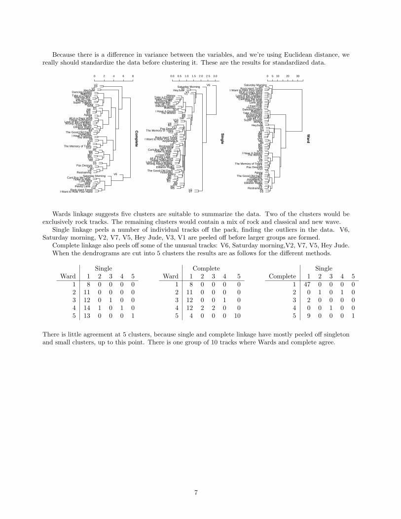
Because there is a difference in variance between the variables, and we’re using Euclidean distance, wereally should standardize the data before clustering it. These are the results for standardized data.

Saturday MorningGirl

Rock Hard TimesI Want to Hold Your Hand




Lone WolfHelp

I Feel FinePenny Lane

Dancing QueenWaterloo

Take a ChanceKnowing MeMamma MiaLay All You

Super TrouperMoney

V5HeyJude

V2V7B4

B1M6M3B3

V10M2B6

M1M5M4B5

SOSI Have A Dream

The WinnerV4B2V8

V11The Memory of Trees

V12Pax Deorum

V13V6

AgonyB8

The Good Old DaysYesterday

Anywhere IsLove Me Do

Eleanor RigbyB7V9

RestrainingV1V3

0 5 10 20 30

Ward

hclust (*, "ward")

V6Saturday Morning

V5HeyJude

V3V1

MoneyTake a ChanceSuper TrouperKnowing Me

Mamma MiaLay All YouDancing Queen

WaterlooSOS

I Have A DreamThe Winner

B6B4

GirlV10M2

V4B2

V13Pax Deorum

The Memory of TreesV12

V8V11


Anywhere IsB7

V9RestrainingLone Wolf


HelpI Feel Fine

Penny LaneAll in a Days WorkYellow Submarine


Love Me DoEleanor Rigby

B8The Good Old Days

YesterdayAgonyB1M6

M3B3

B5M4

M1M5

V2V7

0.0 0.5 1.0 1.5 2.0 2.5 3.0

Single

hclust (*, "single")m

usic.dist

V2V7

V5HeyJude

Dancing QueenWaterloo

Take a ChanceMamma MiaLay All YouKnowing Me

Super TrouperMoney

SOSB4

M6M3B3

AgonyB1



Love Me DoEleanor Rigby

Anywhere IsB8

The Good Old DaysYesterday

I Have A DreamThe Winner

V8V11V4B2

The Memory of TreesV12

B6M4B5

M1M5V10M2

V1V3

Pax DeorumV13

B7V9

RestrainingV6

Saturday MorningCant Buy Me Love

Ticket to RideLone Wolf

HelpI Feel Fine

Penny LaneGirl


0 2 4 6 8

Com

plete

Wards linkage suggests five clusters are suitable to summarize the data. Two of the clusters would beexclusively rock tracks. The remaining clusters would contain a mix of rock and classical and new wave.

Single linkage peels a number of individual tracks off the pack, finding the outliers in the data. V6,Saturday morning, V2, V7, V5, Hey Jude, V3, V1 are peeled off before larger groups are formed.

Complete linkage also peels off some of the unusual tracks: V6, Saturday morning,V2, V7, V5, Hey Jude.When the dendrograms are cut into 5 clusters the results are as follows for the different methods.

SingleWard 1 2 3 4 5

1 8 0 0 0 02 11 0 0 0 03 12 0 1 0 04 14 1 0 1 05 13 0 0 0 1

CompleteWard 1 2 3 4 5

1 8 0 0 0 02 11 0 0 0 03 12 0 0 1 04 12 2 2 0 05 4 0 0 0 10

SingleComplete 1 2 3 4 5

1 47 0 0 0 02 0 1 0 1 03 2 0 0 0 04 0 0 1 0 05 9 0 0 0 1

There is little agreement at 5 clusters, because single and complete linkage have mostly peeled off singletonand small clusters, up to this point. There is one group of 10 tracks where Wards and complete agree.

7

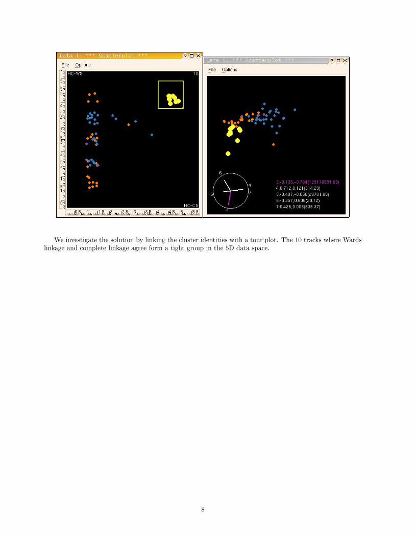
We investigate the solution by linking the cluster identities with a tour plot. The 10 tracks where Wardslinkage and complete linkage agree form a tight group in the 5D data space.

8

4.2 k-means

k-means clustering, with k = 2, . . . , 14 is computed on the data. The 5 cluster solution is given below.

k-meansWards 1 2 3 4 5

1 0 0 0 8 02 0 0 9 2 03 3 1 5 1 34 0 0 0 0 165 14 0 0 0 0

The results match for roughly 47out of 62 cases. The mappingfrom Wards to k-means is as fol-lows:1 → 4 (8 tracks)2 → 3 (9 tracks)4 → 5 (16 tracks)5 → 1 (14 tracks)Which allows us to rearrange theconfusion table.

k-meansWards 1 2 3 4 5

5 14 0 0 0 03 3 1 5 1 32 0 0 9 2 01 0 0 0 8 04 0 0 0 0 16

The 5-cluster results of k-means agree substantially with Wards linkage hierarchical clustering. Thesimilar groupings are:

Wards k-means Tracks5 1 All in a Days Work, Saturday Morning, Love of the Loveless, Girl,

Rock Hard Times, Lone Wolf, Wrong About Bobby, I Want to HoldYour Hand, Cant Buy Me Love, I Feel Fine, Ticket to Ride, Help,Yellow Submarine, Penny Lane

2 3 The Winner, V4, V8, B2, The Memory of Trees, Pax Deorum, V11,V12, V13

1 4 Dancing Queen, Knowing Me, Take a Chance, Mamma Mia, LayAll You, Super Trouper, Money, Waterloo

4 5 V2, V5, V7, V10, M1, M2, M3, M4, M5, M6, B1, B3, B4, B5, B6,HeyJude

The results are interesting: 8 of the 11 Abba tracks are in one cluster (W1,K4), one cluster containspurely rock tracks (W5,K1), and one cluster contains all classical tracks except for the unusual Beatles trackHey Jude (W4,K5).

library(mva)music.km2<-kmeans(d.music.std[,-c(1,2)],2)table(cl.15,music.km5$cluster)

9

4.3 SOM

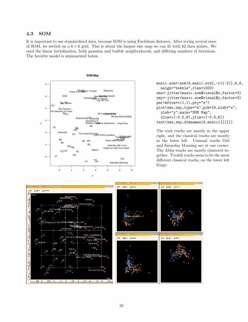
It is important to use standardized data, because SOM is using Euclidean distance. After trying several sizesof SOM, we settled on a 6 × 6 grid. This is about the largest size map we can fit with 62 data points. Weused the linear initialization, both gaussian and bubble neighborhoods, and differing numbers of iterations.The favorite model is summarized below.

0 1 2 3 4 5 6

01

23

45

6

SOM Map

x

y

Dancing QueenKnowing MeTake a Chance

Mamma Mia

Lay All You

Super TrouperI Have A Dream

The Winner

Money

SOS

V1

V2

V3

V4

V5

V6

V7

V8

V9

V10

M1

M2

M3

M4

M5

M6

All in a Days Work

Saturday Morning

The Good Old DaysLove of the Loveless

Girl

Agony

Rock Hard Times

Restraining

Lone Wolf

Wrong About BobbyLove Me Do

I Want to Hold Your HandCant Buy Me Love

I Feel Fine

Ticket to RideHelp

Yesterday

Yellow SubmarineEleanor Rigby

Penny Lane

B1

B2

B3

B4B5

B6

B7B8

The Memory of Trees

Anywhere Is

Pax Deorum

Waterloo

V11

V12

V13

HeyJude

music.som<-som(d.music.std[,-c(1:2)],6,6,neigh="bubble",rlen=1000)

xmx<-jitter(music.som$visual$x,factor=3)xmy<-jitter(music.som$visual$y,factor=3)par(mfrow=c(1,1),pty="s")plot(xmx,xmy,type="n",pch=16,xlab="x",ylab="y",main="SOM Map",xlim=c(-0.5,6),ylim=c(-0.5,6))

text(xmx,xmy,dimnames(d.music)[[1]])

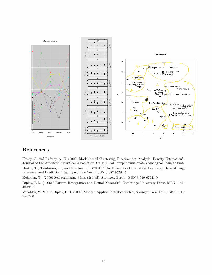
The rock tracks are mostly in the upperright, and the classical tracks are mostlyin the lower left. Unusual tracks Girland Saturday Morning are at one corner.The Abba tracks are mostly clustered to-gether. Vivaldi tracks seem to be the mostdifferent classical tracks, on the lower leftfringe.

10

4.4 Model-based

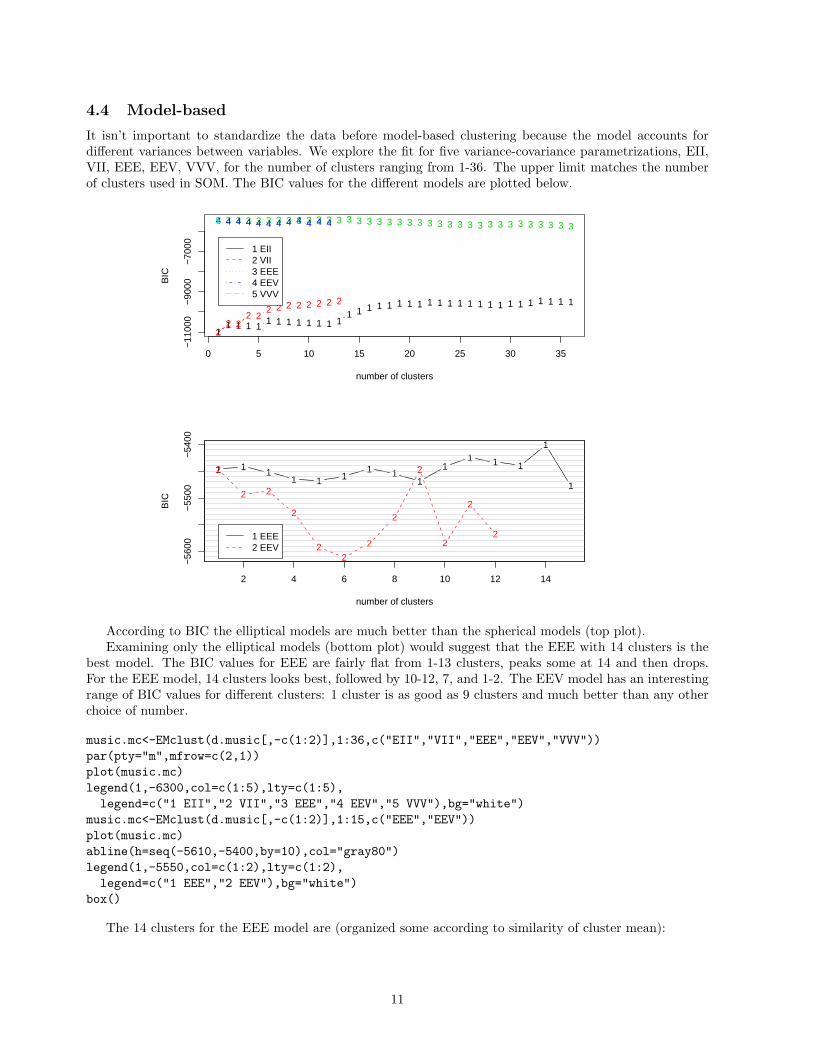
It isn’t important to standardize the data before model-based clustering because the model accounts fordifferent variances between variables. We explore the fit for five variance-covariance parametrizations, EII,VII, EEE, EEV, VVV, for the number of clusters ranging from 1-36. The upper limit matches the numberof clusters used in SOM. The BIC values for the different models are plotted below.

11 1 1 1

1 1 1 1 1 1 1 11 1 1 1 1 1 1 1 1 1 1 1 1 1 1 1 1 1 1 1 1 1 1

0 5 10 15 20 25 30 35

−11

000

−90

00−

7000

number of clusters

BIC

22 2

2 22 2 2 2 2 2 2 2

3 3 3 3 3 3 3 3 3 3 3 3 3 3 3 3 3 3 3 3 3 3 3 3 3 3 3 3 3 3 3 3 3 3 3 34 4 4 4 4 4 4 4 4 4 4 45

1 EII2 VII3 EEE4 EEV5 VVV

1 1 11 1 1

1 11

11 1 1

1

1

2 4 6 8 10 12 14

−56

00−

5500

−54

00

number of clusters

BIC

2

2 2

2

22

2

2

2

2

2

21 EEE2 EEV

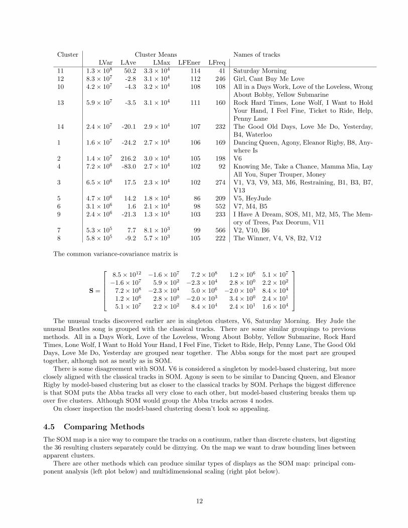
According to BIC the elliptical models are much better than the spherical models (top plot).Examining only the elliptical models (bottom plot) would suggest that the EEE with 14 clusters is the

best model. The BIC values for EEE are fairly flat from 1-13 clusters, peaks some at 14 and then drops.For the EEE model, 14 clusters looks best, followed by 10-12, 7, and 1-2. The EEV model has an interestingrange of BIC values for different clusters: 1 cluster is as good as 9 clusters and much better than any otherchoice of number.

music.mc<-EMclust(d.music[,-c(1:2)],1:36,c("EII","VII","EEE","EEV","VVV"))par(pty="m",mfrow=c(2,1))plot(music.mc)legend(1,-6300,col=c(1:5),lty=c(1:5),legend=c("1 EII","2 VII","3 EEE","4 EEV","5 VVV"),bg="white")

music.mc<-EMclust(d.music[,-c(1:2)],1:15,c("EEE","EEV"))plot(music.mc)abline(h=seq(-5610,-5400,by=10),col="gray80")legend(1,-5550,col=c(1:2),lty=c(1:2),legend=c("1 EEE","2 EEV"),bg="white")

box()

The 14 clusters for the EEE model are (organized some according to similarity of cluster mean):

11

Cluster Cluster Means Names of tracksLVar LAve LMax LFEner LFreq

11 1.3× 108 50.2 3.3× 104 114 41 Saturday Morning12 8.3× 107 -2.8 3.1× 104 112 246 Girl, Cant Buy Me Love10 4.2× 107 -4.3 3.2× 104 108 108 All in a Days Work, Love of the Loveless, Wrong

About Bobby, Yellow Submarine13 5.9× 107 -3.5 3.1× 104 111 160 Rock Hard Times, Lone Wolf, I Want to Hold

Your Hand, I Feel Fine, Ticket to Ride, Help,Penny Lane

14 2.4× 107 -20.1 2.9× 104 107 232 The Good Old Days, Love Me Do, Yesterday,B4, Waterloo

1 1.6× 107 -24.2 2.7× 104 106 169 Dancing Queen, Agony, Eleanor Rigby, B8, Any-where Is

2 1.4× 107 216.2 3.0× 104 105 198 V64 7.2× 106 -83.0 2.7× 104 102 92 Knowing Me, Take a Chance, Mamma Mia, Lay

All You, Super Trouper, Money3 6.5× 106 17.5 2.3× 104 102 274 V1, V3, V9, M3, M6, Restraining, B1, B3, B7,

V135 4.7× 106 14.2 1.8× 104 86 209 V5, HeyJude6 3.1× 106 1.6 2.1× 104 98 552 V7, M4, B59 2.4× 106 -21.3 1.3× 104 103 233 I Have A Dream, SOS, M1, M2, M5, The Mem-

ory of Trees, Pax Deorum, V117 5.3× 105 7.7 8.1× 103 99 566 V2, V10, B68 5.8× 105 -9.2 5.7× 103 105 222 The Winner, V4, V8, B2, V12

The common variance-covariance matrix is

S =

8.5× 1012 −1.6× 107 7.2× 108 1.2× 106 5.1× 107

−1.6× 107 5.9× 102 −2.3× 104 2.8× 100 2.2× 102

7.2× 108 −2.3× 104 5.0× 106 −2.0× 103 8.4× 104

1.2× 106 2.8× 100 −2.0× 103 3.4× 100 2.4× 101

5.1× 107 2.2× 102 8.4× 104 2.4× 101 1.6× 104

The unusual tracks discovered earlier are in singleton clusters, V6, Saturday Morning. Hey Jude the

unusual Beatles song is grouped with the classical tracks. There are some similar groupings to previousmethods. All in a Days Work, Love of the Loveless, Wrong About Bobby, Yellow Submarine, Rock HardTimes, Lone Wolf, I Want to Hold Your Hand, I Feel Fine, Ticket to Ride, Help, Penny Lane, The Good OldDays, Love Me Do, Yesterday are grouped near together. The Abba songs for the most part are groupedtogether, although not as neatly as in SOM.

There is some disagreement with SOM. V6 is considered a singleton by model-based clustering, but moreclosely aligned with the classical tracks in SOM. Agony is seen to be similar to Dancing Queen, and EleanorRigby by model-based clustering but as closer to the classical tracks by SOM. Perhaps the biggest differenceis that SOM puts the Abba tracks all very close to each other, but model-based clustering breaks them upover five clusters. Although SOM would group the Abba tracks across 4 nodes.

On closer inspection the model-based clustering doesn’t look so appealing.

4.5 Comparing Methods

The SOM map is a nice way to compare the tracks on a contiuum, rather than discrete clusters, but digestingthe 36 resulting clusters separately could be dizzying. On the map we want to draw bounding lines betweenapparent clusters.

There are other methods which can produce similar types of displays as the SOM map: principal com-ponent analysis (left plot below) and multidimensional scaling (right plot below).

12

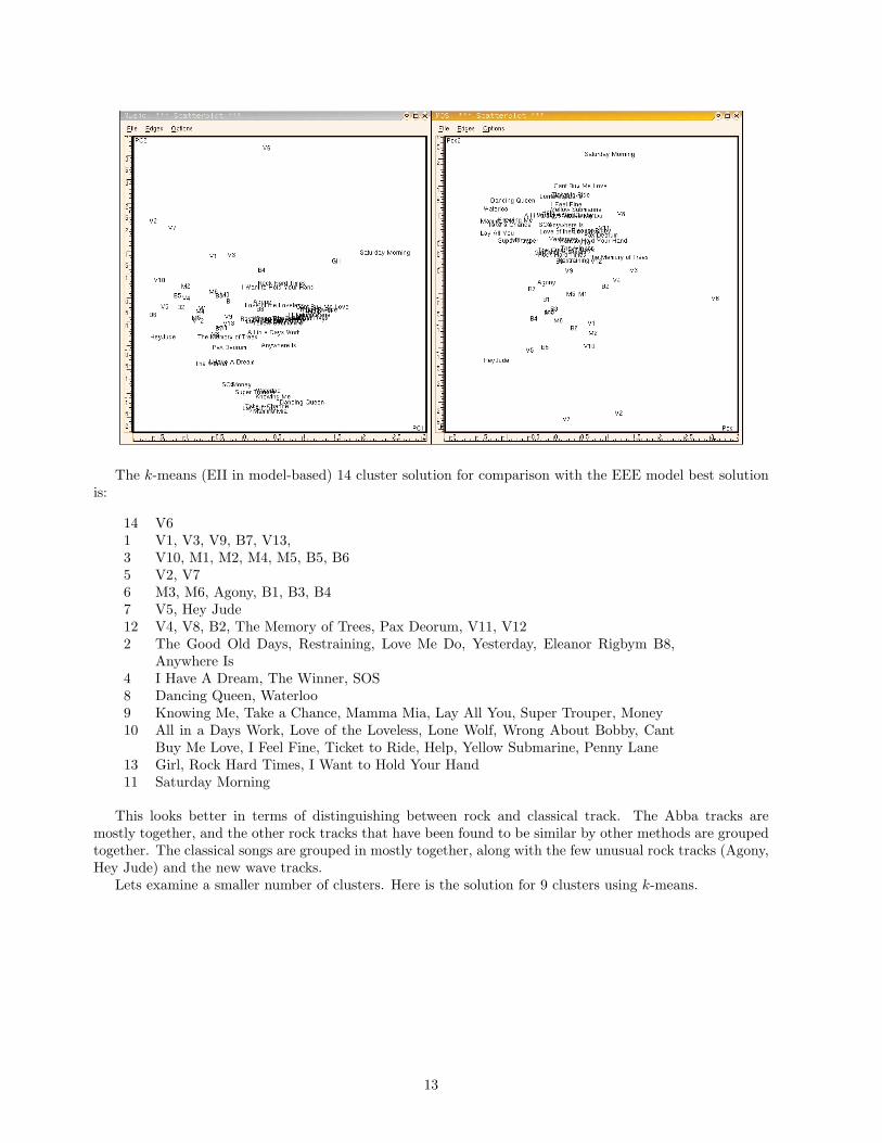
The k-means (EII in model-based) 14 cluster solution for comparison with the EEE model best solutionis:

14 V61 V1, V3, V9, B7, V13,3 V10, M1, M2, M4, M5, B5, B65 V2, V76 M3, M6, Agony, B1, B3, B47 V5, Hey Jude12 V4, V8, B2, The Memory of Trees, Pax Deorum, V11, V122 The Good Old Days, Restraining, Love Me Do, Yesterday, Eleanor Rigbym B8,

Anywhere Is4 I Have A Dream, The Winner, SOS8 Dancing Queen, Waterloo9 Knowing Me, Take a Chance, Mamma Mia, Lay All You, Super Trouper, Money10 All in a Days Work, Love of the Loveless, Lone Wolf, Wrong About Bobby, Cant

Buy Me Love, I Feel Fine, Ticket to Ride, Help, Yellow Submarine, Penny Lane13 Girl, Rock Hard Times, I Want to Hold Your Hand11 Saturday Morning

This looks better in terms of distinguishing between rock and classical track. The Abba tracks aremostly together, and the other rock tracks that have been found to be similar by other methods are groupedtogether. The classical songs are grouped in mostly together, along with the few unusual rock tracks (Agony,Hey Jude) and the new wave tracks.

Lets examine a smaller number of clusters. Here is the solution for 9 clusters using k-means.

13

6 V69 V2, V75 V10, M1, M2, M4, M5, B5, B67 V1, V9, M3, M6, Agony, Restraining, B1, B3, B4, B72 V5, HeyJude3 The Winner, V3, V4, V8, B2, The Memory of Trees, Pax Deorum, V11, V12, V131 Dancing Queen, Knowing Me, Take a Chance, Mamma Mia, Lay All You, Super

Trouper, I Have A Dream, Money, SOS, Waterloo4 All in a Days Work, The Good Old Days, Love of the Loveless, Wrong About Bobby,

Love Me Do, Yesterday, Yellow Submarine, Eleanor Rigby, B8, Anywhere Is8 Saturday Morning, Girl, Rock Hard Times, Lone Wolf, I Want to Hold Your Hand,

Cant Buy Me Love, I Feel Fine, Ticket to Ride, Help, Penny Lane

BUT Saturday Morning is not in its own cluster. Here is the solution for 10 clusters:

10 V62 V2, V7, V10, M25 V1, M3, M6, Agony, B1, B3, B41 V5, M4, M5, B5, B6, B7, HeyJude4 V3, V4, V8, M1, B2, The Memory of Trees, Pax Deorum, V11, V12, V138 I Have A Dream, The Winner, SOS3 Dancing Queen, Knowing Me, Take a Chance, Mamma Mia, Lay All You, Super

Trouper, Money, Waterloo6 V9, The Good Old Days, Restraining, Love Me Do, Yesterday, Eleanor Rigby, B8,

Anywhere Is7 All in a Days Work, Love of the Loveless, Girl, Rock Hard Times, Lone Wolf, Wrong

About Bobby, I Want to Hold Your Hand, Cant Buy Me Love, I Feel Fine, Ticketto Ride, Help, Yellow Submarine, Penny Lane

9 Saturday Morning

14

5 Conclusions

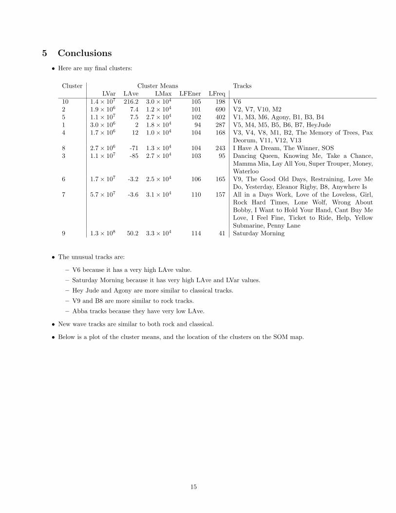
• Here are my final clusters:

Cluster Cluster Means TracksLVar LAve LMax LFEner LFreq

10 1.4× 107 216.2 3.0× 104 105 198 V62 1.9× 106 7.4 1.2× 104 101 690 V2, V7, V10, M25 1.1× 107 7.5 2.7× 104 102 402 V1, M3, M6, Agony, B1, B3, B41 3.0× 106 2 1.8× 104 94 287 V5, M4, M5, B5, B6, B7, HeyJude4 1.7× 106 12 1.0× 104 104 168 V3, V4, V8, M1, B2, The Memory of Trees, Pax

Deorum, V11, V12, V138 2.7× 106 -71 1.3× 104 104 243 I Have A Dream, The Winner, SOS3 1.1× 107 -85 2.7× 104 103 95 Dancing Queen, Knowing Me, Take a Chance,

Mamma Mia, Lay All You, Super Trouper, Money,Waterloo

6 1.7× 107 -3.2 2.5× 104 106 165 V9, The Good Old Days, Restraining, Love MeDo, Yesterday, Eleanor Rigby, B8, Anywhere Is

7 5.7× 107 -3.6 3.1× 104 110 157 All in a Days Work, Love of the Loveless, Girl,Rock Hard Times, Lone Wolf, Wrong AboutBobby, I Want to Hold Your Hand, Cant Buy MeLove, I Feel Fine, Ticket to Ride, Help, YellowSubmarine, Penny Lane

9 1.3× 108 50.2 3.3× 104 114 41 Saturday Morning

• The unusual tracks are:

– V6 because it has a very high LAve value.

– Saturday Morning because it has very high LAve and LVar values.

– Hey Jude and Agony are more similar to classical tracks.

– V9 and B8 are more similar to rock tracks.

– Abba tracks because they have very low LAve.

• New wave tracks are similar to both rock and classical.

• Below is a plot of the cluster means, and the location of the clusters on the SOM map.

15

Variables

LVar LAve LMax LFEner LFreq

12345678910

Cluster means

−4−2

024

LVarLAveLMaxLFEnerLFreq

1−4−2024

2−4−2

024

3−4−2024

4−4−2

024

5−4−2024

6−4−2

024

7−4−2024

8−4−2

024

9−4−2024

10

References

Fraley, C. and Raftery, A. E. (2002) Model-based Clustering, Discriminant Analysis, Density Estimation”,Journal of the American Statistical Association, 97, 611–631, http://www.stat.washington.edu/mclust.Hastie, T., Tibshirani, R., and Friedman, J. (2001) ”The Elements of Statistical Learning: Data Mining,Inference, and Prediction”, Springer, New York, ISBN 0 387 95284 5.Kohonen, T., (2000) Self-organizing Maps (3rd ed), Springer, Berlin, ISBN 3 540 67921 9.Ripley, B.D. (1996) ”Pattern Recognition and Neural Networks” Cambridge University Press, ISBN 0 52146086 7.Venables, W.N. and Ripley, B.D. (2002) Modern Applied Statistics with S, Springer, New York, ISBN 0 38795457 0.

16

Appendix

d.music<-read.csv("music-plusnew-sub-full.csv",row.names=1)apply(d.music[,-c(1,2)],2,mean)apply(d.music[,-c(1,2)],2,sd)d.music.std<-cbind(d.music[,c(1,2)],apply(d.music[,-c(1,2)],2,f.std.data))

# Summary statisticsapply(d.music[,-c(1,2)],2,mean)apply(d.music[,-c(1,2)],2,sd)

apply(d.music[d.music[,1]=="Abba",-c(1,2)],2,mean)apply(d.music[d.music[,1]=="Beatles",-c(1,2)],2,mean)apply(d.music[d.music[,1]=="Eels",-c(1,2)],2,mean)

apply(d.music[d.music[,1]=="Beethoven",-c(1,2)],2,mean)apply(d.music[d.music[,1]=="Mozart",-c(1,2)],2,mean)apply(d.music[d.music[,1]=="Vivaldi",-c(1,2)],2,mean)

apply(d.music[d.music[,1]=="Enya",-c(1,2)],2,mean)

# Plotslibrary(lattice)d.music.df<-data.frame(Artist=factor(rep(d.music[,1],5)),y=as.vector(as.matrix(d.music[,3:7])),meas=factor(rep(1:5, rep(62,5)), labels=names(d.music[,-c(1,2)])))

postscript("music-dotplot.ps",width=8.0,height=8.0,horizontal=FALSE,paper="special",family="URWHelvetica")

par(pty="s",mar=c(2,1,1,1))plt.bg<-trellis.par.get("background")plt.bg$col<-"grey90"trellis.par.set("background",plt.bg)stripplot(Artist~y|meas, data=d.music.df, scales=list(x="free"),strip=function(...) strip.default(style=1,...),panel=function(x,y){panel.grid(h=-1,v=5,col="white")panel.stripplot(x,y,col=1,pch=16)},

xlab="",pch=16,col=1,layout=c(3,2),aspect=1,as.table=T)

dev.off()

# Hierarchical clusteringmusic.dist<-dist(d.music[,-c(1:2)])music.dist<-dist(d.music.std[,-c(1:2)])music.hc1<-hclust(music.dist,method="ward")music.hc2<-hclust(music.dist,method="single")music.hc3<-hclust(music.dist,method="complete")postscript("music-hclust.ps",width=5.0,height=10.0,horizontal=FALSE,paper="special",family="URWHelvetica")

par(mfrow=c(3,1),mar=c(1,2,2,2))plot(music.hc1,main="Ward",xlab=" ")text(music.hc1)plot(music.hc2,main="Single",ylab=" ")text(music.hc2)plot(music.hc3,main="Complete",ylab=" ")

17

text(music.hc3)dev.off()

cl.12<-cutree(music.hc1,2)cl.22<-cutree(music.hc2,2)cl.32<-cutree(music.hc3,2)













18

table(cl.12,cl.22)table(cl.12,cl.32)table(cl.32,cl.22)table(cl.13,cl.23)table(cl.13,cl.33)table(cl.33,cl.23)table(cl.14,cl.24)table(cl.14,cl.34)table(cl.34,cl.24)table(cl.15,cl.25)table(cl.15,cl.35)table(cl.35,cl.25)table(cl.16,cl.26)table(cl.16,cl.36)table(cl.36,cl.26)table(cl.17,cl.27)table(cl.17,cl.37)table(cl.37,cl.27)table(cl.18,cl.28)table(cl.18,cl.38)table(cl.38,cl.28)table(cl.19,cl.29)table(cl.19,cl.39)table(cl.39,cl.29)table(cl.110,cl.210)table(cl.110,cl.310)table(cl.310,cl.210)table(cl.111,cl.211)table(cl.111,cl.311)table(cl.311,cl.211)table(cl.112,cl.212)table(cl.112,cl.312)table(cl.312,cl.212)table(cl.113,cl.213)table(cl.113,cl.313)table(cl.313,cl.213)table(cl.114,cl.214)table(cl.114,cl.314)table(cl.314,cl.214)

for (i in 1:5)cat(i,",",dimnames(d.music)[[1]][cl.15==i],"\n")

for (i in 1:5)cat(i,",",dimnames(d.music)[[1]][music.km5$cluster==i],"\n")

dimnames(d.music)[[1]][music.km5$cluster==3&cl.15==2]

library(genegobitree)library(Rggobi)ggobi()setup.gobidend(music.hc1,d.music)color.click.dn(music.hc1,d.music)

19

library(mva)music.km2<-kmeans(d.music.std[,-c(1,2)],2)music.km3<-kmeans(d.music.std[,-c(1,2)],3)music.km4<-kmeans(d.music.std[,-c(1,2)],4)music.km5<-kmeans(d.music.std[,-c(1,2)],5)music.km6<-kmeans(d.music.std[,-c(1,2)],6)music.km7<-kmeans(d.music.std[,-c(1,2)],7)music.km8<-kmeans(d.music.std[,-c(1,2)],8)music.km9<-kmeans(d.music.std[,-c(1,2)],9)music.km10<-kmeans(d.music.std[,-c(1,2)],10)music.km11<-kmeans(d.music.std[,-c(1,2)],11)music.km12<-kmeans(d.music.std[,-c(1,2)],12)music.km13<-kmeans(d.music.std[,-c(1,2)],13)music.km14<-kmeans(d.music.std[,-c(1,2)],14)

table(cl.15,music.km5$cluster)

d.music.clust1<-cbind(d.music,cl.12,cl.22,cl.32,cl.13,cl.23,cl.33,cl.14,cl.24,cl.34,cl.15,cl.25,cl.35,cl.16,cl.26,cl.36,cl.17,cl.27,cl.37,cl.18,cl.28,cl.38,music.km2$cluster,music.km3$cluster,music.km4$cluster,music.km5$cluster,music.km6$cluster,music.km7$cluster,music.km8$cluster)

dimnames(d.music.clust1)[[2]][8]<-"HC-W2"dimnames(d.music.clust1)[[2]][9]<-"HC-S2"dimnames(d.music.clust1)[[2]][10]<-"HC-C2"dimnames(d.music.clust1)[[2]][11]<-"HC-W3"dimnames(d.music.clust1)[[2]][12]<-"HC-S3"dimnames(d.music.clust1)[[2]][13]<-"HC-C3"dimnames(d.music.clust1)[[2]][14]<-"HC-W4"dimnames(d.music.clust1)[[2]][15]<-"HC-S4"dimnames(d.music.clust1)[[2]][16]<-"HC-C4"dimnames(d.music.clust1)[[2]][17]<-"HC-W5"dimnames(d.music.clust1)[[2]][18]<-"HC-S5"dimnames(d.music.clust1)[[2]][19]<-"HC-C5"dimnames(d.music.clust1)[[2]][20]<-"HC-W6"dimnames(d.music.clust1)[[2]][21]<-"HC-S6"dimnames(d.music.clust1)[[2]][22]<-"HC-C6"dimnames(d.music.clust1)[[2]][23]<-"HC-W7"dimnames(d.music.clust1)[[2]][24]<-"HC-S7"dimnames(d.music.clust1)[[2]][25]<-"HC-C7"dimnames(d.music.clust1)[[2]][26]<-"HC-W8"dimnames(d.music.clust1)[[2]][27]<-"HC-S8"dimnames(d.music.clust1)[[2]][28]<-"HC-C8"dimnames(d.music.clust1)[[2]][29]<-"KM-2"dimnames(d.music.clust1)[[2]][30]<-"KM-3"dimnames(d.music.clust1)[[2]][31]<-"KM-4"dimnames(d.music.clust1)[[2]][32]<-"KM-5"dimnames(d.music.clust1)[[2]][33]<-"KM-6"dimnames(d.music.clust1)[[2]][34]<-"KM-7"dimnames(d.music.clust1)[[2]][35]<-"KM-8"f.writeXML(d.music.clust1,"music-clust1.xml",data.num=1)

for (i in 1:6)

20

cat(i,",",dimnames(d.music)[[1]][music.km6$cluster==i],"\n")

music.som<-som(d.music.std[,-c(1:2)],6,6,rlen=100)music.som<-som(d.music.std[,-c(1:2)],6,6,rlen=200)music.som<-som(d.music.std[,-c(1:2)],6,6,rlen=300)music.som<-som(d.music.std[,-c(1:2)],6,6,rlen=400)music.som<-som(d.music.std[,-c(1:2)],6,6,rlen=1000)music.som<-som(d.music.std[,-c(1:2)],6,6,neigh="bubble",rlen=100)music.som<-som(d.music.std[,-c(1:2)],6,6,neigh="bubble",rlen=200)music.som<-som(d.music.std[,-c(1:2)],6,6,neigh="bubble",rlen=300)music.som<-som(d.music.std[,-c(1:2)],6,6,neigh="bubble",rlen=400)music.som<-som(d.music.std[,-c(1:2)],6,6,neigh="bubble",rlen=1000)music.som<-som(d.music.std[,-c(1:2)],6,6,init="random",neigh="bubble",rlen=100)music.som<-som(d.music.std[,-c(1:2)],6,6,init="random",neigh="bubble",rlen=1000)

xmx<-jitter(music.som$visual$x,factor=3)xmy<-jitter(music.som$visual$y,factor=3)par(mfrow=c(1,1),pty="s")plot(xmx,xmy,type="n",pch=16,xlab="x",ylab="y",main="SOM Map",xlim=c(-0.5,6),ylim=c(-0.5,6))

text(xmx,xmy,dimnames(d.music)[[1]])dimnames(music.som$code)<-list(NULL,names(d.music[,-c(1,2)]))d.music.clust<-cbind(d.music.std,xmx,xmy)dimnames(d.music.clust)[[2]][8]<-"Map 1"dimnames(d.music.clust)[[2]][9]<-"Map 2"d.music.grid<-cbind(rep("0",36),rep("0",36),music.som$code,music.som$code.sum[,1:2])

dimnames(d.music.grid)[[2]][1]<-"Artist"dimnames(d.music.grid)[[2]][2]<-"Type"dimnames(d.music.grid)[[2]][8]<-"Map 1"dimnames(d.music.grid)[[2]][9]<-"Map 2"d.music.clust<-rbind(d.music.grid,d.music.clust)f.writeXML(d.music.clust,"music-SOM.xml",data.num=2,dat1.id<-c(1:dim(d.music.clust)[1]),dat2=cbind(c(1:60),c(1:60)),dat2.source=x33.l[,1],dat2.destination=x33.l[,2],dat2.name="SOM",dat2.id=paste(rep("l",60),c(1:60)))

# Favorite modelmusic.som<-som(d.music[,-c(1:2)],6,6,neigh="bubble",rlen=1000)music.som<-som(d.music.std[,-c(1:2)],6,6,neigh="bubble",rlen=1000)xmx<-jitter(music.som$visual$x,factor=3)xmy<-jitter(music.som$visual$y,factor=3)postscript("music-som.ps",width=8.0,height=8.0,horizontal=FALSE,paper="special",family="URWHelvetica")

par(mfrow=c(1,1),pty="s")plot(xmx,xmy,type="n",pch=16,xlab="x",ylab="y",main="SOM Map",xlim=c(-0.5,6),ylim=c(-0.5,6))

text(xmx,xmy,dimnames(d.music)[[1]])dev.off()

# Setting up the net lines

21

n.nodes<-6x33.l<-NULLfor (i in 1:n.nodes) {for (j in 1:n.nodes) {if (j<n.nodes) x33.l<-rbind(x33.l,c((i-1)*n.nodes+j,(i-1)*n.nodes+j+1))if (i<n.nodes) x33.l<-rbind(x33.l,c((i-1)*n.nodes+j,i*n.nodes+j))

}}

# Model-basedpostscript("music-mc1.ps",width=8.0,height=8.0,horizontal=FALSE,paper="special",family="URWHelvetica")

music.mc<-EMclust(d.music[,-c(1:2)],1:36,c("EII","VII","EEE","EEV","VVV"))par(pty="m",mfrow=c(2,1))plot(music.mc)legend(1,-6300,col=c(1:5),lty=c(1:5),legend=c("1 EII","2 VII","3 EEE","4 EEV","5 VVV"),bg="white")

music.mc<-EMclust(d.music[,-c(1:2)],1:15,c("EEE","EEV"))plot(music.mc)abline(h=seq(-5610,-5400,by=10),col="gray80")legend(1,-5550,col=c(1:2),lty=c(1:2),legend=c("1 EEE","2 EEV"),bg="white")

box()dev.off()smry<-summary(music.mc,d.music[,-c(1:2)])cl<-smry$classificationcl.mat<-matrix(0,62,2)cl.mat[cl==1,1]<-1cl.mat[cl==2,2]<-1prm<-mstepEEV(d.music[,-c(1:2)],cl.mat)d.music[cl==1,1:2]d.music[cl==2,1:2]

for (i in 1:14)cat(i,",",dimnames(d.music)[[1]][cl==i],"\n")

smry<-summary(music.mc,d.music[,-c(1:2)])smryt(smry$mu)smry$sigma

mc.clust.dist<-dist(t(smry$mu))mc.clust.mean<-hclust(mc.clust.dist,method="single")plot(mc.clust.mean)

music.mc<-EMclust(d.music[,-c(1:2)],11,"EEV")

music.mc2<-EMclust(d.music[,-c(1:2)],2,"EEE")summary(music.mc2,d.music[,-c(1:2)])music.mc3<-EMclust(d.music[,-c(1:2)],7,"EEE")summary(music.mc3,d.music[,-c(1:2)])mccl<-summary(music.mc3,d.music[,-c(1:2)])$classificationfor (i in 1:7)cat(i,",",dimnames(d.music)[[1]][mccl==i],"\n")

22

# Generate the ellipses in 5Dvc<-smry$sigma[,,1]evc<-eigen(vc)vc2<-(evc$vectors)%*%diag(sqrt(evc$values))%*%t(evc$vectors)y1<-f.gen.sphere(500,5)y1<-y1%*%vc2y1[,1]<-y1[,1]+smry$mu[1,1]y1[,2]<-y1[,2]+smry$mu[2,1]y1[,3]<-y1[,3]+smry$mu[3,1]y1[,4]<-y1[,4]+smry$mu[4,1]y1[,5]<-y1[,5]+smry$mu[5,1]vc<-smry$sigma[,,2]evc<-eigen(vc)vc2<-(evc$vectors)%*%diag(sqrt(evc$values))%*%t(evc$vectors)y2<-f.gen.sphere(500,5)y2<-y2%*%vc2y2[,1]<-y2[,1]+smry$mu[1,2]y2[,2]<-y2[,2]+smry$mu[2,2]y2[,3]<-y2[,3]+smry$mu[3,2]y2[,4]<-y2[,4]+smry$mu[4,2]y2[,5]<-y2[,5]+smry$mu[5,2]

y<-cbind(rep(0,1000),c(rep(1,500),rep(2,500)),rbind(y1,y2))

y[,1]<-factor(y[,1])y[,2]<-factor(y[,2])dimnames(y)<-list(NULL,names(d.music))

d.music.mc<-rbind(d.music,y)

f.writeXML(d.music.mc,"music-mclust.xml",data.num=1)

# Set up a full data setkmcl6<-music.km6$clusterdimnames(music.som$code)<-list(NULL,names(d.music[,-c(1,2)]))d.music.clust<-cbind(d.music,cl6,kmcl6,xmx,xmy)dimnames(d.music.clust)[[2]][8]<-"HC-W6"dimnames(d.music.clust)[[2]][9]<-"KM-6"dimnames(d.music.clust)[[2]][10]<-"Map 1"dimnames(d.music.clust)[[2]][11]<-"Map 2"d.music.grid<-cbind(rep("0",36),rep("0",36),music.som$code,rep(0,36),rep(0,36),music.som$code.sum[,1:2])

dimnames(d.music.grid)[[2]][1]<-"Artist"dimnames(d.music.grid)[[2]][2]<-"Type"dimnames(d.music.grid)[[2]][8]<-"HC-W6"dimnames(d.music.grid)[[2]][9]<-"KM-6"dimnames(d.music.grid)[[2]][10]<-"Map 1"dimnames(d.music.grid)[[2]][11]<-"Map 2"d.music.clust<-rbind(d.music.grid,d.music.clust)f.writeXML(d.music.clust,"SOM-music.xml",data.num=2,dat1.id<-c(1:dim(d.music.clust)[1]),dat2=cbind(c(1:60),c(1:60)),dat2.source=x33.l[,1],

23

dat2.destination=x33.l[,2],dat2.name="SOM",dat2.id=paste(rep("l",60),c(1:60)))

# Utility functionsf.gen.sphere<-function(n=100,p=5) {x<-matrix(rnorm(n*p),ncol=p)xnew<-t(apply(x,1,norm.vec))xnew}

norm.vec<-function(x) {x<-x/norm(x)x}

norm<-function(x) { sqrt(sum(x^2))}

# Out put data for ggvisedges<-NULLk<-1for (i in 1:61)for (j in (i+1):62) {edges<-rbind(edges,c(i,j,music.dist[k]))k<-k+1

}f.writeXML(d.music.std,"music-MDS.xml",data.num=2,dat1.id<-c(1:62),dat1.name="Music",dat2=cbind(1:1891,edges[,3]),dat2.source=edges[,1],dat2.destination=edges[,2],dat2.name="dist",dat2.id=c(1:1891))

# Comparison of clustersfor (i in 1:14)cat(i,",",dimnames(d.music)[[1]][music.km14$cluster==i],"\n")

# Check smaller number of clustersfor (i in 1:9)cat(i,",",dimnames(d.music)[[1]][music.km9$cluster==i],"\n")



options(digits=2)for (i in 1:10)cat(i,",",apply(d.music[music.km10$cluster==i,-c(1,2)],2,mean),"\n")

km10.mn<-NULLfor (i in 1:10)km10.mn<-rbind(km10.mn,apply(d.music[music.km10$cluster==i,-c(1,2)],2,mean))

24

km10.mn.std<-apply(km10.mn,2,f.std.data)range(km10.mn.std)postscript("music-means.ps",width=5.0,height=8.0,horizontal=FALSE,paper="special",family="URWHelvetica")

plot(c(1,5),c(-2.5,2.8),type="n",axes=F,xlab="Variables",ylab="")rect(0.8,-2.8,5.2,3.1,col="gray80")abline(v=c(1:5),col="white")abline(h=seq(-2.5,2.5,by=0.5),col="white")clrs<-c(1:7,9:11)for (i in 1:10) {lines(c(1:5),km10.mn.std[i,],lty=i,col=clrs[i])points(c(1:5),km10.mn.std[i,],pch=i,col=clrs[i])

}axis(side=1,at=c(1:5),labels=names(d.music[,-c(1,2)]))legend(1,-0.8,lty=c(1:10),pch=c(1:10),col=clrs,legend=c(1:10),bg="gray80")

title("Cluster means")box()dev.off()

library(lattice)d.music.df<-data.frame(cluster=factor(rep(music.km10$cluster,5)),y=as.vector(as.matrix(d.music.std[,3:7])),meas=factor(rep(1:5, rep(62,5)), labels=names(d.music[,-c(1,2)])))

postscript("music-means2.ps",width=3.0,height=10.0,horizontal=FALSE,paper="special",family="URWHelvetica")

plt.bg<-trellis.par.get("background")plt.bg$col<-"grey90"trellis.par.set("background",plt.bg)xyplot(y~meas|cluster,data=d.music.df,xlab="",ylab="",box.ratio=1,layout=c(1,10),col=1,pch=16,panel=function(x,y){panel.grid(h=-1,v=5,col="white")panel.stripplot(x,y,col=1,pch=16)})

dev.off()

25

Documents

STAT 503 Case Study: Clustering of music clipsdicook/stat503/cs-music.pdf · STAT 503 Case Study: Clustering of music clips 1 ... tracks (8 rock, 3 classical, 1 new ... B1 All in