Embed Size (px)
Citation preview

Stat 562 course presentation 1
Analysis of ordinal repeated categorical response data by using
marginal model (Maximum likelihood approach)
by Abdul Salam
Instructor: K.C. CarriereStat 562

Stat 562 course presentation 2
Contents:• Introduction• Background of data• Objective of the study• Basic theory
– Marginal model– Model fitting using ML
• SAS Codes• Results• Conclusion

Stat 562 course presentation 3
Introduction• Definition
– Categorical data
– Repeated categorical data
– Advantages and Disadvantages of repeated Measurements Designs

Stat 562 course presentation 4
Definition• Categorical data
– Categorical data fits into a small number of discrete categories
(as opposed to continuous). Categorical data is either non-
ordered (nominal) such as gender or city, or ordered (ordinal)
such as high, medium, or low temperatures.

Stat 562 course presentation 5
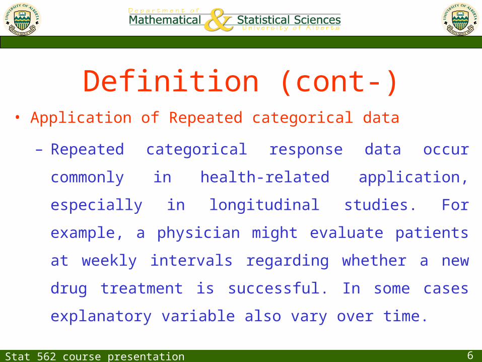
Definition (cont-)• Repeated categorical data
– The term “repeated measurements” refers broadly to data in
which the response of each experimental unit or subject is
observed on multiple occasions or under multiple conditions.
When the response is categorical then it is called repeated
categorical data.
Stat 562 course presentation 6
Definition (cont-)• Application of Repeated categorical data
– Repeated categorical response data occur commonly in health-
related application, especially in longitudinal studies. For
example, a physician might evaluate patients at weekly intervals
regarding whether a new drug treatment is successful. In some
cases explanatory variable also vary over time.

Stat 562 course presentation 7
Advantages of Repeated Measurements Designs • Individual patterns of change.
• Provide more efficient estimates of relevant parameters than cross-
sectional designs with the same number and pattern of
measurement.
• Between subjects sources of variability can be excluded from the
experimental error.

Stat 562 course presentation 8
Disadvantages of Repeated Measurements Designs
• Analysis of repeated data is complicated by the dependence among
the repeated observations made on the same experimental unit.
• Often investigator cannot control the circumstances for obtaining
measurements, so that the data may be unbalanced or partially
incomplete.
Stat 562 course presentation 9
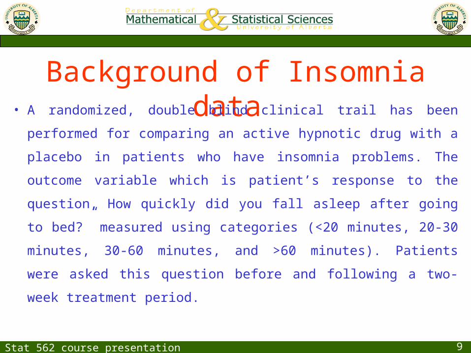
Background of Insomnia data • A randomized, double blind clinical trail has been performed for
comparing an active hypnotic drug with a placebo in patients
who have insomnia problems. The outcome variable which is
patient’s response to the question, How quickly did you fall
asleep after going to bed?” measured using categories (<20
minutes, 20-30 minutes, 30-60 minutes, and >60 minutes).
Patients were asked this question before and following a two-
week treatment period.

Stat 562 course presentation 10
Background of Insomnia data • Patients were randomly assigned to one of the two
treatments active and placebo. The two treatments, active
and placebo, form a binary explanatory variable. Patients
receiving the two treatments were independent samples.
Stat 562 course presentation 11
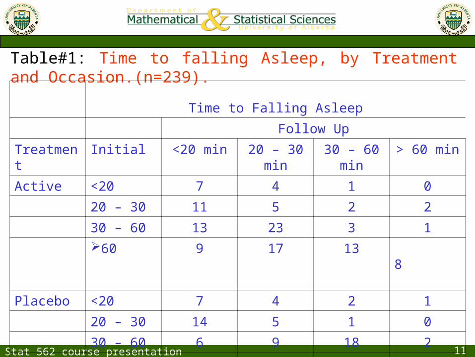
Table#1: Time to falling Asleep, by Treatment and Occasion.(n=239).
Time to Falling Asleep
Follow Up
Treatment Initial <20 min 20 – 30 min 30 – 60 min > 60 min
Active <20 7 4 1 0
20 – 30 11 5 2 2
30 – 60 13 23 3 1
60 9 17 13 8
Placebo <20 7 4 2 1
20 – 30 14 5 1 0
30 – 60 6 9 18 2
> 60 4 11 14 22

Stat 562 course presentation 12
Objectives
• To study the effect of time on the response.
• To study the effect of treatment on the response. Is the
time to fall asleep is quicker for active treatment than
placebo?
• Is there any interaction between treatment and time?
How does the treatment affect the time to fall asleep over
time?

Stat 562 course presentation 13
Pharmaceutical Company Interest
Company hope that patients with a Active treatment have
a significantly higher rate of improvement than patients
with placebo.

Stat 562 course presentation 14
Generalized linear model to the analysis of Repeated
Measurements Designs
• Marginal Models;
• Random Effect Models;
• Transition models.

Stat 562 course presentation 15
Basic Theory
Stat 562 course presentation 16
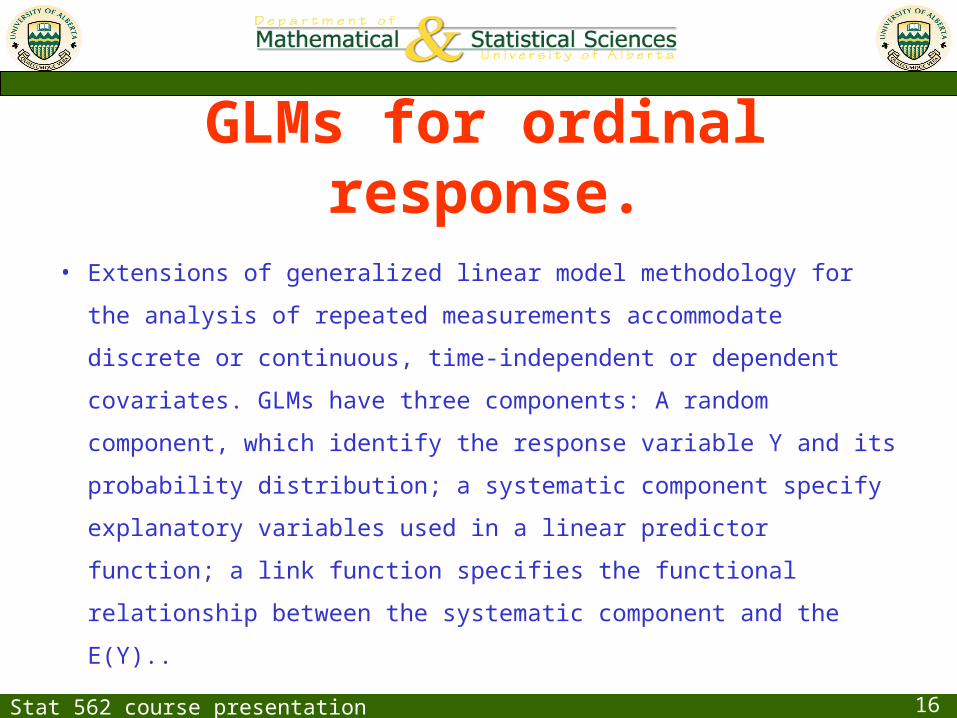
GLMs for ordinal response.
• Extensions of generalized linear model methodology for the
analysis of repeated measurements accommodate discrete or
continuous, time-independent or dependent covariates. GLMs
have three components: A random component, which identify
the response variable Y and its probability distribution; a
systematic component specify explanatory variables used in a
linear predictor function; a link function specifies the functional
relationship between the systematic component and the E(Y)..

Stat 562 course presentation 17
Random Component.• Since the response is ordinal, so it is often advantageous to
construct logits that account for categorical ordering and are less
affected by the number of choice of categories of the response,
which is known as cumulative response probabilities, from which the
cumulative logits are defined. For ordinal response with c + 1
ordered categories labeled as 0,1, 2,…….,C for each individuals or
experimental unit. The cumulative response probabilities are
( ),j rP Y j j = 0,1,…….c
Thus 0 1 1, ......., 1o o c

Stat 562 course presentation 18
Systematic component.
• The systematic component of the generalized linear model specifies
the explanatory variables. The linear combination of these
explanatory variables is called the linear predictor denoted by
0 1 1 2 2 ........i i i p ipx x x
The vector β characterizes how the cross-sectional response
distribution depends on the explanatory variables.

Stat 562 course presentation 19
Link Function.
• The link function explain the relation ship between
random and systematic component, that how
relates to the explanatory variables in the linear predictor.
For ordinal response having c+1 categories, one might use
the cumulative logit.
Logitj = logit [P(Y ≤ j)], j=1,…………..c
( )E y

Stat 562 course presentation 20
Link Function.1
1
log , 1,.......1
jj
j
j c
where j rP Y j
GLM is simplified to proportional odds model, then βj may
simplify to β indicating the same effect for each logit. The
proportional odds model is
j jx x for j =1,……….c,

Stat 562 course presentation 21
Link Function.For individuals with covariate vector x* and x, the odds ratio for the response below category j is
*
**
*
*
* *
* *
* *
* *
/
/,
/
/
exp,
exp
, exp
, exp
, exp
, exp .
r
rj
r
r
j
j
j
j j j
j j j
j
j
P Y j x
P Y j xx x
P Y j x
P Y j x
xx x
x
x x x x
x x x x
x x x x
x x x x
The odds ratio does not depend on response category j. The regression coefficient can be calculated by taking log, which indicate the difference in logit (log odds) of response variable per unit change in the x.

Stat 562 course presentation 22
Maximum Likelihood Method (ML).• The standard approach to maximum likelihood (ML) fitting of
marginal models involves solving the score equations using the
Newton-Raphson method, Fisher scoring, or some other iterative
reweighted least squares algorithm. ML fitting of marginal logit
models is awkward. For T observations on an I-category response,
at each setting of predictors the likelihood refers to IT multinomial
joint probabilities, but the model applies to T sets of marginal
multinomial parameters, and assume that marginal multinomial
variates are independent.

Stat 562 course presentation 23
ML: Model Speciofication.• Let consider T categorical responses, where the tth variable has
It categories. The responses are ordinal observed for P covariate
patterns, defined by a set of explanatory variables. Let r =
denote the number of response profiles for each covariate
pattern. The vector of counts for covariate pattern p is
denoted by Yp. The Yp are assumed to be independent
multinomial random vectors,
T
tt
I
, ;1 1 , 1,......,Tp p p r pY mult n p P

Stat 562 course presentation 24
ML: Model Speciofication.
• Where is a vector of positive probabilities and 1rT is a r-
dimensional vector of 1’s. Since the model applies to T sets of
marginal multinomial parameters, the marginal models can be
written as a generalized linear model with the link function,
logC A X
p

Stat 562 course presentation 25
ML Fitting of marginal Models: Lang and Agresti (1994) considered the likelihood as a function of
rather then. The likelihood function for a marginal logit model is the
product of the multinomial mass functions from the various predictors
setting. One approach for ML fitting views the model as a set of
constraints and uses methods for maximizing a function subject to
constraints log( ) 0U C A

Stat 562 course presentation 26
ML Fitting of marginal Models:
Let be a vector having elements and the lagrange multipliers . The Lagrangian likelihood equations have form
0h
, , logh h f l f
where
is a vector with terms involving the contents in marginal logits
that the model specifies constraints as well as log-likelihood
derivative. The Newton-Raphson iterative scheme is

Stat 562 course presentation 27
ML Fitting of marginal Models:
1
1 , 1,...............
t
t t th
h t
After obtaining the fitted values on convergence of the algorithm, they calculate model parameter estimates using
^ ^1
logX X X C A
This maximum likelihood fitting method makes no assumption about the model that describes the joint distribution. Thus, when the marginal model holds, the ML estimate are consistent regardless of the dependence structure for that distribution.

Stat 562 course presentation 28
InferenceHypothesis testing for parameters:• After obtaining model parameter estimates and estimated covariance
matrix, one can apply standard methods of inference, for instance Wald chi-squared test for marginal homogeneity.
Goodness of Fit test:• To assess model goodness of fit, one can compare observed and fitted
cell counts using the likelihood-ratio statistics G2 or the Pearson Chi-square statistics. For nonsparse tables, assuming that the model holds, these statistics have approximate chi-squared distributions with degree of freedom equal to the number of constraints implied by
logC A X

Stat 562 course presentation 29
Limitations of ML:• The number of multinomial probabilities increases
dramatically as the number of predictors increases.
• ML approaches are not practical when T is large or there are many predictors, especially when some are continuous.
• It does not make any assumption about the model that describes the joint distribution .
Stat 562 course presentation 30
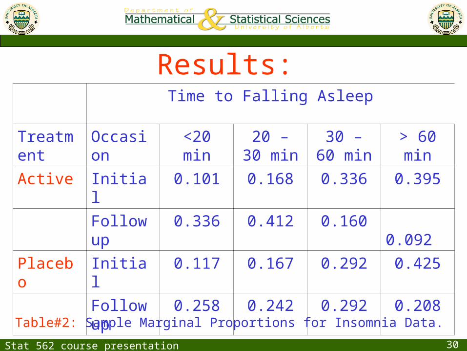
Results:
Table#2: Sample Marginal Proportions for Insomnia Data.
Time to Falling Asleep
Treatment Occasion <20 min 20 – 30 min
30 – 60 min
> 60 min
Active Initial 0.101 0.168 0.336 0.395
Follow up 0.336 0.412 0.160 0.092
Placebo Initial 0.117 0.167 0.292 0.425
Follow up 0.258 0.242 0.292 0.208
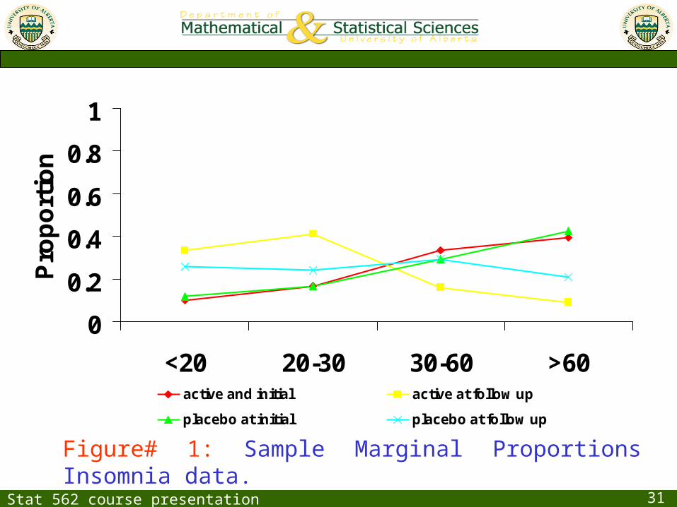
Stat 562 course presentation 31
Figure# 1: Sample Marginal Proportions Insomnia data.
0
0.2
0.4
0.6
0.8
1
<20 20-30 30-60 >60
Pro
po
rtio
n
active and initial active at follow up
placebo at initial placebo at follow up

Stat 562 course presentation 32
Marginal Proportion • sample proportion of time to falling asleep in <20 minutes for
subject who received Active treatment at initial occasion is
= (7+4+1+0) / (7+4+1+0+11+…………+13+8) = 12/119=0.1008
• Similarly the sample proportion of time to falling asleep in >60
minutes for subject received placebo at follow up is
= (1+0+2+22) / (7+4+2+1+………..+14+22) = 25/120=0.20833
And so on.

Stat 562 course presentation 33
What did you get from Marginal Proportion table?
• From initial to follow up occasion, time to falling asleep
seems to shift downward for both treatments.
• The degree of shift seems greater for the active treatment
than placebo, indicating possible interaction. Or we could
say that effect of treatment on the response is different at
different occasion.

Stat 562 course presentation 34
Fitted Marginal ModelLet ‘x’ represent the treatment, with x=1 for an Active treatment and x=0 for
the placebo. Let t denote the occasion measurement , with t=0 for initial and
t=1 for follow up. Let (Yt) represent the outcome variable which is patient’s
response at time t to the question, “How quickly did you fall asleep after
going to bed?” with j=0 for <20 minutes, j=1 for 20-30 minutes, j=2 for 30-60
minutes, and j=3 for >60 minutes). The marginal model with cumulative link
can be written for our data set as
1 2 3 *j t x x t logit [P(Y ≤ j)] =
Stat 562 course presentation 35
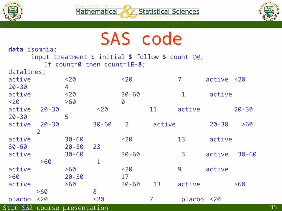
SAS codedata isomnia; input treatment $ initial $ follow $ count @@;
If count=0 then count=1E-8;datalines;active <20 <20 7 active <20 20-30 4active <20 30-60 1 active <20 >60 0 active 20-30 <20 11 active 20-30 20-30 5active 20-30 30-60 2 active 20-30 >60 2active 30-60 <20 13 active 30-60 20-30 23active 30-60 30-60 3 active 30-60 >60 1 active >60 <20 9 active >60 20-30 17active >60 30-60 13 active >60 >60 8placbo <20 <20 7 placbo <20 20-30 4placbo <20 30-60 2 placbo <20 >60 1 placbo 20-30 <20 14 placbo 20-30 20-30 5placbo 20-30 30-60 1 placbo 20-30 >60 0placbo 30-60 <20 6 placbo 30-60 20-30 9placbo 30-60 30-60 18 placbo 30-60 >60 2 placbo >60 <20 4 placbo >60 20-30 11placbo >60 30-60 14 placbo >60 >60 22;
Stat 562 course presentation 36
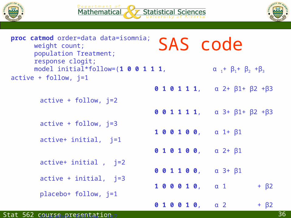
SAS codeproc catmod order=data data=isomnia; weight count; population Treatment; response clogit; model initial*follow=(1 0 0 1 1 1, α 1+ β1+ β2 +β3 active + follow, j=1
0 1 0 1 1 1, α 2+ β1+ β2 +β3 active + follow, j=2 0 0 1 1 1 1, α 3+ β1+ β2 +β3 active + follow, j=3 1 0 0 1 0 0, α 1+ β1 active+ initial, j=1
0 1 0 1 0 0, α 2+ β1 active+ initial , j=2 0 0 1 1 0 0, α 3+ β1 active + initial, j=3 1 0 0 0 1 0, α 1 + β2 placebo+ follow, j=1
0 1 0 0 1 0, α 2 + β2 placebo+ follow, j=2 0 0 1 0 1 0, α 3 + β2 placebo+ follow, j=3
1 0 0 0 0 0, α 1 placebo+ initial, j=1
0 1 0 0 0 0, α 2 placebo+ initial, j=2
0 0 1 0 0 0) α 3 placebo+ initial, j=3
(1 2 3 ='Cutpoint', 4='Treatment', 5='TIme effect', 6='Time*Treatment effect') / freq; quit;

Stat 562 course presentation 37
Fitted Marginal Model
After fitting the marginal model using maximum likelihood
method to the above marginal distribution gave the following
results
Logit [P (Y≤ J)] = -1.16+ 0.10 +1.37+1.074 (Occasion) +
0.046 (Treatment) +
0.662 (Occasion * Treatment)

Stat 562 course presentation 38
Hypothesis testing for estimators:• For Occasion
– β1= 1.074 S.E (β1)= 0.162 p-value=<0.0001
• For Treatment – β2= 0.046 S.E (β2)= 0.236 p-value= 0.84
• For interaction (Occasion * time) – β3= 0.662 S.E (β3)= 0.244 p-value= 0.00665

Stat 562 course presentation 39
Model Goodness of fit testThe Likelihood ratio test (G2) has been used for Goodness of fit
test. ML model fitting, comparing the observed to fitted cell
counts in modeling the 12 marginal logits using these six
parameters with df=6 gives G2 = 8.0 and p-value 0.238,
indicating that the model fit the given data set well

Stat 562 course presentation 40
Interpretation of ParametersEffect of Treatment: (Active vs Placebo)
• 1. At initial observation:
– The estimated odds that the time to falling asleep for the active
treatment is below any fixed equal Exp {0.046}=1.04 times the
estimated odds for the placebo treatment.
• 2. At Follow up observation:
– The estimated odds that the time to falling asleep for the active
treatment is below any fixed equal Exp{0.046+0.662} = 2.03 times
the estimated odds for the placebo treatment.

Stat 562 course presentation 41
Interpretation of Parameters (cont.)
• For the Active treatment the slope is β3= 0.662 (SE=0.244)
higher than for the placebo, giving strong evidence of faster
improvement. In other words, initially the two treatments had
similar effect, but at the follow up those patients with the active
treatment tended to fall asleep more quickly.

Stat 562 course presentation 42
Conclusion
Using the maximum likelihood methods for the marginal
distribution for the above given Insomnia data set, we have
sufficient evidence to conclude that treatment and time have
substantial effects on the response (time to fall asleep).

Stat 562 course presentation 43
Thank You For Your Attention