Stat

Examples: Random Variables and Probability Distributions

ENGSTAT Notes of AM Fillone

RANDOM VARIABLES and PROBABILITY DISTRIBUTIONS Example: Give the sample space giving a detailed description of each possible outcome when three electronic components are tested, where

N - denotes “nondefective” D - denotes “defective” Therefore, S = { NNN, NND, NDN, DNN, NDD, DND, DDN, DDD} The number of defectives that occur will be assigned a numerical value of 0, 1, 2, or 3, in the sample space. These values are random quantities determined by the outcome of the experiment. The random variable X - the no. of defective items when three electronic components are tested would be

Sample Space S NNN 0 NND 1 NDN 1 DNN 1 NDD 2 DND 2 DDN 2 DDD 3

The possible values of x of X and their probabilities are given by

x 0 1 2 3 Total P(X = x) 1/8 3/8 3/8 1/8 1

Note that the values of x exhaust all possible cases and hence the probabilities add to 1. Representing all the probabilities by a formula, f(x) = P(X = x), example: f(2) = P(X = 2).



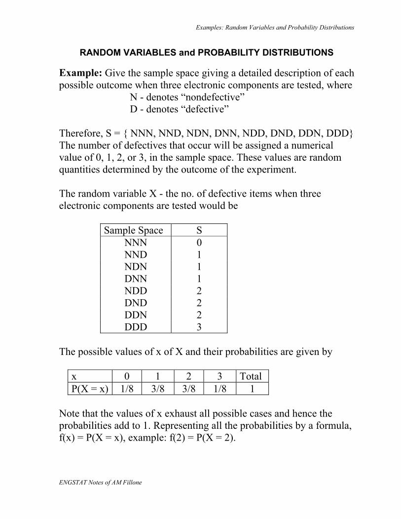
The set of ordered pair (x, f(x)) is called the probability function or probability distribution of the discrete random variable X. Example: Discrete probability distribution 11/60) A shipment of 7 television sets contains 2 defective sets. A hotel makes a random purchase of 3 of the sets. If X is the number of defective sets purchased by the hotel, find the probability distribution of X. Express the results graphically as a probability histogram. Sol’n: 2 5 0 3 10 2 f(0) = --------------- = --------- = ------- 7 35 7 3 2 5 1 2 20 4 f(1) = --------------- = --------- = ------- 7 35 7 3 2 5 2 1 5 1 f(2) = --------------- = --------- = ------- 7 35 7 3 Therefore, the probability distribution of x is

x 0 1 2 f(x) 2/7 4/7 1/7



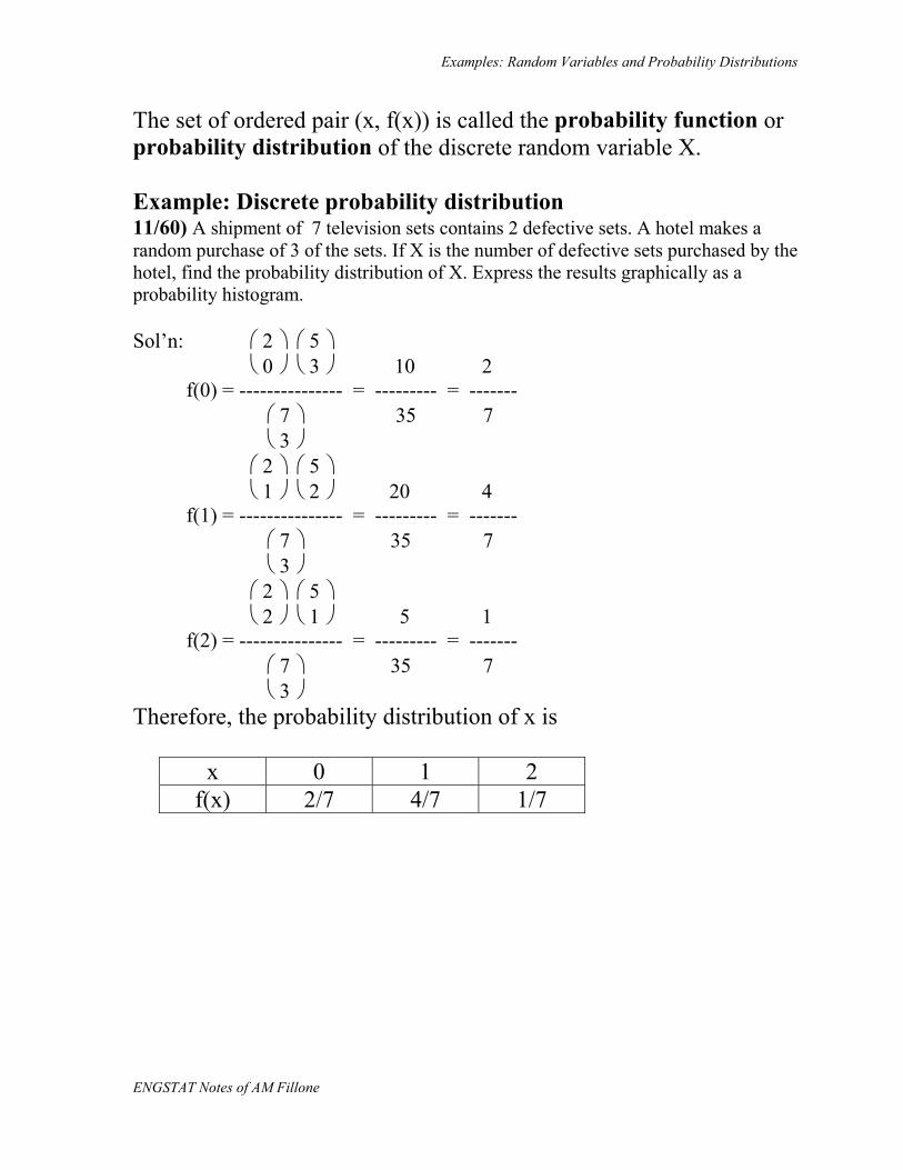
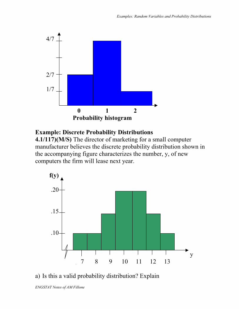
4/7 2/7 1/7 0 1 2 Probability histogram Example: Discrete Probability Distributions 4.1/117)(M/S) The director of marketing for a small computer manufacturer believes the discrete probability distribution shown in the accompanying figure characterizes the number, y, of new computers the firm will lease next year. f(y) .20 .15 .10 y 7 8 9 10 11 12 13 a) Is this a valid probability distribution? Explain



b) Display the probability distribution in tabular form. c) What is the probability that exactly 9 computers will be leased? d) What is the probability that fewer than 12 computers will be

leased? Sol’n: a) Yes b)

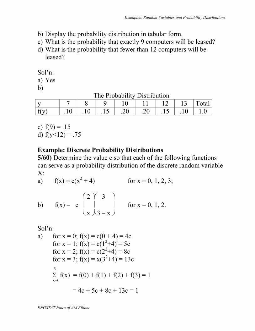
The Probability Distribution y 7 8 9 10 11 12 13 Totalf(y) .10 .10 .15 .20 .20 .15 .10 1.0 c) f(9) = .15 d) f(y<12) = .75 Example: Discrete Probability Distributions 5/60) Determine the value c so that each of the following functions can serve as a probability distribution of the discrete random variable X: a) f(x) = c(x2 + 4) for x = 0, 1, 2, 3; 2 3 b) f(x) = c for x = 0, 1, 2. x 3 – x Sol’n: a) for x = 0; f(x) = c(0 + 4) = 4c

for x = 1; f(x) = c(12+4) = 5c for x = 2; f(x) = c(22+4) = 8c for x = 3; f(x) = x(32+4) = 13c 3 Σ f(x) = f(0) + f(1) + f(2) + f(3) = 1 x=0

= 4c + 5c + 8c + 13c = 1



c = 1/30

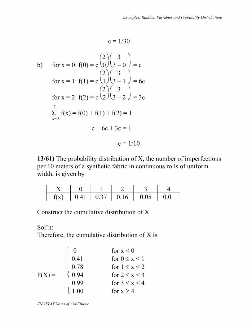
2 3 b) for x = 0: f(0) = c 0 3 – 0 = c 2 3 for x = 1: f(1) = c 1 3 – 1 = 6c 2 3 for x = 2: f(2) = c 2 3 – 2 = 3c 2

Σ f(x) = f(0) + f(1) + f(2) = 1 x=0

c + 6c + 3c = 1 c = 1/10 13/61) The probability distribution of X, the number of imperfections per 10 meters of a synthetic fabric in continuous rolls of uniform width, is given by

X 0 1 2 3 4 f(x) 0.41 0.37 0.16 0.05 0.01

Construct the cumulative distribution of X. Sol’n: Therefore, the cumulative distribution of X is

0 for x < 0 0.41 for 0 ≤ x < 1 0.78 for 1 ≤ x < 2 F(X) = 0.94 for 2 ≤ x < 3 0.99 for 3 ≤ x < 4 1.00 for x ≥ 4



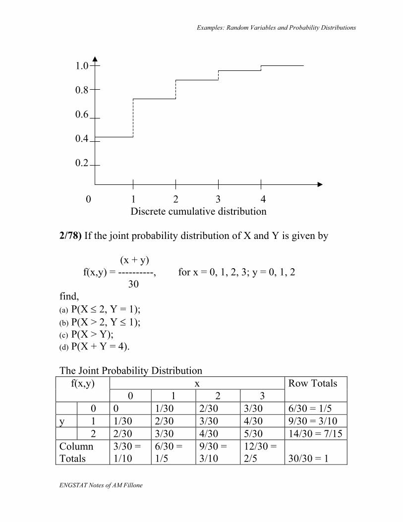
1.0 0.8 0.6 0.4 0.2 0 1 2 3 4 Discrete cumulative distribution 2/78) If the joint probability distribution of X and Y is given by (x + y) f(x,y) = ----------, for x = 0, 1, 2, 3; y = 0, 1, 2 30 find, (a) P(X ≤ 2, Y = 1); (b) P(X > 2, Y ≤ 1); (c) P(X > Y); (d) P(X + Y = 4). The Joint Probability Distribution

f(x,y) x Row Totals 0 1 2 3 0 0 1/30 2/30 3/30 6/30 = 1/5 y 1 1/30 2/30 3/30 4/30 9/30 = 3/10 2 2/30 3/30 4/30 5/30 14/30 = 7/15Column Totals

3/30 = 1/10

6/30 = 1/5

9/30 = 3/10

12/30 = 2/5

30/30 = 1



a) P(X ≤ 2, Y = 1) = f(0,1) + f(1,1) + f(2,1) =1/30 + 2/30 + 3/30 = 6/30

= 1/5 b) P(X > 2, Y ≤ 1) = f(3,0) + f(3,1) = 3/30 + 4/30

= 7/30 c) P(X > Y) = f(1,0) + f(2,0) + f(3,0) + f(2,1) + f(3,1) + f(3,2) = 1/30 + 2/30 + 3/30 + 3/30 + 4/30 + 5/30

= 18/30 = 3/5

d) P(X + Y = 4) = f(2,2) + f(3,1) = 4/30 + 4/30 = 8/30 = 4/15.

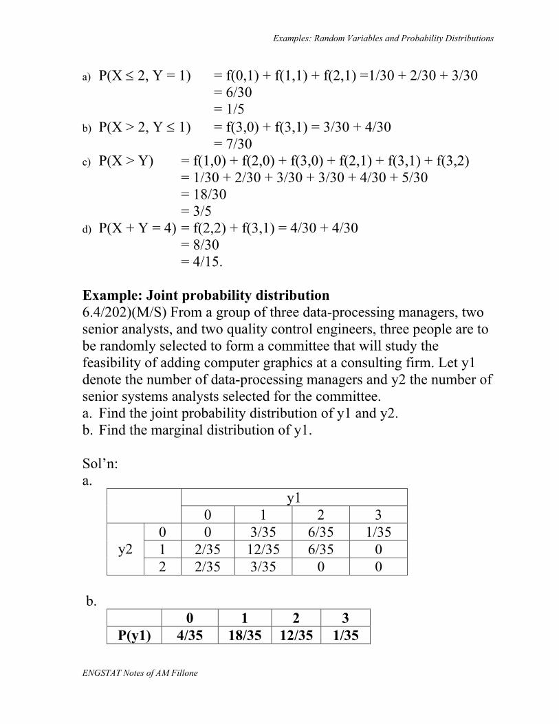
Example: Joint probability distribution 6.4/202)(M/S) From a group of three data-processing managers, two senior analysts, and two quality control engineers, three people are to be randomly selected to form a committee that will study the feasibility of adding computer graphics at a consulting firm. Let y1 denote the number of data-processing managers and y2 the number of senior systems analysts selected for the committee. a. Find the joint probability distribution of y1 and y2. b. Find the marginal distribution of y1. Sol’n: a.

y1 0 1 2 3

0 0 3/35 6/35 1/35 1 2/35 12/35 6/35 0

y2

2 2/35 3/35 0 0 b.

0 1 2 3 P(y1) 4/35 18/35 12/35 1/35



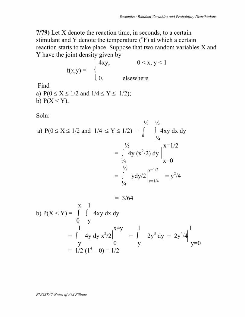
7/79) Let X denote the reaction time, in seconds, to a certain stimulant and Y denote the temperature (oF) at which a certain reaction starts to take place. Suppose that two random variables X and Y have the joint density given by 4xy, 0 < x, y < 1 f(x,y) = 0, elsewhere Find a) P(0 ≤ X ≤ 1/2 and 1/4 ≤ Y ≤ 1/2); b) P(X < Y). Soln: ½ ½ a) P(0 ≤ X ≤ 1/2 and 1/4 ≤ Y ≤ 1/2) = ∫ ∫ 4xy dx dy

0 ¼ ½ x=1/2

= ∫ 4y (x2/2) dy ¼ x=0 ½ y=1/2 = ∫ ydy/2 = y2/4

¼ y=1/4 = 3/64 x 1 b) P(X < Y) = ∫ ∫ 4xy dx dy 0 y 1 x=y 1 1 = ∫ 4y dy x2/2 = ∫ 2y3 dy = 2y4/4 y 0 y y=0 = 1/2 (14 – 0) = 1/2



Example: Independence 24/80) Determine whether the two random variables of Exercise 7 are dependent or independent. Sol’n: The joint density function is given as 4xy, 0 < x, y < 1 f(x,y) = 0, elsewhere 1 1 g(x) = ∫ 4xy dy = 4x [y2/2] = 2x [12 – 0] = 2x

0 0 1 1 h(y) = ∫ 4xy dx = 4y [x2/2] = 2y [12 – 0] = 2y 0 0 Hence,

f(x,y) = g(x)h(y), 0 < x,y < 1 4xy = (2x)(2y) 4xy = 4xy Therefore, x and y are independent. Example: Continuous probability distribution 17/61) A continuous random variable X that can assume values between x = 1 and x = 3 has a density function given by f(x) = 1/2. a) Show that the area under the curve is equal to 1. b) Find P(2 < X < 2.5). c) Find P(X ≤ 1.6).



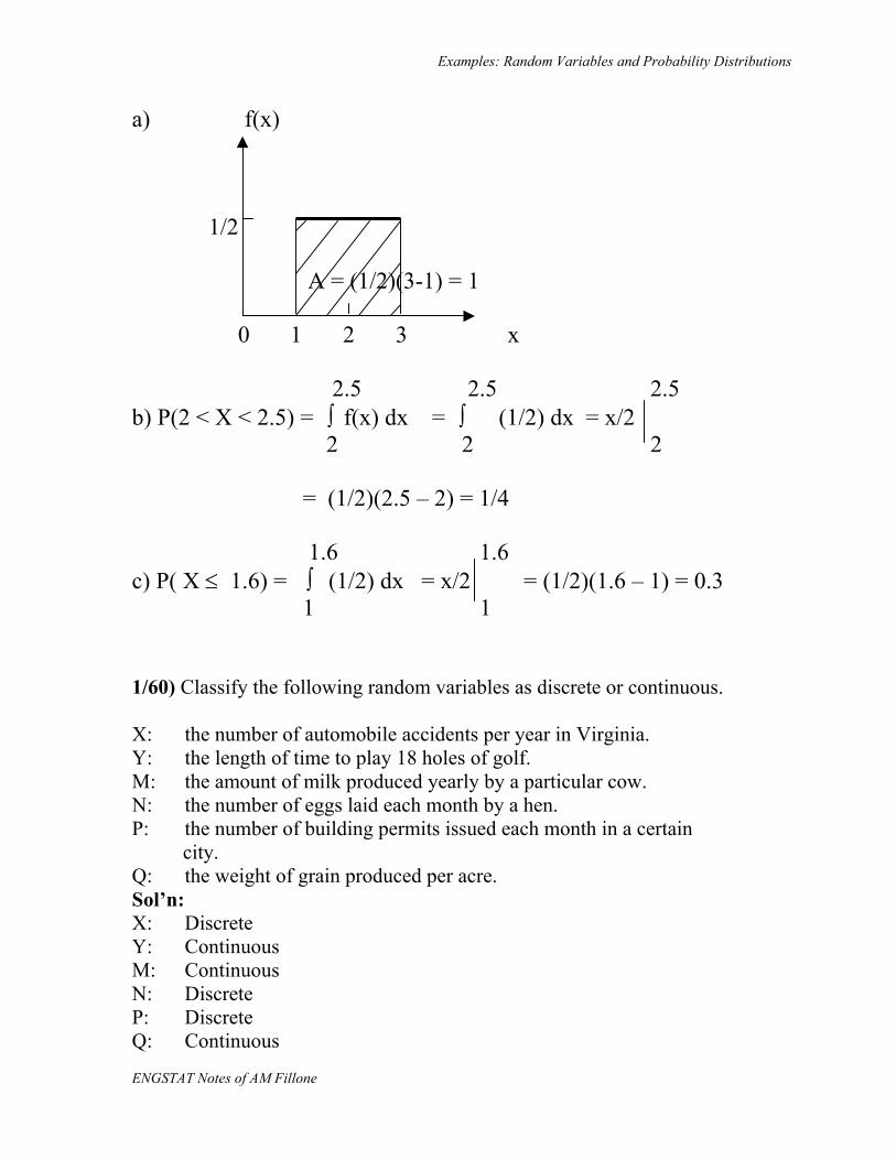
a) f(x) 1/2 A = (1/2)(3-1) = 1 0 1 2 3 x 2.5 2.5 2.5 b) P(2 < X < 2.5) = ∫ f(x) dx = ∫ (1/2) dx = x/2 2 2 2 = (1/2)(2.5 – 2) = 1/4 1.6 1.6 c) P( X ≤ 1.6) = ∫ (1/2) dx = x/2 = (1/2)(1.6 – 1) = 0.3 1 1 1/60) Classify the following random variables as discrete or continuous. X: the number of automobile accidents per year in Virginia. Y: the length of time to play 18 holes of golf. M: the amount of milk produced yearly by a particular cow. N: the number of eggs laid each month by a hen. P: the number of building permits issued each month in a certain city. Q: the weight of grain produced per acre. Sol’n: X: Discrete Y: Continuous M: Continuous N: Discrete P: Discrete Q: Continuous



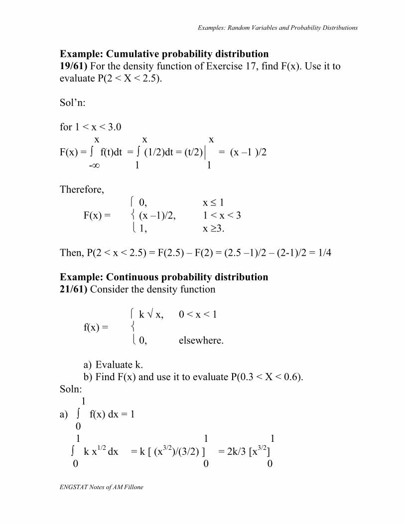
Example: Cumulative probability distribution 19/61) For the density function of Exercise 17, find F(x). Use it to evaluate P(2 < X < 2.5). Sol’n: for 1 < x < 3.0 x x x F(x) = ∫ f(t)dt = ∫ (1/2)dt = (t/2) = (x –1 )/2 -∞ 1 1 Therefore, 0, x ≤ 1 F(x) = (x –1)/2, 1 < x < 3 1, x ≥3. Then, P(2 < x < 2.5) = F(2.5) – F(2) = (2.5 –1)/2 – (2-1)/2 = 1/4 Example: Continuous probability distribution 21/61) Consider the density function k √ x, 0 < x < 1 f(x) = 0, elsewhere.

a) Evaluate k. b) Find F(x) and use it to evaluate P(0.3 < X < 0.6).

Soln: 1 a) ∫ f(x) dx = 1 0 1 1 1 ∫ k x1/2 dx = k [ (x3/2)/(3/2) ] = 2k/3 [x3/2] 0 0 0



2k/3 [13/2 – 0] = 1 k = 3/2 x b) F(X) = P (X ≤ x) = ∫ f(t) dt - ∝ x x x = ∫ (3/2)t1/2 dt = (3/2) t3/2 / (3/2) = t3/2 = x3/2 0 0 0

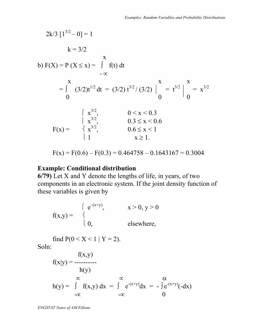
x3/2, 0 < x < 0.3 x3/2, 0.3 ≤ x < 0.6 F(x) = x3/2, 0.6 ≤ x < 1 1 x ≥ 1. F(x) = F(0.6) – F(0.3) = 0.464758 – 0.1643167 = 0.3004 Example: Conditional distribution 6/79) Let X and Y denote the lengths of life, in years, of two components in an electronic system. If the joint density function of these variables is given by e–(x+y), x > 0, y > 0

f(x,y) = 0, elsewhere, find P(0 < X < 1 | Y = 2). Soln: f(x,y) f(x|y) = ---------- h(y) ∝ ∝ α h(y) = ∫ f(x,y) dx = ∫ e-(x+y)dx = - ∫ e-(x+y)(-dx) -∝ -∝ 0



α = - e-(x +y) = - [e-(α+y) – e-y] 0 = e-y [ 1 – e-α] = e-y f(x,y) e-(x+y) e-xe-y

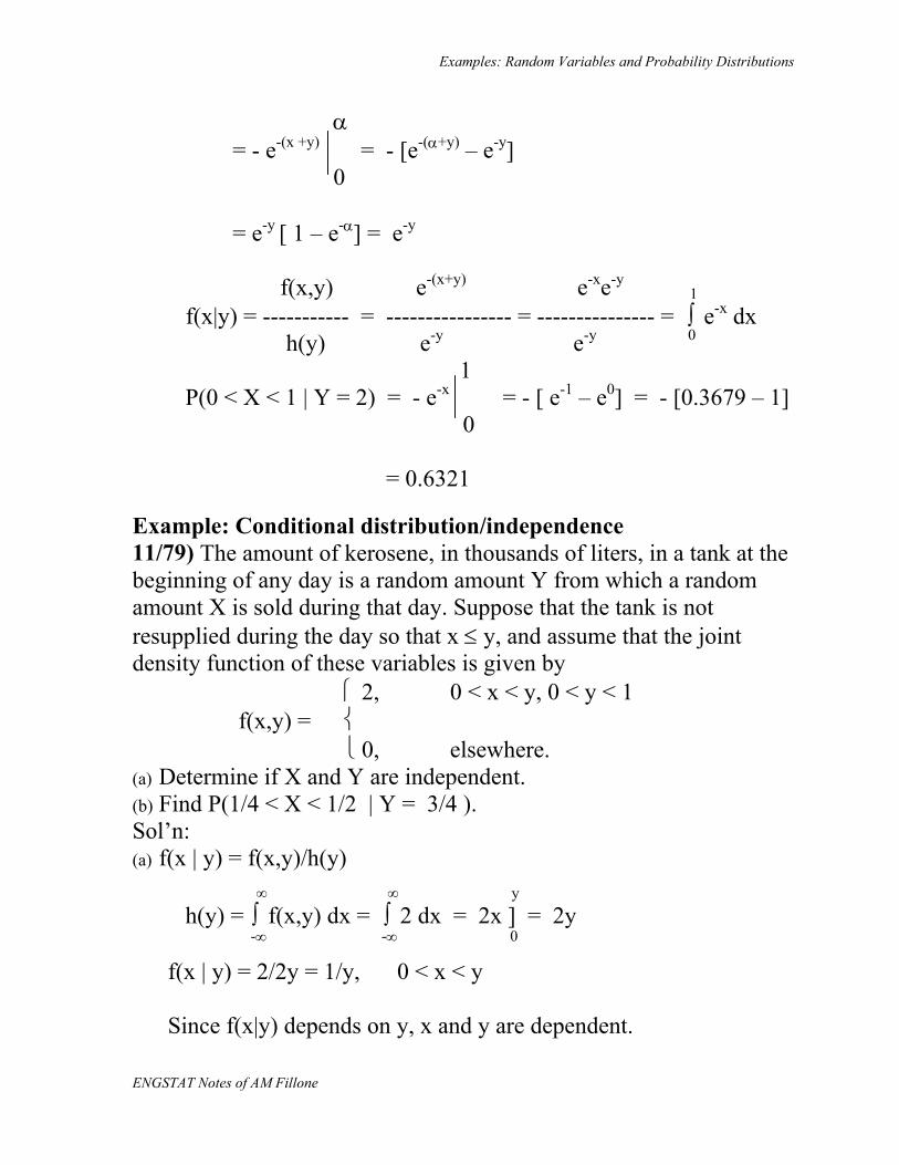
1 f(x|y) = ----------- = ---------------- = --------------- = ∫ e-x dx h(y) e-y e-y 0 1 P(0 < X < 1 | Y = 2) = - e-x = - [ e-1 – e0] = - [0.3679 – 1] 0

= 0.6321 Example: Conditional distribution/independence 11/79) The amount of kerosene, in thousands of liters, in a tank at the beginning of any day is a random amount Y from which a random amount X is sold during that day. Suppose that the tank is not resupplied during the day so that x ≤ y, and assume that the joint density function of these variables is given by

2, 0 < x < y, 0 < y < 1 f(x,y) = 0, elsewhere. (a) Determine if X and Y are independent. (b) Find P(1/4 < X < 1/2 | Y = 3/4 ). Sol’n: (a) f(x | y) = f(x,y)/h(y) ∞ ∞ y h(y) = ∫ f(x,y) dx = ∫ 2 dx = 2x ] = 2y -∞ -∞ 0 f(x | y) = 2/2y = 1/y, 0 < x < y Since f(x|y) depends on y, x and y are dependent.



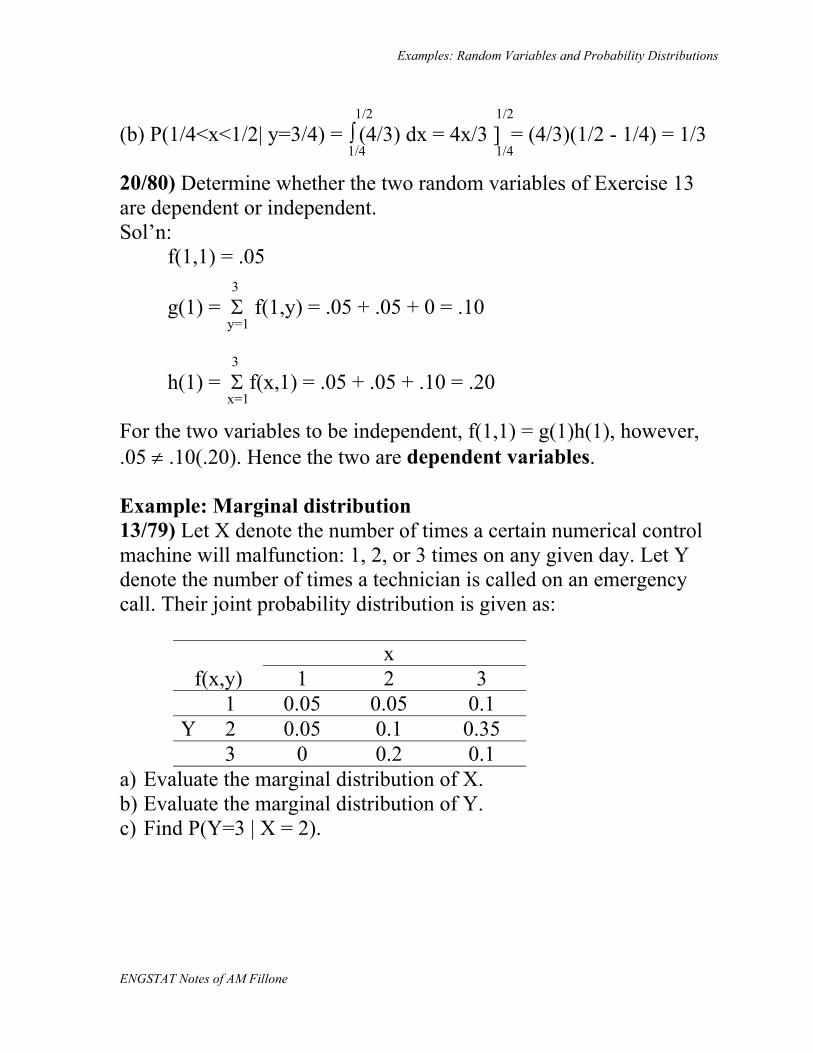
1/2 1/2 (b) P(1/4<x<1/2| y=3/4) = ∫ (4/3) dx = 4x/3 ] = (4/3)(1/2 - 1/4) = 1/3 1/4 1/4 20/80) Determine whether the two random variables of Exercise 13 are dependent or independent. Sol’n:

f(1,1) = .05 3

g(1) = Σ f(1,y) = .05 + .05 + 0 = .10 y=1

3 h(1) = Σ f(x,1) = .05 + .05 + .10 = .20 x=1

For the two variables to be independent, f(1,1) = g(1)h(1), however, .05 ≠ .10(.20). Hence the two are dependent variables. Example: Marginal distribution 13/79) Let X denote the number of times a certain numerical control machine will malfunction: 1, 2, or 3 times on any given day. Let Y denote the number of times a technician is called on an emergency call. Their joint probability distribution is given as:

x f(x,y) 1 2 3

1 0.05 0.05 0.1 Y 2 0.05 0.1 0.35 3 0 0.2 0.1

a) Evaluate the marginal distribution of X. b) Evaluate the marginal distribution of Y. c) Find P(Y=3 | X = 2).



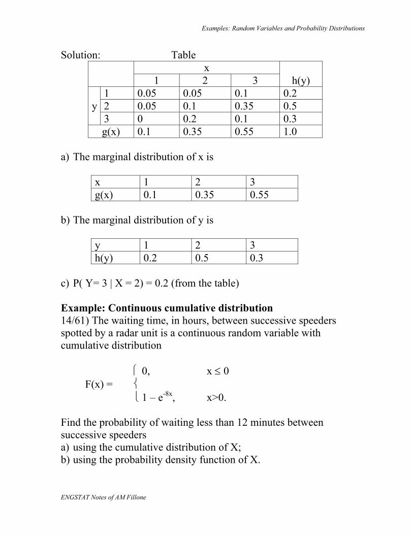
Solution: Table x 1 2 3 h(y) 1 0.05 0.05 0.1 0.2 y 2 0.05 0.1 0.35 0.5 3 0 0.2 0.1 0.3

g(x) 0.1 0.35 0.55 1.0 a) The marginal distribution of x is

x 1 2 3 g(x) 0.1 0.35 0.55

b) The marginal distribution of y is

y 1 2 3 h(y) 0.2 0.5 0.3

c) P( Y= 3 | X = 2) = 0.2 (from the table) Example: Continuous cumulative distribution 14/61) The waiting time, in hours, between successive speeders spotted by a radar unit is a continuous random variable with cumulative distribution 0, x ≤ 0 F(x) = 1 – e-8x, x>0. Find the probability of waiting less than 12 minutes between successive speeders a) using the cumulative distribution of X; b) using the probability density function of X.



Sol’n: 12 minutes = 0.2 hrs. 0 a) P(x < 0.2) = F(0.2) – F(0) = [1- e-8(.2)] – [1 – e-8(0)] = 0.7981 b) f(x) = dF(x)/dx = (1-e-8x)(-8dx)/dx = (-8)( 1-e-8x) 0.2 0.2 P(0 < x< 0.2) = ∫ (-8)( 1-e-8x) dx = [1-e-8x] = 0.7981 0 0

Documents

Stat