Embed Size (px)
Citation preview
State-Aggregation Algorithms for Learning
Probabilistic Models for Robot Control
Daniel Nikovski
CMU-RI-TR-02-04
Submitted in partial fulfillment
of the requirements for the degree of
Doctor of Philosophy in Robotics
The Robotics Institute
Carnegie Mellon University
Pittsburgh, PA 15213
Thesis Committee:
Illah Nourbakhsh, Chair
Tom Mitchell
Sebastian Thrun
Benjamin Kuipers
c 2002 Carnegie Mellon University

1
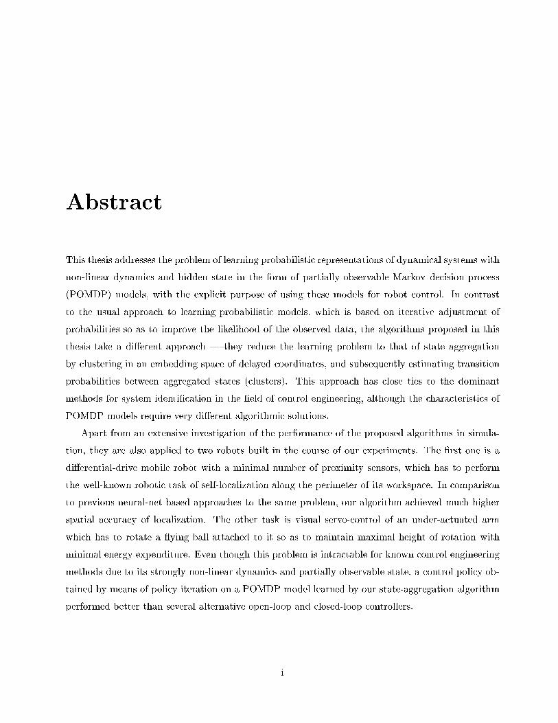
Abstract
This thesis addresses the problem of learning probabilistic representations of dynamical systems with
non-linear dynamics and hidden state in the form of partially observable Markov decision process
(POMDP) models, with the explicit purpose of using these models for robot control. In contrast
to the usual approach to learning probabilistic models, which is based on iterative adjustment of
probabilities so as to improve the likelihood of the observed data, the algorithms proposed in this
thesis take a di�erent approach | they reduce the learning problem to that of state aggregation
by clustering in an embedding space of delayed coordinates, and subsequently estimating transition
probabilities between aggregated states (clusters). This approach has close ties to the dominant
methods for system identi�cation in the �eld of control engineering, although the characteristics of
POMDP models require very di�erent algorithmic solutions.
Apart from an extensive investigation of the performance of the proposed algorithms in simula-
tion, they are also applied to two robots built in the course of our experiments. The �rst one is a
di�erential-drive mobile robot with a minimal number of proximity sensors, which has to perform
the well-known robotic task of self-localization along the perimeter of its workspace. In comparison
to previous neural-net based approaches to the same problem, our algorithm achieved much higher
spatial accuracy of localization. The other task is visual servo-control of an under-actuated arm
which has to rotate a ying ball attached to it so as to maintain maximal height of rotation with
minimal energy expenditure. Even though this problem is intractable for known control engineering
methods due to its strongly non-linear dynamics and partially observable state, a control policy ob-
tained by means of policy iteration on a POMDP model learned by our state-aggregation algorithm
performed better than several alternative open-loop and closed-loop controllers.
i
Acknowledgments
First and foremost, I would like to thank the members of my thesis committee for all of their time and
e�ort spent helping me complete this thesis. I am greatly indebted to my thesis supervisor, Professor
Illah Nourbakhsh, for his constant support, advice, encouragement, and inspiration | working with
him has been a real pleasure. Many thanks are also due to Professor Tom Mitchell, who not only
led my initial research and patiently introduced me to the �eld of learning robots, but also stayed
on my thesis committee and made many helpful suggestions on the thesis. I am very grateful to
Professor Sebastian Thrun, too, who was the �rst to suggest that I consider the problem of learning
POMDP models, and also closely monitored my progress and provided many signi�cant suggestions
and critiques over the years. The external committee member, Professor Benjamin Kuipers, also
contributed greatly by critically evaluating my thesis with respect to other learning methods in
robotics.
The Robotics Institute at Carnegie Mellon was not only a provider of administrative, �nancial,
and logistical support, but also a great place to work, study, and enjoy academia. I appreciate very
much the great camaraderie among the students in the Robotics PhD Program, which made the
years spent at Carnegie Mellon so enjoyable and ful�lling.
Finally, I would like to thank my parents for trusting me that I knew what I was doing halfway
around the globe, and also my wonderful friends in Pittsburgh and elsewhere, too numerous to list
here, for keeping me sane during all these years, and helping me keep a sound perspective on life and
research.
ii
Contents
1 Introduction 1
1.1 Motivation . . . . . . . . . . . . . . . . . . . . . . . . . . . . . . . . . . . . . . . . . . 1
1.2 Problem Statement . . . . . . . . . . . . . . . . . . . . . . . . . . . . . . . . . . . . . . 4
1.3 Scope and Limitations of Research . . . . . . . . . . . . . . . . . . . . . . . . . . . . . 6
1.4 Overview . . . . . . . . . . . . . . . . . . . . . . . . . . . . . . . . . . . . . . . . . . . 7
1.5 Summary of Main Results and Contributions . . . . . . . . . . . . . . . . . . . . . . . 9
2 Reasoning, Planning, and Learning in Robotics 12
2.1 General Requirements for Autonomous Robots . . . . . . . . . . . . . . . . . . . . . . 12
2.2 Representation . . . . . . . . . . . . . . . . . . . . . . . . . . . . . . . . . . . . . . . . 13
2.3 Reasoning . . . . . . . . . . . . . . . . . . . . . . . . . . . . . . . . . . . . . . . . . . . 23
2.4 Learning . . . . . . . . . . . . . . . . . . . . . . . . . . . . . . . . . . . . . . . . . . . . 27
2.5 Planning and Control . . . . . . . . . . . . . . . . . . . . . . . . . . . . . . . . . . . . 34
3 System Representation, Reasoning and Planning with POMDPs 41
3.1 De�nition of POMDPs . . . . . . . . . . . . . . . . . . . . . . . . . . . . . . . . . . . . 41
3.2 Reasoning by Means of Belief Updating . . . . . . . . . . . . . . . . . . . . . . . . . . 43
3.3 Planning with POMDPs . . . . . . . . . . . . . . . . . . . . . . . . . . . . . . . . . . . 43
4 Learning POMDP Models by Iterative Adjustment of Probabilities 48
4.1 Steepest Gradient Ascent (SGA) in Likelihood . . . . . . . . . . . . . . . . . . . . . . 49
4.2 Baum-Welch . . . . . . . . . . . . . . . . . . . . . . . . . . . . . . . . . . . . . . . . . 49
4.3 Experimental Comparison between BW and SGA . . . . . . . . . . . . . . . . . . . . . 51
iii
CONTENTS iv
4.4 Learning POMDPs with Continuous Observations . . . . . . . . . . . . . . . . . . . . 54
4.4.1 Clustering of Observations . . . . . . . . . . . . . . . . . . . . . . . . . . . . . . 56
5 Learning POMDP Models by State Aggregation 61
5.1 Best-First Model Merging . . . . . . . . . . . . . . . . . . . . . . . . . . . . . . . . . . 61
5.2 State Merging by Trajectory Clustering . . . . . . . . . . . . . . . . . . . . . . . . . . 64
5.3 Experimental Comparison between BW, SGA, BFMM, and SMTC on Benchmark
POMDP Models . . . . . . . . . . . . . . . . . . . . . . . . . . . . . . . . . . . . . . . 68
5.4 Experimental Comparison between BW, SGA, BFMM, and SMTC on Restricted Mo-
bile Robot Navigation . . . . . . . . . . . . . . . . . . . . . . . . . . . . . . . . . . . . 72
6 Constrained Trajectory Clustering for Mobile Robot Localization 82
6.1 Space Exploration Policies for Mobile Robots . . . . . . . . . . . . . . . . . . . . . . . 82
6.2 Experimental Task . . . . . . . . . . . . . . . . . . . . . . . . . . . . . . . . . . . . . . 84
6.3 Experimental Robot and Low-Level Control . . . . . . . . . . . . . . . . . . . . . . . . 85
6.4 Learning an HMM by State Merging . . . . . . . . . . . . . . . . . . . . . . . . . . . . 89
6.5 Learning an HMM with Discrete Emission Distributions . . . . . . . . . . . . . . . . . 91
6.6 Experimental Environment and Results . . . . . . . . . . . . . . . . . . . . . . . . . . 93
6.7 Learning an HMM with Circular Emission Distributions . . . . . . . . . . . . . . . . . 99
6.8 Experimental Environment and Results . . . . . . . . . . . . . . . . . . . . . . . . . . 104
6.9 Extensions to Full Planar Navigation . . . . . . . . . . . . . . . . . . . . . . . . . . . . 110
7 Learning POMDPs by Clustering Trajectory Features 112
7.1 Experimental Manipulator and Task . . . . . . . . . . . . . . . . . . . . . . . . . . . . 112
7.2 Analysis of a Harmonically Driven Spherical Pendulum . . . . . . . . . . . . . . . . . . 116
7.3 State Estimation and Control by Delayed-Coordinate Embedding . . . . . . . . . . . . 121
7.4 Learning a FOMDP Model by Delayed-Coordinate Embedding . . . . . . . . . . . . . 126
7.5 Experimental Results for Circles in Joint Space . . . . . . . . . . . . . . . . . . . . . . 129
7.6 Experimental Results for Circles in Cartesian Space . . . . . . . . . . . . . . . . . . . 135
8 Conclusions and Future Research 142
A Derivation of the Equations of Motion of the Arm 148
List of Figures
3.1 Diagram of a dynamic Bayesian network . . . . . . . . . . . . . . . . . . . . . . . . . . 42
4.1 Comparison between SGA and Baum-Welch . . . . . . . . . . . . . . . . . . . . . . . . 52
4.2 Parameter convergence . . . . . . . . . . . . . . . . . . . . . . . . . . . . . . . . . . . . 53
4.3 Convergence of Baum-Welch for the action models of actions a1 and a2. . . . . . . . . 54
4.4 Learning a two-state POMDP with two observations and two actions . . . . . . . . . . 59
4.5 Experimental world for k-means clustering of infrared readings. . . . . . . . . . . . . . 60
5.1 Test worlds Easy4, Hard4, and Harder4. . . . . . . . . . . . . . . . . . . . . . . . . . . 69
5.2 Experimental world for learning and planning in a Nomad simulator. . . . . . . . . . . 76
6.1 The mobile robot Mr. Spoon . . . . . . . . . . . . . . . . . . . . . . . . . . . . . . . . 86
6.2 Lower deck of Mr. Spoon . . . . . . . . . . . . . . . . . . . . . . . . . . . . . . . . . . 87
6.3 Experimental world for Mr. Spoon . . . . . . . . . . . . . . . . . . . . . . . . . . . . . 94
6.4 Training portion of the exploration trace. . . . . . . . . . . . . . . . . . . . . . . . . . 95
6.5 Mismatch (inter-trajectory distance) as a function of the period . . . . . . . . . . . . . 96
6.6 Experimental results for localization. . . . . . . . . . . . . . . . . . . . . . . . . . . . . 98
6.7 Probability density function of the von Mises distribution. . . . . . . . . . . . . . . . . 101
6.8 Estimation of the preferred direction � from observed direction samples. . . . . . . . . 102
6.9 Second experimental world for Mr. Spoon . . . . . . . . . . . . . . . . . . . . . . . . . 105
6.10 Training and testing traces. . . . . . . . . . . . . . . . . . . . . . . . . . . . . . . . . . 106
6.11 Mismatch (inter-trajectory distance) as a function of the period . . . . . . . . . . . . . 107
6.12 Self-localization from time 0. . . . . . . . . . . . . . . . . . . . . . . . . . . . . . . . . 108
6.13 Self-localization from time 100. . . . . . . . . . . . . . . . . . . . . . . . . . . . . . . . 109
v
LIST OF FIGURES vi
6.14 Self-localization from time 300. . . . . . . . . . . . . . . . . . . . . . . . . . . . . . . . 110
6.15 Self-localization from time 800. . . . . . . . . . . . . . . . . . . . . . . . . . . . . . . . 111
7.1 Experimental arm in resting state. . . . . . . . . . . . . . . . . . . . . . . . . . . . . . 113
7.2 Parametrization of a spherical pendulum with rotating support. . . . . . . . . . . . . . 118
7.3 Numerically integrated equations of motion of the arm. . . . . . . . . . . . . . . . . . 119
7.4 Attractor of the dynamical system of the arm. . . . . . . . . . . . . . . . . . . . . . . . 120
7.5 Periodic variation of the height of the ball for r = 120mm. . . . . . . . . . . . . . . . . 121
7.6 Dependency of the average height on r and !=!0 . . . . . . . . . . . . . . . . . . . . . 122
7.7 Observed transitions for ellipsoidal motion in joint space. . . . . . . . . . . . . . . . . 131
7.8 Code book resulting from the application of LVQ to a 16-dimensional coordinate
embedding. . . . . . . . . . . . . . . . . . . . . . . . . . . . . . . . . . . . . . . . . . . 132
7.9 Performance under varying cost multipliers for several policies. . . . . . . . . . . . . . 134
7.10 Control signal and measured height of the ball under the computed optimal policy for
� = 1. In the upper plot, the dependent variable is 1 for action a and 0 for action b. . 135
7.11 Dependency of the average height of stable orbiting on r . . . . . . . . . . . . . . . . . 136
7.12 Observed transitions for circular motion in Cartesian space. . . . . . . . . . . . . . . . 137
7.13 Performance vs. cost multiplier for 17 policies. . . . . . . . . . . . . . . . . . . . . . . 140

List of Tables
5.1 Steepest gradient ascent in the log-likelihood of observations. . . . . . . . . . . . . . . 73
5.2 Baum-Welch. . . . . . . . . . . . . . . . . . . . . . . . . . . . . . . . . . . . . . . . . . 73
5.3 Best-�rst model merging. . . . . . . . . . . . . . . . . . . . . . . . . . . . . . . . . . . 74
5.4 State merging by trajectory clustering. . . . . . . . . . . . . . . . . . . . . . . . . . . . 74
5.5 Planning by means of the true POMDP models. . . . . . . . . . . . . . . . . . . . . . 75
5.6 Results for four learning methods and �ve planners. . . . . . . . . . . . . . . . . . . . 78
6.1 Low-level command parameters for wall-following behavior. . . . . . . . . . . . . . . . 89
7.1 Results for three values of the cost multiplier �. . . . . . . . . . . . . . . . . . . . . . . 133
vii

LIST OF TABLES viii
Chapter 1
Introduction
1.1 Motivation
Deliberative reasoning and decision making are two of the main faculties which distinguish a robot
from a simple automaton designed to perform a single function. The common way to achieve these
faculties is by endowing the robot with a model of its environment, which can be used to reason
about the state of the world, make plans to achieve objectives, and track the execution of such plans.
The availability of world models allows an intelligent robot to serve multiple purposes and follow
multiple objectives, rather than simply following a �xed routine.
The general approach in robotics (and the whole area of automatic control in general) is to use
mathematical models which re ect the evolution of the state of a robot as a result of its actions,
and describe the relationship between its state and the percepts observed directly by its sensors. In
the vast majority of cases, such models are provided by a human designer, which often entails high
costs and signi�cant e�ort. Our principal objective is to propose machine learning methods and
algorithms which automate the process of model building, thus reducing or completely eliminating
the work performed by human designers. This work expense is one of the major blocks to a more
widespread use of robotics, and eliminating it would signi�cantly reduce the cost of developing and
deploying robots. Furthermore, it is desirable that these algorithms be able to learn models from data
obtained autonomously by the robot, rather than data resulting from extensive human instruction
or supervision.
One of the principal directions to creating more autonomous robotic systems is to provide robots
1
CHAPTER 1. INTRODUCTION 2
with means to autonomously acquire world models, learning from their own experience, just like
living organisms learn to deal with their environment. A large number of machine learning algo-
rithms have been applied to robotic tasks, and several common representational and decision making
paradigms from the wider �elds of Arti�cial Intelligence (AI) and control systems engineering have
been explored, among which are �rst-order logic, linear state-space models, neural networks, fuzzy
logic, graphical models, etc. Since the �eld of robotics poses speci�c challenges and requirements,
most notably high uncertainty in sensing and action, and partial observability of system state, some
of these paradigms are better suited to learning problems in robotics than others.
A paradigm, especially applicable to reasoning, planning, and learning tasks in robotics, is that of
probabilistic decision models, also known as Markov decision problem (MDP) models. Due to their
�rm foundation in probability and decision theory, MDP models are well suited to handle uncertainty,
sequential decision making, and limited observability, with reasonable computational eÆciency. As
a result, the application of MDP models and probabilistic methods to robotic problems has gained
signi�cant popularity. Given the high utility of probabilistic models in robotics, it is highly desirable
to develop machine learning algorithms, which can learn such models from training data that can be
acquired autonomously by a mobile robot.
It should be noted, however, that the problem of learning MDP models di�ers signi�cantly from
other probabilistic machine learning algorithms in terms of the �nal models these algorithms learn.
There exist many algorithms that use probabilistic methods to learn models, but these models
themselves are geometric. For example, many computer vision algorithms are probabilistic, but still
the �nal models they extract are mostly 3D geometric descriptions of the observed environment.
Similarly, many mobile robots employ probabilistic techniques to acquire maps, but these maps
are essentially geometric models. While acquiring such geometric models is certainly useful, and
the extensive human experience with such models can be leveraged so that they can be used very
eÆciently, there are many robots and robotic tasks for which the acquisition of such models can be
very hard, expensive, or even completely impossible.
Consider, for example, a mobile robot which has no internal odometry and only a limited number
of proximity sensors that do not allow a geometric map to be built. Or a walking robot which would
usually have very poor built-in odometry by construction, unless expensive inertial navigation sensors
are used. Another example is a camera which is not calibrated and/or has signi�cant nonlinear
distortions, so that its viewing transformation is not known or very hard to obtain. Furthermore, if
CHAPTER 1. INTRODUCTION 3
a single camera is used, determining the 3D structure of a scene is an ill-posed problem under most
practical circumstances, for example when the camera is stationary with respect to the scene and no
systematic change in lighting is performed.
When confronted by such problems, robot designers usually resort to adding more and/or better
sensors | synchro-drives for better odometry, multiple complete rings of proximity sensors, Global
Positioning System (GPS) sensors, triangulation beacons, multiple cameras with precise calibration
and optics, etc. Arguably, this is not the path to simpler, cheaper, and more maintenance-free
robots | if reducing costs by eliminating designer e�ort is desirable, so is reducing costs by using
fewer, simpler, and cheaper sensors. Accordingly, another motivation for the presented work has
been the need for probabilistic learning algorithms which can work on simple robots whose sensors
do not allow geometric models to be built. That this is possible is evident from the operation of
living organisms which negotiate perfectly well their environments, typically without any built-in
odometry or precisely calibrated sensors.
A third motivation for exploring algorithms for learning MDP models stems from the fact that
the state of an MDP model is represented as a set of discrete variables, while the state of the system
that model represents is usually continuous. Since the algorithms we investigate de�ne autonomously
discrete internal states of a model in terms of external sensory observations, they are a solution to
the state-grounding problem, which is a special case of the symbol-grounding problem identi�ed as
one of the fundamental research problems in arti�cial intelligence (AI) (Harnad, 1990). The main
question within the symbol-grounding problem is how entities internal to the reasoning apparatus of
an intelligent being (such as locations, paths, or high-level cognitive concepts) come into existence,
when the immediately observable percepts consist only of sensory patterns of external in uences (such
as light, sound, pressure, temperature, etc.), which have no intrinsic meaning to an organism or a
robot. The learned states provide a basic substrate of internal objects, upon which higher hierarchies
of cognitive concepts can be built, and thus provide the interface between the material world and
immaterial cognition. We believe that explaining how this substrate emerges autonomously is one
of the key issues in understanding how mind emerges from matter.
CHAPTER 1. INTRODUCTION 4
1.2 Problem Statement
The main research problem we are addressing in this thesis is the autonomous acquisition of proba-
bilistic models for the purposes of reasoning, planning, and control in robotic agents. By autonomous
acquisition of models we mean learning such models entirely from observation data, without prior
knowledge about the particular environment the robot is operating in. We are considering the set-
ting where the robot initially follows an exploration control policy, trying di�erent actions in many
situations, while simultaneously recording its sensory readings and the attempted actions in an obser-
vation/action sequence (execution trace). There is only one exploration stage, after which the robot
learns a model that explains (models) the execution trace as best as possible, hence the learning
algorithms build internal models using only such execution traces, without using any intermediate
learned models in order to guide exploration and accumulate more execution traces.
Furthermore, the learning algorithm builds a model without a prior notion of what constitutes
the state of the robot and the world. It is the job of the learning algorithm to de�ne such states so as
to model correctly the data in the execution trace, and also maximize the accuracy of predicting the
future evolution of the world, as well as successful achievement of its goals. The practical signi�cance
of such algorithms is multifold:
1. The controlled systems operate autonomously and thus save time and e�ort for system design-
ers.
2. The learned models can be reused when the control objectives change. This is in contrast to
model-free algorithms for optimal control, which would have to explore the system again in
such cases.
3. The learned models de�ne a set of primitive states by grounding them in percepts, thus provid-
ing a substrate for higher-level reasoning, planning, and learning algorithms. In this way, the
learning algorithms are a step towards the solution of the general symbol-grounding problem.
Various kinds of dynamic systems are employed in the �eld of robotics and automatic control, and
we limit our attention to a speci�c class of such systems. We are interested in non-linear systems that
have a signi�cant degree of uncertainty, and are characterized by very large or in�nite state spaces.
The performance criterion that a controller for these systems should optimize involves a sequence of
decision (control) steps, rather than a single step.
CHAPTER 1. INTRODUCTION 5
These systems have hidden state, i.e., the current state of the system cannot be identi�ed un-
ambiguously only by using the current sensor readings. However, these systems are assumed to be
observable in the control-theory sense of this term, i.e., an observer for their state can be built,
possibly using sequences of past percepts. The systems considered are of �nite dimension, which
means that the current system state can be identi�ed by considering a long enough (but still �nite)
sequence of past observations. Their state itself is continuous and hence their state spaces are of
in�nite size, which prohibits the use of known decision theoretic algorithms, such as policy and value
iteration that work only on discrete state spaces of low cardinality.
The restrictions we impose on the class of systems addressed by our algorithms are as follows:
1. The system is controlled by actions from a discrete set. Even though this excludes most dynamic
systems with continuous controls, such systems can be handled by limiting the controls available
to the controller to a small, carefully designed, discrete subset of all possible controls. This
corresponds to the common practice in algorithms for motion planning (Latombe, 1991).
2. The state space of the controlled system can be explored by means of a pre-speci�ed exploration
policy, i.e., the neighborhood of each state of the system can be reached by following the
exploration policy. In particular, when the performance criterion to be optimized by the
system controller includes reaching a speci�c goal state, this state should be reachable by the
exploration policy.
3. The system dynamics are stationary, i.e., the system dynamics do not change between the time
an execution trace is collected by following an exploration policy, and the time the system is to
be controlled by a controller, derived by means of learning a probabilistic model of the system
from this execution trace.
Examples from the class of dynamic systems under consideration include:
1. Mobile robots which have to reach a particular goal location in their workspace while minimizing
the traveled distance to that location. The set of actions available to the robot are limited to
a �nite set of rotations and translations, or more complicated, but still �xed behaviors. Most
mobile robot navigation problems can be formulated in this way (Latombe, 1991).
2. Manipulators which have to reach a goal con�guration, and are allowed at each control step to
move their joints by a small number of possible displacements. Other dynamic manipulation
CHAPTER 1. INTRODUCTION 6
tasks can be formulated this way too, such as juggling balls, moving loads to a goal location
by a crane so as to minimize the swing of the load, etc.
1.3 Scope and Limitations of Research
Even though the robots and robotic tasks considered in our experiments cover a large class of
systems and tasks in robotics and automatic control, they are not applicable to the most general
formulation of an optimal control task, where the learned model has continuous control variables.
When the controls are continuous, most of the well-known POMDP planning algorithms are not
directly applicable, and instead the Hamilton-Jacobi-Bellman (HJB) equations from optimal control
have to be applied. Since solving the HJB equations for an arbitrary non-linear system, even when its
dynamics are completely known, is still an unsolved problem (Stengel, 1994), there is no immediate
bene�t in developing algorithms for identifying models of such systems from observations.
For the speci�c problem of mobile robot navigation, we are limiting our attention to inexpensive
robots, which have only a small number of sensors and lack on-board odometry. There exist other
algorithms for learning models for mobile robot navigation by larger robots which have a complete
ring of sonars and/or infrared proximity sensors, as well as relatively precise odometric readings
from wheel encoders (Lu & Milios, 1997; Thrun et al., 1998b; Thrun et al., 1998c). Such algorithms
typically build a map of the environment in the form of a global occupancy grid, obtained by merging
local occupancy grids. The methods we propose are not meant for such robots, and are not meant
to compete with these algorithms. Conversely, these map-building algorithms are generally not
applicable to the class of robots we are considering.
The algorithms proposed in this thesis derive descriptions of the structure and dynamics of con-
tinuous worlds in terms of discrete models, thus implicitly discretizing continuous variables into
discrete ones. A similarly interesting and important problem is the discretization of naturally con-
tinuous controls, such as torques, directions, and velocities, into discrete actions. This thesis does
not deal with this problem | instead, we assume the availability of a small set of prede�ned actions,
whose combined application allows for a reasonably complete exploration of the world. The nature
and number of these actions depends on the problem considered. This corresponds to the general
practice in the �eld of robot motion planning.
A related question, which this thesis does not address as a research problem, is how to explore
CHAPTER 1. INTRODUCTION 7
optimally unknown worlds without knowledge of the exact coordinates of the robot. Even when such
knowledge is available, complete exploratory coverage of unknown spaces is not a trivial problem
and is still an area of active research (Choset, 2001). The algorithms in this thesis use several known
heuristic strategies which, although giving no guarantee for complete coverage, have been shown to
work well in practice.
1.4 Overview
The algorithms we propose build probabilistic models which are �rmly founded in probability theory.
Since probabilistic models are only one of a plethora of representations explored in AI, in Chapter 2
we review the state of the art in representations commonly used in AI, along with their associated
reasoning and planning algorithms. The objective of this review is not to compare the relative merits
of these methods within the whole �eld of AI, but to identify suitable representational, reasoning,
and planning schemes for the concrete problem of learning internal models which will subsequently
be used by robots in their reasoning and planning. In this chapter we argue that discrete probabilistic
models in the form of POMDPs are especially well suited to this purpose.
Chapter 3 describes the mathematical theory of POMDPs. This chapter also describes in detail
the existing relevant algorithms for reasoning and planning with POMDPs, which we use on the
models learned by our algorithms without substantial modi�cations.
The experimental tasks, robots, and their environments are presented in Chapters 4, 5, 6, and 7,
along with concrete research questions which allow quanti�able experimental results to be obtained.
These robots and environments include both navigation tasks on mobile robots, as well as manipu-
lation tasks on stationary robots. Some of the results have been performed in simulation, and others
on real robots that we have built in the course of our experiments. Various robotic sensors have been
used in these tasks, such as infrared proximity sensors, magnetic compasses, and monocular color
vision, in an e�ort to perform experiments in a wide and representative class of settings used in the
�eld of robotics.
Chapter 4 explores two traditional and widely used algorithms for learning probabilistic models
(Baum-Welch and steepest ascent in likelihood), and investigates experimentally their applicability
to recovering POMDPs, whose structure and probabilities are known in advance, with the explicit
CHAPTER 1. INTRODUCTION 8
purpose of using the learned models to plan optimal policies. Two severe limitations of these al-
gorithms are identi�ed: �rst, the abundance of shallow local maxima in model likelihood which
usually results in useless learned models, and second, the especially poor recovery of probabilities
between hidden nodes. Since approximate POMDP planning algorithms rely heavily on these prob-
abilities, the chapter concludes that the known traditional algorithms present very poor solutions to
the research problem considered in this thesis.
Chapter 5 explores an alternative approach to learning probabilistic models with hidden state
and proposes a novel algorithm (SMTC), which learns POMDPs by merging trajectories of percepts,
rather than the usual approach of iteratively adjusting probabilities so as to maximize data likelihood,
and exhaustively searching the space of all model structures. This algorithm is subjected to an
experimental comparison with three other algorithms| the two considered in Chapter 4, and another
state-merging algorithm (Best-First Model Merging). The comparison itself is in two parts: the �rst
part is on fourteen test POMDPs, chosen so as to be representative of the models which might
correspond to various robotic environments, and the second part considers a simulated mobile robot
environment using a commercial Nomad 150 simulator. The experimental comparison shows that the
novel algorithm compares favorably to the previously known learning algorithms, and its advantages
are statistically signi�cant.
Chapter 6 investigates the approach to learning POMDPs by means of state merging by trajectory
clustering on an experimental mobile robot built during the course of the experiments. This chapter
demonstrates that the proposed algorithm, unlike others, can exploit very eÆciently the constraints
of the exploration policy in order to perform very fast learning of a probabilistic model with high
spatial resolution, which can be used for mobile robot localization with high accuracy. Because of
the high eÆciency of the algorithm, it can be done completely on board the robot, unlike the much
slower performance of other known learning algorithms.
Chapter 7 explores further the approach to learning POMDPs by means of state merging, by
modifying the algorithm to cluster not raw trajectories, but features derived from these trajectories.
Since these features are numerical, the e�ect of clustering them instead of trajectories of percepts
is that eÆcient algorithms for clustering metric data can be used. The algorithm is applied to a
manipulation task on another robot built in the course of the experiments | a robotic arm with
two actuated and four unactuated degrees of freedom, which is equivalent to a spherical pendulum
with support moving in a plane. The arm was observed by a camera placed above and controlled
CHAPTER 1. INTRODUCTION 9
by a visual servo-controller based on a probabilistic model learned from an execution trace collected
in advance, following a suitable exploration policy. The resulting closed-loop policy was better than
both an open-loop controller and a closed-loop controller based on thresholding the trajectory feature.
Chapter 8 summarizes the bene�ts of using the state-merging approach to learning POMDPs for
robot control, and discusses possible new applications of the approach and promising directions for
future work.
1.5 Summary of Main Results and Contributions
There are several contributions in this thesis, as follows:
� Comparative analysis of the strengths and weaknesses of several common representational AI
frameworks and their associated planning and learning methods, for the purposes of represent-
ing models of dynamical systems and using such models for control (Chapter 2).
� Experimental analysis of the ability of two popular algorithms for learning probabilistic mod-
els, Baum-Welch and Steepest Gradient Ascent (SGA), to recover the correct transition prob-
abilities in systems with hidden state. Identi�cation of several major shortcomings of these
algorithms, such as slow convergence or failure to converge to the correct values of these prob-
abilities, and an abundance of shallow local maxima in likelihood (Chapter 4).
� Formulation of the problem of learning POMDP models from data in terms of matching tra-
jectories of percepts, thus reducing it to a clustering task (Section 5.2). Development of an
algorithm for learning probabilistic models by means of state merging by trajectory clustering
(SMTC).
� Experimental comparison of four algorithms for learning POMDP models with varying com-
plexity (Section 5.3). The results con�rmed that there was a statistically signi�cant advantage
of planning by means of learned probabilistic models with respect to choosing random actions.
� Experimental comparison of four algorithms for learning POMDP models for restricted mobile
robot navigation in a Nomad 150 simulator (Section 5.3). The results suggest that the best
performance was achieved by the SMTC algorithm.
CHAPTER 1. INTRODUCTION 10
� Construction of an experimental mobile robot and implementation of low-level wall-following
and obstacle-avoidance control and sensing software, building on existing code for the Palm
Pilot Robot Kit. Real-time control at 3Hz under Palm OS 3.1 on Palm Pilot III, and at 10Hz
under Windows CE on iPAQ 3150 (Section 6.3).
� Development of an algorithm for learning a probabilistic model for self-localization of the
experimental robot along the outer perimeter of its environment (Section 6.4). Unlike most
reinforcement learning methods, the proposed algorithm operates on relatively short execution
traces (collected in less than half an hour of operation of the robot), and learns probabilistic
models in less than 10 seconds.
� Construction of an experimental setup consisting of an under-actuated robotic arm and an
overhead camera. Implementation of real-time visual servo-control software, including color
marker detection, forward/inverse kinematics, and R/C servos control at 11Hz under Windows
98 and 25Hz under Windows 2000 (Section 7.1).
� Derivation of the equations of motion of an idealized version of the arm in terms of Lagrangian
mechanics, and experimental analysis of the behavior of the system in simulation by numerical
integration (Section 7.2). The behavior of the simulated system matches very well the behavior
of the actual arm and helps in locating appropriate parameter values for the experimental task.
� Development of an algorithm for learning probabilistic models of the arm's dynamics by means
of clustering features derived from �xed-width windows of the system's trajectory (Section 7.4).
The algorithm uses the properties of delayed-coordinate embeddings to turn the system into
a fully-observable one, and perform clustering in the embedding space. This algorithm also
operates on relatively short execution traces (collected in less than 15 minutes of operation of
the arm), and learns a POMDP model in less than a minute.
� Experimental comparison between the performance of a controller which uses the learned prob-
abilistic model, and open-loop and closed-loop threshold-based controllers (Section 7.6). The
results demonstrate that our controller performs better than all other tested controllers not
only for the speci�c value of the cost multiplier used by the policy iteration algorithm, but also
for a wide range around that value.
CHAPTER 1. INTRODUCTION 11
Of these contributions, the most important are the development of an algorithm for learning a
probabilistic model for self-localization of the experimental robot along the outer perimeter of its
environment (Section 6.4), the derivation of the equations of motion of an idealized version of the
arm in terms of Lagrangian mechanics, the experimental analysis of the behavior of the system in
simulation by numerical integration (Section 7.2), and the development of an algorithm for learning
probabilistic models of the arm's dynamics by means of clustering features derived from �xed-width
windows of the system's trajectory (Section 7.4).
Chapter 2
Reasoning, Planning, and Learning in
Robotics
Robotics is one of the major parts of the �eld of AI and represents the ultimate goal of the �eld to
build intelligent agents situated in the real world and interacting with it in an unrestrained manner,
much like humans do (Russell & Norvig, 1995; Kortenkamp et al., 1998). This interaction with the
real world consists of perceiving events important to the goals of the robot, deliberation in the form
of reasoning and planning, and intelligent action. The following sections present the state in the
art in each of these areas with an emphasis on the needs of situated agents. The main objectives
of this chapter are to review the major frameworks used in AI and to present the rationale behind
our choice of POMDP models for the purposes of learning internal representations for reasoning and
planning in situated robots.
The presentation is organized around the topics of knowledge representation, reasoning, planning,
and learning, which correspond to the basic faculties of an autonomous robot. Special attention is
given to machine learning methods and algorithms for autonomous acquisition of knowledge by
robotic systems.
2.1 General Requirements for Autonomous Robots
The operation of most current robots is organized around a loop consisting of perception, cognition,
and action (Russell & Norvig, 1995). Unlike other AI systems, such as expert systems and text-based
12
CHAPTER 2. REASONING, PLANNING, AND LEARNING IN ROBOTICS 13
natural language processing programs, where interaction with a user is implemented by means of a
computer terminal and thus the intelligent component is maximally isolated from the complexities of
the real world, an intelligent robot must deal with a signi�cant amount of uncertainty and noise in its
perception and action. The cause for this uncertainty is the imperfection of most robot sensors and
actuators, which are noisy at best and might fail completely at worst. Consequently, all processes
and faculties of a robot are a�ected by this uncertainty and require speci�c representations, reasoning
schemes, and planning algorithms.
This need for speci�c methods and algorithms is also ampli�ed by the tight interaction between
the processes in a robot. While it is true that uncertainty a�ects directly only perception and
action, the cognitive component is also strongly in uenced by it by virtue of its close interaction
with the other components. Since perception is imperfect, the knowledge about the outer world
that is delivered to the reasoning and planning subsystems is uncertain too, which necessitates those
subsystems to be able to deal with uncertainty. Similarly, the possibility that the end e�ectors
might fail to execute precisely the commanded actions, makes it necessary for the planner to monitor
execution and be prepared for contingencies.
The complexity of the real world also gives additional importance to machine learning algorithms
for autonomous acquisition of knowledge. Since a robot has to deal with the real world in its entirety,
it is much harder to manually program all relevant knowledge than for the case of expert systems in
restricted domains, for example. Machine learning algorithms have the promise of automating this
process and thus bringing signi�cant savings in time and design e�ort.
2.2 Representation
The traditional view in AI is that an intelligent agent must have some form of internal representation
of the outside world, if it is to reason and plan its actions successfully (Russell & Norvig, 1995). While
dominant in AI, this view is not without opponents | Brooks (1991) argued that the world is its
best model and an intelligent agent does not need any form of internal representations. We will
not try to disprove this view and claim that such representations are an absolute necessity, but will
argue that internal representations are nevertheless very useful for reducing the sample complexity
of machine learning algorithms, and are therefore a necessary part of an autonomous intelligent
robot. The basic argument is that learning a useful control policy only by means of interaction
CHAPTER 2. REASONING, PLANNING, AND LEARNING IN ROBOTICS 14
with the environment requires an unreasonable number of trials, given the physical characteristics
of mobile robots | slow speed, high failure rates of mechanical and electronic components, and the
occasional need for supervision for safe operation while exploring unknown worlds. Machine learning
algorithms, which learn successful control policies without relying on an internal model, typically
need many thousands to millions of trials, which a real robot cannot complete in a reasonable time.
We will further quantify this argument in the following sections.
Under the assumption that a robot must have an internal representation of the world, a major
question is what kind of representation this should be. This question has spurred numerous debates
and many competing representational frameworks have been proposed. In general, these can be
classi�ed as either symbolic or non-symbolic (numeric). Both types of representational frameworks
emerged at approximately the same time (1950s) from the �eld of cybernetics. Cybernetics, de�ned
by Wiener as "the science of communication and control in the animal and the machine" (Wiener,
1948) had decision making in natural and arti�cial systems as one of its principal objects of study,
but later split into two very di�erent currents, one of which led to the emergence of symbolic AI,
while the other one evolved into systems and control theory (Barto, 1993).
These two currents chose to address di�erent sides of the overall problem of understanding and
creating intelligence| symbolic AI emphasized the need to model discrete variables which correspond
closely to mental concepts, while systems theory preferred to deal with continuous variables which
correspond to sensory readings and control signals. This choice subsequently resulted in obstacles to
both approaches. Symbolic AI systems found it diÆcult to communicate with the external world and
deal with its uncertainty only by employing formal logic. Conversely, uncertainty was easily handled
in continuous control systems, but these systems were largely limited to linear models which were
not adequate for modeling the complicated cognitive processing required for intelligent reasoning.
Before considering each individual representational paradigm below, we note that the speci�cation
of a dynamical system has a general structure which does not depend on the type of representation
used. This speci�cation consists of two functions: a state-evolution function and an observation
function. The state-evolution function f describes how the state of the system x evolves as a result
of applying controls u:
x(t+1) = f(x(t); u(t); t);
CHAPTER 2. REASONING, PLANNING, AND LEARNING IN ROBOTICS 15
while the observation function g speci�es what observations y are perceived in each individual
state x (also possibly dependent on the action taken u):
y(t) = g(x(t); u(t); t)
Both functions can also depend on the current time t, although in this thesis we are interested
in stationary, time-invariant systems. The state variable x can be either continuous (linear control
systems, neural networks), discrete (�rst-order logic and most probabilistic models), or mixed (e.g.
fuzzy logic, where discrete linguistic variables are de�ned over continuous support sets). The func-
tions f and g can be represented as propositional or predicate rules (�rst-order logic), fuzzy rules
(fuzzy logic), linear functions (linear control systems), parametrized compositions of simple functions
(neural nets), or probability distributions (probabilistic models).
Symbolic AI
The symbolic approach to AI is based on the view that true cognition is purely symbolic and the
purpose of perception and action is to isolate all entirely symbolic reasoning processes from the noise
and uncertainty in the real world. The formal statement of this view is the Physical Symbol System
Hypothesis, put forward by Newell and Simon (Newell & Simon, 1976):
"A physical symbol system has the necessary and suÆcient means for intelligent action."
By some, this hypothesis is taken to mean simply that AI is possible, since an electronic computer
is a physical symbol system. Others took it literally to mean that intelligent action should be
implemented by means of symbolic reasoning systems such as those based on �rst-order logic, which
subsumes propositional and predicate calculus. Knowledge in such systems is represented by means
of assertions, such as "There is an obstacle in front of the robot", and rules, such as "If there is an
obstacle in front of the robot, then turn left".
The �rst robot controlled by logic was Shakey, developed at SRI in the late 1960s (it was also
the �rst computer-controlled mobile robot ever). Shakey used a reasoning system called STRIPS
(STanford Research Institute Problem Solver), which expressed all its knowledge about the robot's
situation, the state of the world, and the laws governing their evolution as statements of symbolic
logic, and sought to �nd the sequence of actions that would achieve a desired result in the form
of a proof of a mathematical theorem. The performance achieved by Shakey was quite modest |
CHAPTER 2. REASONING, PLANNING, AND LEARNING IN ROBOTICS 16
navigating for short periods of time before crashing into obstacles (Moravec, 1977).
Some of the cited reasons for this performance are the minimal computational power on-board the
robot and the primitive sensors at the time (Moravec, 1999), but another, more probable explanation
lies in the signi�cant de�ciencies of �rst-order logic (FOL) for the needs of robotic agents. The
epistemological status of knowledge in FOL dictates that statements be either entirely true or entirely
false. It is not possible to represent facts which are true only to some degree, nor is it possible to
represent uncertainty about whether a fact is known by the robot to be true or not, without employing
non-traditional extensions of FOL such as non-monotonic logics. As pointed above, dealing with such
uncertainty is essential to the work of a robot operating in the real world. Furthermore, knowledge
in a FOL system is assumed to be entirely true | otherwise, inferred results might be false. This
assumption for entirely correct knowledge is especially unreasonable when the internal world model
of the robot is acquired by means of machine learning algorithms, which usually produce at least
some small percentage of errors.
Control Systems Theory
In contrast to symbolic AI, control systems theory deals naturally with uncertainty in perception and
action (termed observation and control in that �eld), as well as with imprecise models. The main
representations used in control systems theory are sets of ordinary di�erential or di�erence equations
(ODEs) which relate the derivatives or di�erences of the variables of interest to their current values
and the applied control e�ort (Franklin et al., 1987).
Uncertainty is modeled by disturbance variables with quanti�ed statistical properties, leading to
sets of stochastic di�erential or di�erence equations (Stengel, 1994). Imprecise models, common in
robotics, are dealt with in the �eld of robust control (Liu & Lewis, 1992).
The major drawback of control systems theory is its excessive reliance on linear models with
normally distributed noise. While methods for both immediate and sequential feedback control for
such systems are well developed and commonly used in numerous practical applications, controlling
non-linear systems with arbitrary noise distributions has proven to be very hard. As a result, usually
each non-linear system has to be analyzed separately, in order to derive acceptable control laws.
It can be seen that symbolic AI and control systems theory have complementary strengths and
weaknesses. Symbolic AI systems easily model non-linear relationships between model variables, but
cannot deal eÆciently with uncertainty and partially correct models. Furthermore, model variables
CHAPTER 2. REASONING, PLANNING, AND LEARNING IN ROBOTICS 17
in symbolic AI are by de�nition discrete, while sensory readings and controls are usually continuous.
Quite the opposite, control systems theory allows natural representation and reasoning of models
with continuous variables under uncertainty, including with partially correct models, but does so
eÆciently only for the restricted class of linear systems with normally distributed noise, which is
rarely suÆcient for modeling cognition and complex decision making.
The perceived de�ciencies of these two extreme approaches to robot control led to the emergence
of many intermediate representational formalisms, which sought to combine the advantages and
eliminate the disadvantages of symbolic AI and linear control systems theory. One such formalism
was explored by the connectionist movement in the late 1980s (Rumelhart & McClelland, 1986), and
it has been argued that connectionism is an attempt to bridge the two �elds and reunite the �eld of
cybernetics (Barto, 1993).
Connectionist Representations
The proponents of connectionism sought to emulate the function as well as the very structure of the
central neural system of living organisms by designing models of arti�cial neural networks (ANNs).
One strong argument in favor of such models is that living organisms are an existence proof that
networks of neurons can process information in an intelligent way, so emulating them in suÆcient
detail in silicon is bound to allow intelligent processing by machines. This is in contrast to the lack
of a similarly compelling existence proof that formal logic is necessary and suÆcient in order to build
arti�cial intelligent systems, especially in light of substantial experimental evidence that humans
deviate systematically from the rules of formal logic in their reasoning and decision making (Tversky
& Kahneman, 1982).
But even if it is reasonable to expect that emulating real neural networks in silicon can lead
to success in creating arti�cial intelligent systems, it is not clear which aspects of their operation
should be emulated, and which aspects should be dismissed as mere artifacts of their biological
implementation, rather than essential to their information-processing abilities. There is no consensus
about the right level of abstraction of the operation of natural neural networks, but the prevailing
approach is to build arti�cial networks which consist of many units, corresponding to neurons,
interconnected by links of varying strength (weights). The pattern of activation of all units is
representative of the state of the system, and the laws governing the evolution of this state are
encoded in the strength of interconnections between the processing units. These connection patterns,
CHAPTER 2. REASONING, PLANNING, AND LEARNING IN ROBOTICS 18
however, are rarely interpretable by humans.
Implicitly, neural networks represent functions, and since a dynamical system can be speci�ed,
as noted, by two functions, the neural net formalism is apparently very suitable for use on real
robots and has resulted in notable successes (Zalzala & Morris, 1996). Among the main application
areas in robotics are sensory interpretation (Gorman & Sejnowski, 1988; Watanabe & Masahide,
1992), path planning and collision avoidance (Glasius et al., 1995), inverse kinematics (DeMers &
Kreutz-Delgado, 1992), and visual servo-control (Hashimoto et al., 1992; van der Smagt et al., 1992).
Another application of neural nets to robotics and control is to learn to emulate the behavior of a
human, controlling the system | for example, Pomerleau used a feed-forward network to extract the
decision-making strategy of a human driver in order to control a car on a highway (Pomerleau, 1993).
This shows that neural nets can be used not only to build a model of a system, but also to derive
a controller for such a system. We should stress, however, that of primary interest to this review
is not the application of neural networks to representing controllers, but their ability to represent
arbitrary nonlinear dynamical systems (Narendra & Parthasarathy, 1990; Sjoberg et al., 1995), and
the availability of learning algorithms for �tting the neural net parameters to training data. These
algorithms are considered in greater detail in Section 2.4.
Whatever learning algorithms are employed, however, from a representational point of view, the
learned models are simply non-linear state-space models with special, regular, structure. It cannot
be expected that deriving suitable control models for them would be any easier than for other types
of non-linear models, derived either analytically or by other means. Furthermore, there are other
reasons that the practical implementations of neural net systems are not always easy. First, it is hard
to embed prior knowledge in a neural network | instead, the robot usually starts on a clean slate
and has to learn everything by means of interaction with the environment. This a�ects adversely
the number of trials required and severely limits the type of tasks the robot can solve. Second, the
knowledge in a neural network is not interpretable and a human designer cannot be sure that the
system will behave properly, which is an absolute requirement for many types of applications, such
as airplane autopilots. Third, it is very hard to combine multiple neural network modules which
have been learned independently, so as to perform a more complicated, composite function. The
reason for this is that the patterns of activation in a neural network have no intrinsic semantics and
therefore it is not clear how to combine the patterns present in two or more neural networks. Finally,
the training time for most types of neural networks might be prohibitively long even for small sets
CHAPTER 2. REASONING, PLANNING, AND LEARNING IN ROBOTICS 19
of training examples, which again limits the complexity of tasks approachable in this framework.
There are, however, other intermediate representational methods which share the useful charac-
teristics of both extremes while at the same time they avoid some of their disadvantages. Among
them are fuzzy logic and probabilistic (Bayesian) networks, which have recently gained signi�cant
popularity.
Fuzzy-Logic Representations
The basic approach of fuzzy logic is to give knowledge a di�erent epistemological status | a fuzzy
statement does not have to be entirely true or false, but can be true to varying degrees expressed
by a real number in the interval [0,1]. For example, the statement "there is a large door opening
in front of the robot" can be true to some extent, which depends on the exact size of the opening.
A decision on the part of the robot whether to attempt to go through the door can be expected
to be dependent on the degree of truth of the above statement, so the ability to reason with such
statements apparently gives an advantage to the robot.
In fuzzy logic, the usual logical operators AND, OR, and NOT, used in FOL systems, are modi�ed
in order to manipulate the degree of truth of their arguments so as to produce a numerical degree
of certainty of a compound fuzzy logic statement. Unlike FOL, however, there is no unique and
standard de�nition of these operators | instead, many alternative de�nitions have been proposed
and are commonly used in practice (Driankov et al., 1993).
Fuzzy control, based on fuzzy logic, has had numerous successes in the �led of automatic control,
including industrial applications, commercial products, and robotics (Driankov et al., 1993; SaÆotti
& Wesley, 1996; Tunstel et al., 1997). Most of fuzzy logic's success, however, can be attributed to
reasons, which are very far from the purported bene�ts of its epistemological foundations. In practice,
the fuzzy-logic inference mechanism realizes control of continuous systems by means of a small set
of discrete rules. These discrete rules prescribe appropriate actions only for a few representative
cases, and fuzzy-logic inference smoothly interpolates between them, when it is faced with making a
decision for a new case. The interpolation is implemented by using the degree of similarity between
this case and the main cases in the knowledge base. Depending on the shape of the membership
functions of the linguistic variables in the rule base, such inference is usually equivalent to simple
linear or quadratic interpolation, and can be implemented without any reference to fuzzy logic.
CHAPTER 2. REASONING, PLANNING, AND LEARNING IN ROBOTICS 20
Probabilistic Models
Fuzzy logic systems are based on the theory of possibility, which di�ers signi�cantly from the much
more established theory of probability. In contrast, in probability theory, events have the same
epistemological status as in FOL | they can be either true or false. However, the subjective belief
of a human or a robot that any such event happened can vary, and is expressed by the probability
that the event happened. This probability lies in the range [0,1] too, and is governed by the axioms
of probability theory.
A probabilistic model represents a joint probability distribution on all variables included in the
model. Since specifying this function requires storage space exponential in the number of variables
present in the model, conditional independences between sets of variables are exploited to drastically
reduce the number of probability values in the model (Pearl, 1988). Such conditional independences
are usually expressed by means of a dependency graph on the model variables, where the nodes in
the graph correspond to the variables of the model, and an edge between a pair of nodes expresses
conditional dependence between the respective variables, while its absence expresses conditional
independence between them.
The dependency graph between model variables is augmented by local conditional probability
tables (LCPTs) which express the probability that a given variable would have a particular value,
given an assignment to its parent nodes in the graph. Filling out these local conditional probability
tables is usually easy for human designers, and it has been argued that these probability values are
actually explicitly present in human cognitive structures (Pearl, 1988).
Furthermore, probabilistic systems model very well the measurement noise inherent to most
robotic sensors, and it is common practice by the manufacturers of such sensors to provide this
information. Unreliability in robot e�ectors can easily be modeled too, in the form of probabilities
that a particular action would fail to bring the system into a desired state, and it would end up in a
di�erent state instead. Thus, from the speci�c point of view of representational power, probabilistic
systems are very well matched to the characteristics of robotic systems.
Probabilistic systems have close connections to FOL | in fact, probabilities can be viewed as
"soft logic", or conversely, FOL can be viewed as "hard probabilities" (Pearl, 1988). Since any
knowledge base consisting of propositions only can easily be converted to a probabilistic model,
sometimes such a set of propositions is a good start in designing a probabilistic representation that
CHAPTER 2. REASONING, PLANNING, AND LEARNING IN ROBOTICS 21
can be further re�ned by manipulating its probabilities. (However, the conversion of fully quanti�ed
predicate rules is neither always possible, nor straightforward (Ngo & Haddawy, 1995).)
A particular type of probabilistic models is the class of models known as dynamic in uence
diagrams (also called temporal belief networks and dynamic Bayesian nets) (Dean & Kanazawa,
1989; Ghahramani, 1998). They consist of state nodes which model the state variables of a system,
and observation nodes which represent sensor measurements. The observation nodes are conditionally
dependent on the state nodes, and their local conditional probability tables express the probability
that a given observation would be perceived when the system is in a particular state. The set of
state and observation nodes is replicated over two consecutive time steps, and the local conditional
probability tables of the state nodes in the second time frame represent the transition probabilities
of the system, given an applied action.
Successful applications of probabilistic models with discrete state spaces on real robotic systems
abound: representative surveys of such applications and the used algorithms are given in (Ko-
rtenkamp et al., 1998; Thrun, 2000). There exists, however, a fundamental dichotomy within the
space of probabilistic models used for robotic tasks, and this dichotomy is very important as regards
the algorithms and problems considered in this thesis.
One group of probabilistic models uses state spaces which have clear geometric structure. A
typical example is a global evidence grid, whose states, even though discrete, are ordered in a regular
geometric structure | the grid. Such models can be considered to be probabilistic maps. Another
group of probabilistic models has state spaces represented by regular discrete sets of states which
have no geometric relationship among each other. Such models are not geometric maps, but simply
stochastic �nite-state automata. While both types of probabilistic models have been used in robotic
tasks, their representation is not equivalent, and requires di�erent inference and learning algorithms,
which will be reviewed in Section 2.4.
Comparing the properties of probabilistic models and fuzzy logic, it can be concluded that they
match two di�erent aspects of the complexity of the real world, which are both important to au-
tonomous robots. Since it is not clear how to represent and reason with both types of ambiguity in
robotic systems, a choice between the two formalisms has to be made. Judged on representational
capabilities only, it is not clear which one is to be preferred. We will postpone a discussion of their
relative merits until the sections on reasoning and learning with them, where the advantages of
probabilistic models over fuzzy logic will become apparent.
CHAPTER 2. REASONING, PLANNING, AND LEARNING IN ROBOTICS 22
Complete Robotic Architectures
Certainly, the representation used in a complete robotic architecture need not be a single one of
those described above | instead, modern reasoning and planning architectures for robots usually
employ several layers, each of which employing a di�erent representation. One classical type of
architecture for robots is the Sense-Plan-Act (SPA) type which came from early AI research and
revolved around entirely symbolic representations (Russell & Norvig, 1995). The main drawback
to this architecture is that the SPA cycle, which is inherently slow, is invoked even for the simplest
decisions, resulting in very slow and brittle execution. Another classical type of architecture is that of
closed-loop controllers commonly used in engineering, which uses detailed state-space models of the
controlled system in the form of sets of di�erential or di�erence equations. While this architecture
usually results in excellent control rates, building the models and deriving suitable controllers for
nonlinear systems is usually very hard and time consuming, since no general algorithms for nonlinear
control exist.
Modern architectures for robot control, however, usually employ more than one representation
in their control layers. For example, the de facto standard in mobile robot control is the three-layer
architecture, which has a skills layer, implementing reactive behaviors such as wall following, going
through doors, etc., a deliberative planning layer, which reasons about future courses of action,
and a sequencing layer, whose job is to decide which of the behaviors in the skills layer should
be executed at any given time, so as to implement the plans devised by the planning layer (Gat,
1998). The representations used in the skills and planning layers are diametrically di�erent | while
the skills layer usually implements fast closed-loop control using continuous state and observation
variables, the planning layer builds its plans in terms of abstract discrete representations such as
FSA or FOL clauses. There exists a basic form of abstraction between the two representations: the
behaviors available to the planning layer are an abstraction of the controls used by the skills layer,
and similarly, the discrete representations available to the planning layer are an abstraction of the
continuous state variables used by the skills layer.
More sophisticated and detailed abstraction architectures exist beyond the basic abstraction
scheme discussed above. One such architecture is the Spatial Semantic Hierarchy (SSH), proposed
as a hierarchical structure for representation of knowledge pertinent to robot reasoning and planning
problems (Kuipers & Levitt, 1988; Kuipers & Byun, 1991; Pierce & Kuipers, 1994a; Pierce &
CHAPTER 2. REASONING, PLANNING, AND LEARNING IN ROBOTICS 23
Kuipers, 1994b; Pierce & Kuipers, 1997). The SSH has �ve levels of abstraction: sensorimotor,
control, causal, topological, and metrical. The sensorimotor level abstracts raw sensor and control
inputs into a set of learned features. The control layer abstracts features and primitive controls into
behaviors, presenting to the upper layer approximately the same interface that the skills layer in a
three-layer architecture would. At the causal level, feature vectors are abstracted into a �nite number
of views, and behaviors are abstracted into a �nite number of actions. The topological layer resolves
perceptual ambiguities, abstracting the set of views into a global representation. The metrical level
supplements the topological map with distances and directions, turning it into a metrical model.
The abstractions between such representations can occur in the opposite direction as well. For
example, it has been demonstrated that a global metrical model can be learned �rst by resolving
perceptual ambiguities directly from interpreted sensor readings, and only after that the metric
representation can be abstracted into a topological one (Thrun et al., 1996; Thrun et al., 1998a).
In conclusion, the comparison of the representational power of all reviewed frameworks suggests
that FOL knowledge bases and linear control models, if used on their own, are not very suitable
candidates for representations to be learned by algorithms for autonomous acquisition of models for
reasoning and planning in robots, due to their limited representational abilities. Judged only on
the basis of representational power, neural networks, fuzzy-logic systems, probabilistic models, or a
combined hierarchy of representations remain viable candidates.
2.3 Reasoning
The previous section described several representational frameworks commonly employed in AI. They
have di�erent relative strengths and weaknesses in modeling various aspects of the cognitive process-
ing of an arti�cial agent and its interaction with the external world. In this section, we review the
reasoning algorithms used in conjunction with them, and evaluate these algorithms with respect to
the needs of autonomous robots.
Reasoning in FOL Systems
Reasoning in FOL systems, also known as inference, proceeds in one of two ways, known as forward
chaining or backward chaining or rules. In forward-chaining inference, the reasoning engine applies
the rules from its knowledge base (KB) to the facts already known to the system in order to produce
CHAPTER 2. REASONING, PLANNING, AND LEARNING IN ROBOTICS 24
new facts. In backward-chaining inference, the reasoning engine tries to verify whether a fact is true
by applying rules backwards to �nd support for that fact. Reasoning in FOL systems is consistent
and truth preserving | if the system starts with correct facts and the rules in its KB are correct, it
will only produce correct new facts. The ability to correctly perform long chains of inference steps
is a major advantage of FOL systems. A major disadvantage, however, is the typically slow rate
of logic inference in such systems, which makes them ill-suited for controlling robots requiring fast
response times. Since the response times requirements are dictated by the robot's environment and
changing them is usually not an option, this slowness of the reasoning cycle has turned out to be a
major practical disadvantage of such systems (Gat, 1998).
Reasoning in Fuzzy-Logic Systems
The ability of FOL systems to perform long sequences of inference steps is in stark contrast to the
operation of fuzzy logic systems, which have been sharply criticized for their apparent inability to
perform correctly long chains of inference steps. Elkan pointed out that while fuzzy logic has been
touted as a universal competitor to FOL within the �eld of AI, the success of fuzzy logic systems lies
exclusively in the domain of simple controllers which rarely perform more than one inference step
(Elkan, 1994).
Elkan found that while the successes of fuzzy-logic systems in the �eld of automatic control have
been signi�cant, almost all such systems perform a single-step inference to determine the appropriate
control for a speci�c state of the model. He also pointed out the ostensible lack of successfully
deployed fuzzy-logic expert systems which would typically require long sequences of inference steps
to be performed in order to arrive at a �nal conclusion.
One probable explanation for this fact is that reasoning in fuzzy-logic systems is neither consistent
nor truth-preserving, and hence the axioms, upon which their operation is based, might be wrong.
If this is true, it is not likely that fuzzy-logic systems would be of much use in sequential optimal
control and decision making, where the system model is used to propagate the state of the system
over long temporal horizons.
CHAPTER 2. REASONING, PLANNING, AND LEARNING IN ROBOTICS 25
State Evolution in State-Space Models
Reasoning in state-space models represented as sets of ordinary di�erential equations (ODEs), as
commonly used in control theory, is implemented by propagating the most likely state of the system,
along with its associated uncertainty, through the ODE model of the system for any desired period
of time in the future. When the uncertainty about the state of the system is modeled by a normal
distribution centered at its most likely state, a Kalman �lter can be used to obtain an estimate of
the most likely state at some time in the future, along with the associated state uncertainty at that
time (Stengel, 1994). Furthermore, Kalman �lters deal eÆciently with hidden state by employing
state observers, whose optimal form is known when the observation model is linear.
The most important drawbacks of linear Kalman �lters are their inability to deal with multi-modal
distributions for the uncertainty in the systems state, as well as their limitations when the system
dynamics and observation models are non-linear. The extended Kalman �lter has been proposed to
deal with non-linear systems, but it relies on linearizing the system dynamics around a �xed point,
and is not generally applicable (Song & Grizzle, 1995). Still, many successful applications of Kalman
�lters in robotics exist (Brown et al., 1989; Roumeliotis & Bekey, 2000). Furthermore, the Kalman
�lter has been extended to propagate multi-modal distributions as well (Welch & Bishop, 1995).
Inference in Neural Nets
Inference in connectionist models is implemented by means of spreading activation across the com-
putational units of the model. In most connectionist models, a set of units, designated as input,
are given an initial activation pattern, possibly directly from external sensors, and the propagation
rules of the model are used to update the activation of immediately connected intermediate nodes.
This process is repeated until the activation reaches the set of units designated as output (in the
case of feed-forward only models), or until the activation has settled in a stable state (in the case of
recurrent neural nets).
This method of reasoning can be implemented eÆciently on parallel computers or specialized
hardware, which makes it very suitable for real-time reasoning on-board of real robotic systems.
Another advantage of neural nets is the immediate interfacing to external robotic sensors.
Such inference, however, has also signi�cant disadvantages. The activation of the units in the
model has no intrinsic semantics, and it is very hard to understand how exactly a neural net arrives
CHAPTER 2. REASONING, PLANNING, AND LEARNING IN ROBOTICS 26
at a given result. This makes it very hard to prove that a neural net performs correct inference, e.g.
that it performs stable control, which is essential for many applications.
Another disadvantage of neural nets is that they do not propagate uncertainty explicitly, so it is
usually hard to establish the con�dence in a result produced by a neural net model. In most cases,
some heuristic estimate of the uncertainty in the result is computed and used.
Inference in Probabilistic Networks
Even though probabilistic models are similar to propositional logic, inference in such models uses
entirely di�erent algorithms for propagating truth values of facts in modeled domains. As pointed
out, the truth values of such facts are represented as probabilities, and the objective of probabilistic
inference is to establish how probable an assignment on a set of unknown variables is, given an
assignment on another set of observed variables. The former set is thought of as output variables,
while the latter set is thought of as input variables. The remaining nodes, which are neither input
nor output, are thought of as intermediate nodes. This division into input, output, and intermediate
nodes can be done in any desired manner, which allows inference in arbitrary directions and involving
an arbitrary amount of evidence. This ability is in contrast to spreading activation in neural networks,
which allows inference in only one direction, and cannot be performed easily if not all of the input
nodes have been assigned a value.
This exibility of inference in probabilistic models is achieved at a high computational cost | it
has been shown that inference in probabilistic models is NP hard (Cooper, 1990). Fast algorithms
for some types of probabilistic models with restricted topology exist, and among them are hidden
Markov models (HMMs) (Rabiner & Juang, 1986). This fact is of particular interest, because the
type of probabilistic models considered in this thesis are POMDP models, whose states come from a
discrete set without dependencies between them.
In practice, reasoning in temporal probabilistic models proceeds in a well-known prediction-
estimation cycle which bears close similarity to the way a Kalman �lter propagates distributions on
possible states through a continuous state-space model (Russell & Norvig, 1995). As noted, this cycle
can be very fast when the state of the system comes from a small set of states, but can be prohibitively
large when the number of states is high. This situation can occur, for example, when the system
states come from a high-resolution spatial occupancy grid, or when the system state is factored into
individual variables, whose joint (Cartesian product) space can easily be very large. In such cases,
CHAPTER 2. REASONING, PLANNING, AND LEARNING IN ROBOTICS 27
Monte-Carlo inference (Thrun, 2000) or variational approximations (Ghahramani & Jordan, 1997)
can be used. Section 3.2 contains a more detailed description of the prediction-estimation cycle for
reasoning in probabilistic systems.
2.4 Learning
Machine learning, in its most general form, refers to the change of knowledge in a model so as to
improve some performance criterion (Mitchell, 1997). The most often used criterion is the ability
to explain a set of experimental data, which comes from some unknown system. The exact math-
ematical form of this criterion can be formulated in several ways, e.g. the mean squared di�erence
between predicted and observed data, the likelihood of the model given the data, etc. All of these
forms maximize the ability of the model to correctly predict unknown (output) variables, given val-
ues for other (input) variables. This form of machine learning corresponds to the goal of system
identi�cation, that is, the process of obtaining a model of a system, which can be used for reasoning
and planning.
An alternative criterion to improve via machine learning is the ability to perform a given task
by tuning the parameters of a controller. While it is a valid machine learning task, it more closely
corresponds to the problem of planning and control, and such learning algorithms will be reviewed
in the next section on planning and control. In this section, we will restrict our attention to machine
learning methods for learning system models, i.e., system identi�cation.
Learning in FOL systems
Learning rules of propositional and predicate logic is one of the oldest applications of machine
learning, and numerous algorithms exist to learn the logical description of a target class from positive
and negative examples. For this problem, the whole space of admissible solutions can be found by
using the version space algorithm (Mitchell, 1978). Usually, some restriction on the type of learned
descriptions is imposed (such as using only conjunctions of propositions), in order to limit the search
space of the algorithm and make it tractable.
Learning sets of fully quanti�ed predicates is the domain of inductive logic programming (ILP),
and applications of ILP to the problem of concept formation by autonomous robots have been
explored, too (Wrobel, 1994; Klingspor et al., 1996). The main disadvantage of this approach is the
CHAPTER 2. REASONING, PLANNING, AND LEARNING IN ROBOTICS 28
need to supply the learning algorithm with a set of primitive propositions, which is performed by
a human designer. This is in contrast to other approaches such as the Spatial Semantic Hierarchy
(SSH) (Pierce & Kuipers, 1997), which learn all representations completely autonomously.
In addition to learning descriptions from scratch, it is also sometimes possible to start with an
incomplete or partially correct domain theory, and re�ne it from training examples. This approach
is known as knowledge revision in knowledge bases (Greiner, 1999).
Learning �nite state automata (FSA) from examples is also a �eld with long traditions in com-
puter science (Lakshmirvarahaan, 1981). These algorithms have been applied to learning maps for
mobile robots, either on their own (Dean et al., 1995), or as a part of bigger learning architectures
| for example, the topological level of the SSH learns a global representation in the form of an FSA
(Pierce & Kuipers, 1997; Meuleau et al., 1999).
Learning in Fuzzy-Logic Systems
Many algorithms for learning fuzzy logic knowledge bases have been proposed, all of which share
the objective of maximizing the predictive accuracy of the derived knowledge base on a training
dataset (Alcal�a et al., 1999). A very simple and popular algorithm proposed by Wang and Mendel
(1992) generates a rule for each example in the training set, and then prunes the resulting large
knowledge base so as to remove contradictory rules and retain only the most reliable ones. A degree
of importance is computed for each rule, and in case of two or more rules with the same antecedents,
but contradictory consequents, the rule with the highest degree of importance is retained. The degree
of importance of a rule is a heuristic estimate of how relevant the example, which generated the rule,
is to the combination of variables mentioned in the rule's antecedent. Even though the learning rule
of this algorithm is quite ad-hoc, it usually produces usable models.
More disciplined learning rules have been proposed too, based on iterative optimization algorithms
for decreasing the mean squared error achieved by the model on a training set. The simplest type of
such learning rules modify the parameters which de�ne the membership functions for the linguistic
variables in a fuzzy knowledge base, so as to maximize the accuracy of predicting the examples in a
dataset (Shimojima et al., 1995). An alternative method relies on the fact that the structure of the
fuzzy inference process corresponds to a graphical model with �ve layers, whose parameters can be
optimized by a suitable learning rule (Shann & Fu, 1995). A comprehensive survey of methods for
learning and tuning fuzzy rule-based systems is given in (Alcal�a et al., 1999).
CHAPTER 2. REASONING, PLANNING, AND LEARNING IN ROBOTICS 29
Learning in neural networks
Learning plays a central role in the �eld of neural networks, because it is the main method of
deriving appropriate values for the weights which interconnect processing units. For feed-forward
networks, the back-propagation algorithm has been used in thousands of applications (Rumelhart
et al., 1986). The back-propagation algorithm minimizes the mean squared error (MSE) between the
neural net's predictions and the training data by performing simple descent opposite to the direction
of the gradient of MSE. Faster training algorithms, based on more elaborate nonlinear optimization
methods, are also known (Fahlman, 1989).
However, the basic feed-forward neural network architecture is ill-suited to the problem of system
identi�cation of dynamical system. While it is true that neural nets can learn complex nonlinear
relationships between input and output variables, and hence they can be used to learn the state-
evolution and observation functions of a dynamical system model, in practice such learning is rarely
possible, because the learning of these two functions typically cannot be separated. In order to learn
the state-evolution function separately from the observation function, the learning algorithm has
to be provided with the true states of the dynamical system in consecutive moments, so that the
input and output variables of the feed-forward network can have example values. In most settings,
however, including the one we are considering in this thesis, the exact states are not known, and only
an execution trace of observed variables is available. For exactly the same reason, the observation
function cannot be learned separately, since its inputs are the hidden (and unavailable) state variables.
Two alternative neural net architectures have been proposed to deal with this problem: recurrent
neural networks (RNNs) and time-dependent neural networks (TDNNs). While feed-forward neural
nets can be represented as directed acyclic graphs, an RNN has additional connections, which create
cycles in the propagation of activation. These connections go from hidden or output layers back to
nodes in the input or previous hidden layers. The successor nodes to such connections are usually
termed to be \state" nodes, expressing the idea that their residual activation is some form of state
information, or memory. Depending on the placement of the state nodes, several architectures are
known | Jordan RNNs, Ellman RNNs, etc. (Hertz et al., 1991). Training RNNs can be done either
by means of Back-Propagation Through Time (BPTT) (Rumelhart et al., 1986), which essentially
unfolds the network in time, or by means of an alternative algorithm called Real-Time Recurrent
Learning (RTRL), which avoids the unbounded increase in memory requirements characteristic of
CHAPTER 2. REASONING, PLANNING, AND LEARNING IN ROBOTICS 30
BPTT (Williams & Zipser, 1989).
Recurrent neural nets are an obvious candidate to extract hidden state, because they can learn
to predict training data well only if they learn how to make use of hidden state. The activation
of the state nodes (possibly in conjunction with the net's current input, depending on the RNN
architecture) can be used as an unambiguous state variable by a planning/control algorithm. This
was the approach taken by Mozer and Bachrach (1989; 1991) and Lin and Mitchell (1992) for the
problem of inferring the structure of �nite-state environments and �nding appropriate controllers
with the help of the learned representations.
Even though successful results were reported for sequential decision problems in simple simulated
worlds, this approach has many disadvantages:
1. The extracted representation is hard to interpret and use. As Williams and Zipser pointed
out, \the solutions found by the [RTRL] algorithm are often dauntingly obscure, particularly
for complex tasks involving internal state" (Williams & Zipser, 1989). Furthermore, since an
RNN uses its internal \state" nodes di�erently from the usual formulation of state variables in
dynamical systems, and the learned mappings do not correspond directly to the state-evolution
and observation functions, it is very hard to verify whether the learned model makes any sense
at all.
2. The long-term behavior of an RNN typically deviates from the expectations for a dynamical
system model. In particular, if the network is run for several time steps without input activa-
tion, the activation in the recurrent hidden nodes quickly goes to zero. This clearly mismatches
the behavior of most dynamical systems which do not necessarily go to the same zero state
when iterated in several future steps. Since iterating a learned model over several time steps is
an important way to speed up reinforcement learning, recurrent neural nets don't seem to be a
very good choice for hidden state extraction. This observation applies also to other recurrent
net approaches.
3. Even with the RTRL algorithm, training recurrent neural networks has very high space (O(n4))
and time (O(n5)) complexity in the number of nodes n (Hertz et al., 1991), so scaling this
approach to larger robotic problems is likely to be prohibitively expensive.
CHAPTER 2. REASONING, PLANNING, AND LEARNING IN ROBOTICS 31
System Identi�cation in Control Engineering
Within control engineering, the �eld of system identi�cation deals exclusively with the problem
of extracting models of dynamical systems from observations, with the explicit purpose of using
these models for automatic control. Various algorithms for extracting the dynamics and observation
functions of linear systems exist, among which N4SID (Overschee & Moor, 1994) and canonical
variate analysis (CVA) (Larimore, 1990). These methods, commonly called subspace methods, have
been shown to have robust numerical stability and reasonably low computational complexity (Viberg
et al., 1997). As a result, they have been applied to numerous applications and are available as parts
of industrial-grade software tools. The downside is that they are directly applicable only to linear
systems.
The theory and practice of system identi�cation of non-linear systems is much less developed,
and the primary tools for this purpose are methods for learning neural networks (Wan, 1993), locally
linear regression on delayed coordinates (Sauer, 1993), or non-parametric statistical models, such
as kernel regression (Moore & Atkeson, 1992). Combining a powerful linear system identi�cation
method such as CVA with locally linear regression on delayed coordinates has been explored, too
(Hunter, 1997).
While such algorithms for non-linear system identi�cation have had success in purely predictive
tasks, such as time-series prediction, the derived models are typically useless for the purposes of
sequential planning and optimal control. Memory-based approaches have no derived state space
to speak of, so basing a control law on identi�ed state variables is meaningless. Even if a model
with genuine state representation is somehow derived eÆciently from data (which, as noted above, is
rarely possible if neural nets are used for identi�cation), it is usually very hard to derive an optimal
sequential decision rule for the identi�ed model. The reasons for this will be discussed in Section 2.5.
Learning Probabilistic Models
As noted in Section 2.2, we make a clear distinction between probabilistic models, whose states
have geometrical relationships among them and are ordered in regular structures such as grids, and
probabilistic models, whose states do not have such relationships. This distinction is even more
apparent when we consider the learning algorithms used to derive such models from training data.
CHAPTER 2. REASONING, PLANNING, AND LEARNING IN ROBOTICS 32
Most algorithms for learning geometrical probabilistic models essentially use probabilistic reg-
istration techniques to merge many local occupancy grids into a single global one (Lu & Milios,
1997; Thrun, 2000). While this is a hard computational problem, it has been solved for all practical
purposes, and very satisfactory solutions exist for robots with full sensor rings, with which one can
build local occupancy grids, and good enough odometry, so that these local grids can be aligned and
merged into a global map.
Our main interest in this thesis is the other type of probabilistic models, whose states belong to
a discrete set which is not obtained by discretizing a metric space. This is the type of model that
has to be learned when local occupancy grids cannot be built and no odometry is available. It has
also been argued that such models are much more compact than occupancy grids, which allows for
much faster reasoning and planning with them (Cassandra et al., 1996).
As noted, such models can be represented by means of temporal probabilistic networks which
de�ne a joint probability distribution over several variables of interest across two or more time slices.
The knowledge of these networks is encoded in their structure and the entries in their nodes' local
conditional probability tables (LCPTs).
The entries in the LCPTs of probabilistic models have clear semantics and can often be derived
from expert knowledge | many successful robot controllers use hand-crafted probabilistic models
(Cassandra et al., 1996; Koenig & Simmons, 1998; Nourbakhsh, 1998). Such models can serve as
starting points for learning algorithms, which improve on the estimates in LCPTs so that they match
better observed data (Koenig & Simmons, 1996).
A more advanced, but still related situation arises when there is only general understanding of
what conditional independences exist between model variables, but it is not clear what the exact
model probabilities are. This corresponds to the problem of learning LCPTs of a probabilistic model
with known structure.
For this situation, the easiest case to deal with is when observations exist for all variables in a
probabilistic model. Following a frequentist approach, the best estimates of the LCPT entries can
be derived by simply counting the frequency of co-occurrence of states of parent and child nodes in
the network. A more elaborate framework is that of Bayesian statistics, where the frequencies of co-
occurrence are used to update prior conditional distributions for the LCPTs, which come from either
prior knowledge about the model, or from general considerations about what the LCPTs should look
like. Such prior distributions are commonly expressed by means of Dirichlet distributions, which
CHAPTER 2. REASONING, PLANNING, AND LEARNING IN ROBOTICS 33
have the useful property that subsequent observations preserve the form of the distribution, and
only modify its parameters (Heckerman et al., 1995).
Estimating LCPT entries when not all variables in the model are directly observable is a much
harder problem. The general method in such cases is to employ algorithms for non-linear maxi-
mization of the likelihood of the model given the data. One such algorithm is the Expectation-
Maximization (EM) algorithm which produces estimates for the distribution over non-observable
nodes, and uses the estimates to update the LCPTs of these nodes (Dempster et al., 1977). An in-
stance of the EM algorithm, known as the Baum-Welch algorithm, is widely used for learning HMMs
(Rabiner & Juang, 1986). This algorithm has been used in robotics for improving manually provided
estimates of model probabilities for the purposes of mobile robot navigation (Koenig & Simmons,
1996).
An alternative algorithm for maximizing the likelihood of model parameters given a set of obser-
vations has been proposed by Russell et al. (Russell et al., 1994). This algorithm computes explicitly
the gradient of the likelihood with respect to entries in the LCPTs of non-observable nodes, and em-
ploys this gradient in a general non-linear optimization routine, in order to maximize the likelihood.
A detailed description of this algorithm, along with EM, is presented in Chapter 4. These two
algorithms will serve as baseline methods in our experiments.
The most diÆcult version of the problem of learning probabilistic models is when only a set
of records with values for observation variables is given, with knowledge about neither potential
conditional independences between them, nor any hidden variables which in uence the observations.
The objective of the learning algorithm is to introduce such variables so as to explain the observation
in a maximally compact manner. When the observation records come from a dynamic system, the
hidden nodes introduced by the algorithm have the meaning of state variables, which provide a
compact description of the dynamics of the process that has generated the observations. Developing
such algorithms is the principal objective of this thesis, and their detailed discussion will be postponed
until Chapters 4 and 5.
Finally, we note the existence of methods for augmenting algorithms for learning non-geometric
models by means of noisy geometric information. Shatkay proposed a method for incorporating
the constraints arising from weak odometry information into the Baum-Welch learning rules, and
reported improvements in the number of learning iterations required and robustness with respect to
data reduction (Shatkay, 1998). While the reported experiments were on a standard research robot
CHAPTER 2. REASONING, PLANNING, AND LEARNING IN ROBOTICS 34
(RWI B21), for which detailed geometric models can be learned by other, better means (e.g. the
methods from (Thrun et al., 1996; Lu & Milios, 1997)), Shatkay proposed original solutions to the
problem of handling angle readings in the emission distributions of POMDP models, which will be
used in our algorithms too. Furthermore, it is conceivable that her algorithm would be useful for
robots which cannot build local occupancy grids due to lack of full sensor rings, but still have some
degree of useful odometry information.
2.5 Planning and Control
Planning and control refer to essentially the same process | deriving a sequence of actions which
will bring a system to a desired state, given a model of this system. The term planning, as used
commonly in the AI community, always refers to the problem of �nding sequences of actions over long
time horizons. The term control, as used in the control systems community, can refer to both �nding
the controls, which would stabilize the state of the system around a prede�ned reference point, or to
�nding a way to control the system so as to satisfy general constraints such as starting/end states,
minimal energy consumption, etc. To distinguish between these two cases, sometimes the former
is called stabilizing control, while the latter is referred to as optimal or sequential control (Stengel,
1994). It should be noted that optimal control is usually much harder than stabilizing control,
because in the latter case a reference point or trajectory is given, while in the former such a point
or trajectory has to be found by the controller. The similarities between AI planning and optimal
control have been recognized (Dean & Wellman, 1991), and the intersection between the two �elds
has emerged as the subject of study of intelligent control.
Classical AI Planning
A classical AI planner is supplied with a domain theory expressed as a set of rules which describe
how facts change as a result of applying actions. A rule corresponding to an action is also known as
an operator, and the goal of the planner is to �nd a sequence of operators whose execution would
result in a desired goal state. The goal state is usually expressed as a conjunction of facts. For
example, in the popular blocks world, a goal state can be expressed as a conjunction of statements
expressing how the blocks should be ordered with respect to one another (Russell & Norvig, 1995).
The power of classical planning comes from the implicit assumptions about generality of operators,
CHAPTER 2. REASONING, PLANNING, AND LEARNING IN ROBOTICS 35
as well as their restricted e�ects on the state of the world. An operator usually has a small number of
preconditions, which makes it applicable to a wide variety of situations, where the facts not mentioned
in the preconditions of the operator can assume arbitrary values. Furthermore, an operator speci�es
as its result a small number of changes on the state of the world, and the implicit assumption is that
everything else except these changes remains the same when the operator is applied. This implicit
assumption allows a planning system to reason eÆciently about the evolution of state as a result of
the application of operators.
One of the �rst AI planners was STRIPS used on board of the robot Shakey (Fikes & Nilsson,
1971). Another popular planning systems is UCPOP, which searches the space of partial plans,
instead of building a sequence of operators by backtracking from start to goal states (Penberthy &
Weld, 1992). SOAR (Laird et al., 1987) is another symbolic architecture for reasoning and plan-
ning, and one of its variants, ROBOSOAR, has been applied to simulated robotic tasks (Laird &
Rosenbloom, 1990).
In general, almost all classical planners have been applied to tasks, which bear some resemblance
to real robotic problems, such as manipulating blocks on a table, but such resemblance is usually
super�cial and carefully eliminates critical aspects of the real world such as noise in perception
and uncertainty in actions. Classical planners such as STRIPS, UCPOP, and SOAR usually per-
form inadequately in the real world, because they have been designed to operate on deterministic
representations, available in advance in the form of a map or a domain theory, and require fully
observable state. It has proven very diÆcult to extend classical planners to handle uncertainty and
partial observability, while simultaneously learning the dynamics of the environment.
Another serious disadvantage of most classical AI planners is that they typically produce a single
sequence of actions which is expected to bring the system into a desired state. In control engineering
terms, such a sequence corresponds to open-loop control which is, in general, much inferior to closed-
loop control for systems with disturbances. Attempts to deal with this de�ciency of classical AI
planning are contingency planners, which produce a tree branching on di�erent situations the robot
might encounter. In the extreme case, when at each step the plan is contingent upon all possible
states of the world, the plan is known as a universal plan (Schoppers, 1987).
CHAPTER 2. REASONING, PLANNING, AND LEARNING IN ROBOTICS 36
Classical Control Theory
In contrast to classical AI planners, control-theoretic systems have not had much diÆculty dealing
with the real world, and numerous feedback controllers have been widely deployed in all areas of
modern life, ranging from thermostats to spacecraft autopilots (Franklin et al., 1987). The optimal
form of controllers for linear systems is well known and their correct performance can be guaranteed
(Stengel, 1994). Linear controllers are employed for many low-level robotic tasks, such as positioning
manipulators and following speci�ed trajectories (Craig, 1986).
However, building controllers for arbitrary non-linear systems and obtaining similar performance
guarantees has proven much harder. The �eld of non-linear control is, to a large extent, a collection
of esoteric methods and techniques, each applicable to only a narrow, speci�c class of systems to be
controlled (Slotine & Lee, 1990). The most common approach is to linearize the non-linear system
around an operating point, which often destroys important geometric information that could possibly
be used to improve the global behavior of a closed-loop controller (Murray, 1995). While non-linear
control is a very active area of research and might produce more universal methods in the future, the
robotic tasks we are considering in this thesis are currently beyond the abilities of existing methods
which operate on a general model of the system, speci�ed by sets of ordinary di�erential equations
(ODEs).
However, the success of neural networks and other universal function approximators in learning
accurate models of the dynamics of non-linear systems has made possible the emergence of more
general methods for controlling non-linear systems on the basis of a learned model of the system.
Such learned models have a regular parametric representation, which can be exploited in deriving a
controller.
Once a model of the non-linear system has been identi�ed, direct inverse control can be applied to
�nd the optimal action, which will produce the desired state of the system. Moore and Atkeson have
explored methods for direct inverse control on a wide variety of memory-based function approximators
of system dynamics. At the heart of these methods lies a search procedure which employs the learned
model of the system dynamics to iteratively �nd the controls that will produce a desired output of
the system (Moore & Atkeson, 1992).
Since a controller is a mapping between system states and desired controls, it is also possible to
use a universal function approximator to build such a controller. It can be seen that such a controller
CHAPTER 2. REASONING, PLANNING, AND LEARNING IN ROBOTICS 37
is an inverse to the model of system dynamics | while the system model maps the current state and
applied action to the next state, the controller maps the current state and desired next state to the
action, which would implement the transition. When samples of the system's behavior are provided,
either of these models can be learned. Furthermore, if only the system dynamics model is provided
in a parametrized form, it can be sampled instead of the real system to provide training examples
for learning the controller.
Directly inverting a dynamic model by using another function approximator in the opposite
direction of the dynamic model, however, is prone to the non-convexity problem, �rst identi�ed by
Jordan and Rumelhart (Jordan & Rumelhart, 1992). They have also proposed the distal supervised
learning algorithm to deal with this problem.
When sequential control over a long (possibly in�nite) time horizon is necessary, the learned
parametric model is used to solve the Hamilton-Jacobi-Bellman (HJB) equations known from opti-
mal control theory. Goh provided a solution based on neural networks with one hidden layer and
demonstrated that satisfactory performance can be achieved when controlling a �ghter plane with
non-linear dynamics (Goh, 1993). Munos et al. experimented with a similar algorithm, but found
that it often converged to non-optimal solutions of the HJB equations (Munos et al., 1999). The
general problem of �nding a solution of the HJB equation, when the system's dynamics are non-
linear, has been researched by Munos and Moore (Munos & Moore, 1998) and Doya (Doya, 1996;
Doya, 1997). A common problem of these methods is that they often fail to converge to the correct
solution of the HJB equations. Still, these methods have been applied to various simple simulated
robotic tasks, such as swinging up a pendulum or an Acrobot, as well as the car-on-a-hill problem,
and in spite of the complexity of this approach, there is promise that it will scale to bigger systems.
Decision-Theoretic Planning
Decision-theoretic planning (DTP) is an extension to classical planning which deals eÆciently with
uncertainty in perception and action. The constraints of classical planning are relaxed substantially:
the system state does not have to be directly observable, and the e�ect of actions does not have to
be deterministic.
DTP is based on decision theory which employs the notion of utility of choices. The utility of
an action is a measure of how desirable the outcome of this action is to the planning agent. The
objective of attaining goal states, which is principal in classical planning, can easily be expressed in
CHAPTER 2. REASONING, PLANNING, AND LEARNING IN ROBOTICS 38
terms of utilities by assigning high utility to goal states and low utility to non-goal states. Utilities,
however, are much more expressive and exible and can be used to express objectives formulated as
an optimal balance between con icting goals, such as maximizing the probability of reaching goal
states, while simultaneously minimizing traveled distance, expended e�ort and fuel, etc.
Since DTP systems maximize the probability of achieving control objectives, DTP is founded
�rmly in probability theory and the choice of probabilistic models as domain theories for DTP
planners is very natural. An often employed class of probabilistic models for DTP are Markov
Decision Processes (MDP), which constrain the dynamics of the modeled process to obey the Markov
property. This property is expressed as a dependence of the future state of the system solely on its
current state.
This property is very similar to the formulation of the system dynamics equations in control
system theory, where the derivatives (or di�erences) of state variables depend solely on the system's
current state. When the system state is not directly observable, a similar assumption is made on the
emission probabilities of the model: observations depend solely on the current state of the system and
are independent of past states and observations. This assumption is also in line with control-theoretic
models, where the observation function depends only on the current system state.
Most DTP planners �nd optimal policies indirectly by computing the optimal cumulative utility
(also known as cost-to-go or value function) of all states in the model. The value function of each state
under a particular policy can be de�ned as either the expected discounted utility, or the expected
average utility. The optimal policy is the policy which maximizes the cumulative utility.
The value function of the optimal policy can be found by means of several algorithms, among
which value iteration, policy iteration, and their modi�cations. A more detailed description of these
algorithms is presented in Chapter 3. DTP has been employed very successfully in mobile robot
navigation (Simmons & Koenig, 1995; Cassandra et al., 1996; Kaelbling et al., 1996; Koenig &
Simmons, 1998; Nourbakhsh, 1998; Thrun, 2000).
A common problem of DTP planners is their high computational complexity. Requirements for
planning time and space in fully observable MDPs are proportional to the size of the state space of
the system, which even in discrete state spaces is exponential in the number of state variables. It
is clear that direct application of DTP methods in continuous state spaces, whose size is in�nite, is
not feasible. Computational complexity is even worse in partially observable MDPs (POMDPs): it
has been proven that the planning problem in such cases is PSPACE hard (Littman et al., 1995).
CHAPTER 2. REASONING, PLANNING, AND LEARNING IN ROBOTICS 39
Reinforcement Learning
Reinforcement learning (RL), despite its name, is actually a set of planning methods, where the
dynamics of the controlled system are unknown. The objective of RL algorithms is to �nd an
optimal controller which maximizes the reward obtained from the environment (and/or minimize
received punishment) over a long time horizon. The terms reward and punishment are collectively
known as reinforcement, which can be recognized as equivalent to the notion of utility in DTP. Unlike
DTP planners, however, most RL algorithms are not provided with a model of the environment, and
can only perform experiments with the system and observe their results.
There are two broad classes of RL algorithms: model-based and model-free. Model-based RL
algorithms experiment with the environment and use the observed trajectories in order to build a
system model which is subsequently used to �nd an appropriate controller to maximize reinforce-
ment. A wide variety of modeling techniques have been explored in conjunction with reinforcement
learning: neural networks (Lin & Mitchell, 1992), kernel regression (Gordon, 1996), probabilistic
models (Chrisman, 1992). Once a system model is built, DTP planning or other algorithms can be
used to �nd a controller which maximizes reinforcement in the long run.
The second class of RL algorithms is that of model-free algorithms which try to build a reinforcement-
maximizing controller directly from observed experimental data, without building an intermediate
system model. A class of model-free algorithms known collectively as direct policy search methods
try to learn a controller which is a direct mapping from current state to optimal action. Williams
pioneered this class of methods with his REINFORCE algorithm, which was able to �nd controllers
maximizing immediate reinforcement (Williams, 1992). Recently, this algorithm has been extended
to maximize delayed reinforcement as well (Baxter & Bartlett, 2000). When a full probabilistic model
of the environment in the form of an MDP is given, direct policy search algorithms can be especially
e�ective | Ng and Jordan proposed the PEGASUS algorithm which uses pre-stored probabilistic
scenarios to eÆciently derive a controller (Ng & Jordan, 2000)
Another very generally applicable model-free algorithm is Q-learning, which estimates iteratively
the utility of all state/action pairs, without ever estimating transition probabilities (Watkins, 1989).
The convergence of Q-learning has been proven for cases, when the Q-values are represented explicitly
in tabular form and the probability for trying each action in each state remains strictly positive at all
times (Watkins, 1989). For most problems of practical interest, these requirements are not feasible:
CHAPTER 2. REASONING, PLANNING, AND LEARNING IN ROBOTICS 40
functions on continuous state spaces cannot be represented in tabular form, and it is not reasonable
to expect that each such state can be visited in�nitely often within a limited exploration time.
These requirements can be relaxed by means of using a universal function approximator for
representing the Q-values or the value function. Neural networks are an especially appropriate
choice, and have been used to represent Q-values for elevator dispatching (Crites & Barto, 1996), the
game of backgammon (Tesauro, 1992), and job-shop scheduling (Zhang & Dietterich, 1996). Other
universal function approximators that can be used to represent value functions are RBF networks
(Tsitsiklis & van Roy, 1996), which also subsume linear regression. Unfortunately, convergence is not
guaranteed for this class of function approximators, and the algorithms often diverge or convergence
to wrong value functions (Boyan & Moore, 1995).
Gordon analyzed the performance of various function approximators and concluded that the
class of averaging approximators, such as kernel regression and k-nearest neighbors, is always stable,
while exaggerating approximators such as neural nets, locally-linear regression, and RBF networks,
can diverge (Gordon, 1996). He demonstrated successful value function approximation by means of
kernel regression. Similarly, Ormoneit and Sen proposed a reinforcement learning algorithm which
uses kernel regression to approximate Q-values, and proved that it implements a contraction mapping
and always converges to a �xed estimate (Ormoneit & Sen, 1999). The complexity of these two
algorithms is quadratic in the number of observed transitions and although they always converge to
a �xed point, it is not necessarily the optimal estimate of the Q-values.
Finally, we note that learning a POMDP model from exploration data, followed by applying DTP
planning methods is another way of doing reinforcement learning, and this is exactly the approach
taken in this thesis. It bene�ts from the strong representational capabilities of POMDP models and
the proven success of approximate DTP planning methods for such models. A technical description
of POMDP theory and the associated methods for reasoning and planning with them follows in the
next chapter.
Chapter 3
System Representation, Reasoning
and Planning with POMDPs
3.1 De�nition of POMDPs
POMDP theory has been developed in the �eld of operations research as a formalism for inference
and decision making in probabilistic systems with hidden state (Puterman, 1994). A POMDP is
described by the tuple (S; �;A; T;O;E;R), where S is a set of states, � is an initial probability
distribution over these states, A is a set of actions, and T is a transition function that maps S � A
into discrete probability distributions over S (Puterman, 1994). The states in S are not observable
| instead, observations from the set O can only be perceived. The function E maps S � A into
discrete probability distributions over O (in some POMDPs the observations depend on state only).
The function R describes the immediate reward received when the POMDP is in each of the states
in S.
The structure, transition, emission, and reward functions are based on the control objectives of
the agent that is controlling the POMDP. One of the scenarios we are interested in is mobile robot
navigation, where each state is a location in a world and each observation is a discrete percept that
can be produced by the perceptual apparatus of a mobile robot. If the objective of the robot is to
reach a particular goal state and stay there, the reward for that state can be, for example, one, while
the reward for being in all other states can be zero. Then, if the agent maximizes the reward it
receives, it will e�ectively be achieving its goal.
41
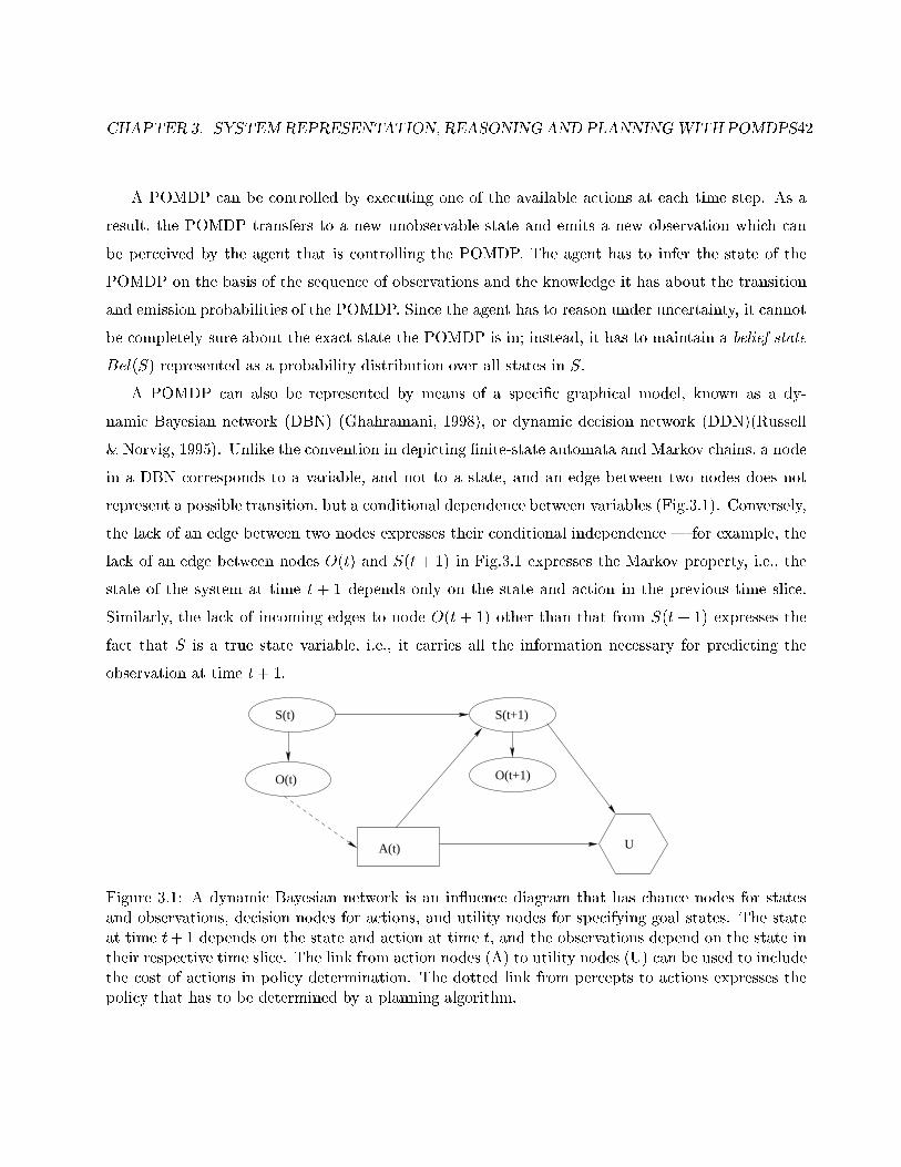
CHAPTER 3. SYSTEMREPRESENTATION, REASONING AND PLANNINGWITH POMDPS42
A POMDP can be controlled by executing one of the available actions at each time step. As a
result, the POMDP transfers to a new unobservable state and emits a new observation which can
be perceived by the agent that is controlling the POMDP. The agent has to infer the state of the
POMDP on the basis of the sequence of observations and the knowledge it has about the transition
and emission probabilities of the POMDP. Since the agent has to reason under uncertainty, it cannot
be completely sure about the exact state the POMDP is in; instead, it has to maintain a belief state
Bel(S) represented as a probability distribution over all states in S.
A POMDP can also be represented by means of a speci�c graphical model, known as a dy-
namic Bayesian network (DBN) (Ghahramani, 1998), or dynamic decision network (DDN)(Russell
& Norvig, 1995). Unlike the convention in depicting �nite-state automata and Markov chains, a node
in a DBN corresponds to a variable, and not to a state, and an edge between two nodes does not
represent a possible transition, but a conditional dependence between variables (Fig.3.1). Conversely,
the lack of an edge between two nodes expresses their conditional independence | for example, the
lack of an edge between nodes O(t) and S(t+ 1) in Fig.3.1 expresses the Markov property, i.e., the
state of the system at time t + 1 depends only on the state and action in the previous time slice.
Similarly, the lack of incoming edges to node O(t + 1) other than that from S(t + 1) expresses the
fact that S is a true state variable, i.e., it carries all the information necessary for predicting the
observation at time t+ 1.
O(t+1)
S(t+1)
A(t)
O(t)
S(t)
U
Figure 3.1: A dynamic Bayesian network is an in uence diagram that has chance nodes for statesand observations, decision nodes for actions, and utility nodes for specifying goal states. The stateat time t+1 depends on the state and action at time t, and the observations depend on the state intheir respective time slice. The link from action nodes (A) to utility nodes (U) can be used to includethe cost of actions in policy determination. The dotted link from percepts to actions expresses thepolicy that has to be determined by a planning algorithm.
CHAPTER 3. SYSTEMREPRESENTATION, REASONING AND PLANNINGWITH POMDPS43
3.2 Reasoning by Means of Belief Updating
At all times, the agent maintains a belief distribution Bel(S) over all possible states it can be
in, and updates it according to the actions it takes and the percepts it observes. This process of
belief updating follows a two-stage prediction-estimation cycle (Russell & Norvig, 1995; Koenig &
Simmons, 1998). During prediction, the agent estimates how the belief state at time t will change if
a particular action at�1 is performed at time t � 1, based on the belief state before the action was
performed and general knowledge about how actions a�ect states:
Bel(st) =X
st�12S
P (stjst�1; at�1)Bel(st�1);
where Bel(st) is the estimated belief state at time t for all states s in S, Bel(st�1) is the belief state
at time t� 1, P (stjst�1; at�1) are transition probabilities of the POMDP, and the sum runs over all
states in S.
During the estimation phase, the newly observed percept ot is used to update the estimated belief
vector:
Bel(st) = �P (otjst)Bel(st);
where P (otjst) are the emission probabilities of the POMDP and � is a normalization coeÆcient.
The most likely state at each step is the one whose corresponding element of the belief vector is
largest.
Reasoning in factorial POMDPs (DBNs with several state nodes) follows the same principle, but
is exponential in the number of nodes (state components or features) in the network, which might
cause computational diÆculties. Stochastic methods for belief updating have been applied to reduce
the time and space complexity of reasoning in DBNs (Binder et al., 1997; Kanazawa et al., 1995).
3.3 Planning with POMDPs
Controlling a POMDP amounts to choosing the correct actions that will maximize the expected
cumulative reward received by the agent over the course of its operation. When this course is in�nite
in duration, the sum itself will be in�nite | one way to avoid this is to apply an exponential
CHAPTER 3. SYSTEMREPRESENTATION, REASONING AND PLANNINGWITH POMDPS44
discounting factor < 1 to each reward. Thus, the goal of the controller is to maximize the quantity
<1Xt=0
tRt >;
where Rt is the reward received at the t-th step of operation, and < � > denotes expectation.
Many algorithms for choosing proper actions in POMDPs have been studied (Cassandra et al., 1996),
some of which are reviewed below.
One approach to controlling a POMDP that leads to optimal control is to transform the POMDP
into a fully observable MDP, whose states are the belief states of the original POMDP. Since the
space of all belief states is continuous and most methods for solving MDPs operate on discrete state,
the belief state is usually discretized. However, applying this method directly is extremely demanding
computationally and ineÆcient. In general, the problem of �nding optimal policies for POMDPs has
been proven to be PSPACE hard (Littman et al., 1995) and direct discretization of belief space can
only be used for trivial POMDPS with less than ten states.
More eÆcient algorithms exist as well, starting with the work of Sondik (Sondik, 1971), sub-
sequently improved by Kaelbling and Littman (Kaelbling et al., 1996). These improvements use
piece-wise-linear functions to represent the dependency of cumulative rewards on belief state. Even
though these algorithms o�er dramatic improvements in computational eÆciency, they are still ap-
plicable only to POMDPs with several tens of states. Because of the computational diÆculty of
�nding optimal solutions to POMDPs, various heuristic suboptimal strategies have been explored,
among which are assumptive planning and MDP-based approaches.
Assumptive planning
This heuristic strategy, proposed by Nourbakhsh (1998), performs full belief updating of its belief
state based on the transition and emission probabilities, as described in the previous sections, but
makes several simplifying assumptions when choosing an action. First, it assumes that it is in
the most likely state with complete certainty, thus ignoring the possibility of being in other states.
Next, it constructs a deterministic FSA from the transition and emission probabilities of the original
POMDP and uses a general search algorithm such as iterative deepening to �nd a path in the FSA.
Furthermore, the planner produces a list of percepts that ought to be seen if the plan is executed
and the FSA is a true representation of the world. However, in some cases the percepts seen by the
agent will di�er from the expected ones, which is an indication that the plan is no longer valid and
CHAPTER 3. SYSTEMREPRESENTATION, REASONING AND PLANNINGWITH POMDPS45
the agent is lost. If this is the case, the planner is invoked again to �nd a new plan based on the
latest estimate of the most likely state.
MDP-based strategies
Another set of heuristic strategies solves �rst the underlying MDP in hidden state variables (ignoring
the emission distribution E) and then makes use of that solution in conjunction with the estimated
belief state (Cassandra et al., 1996; Koenig & Simmons, 1998). This corresponds to the usual
approach taken in control engineering, where the problems of state estimation and control are solved
separately | a closed-loop control law is designed under the assumption that the state is completely
observable, and a separate observer is designed to estimate the current state.
The solution of the underlying MDP is an optimal policy that maps each state into the action that
maximizes the expected future cumulative reward. In order to �nd that action, an auxiliary function
Q(s; a) is computed, whose meaning is the expected cumulative reward if action a is performed in
state s and an optimal policy is followed thereafter. If the Q-function is known for a state, the
optimal action a� for that state is the one with highest Q-value: a�(s) = argmaxaQ(s; a). The
Q-function can also be de�ned recursively, describing the conditions that must be satis�ed for each
state-action pair in the MDP:
Q(s; a) =< R(s) + Xs02S
P (s0js; a)[maxb
Q(s0; b)] >;
where P (s0js; a) is the transition probability that the system will end up in state s0 if action
a is performed in state s. The resulting system of nonlinear equations for each state-action pair
can be solved by means of iterative relaxation techniques such as Jacobi and Gauss-Seidel iterations
(Bertsekas & Tsitsiklis, 1989), which are also known as Bellman back-ups in this case:
Qt+1(s; a) :=< R(s) + Xs02S
P (s0js; a)[maxb
Qt(s0; b)] > :
As a result of these iterations, the estimates Qt converge to the true Q function. It is also
possible to use Monte-Carlo methods such as Q-learning (Sutton & Barto, 1998). Instead of taking
expectations directly by forming sums, Q-learning samples transitions (s; a; s0; R) from the MDP
model or directly from the real world, and updates the estimates Qt according to:
CHAPTER 3. SYSTEMREPRESENTATION, REASONING AND PLANNINGWITH POMDPS46
Qt+1(s; a) := (1� �)Qt(s; a) + �[R(s) + maxb
Qt(s0; b)];
where Qt(s; a) is an estimate of the Q-function at iteration t, � is a learning rate coeÆcient, which
should decrease with time, and the state s0 is sampled according to the transition probabilities for
state s and action a (Jaakkola et al., 1994). Once the MDP is solved, the Q-values can be used in
several ways to approximate the optimal policy for the POMDP case (Cassandra et al., 1996; Koenig
& Simmons, 1998):
Most-likely-state method: The most likely state is found, as described in the previous subsection,
and the optimal action for that state is chosen. This method may be suboptimal if there is still
non-zero probability that the system is not in the most likely state and the optimal actions for
the ignored states are di�erent.
Voting method: This method chooses the action with highest probability mass in the belief vector.
For each action, the belief probabilities for the states where this action is optimal are added
up, and the action with the highest sum is chosen.
QMDP method: Similar to the voting method, but instead of adding up state beliefs only to the
sum of the winning action, they are added to the sums of all actions, weighted proportionally
to the actual Q-values. This avoids choosing the wrong action in cases when one action wins
by a small margin in several states, but loses badly in another state. The QMDP method would
be optimal if all uncertainty in the world was to suddenly disappear at the next time step.
All of the above methods based on the solution of the underlying MDP cannot plan to perform
an action solely to gain more information. Various strategies have been researched that aim to
reduce the degree of uncertainty as measured by the entropy of the belief vector (Cassandra et al.,
1996). Another approach, the SPOVA-RL algorithm due to Parr and Russell, uses a special-purpose
function approximator to estimate and represent the expected reward of each state following the
optimal policy for the POMDP (Parr & Russell, 1995). It has been reported to solve successfully
POMDPs with hundreds of states and actions.
In summary, if a POMDP model has a reasonably small number of states (up to a few thousand),
exact reasoning by belief propagation can be implemented very conveniently in real time. Planning

CHAPTER 3. SYSTEMREPRESENTATION, REASONING AND PLANNINGWITH POMDPS47
with POMDP models, on the other hand, can almost never be performed exactly, but approximate
planning algorithms are known and can be used eÆciently. The fact that such planning cannot be
performed in real time is not a problem, since once a policy is obtained, it is equivalent to a universal
plan and consulting such a policy when making control decisions is very fast. Overall, satisfactory
and eÆcient solutions exist for both reasoning and planning with POMDP models, if such models
are available to the robot. Learning such models is the main objective of this thesis and various
methods for doing this are explored in the next four chapters.
Chapter 4
Learning POMDP Models by Iterative
Adjustment of Probabilities
Since a POMDP model is just a particular type of a probabilistic model, the most obvious approach
to learning such models is to apply general algorithms for learning probabilistic networks from data,
such as those proposed in (Heckerman et al., 1995; Russell et al., 1994). Assuming that the structure
of the POMDP model is known, the goal of learning is to �nd appropriate values for the entries in
the transition and emission local conditional probability tables (LCPTs) of a POMDP model which
maximize the log-likelihood lnP (Djw) that the training data set D was generated by the POMDP
with parameters w. Each case Dl from the data set D consists of assignments for the observable
nodes in O.
Two algorithms for learning probabilistic networks can readily be adapted to the problem of
learning POMDPs: the algorithm proposed by Russell et al. (1994), and the Baum-Welch algorithm,
widely used for learning Hidden Markov Models (HMMs) (Rabiner & Juang, 1986). These two
algorithms and their application to POMDP learning are described below and investigated for the
problem of recovering the probabilities of a POMDP with the explicit purpose to use this model for
planning.
48
CHAPTER 4. LEARNING POMDPMODELS BY ITERATIVE ADJUSTMENTOF PROBABILITIES49
4.1 Steepest Gradient Ascent (SGA) in Likelihood
Russell et al. (1994) proposed a particularly simple learning rule which performs steepest gradient
ascent in the space of LCPT entries wijk:
�wijk = �NXt=1
@P (Dtjw)=@wijk
P (Dtjw)=
NXt=1
P (xij ;uikjDt;w)
wijk
;
wijk = P (xijjuik) = P (Xi = xij jUi = uik)
where wijk is the entry of the LCPT of variable node Xi that designates the probability that
this node Xi will be in its j-th state xij given that its parents Ui are in their k-th con�guration uik
(Russell et al., 1994). The parameters wijk can be either those parametrizing the transition function
T , or the emission function E, depending on which nodes the learning rule is applied to. Referring
to Fig. 3.1, for a POMDP model with one state and one observation variable, the node Xi can either
be the observation O, in which case xij = oj, or the state node S, in which case xij = sj. The parent
sets Ui and their con�gurations are also evident in Fig. 3.1. The speed of ascent along the gradient
is controlled by the rate parameter �.
The summation index t = 1; N runs over all data cases Dt in D. (In case there are more
than one observation variables, the observations Dt at time t form a vector, and we will denote
its i-th component in the observation trace as Dt;i.) As pointed out in (Russell et al., 1994), the
quantity P (xij ;uikjDt;w) can be obtained by means of belief updating in a general-purpose belief
net reasoning system. Furthermore, since the transition and emission probabilities are the same for
all time slices, the estimates for the same probability in all time slices are averaged.
4.2 Baum-Welch
Chrisman (1992) and Koenig and Simmons (1998) adapted the Baum-Welch (BW) algorithm for
learning HMMs to the problem of improving the entries of the LCPTs of POMDP models from data.
BW is a variant of the EM algorithm popular in statistics. The learning rule of the Baum-Welch
algorithm for the transition probabilities of an HMM is:
CHAPTER 4. LEARNING POMDPMODELS BY ITERATIVE ADJUSTMENTOF PROBABILITIES50
wm+1ijk =
PNt=1 �
mi;t(j; k)PN
t=1 mi;t(j)
;
where wm+1ijk is the estimate of the transition probability P [Si = xij jUi = uik] that node Si will
be in its j-th state sij given that its parents Ui are in their k-th con�guration uik, after iteration
m+ 1, and
�mi;t(j; k) = P [Si(t+ 1) = sik;Ui(t) = uikjD; wm]
mi;t(j) = P [Ui(t) = uij jD; wm]:
Here D refers to the whole sequence, t ranges over all observations in D, and m is the iteration
number of the Baum-Welch algorithm. For an HMM with a single state node, i = 1. It can be seen
that the quantity �i;t(j; k) is in fact used in Steepest Gradient Ascent (SGA) too. For a DBN, the
learning rule of SGA for its transition probabilities can also be written as:
wm+1ijk = wm
ijk + �
PNt=1 �
mi;t(j; k)
wmijk
That is, Baum-Welch and the Steepest Gradient Ascent algorithm make use of the same quan-
tities, but in quite a di�erent manner: while the SGA algorithm performs small steps in parameter
space around the previous estimate of the parameter, Baum-Welch completely re-estimates the pa-
rameter value.
Unlike the SGA algorithm, Baum-Welch uses di�erent reestimation formulae for transition and
emission probabilities. If the parameter wijk represents the emission probability that observable
variable Oi (i-th component of the observation vector D) has its j-th discrete value given that its
parents (state nodes) are in their k-th con�guration, its reestimation formula is
wm+1ijk =
PNt=1;s:t:Dt;i=j
mt (k)PNt=1
mt (k)
;
where the sum in the numerator includes only the state probabilities mt (k) for moments t when
the i-th component Dt;i of the vector Dt in the training sequence had assumed the j-th value of
output variable Oi. As above, if there is only one observation variable, i = 1. The quantity mt (k) is
CHAPTER 4. LEARNING POMDPMODELS BY ITERATIVE ADJUSTMENTOF PROBABILITIES51
the probability that the state (hidden) variables that are parents of the observation variables are in
their k-th con�guration at time t.
4.3 Experimental Comparison between BW and SGA
Since both BW and SGA are well-known and established algorithms, the very �rst experiment was to
verify how they work on the simplest possible probabilistic models: an HMM with two states s1 and
s2 and two discrete observations o1 and o2, and a POMDP model with the same number of states
and observations, but also with two actions a1 and a2. The objective of this experiment was to �nd
out whether these two algorithms could recover completely the transition probabilities of the HMM
and the POMDP model. Note that this objective is di�erent from the usual objective of training
HMMs for the purposes of speech recognition, for example; while in speech recognition an HMM is
used for classi�cation and it is not important what values of its parameters would achieve a high
accuracy rate, our goal is to use the actual recovered probabilities with approximate DTP planning
algorithms.
SGA and BW were �rst tested on the HMM, providing the algorithms with a training data set
with 500 data cases generated by logical sampling of the known HMM, i.e., these cases were drawn
from the probabilistic distribution represented by the HMM. The process of logical sampling consists
of generating random assignments for child nodes according to the LCPTs for these nodes and the
assignments for their parent nodes. The process starts with the base nodes, which have no parents,
and proceeds according to the principal ordering of the nodes in the HMM. The learning algorithm
is only allowed to see the values of the observable nodes.
In these experiments, the HMM to be learned was initialized with the correct emission distribu-
tion. The objective of learning was to �nd the transition probabilities P [S(t+ 1)jS(t)].
A number of trial runs were performed, with di�erent emission and transition distributions,
varying the amount of uncertainty in them. It was found that, in general, Baum-Welch was much
more successful than SGA in learning the parameters of this particular HMM. For illustration, the
increase in log-likelihood of the data for the two algorithms is plotted against the iteration number
in Fig. 4.1. Since the computational complexity of a single step of BW and SGA is comparable |
in both cases, it is linear in the number of hidden states N | the graph also demonstrates how fast
each algorithm converges to the closest local maximum in likelihood.
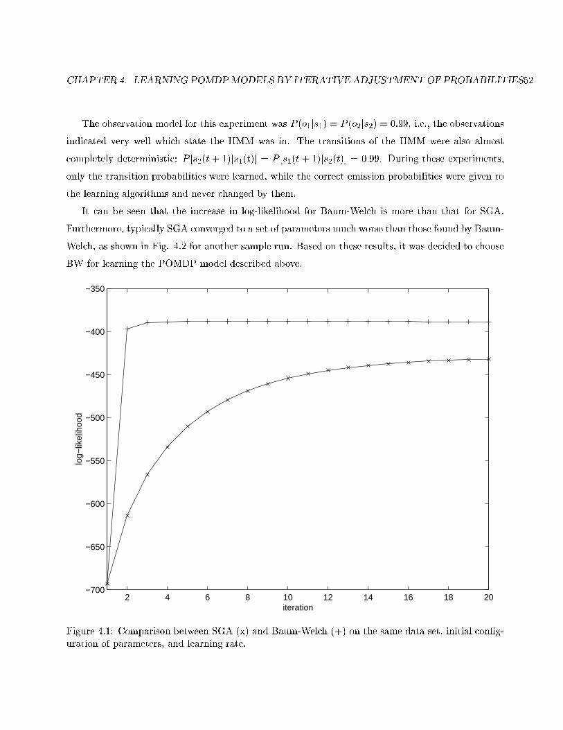
CHAPTER 4. LEARNING POMDPMODELS BY ITERATIVE ADJUSTMENTOF PROBABILITIES52
The observation model for this experiment was P (o1js1) = P (o2js2) = 0:99, i.e., the observations
indicated very well which state the HMM was in. The transitions of the HMM were also almost
completely deterministic: P [s2(t + 1)js1(t)] = P [s1(t + 1)js2(t)] = 0:99. During these experiments,
only the transition probabilities were learned, while the correct emission probabilities were given to
the learning algorithms and never changed by them.
It can be seen that the increase in log-likelihood for Baum-Welch is more than that for SGA.
Furthermore, typically SGA converged to a set of parameters much worse than those found by Baum-
Welch, as shown in Fig. 4.2 for another sample run. Based on these results, it was decided to choose
BW for learning the POMDP model described above.
2 4 6 8 10 12 14 16 18 20−700
−650
−600
−550
−500
−450
−400
−350
iteration
log−
likel
ihoo
d
Figure 4.1: Comparison between SGA (x) and Baum-Welch (+) on the same data set, initial con�g-uration of parameters, and learning rate.
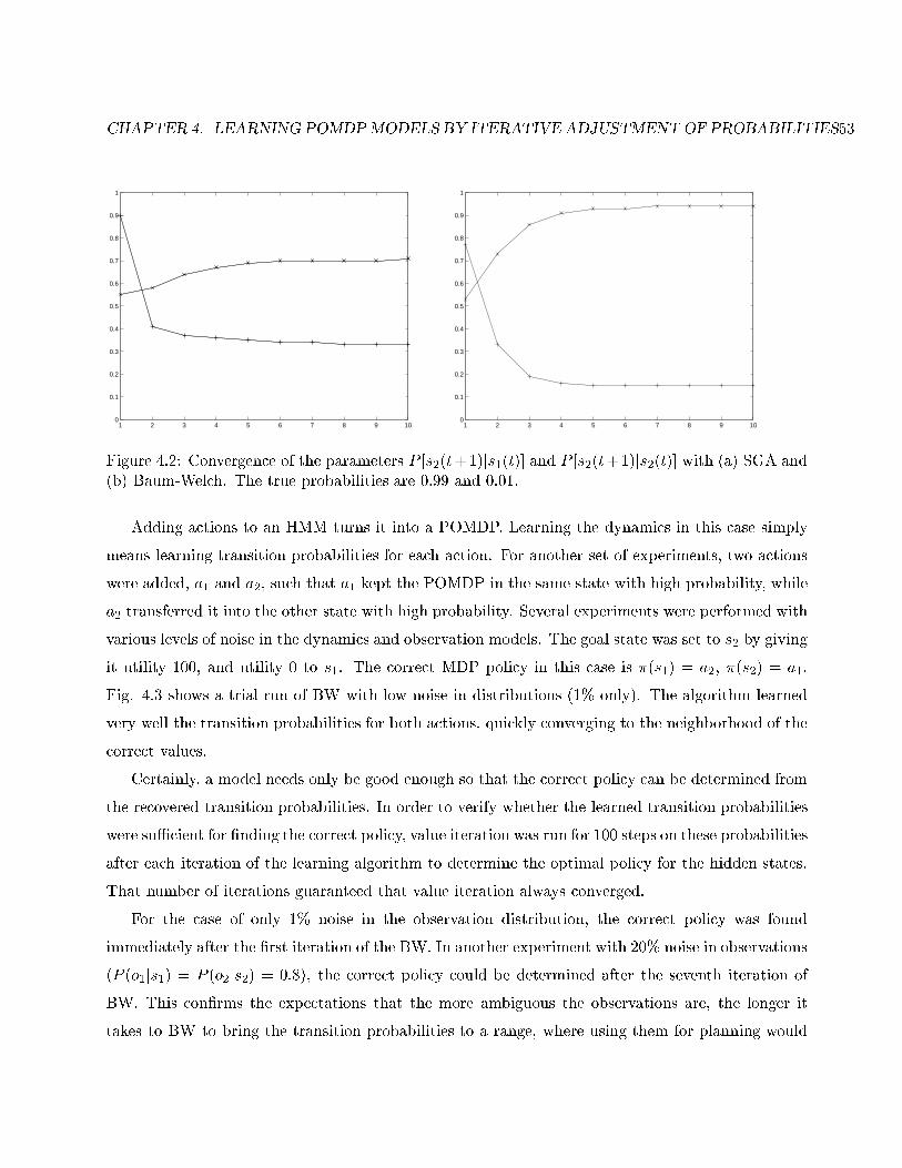
CHAPTER 4. LEARNING POMDPMODELS BY ITERATIVE ADJUSTMENTOF PROBABILITIES53
1 2 3 4 5 6 7 8 9 100
0.1
0.2
0.3
0.4
0.5
0.6
0.7
0.8
0.9
1
1 2 3 4 5 6 7 8 9 100
0.1
0.2
0.3
0.4
0.5
0.6
0.7
0.8
0.9
1
Figure 4.2: Convergence of the parameters P [s2(t+1)js1(t)] and P [s2(t+1)js2(t)] with (a) SGA and(b) Baum-Welch. The true probabilities are 0:99 and 0:01.
Adding actions to an HMM turns it into a POMDP. Learning the dynamics in this case simply
means learning transition probabilities for each action. For another set of experiments, two actions
were added, a1 and a2, such that a1 kept the POMDP in the same state with high probability, while
a2 transferred it into the other state with high probability. Several experiments were performed with
various levels of noise in the dynamics and observation models. The goal state was set to s2 by giving
it utility 100, and utility 0 to s1. The correct MDP policy in this case is �(s1) = a2, �(s2) = a1.
Fig. 4.3 shows a trial run of BW with low noise in distributions (1% only). The algorithm learned
very well the transition probabilities for both actions, quickly converging to the neighborhood of the
correct values.
Certainly, a model needs only be good enough so that the correct policy can be determined from
the recovered transition probabilities. In order to verify whether the learned transition probabilities
were suÆcient for �nding the correct policy, value iteration was run for 100 steps on these probabilities
after each iteration of the learning algorithm to determine the optimal policy for the hidden states.
That number of iterations guaranteed that value iteration always converged.
For the case of only 1% noise in the observation distribution, the correct policy was found
immediately after the �rst iteration of the BW. In another experiment with 20% noise in observations
(P (o1js1) = P (o2js2) = 0:8), the correct policy could be determined after the seventh iteration of
BW. This con�rms the expectations that the more ambiguous the observations are, the longer it
takes to BW to bring the transition probabilities to a range, where using them for planning would
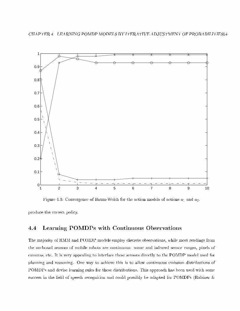
CHAPTER 4. LEARNING POMDPMODELS BY ITERATIVE ADJUSTMENTOF PROBABILITIES54
1 2 3 4 5 6 7 8 9 100
0.1
0.2
0.3
0.4
0.5
0.6
0.7
0.8
0.9
1
Figure 4.3: Convergence of Baum-Welch for the action models of actions a1 and a2.
produce the correct policy.
4.4 Learning POMDPs with Continuous Observations
The majority of HMM and POMDP models employ discrete observations, while most readings from
the on-board sensors of mobile robots are continuous: sonar and infrared sensor ranges, pixels of
cameras, etc. It is very appealing to interface these sensors directly to the POMDP model used for
planning and reasoning. One way to achieve this is to allow continuous emission distributions of
POMDPs and devise learning rules for these distributions. This approach has been used with some
success in the �eld of speech recognition and could possibly be adapted for POMDPs (Rabiner &
CHAPTER 4. LEARNING POMDPMODELS BY ITERATIVE ADJUSTMENTOF PROBABILITIES55
Juang, 1986).
In order to verify whether this was possible, several experiments were performed on hybrid
POMDPs with discrete state variables and continuous observations. Fig. 4.4 demonstrates the
results of learning a two-state POMDP with three continuous observable variables, one of which is
the reinforcement from the environment and the other two are indicative of the state of the POMDP,
although they do not determine it unambiguously. A total of 50 cases were generated from a known
POMDP. The observation models were unimodal Gaussian distributions with variance one and means
(10; 5) and (5; 10) for the two states, respectively. Reward was 0 for state one and 1 for state two.
Analogously to the previous section, two actions were de�ned: for each of the two states, the �rst
action a1 kept the POMDP in the same state, while the second action a2 moved it to the other state.
Each of the actions succeeded with probability 0:9.
The learned model also had Gaussian emission distributions, with �xed variance equal to that
of the true model. This signi�cantly constrains learning and helps the learning algorithm. The
objective of the algorithm is reduced to only �nding the correct means of the Gaussian distributions.
Fig. 4.4a shows the process of grounding the two states in the space of continuous observations. Fig.
4.4b demonstrates how the transition distribution of the POMDP is being learned simultaneously
with the grounding of the states. Fig. 4.4c traces the convergence of the log-likelihood of the learned
model to that of the true model, which was used to generate the data cases.
After ten iterations of the learning algorithm for the POMDP model, the learned state transition
matrix was used together with the learned utility to determine the optimal action in each state. Value
iteration with discounting factor of 0:7 was performed over 20 iterations. The resulting Q-values for
each state are plotted in Fig. 4.4d. It can be seen that the learned policy is correct, even though
the learned state transition probabilities are quite far from their true values. This happens in spite
of the fact that the likelihood of the learned model converges to that of the true model, as seen in
Fig. 4.4a, and BW is apparently not stuck in a local maximum of likelihood.
These results are indicative of what can be expected from the Baum-Welch algorithm. Recovering
completely the transition probabilities of the POMDP is very hard even in cases when the algorithm
does not reach a local maximum in likelihood, but almost reaches the likelihood of the true model.
This indicates a serious problem for the application of BW to recovering transition probabilities: it
is very hard for BW to drive them into close proximity to their true values, because the gradient
of the likelihood with respect to these probabilities is very small around the true global maximum
CHAPTER 4. LEARNING POMDPMODELS BY ITERATIVE ADJUSTMENTOF PROBABILITIES56
of likelihood. This fact, although discovered a long time ago (Rabiner et al., 1985), is not widely
known, because it does not a�ect signi�cantly the major practical application of learned probabilistic
models | speech recognition. There are two reasons for this. The �rst is the way HMMs are used
in speech recognition | several learned HMM models are matched against a novel voice sequence,
and classi�ed to the class of the model that has the highest likelihood for this sequence. Exactly
what probabilities are used in this classi�cation process is not important. The second reason is the
lack of any ground truth to compare the learned model with | the training data are produced by
a vocal tract, and not by an actual probabilistic model. This is in contrast to the problem we are
considering, where a model can often be created manually, for example from a geometric map of the
environment as in (Koenig & Simmons, 1998), and discrepancies between it and a learned model can
easily be noticed.
Furthermore, experience suggests that local maxima are very common during the process of
learning the POMDP model. This is also a well-known fact that results from the nature of continuous
system representations with POMDP models (Rabiner et al., 1985; Rabiner & Juang, 1986). A
suggested remedy for this problem has been to perform initially k-means clustering, and provide the
centers of the clusters as initial estimates for the means of the observation models (Rabiner et al.,
1985).
4.4.1 Clustering of Observations
In order to verify this clustring solution, infrared sensor data were collected from a Nomad 150 sim-
ulator provided by Nomadic Technologies Inc., Mountain View, California (Nomadic-Technologies,
1997) in another set of experiments. The Nomad 150 robot is equipped with 16 infrared sensors,
which give proximity readings in the range of 0� 36 inches. The readings have relatively low noise
and high repeatability, but because of their limited range, the robot often experiences signi�cant
perceptual aliasing.
A robot was placed in the world shown in Fig. 4.5, where three actions were available: moving
forward 25 inches, turning left 90 degrees and turning right 90 degrees. If the robot could not
complete a move forward, it returned back to its original position.
Because of the size of the world and the available actions, the robot could be at only one of seven
locations and four orientations. However, because the simulator supports slippage, these locations
and orientations vary slightly during the course of movement of the robot. Furthermore, this drift
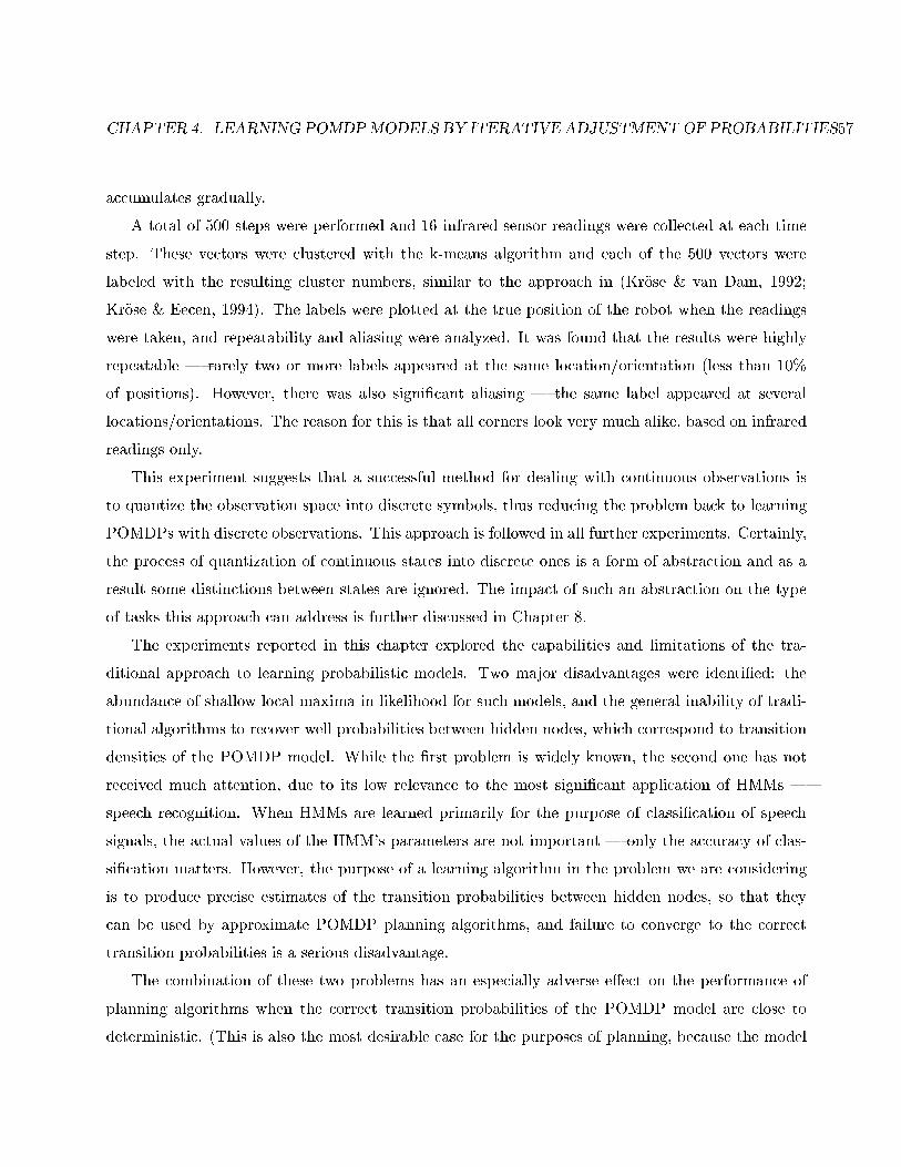
CHAPTER 4. LEARNING POMDPMODELS BY ITERATIVE ADJUSTMENTOF PROBABILITIES57
accumulates gradually.
A total of 500 steps were performed and 16 infrared sensor readings were collected at each time
step. These vectors were clustered with the k-means algorithm and each of the 500 vectors were
labeled with the resulting cluster numbers, similar to the approach in (Kr�ose & van Dam, 1992;
Kr�ose & Eecen, 1994). The labels were plotted at the true position of the robot when the readings
were taken, and repeatability and aliasing were analyzed. It was found that the results were highly
repeatable | rarely two or more labels appeared at the same location/orientation (less than 10%
of positions). However, there was also signi�cant aliasing | the same label appeared at several
locations/orientations. The reason for this is that all corners look very much alike, based on infrared
readings only.
This experiment suggests that a successful method for dealing with continuous observations is
to quantize the observation space into discrete symbols, thus reducing the problem back to learning
POMDPs with discrete observations. This approach is followed in all further experiments. Certainly,
the process of quantization of continuous states into discrete ones is a form of abstraction and as a
result some distinctions between states are ignored. The impact of such an abstraction on the type
of tasks this approach can address is further discussed in Chapter 8.
The experiments reported in this chapter explored the capabilities and limitations of the tra-
ditional approach to learning probabilistic models. Two major disadvantages were identi�ed: the
abundance of shallow local maxima in likelihood for such models, and the general inability of tradi-
tional algorithms to recover well probabilities between hidden nodes, which correspond to transition
densities of the POMDP model. While the �rst problem is widely known, the second one has not
received much attention, due to its low relevance to the most signi�cant application of HMMs |
speech recognition. When HMMs are learned primarily for the purpose of classi�cation of speech
signals, the actual values of the HMM's parameters are not important | only the accuracy of clas-
si�cation matters. However, the purpose of a learning algorithm in the problem we are considering
is to produce precise estimates of the transition probabilities between hidden nodes, so that they
can be used by approximate POMDP planning algorithms, and failure to converge to the correct
transition probabilities is a serious disadvantage.
The combination of these two problems has an especially adverse e�ect on the performance of
planning algorithms when the correct transition probabilities of the POMDP model are close to
deterministic. (This is also the most desirable case for the purposes of planning, because the model

CHAPTER 4. LEARNING POMDPMODELS BY ITERATIVE ADJUSTMENTOF PROBABILITIES58
is less ambiguous.) If learning starts with random initial values, which in general correspond to
high entropy in transition distributions, the trajectory that has to be followed in parameter space
by the learning algorithm to get to deterministic (low-entropy) regions would be very long, and the
risk of converging to a shallow local maximum in likelihood would increase. Furthermore, failing to
converge to the correct (nearly) deterministic transition distributions can impact negatively heuristic
methods such as assumptive planning, which simplify the POMDP into an FSA and would perform
best if the loss of precision due to the simpli�cation is minimal.
It is clear that this behavior of the traditional learning methods presents a severe disadvantage,
and alternative approaches have to be explored.
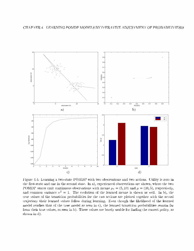
CHAPTER 4. LEARNING POMDPMODELS BY ITERATIVE ADJUSTMENTOF PROBABILITIES59
0 5 10 150
5
10
15
observation O1
obse
rvat
ion
O2
0 0.1 0.2 0.3 0.4 0.5 0.6 0.7 0.8 0.9 10
0.1
0.2
0.3
0.4
0.5
0.6
0.7
0.8
0.9
1
P(S1|S1)
P(S
2|S
2)
a) b)
0 1 2 3 4 5 6 7 8 9 10
−160
−140
−120
−100
−80
−60
−40
−20
0
iteration
log−
likel
ihoo
d
1 20
0.5
1
1.5
2
2.5
state
Q(s
,a)
a1a2
c) d)
Figure 4.4: Learning a two-state POMDP with two observations and two actions. Utility is zero inthe �rst state and one in the second state. In a), experienced observations are shown, where the twoPOMDP states emit continuous observations with means �1 = (5; 10) and � = (10; 5), respectively,and common variance �2 = 1. The evolution of the learned means is shown as well. In b), thetrue values of the transition probabilities for the two actions are plotted together with the actualtrajectory their learned values follow during learning. Even though the likelihood of the learnedmodel reaches that of the true model as seen in c), the learned transition probabilities remain farfrom their true values, as seen in b). These values are barely usable for �nding the correct policy, asshown in d).
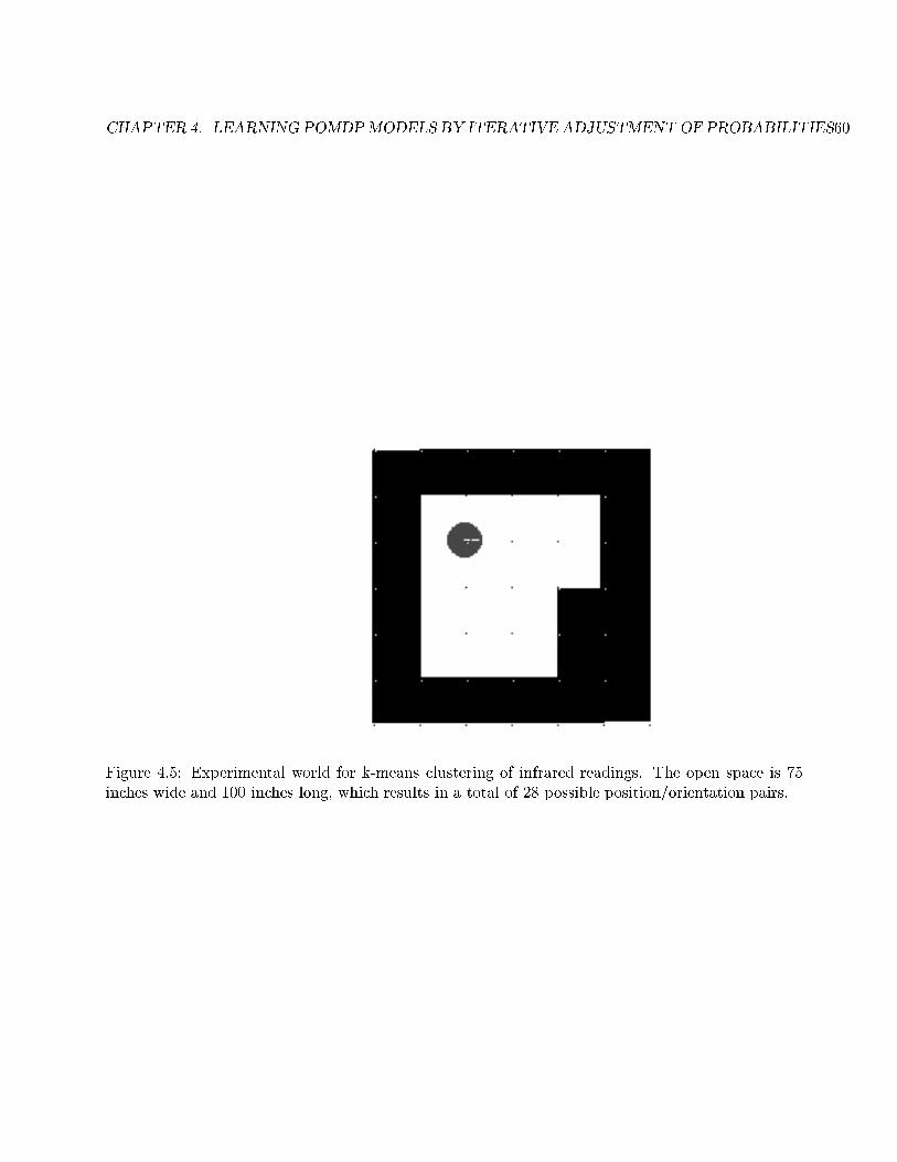
CHAPTER 4. LEARNING POMDPMODELS BY ITERATIVE ADJUSTMENTOF PROBABILITIES60
Figure 4.5: Experimental world for k-means clustering of infrared readings. The open space is 75inches wide and 100 inches long, which results in a total of 28 possible position/orientation pairs.
Chapter 5
Learning POMDP Models by State
Aggregation
The previous chapter identi�ed two major disadvantages of learning algorithms such as Baum-Welch
and Steepest Gradient Ascent (SGA) when applied to recovering transition probabilities in models
with hidden state. In this chapter, a radically di�erent approach to learning models with hidden
state is explored | that of aggregating states into equivalence classes. This method has been
explored in the �eld of operations research for the problem of solving completely speci�ed MDPs
with very large state spaces (Chatelin & Miranker, 1982; Bertsekas & Casta~non, 1989). The second
algorithm proposed in this section (SMTC) also bears close similarity to the dominant methods
in system identi�cation as performed in the �eld of control engineering, although its algorithmic
implementation di�ers signi�cantly from these methods.
5.1 Best-First Model Merging
A completely di�erent method for learning HMMs has been suggested by Stolcke and Omohundro,
originally for the purposes of speech recognition (Stolcke & Omohundro, 1993). Their approach
consists of building an initial HMM, which has a separate state st for each time step in the observation
sequence. The transition and emission tables of this HMM are trivial { state st transitions to state
st+1 with probability one, and emits observation ot with probability one. Clearly, this HMM explains
the observation sequence perfectly, but is not the most compact model that can be learned from the
61
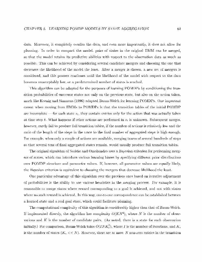
CHAPTER 5. LEARNING POMDP MODELS BY STATE AGGREGATION 62
data. Moreover, it completely over�ts the data, and even more importantly, it does not allow for
planning. In order to compact the model, pairs of states in the original HMM can be merged,
so that the model retains its predictive abilities with respect to the observation data as much as
possible. This can be achieved by considering several candidate mergers and choosing the one that
decreases the likelihood of the model the least. After a merger is chosen, a new set of mergers is
considered, and this process continues until the likelihood of the model with respect to the data
becomes unacceptably low, or a predetermined number of states is reached.
This algorithm can be adapted for the purposes of learning POMDPs by conditioning the tran-
sition probabilities of successor states not only on the previous state, but also on the action taken,
much like Koenig and Simmons (1996) adapted Baum-Welch for learning POMDPs. One important
caveat when moving from HMMs to POMDPs is that the transition tables of the initial POMDP
are incomplete | for each state st, they contain entries only for the action that was actually taken
at time step t. What happens if other actions are performed in st is unknown. Subsequent merges,
however, rarely fail to produce full transition tables, if the number of actions is relatively low and the
ratio of the length of the steps in the trace to the �nal number of aggregated steps is high enough.
For example, when only a couple of actions are available, merging traces of several hundreds of steps
so that several tens of �nal aggregated states remain, would usually produce full transition tables.
The original algorithm of Stolcke and Omohundro uses a Bayesian criterion for performing merg-
ers of states, which can introduce various learning biases by specifying di�erent prior distributions
over POMDP structure and parameter values. If, however, all parameter values are equally likely,
the Bayesian criterion is equivalent to choosing the mergers that decrease likelihood the least.
One particular advantage of this algorithm over the previous ones based on iterative adjustment
of probabilities is the ability to use various heuristics in the merging process. For example, it is
reasonable to merge states where reward corresponding to a goal is achieved, and not with states
where no such reward is achieved. In this way, one-to-one correspondence can be established between
a learned state and a real goal state, which could facilitate planning.
The computational complexity of this algorithm is considerably higher than that of Baum-Welch.
If implemented directly, the algorithm has complexity O(KN4), where N is the number of obser-
vations and K is the number of candidate pairs. (As noted, there is a state for each observation
initially.) For comparison, Baum-Welch takes O(INK2s ), where I is the number of iterations, and Ks
is the number of states (Ks << N). However, there are at most N non-zero entries in the transition
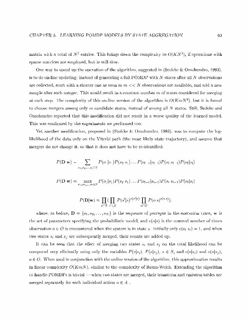
CHAPTER 5. LEARNING POMDP MODELS BY STATE AGGREGATION 63
matrix with a total of N2 entries. This brings down the complexity to O(KN3), if operations with
sparse matrices are employed, but is still slow.
One way to speed up the operation of the algorithm, suggested in (Stolcke & Omohundro, 1993),
is to do on-line updating: instead of generating a full POMDP with N states after all N observations
are collected, start with a shorter one as soon as m << N observations are available, and add a new
sample after each merger. This would result in a constant numberm of states considered for merging
at each step. The complexity of this on-line version of the algorithm is O(KmN2), but it is forced
to choose mergers among only m candidate states, instead of among all N states. Still, Stolcke and
Omohundro reported that this modi�cation did not result in a worse quality of the learned model.
This was con�rmed by the experiments we performed too.
Yet another modi�cation, proposed in (Stolcke & Omohundro, 1993), was to compute the log-
likelihood of the data only on the Viterbi path (the most likely state trajectory), and assume that
mergers do not change it, so that it does not have to be re-identi�ed:
P (Djw) =X
s1;s2;:::;sl2S
P (o1js1)P (s2js1) : : : P (ol�1jsl�1)P (sljsl�1)P (oljsl)
P (Djw) � maxs1;s2;:::;sl2S
P (o1js1)P (s2js1) : : : P (ol�1jsl�1)P (sljsl�1)P (oljsl)
P (Djw) �Ys2S
(Ys02S
P (s0js)c(s0js)
Yo2O
P (ojs)c(ojs));
where, as before, D = fo1; o2; : : : ; oNg is the sequence of percepts in the execution trace, w is
the set of parameters specifying the probabilistic model, and c(ojs) is the counted number of times
observation o 2 O is encountered when the system is in state s. Initially only c(oljsl) = 1, and when
two states si and sj are subsequently merged, their counts are added up.
It can be seen that the e�ect of merging two states si and sj on the total likelihood can be
computed very eÆciently using only the variables P (sjsi), P (sjsj), s 2 S, and c(ojsi) and c(ojsj),
o 2 O. When used in conjunction with the online version of the algorithm, this approximation results
in linear complexity O(KmN), similar to the complexity of Baum-Welch. Extending the algorithm
to handle POMDPs is trivial | when two states are merged, their transition and emission tables are
merged separately for each individual action a 2 A .
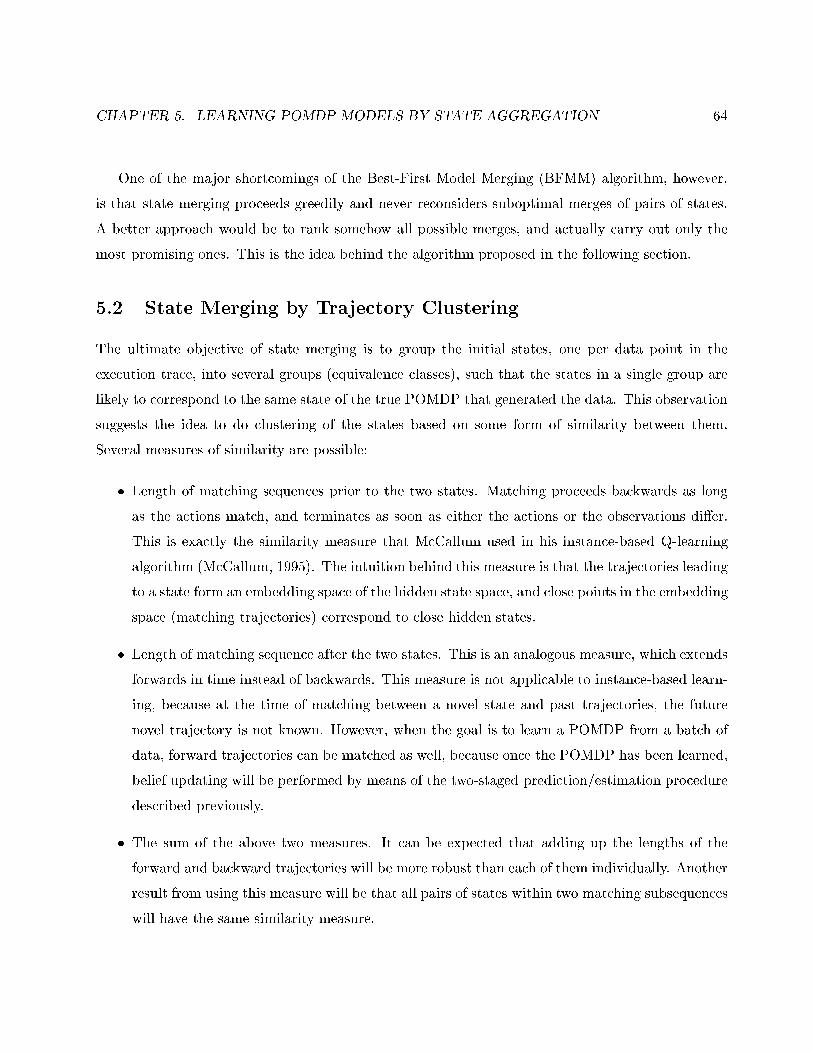
CHAPTER 5. LEARNING POMDP MODELS BY STATE AGGREGATION 64
One of the major shortcomings of the Best-First Model Merging (BFMM) algorithm, however,
is that state merging proceeds greedily and never reconsiders suboptimal merges of pairs of states.
A better approach would be to rank somehow all possible merges, and actually carry out only the
most promising ones. This is the idea behind the algorithm proposed in the following section.
5.2 State Merging by Trajectory Clustering
The ultimate objective of state merging is to group the initial states, one per data point in the
execution trace, into several groups (equivalence classes), such that the states in a single group are
likely to correspond to the same state of the true POMDP that generated the data. This observation
suggests the idea to do clustering of the states based on some form of similarity between them.
Several measures of similarity are possible:
� Length of matching sequences prior to the two states. Matching proceeds backwards as long
as the actions match, and terminates as soon as either the actions or the observations di�er.
This is exactly the similarity measure that McCallum used in his instance-based Q-learning
algorithm (McCallum, 1995). The intuition behind this measure is that the trajectories leading
to a state form an embedding space of the hidden state space, and close points in the embedding
space (matching trajectories) correspond to close hidden states.
� Length of matching sequence after the two states. This is an analogous measure, which extends
forwards in time instead of backwards. This measure is not applicable to instance-based learn-
ing, because at the time of matching between a novel state and past trajectories, the future
novel trajectory is not known. However, when the goal is to learn a POMDP from a batch of
data, forward trajectories can be matched as well, because once the POMDP has been learned,
belief updating will be performed by means of the two-staged prediction/estimation procedure
described previously.
� The sum of the above two measures. It can be expected that adding up the lengths of the
forward and backward trajectories will be more robust than each of them individually. Another
result from using this measure will be that all pairs of states within two matching subsequences
will have the same similarity measure.
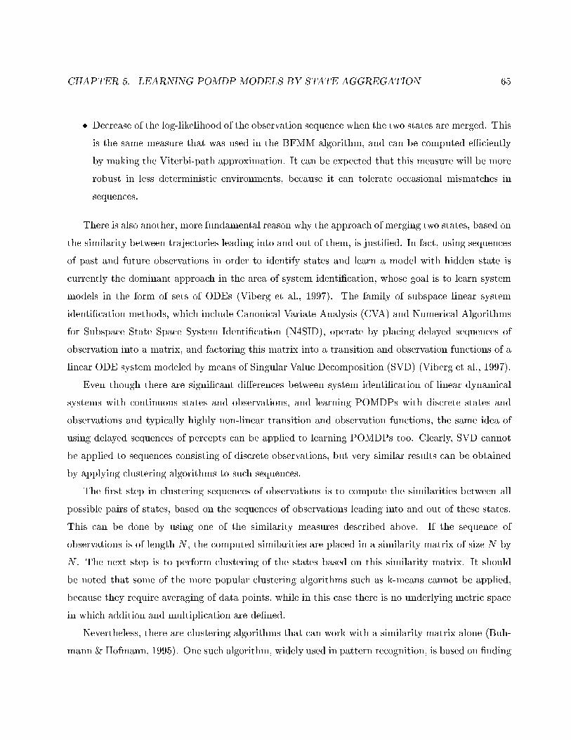
CHAPTER 5. LEARNING POMDP MODELS BY STATE AGGREGATION 65
� Decrease of the log-likelihood of the observation sequence when the two states are merged. This
is the same measure that was used in the BFMM algorithm, and can be computed eÆciently
by making the Viterbi-path approximation. It can be expected that this measure will be more
robust in less deterministic environments, because it can tolerate occasional mismatches in
sequences.
There is also another, more fundamental reason why the approach of merging two states, based on
the similarity between trajectories leading into and out of them, is justi�ed. In fact, using sequences
of past and future observations in order to identify states and learn a model with hidden state is
currently the dominant approach in the area of system identi�cation, whose goal is to learn system
models in the form of sets of ODEs (Viberg et al., 1997). The family of subspace linear system
identi�cation methods, which include Canonical Variate Analysis (CVA) and Numerical Algorithms
for Subspace State Space System Identi�cation (N4SID), operate by placing delayed sequences of
observation into a matrix, and factoring this matrix into a transition and observation functions of a
linear ODE system modeled by means of Singular Value Decomposition (SVD) (Viberg et al., 1997).
Even though there are signi�cant di�erences between system identi�cation of linear dynamical
systems with continuous states and observations, and learning POMDPs with discrete states and
observations and typically highly non-linear transition and observation functions, the same idea of
using delayed sequences of percepts can be applied to learning POMDPs too. Clearly, SVD cannot
be applied to sequences consisting of discrete observations, but very similar results can be obtained
by applying clustering algorithms to such sequences.
The �rst step in clustering sequences of observations is to compute the similarities between all
possible pairs of states, based on the sequences of observations leading into and out of these states.
This can be done by using one of the similarity measures described above. If the sequence of
observations is of length N , the computed similarities are placed in a similarity matrix of size N by
N . The next step is to perform clustering of the states based on this similarity matrix. It should
be noted that some of the more popular clustering algorithms such as k-means cannot be applied,
because they require averaging of data points, while in this case there is no underlying metric space
in which addition and multiplication are de�ned.
Nevertheless, there are clustering algorithms that can work with a similarity matrix alone (Buh-
mann & Hofmann, 1995). One such algorithm, widely used in pattern recognition, is based on �nding
CHAPTER 5. LEARNING POMDP MODELS BY STATE AGGREGATION 66
minimum spanning trees (MST) in the graph whose adjacency structure is de�ned by the similarity
matrix (Duda & Hart, 1973). Once the MST is found, the edges corresponding to the the least
similar pairings are severed. This results in several cliques, which de�ne clusters of states that are
likely to correspond to the same state in the true POMDP that generated the observations. The
last step of this algorithm for state merging by trajectory clustering (SMTC) is to assign consecutive
numbers to the remaining cliques, label the hidden states in the observation sequence with their
respective clique numbers, and estimate the transition and emission probabilities of the POMDP as
if it was fully observable.
This approach is likely to give better results than BFMM, because it considers all possible merges
before actually carrying out any of them. Furthermore, this method is guaranteed to recover com-
pletely a fully observable POMDP, while this is not necessarily true for EM and BFMM. Thus, it can
be expected that SMTC would outperform EM and BFMM in worlds, which are mildly unobservable,
such as environments with moderate perceptual aliasing.
Just like with BFMM, this algorithm is quite expensive computationally, if implemented directly.
Finding the similarity matrix from a sequence of N observations has a worst-case running time of
O(N3), because N2 matches are considered, and the length of the matching subsequences backwards
and forwards can be as long as N elements. In practice, though, most matches will terminate
after few time steps. Still, the complexity of �nding the MST given the similarity matrix of N2
elements is O(N3), if Prim's algorithm is used, and O(N2 logN), if Kruskal's algorithm is employed
in combination with a fast sorting routine (Cormen et al., 1991). Finally, the clique-labeling stage
takes computations in the order of N3, if matrix multiplications are used to determine adjacency
between members within a clique.
However, there are several algorithmic improvements that can bring the worst-case running time
down to O(N2) and the average running time to O(N logN). EÆcient subsequence matching al-
gorithms have been investigated in the �eld of DNA sequencing, and some of them are reported
to process sequences billions of symbols long (Leung et al., 1991). The algorithm of Leung et al.
uses bucket arrays and linked lists to �nd all matches of subsequences of a particular length k in
time linear in the number of observations N (Leung et al., 1991). This algorithm can be applied
consecutively for all values of k, starting from 1 up to the maximal length of matching subsequences.
Although this maximal value can be as high as N � 1, in practice the algorithm will terminate
much earlier, especially with observation sequences that come from random exploratory behavior of
CHAPTER 5. LEARNING POMDP MODELS BY STATE AGGREGATION 67
a mobile robot.
By coincidence, the linked lists produced by the above algorithm are a very convenient data
structure for �nding the minimum spanning tree by means of Kruskal's algorithm. The expen-
sive stage in that algorithm is sorting the N2 edges of the similarity matrix, which determines its
O(N2 logN) overall complexity. However, the set of bucket arrays is already sorted by the values of
the matching length, and building the MST can start by adding the edges from the linked list for
the longest matching subsequences. After this list has been processed, the edges from the previous
one are added, with the exception of edges between nodes (states) that are already in the MST. The
algorithm terminates either when all states are in the MST, or when all linked lists are processed.
This corresponds exactly to Kruskal's algorithm for �nding MSTs, and has average linear complexity
O(N).
Once the MST is found, the least similar edges are removed from it, resulting in the desired
number of clusters. Labeling the states in these clusters with the same cluster number can be
implemented by the following procedure. First, the remaining edges in the MST (there are O(N) of
them) are sorted by outgoing state as the primary key and by incoming state as the secondary key.
Next, all states are processed in turn, and if a state is not assigned to a cluster yet, a new cluster
is started, and all outgoing edges from this state are processed, labeling their respective incoming
states with the same cluster number. If, conversely, a state has already been labeled as belonging
to a cluster, its edges are processed analogously to label all connected states with the same cluster
number. The complexity of this stage is dominated by the time of sorting the remaining edges in
the MST, which is O(N logN). This is also the overall average complexity of the whole algorithm,
because the subsequence-matching and MST-building phases have linear complexity, as discussed
above.
The discussion above described several possible implementations for each stage of the algorithm.
The experiments in the next section were performed by means of an instance of the algorithm with
the following algorithmic choices for each of the stages, where K is the desired �nal number of
aggregated states:
1. Compute the similarity matrix: given sequences of N observations O[1::N ] and N ac-
tions A[1::N ], the algorithm M=ComputeDistances(N;O;A; dir) returns the distance ma-
trix M [1::N; 1::N ] between each pair of states. The ag dir chooses which similarity measure
CHAPTER 5. LEARNING POMDP MODELS BY STATE AGGREGATION 68
is used, and consists of a non-empty combination of the letters 'c', 'b', and 'f'. These letters
correspond to the length of matching sequences at, before, and after each pair of states, respec-
tively. When more than one letter is given, the similarity measure is the sum of the respective
individual measures.
2. Find the minimal spanning tree of M : Kruskal's algorithm MST=Kruskal(M;N) was
used, withM as the distance matrix of a graph of N nodes (Cormen et al., 1991). The resulting
minimum spanning tree MST has N � 1 edges, at least one of which is connected to each of
the N nodes in the graph.
3. Cluster the states into K clusters: sort all distances along the edges inMST in descending
order, �nd the K � 1 of them which are largest, and remove them from the MST. The result
is K disconnected graphs (cliques), corresponding to aggregated (clustered) states. Give each
of these cliques an ordinal number from 1 to K.
4. Labeling of states: label each of the N observations (graph nodes in the disconnected MST)
with the number of the clique (cluster) it belongs to, as computed in the previous step. Produce
a sequence S[1::N ] of likely hidden states: for t := 1::N , if observation O[t] belongs to clique
(cluster) i, then S[t] := i.
5. Estimate POMDP parameters: transition probabilities between hidden states are esti-
mated as the frequency of transitioning between clusters (cliques). The emission probability
matrix of each individual state is estimated from the observations clustered into that state, by
simple frequency counting.
5.3 Experimental Comparison between BW, SGA, BFMM, and
SMTC on Benchmark POMDP Models
The previous chapters and Sections 5.1 and 5.2 described four planners and four learning methods,
each combination of which will have relative strengths and weaknesses in di�erent worlds. Extensive
experimental comparison between these methods on fourteen test worlds was performed, in order to
�nd whether there was a best combination that could be expected to perform well in a wide class
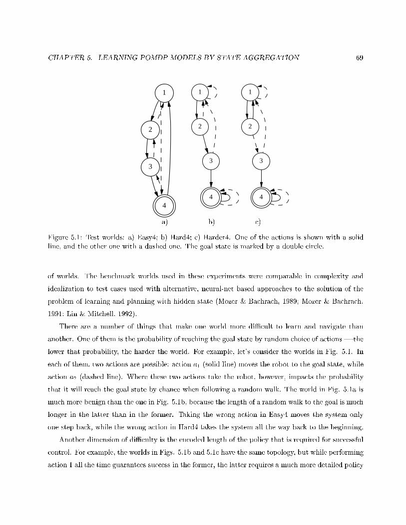
CHAPTER 5. LEARNING POMDP MODELS BY STATE AGGREGATION 69
1
2
4
3
1
2
3
4
1
2
3
4
a) b) c)
Figure 5.1: Test worlds: a) Easy4; b) Hard4; c) Harder4. One of the actions is shown with a solidline, and the other one with a dashed one. The goal state is marked by a double circle.
of worlds. The benchmark worlds used in these experiments were comparable in complexity and
idealization to test cases used with alternative, neural-net based approaches to the solution of the
problem of learning and planning with hidden state (Mozer & Bachrach, 1989; Mozer & Bachrach,
1991; Lin & Mitchell, 1992).
There are a number of things that make one world more diÆcult to learn and navigate than
another. One of them is the probability of reaching the goal state by random choice of actions | the
lower that probability, the harder the world. For example, let's consider the worlds in Fig. 5.1. In
each of them, two actions are possible: action a1 (solid line) moves the robot to the goal state, while
action a2 (dashed line). Where these two actions take the robot, however, impacts the probability
that it will reach the goal state by chance when following a random walk. The world in Fig. 5.1a is
much more benign than the one in Fig. 5.1b, because the length of a random walk to the goal is much
longer in the latter than in the former. Taking the wrong action in Easy4 moves the system only
one step back, while the wrong action in Hard4 takes the system all the way back to the beginning.
Another dimension of diÆculty is the encoded length of the policy that is required for successful
control. For example, the worlds in Figs. 5.1b and 5.1c have the same topology, but while performing
action 1 all the time guarantees success in the former, the latter requires a much more detailed policy
CHAPTER 5. LEARNING POMDP MODELS BY STATE AGGREGATION 70
that depends strongly on the state the POMDP is in. A third dimension is the size of the world, which
directly in uences the diÆculty of reasoning, planning, and learning. A related variable condition is
the length of the action-observation sequence that the agent has available | the larger the world,
the longer a sequence will be required to capture its dynamics. Finally, the degree of perceptual
aliasing in the world would substantially a�ect the agent's ability to learn a description of it and use
that description in planning.
In order to test the performance of the planners and learning algorithms and the in uence of
the variable conditions described above, a number of experiments were performed, whose results are
reported below. The four planners and four learning methods were tested on a total of fourteen
worlds. There were only eight distinct transition diagrams, six of which for the worlds Easy, Hard,
and Harder, with either four or eight states. Both aliased and non-aliased versions were tested. Two
actions existed in each of these twelve worlds. The di�erence between these worlds is the probability
that a random choice of actions would reach the goal. The Easy world is very benign in that random
actions are very likely to succeed. The Hard and Harder worlds are very punishing, because at
each step a wrong action takes the agent back to the state farthest from the goal. The di�erence
between Hard and Harder is that in Hard the correct policy is to always take action one, no matter
what percepts are observed, while in Harder the correct action depends strongly on the state the
agent is in, which can be identi�ed only by observing percepts. The agent can observe the state
number, except if aliasing is introduced, in which case states one and two emit the same percept. All
transitions are deterministic. The combination of the three types of transition patterns (Easy, Hard,
Harder), two sizes of state space (4 and 8 states), and presence or absence of perceptual aliasing
results in a total of twelve experimental POMDP models.
In addition to these twelve worlds, two more POMDP models, Gold 6 and Gold 12, represent
scenarios where a robot has to �nd a piece of gold in one room and carry it to a speci�c goal room.
Gold 6 has two rooms and hence six states (the gold can be in either room or carried by the robot);
Gold 12 has three rooms and twelve states. Four actions are possible | movement in two directions,
clockwise and counterclockwise, as well as grasping and dropping the piece of gold. The robot can
perceive the room number and whether the piece of gold is either in the room, not in the room, or in
its hand. Hence, a total of six percepts can be observed in Gold 6 and nine in Gold 12, which makes
the former world fully observable, while the latter is aliased. A human placed in the Gold 12 world
would �rst plan to �nd the gold, and then carry it to the goal. However, the planners considered
CHAPTER 5. LEARNING POMDP MODELS BY STATE AGGREGATION 71
here cannot plan to perform actions just in order to change their belief state, which makes this world
hard for them.
Each of the worlds has one goal state, and the results are averaged for all possible starting states.
The cumulative discounted reward had a discount factor = 0:9. If a planner could not achieve the
goal within 250 steps, the run was terminated and zero award was given.
Before discussing how planners use the learned model, however, the question about �nding out
which of the learned states is the goal has to be addressed. Both assumptive planning and the MDP-
based strategies need a goal state | either to terminate the iterative deepening search for assumptive
planning, or to construct a proper reward function for the MDP-based algorithms. However, when
a POMDP is learned, it is not clear which of its states correspond to the true goal states in the real
world; in general, there won't be one-to-one correspondence between learned and true states at all.
This circumstance changes signi�cantly the goal criterion used for planning.
One possibility is to transfer the goal from the state domain to the perceptual domain, that is,
instead of trying to reach a goal location, the agent tries to observe the percept that corresponded to
that location in the training exploration trace. For assumptive planning, the states of the FSA that
is an idealized representation of the learned POMDP can be labeled with the most likely percept to
be observed in that state. A solution exists for the MDP-based planners as well. Instead of assigning
reward one to the goal state and zero to all other states, the reward for each state can be equal to
the probability that the goal percept will be observed in this state. It is assumed that the goal state
always emits the goal percept in all test worlds. Thus, a policy that maximizes reward will in e�ect
maximize the probability that the goal percept is seen; if the system is at the goal location each time
the goal percept is seen, this policy will also maximize the probability of reaching the goal state.
The MDP-based planners solved the underlying MDP of the learned POMDP by Q-learning,
sweeping each state in turn and sampling successive states according to the transition probabilities
of the MDP. Learning rate � = 0:1 and discounting factor = 0:9 were used, for a total of 1000
sweeps. Each experiment used a sequence of 200 observations.
Closely following the methodology of (Cassandra et al., 1996), Tables 5.1 through 5.4 show the
discounted cumulative reward for achieving the true goal state averaged over each initial state for
fourteen worlds, four learning methods, and four planners. Average results across planners are shown
as well. The achieved reward for random actions is listed as a baseline for comparison. The name
of each world consists of its transition pattern, number of states, whether there was perceptual
CHAPTER 5. LEARNING POMDP MODELS BY STATE AGGREGATION 72
aliasing (AL) or not (NA), and the number of steps in the exploration sequence. Each number is the
mean over ten trials, and the variances from these trials are used to test for statistically signi�cant
di�erences between performances. All combinations of learning and planning methods were tested
against random choice of actions | the results that were signi�cantly better than random walk at
the 5% error level are shown in bold. It can be claimed that in these cases the learner/planner
did indeed learn an appropriate model of the world and uses the learned model to choose actions
deliberately.
For comparison purposes, Table 5.5 shows the performance of the planners when they have been
supplied with the true POMDP model that generated the data. It can be seen that with very rare
exceptions, all planners achieve the maximal award possible in the respective worlds, which con�rms
their almost perfect ability to plan given the right model. (The only exception is the aliased version
of the Harder 4 world, for which three of the four planners fail to achieve reward better than that
resulting from random actions.) Thus, di�erences between the maximal and achieved awards in
Tables 5.1 through 5.4 can be attributed almost completely to the performance of the learning
methods, which acquire POMDP models from observation data.
The results con�rm the expectation that our ranking of the worlds as easy, hard, and harder is
justi�ed | the harder the world, the larger the di�erence between the maximal and achieved rewards.
Furthermore, the results suggest that none of the learning algorithms is able to take advantage of
the full observability of the non-aliased worlds. The results in Table 5.5 show that if any planner is
given the correct POMDP model, the resulting policy will always result in equal or higher reward
for the non-aliased world than for its aliased counterpart. At the same time, if the models are
learned, approximately half of the time (11 out of 24 cases) higher reward would be achieved in the
aliased variant of the world. This suggests that none of the learning algorithms can take advantage
of a possible full-observability, and instead they learn aliased POMDPs even of fully-observable
environments.
5.4 Experimental Comparison between BW, SGA, BFMM, and
SMTC on Restricted Mobile Robot Navigation
The experiments in the previous section were on purely synthetic POMDPs, while we are interested
mainly in how the considered algorithms would perform on robotic tasks. In order to verify this, the
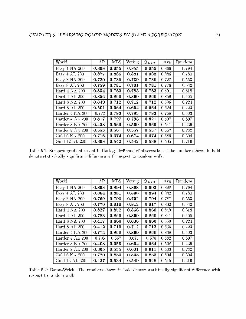
CHAPTER 5. LEARNING POMDP MODELS BY STATE AGGREGATION 73
World AP MLS Voting QMDP Avg Random
Easy 4 NA 200 0.898 0.855 0.855 0.855 0.866 0.794
Easy 4 AL 200 0.877 0.885 0.881 0.903 0.886 0.780
Easy 8 NA 200 0.720 0.730 0.730 0.730 0.728 0.553
Easy 8 AL 200 0.759 0.781 0.781 0.781 0.776 0.542
Hard 4 NA 200 0.854 0.783 0.783 0.783 0.801 0.618
Hard 4 AL 200 0.856 0.860 0.860 0.860 0.859 0.605
Hard 8 NA 200 0.649 0.712 0.712 0.712 0.696 0.224
Hard 8 AL 200 0.501 0.664 0.664 0.664 0.624 0.223
Harder 4 NA 200 0.722 0.783 0.783 0.783 0.768 0.603
Harder 4 AL 200 0.817 0.797 0.793 0.821 0.807 0.597
Harder 8 NA 200 0.458 0.569 0.569 0.569 0.541 0.239
Harder 8 AL 200 0.553 0.561 0.557 0.557 0.557 0.232
Gold 6 NA 200 0.716 0.674 0.674 0.674 0.685 0.304
Gold 12 AL 200 0.398 0.542 0.542 0.538 0.505 0.216
Table 5.1: Steepest gradient ascent in the log-likelihood of observations. The numbers shown in bolddenote statistically signi�cant di�erence with respect to random walk.
World AP MLS Voting QMDP Avg Random
Easy 4 NA 200 0.898 0.894 0.898 0.903 0.898 0.794
Easy 4 AL 200 0.864 0.881 0.890 0.894 0.882 0.780
Easy 8 NA 200 0.769 0.793 0.792 0.794 0.787 0.553
Easy 8 AL 200 0.770 0.810 0.813 0.817 0.802 0.542
Hard 4 NA 200 0.827 0.852 0.856 0.860 0.849 0.618
Hard 4 AL 200 0.783 0.860 0.860 0.860 0.841 0.605
Hard 8 NA 200 0.417 0.606 0.606 0.606 0.559 0.224
Hard 8 AL 200 0.412 0.710 0.712 0.712 0.636 0.223
Harder 4 NA 200 0.773 0.860 0.860 0.860 0.838 0.603
Harder 4 AL 200 0.705 0.667 0.678 0.678 0.682 0.597
Harder 8 NA 200 0.408 0.655 0.664 0.664 0.598 0.239
Harder 8 AL 200 0.365 0.555 0.601 0.611 0.533 0.232
Gold 6 NA 200 0.720 0.833 0.833 0.833 0.804 0.304
Gold 12 AL 200 0.427 0.534 0.549 0.548 0.515 0.216
Table 5.2: Baum-Welch. The numbers shown in bold denote statistically signi�cant di�erence withrespect to random walk.
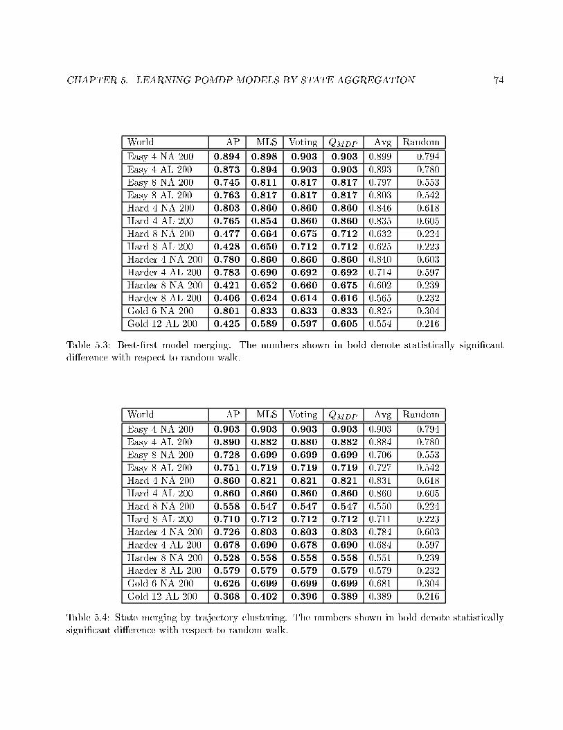
CHAPTER 5. LEARNING POMDP MODELS BY STATE AGGREGATION 74
World AP MLS Voting QMDP Avg Random
Easy 4 NA 200 0.894 0.898 0.903 0.903 0.899 0.794
Easy 4 AL 200 0.873 0.894 0.903 0.903 0.893 0.780
Easy 8 NA 200 0.745 0.811 0.817 0.817 0.797 0.553
Easy 8 AL 200 0.763 0.817 0.817 0.817 0.803 0.542
Hard 4 NA 200 0.803 0.860 0.860 0.860 0.846 0.618
Hard 4 AL 200 0.765 0.854 0.860 0.860 0.835 0.605
Hard 8 NA 200 0.477 0.664 0.675 0.712 0.632 0.224
Hard 8 AL 200 0.428 0.650 0.712 0.712 0.625 0.223
Harder 4 NA 200 0.780 0.860 0.860 0.860 0.840 0.603
Harder 4 AL 200 0.783 0.690 0.692 0.692 0.714 0.597
Harder 8 NA 200 0.421 0.652 0.660 0.675 0.602 0.239
Harder 8 AL 200 0.406 0.624 0.614 0.616 0.565 0.232
Gold 6 NA 200 0.801 0.833 0.833 0.833 0.825 0.304
Gold 12 AL 200 0.425 0.589 0.597 0.605 0.554 0.216
Table 5.3: Best-�rst model merging. The numbers shown in bold denote statistically signi�cantdi�erence with respect to random walk.
World AP MLS Voting QMDP Avg Random
Easy 4 NA 200 0.903 0.903 0.903 0.903 0.903 0.794
Easy 4 AL 200 0.890 0.882 0.880 0.882 0.884 0.780
Easy 8 NA 200 0.728 0.699 0.699 0.699 0.706 0.553
Easy 8 AL 200 0.751 0.719 0.719 0.719 0.727 0.542
Hard 4 NA 200 0.860 0.821 0.821 0.821 0.831 0.618
Hard 4 AL 200 0.860 0.860 0.860 0.860 0.860 0.605
Hard 8 NA 200 0.558 0.547 0.547 0.547 0.550 0.224
Hard 8 AL 200 0.710 0.712 0.712 0.712 0.711 0.223
Harder 4 NA 200 0.726 0.803 0.803 0.803 0.784 0.603
Harder 4 AL 200 0.678 0.690 0.678 0.690 0.684 0.597
Harder 8 NA 200 0.528 0.558 0.558 0.558 0.551 0.239
Harder 8 AL 200 0.579 0.579 0.579 0.579 0.579 0.232
Gold 6 NA 200 0.626 0.699 0.699 0.699 0.681 0.304
Gold 12 AL 200 0.368 0.402 0.396 0.389 0.389 0.216
Table 5.4: State merging by trajectory clustering. The numbers shown in bold denote statisticallysigni�cant di�erence with respect to random walk.
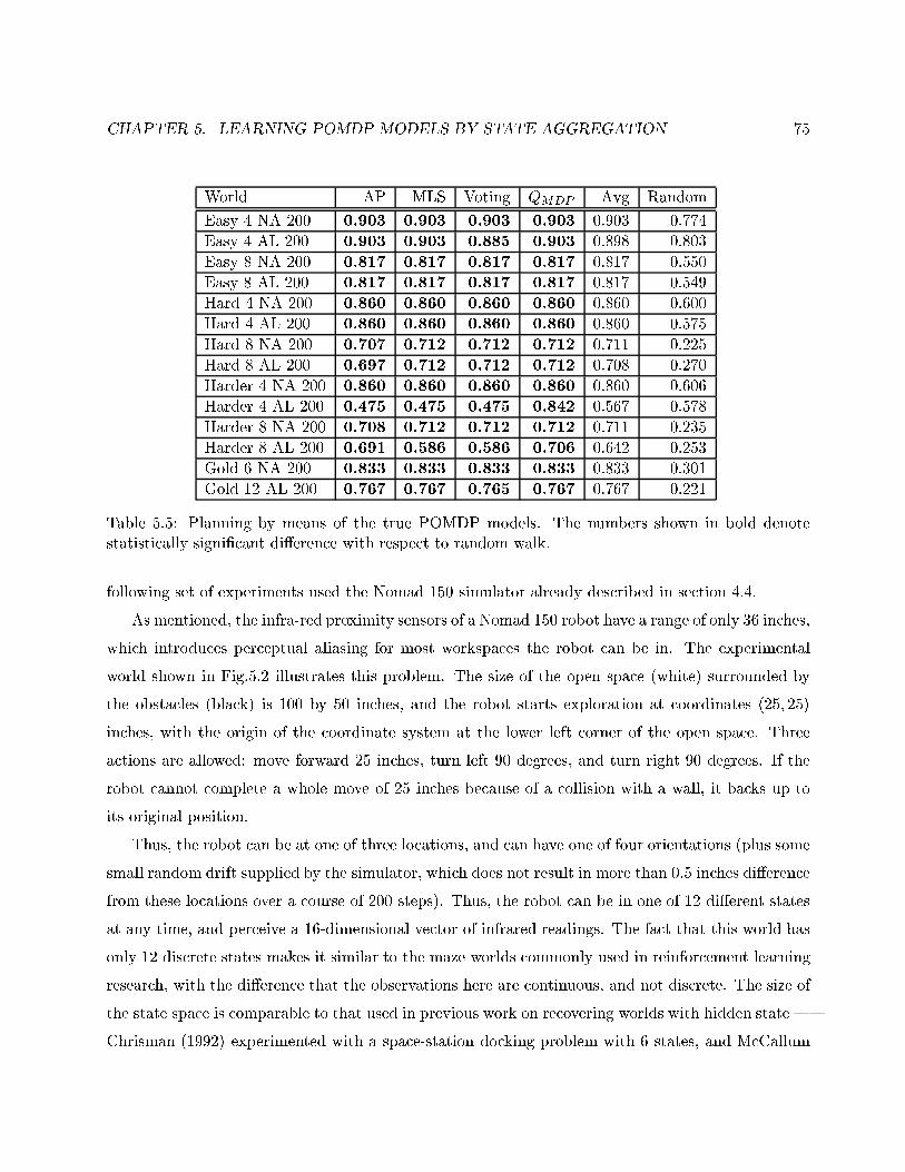
CHAPTER 5. LEARNING POMDP MODELS BY STATE AGGREGATION 75
World AP MLS Voting QMDP Avg Random
Easy 4 NA 200 0.903 0.903 0.903 0.903 0.903 0.774
Easy 4 AL 200 0.903 0.903 0.885 0.903 0.898 0.803
Easy 8 NA 200 0.817 0.817 0.817 0.817 0.817 0.550
Easy 8 AL 200 0.817 0.817 0.817 0.817 0.817 0.549
Hard 4 NA 200 0.860 0.860 0.860 0.860 0.860 0.600
Hard 4 AL 200 0.860 0.860 0.860 0.860 0.860 0.575
Hard 8 NA 200 0.707 0.712 0.712 0.712 0.711 0.225
Hard 8 AL 200 0.697 0.712 0.712 0.712 0.708 0.270
Harder 4 NA 200 0.860 0.860 0.860 0.860 0.860 0.606
Harder 4 AL 200 0.475 0.475 0.475 0.842 0.567 0.578
Harder 8 NA 200 0.708 0.712 0.712 0.712 0.711 0.235
Harder 8 AL 200 0.691 0.586 0.586 0.706 0.642 0.253
Gold 6 NA 200 0.833 0.833 0.833 0.833 0.833 0.301
Gold 12 AL 200 0.767 0.767 0.765 0.767 0.767 0.221
Table 5.5: Planning by means of the true POMDP models. The numbers shown in bold denotestatistically signi�cant di�erence with respect to random walk.
following set of experiments used the Nomad 150 simulator already described in section 4.4.
As mentioned, the infra-red proximity sensors of a Nomad 150 robot have a range of only 36 inches,
which introduces perceptual aliasing for most workspaces the robot can be in. The experimental
world shown in Fig.5.2 illustrates this problem. The size of the open space (white) surrounded by
the obstacles (black) is 100 by 50 inches, and the robot starts exploration at coordinates (25; 25)
inches, with the origin of the coordinate system at the lower left corner of the open space. Three
actions are allowed: move forward 25 inches, turn left 90 degrees, and turn right 90 degrees. If the
robot cannot complete a whole move of 25 inches because of a collision with a wall, it backs up to
its original position.
Thus, the robot can be at one of three locations, and can have one of four orientations (plus some
small random drift supplied by the simulator, which does not result in more than 0:5 inches di�erence
from these locations over a course of 200 steps). Thus, the robot can be in one of 12 di�erent states
at any time, and perceive a 16-dimensional vector of infrared readings. The fact that this world has
only 12 discrete states makes it similar to the maze worlds commonly used in reinforcement learning
research, with the di�erence that the observations here are continuous, and not discrete. The size of
the state space is comparable to that used in previous work on recovering worlds with hidden state |
Chrisman (1992) experimented with a space-station docking problem with 6 states, and McCallum
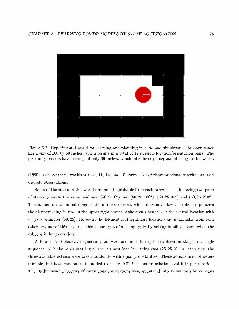
CHAPTER 5. LEARNING POMDP MODELS BY STATE AGGREGATION 76
Figure 5.2: Experimental world for learning and planning in a Nomad simulator. The open spacehas a size of 100 by 50 inches, which results in a total of 12 possible location/orientation pairs. Theproximity sensors have a range of only 36 inches, which introduces perceptual aliasing in this world.
(1995) used synthetic worlds with 8, 11, 14, and 15 states. All of these previous experiments used
discrete observations.
Some of the states in this world are indistinguishable from each other | the following two pairs
of states generate the same readings: (50; 25; 0o) and (50; 25; 180o); (50; 25; 90o) and (50; 25; 270o).
This is due to the limited range of the infrared sensors, which does not allow the robot to perceive
the distinguishing feature in the upper right corner of the area when it is at the central location with
(x; y) coordinates (50; 25). However, the leftmost and rightmost locations are identi�able from each
other because of this feature. This is one type of aliasing typically arising in oÆce spaces when the
robot is in long corridors.
A total of 200 observation/action pairs were acquired during the exploration stage in a single
sequence, with the robot starting at the leftmost location facing east (25; 25; 0). At each step, the
three available actions were taken randomly with equal probabilities. These actions are not deter-
ministic, but have random noise added to them: 0:01 inch per translation, and 0:1o per rotation.
The 16-dimensional vectors of continuous observations were quantized into 12 symbols by k-means
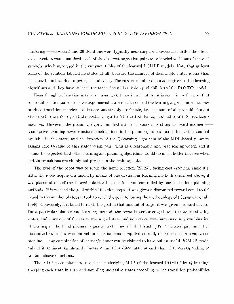
CHAPTER 5. LEARNING POMDP MODELS BY STATE AGGREGATION 77
clustering | between 5 and 20 iterations were typically necessary for convergence. After the obser-
vation vectors were quantized, each of the observation/action pairs were labeled with one of these 12
symbols, which were used in the emission tables of the learned POMDP models. Note that at least
some of the symbols labeled no states at all, because the number of discernible states is less than
their total number, due to perceptual aliasing. The correct number of states is given to the learning
algorithms and they have to learn the transition and emission probabilities of the POMDP model.
Even though each action is tried on average 6 times in each state, it is sometimes the case that
some state/action pairs are never experienced. As a result, some of the learning algorithms sometimes
produce transition matrices, which are not strictly stochastic, i.e. the sum of all probabilities out
of a certain state for a particular action might be 0 instead of the required value of 1 for stochastic
matrices. However, the planning algorithms deal with such cases in a straightforward manner |
assumptive planning never considers such actions in the planning process, as if this action was not
available in this state, and the iteration of the Q-learning algorithm of the MDP-based planners
assigns zero Q-value to this state/action pair. This is a reasonable and practical approach and it
cannot be expected that other learning and planning algorithms would do much better in cases when
certain transitions are simply not present in the training data.
The goal of the robot was to reach the home location (25; 25), facing east (steering angle 0o).
After the robot acquired a model by means of one of the four learning methods described above, it
was placed at one of the 12 available starting locations and controlled by one of the four planning
methods. If it reached the goal within 10 action steps, it was given a discounted reward equal to 0:9
raised to the number of steps it took to reach the goal, following the methodology of (Cassandra et al.,
1996). Conversely, if it failed to reach the goal in that amount of steps, it was given a reward of zero.
For a particular planner and learning method, the rewards were averaged over the twelve starting
states, and since one of the states was a goal state and no actions were necessary, any combination
of learning method and planner is guaranteed a reward of at least 1=12. The average cumulative
discounted award for random action selection was computed as well, to be used as a comparison
baseline | any combination of learner/planner can be claimed to have built a useful POMDP model
only if it achieves signi�cantly better cumulative discounted reward than that corresponding to
random choice of actions.
The MDP-based planners solved the underlying MDP of the learned POMDP by Q-learning,
sweeping each state in turn and sampling successive states according to the transition probabilities
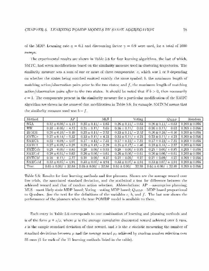
CHAPTER 5. LEARNING POMDP MODELS BY STATE AGGREGATION 78
of the MDP. Learning rate � = 0:1 and discounting factor = 0:9 were used, for a total of 1000
sweeps.
The experimental results are shown in Table 5.6 for four learning algorithms, the last of which,
SMTC, had seven modi�cations based on the similarity measure used in clustering trajectories. The
similarity measure was a sum of one or more of three components: c, which was 1 or 0 depending
on whether the states being matched emitted exactly the same symbol; b, the maximum length of
matching action/observation pairs prior to the two states; and f , the maximum length of matching
action/observation pairs after to the two states. It should be noted that if b > 0, then necessarily
c = 1. The components present in the similarity measure for a particular modi�cation of the SMTC
algorithm are shown in the name of that modi�cation in Table 5.6; for example, SMTCbf means that
the similarity measure used was b+ f .
Method AP MLS Voting QMDP Random
SGA 0:32� 0:06=+ 4:13 0:25� 0:11=� 1:65 0:26� 0:11=� 0:63 0:26� 0:11=� 0:63 0:269� 0:056
BW 0:32� 0:06=+ 4:13 0:25� 0:11=� 1:65 0:26� 0:11=� 0:63 0:26� 0:11=� 0:63 0:269� 0:056
BFMM 0:26� 0:16=� 0:40 0:23� 0:14=� 2:52 0:23� 0:14=� 2:52 0:26� 0:16=� 0:40 0:269� 0:056
SMTCc 0:27� 0:14=+ 0:32 0:33� 0:11=+ 4:23 0:33� 0:11=+ 4:23 0:33� 0:11=+ 4:23 0:269� 0:056
SMTCb 0:22� 0:08=� 4:07 0:17� 0:12=� 7:31 0:17� 0:12=� 7:31 0:17� 0:12=� 7:31 0:269� 0:056
SMTCf 0:27� 0:08=+ 0:28 0:23� 0:18=� 2:29 0:25� 0:17=� 1:46 0:23� 0:18=� 2:37 0:269� 0:056
SMTCcb 0:28� 0:00=+ 0:85 0:28� 0:00=+ 0:85 0:28� 0:00=+ 0:85 0:28� 0:00=+ 0:85 0:269� 0:056
SMTCcf 0:28� 0:01=+ 0:63 0:26� 0:06=� 0:61 0:26� 0:06=� 0:61 0:26� 0:06=� 0:61 0:269� 0:056
SMTCbf 0:20� 0:11=� 5:17 0:21� 0:09=� 4:27 0:21� 0:09=� 4:27 0:21� 0:09=� 4:27 0:269� 0:056
SMTCcbf 0:33� 0:07=+ 4:94 0:33� 0:07=+ 4:94 0:33� 0:07=+ 4:94 0:33� 0:07=+ 4:94 0:269� 0:056
True 0:65� 0:00=+ 32:88 0:65� 0:00=+ 32:88 0:65� 0:00=+ 32:88 0:65� 0:00=+ 32:88 0:269� 0:056
Table 5.6: Results for four learning methods and �ve planners. Shown are the average reward over�ve trials, the associated standard deviation, and the statistical z test for di�erence between theachieved reward and that of random action selection. Abbreviations: AP { assumptive planning;MLS { most-likely state MDP-based; Voting { voting MDP-based; QMDP { MDP-based proportionalto Q-values. See the text for the de�nitions of the variables c, b, and f . The last row shows theperformance of the planners when the true POMDP model is available to them.
Each entry in Table 5.6 corresponds to one combination of learning and planning methods and
is of the form � � s=z, where � is the average cumulative discounted reward achieved over 5 runs,
s is the sample standard deviation of that reward, and z is the z statistic measuring the number of
standard deviations between � and the average award �r achieved by random number selection over
55 runs (5 for each of the 11 learning methods listed in the table).
CHAPTER 5. LEARNING POMDP MODELS BY STATE AGGREGATION 79
The z statistic was computed according to the formula for paired z-tests:
z =�� �r
sp
q1n1
+ 1n2
;
where n1 = 5 is the number of samples, which � was computed from, and n2 = 55 is the number
of samples used for �nding �r. The pooled variance sp was computed as follows:
sp =
s(n1 � 1)s2 + (n2 � 1)s2r
n1 + n2 � 1;
where sr is the sample standard deviation of the performance of random action selection from
the last column of Table 5.6.
The z tests, computed in Table 5.6, make the assumption of Gaussian distributions of the respec-
tive samples. Hence, the computed z values have to be regarded with some caution, because while
the distribution of rewards for random choice of actions is indeed roughly Gaussian, the distribution
of rewards for a pair of a learner and a planner is most typically not. The usual behavior of the robot
during a series of test runs is either to go to the goal directly and achieve maximum reward, if a good
model has been acquired, or to bang obstinately into a wall and get no reward at all. This is due to
the fact that the MDP-based policies and assumptive plans are �xed, and since the belief distribution
converges to a �xed value when the robot is held at the same location, the POMDP policies are in
practice �xed as well and if they are wrong, the robot cannot escape that location. Consequently, the
rewards are distributed towards the extremes, which violates the Gaussian requirement for z-tests.
With this cautionary note in mind, the results from Table 5.6 can be interpreted to indicate
that the following combinations of learning and planning methods achieve performance signi�cantly
better than random action selection: SGA/AP, BW/AP, SMTCc with all MDP-based planners,
and SMTCcbf with all planners. The version of SMTC, which employs the sum of all matching
components (SMTCcbf) performs best, which con�rms expectations. However, those versions of
SMTC, which use the backward matching distance b, but not the direct match c, perform very
badly, even though if b > 0, c = 1, as mentioned above.
By considering the statistical distribution of rewards achieved by these algorithms, we can gain
understanding of why some algorithms are more successful than others. In practice, the higher result
of SMTC comes from that fact that it manages to recover the true POMDP model more often than
CHAPTER 5. LEARNING POMDP MODELS BY STATE AGGREGATION 80
the other algorithms, and when it recovers it, the model is deterministic. Due to the nature of the
iterative algorithms, it is virtually impossible for them to produce a deterministic POMDP model,
which probably hurts the performance of the planners when they use such a model later. So, it is
not a matter of what models SMTC learns (when successful, they are always perfect), but of how
often it produces the perfect model.
For the sake of comparison, the last line of Table 5.6 lists the performance of the four planners
when they have a fully observable model of the world (still represented as a POMDP, but each of
whose states always emits the same unique observation). It is evident that all planners always �nd
the optimal plan in this world, which suggests that whenever a combination of a learning and a
planning method achieves suboptimal results, this is most likely due to acquiring a wrong model on
the part of the learner rather than on failure to use the model correctly. It can be seen that while at
least some of the learning methods achieve performance statistically signi�cantly better than random
action selection, they are still far from recovering reliably a POMDP model of even such a simple
test environment.
In addition to converging to suboptimal local maxima in likelihood, another likely reason why
learning in these experiments did not recover perfectly the correct POMDP model is the nature of
the exploration policy. Essentially, the robot was following a random walk in its workspace, which
provides for only very uneven and partial coverage. Furthermore, random walk is a completely
undirected and hence very slow method of obtaining training data, which is very undesirable for
operation on real robots. The next chapter, which discusses the implementation of a state-merging
algorithm on a real mobile robot, follows a more directed and constrained exploration policy in order
to improve the sample eÆciency of collecting training data and learning from them.
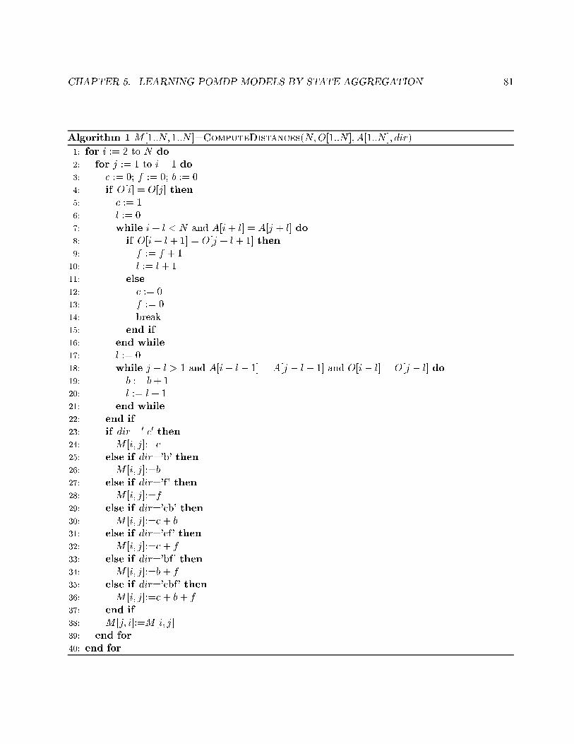
CHAPTER 5. LEARNING POMDP MODELS BY STATE AGGREGATION 81
Algorithm 1 M [1::N; 1::N ]=ComputeDistances(N;O[1::N ]; A[1::N ]; dir)
1: for i := 2 to N do
2: for j := 1 to i� 1 do3: c := 0; f := 0; b := 04: if O[i] = O[j] then5: c := 16: l := 07: while i+ l < N and A[i+ l] = A[j + l] do8: if O[i+ l + 1] = O[j + l + 1] then9: f := f + 1
10: l := l + 111: else
12: c := 013: f := 014: break15: end if
16: end while
17: l := 018: while j � l > 1 and A[i� l � 1] = A[j � l � 1] and O[i� l] = O[j � l] do19: b := b+ 120: l := l + 121: end while
22: end if
23: if dir =0 c0 then
24: M [i; j]:=c25: else if dir='b' then26: M [i; j]:=b27: else if dir='f' then28: M [i; j]:=f29: else if dir='cb' then30: M [i; j]:=c + b
31: else if dir='cf' then32: M [i; j]:=c + f
33: else if dir='bf' then34: M [i; j]:=b + f
35: else if dir='cbf' then36: M [i; j]:=c + b+ f
37: end if
38: M [j; i]:=M [i; j]39: end for
40: end for
Chapter 6
Constrained Trajectory Clustering for
Mobile Robot Localization
The experiments in the previous chapter suggest that probabilistic models can successfully be learned
by merging states on the basis of trajectory matches. This chapter discusses how this idea can be
implemented on real robots, which are only equipped with a minimal number of inexpensive sensors
and motors. The �rst problem we address is the need for revision of the exploration policy of the
robot. The revised policy is implemented by means of a wall-following controller and is used to
explore the outer perimeter of an environment. This allows for exhaustive search of the model
structure to be performed, which reduces the state-merging algorithm from the previous chapter to
a search for the period of circling of the robot along its perimeter. This search is performed very
eÆciently on-board a simple di�erential-drive mobile robot with three infrared proximity sensors and
a digital compass, and the resulting model is used successfully for self-localization.
6.1 Space Exploration Policies for Mobile Robots
As described above, we are considering the scenario when the robot accumulates an execution trace
while following an exploration policy, and after that constructs a POMDP from this execution trace.
However, the exploration policy described in the previous chapter has a serious de�ciency as regards
its implementation on real robots: trying random actions in each state does not provide for complete
and eÆcient coverage of the robot's workspace. In practice, the robot follows a random walk, which
82
CHAPTER 6. CONSTRAINED TRAJECTORYCLUSTERING FORMOBILE ROBOT LOCALIZATION83
tends to cover its workspace very unevenly, and often fails to visit large regions.
The eÆcient and complete covering of an unknown space by a mobile robot is a hard problem in
itself, and has been researched extensively due to its practical signi�cance for many robotic applica-
tions such as automated lawn mowing, harvesting, oor cleaning, mine hunting, etc. (Choset, 2001).
Many exact solutions based on cellular decomposition have been proposed for the easiest case, when
a full map of the environment is given (Latombe, 1991; Zelinsky, 1991; Zelinsky, 1992). However,
we are explicitly interested in the case when no such map is available. When the environment is un-
known, but the robot still has full knowledge of its coordinates, a number of algorithms can be used.
Hert et al. (1996) proposed a solution based on partial discretization of space where the width of the
cells is �xed, but the top and bottom can have any shape. The CCR algorithm due to Butler (1998)
uses reactive construction and no time-based history to perform coverage, and has been proven to
be complete. These algorithms do not use an incrementally built map and hence are very suitable
for an exploration policy which is executed before any model learning is performed. However, they
cannot be used for the scenario we are considering, because they rely on complete knowledge of the
robot's coordinates at any moment in time.
The only known strategies that can handle the hardest case of exploring completely unknown
environments without knowledge of the true coordinates of the exploring robot are based on ap-
proximate cellular decompositions, where the unknown environment is represented by a discrete
occupancy grid, in conjunction with simultaneous localization and mapping algorithms. If a global
occupancy grid is learned incrementally as the the robot explores its environment, a direct method
to achieve full coverage is to give unexplored cells as goals to a planning algorithm which operates
on the occupancy grid (map) extracted so far (Thrun et al., 1998a). It can easily be seen that this
method would completely explore the environment, up to the resolution of the grid. As noted in the
Problem Statement (Section 1.2), however, we are interested in exploration policies which do not use
intermediate learned models, and furthermore, the class of robots we are considering does not allow
global occupancy grids to be learned.
Another approach is to explore only the part of the environment that is accessible by following one
or more simple exploration behaviors. Kuipers and Byun (1991) considered an exploration strategy,
which consists of a sequence of the following four behaviors: Follow-the-Midline, Move-along-Object-
on-Right, Move-along-Object-on-Left, and Blind-Step. This is also the general approach we have
followed in our experiments, where the chosen task is such that the robot can reliably explore a
CHAPTER 6. CONSTRAINED TRAJECTORYCLUSTERING FORMOBILE ROBOT LOCALIZATION84
part of its workspace by following a non-planning exploration policy that does not have to use any
internal representations.
6.2 Experimental Task
Nehmzow and Smithers (1992) and Matari�c (1992) considered the task of self-localization of a robot
along the inner perimeter of its environment. The objective of the robot is to build an internal
representation of this perimeter and be able to determine its position by means of this internal
representation. It is desirable to have as high spatial resolution as possible, while at the same
time maintaining high accuracy of localization. These two requirements are contradictory, because
increasing the number of distinguishable states also increases the chance of erroneous localization.
Nehmzow and Smithers used a spreading-activation Kohonen neural network with a �xed number
of nodes (neurons) as a world model. The weights of this network were updated in the process of
learning a model of the environment. They used the output of the motors of the robot, instead of
sensory input, to train the neural net. The biggest limitation of their approach is the �xed number of
nodes in the model, and thus the resulting limited spatial resolution during localization. In fact, even
though they started with a neural net of 50 nodes, the robot could ultimately distinguish only 11
locations, mostly corners of the inner perimeter of the robot's environment (Nehmzow & Smithers,
1992).
The limited spatial resolution is the main problem with Matari�c's approach, too (Matari�c, 1992).
She chose three large, stable, and reliably detectable landmark types: left walls, right walls, and
corridors, along with a default landmark type for irregular boundaries. While the chosen set of
landmarks resulted in reliable position tracking, the robot was inherently incapable of determining
where it was along a particular wall or a corridor, for example. The objective of our implementation
of a state-merging learning algorithm is to eliminate the limited spatial resolution resulting from the
approaches described above.
In particular, it would be desirable to reduce the limited spatial resolution of the localization
process down to an accuracy of ten centimeters. This would be very useful, for example, in the
scenario when an unmanned vehicle has to move loads between work cells that are located along the
walls of a workshop. If the vehicle is only able to identify corners and stop there, as in (Nehmzow
& Smithers, 1992), or only walls it is aligned with, as in (Matari�c, 1992), such an accuracy would
CHAPTER 6. CONSTRAINED TRAJECTORYCLUSTERING FORMOBILE ROBOT LOCALIZATION85
be insuÆcient for loading and unloading cargo. However, if the accuracy of localization is under
ten centimeters, loading and unloading is much easier. This is also the typical localization accuracy
achieved by methods based on global occupancy grids. The following sections describe how this can
be done with only minimal expenses in sensors and computational power.
6.3 Experimental Robot and Low-Level Control
For our experiments, we built a simple mobile robot with two di�erential-drive wheels and a passive
caster, three IR sensors, and a digital compass (Fig. 6.1). The �rst IR sensor (IR1) points forward,
while IR2 points to the right and is placed in front of the right wheel, and IR3 also points to the
right, but is placed behind the right wheel (Fig. 6.2). The robot is controlled by a Palm Pilot III
palm-held computer with a Motorola DragonBall CPU (clock rate 16MHz), running PalmOS 3.1.
The control step, including the time to record the sensor readings in a log �le, is 290ms. The robot
is also supplied with a Dinsmore digital compass, which senses the local magnetic �eld and has a
resolution of 45o (eight directions).
The exploration of the inner perimeter can be implemented by means of a low-level wall-following
controller which has no state information and uses only the current readings of the infrared proximity
sensors as \whiskers" in a fast control loop in order to correct the movement of the robot. Depending
on the number of sensors available, several approaches are possible. If a full sonar or IR ring is
available, so that several sensors can measure the distance to the wall, a straight line �tted to these
readings would give the direction of the wall with respect to the robot's orientation, as well as the
distance to the wall from the robot. Then, a PID controller can be used to minimize the deviation
of that distance from a pre-speci�ed value.
Fitting a line is not possible when there is only one proximity sensor. This method is also very
unreliable when there are only two sensors which, however, have a lot of noise. Even moderate
amounts of noise in readings could result in huge errors in the estimated angle and distance to the
wall. A better approach for such cases is to build an observer which uses a Kalman �lter to aggregate
multiple sensor readings and reconcile them with the change in the wall's position resulting from the
motion of the robot (van Turennout et al., 1992; Yata et al., 1998). This approach, however, requires
the availability of a reasonably good model of the motion of the robot and/or odometry readings,
which our experimental robot lacks. Furthermore, propagating the error in vehicle odometry is not
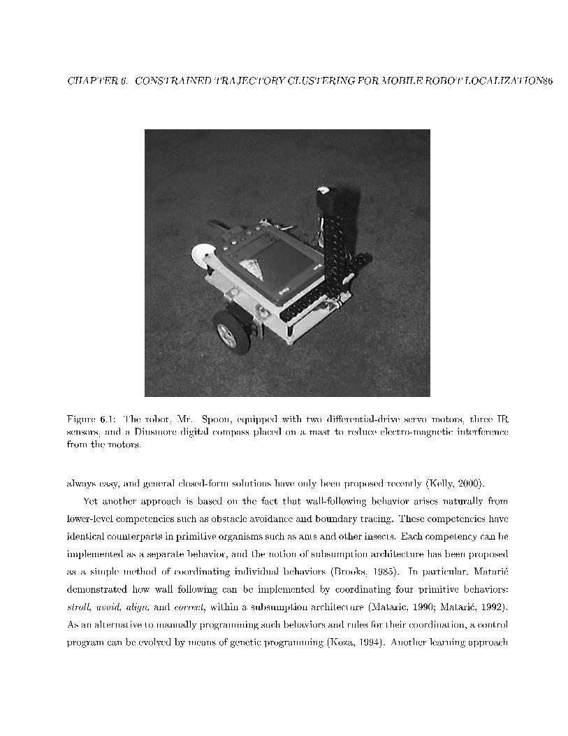
CHAPTER 6. CONSTRAINED TRAJECTORYCLUSTERING FORMOBILE ROBOT LOCALIZATION86
Figure 6.1: The robot, Mr. Spoon, equipped with two di�erential-drive servo motors, three IRsensors, and a Dinsmore digital compass placed on a mast to reduce electro-magnetic interferencefrom the motors.
always easy, and general closed-form solutions have only been proposed recently (Kelly, 2000).
Yet another approach is based on the fact that wall-following behavior arises naturally from
lower-level competencies such as obstacle avoidance and boundary tracing. These competencies have
identical counterparts in primitive organisms such as ants and other insects. Each competency can be
implemented as a separate behavior, and the notion of subsumption architecture has been proposed
as a simple method of coordinating individual behaviors (Brooks, 1985). In particular, Matari�c
demonstrated how wall following can be implemented by coordinating four primitive behaviors:
stroll, avoid, align, and correct, within a subsumption architecture (Mataric, 1990; Matari�c, 1992).
As an alternative to manually programming such behaviors and rules for their coordination, a control
program can be evolved by means of genetic programming (Koza, 1994). Another learning approach
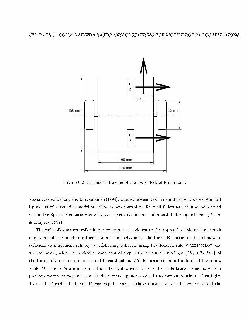
CHAPTER 6. CONSTRAINED TRAJECTORYCLUSTERING FORMOBILE ROBOT LOCALIZATION87
150 mm
IR 1
IR2
IR3
100 mm
170 mm
55 mm
Figure 6.2: Schematic drawing of the lower deck of Mr. Spoon.
was suggested by Law and Miikkulainen (1994), where the weights of a neural network were optimized
by means of a genetic algorithm. Closed-loop controllers for wall following can also be learned
within the Spatial Semantic Hierarchy, as a particular instance of a path-following behavior (Pierce
& Kuipers, 1997).
The wall-following controller in our experiments is closest to the approach of Matari�c, although
it is a monolithic function rather than a set of behaviors. The three IR sensors of the robot were
suÆcient to implement reliably wall-following behavior using the decision rule WallFollow de-
scribed below, which is invoked at each control step with the current readings fIR1; IR2; IR3g of
the three infra-red sensors, measured in centimeters. IR1 is measured from the front of the robot,
while IR2 and IR3 are measured from its right wheel. This control rule keeps no memory from
previous control steps, and controls the motors by means of calls to four subroutines: TurnRight,
TurnLeft, TurnHardLeft, and MoveStraight. Each of these routines drives the two wheels of the
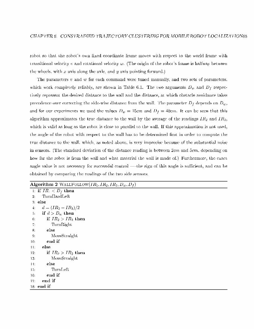
CHAPTER 6. CONSTRAINED TRAJECTORYCLUSTERING FORMOBILE ROBOT LOCALIZATION88
robot so that the robot's own �xed coordinate frame moves with respect to the world frame with
transitional velocity v and rotational velocity !. (The origin of the robot's frame is halfway between
the wheels, with x axis along the axle, and y axis pointing forward.)
The parameters v and w for each command were tuned manually, and two sets of parameters,
which work completely reliably, are shown in Table 6.1. The two arguments Dw and Df respec-
tively represent the desired distance to the wall and the distance, at which obstacle avoidance takes
precedence over correcting the side-wise distance from the wall. The parameter Df depends on Dw,
and for our experiments we used the values Dw = 15cm and Df = 40cm. It can be seen that this
algorithm approximates the true distance to the wall by the average of the readings IR2 and IR3,
which is valid as long as the robot is close to parallel to the wall. If this approximation is not used,
the angle of the robot with respect to the wall has to be determined �rst in order to compute the
true distance to the wall, which, as noted above, is very imprecise because of the substantial noise
in sensors. (The standard deviation of the distance reading is between 2cm and 5cm, depending on
how far the robot is from the wall and what material the wall is made of.) Furthermore, the exact
angle value is not necessary for successful control | the sign of this angle is suÆcient, and can be
obtained by comparing the readings of the two side sensors.
Algorithm 2 WallFollow(IR1; IR2; IR3;Dw;Df)
1: if IR1 < Df then
2: TurnHardLeft3: else
4: d = (IR2 + IR3)=25: if d > Dw then
6: if IR2 > IR3 then
7: TurnRight8: else
9: MoveStraight10: end if
11: else
12: if IR2 > IR3 then
13: MoveStraight14: else
15: TurnLeft16: end if
17: end if
18: end if
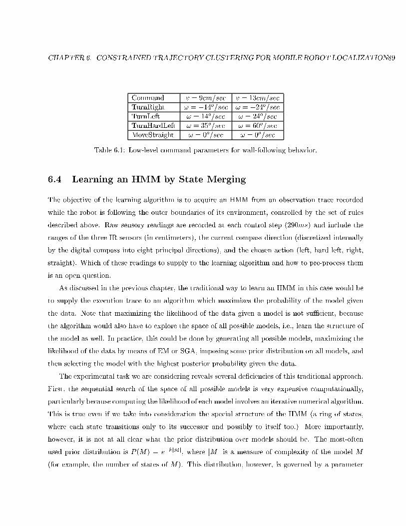
CHAPTER 6. CONSTRAINED TRAJECTORYCLUSTERING FORMOBILE ROBOT LOCALIZATION89
Command v = 9cm=sec v = 13cm=sec
TurnRight ! = �14o=sec ! = �24o=sec
TurnLeft ! = 14o=sec ! = 24o=sec
TurnHardLeft ! = 35o=sec ! = 60o=sec
MoveStraight ! = 0o=sec ! = 0o=sec
Table 6.1: Low-level command parameters for wall-following behavior.
6.4 Learning an HMM by State Merging
The objective of the learning algorithm is to acquire an HMM from an observation trace recorded
while the robot is following the outer boundaries of its environment, controlled by the set of rules
described above. Raw sensory readings are recorded at each control step (290ms) and include the
ranges of the three IR sensors (in centimeters), the current compass direction (discretized internally
by the digital compass into eight principal directions), and the chosen action (left, hard left, right,
straight). Which of these readings to supply to the learning algorithm and how to pre-process them
is an open question.
As discussed in the previous chapter, the traditional way to learn an HMM in this case would be
to supply the execution trace to an algorithm which maximizes the probability of the model given
the data. Note that maximizing the likelihood of the data given a model is not suÆcient, because
the algorithm would also have to explore the space of all possible models, i.e., learn the structure of
the model as well. In practice, this could be done by generating all possible models, maximizing the
likelihood of the data by means of EM or SGA, imposing some prior distribution on all models, and
then selecting the model with the highest posterior probability given the data.
The experimental task we are considering reveals several de�ciencies of this traditional approach.
First, the sequential search of the space of all possible models is very expensive computationally,
particularly because computing the likelihood of each model involves an iterative numerical algorithm.
This is true even if we take into consideration the special structure of the HMM (a ring of states,
where each state transitions only to its successor and possibly to itself too.) More importantly,
however, it is not at all clear what the prior distribution over models should be. The most-often
used prior distribution is P (M) = e�kjM j, where jM j is a measure of complexity of the model M
(for example, the number of states of M). This distribution, however, is governed by a parameter
CHAPTER 6. CONSTRAINED TRAJECTORYCLUSTERING FORMOBILE ROBOT LOCALIZATION90
k which speci�es the relative weight of the log-likelihood lnP (DjM) and log-prior lnP (M), and it
is not clear what value of k should be chosen. Uniform prior distribution is not acceptable either,
because the model that has one state per observation would always have the maximal likelihood
among all models.
On the contrary, the alternative approach we have pursued to learning probabilistic models with
hidden state, which merges states based on similarities in trajectories of percepts, has signi�cant
advantages. Its main advantage stems from the fact that unlike the experimental problems from the
previous chapter, the current learning problem has signi�cant constraints that can be exploited to
search exhaustively all possible models in a reasonable time. Such a constraint is the fact that the
robot is always tracing the same boundary over and over in a loop, and if we determine that the
period of the loop is L time steps, then we should merge together the states at times 0; L; 2L; 3L; : : :,
then the states at times 1; L+ 1; 2L+ 1; 3L+ 1; : : :, and so on all the way up to merging the states
at times L� 1; 2L � 1; 3L � 1; 4L � 1; : : :. Consequently, we have to search only among all possible
periods L, computing a matching score for each of them, and then choose the period with the highest
matching score.
When computing the score for a particular period L, though, the algorithm would have to match
all possible pairs of states, which appear at this period throughout the whole sequence of N obser-
vations. So, if the robot has done n circles, where n is the largest integer such that nL � N , the
algorithm would have to compare n(n + 1)=2 or n(n � 1)=2 matches, depending on whether n or
n+1 candidate states are compared. So, the overall complexity of the matching process is O(Nn2).
In practice, we do not have to consider all possible periods in the range 1 to N | we will introduce
tighter bounds on L further down.
We now discuss the sensory readings used in the merging process. Possible candidates are the IR
readings, the compass directions, and the motor commands. After extensive experiments, Nehmzow
and Smithers (1992) found out that a �ltered version of the motor commands gave the most reliable
and repeatable indication for the section of the contour the robot was currently traversing. Matari�c
also used motor commands as observations, but in conjunction with the compass output.
We found that the sequence of compass outputs alone was enough to serve as an indicator of the
location of the robot, for the purpose of matching trajectories. The IR readings were omitted when
building the probabilistic model, because they are not very likely to help the robot localize itself,
and some of them would most certainly confuse it.
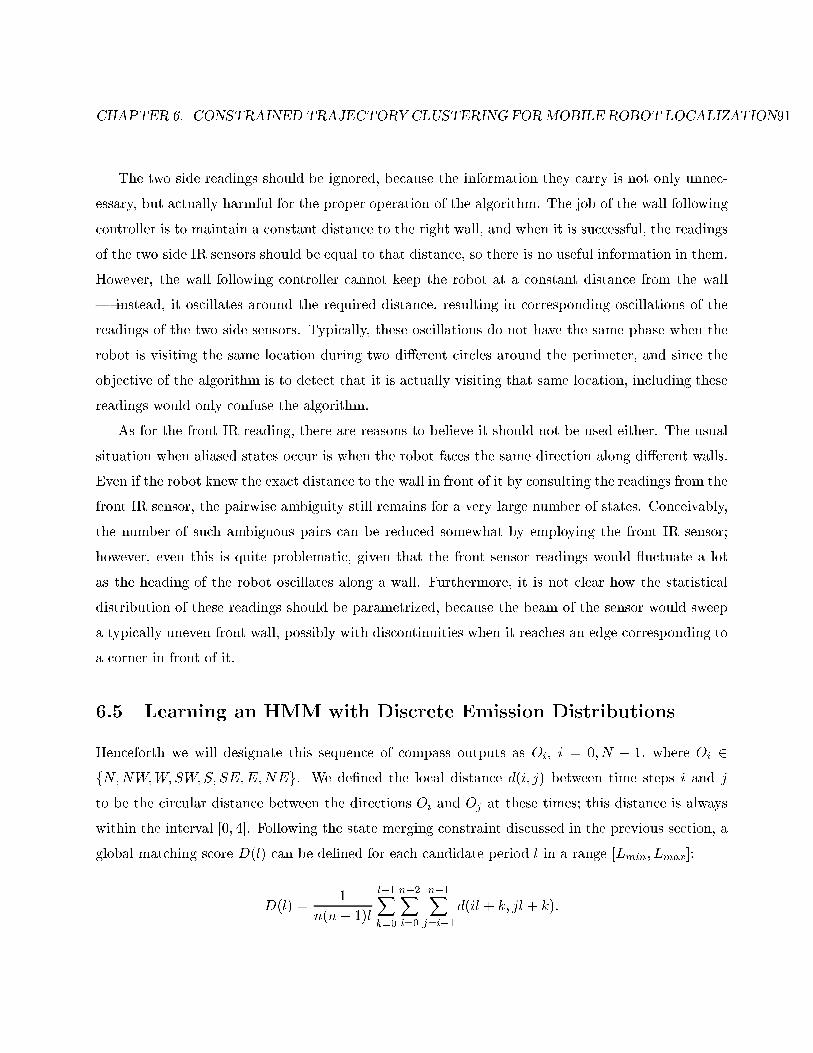
CHAPTER 6. CONSTRAINED TRAJECTORYCLUSTERING FORMOBILE ROBOT LOCALIZATION91
The two side readings should be ignored, because the information they carry is not only unnec-
essary, but actually harmful for the proper operation of the algorithm. The job of the wall following
controller is to maintain a constant distance to the right wall, and when it is successful, the readings
of the two side IR sensors should be equal to that distance, so there is no useful information in them.
However, the wall following controller cannot keep the robot at a constant distance from the wall
| instead, it oscillates around the required distance, resulting in corresponding oscillations of the
readings of the two side sensors. Typically, these oscillations do not have the same phase when the
robot is visiting the same location during two di�erent circles around the perimeter, and since the
objective of the algorithm is to detect that it is actually visiting that same location, including these
readings would only confuse the algorithm.
As for the front IR reading, there are reasons to believe it should not be used either. The usual
situation when aliased states occur is when the robot faces the same direction along di�erent walls.
Even if the robot knew the exact distance to the wall in front of it by consulting the readings from the
front IR sensor, the pairwise ambiguity still remains for a very large number of states. Conceivably,
the number of such ambiguous pairs can be reduced somewhat by employing the front IR sensor;
however, even this is quite problematic, given that the front sensor readings would uctuate a lot
as the heading of the robot oscillates along a wall. Furthermore, it is not clear how the statistical
distribution of these readings should be parametrized, because the beam of the sensor would sweep
a typically uneven front wall, possibly with discontinuities when it reaches an edge corresponding to
a corner in front of it.
6.5 Learning an HMM with Discrete Emission Distributions
Henceforth we will designate this sequence of compass outputs as Oi, i = 0; N � 1, where Oi 2
fN;NW;W;SW;S; SE;E;NEg. We de�ned the local distance d(i; j) between time steps i and j
to be the circular distance between the directions Oi and Oj at these times; this distance is always
within the interval [0; 4]. Following the state merging constraint discussed in the previous section, a
global matching score D(l) can be de�ned for each candidate period l in a range [Lmin; Lmax]:
D(l) =1
n(n� 1)l
l�1Xk=0
n�2Xi=0
n�1Xj=i+1
d(il + k; jl + k):
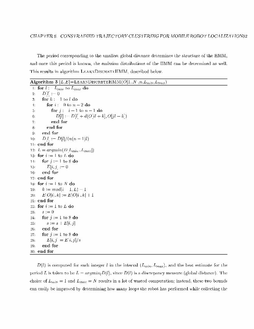
CHAPTER 6. CONSTRAINED TRAJECTORYCLUSTERING FORMOBILE ROBOT LOCALIZATION92
The period corresponding to the smallest global distance determines the structure of the HMM,
and once this period is known, the emission distributions of the HMM can be determined as well.
This results in algorithm LearnDiscreteHMM, described below.
Algorithm 3 [L,E]=LearnDiscreteHMM(O[1::N ],n,Lmin,Lmax)
1: for l := Lmin to Lmax do
2: D[l] := 03: for k := 1 to l do4: for i := 0 to n� 2 do5: for j := i+ 1 to n� 1 do6: D[l] := D[l] + d(O[il + k]; O[jl + k])7: end for
8: end for
9: end for
10: D[l] := D[l]=(n(n� 1)l)11: end for
12: L = argmin(D[Lmin::Lmax])13: for i := 1 to L do
14: for j := 1 to 8 do15: E[i; j] := 016: end for
17: end for
18: for i := 1 to N do
19: k := mod(i� 1; L) + 120: E[O[i]; k] := E[O[i]; k] + 121: end for
22: for i := 1 to L do
23: s := 024: for j := 1 to 8 do25: s := s+E[i; j]26: end for
27: for j := 1 to 8 do28: E[i; j] = E[i; j]=s29: end for
30: end for
D(l) is computed for each integer l in the interval (Lmin; Lmax), and the best estimate for the
period L is taken to be L = argminlD(l), since D(l) is a discrepancy measure (global distance). The
choice of Lmin = 1 and Lmax = N results in a lot of wasted computation; instead, these two bounds
can easily be improved by determining how many loops the robot has performed while collecting the
CHAPTER 6. CONSTRAINED TRAJECTORYCLUSTERING FORMOBILE ROBOT LOCALIZATION93
observation data. To this end, we set a counter C = 0 at the start of the sequence and increment
it by one each time the compass reading changes counter-clockwise (e.g. from north to northwest),
and decrement it by one if the reading changes clockwise (e.g., from south to southwest). When
there is no change in compass direction, the counter remains unchanged too. After all N readings in
the sequence have been processed, the integer part n of the ratio C=8 is a reliable estimate of how
many complete loops the robot circled. Hence, the limits can be modi�ed as Lmin = N=(n+ 1) and
Lmax = N=n. Note, however, that attempting to �nd the period itself as 8N=C results in a very
imprecise estimate, and leads to the creation of unusable HMMs.
When the algorithm �nds out by comparing trajectories that the system must have visited the
same state (position) at two di�erent moments in time, it establishes an equivalence class between
these two moments. By �nding the correct disjoint equivalence classes for each moment in time, the
algorithm in e�ect introduces a set of states for the HMM and determines the sequence of states
visited for each time step of the sequence by labeling it with its equivalence class.
Once it has been determined which state of the HMM was visited at each step in time, computing
the probabilities in the transition and emission tables of the HMM is trivial and reduces to counting
frequencies of occurrence, because at this point there are no more hidden variables in the model. Cer-
tainly, any errors in labeling hidden states would transfer into errors in those probability estimates,
which makes the problem of correctly merging states of primary importance in our method.
It should be noted that the compass is used primarily as a highly repeatable sensor, and not as
an indicator of the true heading of the robot. The type of compass we are using is often dismissed as
unreliable, because it is strongly in uenced by local variations in magnetic �eld. While this is true, it
has no e�ect on our algorithm, which could use any sensor that is highly repeatable. No matter how
much the local magnetic �eld is distorted by metal objects standing nearby, that �eld is stationary
and provides perfect repeatability of readings. Of course, this sensor is also very ambiguous | on
the average one eighth of all locations would produce the same reading | but this is not an obstacle
to our algorithm, which analyzes whole sequences of percepts to disambiguate states.
6.6 Experimental Environment and Results
We tested the algorithm from the previous section in the experimental world shown in Fig. 6.3,
which consisted of walls in a regular oÆce-building corridor and pieces of cardboard to close o� the

CHAPTER 6. CONSTRAINED TRAJECTORYCLUSTERING FORMOBILE ROBOT LOCALIZATION94
contour. The control loop and data trace acquisition part of the algorithm were implemented in C++
under PalmOS and ran on the robot, while the algorithm for building the HMM was implemented
in Matlab on a UNIX workstation, due to the low speed of the CPU on-board the robot (16MHz).
Figure 6.3: Experimental world for Mr. Spoon. Approximate sizes are 5m by 5m. The initiallocation of the robot is shown along with its direction of motion.
An observation trace of 2; 000 time points was collected while the robot was following the contour
of the environment by means of the wall-following controller described above, parametrized as shown
in the �rst column of Table 6.1. (Since the translational velocity was v = 9cm=sec and the control
period was 290ms, an observation was taken approximately every 3cm along the perimeter.) These
data were split into a training set (N = 1; 500 data points), and testing set (500) points. The points
in the training set were used by our algorithm to build an HMM, and the sequence in the testing
set was used to evaluate the ability of the robot to localize itself and track its state by means of the
learned HMM. The training data are shown in Fig. 6.4.
The cumulative number of direction changes over the 1; 500 training steps was found to be
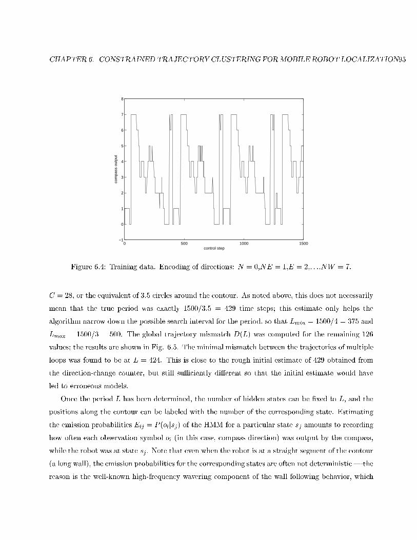
CHAPTER 6. CONSTRAINED TRAJECTORYCLUSTERING FORMOBILE ROBOT LOCALIZATION95
0 500 1000 1500−1
0
1
2
3
4
5
6
7
8
control step
com
pass
out
put
Figure 6.4: Training data. Encoding of directions: N = 0,NE = 1,E = 2,: : :,NW = 7.
C = 28, or the equivalent of 3:5 circles around the contour. As noted above, this does not necessarily
mean that the true period was exactly 1500=3:5 = 429 time steps; this estimate only helps the
algorithm narrow down the possible search interval for the period, so that Lmin = 1500=4 = 375 and
Lmax = 1500=3 = 500. The global trajectory mismatch D(L) was computed for the remaining 126
values; the results are shown in Fig. 6.5. The minimal mismatch between the trajectories of multiple
loops was found to be at L = 424. This is close to the rough initial estimate of 429 obtained from
the direction-change counter, but still suÆciently di�erent so that the initial estimate would have
led to erroneous models.
Once the period L has been determined, the number of hidden states can be �xed to L, and the
positions along the contour can be labeled with the number of the corresponding state. Estimating
the emission probabilities Eij = P (oijsj) of the HMM for a particular state sj amounts to recording
how often each observation symbol oi (in this case, compass direction) was output by the compass,
while the robot was at state sj. Note that even when the robot is at a straight segment of the contour
(a long wall), the emission probabilities for the corresponding states are often not deterministic | the
reason is the well-known high-frequency wavering component of the wall following behavior, which
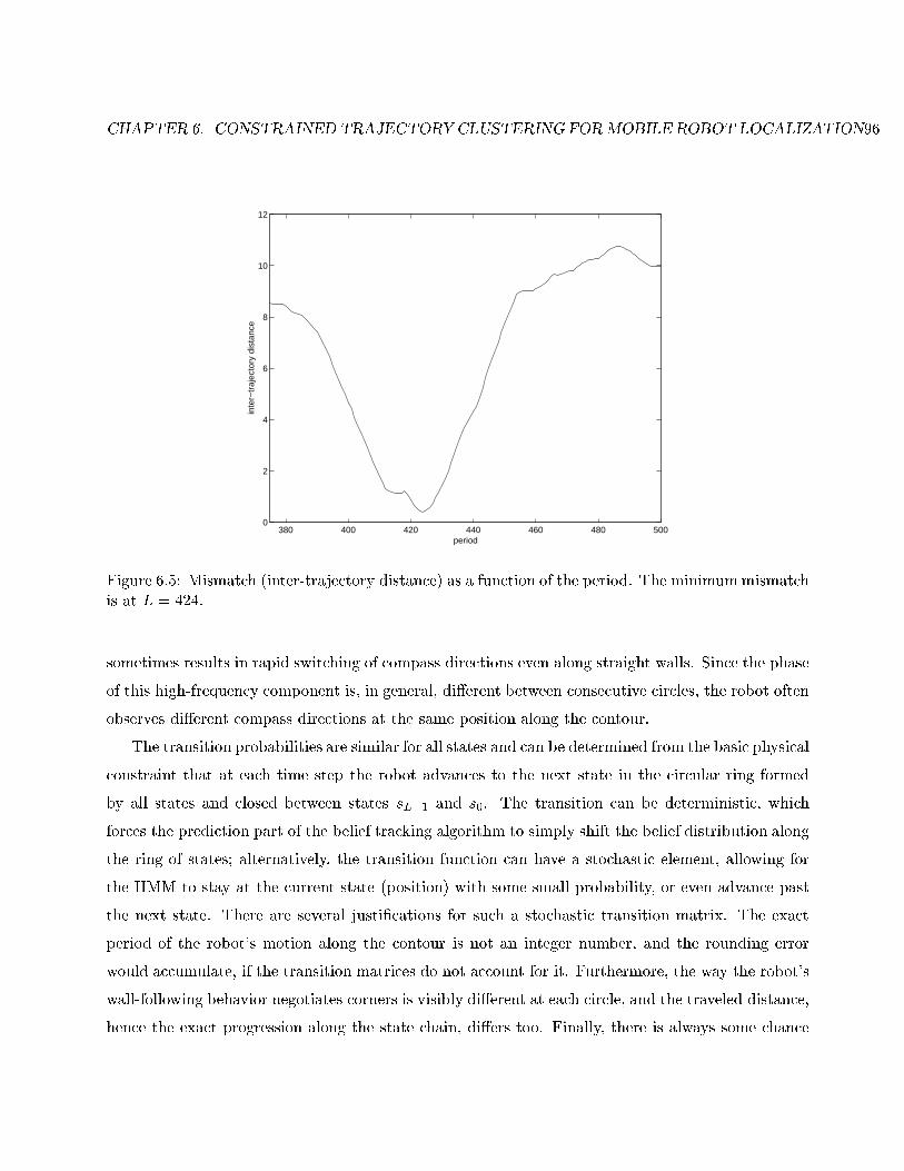
CHAPTER 6. CONSTRAINED TRAJECTORYCLUSTERING FORMOBILE ROBOT LOCALIZATION96
380 400 420 440 460 480 5000
2
4
6
8
10
12
period
inte
r−tr
ajec
tory
dis
tanc
e
Figure 6.5: Mismatch (inter-trajectory distance) as a function of the period. The minimummismatchis at L = 424.
sometimes results in rapid switching of compass directions even along straight walls. Since the phase
of this high-frequency component is, in general, di�erent between consecutive circles, the robot often
observes di�erent compass directions at the same position along the contour.
The transition probabilities are similar for all states and can be determined from the basic physical
constraint that at each time step the robot advances to the next state in the circular ring formed
by all states and closed between states sL�1 and s0. The transition can be deterministic, which
forces the prediction part of the belief tracking algorithm to simply shift the belief distribution along
the ring of states; alternatively, the transition function can have a stochastic element, allowing for
the HMM to stay at the current state (position) with some small probability, or even advance past
the next state. There are several justi�cations for such a stochastic transition matrix. The exact
period of the robot's motion along the contour is not an integer number, and the rounding error
would accumulate, if the transition matrices do not account for it. Furthermore, the way the robot's
wall-following behavior negotiates corners is visibly di�erent at each circle, and the traveled distance,
hence the exact progression along the state chain, di�ers too. Finally, there is always some chance
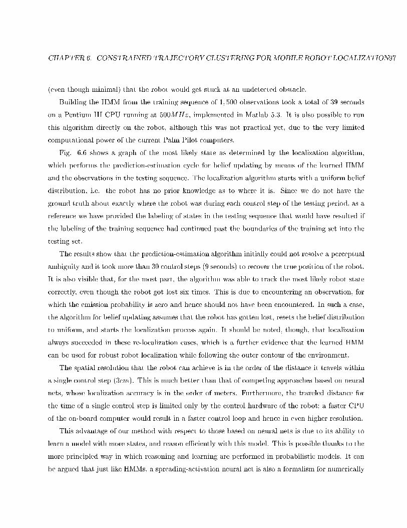
CHAPTER 6. CONSTRAINED TRAJECTORYCLUSTERING FORMOBILE ROBOT LOCALIZATION97
(even though minimal) that the robot would get stuck at an undetected obstacle.
Building the HMM from the training sequence of 1; 500 observations took a total of 39 seconds
on a Pentium III CPU running at 500MHz, implemented in Matlab 5.3. It is also possible to run
this algorithm directly on the robot, although this was not practical yet, due to the very limited
computational power of the current Palm Pilot computers.
Fig. 6.6 shows a graph of the most likely state as determined by the localization algorithm,
which performs the prediction-estimation cycle for belief updating by means of the learned HMM
and the observations in the testing sequence. The localization algorithm starts with a uniform belief
distribution, i.e. the robot has no prior knowledge as to where it is. Since we do not have the
ground truth about exactly where the robot was during each control step of the testing period, as a
reference we have provided the labeling of states in the testing sequence that would have resulted if
the labeling of the training sequence had continued past the boundaries of the training set into the
testing set.
The results show that the prediction-estimation algorithm initially could not resolve a perceptual
ambiguity and it took more than 30 control steps (9 seconds) to recover the true position of the robot.
It is also visible that, for the most part, the algorithm was able to track the most-likely robot state
correctly, even though the robot got lost six times. This is due to encountering an observation, for
which the emission probability is zero and hence should not have been encountered. In such a case,
the algorithm for belief updating assumes that the robot has gotten lost, resets the belief distribution
to uniform, and starts the localization process again. It should be noted, though, that localization
always succeeded in these re-localization cases, which is a further evidence that the learned HMM
can be used for robust robot localization while following the outer contour of the environment.
The spatial resolution that the robot can achieve is in the order of the distance it travels within
a single control step (3cm). This is much better than that of competing approaches based on neural
nets, whose localization accuracy is in the order of meters. Furthermore, the traveled distance for
the time of a single control step is limited only by the control hardware of the robot; a faster CPU
of the on-board computer would result in a faster control loop and hence in even higher resolution.
This advantage of our method with respect to those based on neural nets is due to its ability to
learn a model with more states, and reason eÆciently with this model. This is possible thanks to the
more principled way in which reasoning and learning are performed in probabilistic models. It can
be argued that just like HMMs, a spreading-activation neural net is also a formalism for numerically
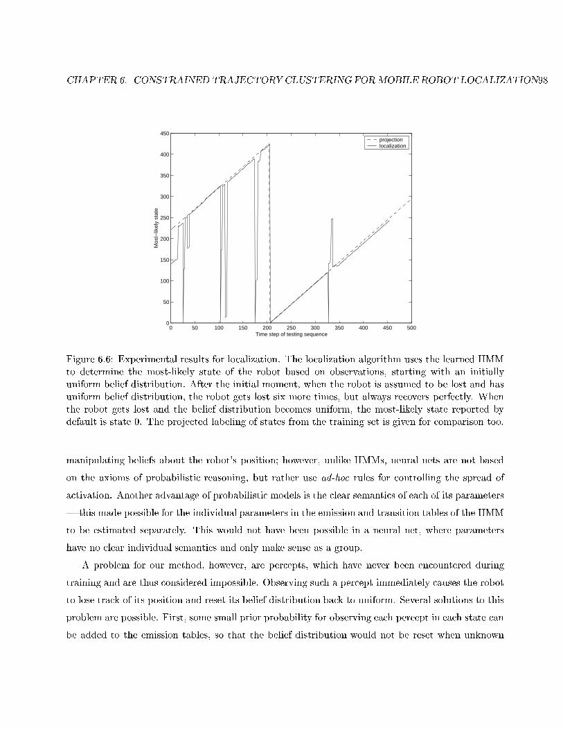
CHAPTER 6. CONSTRAINED TRAJECTORYCLUSTERING FORMOBILE ROBOT LOCALIZATION98
0 50 100 150 200 250 300 350 400 450 5000
50
100
150
200
250
300
350
400
450
Time step of testing sequence
Mos
t−lik
ely
stat
e
projection localization
Figure 6.6: Experimental results for localization. The localization algorithm uses the learned HMMto determine the most-likely state of the robot based on observations, starting with an initiallyuniform belief distribution. After the initial moment, when the robot is assumed to be lost and hasuniform belief distribution, the robot gets lost six more times, but always recovers perfectly. Whenthe robot gets lost and the belief distribution becomes uniform, the most-likely state reported bydefault is state 0. The projected labeling of states from the training set is given for comparison too.
manipulating beliefs about the robot's position; however, unlike HMMs, neural nets are not based
on the axioms of probabilistic reasoning, but rather use ad-hoc rules for controlling the spread of
activation. Another advantage of probabilistic models is the clear semantics of each of its parameters
| this made possible for the individual parameters in the emission and transition tables of the HMM
to be estimated separately. This would not have been possible in a neural net, where parameters
have no clear individual semantics and only make sense as a group.
A problem for our method, however, are percepts, which have never been encountered during
training and are thus considered impossible. Observing such a percept immediately causes the robot
to lose track of its position and reset its belief distribution back to uniform. Several solutions to this
problem are possible. First, some small prior probability for observing each percept in each state can
be added to the emission tables, so that the belief distribution would not be reset when unknown
CHAPTER 6. CONSTRAINED TRAJECTORYCLUSTERING FORMOBILE ROBOT LOCALIZATION99
percepts are seen. Second, the eight compass directions can be modeled not as independent discrete
symbols, but as continuous values, and the distance between these values can be exploited while
learning the HMM: for example, if the compass direction north has been observed in a particular
state, the probability of also observing northwest and northeast in that state could increase too.
Furthermore, the probability that south will be observed at this state should decrease, because south
is farthest away from north. One implementation of this possibility is explored in the next section.
6.7 Learning an HMM with Circular Emission Distributions
The method for learning an HMM of the contour described in the previous section assumed that the
compass output was a discrete nominal variable with eight unrelated values. However, in reality, the
direction returned by the compass is a naturally continuous variable which has been discretized in-
ternally by the compass. Hence, the emission distribution of the HMM at each state could be learned
by estimating the parameters of a continuous circular distribution for each state, and discretizing it
into eight bins corresponding to the eight discrete readings provided by the compass.
Circular distributions and their associated directional statistics have been used in many areas of
science where angular random variables appear (Mardia & Jupp, 2000). Most non-directional (linear)
distributions have their directional counterparts, and there is a choice of directional distributions for
the compass output variable we are trying to model. Such a distribution should re ect the fact that
when the robot is at a particular location, there is a single preferred compass heading corresponding
to the local magnetic �eld, i.e., the distribution should be unimodal. Furthermore, such a distribution
should re ect the possible deviations in compass direction resulting from uctuations in the magnetic
�eld, as well as the wavering behavior of the wall following controller. As a result of this behavior,
the heading of the robot at the same location, but on two di�erent circles around the perimeter,
would typically vary signi�cantly.
Hence, the type of distribution that could model the compass output should resemble the Gaussian
distribution | it should be centered around a preferred direction (similar to mean), and should also
have a spread parameter (similar to variance). Unlike the Gaussian distribution, however, it should
be circular, i.e. its probability density function (pdf) f should obey the property f(x) = f(2� + x),
for any angle x.
Several circular counterparts to the Gaussian distribution have been used, among which the
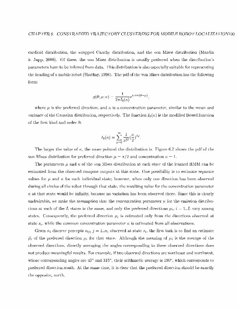
CHAPTER 6. CONSTRAINED TRAJECTORYCLUSTERING FORMOBILE ROBOT LOCALIZATION100
cardioid distribution, the wrapped Cauchy distribution, and the von Mises distribution (Mardia
& Jupp, 2000). Of these, the von Mises distribution is usually preferred when the distribution's
parameters have to be inferred from data. This distribution is also especially suitable for representing
the heading of a mobile robot (Shatkay, 1998). The pdf of the von Mises distribution has the following
form:
g(�;�;�) =1
2�I0(�)e� cos(���);
where � is the preferred direction, and � is a concentration parameter, similar to the mean and
variance of the Gaussian distribution, respectively. The function I0(�) is the modi�ed Bessel function
of the �rst kind and order 0:
I0(�) =1Xx=0
1
x!2(�
2)2x:
The larger the value of �, the more pointed the distribution is. Figure 6.7 shows the pdf of the
von Mises distribution for preferred direction � = �=2 and concentration � = 1.
The parameters � and � of the von Mises distribution at each state of the learned HMM can be
estimated from the observed compass outputs at this state. One possibility is to estimate separate
values for � and � for each individual state; however, when only one direction has been observed
during all circles of the robot through that state, the resulting value for the concentration parameter
� at that state would be in�nity, because no variation has been observed there. Since this is clearly
undesirable, we make the assumption that the concentration parameter � for the emission distribu-
tions at each of the L states is the same, and only the preferred directions �i, i = 1::L vary among
states. Consequently, the preferred direction �i is estimated only from the directions observed at
state si, while the common concentration parameter � is estimated from all observations.
Given ni discrete percepts oij , j = 1::ni observed at state si, the �rst task is to �nd an estimate
��i of the preferred direction �i for that state. Although the meaning of �i is the average of the
observed directions, directly averaging the angles corresponding to these observed directions does
not produce meaningful results. For example, if two observed directions are northeast and northwest,
whose corresponding angles are 45o and 315o, their arithmetic average is 180o, which corresponds to
preferred direction south. At the same time, it is clear that the preferred direction should be exactly
the opposite, north.
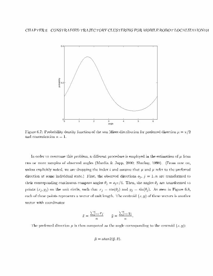
CHAPTER 6. CONSTRAINED TRAJECTORYCLUSTERING FORMOBILE ROBOT LOCALIZATION101
0 1 2 3 4 5 60
0.2
0.4
angle
prob
abili
ty
Figure 6.7: Probability density function of the von Mises distribution for preferred direction � = �=2and concentration � = 1.
In order to overcome this problem, a di�erent procedure is employed in the estimation of � from
two or more samples of observed angles (Mardia & Jupp, 2000; Shatkay, 1998). (From now on,
unless explicitly noted, we are dropping the index i and assume that � and �� refer to the preferred
direction at some individual state.) First, the observed directions oj , j = 1::n are transformed to
their corresponding continuous compass angles �j = oj�=4. Then, the angles �j are transformed to
points (xj; yj) on the unit circle, such that xj = cos(�j) and yj = sin(�j). As seen in Figure 6.8,
each of these points represents a vector of unit length. The centroid (�x; �y) of these vectors is another
vector with coordinates:
�x =
Pnj=1 xj
n�y =
Pnj=1 yj
n:
The preferred direction �� is then computed as the angle corresponding to the centroid (�x; �y):
�� = atan2(�y; �x):
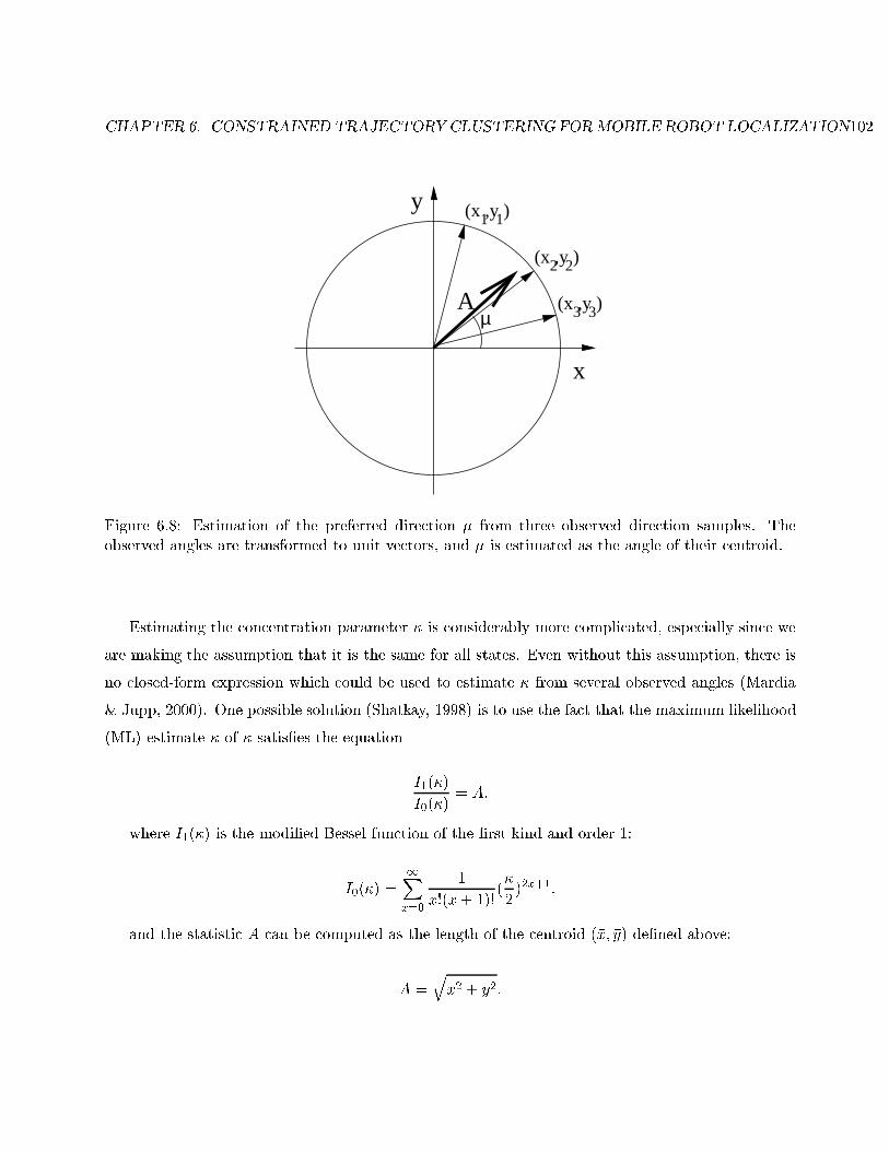
CHAPTER 6. CONSTRAINED TRAJECTORYCLUSTERING FORMOBILE ROBOT LOCALIZATION102
y
x
Aµ
(x ,y )
(x ,y )
(x ,y )
1 1
2 2
3 3
Figure 6.8: Estimation of the preferred direction � from three observed direction samples. Theobserved angles are transformed to unit vectors, and � is estimated as the angle of their centroid.
Estimating the concentration parameter � is considerably more complicated, especially since we
are making the assumption that it is the same for all states. Even without this assumption, there is
no closed-form expression which could be used to estimate � from several observed angles (Mardia
& Jupp, 2000). One possible solution (Shatkay, 1998) is to use the fact that the maximum likelihood
(ML) estimate �� of � satis�es the equation
I1(�)
I0(�)= A;
where I1(�) is the modi�ed Bessel function of the �rst kind and order 1:
I0(�) =1Xx=0
1
x!(x+ 1)!(�
2)2x+1;
and the statistic A can be computed as the length of the centroid (�x; �y) de�ned above:
A =q�x2 + �y2:
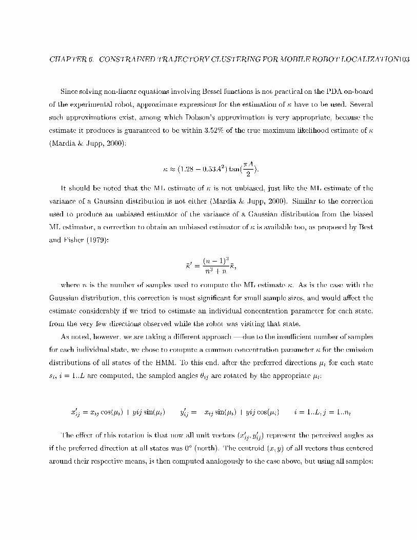
CHAPTER 6. CONSTRAINED TRAJECTORYCLUSTERING FORMOBILE ROBOT LOCALIZATION103
Since solving non-linear equations involving Bessel functions is not practical on the PDA on-board
of the experimental robot, approximate expressions for the estimation of � have to be used. Several
such approximations exist, among which Dobson's approximation is very appropriate, because the
estimate it produces is guaranteed to be within 3:52% of the true maximum likelihood estimate of �
(Mardia & Jupp, 2000):
�� � (1:28 � 0:53A2) tan(�A
2):
It should be noted that the ML estimate of � is not unbiased, just like the ML estimate of the
variance of a Gaussian distribution is not either (Mardia & Jupp, 2000). Similar to the correction
used to produce an unbiased estimator of the variance of a Gaussian distribution from the biased
ML estimator, a correction to obtain an unbiased estimator of � is available too, as proposed by Best
and Fisher (1979):
��0 =(n� 1)3
n3 + n��;
where n is the number of samples used to compute the ML estimate ��. As is the case with the
Gaussian distribution, this correction is most signi�cant for small sample sizes, and would a�ect the
estimate considerably if we tried to estimate an individual concentration parameter for each state,
from the very few directions observed while the robot was visiting that state.
As noted, however, we are taking a di�erent approach | due to the insuÆcient number of samples
for each individual state, we chose to compute a common concentration parameter �� for the emission
distributions of all states of the HMM. To this end, after the preferred directions �i for each state
si, i = 1::L are computed, the sampled angles �ij are rotated by the appropriate �i:
x0ij = xij cos(�i) + yij sin(�i) y0ij = �xij sin(�i) + yij cos(�i) i = 1::L; j = 1::ni
The e�ect of this rotation is that now all unit vectors (x0ij ; y0ij) represent the perceived angles as
if the preferred direction at all states was 0o (north). The centroid (�x; �y) of all vectors thus centered
around their respective means, is then computed analogously to the case above, but using all samples:
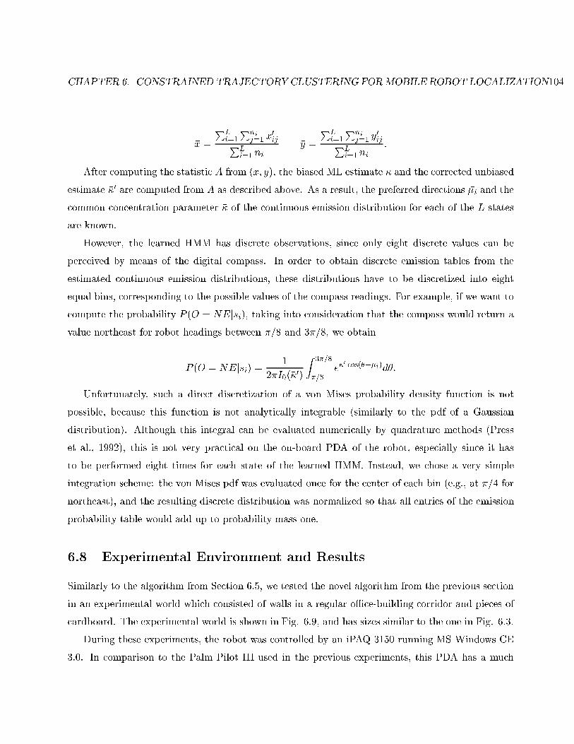
CHAPTER 6. CONSTRAINED TRAJECTORYCLUSTERING FORMOBILE ROBOT LOCALIZATION104
�x =
PLi=1
Pni
j=1 x0ijPL
i=1 ni�y =
PLi=1
Pni
j=1 y0ijPL
i=1 ni:
After computing the statistic A from (�x; �y), the biased ML estimate �� and the corrected unbiased
estimate ��0 are computed from A as described above. As a result, the preferred directions ��i and the
common concentration parameter �� of the continuous emission distribution for each of the L states
are known.
However, the learned HMM has discrete observations, since only eight discrete values can be
perceived by means of the digital compass. In order to obtain discrete emission tables from the
estimated continuous emission distributions, these distributions have to be discretized into eight
equal bins, corresponding to the possible values of the compass readings. For example, if we want to
compute the probability P (O = NEjsi), taking into consideration that the compass would return a
value northeast for robot headings between �=8 and 3�=8, we obtain
P (O = NEjsi) =1
2�I0(��0)
Z 3�=8
�=8e��
0 cos(�� ��i)d�:
Unfortunately, such a direct discretization of a von Mises probability density function is not
possible, because this function is not analytically integrable (similarly to the pdf of a Gaussian
distribution). Although this integral can be evaluated numerically by quadrature methods (Press
et al., 1992), this is not very practical on the on-board PDA of the robot, especially since it has
to be performed eight times for each state of the learned HMM. Instead, we chose a very simple
integration scheme: the von Mises pdf was evaluated once for the center of each bin (e.g., at �=4 for
northeast), and the resulting discrete distribution was normalized so that all entries of the emission
probability table would add up to probability mass one.
6.8 Experimental Environment and Results
Similarly to the algorithm from Section 6.5, we tested the novel algorithm from the previous section
in an experimental world which consisted of walls in a regular oÆce-building corridor and pieces of
cardboard. The experimental world is shown in Fig. 6.9, and has sizes similar to the one in Fig. 6.3.
During these experiments, the robot was controlled by an iPAQ 3150 running MS Windows CE
3.0. In comparison to the Palm Pilot III used in the previous experiments, this PDA has a much
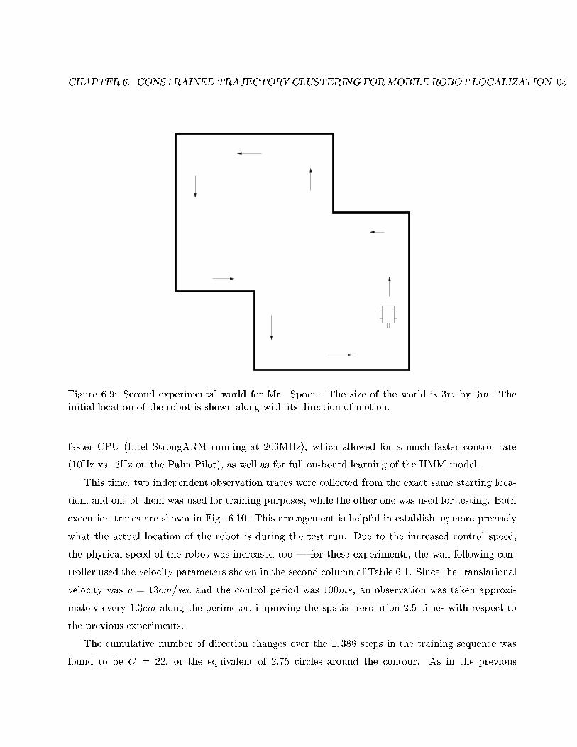
CHAPTER 6. CONSTRAINED TRAJECTORYCLUSTERING FORMOBILE ROBOT LOCALIZATION105
Figure 6.9: Second experimental world for Mr. Spoon. The size of the world is 3m by 3m. Theinitial location of the robot is shown along with its direction of motion.
faster CPU (Intel StrongARM running at 206MHz), which allowed for a much faster control rate
(10Hz vs. 3Hz on the Palm Pilot), as well as for full on-board learning of the HMM model.
This time, two independent observation traces were collected from the exact same starting loca-
tion, and one of them was used for training purposes, while the other one was used for testing. Both
execution traces are shown in Fig. 6.10. This arrangement is helpful in establishing more precisely
what the actual location of the robot is during the test run. Due to the increased control speed,
the physical speed of the robot was increased too | for these experiments, the wall-following con-
troller used the velocity parameters shown in the second column of Table 6.1. Since the translational
velocity was v = 13cm=sec and the control period was 100ms, an observation was taken approxi-
mately every 1:3cm along the perimeter, improving the spatial resolution 2:5 times with respect to
the previous experiments.
The cumulative number of direction changes over the 1; 388 steps in the training sequence was
found to be C = 22, or the equivalent of 2:75 circles around the contour. As in the previous
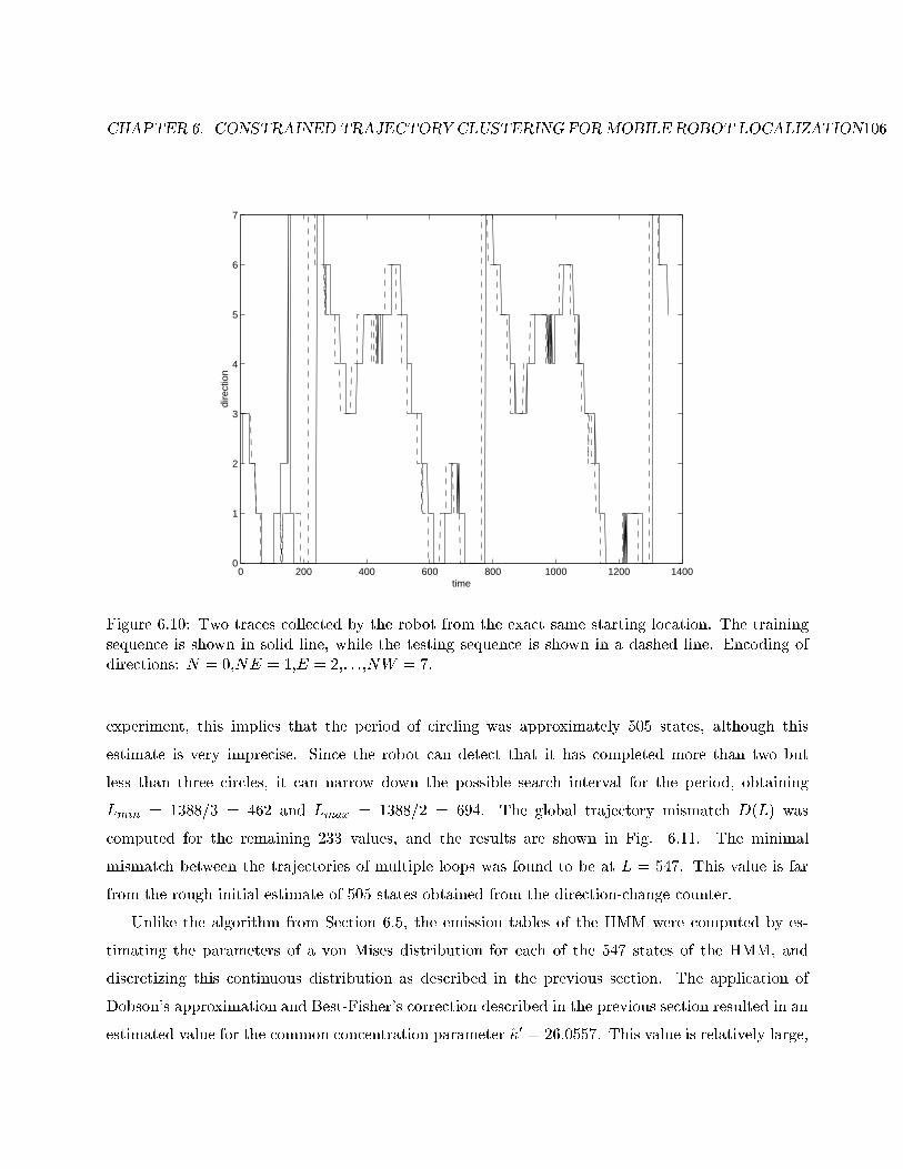
CHAPTER 6. CONSTRAINED TRAJECTORYCLUSTERING FORMOBILE ROBOT LOCALIZATION106
0 200 400 600 800 1000 1200 14000
1
2
3
4
5
6
7
time
dire
ctio
n
Figure 6.10: Two traces collected by the robot from the exact same starting location. The trainingsequence is shown in solid line, while the testing sequence is shown in a dashed line. Encoding ofdirections: N = 0,NE = 1,E = 2,: : :,NW = 7.
experiment, this implies that the period of circling was approximately 505 states, although this
estimate is very imprecise. Since the robot can detect that it has completed more than two but
less than three circles, it can narrow down the possible search interval for the period, obtaining
Lmin = 1388=3 = 462 and Lmax = 1388=2 = 694. The global trajectory mismatch D(L) was
computed for the remaining 233 values, and the results are shown in Fig. 6.11. The minimal
mismatch between the trajectories of multiple loops was found to be at L = 547. This value is far
from the rough initial estimate of 505 states obtained from the direction-change counter.
Unlike the algorithm from Section 6.5, the emission tables of the HMM were computed by es-
timating the parameters of a von Mises distribution for each of the 547 states of the HMM, and
discretizing this continuous distribution as described in the previous section. The application of
Dobson's approximation and Best-Fisher's correction described in the previous section resulted in an
estimated value for the common concentration parameter �0 = 26:0557. This value is relatively large,
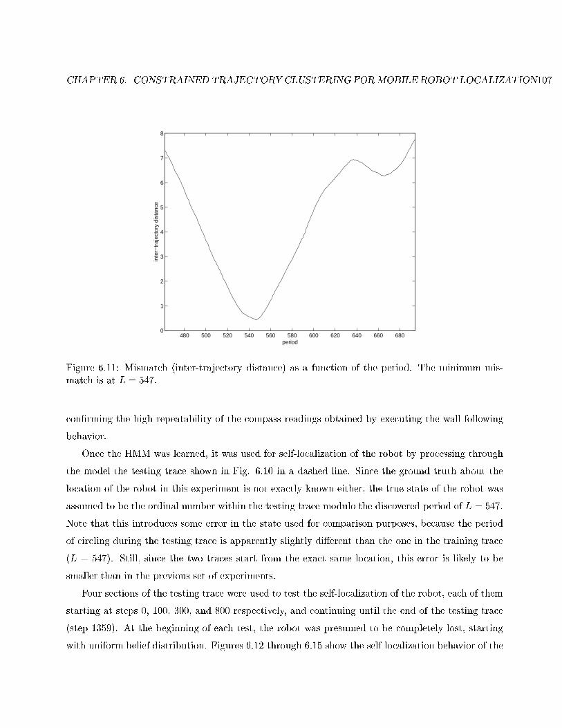
CHAPTER 6. CONSTRAINED TRAJECTORYCLUSTERING FORMOBILE ROBOT LOCALIZATION107
480 500 520 540 560 580 600 620 640 660 6800
1
2
3
4
5
6
7
8
period
inte
r−tr
ajec
tory
dis
tanc
e
Figure 6.11: Mismatch (inter-trajectory distance) as a function of the period. The minimum mis-match is at L = 547.
con�rming the high repeatability of the compass readings obtained by executing the wall-following
behavior.
Once the HMM was learned, it was used for self-localization of the robot by processing through
the model the testing trace shown in Fig. 6.10 in a dashed line. Since the ground truth about the
location of the robot in this experiment is not exactly known either, the true state of the robot was
assumed to be the ordinal number within the testing trace modulo the discovered period of L = 547.
Note that this introduces some error in the state used for comparison purposes, because the period
of circling during the testing trace is apparently slightly di�erent than the one in the training trace
(L = 547). Still, since the two traces start from the exact same location, this error is likely to be
smaller than in the previous set of experiments.
Four sections of the testing trace were used to test the self-localization of the robot, each of them
starting at steps 0, 100, 300, and 800 respectively, and continuing until the end of the testing trace
(step 1359). At the beginning of each test, the robot was presumed to be completely lost, starting
with uniform belief distribution. Figures 6.12 through 6.15 show the self-localization behavior of the
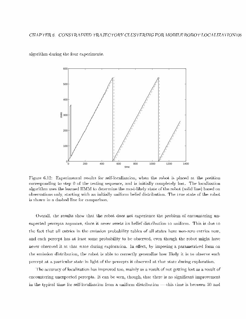
CHAPTER 6. CONSTRAINED TRAJECTORYCLUSTERING FORMOBILE ROBOT LOCALIZATION108
algorithm during the four experiments.
0 200 400 600 800 1000 1200 14000
100
200
300
400
500
600
time
stat
e
Figure 6.12: Experimental results for self-localization, when the robot is placed at the positioncorresponding to step 0 of the testing sequence, and is initially completely lost. The localizationalgorithm uses the learned HMM to determine the most-likely state of the robot (solid line) based onobservations only, starting with an initially uniform belief distribution. The true state of the robotis shown in a dashed line for comparison.
Overall, the results show that the robot does not experience the problem of encountering un-
expected percepts anymore, since it never resets its belief distribution to uniform. This is due to
the fact that all entries in the emission probability tables of all states have non-zero entries now,
and each percept has at least some probability to be observed, even though the robot might have
never observed it at that state during exploration. In e�ect, by imposing a parametrized form on
the emission distribution, the robot is able to correctly generalize how likely it is to observe each
percept at a particular state in light of the percepts it observed at that state during exploration.
The accuracy of localization has improved too, mainly as a result of not getting lost as a result of
encountering unexpected percepts. It can be seen, though, that there is no signi�cant improvement
in the typical time for self-localization from a uniform distribution | this time is between 50 and
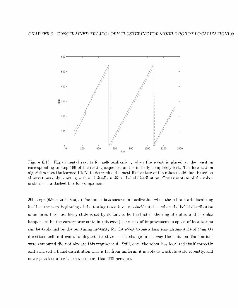
CHAPTER 6. CONSTRAINED TRAJECTORYCLUSTERING FORMOBILE ROBOT LOCALIZATION109
0 200 400 600 800 1000 1200 14000
100
200
300
400
500
600
time
stat
e
Figure 6.13: Experimental results for self-localization, when the robot is placed at the positioncorresponding to step 100 of the testing sequence, and is initially completely lost. The localizationalgorithm uses the learned HMM to determine the most-likely state of the robot (solid line) based onobservations only, starting with an initially uniform belief distribution. The true state of the robotis shown in a dashed line for comparison.
200 steps (65cm to 260cm). (The immediate success in localization when the robot starts localizing
itself at the very beginning of the testing trace is only coincidental | when the belief distribution
is uniform, the most likely state is set by default to be the �rst in the ring of states, and this also
happens to be the correct true state in this case.) The lack of improvement in speed of localization
can be explained by the remaining necessity for the robot to see a long enough sequence of compass
directions before it can disambiguate its state | the change in the way the emission distributions
were computed did not obviate this requirement. Still, once the robot has localized itself correctly
and achieved a belief distribution that is far from uniform, it is able to track its state robustly, and
never gets lost after it has seen more than 200 percepts.
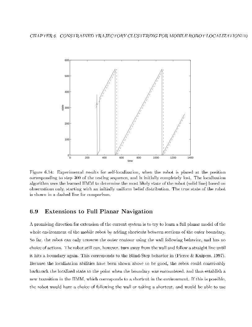
CHAPTER 6. CONSTRAINED TRAJECTORYCLUSTERING FORMOBILE ROBOT LOCALIZATION110
0 200 400 600 800 1000 1200 14000
100
200
300
400
500
600
time
stat
e
Figure 6.14: Experimental results for self-localization, when the robot is placed at the positioncorresponding to step 300 of the testing sequence, and is initially completely lost. The localizationalgorithm uses the learned HMM to determine the most-likely state of the robot (solid line) based onobservations only, starting with an initially uniform belief distribution. The true state of the robotis shown in a dashed line for comparison.
6.9 Extensions to Full Planar Navigation
A promising direction for extension of the current system is to try to learn a full planar model of the
whole environment of the mobile robot by adding shortcuts between sections of the outer boundary.
So far, the robot can only traverse the outer contour using the wall following behavior, and has no
choice of actions. The robot still can, however, turn away from the wall and follow a straight line until
it hits a boundary again. This corresponds to the Blind-Step behavior in (Pierce & Kuipers, 1997).
Because the localization abilities have been shown above to be good, the robot could conceivably
backtrack the localized state to the point when the boundary was encountered, and thus establish a
new transition in the HMM, which corresponds to a shortcut in the environment. If this is possible,
the robot would have a choice of following the wall or taking a shortcut, and would be able to use
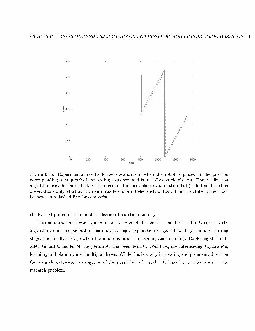
CHAPTER 6. CONSTRAINED TRAJECTORYCLUSTERING FORMOBILE ROBOT LOCALIZATION111
0 200 400 600 800 1000 1200 14000
100
200
300
400
500
600
time
stat
e
Figure 6.15: Experimental results for self-localization, when the robot is placed at the positioncorresponding to step 800 of the testing sequence, and is initially completely lost. The localizationalgorithm uses the learned HMM to determine the most-likely state of the robot (solid line) based onobservations only, starting with an initially uniform belief distribution. The true state of the robotis shown in a dashed line for comparison.
the learned probabilistic model for decision-theoretic planning.
This modi�cation, however, is outside the scope of this thesis | as discussed in Chapter 1, the
algorithms under consideration here have a single exploration stage, followed by a model-learning
stage, and �nally a stage when the model is used in reasoning and planning. Exploring shortcuts
after an initial model of the perimeter has been learned would require interleaving exploration,
learning, and planning over multiple phases. While this is a very interesting and promising direction
for research, extensive investigation of the possibilities for such interleaved operation is a separate
research problem.
Chapter 7
Learning POMDPs by Clustering
Trajectory Features
The idea of learning probabilistic models by clustering trajectories can also be applied to other
types of robotic tasks and other sensor modalities. In this chapter we consider a visual servo-control
manipulation task which is related to the Acrobot (Spong, 1995) and inverted pendulum (Jervis &
Fallside, 1992) tasks, as well as to the original centrifugal governor problem of James Watt, which
started the theoretical analysis of control systems in the 18th century.
In this chapter, we will also explore several additional questions. The �rst one is whether the
learning algorithm can perform clustering directly in the space of continuous observations, instead
of quantizing them �rst into discrete symbols. The second one is whether features from sequences of
observations can be used instead of the sequences themselves. The third one is whether the length
of considered sequences can be limited to a �xed number based on understanding of the nature of
the dynamical system to be controlled.
7.1 Experimental Manipulator and Task
For our experiments, we built an experimental robotic arm controlled by a camera, and considered
a manipulation task which requires high control rates. A hollow ball of radius 75mm is attached
to the second link of a simple 2-degrees-of-freedom (DOF) planar robot manipulator with links of
length l1 = 265mm and l2 = 115mm, respectively (Fig. 7.1). The two joints move in approximately
112
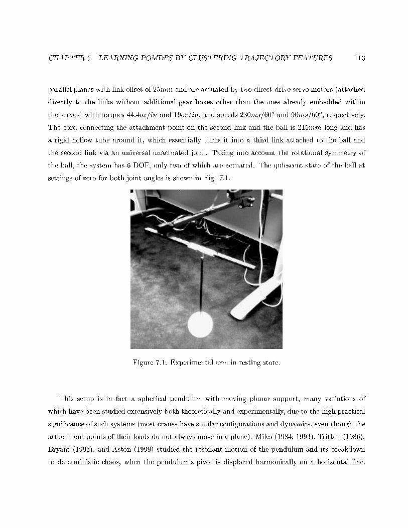
CHAPTER 7. LEARNING POMDPS BY CLUSTERING TRAJECTORY FEATURES 113
parallel planes with link o�set of 25mm and are actuated by two direct-drive servo motors (attached
directly to the links without additional gear boxes other than the ones already embedded within
the servos) with torques 44:4oz=in and 19oz=in, and speeds 230ms=60o and 90ms=60o, respectively.
The cord connecting the attachment point on the second link and the ball is 215mm long and has
a rigid hollow tube around it, which essentially turns it into a third link attached to the ball and
the second link via an universal unactuated joint. Taking into account the rotational symmetry of
the ball, the system has 6 DOF, only two of which are actuated. The quiescent state of the ball at
settings of zero for both joint angles is shown in Fig. 7.1.
Figure 7.1: Experimental arm in resting state.
This setup is in fact a spherical pendulum with moving planar support, many variations of
which have been studied extensively both theoretically and experimentally, due to the high practical
signi�cance of such systems (most cranes have similar con�gurations and dynamics, even though the
attachment points of their loads do not always move in a plane). Miles (1984; 1993), Tritton (1986),
Bryant (1993), and Aston (1999) studied the resonant motion of the pendulum and its breakdown
to deterministic chaos, when the pendulum's pivot is displaced harmonically on a horizontal line.
CHAPTER 7. LEARNING POMDPS BY CLUSTERING TRAJECTORY FEATURES 114
Heng and Martienssen (1992) explored the behavior of the system, when a harmonically modulated
torque is applied in one direction instead. Akulenko (2000b) analyzed the case when the plane of
rotation of the attachment point of the pendulum moves vertically.
Due to the rich dynamics of the system, which will be analyzed in the following section, it is not
likely that a single control method exists that can make the pendulum follow arbitrary trajectories.
Another reason such a method might not exist is the large discrepancy between total and actuated
degrees of freedom of the system. For these reasons, we chose a speci�c experimental task, which
e�ectively limits the degrees of freedom of the system.
The objective of the controller is to move the manipulator so as to keep the ball as high as possible
with minimal control e�ort. The e�ort is measured by the amount of movement of the servo-motors
per control step, which in its turn is proportional to the current and power consumed by them.
The performance of the controller is inferred from visual input. The manipulator and the ball
are observed from a Logitech QuickCam Pro camera placed 1380mm above the plane of the motion
of the attachment point of the cord to the second link, and pointed approximately perpendicular to
that plane. The camera and the servo control board are connected to a workstation. In the two sets
of experiments reported below, an image was acquired, processed, and a new control position for the
servos was determined every 90� 1:45ms (Section 7.5) and 40� 1ms (Section 7.6). (The reason for
the deviation is that the operating systems we used could only meet soft real-time constraints.) The
ball is painted in bright yellow color, and a patch of bright pink color is placed at the second link,
centered at the attachment point of the ball cord.
By tuning the color gains, exposure time, light sensitivity, brightness, and contrast of the camera,
it is possible to separate the ball and the patch from the background by thresholding the resulting
pixel intensities without any modi�cations to regular oÆce lighting conditions. Separating the ball
pixels from the patch pixels is based on color information | the red component R is larger than the
green component G for the patch pixels, and vice versa for the ball pixels. Classi�cation, though,
is not perfect: a certain number of ball pixels (usually less than 10%) are always classi�ed as patch
pixels, apparently due to the ball's specular re ection which looks red after �ltering by the camera
electronics. Experiments with classi�ers that had decision surfaces more complex than the single
line R � G = 0, including a decision tree, did not improve the classi�cation accuracy signi�cantly,
and had unacceptable running times. (The classi�er has to be applied to every pixel in the image).
Nevertheless, the centroids of the detected ball and patch pixels, even when computed with these
CHAPTER 7. LEARNING POMDPS BY CLUSTERING TRAJECTORY FEATURES 115
false-positive patch pixels, coincide fairly precisely with the attachment points of the cord to the ball
and second link, respectively, and can identify reliably the position of these points on the image plane.
The simple classi�cation rule R > G allows identi�cation of the position of the ball and attachment
point in the image plane (160 by 120 pixels) to be performed very fast (2ms on a Pentium II running
at 400MHz).
It is the Euclidean distance between these two centroids in a particular image frame that we
take as a measure of how high the ball is with respect to its resting state. The exact height is
not measurable directly, but is proportional (non-linearly) to the projection of the third link on the
image plane, so the latter is a reasonable substitute measure. When we use the word \height" in
this section and the sections on experimental results, we will mean this substitute measure.
If the measured height in an image frame t is Ht, and the applied action has cost Ct, the total
performance for that frame is Rt = Ht � �Ct, where � � 0 is a user-speci�ed multiplier expressing
the relative cost of control. The cost of applied e�ort itself is calculated as a function of the range
of motion of the arm; the two cost measures used in the two sets of experiments will be described
in Sections 7.5 and 7.6. The control objective then is to �nd a control policy �� that maximizes the
average performance of the system over an in�nite (in experiments, very large) number of control
points:
�� = argmax� limT!1
1
T
TXt=1
Ht � �Ct
Instead of building a general-purpose controller, our strategy is to force the ball into self-
stabilizing trajectories and choose the one that is optimal with respect to both height and control
e�ort. Forcing the ball to circle steadily is a suitable choice of a set of trajectories, as con�rmed from
experiments and the analysis of the system in simulation, presented in the next section. We found
that for a certain class of open-loop control schedules, the movement of the ball is self-stabilizing
around a central orbit and not too sensitive to small control delays. Such trajectories also keep the
projection of the ball quite far from the attachment point on the second link, which results in good
performance. Further analysis of the shape of these trajectories and their dependency on control
parameters is presented in the next section.
CHAPTER 7. LEARNING POMDPS BY CLUSTERING TRAJECTORY FEATURES 116
7.2 Analysis of a Harmonically Driven Spherical Pendulum
The general behavior of the arm can be studied by analyzing the equations of motion of an idealized
system, corresponding to a damped forced spherical pendulum, whose links have no mass, and all of
the mass of the ball is concentrated in a single point. This is a common idealization in physics and
control engineering.
We are interested in periodic displacements of the support of the pendulum (attachment point
of the third link to the arm via a universal unactuated joint), which would make the ball itself move
in a periodic orbit. It was established experimentally that such motions include planar circles of
the attachment point, ellipses in joint space, and rhythmical movements of the attachment points
on a single straight line. Under the last control, the ball initially starts moving in a single vertical
plane, and then quickly breaks out of that plane. It has been demonstrated that this behavior is
due to the existence of an unstable saddle point in the state space of the system (i.e., one having a
positive Lyapunov exponent in direction perpendicular to the initial plane of motion) (Miles, 1984;
Miles, 1993). Aston (1999) studied the conditions under which attractor bifurcations occur and lead
to chaotic dynamics.
Due to the large number of possible controls that �t our strategy, choosing the best one is not
a trivial problem. Furthermore, the whole set of possible driving functions that would result in
periodic behavior is not known even for the much simpler planar pendulum| as Fu�cic (1980) noted,
\the description of the set P of f , for which the equation u00+sinu = f(t) has a T -periodic solution
seems to remain a terra incognita."
Since the general approach of this thesis is to learn dynamical models which are as deterministic
as possible, choosing a driving function which might result in chaotic behavior is clearly a poor choice.
For this reason, in this section we will analyze the behavior of the system under periodic motion of
the pendulum support point with frequency ! along a circle of radius r lying in a horizontal plane.
This particular forcing mode also matches closely a peculiarity of the experimental arm | the R/C
servos attached to the links of the arm control directly the position of the end point of the arm, rather
than the more usual case when a controller regulates the torques applied to a manipulator's joints.
(In our case, position control is implemented internally to the servos by means of a fast closed-loop
controller.)
Such a movement of the support point of the pendulum imposes a rheonomic (moving) constraint
CHAPTER 7. LEARNING POMDPS BY CLUSTERING TRAJECTORY FEATURES 117
on the dynamics of the system (Sussman & Wisdom, 2001). Similarly, the third link itself imposes
the rigid-body constraint that the support point and the ball are always at a distance of l apart.
Since both of these constraints are holonomic and we are not interested in the forces which give
rise to them, we can integrate the constraints out and choose a state representation that satis�es
the constraints implicitly. Furthermore, if we assume that the rotational velocity ! is constant, we
can attach a coordinate frame to the center of the circular motion and ignore completely the �rst
two links of the manipulator, because under such motion this coordinate frame is inertial and it is
immaterial what kind of forces give rise to the rheonomic constraint. (Note, however, that this is
not the case when the arm is describing a circular motion in joint space, for example, rather than in
Cartesian space.)
When analyzing the motion of spherical pendulums, the usual approach is to express the state of
the system in terms of two angles � and � which correspond to spherical coordinates (Miles, 1984;
Akulenko, 2000a). The usual cartographic representation, where � and � correspond to latitude and
longitude, respectively, has singularities at x = y = 0, z = �l for the Cartesian coordinates (x; y; z)
of the bob of the pendulum. These singularities include the resting point x = y = 0, z = �l, which
is very undesirable, because the arm always starts at rest. Instead, the alternative parametrization
shown in Fig. 7.2 will be used, following (Aston, 1999). This choice of generalized coordinates � and
� results in the following expressions for the Cartesian coordinates of the bob of the pendulum:
x = r cos!t+ l sin � cos�
y = r sin!t+ l sin�
z = �l cos � cos�
While this representation has singularities too (at x = z = 0, y = �l), they lie outside of the
range of motion of the ball that we are considering (the ball starts hitting the �rst two links of the
arm when z = 0, so we are not interested in bringing up the ball that high).
The chosen coordinates describe exactly the degrees of freedom of the system and automati-
cally incorporate all available constraints, which makes the application of the Lagrangian approach
to deriving the equations of motion especially suitable. Lagrangian mechanics, unlike Newtonian
mechanics, can analyze the motion of a system in arbitrary generalized coordinates (Sussman &
Wisdom, 2001). The derived equations of motion are described by the following set of two ordinary
di�erential equations (for a complete derivation, see Appendix A):
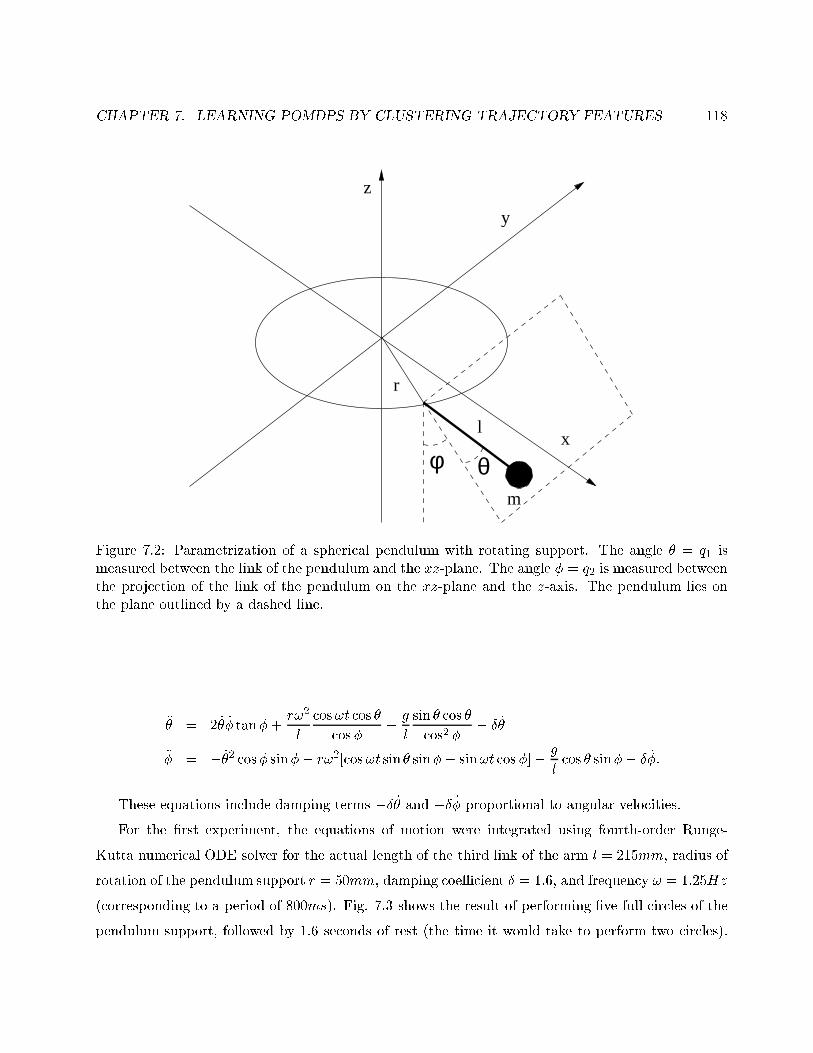
CHAPTER 7. LEARNING POMDPS BY CLUSTERING TRAJECTORY FEATURES 118
x
y
z
r
l
m
θφ
Figure 7.2: Parametrization of a spherical pendulum with rotating support. The angle � = q1 ismeasured between the link of the pendulum and the xz-plane. The angle � = q2 is measured betweenthe projection of the link of the pendulum on the xz-plane and the z-axis. The pendulum lies onthe plane outlined by a dashed line.
�� = 2 _� _� tan�+r!2
l
cos!t cos �
cos��g
l
sin � cos �
cos2 �� Æ _�
�� = � _�2 cos� sin�� r!2[cos!t sin � sin�� sin!t cos�]�g
lcos � sin�� Æ _�:
These equations include damping terms �Æ _� and �Æ _� proportional to angular velocities.
For the �rst experiment, the equations of motion were integrated using fourth-order Runge-
Kutta numerical ODE solver for the actual length of the third link of the arm l = 215mm, radius of
rotation of the pendulum support r = 50mm, damping coeÆcient Æ = 1:6, and frequency ! = 1:25Hz
(corresponding to a period of 800ms). Fig. 7.3 shows the result of performing �ve full circles of the
pendulum support, followed by 1:6 seconds of rest (the time it would take to perform two circles).
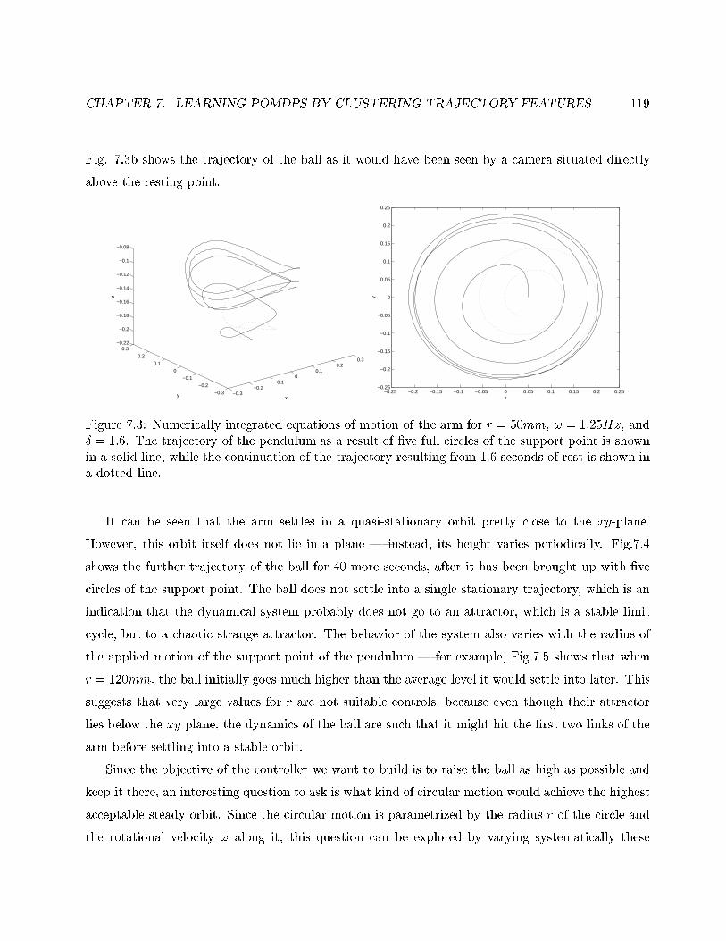
CHAPTER 7. LEARNING POMDPS BY CLUSTERING TRAJECTORY FEATURES 119
Fig. 7.3b shows the trajectory of the ball as it would have been seen by a camera situated directly
above the resting point.
−0.3−0.2
−0.10
0.10.2
0.3
−0.3
−0.2
−0.1
0
0.1
0.2
0.3−0.22
−0.2
−0.18
−0.16
−0.14
−0.12
−0.1
−0.08
xy
z
−0.25 −0.2 −0.15 −0.1 −0.05 0 0.05 0.1 0.15 0.2 0.25−0.25
−0.2
−0.15
−0.1
−0.05
0
0.05
0.1
0.15
0.2
0.25
x
y
Figure 7.3: Numerically integrated equations of motion of the arm for r = 50mm, ! = 1:25Hz, andÆ = 1:6. The trajectory of the pendulum as a result of �ve full circles of the support point is shownin a solid line, while the continuation of the trajectory resulting from 1:6 seconds of rest is shown ina dotted line.
It can be seen that the arm settles in a quasi-stationary orbit pretty close to the xy-plane.
However, this orbit itself does not lie in a plane | instead, its height varies periodically. Fig.7.4
shows the further trajectory of the ball for 40 more seconds, after it has been brought up with �ve
circles of the support point. The ball does not settle into a single stationary trajectory, which is an
indication that the dynamical system probably does not go to an attractor, which is a stable limit
cycle, but to a chaotic strange attractor. The behavior of the system also varies with the radius of
the applied motion of the support point of the pendulum | for example, Fig.7.5 shows that when
r = 120mm, the ball initially goes much higher than the average level it would settle into later. This
suggests that very large values for r are not suitable controls, because even though their attractor
lies below the xy plane, the dynamics of the ball are such that it might hit the �rst two links of the
arm before settling into a stable orbit.
Since the objective of the controller we want to build is to raise the ball as high as possible and
keep it there, an interesting question to ask is what kind of circular motion would achieve the highest
acceptable steady orbit. Since the circular motion is parametrized by the radius r of the circle and
the rotational velocity ! along it, this question can be explored by varying systematically these
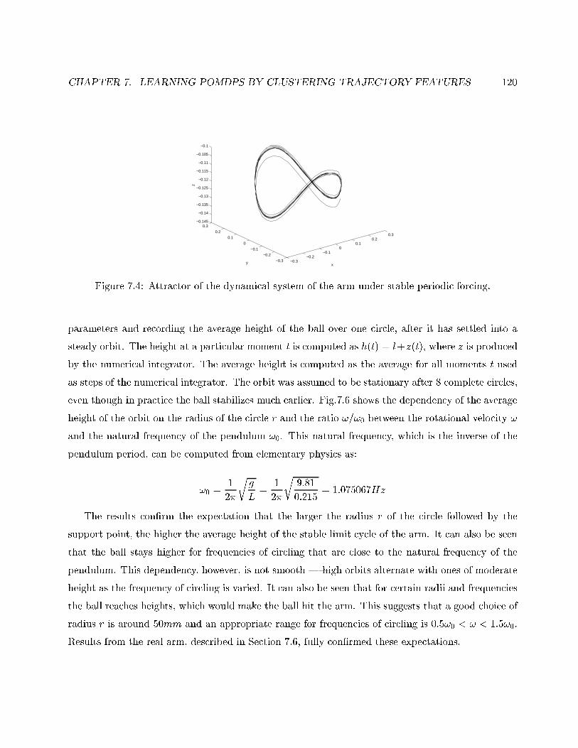
CHAPTER 7. LEARNING POMDPS BY CLUSTERING TRAJECTORY FEATURES 120
−0.3−0.2
−0.10
0.10.2
0.3
−0.3
−0.2
−0.1
0
0.1
0.2
0.3−0.145
−0.14
−0.135
−0.13
−0.125
−0.12
−0.115
−0.11
−0.105
−0.1
xy
z
Figure 7.4: Attractor of the dynamical system of the arm under stable periodic forcing.
parameters and recording the average height of the ball over one circle, after it has settled into a
steady orbit. The height at a particular moment t is computed as h(t) = l+z(t), where z is produced
by the numerical integrator. The average height is computed as the average for all moments t used
as steps of the numerical integrator. The orbit was assumed to be stationary after 8 complete circles,
even though in practice the ball stabilizes much earlier. Fig.7.6 shows the dependency of the average
height of the orbit on the radius of the circle r and the ratio !=!0 between the rotational velocity !
and the natural frequency of the pendulum !0. This natural frequency, which is the inverse of the
pendulum period, can be computed from elementary physics as:
!0 =1
2�
rg
L=
1
2�
r9:81
0:215= 1:075067Hz
The results con�rm the expectation that the larger the radius r of the circle followed by the
support point, the higher the average height of the stable limit cycle of the arm. It can also be seen
that the ball stays higher for frequencies of circling that are close to the natural frequency of the
pendulum. This dependency, however, is not smooth | high orbits alternate with ones of moderate
height as the frequency of circling is varied. It can also be seen that for certain radii and frequencies
the ball reaches heights, which would make the ball hit the arm. This suggests that a good choice of
radius r is around 50mm and an appropriate range for frequencies of circling is 0:5!0 < ! < 1:5!0.
Results from the real arm, described in Section 7.6, fully con�rmed these expectations.
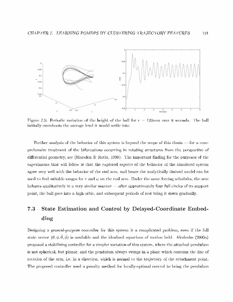
CHAPTER 7. LEARNING POMDPS BY CLUSTERING TRAJECTORY FEATURES 121
−0.5
0
0.5
−0.5
0
0.5−0.25
−0.2
−0.15
−0.1
−0.05
0
xy
z
0 1 2 3 4 5 6 7 8−0.25
−0.2
−0.15
−0.1
−0.05
0
time [sec]
z [m
]Figure 7.5: Periodic variation of the height of the ball for r = 120mm over 8 seconds. The ballinitially overshoots the average level it would settle into.
Further analysis of the behavior of this system is beyond the scope of this thesis | for a com-
prehensive treatment of the bifurcations occurring in rotating structures from the perspective of
di�erential geometry, see (Marsden & Ratiu, 1998). The important �nding for the purposes of the
experiments that will follow is that the explored aspects of the behavior of the simulated system
agree very well with the behavior of the real arm, and hence the analytically derived model can be
used to �nd suitable ranges for r and ! on the real arm. Under the same forcing schedules, the arm
behaves qualitatively in a very similar manner | after approximately four full circles of its support
point, the ball goes into a high orbit, and subsequent periods of rest bring it down gradually.
7.3 State Estimation and Control by Delayed-Coordinate Embed-
ding
Designing a general-purpose controller for this system is a complicated problem, even if the full
state vector (�; �; _�; _�) is available and the idealized equations of motion held. Akulenko (2000a)
proposed a stabilizing controller for a simpler variation of this system, where the attached pendulum
is not spherical, but planar, and the pendulum always swings in a plane which contains the line of
rotation of the arm, i.e, in a direction, which is normal to the trajectory of the attachment point.
The proposed controller used a penalty method for locally-optimal control to bring the pendulum
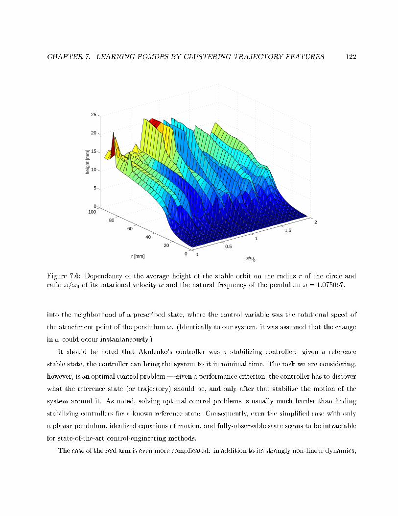
CHAPTER 7. LEARNING POMDPS BY CLUSTERING TRAJECTORY FEATURES 122
0
0.5
1
1.5
2
0
20
40
60
80
1000
5
10
15
20
25
ω/ω0
r [mm]
heig
ht [m
m]
Figure 7.6: Dependency of the average height of the stable orbit on the radius r of the circle andratio !=!0 of its rotational velocity ! and the natural frequency of the pendulum ! = 1:075067.
into the neighborhood of a prescribed state, where the control variable was the rotational speed of
the attachment point of the pendulum !. (Identically to our system, it was assumed that the change
in ! could occur instantaneously.)
It should be noted that Akulenko's controller was a stabilizing controller: given a reference
stable state, the controller can bring the system to it in minimal time. The task we are considering,
however, is an optimal control problem| given a performance criterion, the controller has to discover
what the reference state (or trajectory) should be, and only after that stabilize the motion of the
system around it. As noted, solving optimal control problems is usually much harder than �nding
stabilizing controllers for a known reference state. Consequently, even the simpli�ed case with only
a planar pendulum, idealized equations of motion, and fully-observable state seems to be intractable
for state-of-the-art control-engineering methods.
The case of the real arm is even more complicated: in addition to its strongly non-linear dynamics,
CHAPTER 7. LEARNING POMDPS BY CLUSTERING TRAJECTORY FEATURES 123
the links are not completely rigid, and the signi�cant mass of the ball in comparison with the
servo torques interacts with the links in ways, which are hard to capture in a dynamical model.
Furthermore, although the kinematics of the arm are known, the camera is not calibrated and the
actual state of the system cannot be inferred; such a model is not even possible, because estimating
the state of a ball ying in three-dimensional space from a single camera image is an ill-posed
problem. Even if estimating the position was possible, the frame rate is too low to estimate the
translational and rotational velocities of the ball by frame di�erencing. Finally, there are occasional
delays in control periods, which, although small and infrequent, can have signi�cant impact on
the ight of the ball. All of these factors make the state of the system only partially observable,
which, combined with its strong nonlinearity, makes the application of traditional control algorithms
virtually impossible.
However, in spite of the seemingly insurmountable complexity of this problem from a control-
engineering standpoint, it is clear that the qualitative behavior of the system is actually quite simple:
periodic motion of the support adds energy to the ball and as a result it goes up; when the support
point does not move, the ball continues circling on its momentum, dropping down under the in uence
of gravity and air friction. Such a behavior is quite similar to Watt's centrifugal governor, whose
height is regulated by its angular velocity of rotation. The analysis of the system in simulation in
the previous section indicated that a circular motion of the attachment point of the third link with a
suitable frequency ! and radius r can bring the ball into a steady orbit as high as physically possible,
without exceeding the height of the plane where the arm moves, and if the arm stops, the ball goes
down while still circling steadily. The previous section also identi�ed the neighborhood in which
suitable parameters ! and r can be found.
This suggests that a policy which would achieve high performance, while being energy eÆcient
at the same time, could consist of alternating circles of appropriate amplitude and frequency with
periods of rest, when the ball continues circling on momentum while still preserving most of its height.
The problem then becomes how to switch between a powerful, but expensive control a, which almost
always succeeds in bringing the ball to a high orbit and keeping it there, and a weak control b, which
is inexpensive, but still retains good performance if the ball already has some momentum. This is
a closed-loop control problem, because the application of the weak control b a�ects the behavior of
the ball very di�erently at di�erent heights, and a controller has to consider the state of the ball
when deciding whether to apply controls a or b. In particular, control b certainly results in zero
CHAPTER 7. LEARNING POMDPS BY CLUSTERING TRAJECTORY FEATURES 124
performance when the ball is at rest, and is only useful when the ball already has some momentum.
Furthermore, experiments with the real arm showed that if the ball is dropped too low, subsequent
application of the powerful control a often fails to raise the height of the ball and might result in
chaotic behavior.
This is also a sequential decision problem, because it usually takes at least 4 circles to raise the
ball to a steady orbit, and similarly, it takes more than 5 periods of inaction to drop the ball close
to its resting state. Decisions about which action to apply must take into consideration the future
evolution of the state of the system, which can only be done by an optimal sequential controller.
In general, the task of the controller is to bring the ball up initially by applying a several times,
and once it is high enough, use the momentum of the ball to conserve energy by applying action b.
However, as soon as the ball drops down to a level, which is likely to result in chaotic behavior, the
controller should bring it back up by applying action a. As noted, designing such a controller by
means of general control-engineering methodology is very hard or impossible.
The alternative approach pursued in this thesis is to collect an execution trace by following a
suitable exploration policy, learn a probabilistic model of the dynamics of the system so as to model
the execution trace well, and use this model for planning and optimal control. The mobile robot
navigation task discussed in the previous two chapters employed learning algorithms that learned a
true POMDP model with hidden variables. The characteristics of the task considered in this chapter,
however, allow for a di�erent method of building probabilistic models. This method learns a fully-
observable MDP (FOMDP) model of a partially-observable MDP. How and why this is possible is
discussed below.
While localization on mobile robots requires arbitrarily long sequences of past percepts to be
considered by both learning and reasoning algorithms, the dynamics of the ball control task permit
only �nite sequences to be considered when building the model. The reason for this is the low
dimensionality of the system constrained by the actions described above | as discussed, its e�ective
con�guration space is two dimensional (described by the vector (�, �)), and hence its state space is
four dimensional (described by the vector (�, �, _�, _�)).
The much celebrated theorem of Takens (1980; 1985) states that if the dimension of a dynamical
system is d, an embedding space of no more than 2d + 1 delayed outputs of the system contains a
manifold that can be put into one-to-one correspondence (di�eomorphism) with the attractor of the
dynamical system, and this correspondence is smooth if the state transition function of the system
CHAPTER 7. LEARNING POMDPS BY CLUSTERING TRAJECTORY FEATURES 125
is itself smooth. Assuming that the observation function of the system is smooth too, a consequence
of this theorem is that the mapping from a window of 2d + 1 delayed outputs of the system to
the next output is a di�eomorphism too. Sauer et al. (1991) further developed the proof and
employed it very successfully for time series prediction by using a locally-linear regression to learn
the di�eomorphic mapping (Sauer, 1993). This theorem is also the theoretical foundation behind
the use of time-delayed neural networks.
The theorem is also compatible with our approach to state identi�cation and learning. Consider
two consecutive windows (intervals) of size 2d+1 percepts ordered in time, where action a1 2 fa; bg
is performed during the �rst window, and action a2 2 fa; bg is performed during the second window.
Applying the theorem to the percepts in the �rst window, it follows that there exists a di�eomorphism
between the percepts in that window (the inputs) and the �rst percept in the second window (the
output). Now shift the input window one time step forward in time, and apply the theorem to
the new window, which now consists of 2d percepts from the �rst interval and the �rst percept
from the second interval. Using the property that the composition of two smooth functions is a
smooth function, it follows that there is a di�eomorphism between the new window and the second
percept in the second interval. Reasoning analogously, it can be concluded that a (vector-valued)
di�eomorphism exists between the �rst and second interval windows.
The net result of this reasoning is that the unknown system, which has d-dimensional hidden
state space and any number of observation variables, can be replaced by another system with fully-
observable 2d+1-dimensional state space and identical behavior. The state of the newly constructed
system consists of ordered windows of length 2d + 1 of past observations. This result is guaranteed
even when there is only a single observation variable to use in the delayed-coordinate embedding. It
has been reported, though, that in practice having more than one observation variable can help the
reconstruction of the system a lot when the training data are noisy, and possibly allow embedding
spaces of dimension less than 2d+ 1 to be used (Honkela, 2001).
The delayed-coordinate embedding approach is pervasive in the area of system identi�cation,
where it forms the basis of subspace identi�cation methods for linear systems such as CVA (Larimore,
1990) and N4SID (Overschee & Moor, 1994), which de�ne the state of the art in that area. These
algorithms also use the fact that compositions of linear functions can be factored in a canonical way
by means of Singular Value Decomposition to recover separate transition and observation functions.
For arbitrary nonlinear systems, however, such a factorization is not possible. Also, as noted in
CHAPTER 7. LEARNING POMDPS BY CLUSTERING TRAJECTORY FEATURES 126
Chapter 2, even if it was possible to recover a full nonlinear state-space model in the form of a set
of ODEs, there are no general methods for solving the resulting Hamilton-Jacobi-Bellman equations
of optimal control, and only progress on solving relatively simple systems has been made (Munos &
Moore, 1998). Even the analytically derived equations of motion of the spherical pendulum are well
beyond the capabilities of currently available methods, left alone a model learned from observation
data.
If we use delayed-coordinate embedding, however, we turn the system into fully observable, even
though with unknown system dynamics. Solving sequential decision problems for such systems is
the domain of reinforcement learning in continuous state spaces. A solution that is very similar to
the state merging approach we are pursuing has been proposed by Mahadevan and Connell (1992).
They solved a hard reinforcement learning problem in 144-dimensional fully observable state space,
where local occupancy grids around a mobile robot served as state. The key to dealing with high-
dimensional continuous state spaces in their solution was to merge sample states into clusters, which
is very similar to the state-aggregation approach explored in the previous two chapters. This is the
approach we use for the ying ball problem as well.
7.4 Learning a FOMDP Model by Delayed-Coordinate Embedding
We ground a small set of discrete states into feature space by means of clustering features of the
starting states in the execution trace, and subsequently estimate the transition probabilities between
clusters under all actions. The rationale behind this approach is that a clustering algorithm naturally
produces clusters of states aggregated in regions with high occupancy, which results in approximately
even distribution among clusters of the samples, from which transition matrices are estimated, and
thus in higher precision of the estimates. On the contrary, a uniform discretization of feature space,
which is not driven by the actual experienced trajectories, is likely to result in imprecise frequency
counts and thus in high variance of the estimates. Furthermore, uniform discretization of a high-
dimensional space derived by means of delayed-coordinate embedding would result in a combinatorial
explosion and the well known curse of dimensionality.
Currently, the algorithm uses a �xed predetermined number Ns of clusters. This number depends
on the number N of sampled transitions in the execution trace { if we assume a relatively even
distribution of starting states among clusters, then an average of N=Ns states are likely to appear to
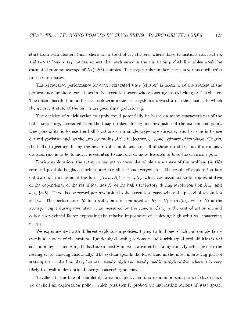
CHAPTER 7. LEARNING POMDPS BY CLUSTERING TRAJECTORY FEATURES 127
start from each cluster. Since there are a total of Ns clusters, where these transitions can lead to,
and two actions to try, we can expect that each entry in the transition probability tables would be
estimated from an average of N=(2N2s ) samples. The larger this number, the less variance will exist
in these estimates.
The aggregated performance for each aggregated state (cluster) is taken to be the average of the
performance for those transitions in the execution trace, whose starting states belong to this cluster.
The initial distribution in this case is deterministic { the system always starts in the cluster, to which
the quiescent state of the ball is assigned during clustering.
The decision of which action to apply could potentially be based on many characteristics of the
ball's trajectory, measured from the images taken during one revolution of the attachment point.
One possibility is to use the ball locations on a single trajectory directly; another one is to use
derived statistics such as the average radius of the trajectory, or some estimate of its phase. Clearly,
the ball's trajectory during the next revolution depends on all of these variables, but if a compact
decision rule is to be found, it is essential to �nd one or more features to base the decision upon.
During exploration, the system attempts to cover the whole state space of the problem (in this
case, all possible heights of orbit), and try all actions everywhere. The result of exploration is a
database of transitions of the form (Xi; ai; Ri), i = 1; No, which are assumed to be representative
of the dependency of the set of features Xi of the ball's trajectory during revolution i on Xi�1 and
ai 2 fa; bg. There is one record per revolution in the execution trace, where the period of revolution
is 1=!. The performance Ri for revolution i is computed as Ri = �Hi � �C(ai), where �Hi is the
average height during revolution i, as measured by the camera, C(ai) is the cost of action ai, and
� is a user-de�ned factor expressing the relative importance of achieving high orbit vs. conserving
energy.
We experimented with di�erent exploration policies, trying to �nd one which can sample fairly
evenly all modes of the system. Randomly choosing actions a and b with equal probabilities is not
such a policy | under it, the ball stays mostly in two states: either in high steady orbit, or near the
resting state, moving chaotically. The system spends the least time in the most interesting part of
state space | the boundary between steady high and steady medium-high orbits, where it is very
likely to dwell under optimal energy-conserving policies.
To alleviate this bias of completely random exploration towards unimportant parts of state space,
we devised an exploration policy, which persistently probed the interesting regions of state space.
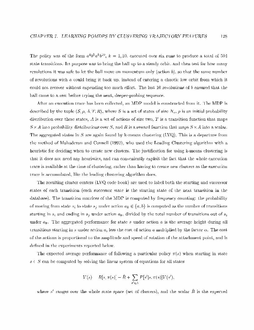
CHAPTER 7. LEARNING POMDPS BY CLUSTERING TRAJECTORY FEATURES 128
The policy was of the form a4bkakb10, k = 1; 10, executed over six runs to produce a total of 504
state transitions. Its purpose was to bring the ball up to a steady orbit, and then test for how many
revolutions it was safe to let the ball move on momentum only (action b), so that the same number
of revolutions with a could bring it back up, instead of entering a chaotic low orbit from which it
could not recover without expending too much e�ort. The last 10 revolutions of b ensured that the
ball came to a rest before trying the next, deeper-probing sequence.
After an execution trace has been collected, an MDP model is constructed from it. The MDP is
described by the tuple (S; �;A; T;R), where S is a set of states of size Ns, � is an initial probability
distribution over these states, A is a set of actions of size two, T is a transition function that maps
S�A into probability distributions over S, and R is a reward function that maps S�A into a scalar.
The aggregated states in S are again found by k-means clustering (LVQ). This is a departure from
the method of Mahadevan and Connell (1992), who used the Leading Clustering algorithm with a
heuristic for deciding when to create new clusters. The justi�cation for using k-means clustering is
that it does not need any heuristics, and can conveniently exploit the fact that the whole execution
trace is available at the time of clustering, rather than having to create new clusters as the execution
trace is accumulated, like the leading clustering algorithm does.
The resulting cluster centers (LVQ code book) are used to label both the starting and successor
states of each transition (each successor state is the starting state of the next transition in the
database). The transition matrices of the MDP is computed by frequency counting: the probability
of moving from state si to state sj under action ak 2 fa; bg is computed as the number of transitions
starting in si and ending in sj under action ak, divided by the total number of transitions out of si
under ak. The aggregated performance for state s under action a is the average height during all
transitions starting in s under action a, less the cost of action a multiplied by the factor �. The cost
of the actions is proportional to the amplitude and speed of rotation of the attachment point, and is
de�ned in the experiments reported below.
The expected average performance of following a particular policy �(s) when starting in state
s 2 S can be computed by solving the linear system of equations for all states
V (s) = R[s; �(s)]� R+Xs02S
P [s0js; �(s)]V (s0);
where s0 ranges over the whole state space (set of clusters), and the scalar R is the expected
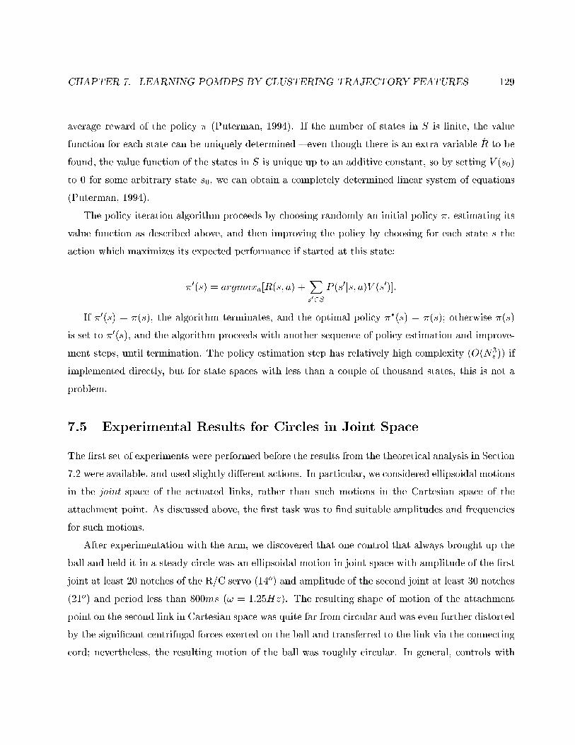
CHAPTER 7. LEARNING POMDPS BY CLUSTERING TRAJECTORY FEATURES 129
average reward of the policy � (Puterman, 1994). If the number of states in S is �nite, the value
function for each state can be uniquely determined { even though there is an extra variable R to be
found, the value function of the states in S is unique up to an additive constant, so by setting V (s0)
to 0 for some arbitrary state s0, we can obtain a completely determined linear system of equations
(Puterman, 1994).
The policy iteration algorithm proceeds by choosing randomly an initial policy �, estimating its
value function as described above, and then improving the policy by choosing for each state s the
action which maximizes its expected performance if started at this state:
�0(s) = argmaxa[R(s; a) +Xs02S
P (s0js; a)V (s0)]:
If �0(s) = �(s), the algorithm terminates, and the optimal policy ��(s) = �(s); otherwise �(s)
is set to �0(s), and the algorithm proceeds with another sequence of policy estimation and improve-
ment steps, until termination. The policy estimation step has relatively high complexity (O(N3s )) if
implemented directly, but for state spaces with less than a couple of thousand states, this is not a
problem.
7.5 Experimental Results for Circles in Joint Space
The �rst set of experiments were performed before the results from the theoretical analysis in Section
7.2 were available, and used slightly di�erent actions. In particular, we considered ellipsoidal motions
in the joint space of the actuated links, rather than such motions in the Cartesian space of the
attachment point. As discussed above, the �rst task was to �nd suitable amplitudes and frequencies
for such motions.
After experimentation with the arm, we discovered that one control that always brought up the
ball and held it in a steady circle was an ellipsoidal motion in joint space with amplitude of the �rst
joint at least 20 notches of the R/C servo (14o) and amplitude of the second joint at least 30 notches
(21o) and period less than 800ms (! = 1:25Hz). The resulting shape of motion of the attachment
point on the second link in Cartesian space was quite far from circular and was even further distorted
by the signi�cant centrifugal forces exerted on the ball and transferred to the link via the connecting
cord; nevertheless, the resulting motion of the ball was roughly circular. In general, controls with
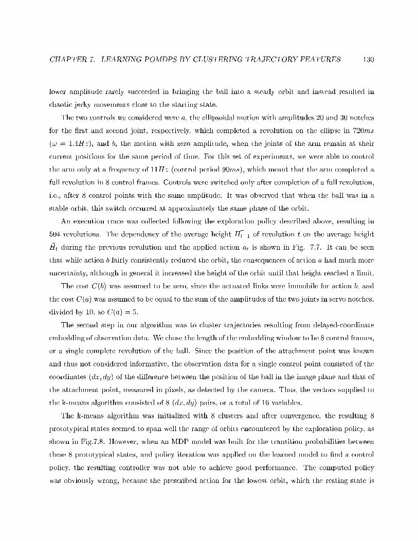
CHAPTER 7. LEARNING POMDPS BY CLUSTERING TRAJECTORY FEATURES 130
lower amplitude rarely succeeded in bringing the ball into a steady orbit and instead resulted in
chaotic jerky movements close to the starting state.
The two controls we considered were a, the ellipsoidal motion with amplitudes 20 and 30 notches
for the �rst and second joint, respectively, which completed a revolution on the ellipse in 720ms
(! = 1:4Hz), and b, the motion with zero amplitude, when the joints of the arm remain at their
current positions for the same period of time. For this set of experiments, we were able to control
the arm only at a frequency of 11Hz (control period 90ms), which meant that the arm completed a
full revolution in 8 control frames. Controls were switched only after completion of a full revolution,
i.e., after 8 control points with the same amplitude. It was observed that when the ball was in a
stable orbit, this switch occurred at approximately the same phase of the orbit.
An execution trace was collected following the exploration policy described above, resulting in
504 revolutions. The dependency of the average height �Ht+1 of revolution t on the average height
�Ht during the previous revolution and the applied action at is shown in Fig. 7.7. It can be seen
that while action b fairly consistently reduced the orbit, the consequences of action a had much more
uncertainty, although in general it increased the height of the orbit until that height reached a limit.
The cost C(b) was assumed to be zero, since the actuated links were immobile for action b, and
the cost C(a) was assumed to be equal to the sum of the amplitudes of the two joints in servo notches,
divided by 10, so C(a) = 5.
The second step in our algorithm was to cluster trajectories resulting from delayed-coordinate
embedding of observation data. We chose the length of the embedding window to be 8 control frames,
or a single complete revolution of the ball. Since the position of the attachment point was known
and thus not considered informative, the observation data for a single control point consisted of the
coordinates (dx; dy) of the di�erence between the position of the ball in the image plane and that of
the attachment point, measured in pixels, as detected by the camera. Thus, the vectors supplied to
the k-means algorithm consisted of 8 (dx; dy) pairs, or a total of 16 variables.
The k-means algorithm was initialized with 8 clusters and after convergence, the resulting 8
prototypical states seemed to span well the range of orbits encountered by the exploration policy, as
shown in Fig.7.8. However, when an MDP model was built for the transition probabilities between
these 8 prototypical states, and policy iteration was applied on the learned model to �nd a control
policy, the resulting controller was not able to achieve good performance. The computed policy
was obviously wrong, because the prescribed action for the lowest orbit, which the resting state is
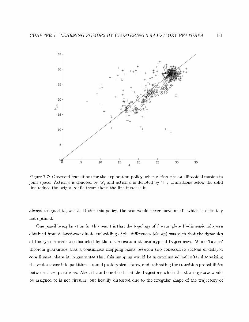
CHAPTER 7. LEARNING POMDPS BY CLUSTERING TRAJECTORY FEATURES 131
0 5 10 15 20 25 30 350
5
10
15
20
25
30
35
Hi
Hi+
1
Figure 7.7: Observed transitions for the exploration policy, when action a is an ellipsoidal motion injoint space. Action b is denoted by 'o', and action a is denoted by '+'. Transitions below the solidline reduce the height, while those above the line increase it.
always assigned to, was b. Under this policy, the arm would never move at all, which is de�nitely
not optimal.
One possible explanation for this result is that the topology of the complete 16-dimensional space
obtained from delayed-coordinate embedding of the di�erences (dx; dy) was such that the dynamics
of the system were too distorted by the discretization at prototypical trajectories. While Takens'
theorem guarantees that a continuous mapping exists between two consecutive vectors of delayed
coordinates, there is no guarantee that this mapping would be approximated well after discretizing
the vector space into partitions around prototypical states, and estimating the transition probabilities
between these partitions. Also, it can be noticed that the trajectory which the starting state would
be assigned to is not circular, but heavily distorted due to the irregular shape of the trajectory of
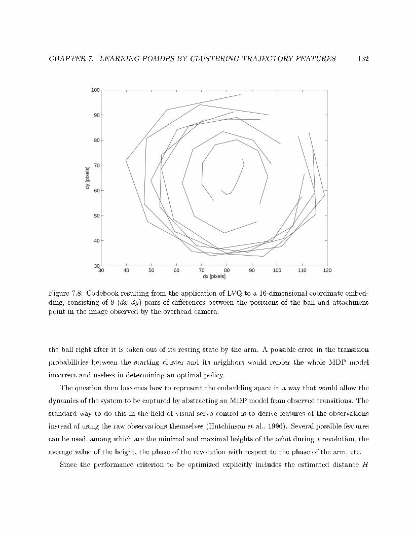
CHAPTER 7. LEARNING POMDPS BY CLUSTERING TRAJECTORY FEATURES 132
30 40 50 60 70 80 90 100 110 12030
40
50
60
70
80
90
100
dx [pixels]
dy [p
ixel
s]
Figure 7.8: Codebook resulting from the application of LVQ to a 16-dimensional coordinate embed-ding, consisting of 8 (dx; dy) pairs of di�erences between the positions of the ball and attachmentpoint in the image observed by the overhead camera.
the ball right after it is taken out of its resting state by the arm. A possible error in the transition
probabilities between the starting cluster and its neighbors would render the whole MDP model
incorrect and useless in determining an optimal policy.
The question then becomes how to represent the embedding space in a way that would allow the
dynamics of the system to be captured by abstracting an MDP model from observed transitions. The
standard way to do this in the �eld of visual servo control is to derive features of the observations
instead of using the raw observations themselves (Hutchinson et al., 1996). Several possible features
can be used, among which are the minimal and maximal heights of the orbit during a revolution, the
average value of the height, the phase of the revolution with respect to the phase of the arm, etc.
Since the performance criterion to be optimized explicitly includes the estimated distance H
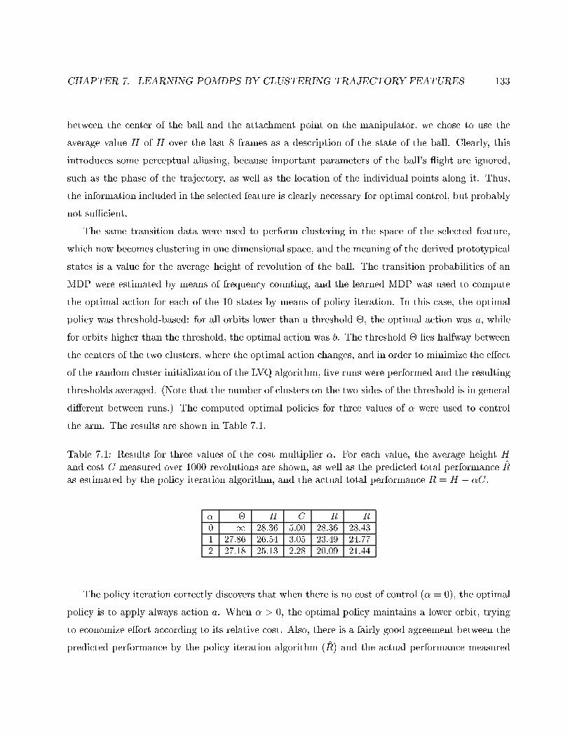
CHAPTER 7. LEARNING POMDPS BY CLUSTERING TRAJECTORY FEATURES 133
between the center of the ball and the attachment point on the manipulator, we chose to use the
average value �H of H over the last 8 frames as a description of the state of the ball. Clearly, this
introduces some perceptual aliasing, because important parameters of the ball's ight are ignored,
such as the phase of the trajectory, as well as the location of the individual points along it. Thus,
the information included in the selected feature is clearly necessary for optimal control, but probably
not suÆcient.
The same transition data were used to perform clustering in the space of the selected feature,
which now becomes clustering in one dimensional space, and the meaning of the derived prototypical
states is a value for the average height of revolution of the ball. The transition probabilities of an
MDP were estimated by means of frequency counting, and the learned MDP was used to compute
the optimal action for each of the 10 states by means of policy iteration. In this case, the optimal
policy was threshold-based: for all orbits lower than a threshold �, the optimal action was a, while
for orbits higher than the threshold, the optimal action was b. The threshold � lies halfway between
the centers of the two clusters, where the optimal action changes, and in order to minimize the e�ect
of the random cluster initialization of the LVQ algorithm, �ve runs were performed and the resulting
thresholds averaged. (Note that the number of clusters on the two sides of the threshold is in general
di�erent between runs.) The computed optimal policies for three values of � were used to control
the arm. The results are shown in Table 7.1.
Table 7.1: Results for three values of the cost multiplier �. For each value, the average height �Hand cost �C measured over 1000 revolutions are shown, as well as the predicted total performance Ras estimated by the policy iteration algorithm, and the actual total performance �R = �H � � �C.
� � �H �C �R R
0 1 28:36 5:00 28:36 28:43
1 27:86 26:54 3:05 23:49 24:77
2 27:18 25:13 2:28 20:09 21:44
The policy iteration correctly discovers that when there is no cost of control (� = 0), the optimal
policy is to apply always action a. When � > 0, the optimal policy maintains a lower orbit, trying
to economize e�ort according to its relative cost. Also, there is a fairly good agreement between the
predicted performance by the policy iteration algorithm (R) and the actual performance measured
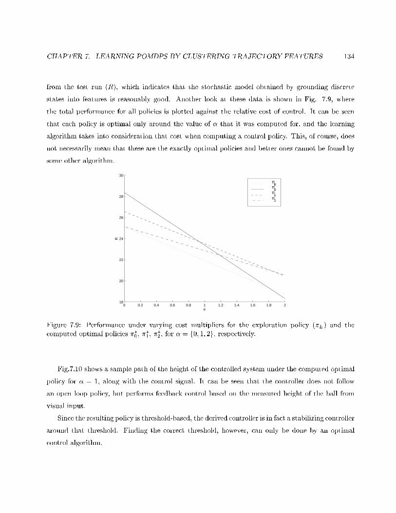
CHAPTER 7. LEARNING POMDPS BY CLUSTERING TRAJECTORY FEATURES 134
from the test run ( �R), which indicates that the stochastic model obtained by grounding discrete
states into features is reasonably good. Another look at these data is shown in Fig. 7.9, where
the total performance for all policies is plotted against the relative cost of control. It can be seen
that each policy is optimal only around the value of � that it was computed for, and the learning
algorithm takes into consideration that cost when computing a control policy. This, of course, does
not necessarily mean that these are the exactly optimal policies and better ones cannot be found by
some other algorithm.
0 0.2 0.4 0.6 0.8 1 1.2 1.4 1.6 1.8 218
20
22
24
26
28
30
α
R
πE
π*0
π*1
π*2
Figure 7.9: Performance under varying cost multipliers for the exploration policy (�E) and thecomputed optimal policies ��0, �
�1, �
�2, for � = f0; 1; 2g, respectively.
Fig.7.10 shows a sample path of the height of the controlled system under the computed optimal
policy for � = 1, along with the control signal. It can be seen that the controller does not follow
an open loop policy, but performs feedback control based on the measured height of the ball from
visual input.
Since the resulting policy is threshold-based, the derived controller is in fact a stabilizing controller
around that threshold. Finding the correct threshold, however, can only be done by an optimal
control algorithm.
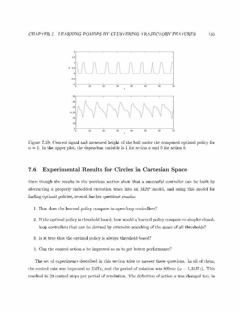
CHAPTER 7. LEARNING POMDPS BY CLUSTERING TRAJECTORY FEATURES 135
0 10 20 30 40 50 60 70−1
−0.5
0
0.5
1
1.5
2
t
a
0 10 20 30 40 50 60 705
10
15
20
25
30
35
t
H
Figure 7.10: Control signal and measured height of the ball under the computed optimal policy for� = 1. In the upper plot, the dependent variable is 1 for action a and 0 for action b.
7.6 Experimental Results for Circles in Cartesian Space
Even though the results in the previous section show that a successful controller can be built by
abstracting a properly embedded execution trace into an MDP model, and using this model for
�nding optimal policies, several further questions remain:
1. How does the learned policy compare to open-loop controllers?
2. If the optimal policy is threshold based, how would a learned policy compare to simpler closed-
loop controllers that can be derived by extensive searching of the space of all thresholds?
3. Is it true that the optimal policy is always threshold-based?
4. Can the control action a be improved so as to get better performance?
The set of experiments described in this section tries to answer these questions. In all of them,
the control rate was improved to 25Hz, and the period of rotation was 800ms (! = 1:25Hz). This
resulted in 20 control steps per period of revolution. The de�nition of action a was changed too, in
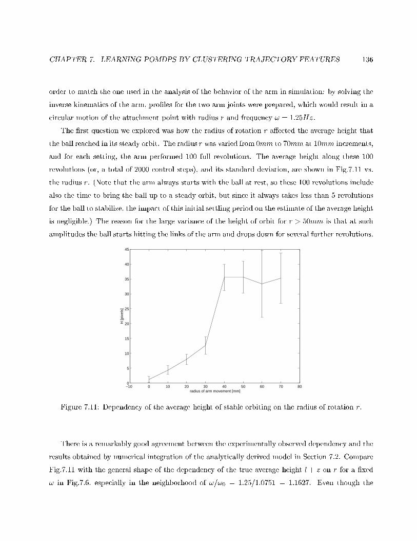
CHAPTER 7. LEARNING POMDPS BY CLUSTERING TRAJECTORY FEATURES 136
order to match the one used in the analysis of the behavior of the arm in simulation: by solving the
inverse kinematics of the arm, pro�les for the two arm joints were prepared, which would result in a
circular motion of the attachment point with radius r and frequency ! = 1:25Hz.
The �rst question we explored was how the radius of rotation r a�ected the average height that
the ball reached in its steady orbit. The radius r was varied from 0mm to 70mm at 10mm increments,
and for each setting, the arm performed 100 full revolutions. The average height along these 100
revolutions (or, a total of 2000 control steps), and its standard deviation, are shown in Fig.7.11 vs.
the radius r. (Note that the arm always starts with the ball at rest, so these 100 revolutions include
also the time to bring the ball up to a steady orbit, but since it always takes less than 5 revolutions
for the ball to stabilize, the impact of this initial settling period on the estimate of the average height
is negligible.) The reason for the large variance of the height of orbit for r > 50mm is that at such
amplitudes the ball starts hitting the links of the arm and drops down for several further revolutions.
−10 0 10 20 30 40 50 60 70 800
5
10
15
20
25
30
35
40
45
radius of arm movement [mm]
H [p
ixel
s]
Figure 7.11: Dependency of the average height of stable orbiting on the radius of rotation r.
There is a remarkably good agreement between the experimentally observed dependency and the
results obtained by numerical integration of the analytically derived model in Section 7.2. Compare
Fig.7.11 with the general shape of the dependency of the true average height l + z on r for a �xed
! in Fig.7.6, especially in the neighborhood of !=!0 = 1:25=1:0751 = 1:1627. Even though the
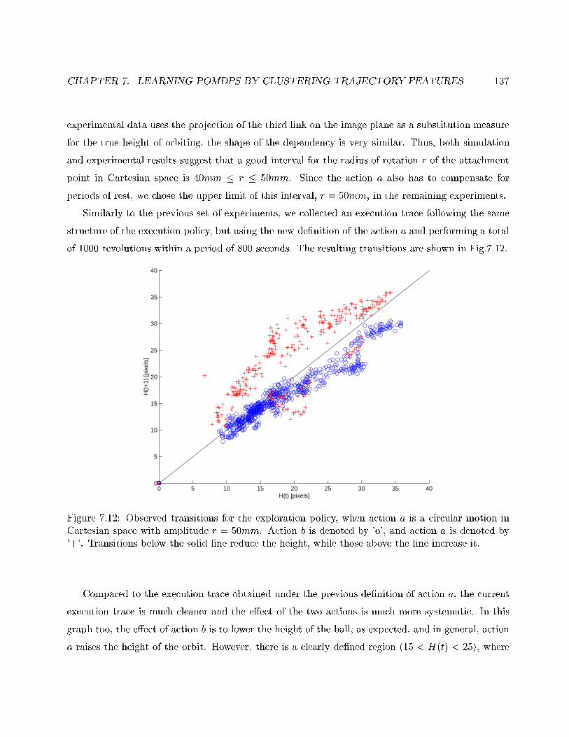
CHAPTER 7. LEARNING POMDPS BY CLUSTERING TRAJECTORY FEATURES 137
experimental data uses the projection of the third link on the image plane as a substitution measure
for the true height of orbiting, the shape of the dependency is very similar. Thus, both simulation
and experimental results suggest that a good interval for the radius of rotation r of the attachment
point in Cartesian space is 40mm � r � 50mm. Since the action a also has to compensate for
periods of rest, we chose the upper limit of this interval, r = 50mm, in the remaining experiments.
Similarly to the previous set of experiments, we collected an execution trace following the same
structure of the execution policy, but using the new de�nition of the action a and performing a total
of 1000 revolutions within a period of 800 seconds. The resulting transitions are shown in Fig.7.12.
0 5 10 15 20 25 30 35 400
5
10
15
20
25
30
35
40
H(t) [pixels]
H(t
+1)
[pix
els]
Figure 7.12: Observed transitions for the exploration policy, when action a is a circular motion inCartesian space with amplitude r = 50mm. Action b is denoted by 'o', and action a is denoted by'+'. Transitions below the solid line reduce the height, while those above the line increase it.
Compared to the execution trace obtained under the previous de�nition of action a, the current
execution trace is much cleaner and the e�ect of the two actions is much more systematic. In this
graph too, the e�ect of action b is to lower the height of the ball, as expected, and in general, action
a raises the height of the orbit. However, there is a clearly de�ned region (15 < H(t) < 25), where
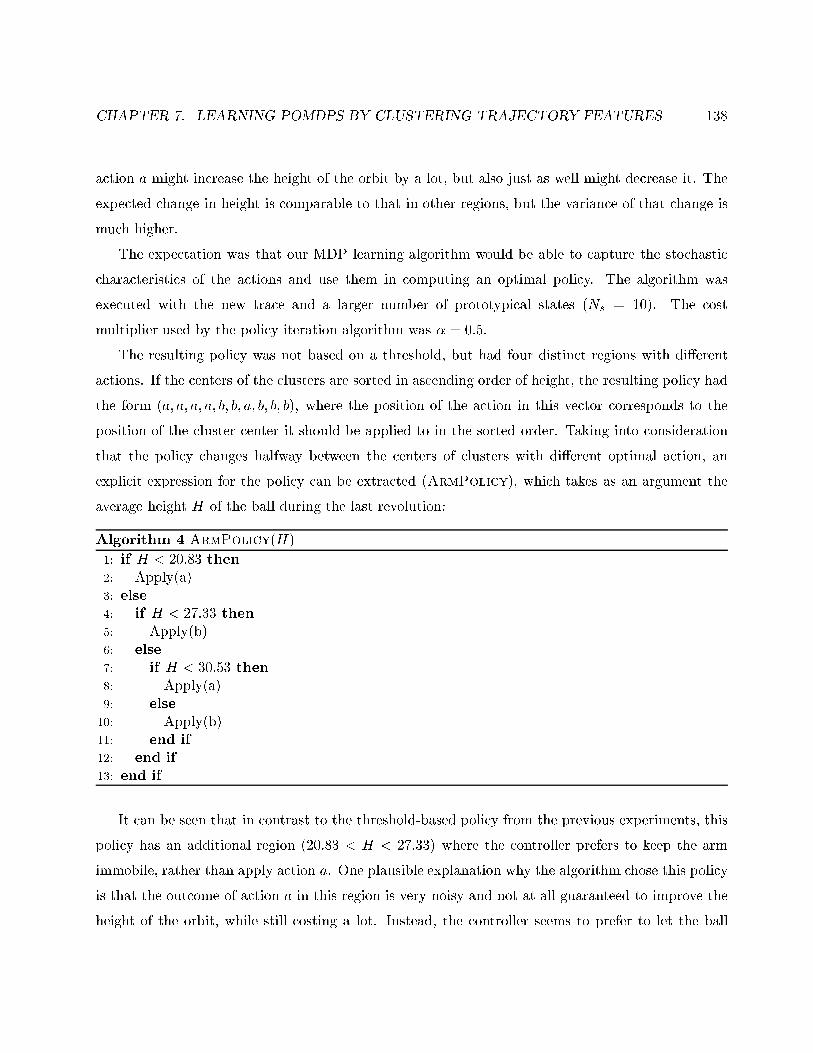
CHAPTER 7. LEARNING POMDPS BY CLUSTERING TRAJECTORY FEATURES 138
action a might increase the height of the orbit by a lot, but also just as well might decrease it. The
expected change in height is comparable to that in other regions, but the variance of that change is
much higher.
The expectation was that our MDP learning algorithm would be able to capture the stochastic
characteristics of the actions and use them in computing an optimal policy. The algorithm was
executed with the new trace and a larger number of prototypical states (Ns = 10). The cost
multiplier used by the policy iteration algorithm was � = 0:5.
The resulting policy was not based on a threshold, but had four distinct regions with di�erent
actions. If the centers of the clusters are sorted in ascending order of height, the resulting policy had
the form (a; a; a; a; b; b; a; b; b; b), where the position of the action in this vector corresponds to the
position of the cluster center it should be applied to in the sorted order. Taking into consideration
that the policy changes halfway between the centers of clusters with di�erent optimal action, an
explicit expression for the policy can be extracted (ArmPolicy), which takes as an argument the
average height H of the ball during the last revolution:
Algorithm 4 ArmPolicy(H)
1: if H < 20:83 then2: Apply(a)3: else
4: if H < 27:33 then5: Apply(b)6: else
7: if H < 30:53 then8: Apply(a)9: else
10: Apply(b)11: end if
12: end if
13: end if
It can be seen that in contrast to the threshold-based policy from the previous experiments, this
policy has an additional region (20:83 < H < 27:33) where the controller prefers to keep the arm
immobile, rather than apply action a. One plausible explanation why the algorithm chose this policy
is that the outcome of action a in this region is very noisy and not at all guaranteed to improve the
height of the orbit, while still costing a lot. Instead, the controller seems to prefer to let the ball
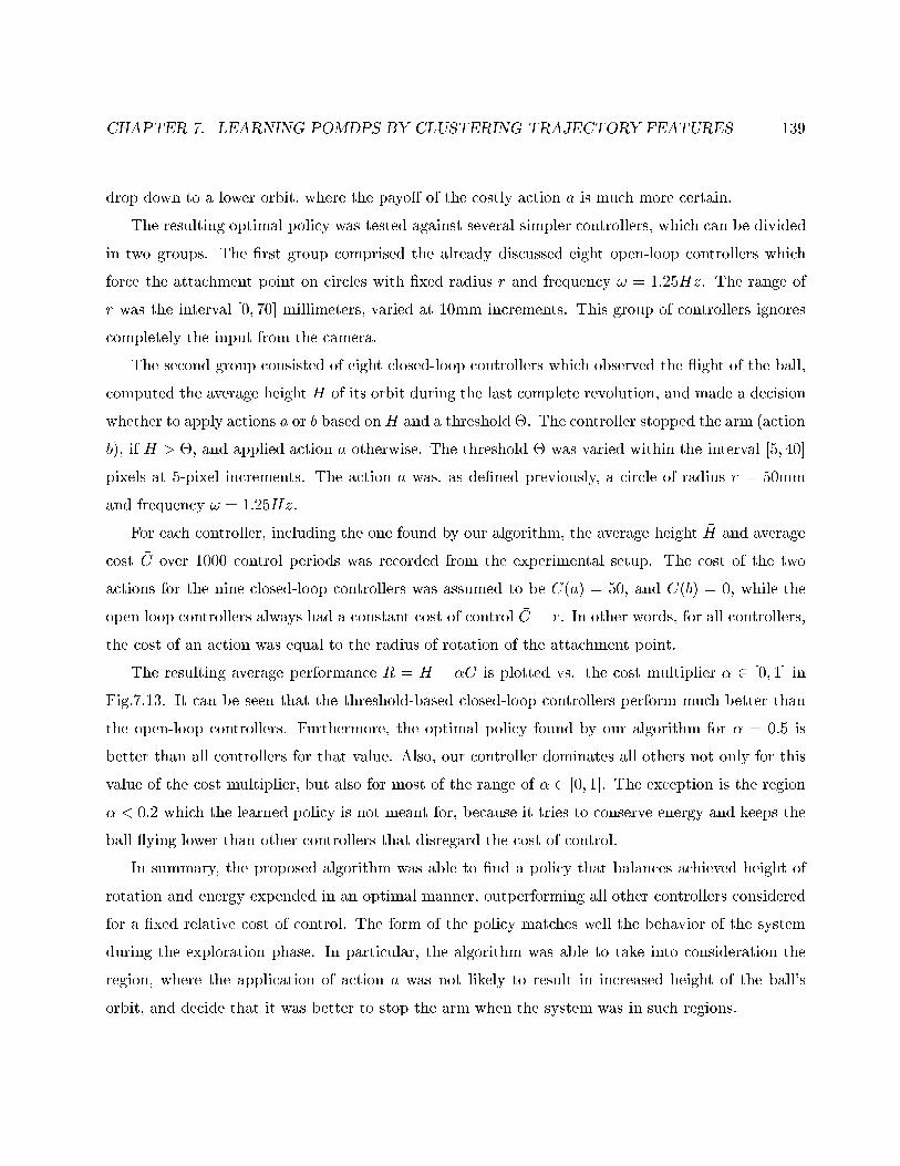
CHAPTER 7. LEARNING POMDPS BY CLUSTERING TRAJECTORY FEATURES 139
drop down to a lower orbit, where the payo� of the costly action a is much more certain.
The resulting optimal policy was tested against several simpler controllers, which can be divided
in two groups. The �rst group comprised the already discussed eight open-loop controllers which
force the attachment point on circles with �xed radius r and frequency ! = 1:25Hz. The range of
r was the interval [0; 70] millimeters, varied at 10mm increments. This group of controllers ignores
completely the input from the camera.
The second group consisted of eight closed-loop controllers which observed the ight of the ball,
computed the average height H of its orbit during the last complete revolution, and made a decision
whether to apply actions a or b based onH and a threshold �. The controller stopped the arm (action
b), if H > �, and applied action a otherwise. The threshold � was varied within the interval [5; 40]
pixels at 5-pixel increments. The action a was, as de�ned previously, a circle of radius r = 50mm
and frequency ! = 1:25Hz.
For each controller, including the one found by our algorithm, the average height �H and average
cost �C over 1000 control periods was recorded from the experimental setup. The cost of the two
actions for the nine closed-loop controllers was assumed to be C(a) = 50, and C(b) = 0, while the
open loop controllers always had a constant cost of control �C = r. In other words, for all controllers,
the cost of an action was equal to the radius of rotation of the attachment point.
The resulting average performance �R = �H � �C is plotted vs. the cost multiplier � 2 [0; 1] in
Fig.7.13. It can be seen that the threshold-based closed-loop controllers perform much better than
the open-loop controllers. Furthermore, the optimal policy found by our algorithm for � = 0:5 is
better than all controllers for that value. Also, our controller dominates all others not only for this
value of the cost multiplier, but also for most of the range of � 2 [0; 1]. The exception is the region
� < 0:2 which the learned policy is not meant for, because it tries to conserve energy and keeps the
ball ying lower than other controllers that disregard the cost of control.
In summary, the proposed algorithm was able to �nd a policy that balances achieved height of
rotation and energy expended in an optimal manner, outperforming all other controllers considered
for a �xed relative cost of control. The form of the policy matches well the behavior of the system
during the exploration phase. In particular, the algorithm was able to take into consideration the
region, where the application of action a was not likely to result in increased height of the ball's
orbit, and decide that it was better to stop the arm when the system was in such regions.
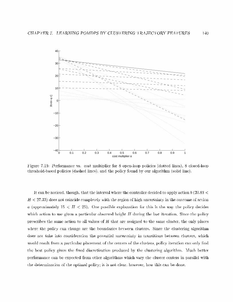
CHAPTER 7. LEARNING POMDPS BY CLUSTERING TRAJECTORY FEATURES 140
0 0.1 0.2 0.3 0.4 0.5 0.6 0.7 0.8 0.9 1−40
−30
−20
−10
0
10
20
30
40
cost multiplier α
R=
H−
α C
Figure 7.13: Performance vs. cost multiplier for 8 open-loop policies (dotted lines), 8 closed-loopthreshold-based policies (dashed lines), and the policy found by our algorithm (solid line).
It can be noticed, though, that the interval where the controller decided to apply action b (20:83 <
H < 27:33) does not coincide completely with the region of high uncertainty in the outcome of action
a (approximately 15 < H < 25). One possible explanation for this is the way the policy decides
which action to use given a particular observed height H during the last iteration. Since the policy
prescribes the same action to all values of H that are assigned to the same cluster, the only places
where the policy can change are the boundaries between clusters. Since the clustering algorithm
does not take into consideration the potential uncertainty in transitions between clusters, which
would result from a particular placement of the centers of the clusters, policy iteration can only �nd
the best policy given the �xed discretization produced by the clustering algorithm. Much better
performance can be expected from other algorithms which vary the cluster centers in parallel with
the determination of the optimal policy; it is not clear, however, how this can be done.
CHAPTER 7. LEARNING POMDPS BY CLUSTERING TRAJECTORY FEATURES 141
Another de�ciency of our algorithm is that the current scheme of de�ning states by means of
clustering before the policy is optimized matches the distribution of cluster states to the distribution
of data in the exploration policy. In contrast, at the time of execution, the controller would be helped
most if the distribution of the de�ned cluster states match the distribution of orbit height under the
optimal policy. However, the optimal policy itself cannot be found without �rst de�ning cluster
states. A solution to this problem is the one used in these experiments: construct an exploration
policy, which samples most densely the regions, where the optimal policy is likely to spend most of it
time. A better solution, again, would be to develop algorithms which ground clusters into continuous
states in parallel with the determination of the optimal policy.
In this chapter, the state merging approach was extended to a di�erent robotic application
| visual servo-control of manipulation. While the sensors used and the dynamics of the system
were very di�erent from the mobile robot localization problem explored in the previous chapter, an
algorithm based on the state-merging approach was still able to produce satisfactory solutions. This
is an indication that the proposed approach is not domain speci�c, but can be expected to perform
well on a variety of robotic tasks.
Chapter 8
Conclusions and Future Research
The main idea of this thesis is that probabilistic models for robot control can be learned successfully
by identifying which groups of states should be merged together in a single aggregated discrete state,
based on matching delayed sequences of percepts obtained from the execution of an appropriate
exploration policy. That this method succeeds should be no surprise, since the most successful
algorithms for linear system identi�cation are based on exactly the same idea, which so far has been
con�ned mainly to the �eld of control engineering. Consequently, the main contribution of this thesis
is in proposing algorithms which apply this idea to the problem of learning probabilistic models with
discrete state.
Certainly, there are critical di�erences between the sets of ordinary di�erential equations used
in control engineering, and the graphical probabilistic models used in reasoning and planning under
uncertainty. While the former have continuous state and control spaces and are mostly linear, the
latter usually have discrete states and actions and can represent arbitrary non-linear dependencies
and noise distributions. These di�erences require novel algorithmic solutions for implementing the
same basic idea. While most subspace system identi�cation methods in control engineering apply
Singular Value Decomposition on the sets of trajectory segments, the algorithms proposed in this
thesis apply clustering algorithms either directly on these trajectories, or on similarity matrices
derived from them. Even though the algorithmic solutions are di�erent, it should be recognized that
the proposed methods actually implement an approach long known and successfully used in control
engineering.
The algorithms proposed in this thesis are also contributions in terms of extending established
142
CHAPTER 8. CONCLUSIONS AND FUTURE RESEARCH 143
frameworks for reasoning and planning in autonomous systems in new directions. The SMTC algo-
rithm can be viewed as a means of enlarging the class of robots, for which probabilistic models can
be learned from data. Algorithms for learning probabilistic models in the form of global occupancy
grids have been known for robots which have fairly precise odometry and a full ring of proximity
sensors, but are generally not applicable to simpler robots without built-in odometry and a couple of
proximity sensors. The SMTC algorithm proposed in Chapter 5 is a means to extend probabilistic
robotics to such simpler and less expensive robots.
The same algorithm can also be considered to be an alternative, probabilistic implementation of
the topological layer of the Spatial Semantic Hierarchy. Instead of learning FSA and thus ignoring
the inherent uncertainty in perception and control, the topological layer can be represented by a
POMDP model which fully retains information about this uncertainty.
The proposed approach is also much more general than that of learning geometrical probabilistic
models such as global occupancy grids, as demonstrated by using it on two very di�erent robotic
tasks: mobile robot localization and visual servo-control of manipulation. It can be expected that it
could also be applied to many other control problems in robotics.
It should be noted, however, that this approach cannot be expected to perform well on all hard
control problems in robotics. The process of merging states is inherently a form of abstraction, and is
always accompanied by ignoring distinctions between the states that are merged. It is essential that
this abstraction do not eliminate important aspects of the dynamics of the system, which determine
the future evolution of this state. It is also essential that a good control policy be representable
in terms of the abstracted states. Both systems considered in this thesis �t these requirements. A
long enough sequence of discrete-valued compass readings is suÆcient for localization of a mobile
robot along the outer perimeter of its workspace, and the learned probabilistic model is capable
of encoding and recognizing all such sequences. If another control task requires full knowledge of
the continuous coordinates of the robot in con�guration space, a POMDP model learned by state
merging is not likely to succeed. Similarly, the visual servo-control task considered has dynamics that
can be approximated successfully in the quantized state space of orbit heights, and correspondingly,
a good control policy can be de�ned in terms of the quantized states. It is certain, however, that for
a system with such complicated and possibly chaotic continuous dynamics, many other tasks exist
which would require full and precise knowledge of the true continuous system state at all times.
These arguments delineate the class of problems that the state-merging approach to learning
CHAPTER 8. CONCLUSIONS AND FUTURE RESEARCH 144
POMDP models is suitable for. The restriction on actions to a small discrete set makes the approach
suitable for problems, where bang-bang control is suÆcient. This includes tasks such as the swing-
up pendulum (Doya, 1996; Doya, 1997), pole balancing (Jervis & Fallside, 1992), and the Acrobot
(Spong, 1995), as well as many other tasks that are isomorphic to them.
The algorithms proposed in this thesis make several restrictive assumptions which can possibly
be relaxed in future work. The most important assumption is that there is a single exploration
stage, during which an exploration trace is collected, and a single learning stage, during which the
probabilistic model is learned. In contrast, living organisms interleave smoothly exploration, learning,
and exploitation of the learned models. While it is not practical to re-learn the model after each new
percept is observed, it might be possible to alternate between several exploration and learning stages.
Of special interest are the composability of probabilistic models, which allows several sub-models to
be learned separately and then combined, and the Bayesian formulation of learning in probabilistic
models, where a previously learned model can serve as a prior in a posterior estimation scheme.
This scenario includes the important case when a preliminary map of the environment is available
(possibly only partial and/or imprecise). In such a case, this map can be used for localization
by means of belief tracking, which would identify states that are already represented in the map.
If localization does not succeed, this would mean that the robot is visiting new states, in which
case equivalence between pairs of them can be established by comparing trajectories, as described
in the previous chapters. Incorporating newly-identi�ed states into the original model (map) is
straightforward, since probabilistic models are easily composable. It is also known how to re�ne
the probabilities in such a model from subsequent observations | Baum-Welch has been shown
to work well for such tasks (Koenig & Simmons, 1996). Thus, learning the structure and initial
probabilities of a POMDP model by means of a state-merging algorithm such as SMTC does not
preclude the subsequent use of an iterative-adjustment algorithm such as Baum-Welch for the purpose
of improving the estimates of the probabilities in the model.
Interleaving exploration and learning might also solve another problem arising from the assump-
tions used in this thesis. That problem is the reliance on a single exploration policy which is expected
to sample the behavior of the system completely enough so that a model can be extracted from the
execution trace. As noted in Chapter 6, the only known method to cover completely the workspace
of a mobile robot without using some intermediate internal representation of that environment is to
perform random actions, which, in addition to being provably complete only in certain cases, takes
CHAPTER 8. CONCLUSIONS AND FUTURE RESEARCH 145
a very long time and usually produces incomplete and uneven coverage when the exploration stage
is limited to a short period. It is conceivable that a learned intermediate probabilistic model could
be used for planning the exploration process, much like partial global occupancy grids are used to
direct a mobile robot to unexplored portions of its workspace (Thrun et al., 1998a).
Another shortcoming of the proposed algorithms is that their policy optimization routines use
a �xed quantization of the state space and never reconsider it. As seen in Chapter 7, the quanti-
zation of the state space takes into consideration only the distribution of states visited during the
exploration stage, but ignores completely the transitions that took place during that stage. Since the
determination of the optimal policy is indirectly based on these transitions by means of the estimates
of transition probabilities between clusters, it might be expected that an algorithm which interleaves
quantization and policy improvement would perform better than one using a predetermined quan-
tization. Even more generally, all three stages | exploration, learning, and planning | can be
interleaved, merging states in a manner that would improve the control policy, while simultaneously
collecting new data that improves and extends the model.
Another direction of future research is to address the related problem of aggregating continuous
controls into discrete actions. The algorithms in this thesis used a manually selected set of actions
based on general understanding of the behavior of the controlled system. Even though there is
a similarity to the problem of abstracting states, as far as the process of �nding autonomously
appropriate discrete actions involves abstracting continuous variables into discrete ones, still that
process is very di�erent as well. For example, �nding discrete actions has no aliasing e�ects associated
with it, but, on the other hand, it is not clear how a space of actions could be \covered" by a
quantization scheme and what the meaning of such coverage would be. Furthermore, it is not clear
how two quantization schemes | one for states and another one for actions | could interact in order
to produce a tractable probabilistic model that is useful for planning and optimal control.
In terms of future applications of the proposed algorithms, several possibilities can readily be
identi�ed. The mobile robot localization method can be extended to explore parts of its workspace
other than its outer perimeter, by following other actions along with wall following. For example,
the robot can turn at straight angles from the wall and move along a straight line until it meets
another wall. This is likely to result in discovery of shorter routes to the goal state. Furthermore,
the method can be extended to handle workspaces with obstacles detached from the outer perimeter.
Such obstacles can be explored analogously to the case of exploring the inner perimeter, and a
CHAPTER 8. CONCLUSIONS AND FUTURE RESEARCH 146
separate probabilistic model can be learned for each obstacle. Planning in such workspaces then can
be implemented on a combined model consisting of several individual circular models connected by
several traverses.
The method for visual servo-control of manipulation can be extended for other tasks too. As
noted, most cranes have con�gurations similar to the experimental arm, and problems such as anti-
sway crane control when moving loads from point to point can be addressed by a modi�cation of
the proposed algorithm. Furthermore, the arm can be used for juggling tasks such as the Japanese
game of Kendama, where the ball is attached to the arm by a cord, instead of a rigid link, and
the objective is to move the arm in such a way that the ball lands in a basket attached to the arm
(Miyamoto et al., 1996). It can be seen that if our experimental arm is rotated 90o degrees around
the x-axis, so that the �rst and second actuated links now move in the xz-plane, the arm would be
able to implement the whipping motion necessary to land the ball in a basket attached to the arm.
In conclusion, this thesis proposed several algorithms for learning representations of dynamical
systems with non-linear dynamics and hidden state in the form of partially observable Markov
decision process (POMDP) models, and demonstrated how they can be applied to several robotic
tasks. Unlike most traditional methods for learning probabilistic models from data, the proposed
algorithms implement an approach characteristic of the dominant methods in the �eld of system
identi�cation. Much like in these methods, the establishment of similarity or equivalence between the
hidden states that might have been visited by the system at separate moments in time is implemented
by means of comparing trajectories of past and future percepts for these moments. However, since the
dynamics of a system has a very di�erent representation in a probabilistic model, novel algorithmic
solutions were proposed for comparing trajectories.
Apart from comparing the performance of the proposed algorithms to that of traditional methods
in simulation, the algorithms were also applied to two robots built in the course of thesis research: a
di�erential-drive mobile robot with a minimal number of proximity sensors, which has to localize itself
along the perimeter of its workspace, and an under-actuated arm observed from an non-calibrated
camera, which has to rotate a ying ball attached to it so as to maintain maximal height of rotation
with minimal energy expenditure. The application of the proposed algorithms to these two very
di�erent tasks resulted in better performance in comparison to alternative solutions, which suggests
that the algorithms might perform well on a wide variety of other robotic tasks. Still, the proposed
algorithmic solutions impose restrictions on the type of tasks that can be addressed by this approach,

CHAPTER 8. CONCLUSIONS AND FUTURE RESEARCH 147
and a number of directions were discussed for extending them to an even wider class of robotic
applications.
Appendix A
Derivation of the Equations of Motion
of the Arm
The chosen parametrization of the Cartesian coordinates (x; y; z) of the ball in terms of spherical
coordinates is:
x = r cos!t+ l sin � cos�
y = r sin!t+ l sin�
z = �l cos � cos�
In Lagrangian mechanics, the equations of motion are written in the following general form:
d
dt
�@L
@ _qi
�=
@L
@qi;
where L is the Lagrangian of the system, and qi are generalized coordinates. In our case, q1 = �
and q2 = �. The Lagrangian itself is the di�erence between the kinetic energy T of the system and
its potential energy U :
L = T � U
If we assume that the bob of the pendulum is a point with mass m, and the links have no mass,
the full kinetic energy is
148
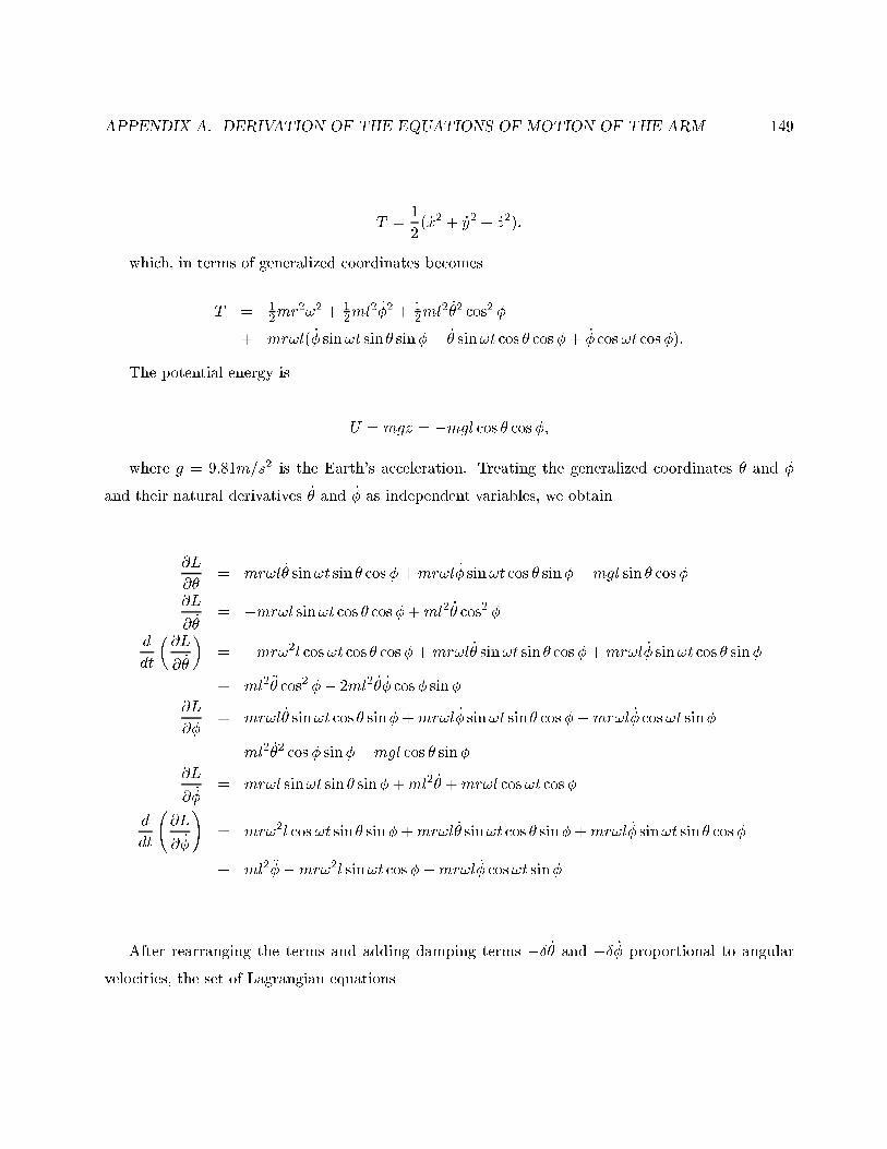
APPENDIX A. DERIVATION OF THE EQUATIONS OF MOTION OF THE ARM 149
T =1
2( _x2 + _y2 + _z2);
which, in terms of generalized coordinates becomes
T = 12mr2!2 + 1
2ml2 _�2 + 1
2ml2 _�2 cos2 �
+ mr!l( _� sin!t sin � sin�� _� sin!t cos � cos�+ _� cos!t cos�):
The potential energy is
U = mgz = �mgl cos � cos�;
where g = 9:81m=s2 is the Earth's acceleration. Treating the generalized coordinates � and �
and their natural derivatives _� and _� as independent variables, we obtain
@L
@�= mr!l _� sin!t sin � cos�+mr!l _� sin!t cos � sin��mgl sin � cos�
@L
@ _�= �mr!l sin!t cos � cos�+ml2 _� cos2 �
d
dt
�@L
@ _�
�= �mr!2l cos!t cos � cos�+mr!l _� sin!t sin � cos�+mr!l _� sin!t cos � sin�
+ ml2�� cos2 �� 2ml2 _� _� cos� sin�
@L
@�= mr!l _� sin!t cos � sin�+mr!l _� sin!t sin � cos��mr!l _� cos!t sin�
� ml2 _�2 cos� sin��mgl cos � sin�
@L
@ _�= mr!l sin!t sin � sin�+ml2 _� +mr!l cos!t cos�
d
dt
@L
@ _�
!= mr!2l cos!t sin � sin�+mr!l _� sin!t cos � sin�+mr!l _� sin!t sin � cos�
+ ml2 ���mr!2l sin!t cos��mr!l _� cos!t sin�
After rearranging the terms and adding damping terms �Æ _� and �Æ _� proportional to angular
velocities, the set of Lagrangian equations

APPENDIX A. DERIVATION OF THE EQUATIONS OF MOTION OF THE ARM 150
d
dt
�@L
@ _�
�=@L
@�
d
dt
@L
@ _�
!=@L
@�
can be expressed in canonical form as
�� = 2 _� _� tan�+r!2
l
cos!t cos �
cos��g
l
sin � cos �
cos2 �� Æ _�
�� = � _�2 cos� sin�� r!2[cos!t sin � sin�� sin!t cos�]�g
lcos � sin�� Æ _�:
Bibliography
Akulenko, L. D. (2000a). Control of the relative motions of a pendulum on a rotating base. Journal
of Applied Mathematics and Mechanics, 64, 197{208.
Akulenko, L. D. (2000b). Quasi-steady rotatory-vibratory motions of a two-mass system with a
vertically vibrating base. Journal of Applied Mathematics and Mechanics, 64, 51{60.
Alcal�a, R., Casillas, J., Cord�on, O., Herrera, J., & Zwir, S. (1999). Techniques for learning and
tuning fuzzy rule-based systems for linguistic modeling and their application. In C. Leondes (Ed.),
Knowledge engineering: Systems, techniques and applications. Academic Press.
Aston, P. J. (1999). Bifurcations of the horizontally forced spherical pendulum. Computational
Methods in Applied Mechanics and Engineering, 170, 343{353.
Barto, A. G. (1993). Arti�cial intelligence, neural networks, and control. In G. A. Bekey and K. Y.
Goldberg (Eds.), Neural networks in robotics. Kluwer Academic Press.
Baxter, J., & Bartlett, P. L. (2000). Reinforcement learning in POMDP's via direct gradient as-
cent. Proc. 17th International Conf. on Machine Learning (pp. 41{48). Morgan Kaufmann, San
Francisco, CA.
Bertsekas, D. P., & Casta~non, D. A. (1989). Adaptive aggregation methods for in�nite horizon
dynamic programming. IEEE Transactions on Automatic Control, 34, 589{598.
Bertsekas, D. P., & Tsitsiklis, J. N. (1989). Parallel and distributed computation. Englewood Cli�s,
NJ: Prentice-Hall.
Best, D. J., & Fisher, N. I. (1979). EÆcient simulation of the von Mises distribution. Applied
Statistics, 28, 152{157.
151
BIBLIOGRAPHY 152
Binder, J., Murphy, K., & Russell, S. (1997). Space-eÆcient inference in dynamic probabilistic
networks. Proceedings of the 15th International Joint Conference on Arti�cial Intelligence (IJCAI-
97) (pp. 1292{1296). San Francisco: Morgan Kaufmann Publishers.
Boyan, J. A., & Moore, A. W. (1995). Generalization in reinforcement learning: Safely approxi-
mating the value function. Advances in Neural Information Processing Systems 7 (pp. 369{376).
Cambridge, MA: The MIT Press.
Brooks, R. A. (1985). A layered intelligent control system for a mobile robot. Third International
Symposium of Robotics Research (pp. 1{8). Gouvieux, France.
Brooks, R. A. (1991). Intelligence without representation. Arti�cial Intelligence, 47, 139{159.
Brown, C., Durrant-Whyte, H., Leonard, J., & Rao, B. (1989). Centralized and decentralized kalman
�lter techniques for tracking, navigation, and control. Image Understanding Workshop (Palo Alto,
CA). San Mateo, CA: Morgan Kaufmann.
Bryant, P. J. (1993). Breakdown to chaotic motion of a forced, damped, spherical pendulum. Physica
D, 64, 324{339.
Buhmann, J. M., & Hofmann, T. (1995). Pairwise data clustering by deterministic anneal-
ingTechnical Report IAI-TR-95-7). University of Bonn, Department of Computer Science.
Butler, Z. (1998). CCR : A complete algorithm for contact-sensor based coverage of rectilinear
environments (Technical Report CMU-RI-TR-98-27). The Robotics Institute, Carnegie Mellon
University.
Cassandra, A. R., Kaelbling, L. P., & Kurien, J. A. (1996). Acting under uncertainty: Discrete
Bayesian models for mobile robot navigation. Proceedings of IEEE/RSJ International Conference
on Intelligent Robots and Systems.
Chatelin, F., & Miranker, W. L. (1982). Acceleration by aggregation of successive approximation
methods. Linear Algebra and its Applications, 43, 17{47.
Choset, H. (2001). Coverage for robotics | a survey of recent results. Annals of Mathematics and
Arti�cial Intelligence, 31, 113{126.
BIBLIOGRAPHY 153
Chrisman, L. (1992). Reinforcement learning with perceptual aliasing: The perceptual distinctions
approach. Proceedings of the 10th National Conference on Arti�cial Intelligence (pp. 183{188).
San Jose, CA: MIT Press.
Cooper, G. (1990). Computational complexity of probabilistic inference using Bayesian belief net-
works (Research note). SIAM Journal on Computing, 42, 393{405.
Cormen, T. H., Leiserson, C. E., & Rivest, R. L. (1991). Introduction to algorithms. Cambridge,
Massachusetts: MIT Press/McGraw-Hill.
Craig, J. J. (1986). Introduction to robotics. mechanics & control. Addison-Wesley.
Crites, R. H., & Barto, A. G. (1996). Improving elevator performance using reinforcement learning.
Advances in Neural Information Processing Systems (pp. 1017{1023). The MIT Press.
Dean, T., Angluin, D., Basye, K., Engelson, S., Kaelbling, L., Kokkevis, E., & Maron, O. (1995).
Inferring �nite automata with stochastic output functions and an application to map learning.
Machine Learning, 18, 81.
Dean, T., & Kanazawa, K. (1989). A model for reasoning about persistence and causation. Compu-
tational Intelligence, 5, 142{150.
Dean, T. L., & Wellman, M. P. (1991). Planning and control. San Mateo, California: Morgan
Kaufmann.
DeMers, D., & Kreutz-Delgado, K. (1992). Learning global direct inverse kinematics. Advances in
Neural Information Processing Systems (pp. 589{595). Morgan Kaufmann Publishers, Inc.
Dempster, A. P., Laird, N. M., & Rubin, D. B. (1977). Maximum likelihood from incomplete data
via the EM algorithm (with discussion). Journal of the Royal Statistical Society series B, 39, 1{38.
Doya, K. (1996). Temporal di�erence learning in continuous time and space. Advances in Neural
Information Processing Systems (pp. 1073{1079). The MIT Press.
Doya, K. (1997). EÆcient nonlinear control with actor-tutor architecture. Advances in Neural
Information Processing Systems (p. 1012). The MIT Press.
BIBLIOGRAPHY 154
Driankov, D., Hellendoorn, H., & Reinfrank, M. (1993). An introduction to fuzzy control. Springer
Verlag, Heidelberg.
Duda, R., & Hart, P. (1973). Pattern recognition and scene analysis. John Wiley and Sons.
Elkan, C. (1994). The paradoxical success of fuzzy logic. IEEE Expert August 1994.
Fahlman, S. E. (1989). Faster-learning variations on back-propagation: an empirical study. Proceed-
ings of the 1988 Connectionist Models Summer School, Pittsburg (pp. 38{51). San Mateo, CA:
Morgan Kaufmann.
Fikes, R. E., & Nilsson, N. J. (1971). STRIPS: A new approach to the application of theorem proving
to problem solving. Proceedings of the 2nd International Joint Conference on Arti�cial Intelligence
(pp. 608{620). London, UK: William Kaufmann.
Franklin, G. F., Powell, J. D., & Emami-Naeini, A. (1987). Feedback control of dynamic systems.
Addison Wesley.
Fu�cik, S. (1980). Solvability of nonlinear equations and boundary value problems. Dordrecht: Reidel.
Gat, E. (1998). Three-layer architectures. In D. Kortenkamp, R. Bonasso and R. Murphy (Eds.),
Arti�cial intelligence and mobile robots, 195{210. Cambridge: MIT Press.
Ghahramani, Z. (1998). Learning dynamic Bayesian networks. Lecture Notes in Computer Science,
1387, 168{198.
Ghahramani, Z., & Jordan, M. I. (1997). Factorial hidden Markov models. Machine Learning, 29,
245{273.
Glasius, R., Komoda, A., & Gielen, S. C. A. M. (1995). Neural network dynamics for path planning
and obstacle avoidance. Neural Networks, 8, 125{133.
Goh, C. J. (1993). On the nonlinear optimal regulator problem. Automatica, 29, 751{756.
Gordon, G. J. (1996). Stable �tted reinforcement learning. Advances in Neural Information Process-
ing Systems (pp. 1052{1058). The MIT Press.
BIBLIOGRAPHY 155
Gorman, R. P., & Sejnowski, T. J. (1988). Analysis of hidden units in a layered network trained to
classify sonar targets. Neural Networks, 1, 75{89.
Greiner, R. (1999). The complexity of theory revision. Arti�cial Intelligence, 107, 175{217.
Harnad, S. (1990). The symbol grounding problem. Physica D, 42, 335{346.
Hashimoto, H., Kubota, T., Sato, N., & Harashima, F. (1992). Visual control of robotic manipulator
based on neural networks. IEEE Transaction on Industrial Electronics, 39, 490{496.
Heckerman, D., Geiger, D., & Chickering, D. M. (1995). Learning Bayesian networks: the combina-
tion of knowledge and statistical data. Machine Learning, 20, 197{243.
Heng, H., & Martienssen, W. (1992). Analysing the chaotic motion of a driven pendulum. Chaos,
Solitons, and Fractals, 2, 323{334.
Hert, S., Tiwari, S., & Lumelsky, V. (1996). A terrain-covering algorithm for an auv. Journal of
Autonomous Robots, 3, 91{119.
Hertz, J., Krogh, A., & Palmer, R. G. (1991). An introduction to the theory of neural computation.
Lecture Notes Volume I. Addison Wesley.
Honkela, A. (2001). Nonlinear switching state-space models. Master's thesis, Helsinki University of
Technology, Espoo, Finland.
Hunter, N. F. (1997). State analysis of nonlinear systems using local canonical variate analysis.
Proceedings of the Thirtieth Hawaii International Conference on System Sciences (pp. 491{500).
Los Alamitos, CA, USA: IEEE Comput. Soc. Press.
Hutchinson, S., Hager, G., & Corke, P. (1996). A tutorial on visual servo control. IEEE Trans.
Robot. Automat., 12, 651{670.
Jaakkola, T., Jordan, M. I., & Singh, S. P. (1994). Convergence of stochastic iterative dynamic
programming algorithms. Advances in Neural Information Processing Systems (pp. 703{710).
Morgan Kaufmann Publishers, Inc.
Jervis, T. T., & Fallside, F. (1992). Pole balancing on a real rig using a reinforcement learning
controller (Technical Report CUED/F-INFENG/TR. 115). Cambridge University, UK.
BIBLIOGRAPHY 156
Jordan, M. I., & Rumelhart, D. E. (1992). Forward models: Supervised learning with a distal teacher.
Cognitive Science, 16, 307{354.
Kaelbling, L. P., Littman, M. L., & Cassandra, A. R. (1996). Planning and acting in partially
observable stochastic domains (Technical Report CS-96-08). Brown University, Providence, RI.
Kanazawa, K., Koller, D., & Russell, S. (1995). Stochastic simulation algorithms for dynamic prob-
abilistic networks. Proceedings of the 11th Conference on Uncertainty in Arti�cial Intelligence
(UAI'95) (pp. 346{351). San Francisco, CA, USA: Morgan Kaufmann Publishers.
Kelly, A. (2000). Some useful results for closed-form propagation of error in vehicle odome-
tryTechnical Report CMU-RI-TR-00-20). Carnegie Mellon University: The Robotics Institute.
Klingspor, V., Morik, K. J., & Rieger, A. D. (1996). Learning concepts from sensor data of a mobile
robot. Machine Learning, 23, 305{332.
Koenig, S., & Simmons, R. (1996). Unsupervised learning of probabilistic models for robot navigation.
Proceedings of the IEEE International. Conference on Robotics and Automation.
Koenig, S., & Simmons, R. (1998). Xavier: a robot navigation architecture based on partially
observable Markov decision process models. In D. Kortenkamp, R. Bonasso and R. Murphy (Eds.),
Arti�cial intelligence and mobile robots, 91{122. Cambridge: MIT Press.
Kortenkamp, D., Bonasso, R., & Murphy, R. (1998). Arti�cial intelligence and mobile robots: Case
studies of successful robot systems. Cambridge, MA: MIT Press.
Koza, J. R. (1994). Evolution of a subsumption architecture that performs a wall following task
for an autonomous mobile robot via genetic programming. In T. Petsche (Ed.), Computational
learning theory and natural learning systems, vol. 2, 321{346. Cambridge, MA, USA: MIT Press.
Kr�ose, B. J. A., & Eecen, M. (1994). A self-organizing representation of sensor space for mobile
robot navigation. In Proceedings of the ieee/rsj/gi international conference on intelligent robots
and systems, 9{14. IEEE.
Kr�ose, B. J. A., & van Dam, J. W. M. (1992). Adaptive state space quantisation: adding and
removing neurons. Arti�cial Neural Networks (pp. 619{622). Elsevier Science Publishers B.V.
BIBLIOGRAPHY 157
Kuipers, B., & Byun, Y.-T. (1991). A robot exploration and mapping strategy based on a semantic
hierachy of spatial representations. Robotics and Autonomous Systems, 8, 46{63.
Kuipers, B. J., & Levitt, T. S. (1988). Mavigation and mapping large-scale space. AI Magazine, 9,
25{43.
Laird, J. E., Newell, A., & Rosenbloom, P. S. (1987). SOAR: an architecture for general intelligence.
Arti�cial Intelligence, 33, 1{64.
Laird, J. E., & Rosenbloom, P. S. (1990). Integrating, execution, planning, and learning in Soar for
external environments. Proceedings of the 8th National Conference on Arti�cial Intelligence (pp.
1022{1029). Hynes Convention Centre: MIT Press.
Lakshmirvarahaan, S. (1981). Learning algorithms theory and applications. New York: Springer.
Larimore, W. E. (1990). Canonical variate analysis in identi�cation, �letering, and adaptive control.
Proceedings of the 29th Conference on Decision and Control, Hawaii (pp. 596{604.).
Latombe, J.-C. (1991). Robot motion planning. Boston: Boston: Kluwer Academic Publishers.
Law, D., & Miikkulainen, R. (1994). Grounding robotic control with genetic neural networks (Tech-
nical Report AI94-223). Department of Computer Sciences, The University of Texas at Austin.
Leung, M.-Y., Blaisdell, B., Burge, C., & Karlin, S. (1991). An eÆcient algorithm for identifying
matches with errors in multiple long molecular sequences. Journal of Molecular Biology, 221,
1367{78.
Lin, L.-J., & Mitchell, T. M. (1992). Memory approaches to reinforcement learning in non-markovian
domainsTechnical Report CS-92-138). Carnegie Mellon University, School of Computer Science.
Littman, M. L., Dean, T. L., & Kaelbling, L. P. (1995). On the complexity of solving Markov decision
problems. Proceedings of the Eleventh Annual Conference on Uncertainty in Arti�cial Intelligence
(UAI{95) (pp. 394{402). Montreal, Qu�ebec, Canada.
Liu, K., & Lewis, F. L. (1992). Application of robust control techniques to a mobile robot system.
Journal of Robotic Systems, 9, 893{913.
BIBLIOGRAPHY 158
Lu, F., & Milios, E. (1997). Globally consistent range scan alignment for environment mapping.
Autonomous Robots, 4, 333{349.
Mahadevan, S., & Connell, J. (1992). Automatic programming of behavior-based robots using rein-
forcement learning. Arti�cial Intelligence, 55, 311{365.
Mardia, K. V., & Jupp, P. E. (2000). Directional statistics. New York: Wiley.
Marsden, J., & Ratiu, T. (1998). Introduction to mechanics and symmetry, second edition. Springer
Verlag.
Mataric, M. J. (1990). A distributed model for mobile robot environment-learning and navigation
(Technical Report AI-TR 1228). MIT Arti�cial Intelligence Laboratory.
Matari�c, M. J. (1992). Integration of representation into goal-driven behavior-based robots. IEEE
Trans. Robotics and Automation, 8, 304{312.
McCallum, R. A. (1995). Instance-based state identi�cation for reinforcement learning. Advances in
Neural Information Processing Systems (pp. 377{384). The MIT Press.
Meuleau, N., Peshkin, L., Kim, K.-E., & Kaelbling, L. P. (1999). Learning �nite-state controllers for
partially observable environments. Proceedings of the 15th Conference on Uncertainty in Arti�cial
Intelligence (UAI-99) (pp. 427{436). S.F., Cal.: Morgan Kaufmann Publishers.
Miles, J. (1984). Resonant motion of spherical pendulum. Physica D, 11, 309{323.
Miles, J. (1993). Damped spherical pendulum. Journal of Sound and Vibrations, 140, 327{330.
Mitchell, T. M. (1978). Version spaces: An approach to concept learning (Technical Report HPP-
79-2). Stanford University, Palo Alto, CA.
Mitchell, T. M. (1997). Machine learning. McGraw-Hill.
Miyamoto, H., Schaal, S., Gandolfo, F., Gomi, H., Koike, Y., Osu, R., Nakano, E., Wada, Y., &
Kawato, M. (1996). A kendama learning robot based on bi-directional theory. Neural Networks,
9, 1281{1302.
BIBLIOGRAPHY 159
Moore, A. W., & Atkeson, C. G. (1992). Memory-based function approximators for learning control
(Technical Report). MIT, MIT Arti�cial Intelligence Laboratory, Cambridge, MA 02139.
Moravec, H. (1999). Robot: Mere machine to transcendent mind. Oxford: Oxford University Press.
Moravec, H. P. (1977). Visual mapping by a robot rover. Proc. 5th Join International Conference
of Arti�cial Intelligence (pp. 598{600). Tokyo, Japan.
Mozer, M. C., & Bachrach, J. (1989). Discovering the structure of a reactive environment by ex-
ploration (Technical Report CU-CS-451-89). Dept. of Computer Science, University of Colorado,
Boulder.
Mozer, M. C., & Bachrach, J. (1991). Slug: A connectionist architecture for inferring the structure
of �nite-state environments. Machine Learning, 7, 139{160.
Munos, R., Baird, L., & Moore, A. (1999). Gradient descent approaches to neural-net based solutions
of the Hamilton-Jacobi-Bellman equation. International Joint Conference on Neural Networks.
Munos, R., & Moore, A. (1998). Barycentric interpolators for continuous space and time reinforce-
ment learning. Advances in Neural Information Processing Systems. Cambridge, MA: MIT Press.
Murray, R. (1995). Nonlinear control of mechanical systems: A lagrangian perspective. IFAC
Symposium on Nonlinear Control Systems Design (NOLCOS), (Tahoe City) (pp. 378{389).
Narendra, K., & Parthasarathy, K. (1990). Identi�cation and control of dynamical systems using
neural networks. IEEE Transactions on Neural Networks, 1, 4{27.
Nehmzow, U., & Smithers, T. (1992). Using motor actions for location recognition. Toward a Practice
of Autonomous Systems. Proc. First European Conf. on Arti�cial Life (pp. 96{104). Cambridge,
MA, USA: MIT Press.
Newell, A., & Simon, H. A. (1976). Computer science as empirical enquiry. Communications of the
ACM, 19, 113{126.
Ng, A. Y., & Jordan, M. (2000). PEGASUS: a policy search method for large MDPs and POMDPs.
Proceedings of the 2000 Conference on Uncertainty in Arti�cial Intelligence.
BIBLIOGRAPHY 160
Ngo, L., & Haddawy, P. (1995). Probabilistic logic programming and Bayesian networks. Lecture
Notes in Computer Science, 1023, 286.
Nomadic-Technologies (1997). Nomad 150: User's manual. Mountain View, CA.
Nourbakhsh, I. (1998). Dervish: an oÆce navigating robot. In D. Kortenkamp, R. Bonasso and
R. Murphy (Eds.), Arti�cial intelligence and mobile robots, 73{90. Cambridge: MIT Press.
Ormoneit, D., & Sen, S. (1999). Kernel-based reinforcement learning (Technical Report 1999-8).
Department of Statistics, Stanford University.
Overschee, P. V., &Moor, B. D. (1994). N4sid: Subspace algorithms for the identi�cation of combined
deterministic-stochastic systems. Automatica, 30, 75{93.
Parr, R., & Russell, S. (1995). Approximating optimal policies for partially observable stochastic
domains. Proceedings of the International Joint Conference on Arti�cial Intelligence.
Pearl, J. (1988). Probabilistic reasoning in intelligent systems: Networks of plausible inference. San
Mateo, California: Morgan Kaufmann.
Penberthy, J. S., & Weld, D. S. (1992). UCPOP: A sound, complete, partial order planner for ADL.
Proceedings of the 3rd International Conference on Principles of Knowledge Representation and
Reasoning (pp. 103{114). Cambridge, MA: Morgan Kaufmann.
Pierce, D., & Kuipers, B. (1994a). How an embedded agent can infer the structure of a continuous
world. ML/COLT94 Robot Learning Workshop, Rutgers University.
Pierce, D., & Kuipers, B. (1994b). Learning to explore and build maps. Proceedings of AAAI-94
(pp. 1264{1271).
Pierce, D., & Kuipers, B. (1997). Map learning with uninterpreted sensors and e�ectors. Arti�cial
Intelligence Journal, 92, 169{227.
Pomerleau, D. A. (1993). Neural network perception for mobile robot guidance. Dordrecht, The
Netherlands: Kluwer.
Press, W. H., Teukolsky, S. A., Vetterling, W. T., & Flannery, B. P. (1992). Numerical recipes in C,
2nd. edition. Cambridge University Press.
BIBLIOGRAPHY 161
Puterman, M. L. (1994). Markov decision processes|discrete stochastic dynamic programming. New
York, NY: John Wiley & Sons, Inc.
Rabiner, L. R., & Juang, B. H. (1986). An introduction to hidden Markov models. IEEE ASSP
Magazine, 4.
Rabiner, L. R., Juang, B.-H., Levinson, S. E., & Sondhi, M. M. (1985). Some properties of continuous
hidden Markov model representations. AT&T Technical Journal, 64, 1251{1270.
Roumeliotis, S., & Bekey, G. (2000). Collective localization: a distributed kalman �lter approach to
localization of groups of mobile robots. IEEE International Conference on Robotics and Automa-
tion.
Rumelhart, D. E., Hinton, G. E., & Williams, R. J. (1986). Learning internal representation by error
propagation. In D. E. Rumelhart and J. L. McClelland (Eds.), Parallel distributed processing:
Explorations in the microstructure of cognition, vol. 1, 318{362. Cambridge, MA: MIT Press.
Rumelhart, D. E., & McClelland, J. L. (1986). Parallel distributed processing: Explorations in the
microstructure of cognition. vols. I and II. Cambridge, MA: MIT Press.
Russell, S., Binder, J., & Koller, D. (1994). Adaptive probabilistic networksTechnical Report CSD-
94-824). University of California, Berkeley.
Russell, S. J., & Norvig, P. (1995). Arti�cial intelligence. A modern approach. Englewood Cli�s:
Prentice-Hall.
SaÆotti, A., & Wesley, L. P. (1996). Perception-based self-localization using fuzzy locations. In van
M. Lambalgen L. Dorst and F. Voorbraak (Eds.), Reasoning with uncertainty in robotics | procs.
of the international workshop, 368{385. Berlin, Germany: LNAI 1093, Springer.
Sauer, T. (1993). Time series prediction by using delay coordinate embedding. In A. S. Weigend
and N. A. Gershenfeld (Eds.), Time series prediction: Forecasting the future and understanding
the past, 175{193. Reading, MA: Addison Wesley.
Sauer, T., Yorke, J. A., & Casdagli, M. (1991). Embedology. J. Stat. Phys., 65, 579{616.
BIBLIOGRAPHY 162
Schoppers, M. J. (1987). Universal plans for reactive robots in unpredictable environments. Pro-
ceedings of the Tenth International Joint Conference on Arti�cial Intelligence (IJCAI-87) (pp.
1039{1046). Milan, Italy: Morgan Kaufmann publishers Inc.: San Mateo, CA, USA.
Shann, J., & Fu, H. C. (1995). A fuzzy neural network for rule acquiring on fuzzy control systems.
Fuzzy Sets and Systems, 71, 345{357.
Shatkay, H. (1998). Learning models for robot navigation (Technical Report CS-98-11). Brown
University, Department of Computer Science.
Shimojima, K., Hasegawa, Y., & Fukuda, T. (1995). Unsupervised/supervised learning for RBF-
fuzzy system. Advances in Fuzzy Logic, Neural Networks and Genetic Algorithms (pp. 127{147).
Berlin: Springer Verlag.
Simmons, R., & Koenig, S. (1995). Probabilistic robot navigation in partially observable environ-
ments. Proceedings of the International Joint Conference on Arti�cial Intelligence (pp. 1080{1087).
Sjoberg, J., Zhang, Q., Ljung, L., Benveniste, A., Delyon, B., Glorennec, P., Hjalmarsson, H., &
Juditsky, A. (1995). Nonlinear black-box modeling in system identi�cation: a uni�ed overview.
Automatica, 31, 1691{1724.
Slotine, J. J., & Lee, W. (1990). Applied non-linear control. Prentice-Hall.
Sondik, E. J. (1971). The optimal control of partially observable Markov decision processes. Doctoral
dissertation, Stanford University, Stanford, California.
Song, Y., & Grizzle, J. (1995). The extended Kalman �lter as a local asymptotic observer for
discrete-time nonlinear systems.
Spong, M. (1995). The swingup control problem for the acrobot. IEEE Control Systems Magazine,
Feb.
Stengel, R. (1994). Optimal control and estimation. New York: Dover.
Stolcke, A., & Omohundro, S. (1993). Hidden Markov Model induction by bayesian model merging.
Advances in Neural Information Processing Systems (pp. 11{18). Morgan Kaufmann, San Mateo,
CA.
BIBLIOGRAPHY 163
Sussman, G. J., & Wisdom, J. (2001). Structure and interpretation of classical mechanics. Cam-
bridge, Massachusetts: The MIT Press.
Sutton, R. S., & Barto, A. G. (1998). Reinforcement learning. Cambridge, Massachusetts: The MIT
Press.
Takens, F. (1980). Detecting strange attractors in turbulence. In D. A. Rand and L.-S. Young (Eds.),
Dynamical systems and turbulence (warwick 1980), vol. 898, 366{381. Berlin: Springer-Verlag.
Takens, F. (1985). On the numerical determination of the dimension of an attractor. In B. L. J.
Braaksma, H. W. Broer and F. Takens (Eds.), Dynamical systems and bifurcations, groningen
1984, vol. 1125 of Lecture Notes in Mathematics, 99{106. Berlin: Springer-Verlag.
Tesauro, G. (1992). Practical issues in temporal di�erence learning. Machine Learning, 8, 257{278.
Thrun, S. (2000). Probabilistic algorithms in robotics. AI Magazine, 21, 93{109.
Thrun, S., Buecken, A., Burgard, W., Fox, D., Froehlinghaus, T., Hennig, D., Hofmann, T., Krell,
M., & Schmidt, T. (1996). Map learning and high-speed navigation in RHINOTechnical Report
IAI-TR-96-3). University of Bonn, Department of Computer Science.
Thrun, S., Buecken, A., Burgard, W., Fox, D., Froehlinghaus, T., Hennig, D., Hofmann, T., Krell, M.,
& Schmidt, T. (1998a). Map learning and high-speed navigation in RHINO. In D. Kortenkamp,
R. Bonasso and R. Murphy (Eds.), Arti�cial intelligence and mobile robots, 21{52. Cambridge:
MIT Press.
Thrun, S., Burgard, W., & Fox, D. (1998b). A probabilistic approach to concurrent mapping and
localization for mobile robots. Machine Learning, 31, 29.
Thrun, S., Fox, D., & Burgard, W. (1998c). Probabilistic mapping of an environment by a mobile
robot. Proceedings of the IEEE International Conference on Robotics and Automation (ICRA-98)
(pp. 1546{1551). Piscataway: IEEE Computer Society.
Tritton, D. J. (1986). Ordered and chaotic motion of a forced sperical pendulum. European Journal
of Physics, 7, 162{169.
BIBLIOGRAPHY 164
Tsitsiklis, J. N., & van Roy, B. (1996). Feature-based methods for large scale dynamic programming.
Machine Learning, 22, 59{94.
Tunstel, E., Danny, H., Lippincott, T., & Jamshidi, M. (1997). Autonomous navigation using an
adaptive hierarchy of multiple fuzzy behaviors. Proc. of the IEEE Int. Sym. on Computational
Intelligence in Robotics and Automation. Monterey, CA.
Tversky, A., & Kahneman, D. (1982). Judgement under uncertainty: heuristics and biases. In
D. Kahneman, P. Slovic and A. Tversky (Eds.), Judgement under uncertainty: heuristics and
biases, chapter 1, 3{20. Cambridge: Cambridge University Press.
van der Smagt, P. P., Kr�ose, B. J. A., & Groen, F. C. A. (1992). A self-learning controller for
monocular grasping. In Proceedings of the 1992 ieee/rsj international conference on intelligent
robots and systems, 177{182. Raleigh, N. C.: IEEE.
van Turennout, P., Honderd, G., & van Schelven, L. (1992). Wall-following control of a mobile robot.
IEEE International Conference on Robotics and Automation (pp. 280{285).
Viberg, M., Wahlberg, B., & Ottersten, B. (1997). Analysis of state space system identi�cation
methods based on instrumental variables and subspace �tting. Automatica, 33, 1603{1616.
Wan, E. A. (1993). Time series prediction by using a connectionist network with internal delay lines.
In A. S. Weigend and N. A. Gershenfeld (Eds.), Time series prediction: Forecasting the future and
understanding the past;, 195{217. Reading, MA: Addison Wesley.
Watanabe, S., & Masahide, Y. (1992). An ultrasonic visual sensor for three-dimensional object
recognition using neural networks. IEEE Transactions on Robotics and Automation, 8, 36{55.
Watkins, C. J. (1989). Models of delayed reinforcement learning. Doctoral dissertation, Psychology
Department, Cambridge University, Cambridge, United Kingdom.
Welch, G., & Bishop, G. (1995). An introduction to the kalman �lter (Technical Report TR95-041).
University of North Carolina, Department of Computer Science.
Wiener, N. (1948). Cybernetics, or control and communication in the animal and the machine. New
York: John Wiley.
Wiener's classic book on cybernetics. Second edition with additions published in 1961.
BIBLIOGRAPHY 165
Williams, R. J. (1992). Simple statistical gradient-following algorithms for connectionist reinforce-
ment learning. Machine Learning, 8, 229{256.
Williams, R. J., & Zipser, D. (1989). A learning algorithm for continually running fully recurrent
neural networks. Neural Computation, In this volume.
Wrobel, S. (1994). Concept formation and knowledge revision. Dordrecht, Holland: Kluwer Academic
Publishers.
Yata, T., Kleeman, L., & Yuta, S. (1998). Wall following using angle information measured by a single
ultrasonic transducer. International Conference on Robotics and Automation (pp. 1590{1596).
Zalzala, A., & Morris, A. (1996). Neural networks for robotic control: Theory and applications. New
York: Ellis Horwood.
Zelinsky, A. (1991). Mobile robot map making using sonar. Journal of Robotic Systems, 8, 557{577.
Zelinsky, A. (1992). A mobile robot navigation exploration algorithm. IEEE Transactions of Robotics
and Automation, 8, 707{717.
Zhang, W., & Dietterich, T. G. (1996). High-performance job-shop scheduling with A time-delay
TD� network. Advances in Neural Information Processing Systems (pp. 1024{1030). The MIT
Press.