Embed Size (px)
Citation preview

SANDIA REPORTSAND2017-4401Unlimited ReleasePrinted April 2017
State estimation for wave energyconverters
Giorgio Bacelli and Ryan G. Coe
Prepared bySandia National LaboratoriesAlbuquerque, New Mexico 87185 and Livermore, California 94550
Sandia National Laboratories is a multi-mission laboratorymanaged and operated by National Technology and Engineering Solutions of Sandia, LLC.,a wholly owned subsidiary of Honeywell International, Inc.,for the U.S. Department of Energy’s National Nuclear Security Administrationunder contract DE-NA0003525.
Approved for public release; further dissemination unlimited.
Issued by Sandia National Laboratories, operated for the United States Department of Energyby National Technology and Engineering Solutions of Sandia, LLC..
NOTICE: This report was prepared as an account of work sponsored by an agency of the UnitedStates Government. Neither the United States Government, nor any agency thereof, nor anyof their employees, nor any of their contractors, subcontractors, or their employees, make anywarranty, express or implied, or assume any legal liability or responsibility for the accuracy,completeness, or usefulness of any information, apparatus, product, or process disclosed, or rep-resent that its use would not infringe privately owned rights. Reference herein to any specificcommercial product, process, or service by trade name, trademark, manufacturer, or otherwise,does not necessarily constitute or imply its endorsement, recommendation, or favoring by theUnited States Government, any agency thereof, or any of their contractors or subcontractors.The views and opinions expressed herein do not necessarily state or reflect those of the UnitedStates Government, any agency thereof, or any of their contractors.
Printed in the United States of America. This report has been reproduced directly from the bestavailable copy.
Available to DOE and DOE contractors fromU.S. Department of EnergyOffice of Scientific and Technical InformationP.O. Box 62Oak Ridge, TN 37831
Telephone: (865) 576-8401Facsimile: (865) 576-5728E-Mail: [email protected] ordering: http://www.osti.gov/bridge
Available to the public fromU.S. Department of CommerceNational Technical Information Service5285 Port Royal RdSpringfield, VA 22161
Telephone: (800) 553-6847Facsimile: (703) 605-6900E-Mail: [email protected] ordering: http://www.ntis.gov/help/ordermethods.asp?loc=7-4-0#online
DE
PA
RT
MENT OF EN
ER
GY
• • UN
IT
ED
STATES OFA
M
ER
IC
A
2

SAND2017-4401Unlimited ReleasePrinted April 2017
State estimation for wave energy converters
Giorgio BacelliWater Power Technologies Department
Sandia National LaboratoriesP.O. Box 5800
Albuquerque, NM [email protected]
Ryan G. CoeWater Power Technologies Department
Sandia National LaboratoriesP.O. Box 5800
Albuquerque, NM [email protected]
3

4
Contents1 Introduction . . . . . . . . . . . . . . . . . . . . . . . . . . . . . . . . . . . . . . . . . . . . . . . . . . . . . . . . . . . . . . . . . . . . . 72 Using position . . . . . . . . . . . . . . . . . . . . . . . . . . . . . . . . . . . . . . . . . . . . . . . . . . . . . . . . . . . . . . . . . . . 93 Using pressure . . . . . . . . . . . . . . . . . . . . . . . . . . . . . . . . . . . . . . . . . . . . . . . . . . . . . . . . . . . . . . . . . . . 12References . . . . . . . . . . . . . . . . . . . . . . . . . . . . . . . . . . . . . . . . . . . . . . . . . . . . . . . . . . . . . . . . . . . . . . . . . . 15
AppendixA Sample code: position and acceleration measurements . . . . . . . . . . . . . . . . . . . . . . . . . . . . . . . 17B Sample code: pressure and acceleration measurements . . . . . . . . . . . . . . . . . . . . . . . . . . . . . . . 21
Figures1 Block diagram of the buoy’s dynamic model when position and acceleration are
measured . . . . . . . . . . . . . . . . . . . . . . . . . . . . . . . . . . . . . . . . . . . . . . . . . . . . . . . . . . 112 Block diagram of the buoy’s dynamic model when pressure and acceleration are
measured. . . . . . . . . . . . . . . . . . . . . . . . . . . . . . . . . . . . . . . . . . . . . . . . . . . . . . . . . . . 13
5

6
1 Introduction
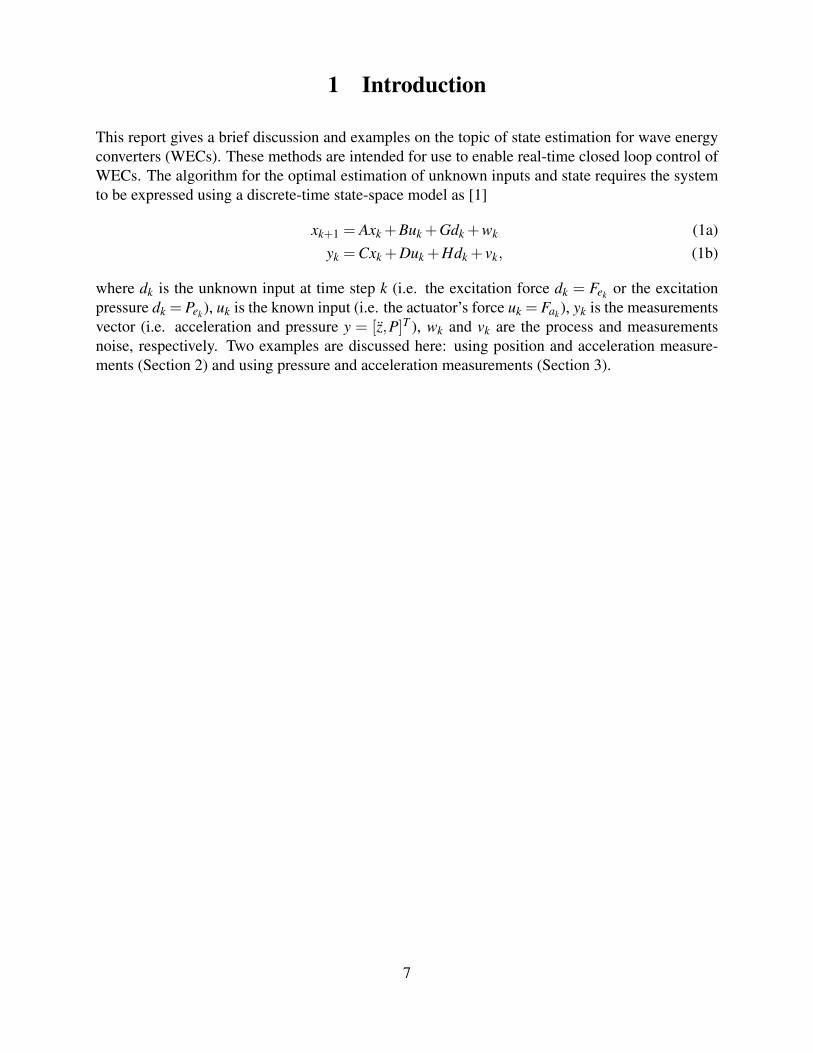
This report gives a brief discussion and examples on the topic of state estimation for wave energyconverters (WECs). These methods are intended for use to enable real-time closed loop control ofWECs. The algorithm for the optimal estimation of unknown inputs and state requires the systemto be expressed using a discrete-time state-space model as [1]
xk+1 = Axk +Buk +Gdk +wk (1a)yk =Cxk +Duk +Hdk + vk, (1b)
where dk is the unknown input at time step k (i.e. the excitation force dk = Fek or the excitationpressure dk = Pek), uk is the known input (i.e. the actuator’s force uk = Fak), yk is the measurementsvector (i.e. acceleration and pressure y = [z,P]T ), wk and vk are the process and measurementsnoise, respectively. Two examples are discussed here: using position and acceleration measure-ments (Section 2) and using pressure and acceleration measurements (Section 3).
7

2 Using position
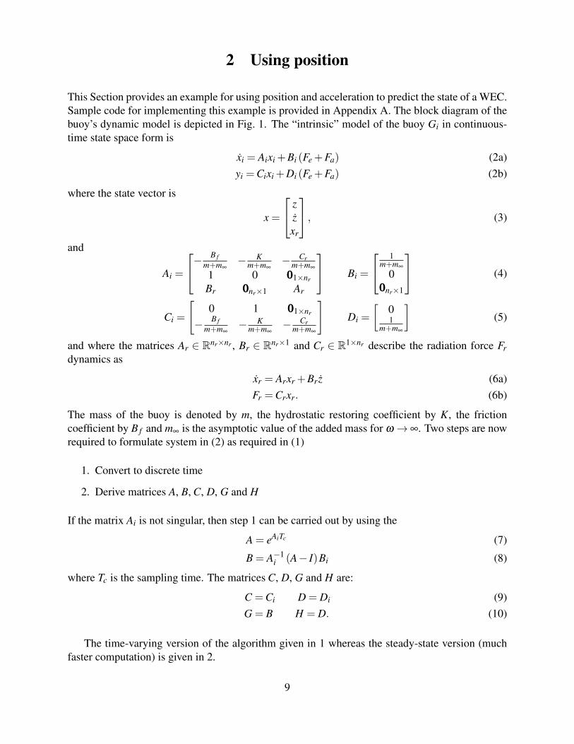
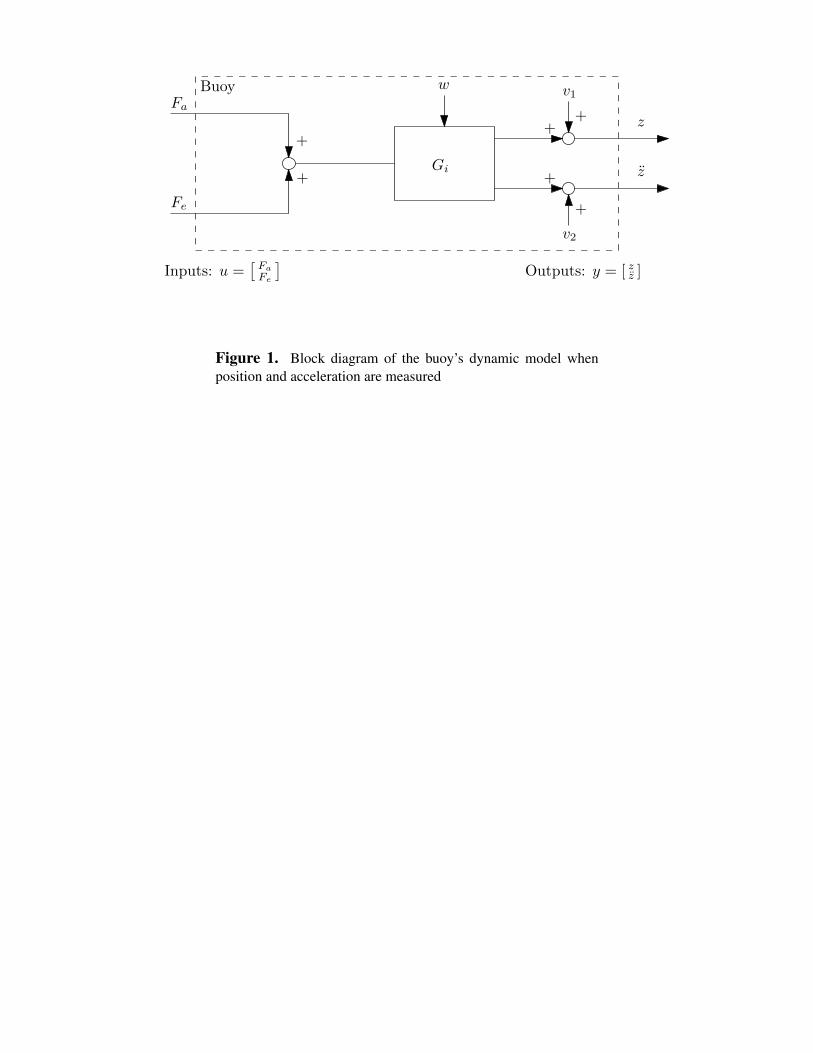
This Section provides an example for using position and acceleration to predict the state of a WEC.Sample code for implementing this example is provided in Appendix A. The block diagram of thebuoy’s dynamic model is depicted in Fig. 1. The “intrinsic” model of the buoy Gi in continuous-time state space form is
xi = Aixi +Bi (Fe +Fa) (2a)yi =Cixi +Di (Fe +Fa) (2b)
where the state vector is
x =
zzxr
, (3)
and
Ai =
− B f
m+m∞− K
m+m∞− Cr
m+m∞
1 0 0001×nr
Br 000nr×1 Ar
Bi =
1m+m∞
0000nr×1
(4)
Ci =
[0 1 0001×nr
− B fm+m∞
− Km+m∞
− Crm+m∞
]Di =
[01
m+m∞
](5)
and where the matrices Ar ∈ Rnr×nr , Br ∈ Rnr×1 and Cr ∈ R1×nr describe the radiation force Frdynamics as
xr = Arxr +Br z (6a)Fr =Crxr. (6b)
The mass of the buoy is denoted by m, the hydrostatic restoring coefficient by K, the frictioncoefficient by B f and m∞ is the asymptotic value of the added mass for ω→∞. Two steps are nowrequired to formulate system in (2) as required in (1)
1. Convert to discrete time
2. Derive matrices A, B, C, D, G and H
If the matrix Ai is not singular, then step 1 can be carried out by using the
A = eAiTc (7)
B = A−1i (A− I)Bi (8)
where Tc is the sampling time. The matrices C, D, G and H are:
C =Ci D = Di (9)G = B H = D. (10)
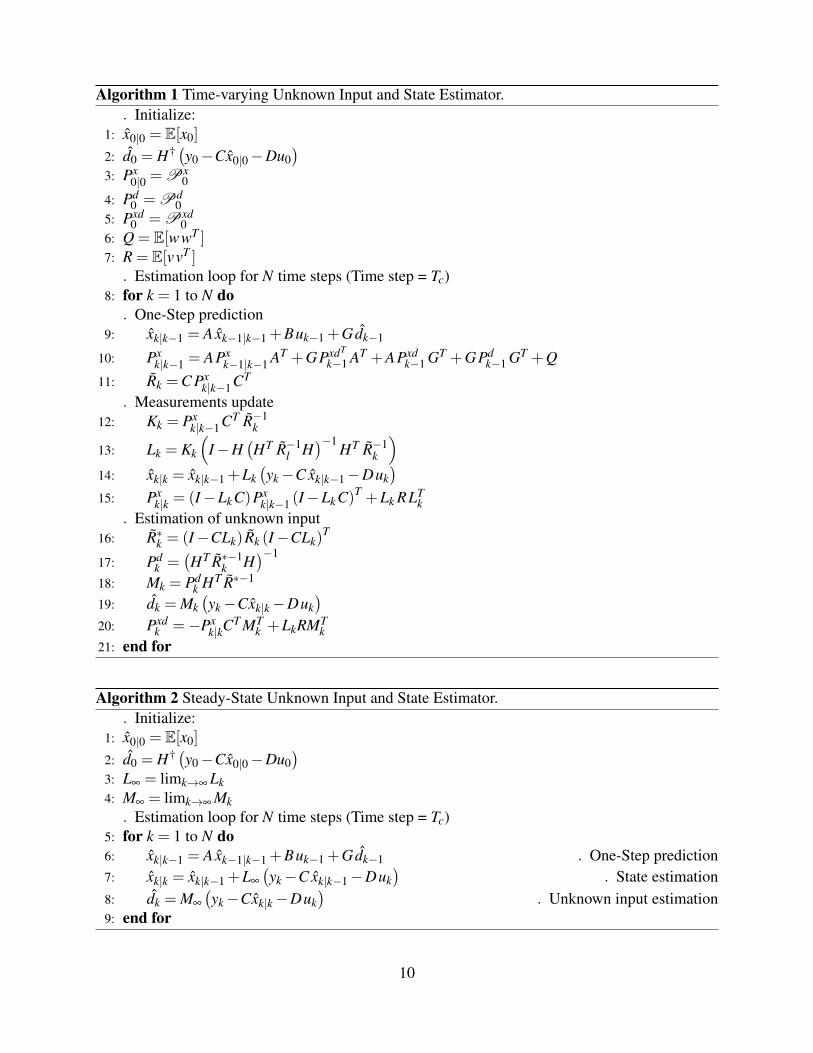
The time-varying version of the algorithm given in 1 whereas the steady-state version (muchfaster computation) is given in 2.
9
Algorithm 1 Time-varying Unknown Input and State Estimator.. Initialize:
1: x0|0 = E[x0]
2: d0 = H† (y0−Cx0|0−Du0)
3: Px0|0 = Px
0
4: Pd0 = Pd
05: Pxd
0 = Pxd0
6: Q = E[wwT ]7: R = E[vvT ]
. Estimation loop for N time steps (Time step = Tc)8: for k = 1 to N do
. One-Step prediction9: xk|k−1 = Axk−1|k−1 +Buk−1 +Gdk−1
10: Pxk|k−1 = APx
k−1|k−1 AT +GPxdT
k−1 AT +APxdk−1 GT +GPd
k−1 GT +Q11: Rk =C Px
k|k−1CT
. Measurements update12: Kk = Px
k|k−1CT R−1k
13: Lk = Kk
(I−H
(HT R−1
l H)−1
HT R−1k
)
14: xk|k = xk|k−1 +Lk(yk−C xk|k−1−Duk
)
15: Pxk|k = (I−Lk C)Px
k|k−1 (I−Lk C)T +Lk RLTk
. Estimation of unknown input16: R∗k = (I−CLk) Rk (I−CLk)
T
17: Pdk =
(HT R∗−1
k H)−1
18: Mk = Pdk HT R∗−1
19: dk = Mk(yk−Cxk|k−Duk
)
20: Pxdk =−Px
k|kCT MT
k +LkRMTk
21: end for
Algorithm 2 Steady-State Unknown Input and State Estimator.. Initialize:
1: x0|0 = E[x0]
2: d0 = H† (y0−Cx0|0−Du0)
3: L∞ = limk→∞ Lk4: M∞ = limk→∞ Mk
. Estimation loop for N time steps (Time step = Tc)5: for k = 1 to N do6: xk|k−1 = Axk−1|k−1 +Buk−1 +Gdk−1 . One-Step prediction7: xk|k = xk|k−1 +L∞
(yk−C xk|k−1−Duk
). State estimation
8: dk = M∞
(yk−Cxk|k−Duk
). Unknown input estimation
9: end for
10
Fa
z+
+
Outputs: y = [ zz ]Inputs: u =[Fa
Fe
]
Buoy
+
+
v2
v1
+
+
Fe
zGi
w
Figure 1. Block diagram of the buoy’s dynamic model whenposition and acceleration are measured
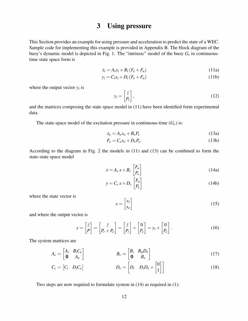
3 Using pressure
This Section provides an example for using pressure and acceleration to predict the state of a WEC.Sample code for implementing this example is provided in Appendix B. The block diagram of thebuoy’s dynamic model is depicted in Fig. 1. The “intrinsic” model of the buoy Gi in continuous-time state space form is
xi = Aixi +Bi (Fe +Fa) (11a)yi =Cixi +Di (Fe +Fa) (11b)
where the output vector yi is
yi =
[zPr
], (12)
and the matrices composing the state space model in (11) have been identified form experimentaldata.
The state-space model of the excitation pressure in continuous-time (Ge) is:
xe = Aexe +BePe (13a)Fe =Cexe +DePe. (13b)
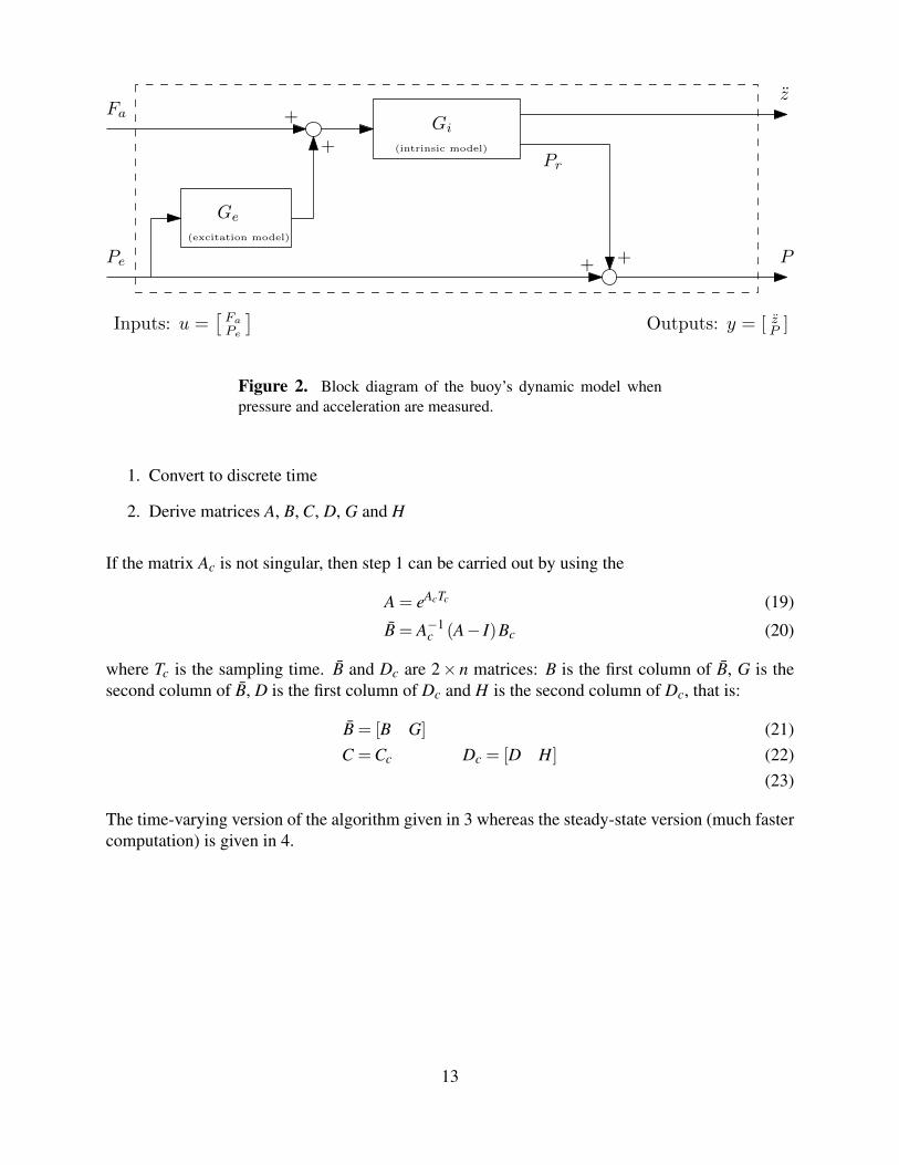
According to the diagram in Fig. 2 the models in (11) and (13) can be combined to form thestate-state space model
x = Ac x+Bc
[FaPe
](14a)
y =Cc x+Dc
[FaPe
](14b)
where the state vector is
x =[
xixe
](15)
and where the output vector is
y =[
zP
]=
[z
Pr +Pe
]=
[zPr
]+
[0Pe
]= yi +
[0Pe
]. (16)
The system matrices are
Ac =
[Ai BiCe000 Ae
]Bc =
[Bi BuDe000 Be
](17)
Cc =[Ci DiCe
]Dc =
[Di DiDe +
[01
]](18)
Two steps are now required to formulate system in (14) as required in (1):
12
Gi
Ge
Fa
Pe P
z+
+
++
(intrinsic model)
(excitation model)
Outputs: y = [ zP ]Inputs: u =[Fa
Pe
]
Pr
Figure 2. Block diagram of the buoy’s dynamic model whenpressure and acceleration are measured.
1. Convert to discrete time
2. Derive matrices A, B, C, D, G and H
If the matrix Ac is not singular, then step 1 can be carried out by using the
A = eAcTc (19)
B = A−1c (A− I)Bc (20)
where Tc is the sampling time. B and Dc are 2× n matrices: B is the first column of B, G is thesecond column of B, D is the first column of Dc and H is the second column of Dc, that is:
B = [B G] (21)C =Cc Dc = [D H] (22)
(23)
The time-varying version of the algorithm given in 3 whereas the steady-state version (much fastercomputation) is given in 4.
13

Algorithm 3 Time-varying Unknown Input and State Estimator.. Initialize:
1: x0|0 = E[x0]
2: d0 = H† (y0−Cx0|0−Du0)
3: Px0|0 = Px
0
4: Pd0 = Pd
05: Pxd
0 = Pxd0
6: Q = E[wwT ]7: R = E[vvT ]
. Estimation loop for N time steps (Time step = Tc)8: for k = 1 to N do
. One-Step prediction9: xk|k−1 = Axk−1|k−1 +Buk−1 +Gdk−1
10: Pxk|k−1 = APx
k−1|k−1 AT +GPxdT
k−1 AT +APxdk−1 GT +GPd
k−1 GT +Q11: Rk =C Px
k|k−1CT
. Measurements update12: Kk = Px
k|k−1CT R−1k
13: Lk = Kk
(I−H
(HT R−1
l H)−1
HT R−1k
)
14: xk|k = xk|k−1 +Lk(yk−C xk|k−1−Duk
)
15: Pxk|k = (I−Lk C)Px
k|k−1 (I−Lk C)T +Lk RLTk
. Estimation of unknown input16: R∗k = (I−CLk) Rk (I−CLk)
T
17: Pdk =
(HT R∗−1
k H)−1
18: Mk = Pdk HT R∗−1
19: dk = Mk(yk−Cxk|k−Duk
)
20: Pxdk =−Px
k|kCT MT
k +LkRMTk
21: end for
Algorithm 4 Steady-State Unknown Input and State Estimator.. Initialize:
1: x0|0 = E[x0]
2: d0 = H† (y0−Cx0|0−Du0)
3: L∞ = limk→∞ Lk4: M∞ = limk→∞ Mk
. Estimation loop for N time steps (Time step = Tc)5: for k = 1 to N do6: xk|k−1 = Axk−1|k−1 +Buk−1 +Gdk−1 . One-Step prediction7: xk|k = xk|k−1 +L∞
(yk−C xk|k−1−Duk
). State estimation
8: dk = M∞
(yk−Cxk|k−Duk
). Unknown input estimation
9: end for
14
References
[1] Sze Zheng Yong, Minghui Zhu, and Emilio Frazzoli. A unified filter for simultaneous inputand state estimation of linear discrete-time stochastic systems. Automatica, 63:321 – 329,2016.
15

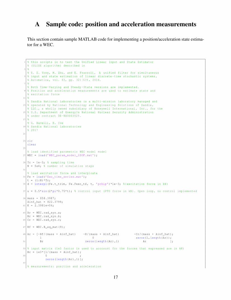
A Sample code: position and acceleration measurements
This section contain sample MATLAB code for implementing a position/acceleration state estima-tor for a WEC.
1 % this scripts is to test the Unified Linear Input and State Estimator% (ULISE algorithm) described in
3 %% S. Z. Yong , M. Zhu, and E. Frazzoli , A unified filter for simultaneous
5 % input and state estimation of linear discrete -time stochastic systems ,% Automatica , vol. 63, pp. 321 329 , 2016.
7 %% Both Time -Varying and Steady -State versions are implemented.
9 % Position and acceleration measurements are used to estimate state and% excitation force
11 %% Sandia National Laboratories is a multi -mission laboratory managed and
13 % operated by National Technology and Engineering Solutions of Sandia ,% LLC., a wholly owned subsidiary of Honeywell International , Inc., for the
15 % U.S. Department of Energy?s National Nuclear Security Administration% under contract DE-NA0003525.
17 %% G. Bacelli , R. Coe
19 % Sandia National Laboratories% 2017
21
23 clcclear
25
% load identified parametric WEC model model27 WEC = load(’WEC_param_model_1DOF.mat’);
29 Tc = 1e-3; % sampling timeN = 5e4; % number of simulation steps
31
% load excitation force and interploate33 Fe = load(’Exc_time_series.mat’);
t = (1:N)*Tc;35 d = interp1(Fe.t_trim , Fe.Fexc_td , t, ’pchip’)*1e-3; %(excitation force in kN)
37 u = 0.5*sin(2*pi*0.75*t); % control input (PTO force in kN). Open loop , no control implemented
39 mass = 858.3987;Ainf_hat = 822.3799;
41 K = 2.3981e+04;
43 Ar = WEC.rad_sys.a;Br = WEC.rad_sys.b;
45 Cr = WEC.rad_sys.c;
47 Bf = WEC.B_eq_mat(9);
49 Ac = [-Bf/(mass + Ainf_hat) -K/(mass + Ainf_hat) -Cr/(mass + Ainf_hat);1 0 zeros(1,length(Ar));
51 Br zeros(length(Ar),1) Ar ];
53 % input matrix (1e3 factor is used to acccount for the forces that expressed are in kN)Bc = 1e3*[1/(mass + Ainf_hat);
55 0 ;zeros(length(Ar),1)];
57
% measurements: position and acceleration
17
59 C = [0 1 zeros(1,length(Ar));Ac(1,:) ];
61
D = [0; Bc(1)];63
n = size(C,2);65 p = size(C,1);
67 % convert continuous time model to discrete timeA = expm(Ac*Tc);
69 B = Ac\(A - eye(n))*Bc;
71 G = B;H = D;
73
% process noise75 w = .00001*(rand(N,4) -0.5);
% measurements noise77 v = (rand(N,p) -0.5) * diag([.0001 ,0.05]);
79 Q = cov(w);R = cov(v);
81
%% Time varying filter83
% initialize variables85 P_x_k_k = 0.001*eye(n);
P_xd_k = 0.001*ones(n,1);87 P_d_k = 0.001;
89 x = zeros(n,1);x_k_k = x;
91 d_k = 0;
93 In = eye(n);Ip = eye(p);
95
% preallocation97 d_k_vec = zeros(N,1);
x_k_vec = zeros(n,N);99 x_vec = zeros(n,N);
y_vec = zeros(p,N);101
103 tic
105 for ii = 1:N
107 x = A*x + B*u(ii) + G*d(ii) + w(ii ,:) ’;y = C*x + D*u(ii) + H*d(ii) + v(ii ,:) ’;
109
x_vec(:,ii) = x;111 y_vec(:,ii) = y;
113 x_k_k1 = A*x_k_k + B*u(ii) + G*d_k;P_x_k_k1 = A*P_x_k_k*A’ + G*P_xd_k ’*A’ + A*P_xd_k*G’ + G*P_d_k*G’ + Q;
115 R_t_k = C*P_x_k_k1*C’ + R;Kk = P_x_k_k1*C’/R_t_k;
117 Lk = Kk*(Ip -((H/((H’/R_t_k)*H))*H’/R_t_k ));x_k_k = x_k_k1 + Lk*(y - C*x_k_k1 - D*u(ii) );
119 P_x_k_k = (In-Lk*C)*P_x_k_k1*(In-Lk*C)’ + Lk*R*Lk’;R_ts_k = (Ip-C*Lk)*R_t_k*(Ip-C*Lk)’;
121 P_d_k = inv((H’/R_ts_k)*H);Mk = ((H’/R_ts_k)*H)\(H’/R_ts_k);
123 d_k = Mk*(y - C*x_k_k - D*u(ii));P_xd_k = -P_x_k_k*C’*Mk’ + Lk*R*Mk’;
125
d_k_vec(ii) = d_k;
18
127 x_k_vec(:,ii) = x_k_k;
129 end
131 t_tv = toc;disp(’done TV’)
133
%% steady state filter135
L_inf = Lk;137 M_inf = Mk;
139 % preallocationd_k_vec_inf = zeros(N,1);
141 x_vec_inf = zeros(n,N);y_vec_inf = zeros(p,N);
143 x_vec_est_inf = x_vec_inf;
145 % initializationx = zeros(n,1);
147 x_k_k_inf = zeros(n,1);d_k1_inf = 0;
149
tic151 for ii = 1:N
153 x = A*x + B*u(ii) + G*d(ii) + w(ii ,:) ’;y = C*x + D*u(ii) + H*d(ii) + v(ii ,:) ’;
155
x_vec_inf(:,ii) = x;157 y_vec_inf(:,ii) = y;
159 x_k_k1_inf = A*x_k_k_inf + B*u(ii) + G*d_k1_inf;x_k_k_inf = x_k_k1_inf + L_inf*(y - C*x_k_k1_inf - D*u(ii) );
161 d_k1_inf = M_inf*(y - C*x_k_k_inf - D*u(ii));
163 d_k_vec_inf(ii) = d_k1_inf;x_vec_est_inf(:,ii) = x_k_k_inf;
165 end
167 t_ss = toc;disp(’done SS’)
169
171 %% plotting
173 disp([’Time to compute Time -Varying filter: ’ num2str(t_tv) ’s’])disp([’Time to compute Steady -State filter: ’ num2str(t_ss) ’s’])
175
figure(1)177 plot(t, d_k_vec ’, t, d)
xlabel(’time (s)’)179 ylabel(’(kN)’)
grid on181 title(’Time -Varying filter’)
legend({’${\hat{F}e}_{\infty}$’, ’$Fe$’}, ’Interpreter’, ’latex’)183
figure(2)185 plot(t, d_k_vec_inf , t, d)
xlabel(’time (s)’)187 ylabel(’(kN)’)
grid on189 title(’Steady -State filter’)
legend({’$\hat{F}e$’, ’$Fe$’}, ’Interpreter’, ’latex’)191
figure(3)193 plot(t, d_k_vec - d_k_vec_inf)
grid on
19
195 xlabel(’Time (s)’)title(’Difference between Time -Varying and Steady -State filters’)
197 legend(’e_d’)
199 figure(4)subplot 211
201 plot(t, y_vec(1,:) ’)xlabel(’Time (s)’)
203 ylabel(’(m)’)title(’Measured (noisy) Outputs’)
205 legend({’$z$’}, ’Interpreter’, ’latex’)grid on
207 subplot 212plot(t, y_vec(2,:) ’)
209 xlabel(’Time (s)’)ylabel(’(m/sˆ2)’)
211 legend({’$\ddot{z}$’}, ’Interpreter’, ’latex’)grid on
213
215 figure(5)subplot 211
217 plot(t, x_vec(1,:)’, t, x_k_vec(1,:)’, t, x_vec_est_inf(1,:) ’)grid on
219 xlabel(’time (s)’)ylabel(’(m/s)’)
221 legend({’$v$’, ’$\hat{v}$’, ’$\hat{v}_{\infty}$’}, ’Interpreter’, ’latex’)title(’Estimated states’)
223 grid on
225 subplot 212plot(t, x_vec(2,:)’, t, x_k_vec(2,:)’, t, x_vec_est_inf(2,:) ’)
227 grid onxlabel(’time (s)’)
229 ylabel(’(m)’)legend({’$z$’, ’$\hat{z}$’, ’$\hat{z}_{\infty}$’}, ’Interpreter’, ’latex’)
231 grid on
State and unknown input estimator position acceleration.m
20
B Sample code: pressure and acceleration measurements
This section contain sample MATLAB code for implementing a pressure/acceleration state esti-mator for a WEC.
1 % this scripts is to test the Unified Linear Input and State Estimator% (ULISE algorithm) described in
3 %% S. Z. Yong , M. Zhu, and E. Frazzoli , A unified filter for simultaneous
5 % input and state estimation of linear discrete -time stochastic systems ,% Automatica , vol. 63, pp. 321 329 , 2016.
7 %% Both Time -Varying and Steady -State versions are implemented. Pressure and
9 % acceleration measurements are used to estimate state and excitation force%
11 % Sandia National Laboratories is a multi -mission laboratory managed and% operated by National Technology and Engineering Solutions of Sandia ,
13 % LLC., a wholly owned subsidiary of Honeywell International , Inc., for the% U.S. Department of Energy?s National Nuclear Security Administration
15 % under contract DE-NA0003525.%
17 % G. Bacelli , R. Coe% Sandia National Laboratories
19 % 2017
21
clc23 clear
25 % load identified parametric WEC model modelWEC = load(’WEC_param_model_1DOF.mat’); % radiatiojn impedance model
27 Gr = struct2array(load(’Gr_model.mat’)); % radiation pressure modelGe = struct2array(load(’Ge_model.mat’)); % excitation pressure model
29
Tc = 1e-3;31 N = 5e4;
33 % load excitation forceFe = load(’Exc_time_series.mat’); %(excitation force in kN)
35 t = (1:N)*Tc;d = interp1(Fe.t_trim , Fe.Fexc_td , t, ’pchip’)*1e-3; % control input (PTO force in kN). Open loop
, no control implemented37
u = .5*sin(2*pi*0.75*t);39
mass = 858.3987;41 Ainf_hat = 822.3799;
K = 2.3981e+04;43
Ar = WEC.rad_sys.a;45 Br = WEC.rad_sys.b;
Cr = WEC.rad_sys.c;47
Bf = WEC.B_eq_mat(9);49
Am = [-Bf/(mass + Ainf_hat) -K/(mass + Ainf_hat) -Cr/(mass + Ainf_hat);51 1 0 zeros(1,length(Ar));
Br zeros(length(Ar),1) Ar];53
% input matrix (1e3 factor is used to acccount for the forces that expressed are in kN)55 Bm = 1e3*[1/(mass + Ainf_hat);
0 ;57 zeros(length(Ar),1) ];
21
59 Cm = Am(1,:);
61 Dm = Bm(1);
63 Ai = blkdiag(Am, Gr.A);Bi = [Bm; Gr.B];
65 Ci = blkdiag(Cm, Gr.C);Di = [Dm; Gr.D];
67
ni = size(Ai ,1);69 ne = size(Ge.A,1);
Ac = [Ai, Bi*Ge.C;71 zeros(ne, ni) Ge.A];
73 Bc = [Bi, Bi*Ge.D; zeros(ne ,1), Ge.B];
75 C = [Ci, Di*Ge.C];D = [Di, Di*Ge.D + [0;1] ];
77
sys_c = ss(Ac, Bc, C, D);79 sys_d = c2d(sys_c , Tc);
81 Ge_d = c2d(Ge,Tc);
83 Ce = Ge_d.C;De = Ge_d.D;
85
n = size(C,2);87 p = size(C,1);
89 % convert continuous time model to discrete timeA = expm(Ac*Tc);
91 B = Ac\(A - eye(n))*Bc;
93 G = B(:,1);B = B(:,1);
95
H = D(:,2);97 D = D(:,1);
99 % process noisew = .00001*(rand(N,ni+ne) -0.5);
101 % measurements noisev = (rand(N,p) -0.5) * diag([.05, 0.05]);
103
Q = cov(w);105 R = cov(v);
107 %% Time Varying filter
109 % initialize variablesP_x_k_k = 0.001*eye(n);
111 P_xd_k = 0.001*ones(n,1);P_d_k = 0.001;
113
x = zeros(n,1);115 x_k_k = x;
d_k = 0;117
In = eye(n);119 Ip = eye(p);
121 % preallocationx_vec = zeros(n,N);
123 y_vec = zeros(p,N);d_k_vec = zeros(N,1);
125 x_k_vec = zeros(n,N);
22
Fe_est = zeros(N,1);127 Fe = Fe_est;
129 tic
131 for ii = 1:N
133 x = A*x + B*u(ii) + G*d(ii) + w(ii ,:) ’;y = C*x + D*u(ii) + H*d(ii) + v(ii ,:) ’;
135
Fe(ii) = Ce*x(ni+1:end) + De*d(ii);137
x_vec(:,ii) = x;139 y_vec(:,ii) = y;
141 x_k_k1 = A*x_k_k + B*u(ii) + G*d_k;P_x_k_k1 = A*P_x_k_k*A’ + G*P_xd_k ’*A’ + A*P_xd_k*G’ + G*P_d_k*G’ + Q;
143 R_t_k = C*P_x_k_k1*C’ + R;Kk = P_x_k_k1*C’/R_t_k;
145 Lk = Kk*(Ip -((H/((H’/R_t_k)*H))*H’/R_t_k ));x_k_k = x_k_k1 + Lk*(y - C*x_k_k1 - D*u(ii) );
147 P_x_k_k = (In-Lk*C)*P_x_k_k1*(In-Lk*C)’ + Lk*R*Lk’;R_ts_k = (Ip-C*Lk)*R_t_k*(Ip-C*Lk)’;
149 P_d_k = inv((H’/R_ts_k)*H);Mk = ((H’/R_ts_k)*H)\(H’/R_ts_k);
151 d_k = Mk*(y - C*x_k_k - D*u(ii));P_xd_k = -P_x_k_k*C’*Mk’ + Lk*R*Mk’;
153
d_k_vec(ii) = d_k;155 x_k_vec(:,ii) = x_k_k;
Fe_est(ii) = Ce*x_k_k(ni+1:end) + De*d_k;157
end159
t_tv = toc;161 disp(’done TV’)
163 %% Steady State filter
165 L_inf = Lk;M_inf = Mk;
167
% preallocation169 d_k_vec_inf = zeros(N,1);
x_vec_inf = zeros(n,N);171 y_vec_inf = zeros(p,N);
x_vec_est_inf = x_vec_inf;173 Fe_est_inf = zeros(N,1);
175 % initializationx = zeros(n,1);
177 x_k_k_inf = zeros(n,1);d_k1_inf = 0;
179
tic181 for ii = 1:N
183 x = A*x + B*u(ii) + G*d(ii) + w(ii ,:) ’;y = C*x + D*u(ii) + H*d(ii) + v(ii ,:) ’;
185
x_vec_inf(:,ii) = x;187 y_vec_inf(:,ii) = y;
189 x_k_k1_inf = A*x_k_k_inf + B*u(ii) + G*d_k1_inf;x_k_k_inf = x_k_k1_inf + L_inf*(y - C*x_k_k1_inf - D*u(ii) );
191 d_k1_inf = M_inf*(y - C*x_k_k_inf - D*u(ii));
193 d_k_vec_inf(ii) = d_k1_inf;
23
x_vec_est_inf(:,ii) = x_k_k_inf;195 Fe_est_inf(ii) = Ce*x_k_k_inf(ni+1:end) + De*d_k1_inf;
end197
t_ss = toc;199 disp(’done SS’)
201 %% plotting
203 disp([’Time to compute Time -Varying filter: ’ num2str(t_tv) ’s’])disp([’Time to compute Steady -State filter: ’ num2str(t_ss) ’s’])
205
207 figure(1)subplot 211
209 plot(t, d_k_vec ’, t, d)xlabel(’time (s)’)
211 ylabel(’(kPa)’)grid on
213 legend({’$\hat{P}e$’, ’$Pe$’ }, ’Interpreter’, ’latex’)title(’Time -Varying filter: Unknown input (Excitation pressure Pe)’)
215
subplot 212217 plot(t, Fe_est , t, Fe)
grid on219 ylabel(’(kN)’)
xlabel(’time (s)’)221 title(’Excitation force’)
legend({’$\hat{F}e$’, ’$Fe$’}, ’Interpreter’, ’latex’)223
figure(2)225 subplot 211
plot(t, d_k_vec_inf ’, t, d)227 xlabel(’time (s)’)
ylabel(’(kPa)’)229 grid on
legend({’$\hat{P}e$’, ’$Pe$’ }, ’Interpreter’, ’latex’)231 title(’Steady -State filter: Unknown input (Excitation pressure Pe)’)
233 subplot 212plot(t, Fe_est_inf , t, Fe)
235 grid onylabel(’(kN)’)
237 xlabel(’time (s)’)title(’Excitation force’)
239 legend({’$\hat{F}e$’, ’$Fe$’}, ’Interpreter’, ’latex’)
241 figure(3)plot(t, d_k_vec - d_k_vec_inf)
243 grid onxlabel(’Time (s)’)
245 title(’Difference between Time -Varying and Steady -State filters’)legend(’e_d’)
247
figure(4)249 subplot 211
plot(t, y_vec(1,:) ’)251 xlabel(’Time (s)’)
ylabel(’(m/sˆ2)’)253 title(’Measured (noisy) Outputs’)
legend({’$\ddot{z}$’}, ’Interpreter’, ’latex’)255 grid on
subplot 212257 plot(t, y_vec(2,:) ’)
xlabel(’Time (s)’)259 ylabel(’(kPa)’, ’Interpreter’, ’latex’)
grid on261 legend({’$P$’}, ’Interpreter’, ’latex’)
24
263 figure(5)subplot 211
265 plot(t, x_vec(1,:)’, t, x_k_vec(1,:)’, t, x_vec_est_inf(1,:) ’)grid on
267 xlabel(’time (s)’)ylabel(’(m/s)’)
269 legend({’$v$’, ’$\hat{v}$’, ’$\hat{v}_{\infty}$’}, ’Interpreter’, ’latex’)title(’Estimated states’)
271 grid on
273 subplot 212plot(t, x_vec(2,:)’, t, x_k_vec(2,:)’, t, x_vec_est_inf(2,:) ’)
275 grid onxlabel(’time (s)’)
277 ylabel(’(m)’)legend({’$z$’, ’$\hat{z}$’, ’$\hat{z}_{\infty}$’}, ’Interpreter’, ’latex’)
279 grid on
State and unknown input estimator pressure acceleration.m
25

DISTRIBUTION:
1 MS 0899 Technical Library, 9536 (electronic copy)
26

v1.40
27

28