Further Analyses of the Exercise and Cost Impacts of Market PowerIn California’s Wholesale Energy Market

March 2001

Prepared by

Eric Hildebrandt, Ph.D.

Department of Market Analysis

California Independent System Operator Corporation

2

Executive Summary

This report provides the results of additional analyses undertaken by the CaliforniaIndependent System Operator Corporation’s Department of Market Analysis (“DMA”) ofthe exercise and impact of market power in California’s wholesale energy markets.

First, additional analysis of the impact of market power on overall wholesale energyprices is presented based on the price cost markup.1 In this analysis, the potentialimpacts of NOx emissions costs and hours of potential resource scarcity are explicitlyincorporated into the analysis. Results show that after incorporating potential NOxcosts and hours of resource scarcity into the analysis, over 30% of wholesale energycosts over the last year can be attributed to market power, or a level that clearlyexceeds the range that may be consistent with a workably competitive market. Theresults clearly show that market power is not limited to hours when a deficiency inoperating reserves requires the ISO to declare the existence of a System Emergency.The resulting prices represent potential additional net costs to consumers of about $6.8billion. About 80% of these additional costs are attributable to non-emergency hourswhen the ISO has not declared Stage 3 conditions.

Second, wholesale prices are examined in relation to the cost of investment in newsupply. Regulators and others have expressed concern that prices be sufficient tomake investments in new supply profitable, so that the entry of additional supply isencouraged. Results of this analysis indicate that prices over the last 12 months havesignificantly exceeded the cost of new supply options. On an annualized basis,wholesale energy prices since January 2000 are exceeding the cost necessary for newinvestment by about 400%, and would allow recovery of an investment in new supply ina period of less than two years. Thus, this analysis indicates that market powermitigation plans can be adopted and designed to reduce significantly wholesale pricesobserved over the last year, while still providing sufficient opportunity for recovery ofcosts in new investment.

1. Background

Previous DMA analyses have shown that the high prices observed since May 2000have been due to the exercise of market power, in combination with several otherunderlying drivers that would be expected to increase costs even under perfectly

1 Previous analysis of market power based on price-cost markup was included in Comments of the ISO

on November 1, 2000 Order ("November 1 Order"), Attachment A, November 22, 2000. Results of thisanalysis are consistent with other filings at FERC based on the price cost markup, including “DiagnosingMarket Power in California’s Restructured Electricity Markets”, (Borenstein, Bushnell, and Wolak),August 2000; Updated results through June 2000 presented in An Analysis of the June 2000 PriceSpikes in the California ISO’s Energy and Ancillary Service Markets, MSC Report, September 6, 2000;and A Quantitative Analysis of Pricing Behavior in California’s Wholesale Electricity Market DuringSummer 2000, P. Joskow and E. Kahn, November 21, 2000.

3

competitive conditions. DMA has developed and presented analyses specificallydesigned to differentiate between market costs incurred as a result of the exercise ofmarket power, rather than other underlying drivers of cost, including absolute scarcityfor capacity during some hours. For instance, in an August 10, 2000 report provided toFERC in the context of the Commission’s Investigation of Western Bulk Power Marketsthe DMA noted that:

…there are many hours of extremely high prices when supply and demand arerelatively tight, but there is no apparent shortage of supply. During these hourshigh prices are most likely the result of market power. The presence of marketpower can be verified by a high bid price over variable cost by many suppliers inthe ISO’s markets. The highest variable cost of in-state generators is below$100/MWh, while many suppliers routinely bid a significant part of their capacity at$750 (the price cap level). These bids had to be selected to meet the demandduring high load periods. (p.51) 3

The DMA’s August 10 report further explained that:

The observed market power was the combined effect of the bidding activity of in-state and out-of-state generation resources. The available data and tools do notallow detailed analysis of the market power of out-of-state generation owners. TheISO, however, is not aware of any acute regional shortages in most of the highprice hours. The high prices bid by out-of-state suppliers as well as the highprices quoted to ISO’s out-of-market calls are indications of the market power ofout-of-state suppliers. (p. 5)

Subsequently, in a report filed with FERC on October 20, 2000, DMA staff presentedresults of a more systematic, quantitative analyses of market power and any potentialscarcity of supply within the CAISO system over the CAISO’s first two and one halfyears of operation. Results of this analysis showed significant degree of market powerduring the months of May to September 2000, and noted that:

While a significant portion of the increase in wholesale costs above thiscompetitive baseline have been incurred during hours of potential absoluteresource scarcity, the bulk of these additional costs are attributable a lack ofcompetition, rather than scarcity. In addition, prices continued to significantlyexceed competitive levels even after the ISO’s real time price cap was lowered to$250 in August. (p.5)

A DMA report submitted with the ISO’s comments on the Commission’s November 1Order presented the results of quantitative analysis by DMA staff of the impact ofmarket power and other factors on market costs. As explained in this report by theDMA:

[S]ince late May of this year [2000], the combination of very tight supply anddemand conditions — in conjunction with very limited ability of consumers to

4

reduce consumption in response to high prices — has created the opportunity forthe persistent exercise of market power in California’s wholesale energy markets.The exercise of this market power has inflated wholesale energy costs significantlyabove levels that would have resulted under competitive market conditions, evenafter taking into account fundamental market factors driving up costs and hours ofpotential scarcity of supply. While some degree of market power may be tolerablefrom the perspective of defining a workably competitive market, the exercise ofmarket power since late May of this year has clearly exceeded the level that maybe considered consistent with a workably competitive market. Since additions ofnew supply are likely to merely keep pace with or even fall short of demand growthover the next two years, the exercise of significant market power can be expectedto continue – if not worsen – over the next two years absent action to moreeffectively mitigate system-wide market power. 2

The ISO’s comments further emphasized that that “the ISO believes market outcomesin summer 2000 clearly demonstrate that market power was exercised, and thatunrestricted market-based rate authority will continue to results in prices which areunjust and unreasonable.” (p.15)

This report provides further analyses of the exercise and impact of market power inCalifornia’s wholesale energy markets. The additional analysis addresses points orconcerns that have been raised before the Federal Energy Regulatory Commission(FERC) through written public comments, the FERC staff report and, most recently, thetechnical conference on market power mitigation held January 23, 2000.

• Section 2 presents additional analysis of the impact of market power on overallsystem prices and is presented based on the price cost markup. In this analysis, thepotential impacts of NOx emissions constraints is explicitly incorporated into theanalysis.

• Section 3 examines wholesale prices in relation to the cost of investment in newsupply. The results of this analysis indicate that there is ample room to reducesignificantly wholesale prices observed over the last year, while still providingsufficient opportunity for recovery of costs in new investment.

2 California Independent System Operator, Comments on FERC’s November 1 Order on ProposedRemedies for California’s Wholesale Markets, Attachment A: Analysis of Market Power in California’sWholesale Energy Markets, filed November 22, 2000.

5

2. Comparison of Market Costs with Competitive Baseline

Most economists agree that – at least in the short run --- the competitive price is short-run marginal costs, and that the competitive benchmark for assessing market power isthe short-run marginal costs of the highest cost unit needed to meet demand. Theoverall impact of the exercise of market power on California’s energy markets has beenassessed in several studies, by DMA and others, using variations of a similar price costmarkup methodology, which compares energy prices to the variable cost of the marginalunit needed to meet demand.3 Results of these studies consistently show thatwholesale prices in the PX Day Ahead and ISO real time markets have beensignificantly in excess of competitive levels over the last year, even after accounting forair emission costs4 and scarcity.5

This section provides updated and expanded results of previous analyses by DMA.This analysis is based on the same basic approach described in previous reportssubmitted to FERC.6 Figure 2-1 illustrates and provides further descriptions of themethod used to estimate the marginal costs of the highest cost unit needed to meetdemand in the ISO system during each hour. This price represents the market clearingprice that would have prevailed under workably competitive conditions. Additionalanalysis and results presented in this report specifically address the degree to which theextremely high wholesale energy prices can be attributed to environmental emissioncosts and resource scarcity, rather than market power. In addition, severalmodifications have been added to account for the dramatic changes in marketconditions, design and structure starting in December 2000. Refinements to this

3 Borenstein, Severin; Bushnell, James; and Wolak, Frank, “Diagnosing Market Power in California’sRestructured Electricity Markets”, August 2000; Updated results through June 2000 presented in AnAnalysis of the June 2000 Price Spikes in the California ISO’s Energy and Ancillary Service Markets,MSC Report, September 6, 2000.

A Quantitative Analysis of Pricing Behavior in California’s Wholesale Electricity Market During Summer2000, P. Joskow and E. Kahn, November 21, 2000, submitted as attachment to Southern CaliforniaEdison’s Comments on FERC’s November 1 Order on Proposed Remedies for California’s WholesaleMarkets, November 22, 2000.

California Independent System Operator, Comments on FERC’s November 1 Order on ProposedRemedies for California’s Wholesale Markets, Attachment A: Analysis of Market Power in California’sWholesale Energy Markets, filed November 22, 2000.

4 The issue of emissions has been previously addressed in analysis by Joskow and Kahn (2000)submitted as part of these proceedings.

5 The issue of potential scarcity rents was addressed in the ISO’s Report on California Energy MarketIssues and Performance: May-June, 2000, Prepared by the Department of Market Analysis, August 10,2000, and ISO Comments on FERC's November 1 Order, Attachment A: Analysis of Market Power inCalifornia’s Wholesale Energy Markets, filed November 22, 2000.

6 ISO Comments on FERC’s November 1 Order, Attachment A: Analysis of Market Power in California’sWholesale Energy Markets, filed November 22, 2000. Additional background on the method used toassess resource scarcity was provided in the ISO’s Report on California Energy Market Issues andPerformance: May-June, 2000, Prepared by the Department of Market Analysis, August 10, 2000,submitted to FERC as part of its investigation of Western bulk power markets.

6

previous methodology are described in more detail in Appendix A.

Figure 2-1. Price-Cost Markup Methodology

PS Non-Utility Thermal + Other Real Time

MCP Competitive

DEnergy DTotal

QResidual Supply

UDC Generation, QFs, RenewablesMinimum RMR Requirements,and Small Residual Suppliers

The competitive baseline price used in this analysis represents the estimatedvariable operating cost of the highest cost thermal generation unit needed to meetsystem demand each hour.

To estimate this competitive baseline price, the operating costs of major non-utilityowned thermal units within the CAISO system are first estimated based on unit heatrates, spot market gas prices, estimated O&M costs, including NOx emissions. Theavailability of these units each operating day is determined based on outage datareported to the ISO, and whether a unit is in operation and/or bid into the ISOmarkets. Through October 2000, the “supply curve” used in this analysis includesreal time energy bids from imports submitted as Replacement Reserve andSupplemental Energy bids in this supply curve.

The net system demand that must be met by these resources is then calculated foreach hour by first increasing total system loads to account for additional capacityneeded for on-line reserves (about 7% for upward regulation and spinning reserve),as shown in the figure above. The portion of this demand met by utility ownedgeneration, scheduled imports, renewables and smaller “fringe” suppliers is then“netted out” of demand. In practice, this supply can be effectively “netted out” ofsystem demand by including it as “must-run” supply, as shown in the figure above.

As illustrated above, the competitive baseline price represents the variable operatingcost of the highest cost thermal generation unit needed to meet system demandeach hour. The price-cost markup is calculated based on the degree to which actualmarket costs exceed costs that would be incurred at this competitive baseline price.Total costs are based on net loads after accounting for generation owned or alreadyunder contract to UDCs. Additional details of this methodology are provided inAppendix A to this report.

7

2.1 Updated Results Including Potential NOx Emissions and Scarcity

Results of this updated analysis (presented in Table 2-1 and Figure 2-2) show that evenafter accounting for potential emission costs and costs incurred during hours of potentialresource scarcity, market prices have clearly exceed levels consistent with workablycompetitive wholesale markets.

• During calendar year 2000, results show that approximately 29% of overallwholesale energy costs are attributable to market power. Even if it is assumed thathigh prices during hours of potential resource scarcity do not reflect market power inany degree, the results indicate that approximately 29% of wholesale energy costsare attributable to market power.7

• Over the most recent 12 month period (which includes the first two months of 2001),results show that the gap between wholesale prices and competitive levelscontinues to grow. As shown on Table 2-1, the gap between 12-month wholesaleprices and competitive levels increases from $33 to $50 when the first two months of2001 are included in the analysis, with the price cost markup rising from about 29%to 31%. At the same time, the analysis illustrates the stark shift in market conditionsand behavior that occurred between May and June of 2000.

• A relatively small portion of the markup above competitive baseline costs identifiedin this analysis may be explained as “scarcity rents” incurred when overall demandexceeds supply. As shown in Table 2-1, less than one-tenth of the overall impact ofmarket power in this analysis can be attributed to absolute resource scarcity. Therelatively minor impact on results can be attributed to the fact that the model doesexplicitly factor in actual demand conditions and supply resources available eachhour, so that the competitive baseline price reflects the higher cost of energy fromspecific resources needed when demand for capacity (including operating reserves)exceeds the available supply of capacity.

Section 2.3 of this report also shows that market power is exercised in all hours, not justStage 3 emergencies.

7 For purposes of the analysis, hours of potential scarcity include all hours in which the total availablemarket supply of capacity was less than total system energy demand plus 10% reserve for ancillaryservices (3% upward regulation, plus 7% operating reserve).

8

Table 2-1. Analysis of Impact of Market Power on Wholesale Energy Prices

Period

Avg.Wholesale

Cost($/MW) [1]

A

CompetitiveBaseline

Costs($/MW)

B

Avg.Price-Cost

Markup(A – B)

Markupduring

Hours ofPotentialScarcity

Markupduring

Hours of NoPotentialScarcity

Markup as Percent ofTotal Wholesale

w/o HoursAll Potential

Hours ScarcityApril 1998 $23 $30 -$6 $0 -$6 -26% -26%

May $13 $22 -$6 $0 -$6 -42% -42%Jun $14 $23 -$9 $0 -$9 -59% -59%Jul $36 $47 -$2 $0 -$2 -5% -5%

Aug $43 $40 $11 $0 $11 25% 25%Sep $38 $29 $11 $0 $11 27% 27%Oct $27 $31 -$3 $0 -$3 -12% -12%Nov $26 $32 -$5 $0 -$5 -17% -17%Dec $30 $30 $0 $0 $0 1% 1%

Jan 1999 $22 $26 -$3 $0 -$3 -13% -13%Feb $20 $24 -$4 $0 -$4 -21% -21%Mar $20 $24 -$4 $0 -$4 -18% -18%Apr $25 $28 -$2 $0 -$2 -8% -8%

May $25 $29 -$2 $0 -$2 -6% -7%Jun $27 $29 -$1 $0 -$1 -3% -2%Jul $35 $30 $7 $0 $7 19% 19%

Aug $38 $34 $5 $1 $4 11% 12%Sep $36 $34 $4 $0 $4 10% 10%Oct $50 $38 $13 $0 $13 26% 26%Nov $36 $33 $4 $0 $4 12% 12%Dec $30 $31 -$1 $0 -$1 -2% -2%

Jan 2000 $32 $31 $1 $0 $1 4% 4%Feb $30 $32 -$2 $0 -$2 -6% -6%Mar $30 $34 -$4 $0 -$4 -13% -13%Apr $31 $34 -$2 $0 -$2 -8% -8%

May $58 $50 $11 -$3 $13 23% 17%Jun $147 $58 $100 $28 $72 63% 57%Jul $112 $69 $48 $5 $43 41% 38%

Aug $167 $111 $58 $5 $52 39% 32%Sep $118 $94 $26 -$1 $27 24% 21%Oct $97 $73 $25 $0 $25 25% 25%Nov $156 $126 $32 $0 $32 21% 21%Dec $395 $285 $109 $1 $108 28% 28%

Jan 2001 $307 $180 $125 $5 $119 43% 41%Feb $361 $260 $97 $1 $96 28% 27%

Jan ’00-Dec ‘00 $117 $84 $33 29% 27%Mar ‘00-Feb ’00 $162 $112 $50 31% 30%

9

Figure 2-2. Analysis of Impact of Market Power on Wholesale Energy Prices(Based on Results Shown in Table 2-1)

Notes: Table 2-1 and Figure 2-2[1] Until November 2000, Average Wholesale Cost = [Hour Ahead ScheduleNP15 x PX MCPNP15 ] + [ Hour

Ahead ScheduleSP5 x PXMCPSP15 ] + [(System Load Hour NP15 - Ahead ScheduleNP15) x Real TimeMCP NP15 ] + [(System Load Hour SP15 - Ahead ScheduleSP15) x Real Time MCP SP15 ] ,where zonalschedules and loads are estimated based on Utility Distribution Company (UDC) area schedules andgeneration (with NP15 prices applied to PG&E area and SP15 prices applied to other SCE andSDG&E areas). Starting in December 2000, average wholesale cost based only on total average costof real time energy (including out-of-market purchases).

[2] Hours of potential scarcity defined based on hours when total available market supply of capacity wasless than total system energy demand plus 10% ancillary services (3% upward regulation, plus 7%operating reserve).

[3] Overall Price-Cost Markup = (Actual Wholesale Costs - Baseline Costs) / Baseline Costs, with hourlycosts weighted by total system loads minus generation owned or under contract to UDCs (utility-ownedgeneration, QFs, etc.)

$0

$50

$100

$150

$200

$250

$300

$350

$400

$450

Avg

. En

erg

y C

ost

s (P

X +

Rea

l Tim

e, $

/MW

h)

.00

.10

.20

.30

.40

.50

.60

.70

Mar

ket

Po

wer

In

dex

Costs Above Baseline Incurred During Hours of Potential Scarcity

Market Power (No Potential Scarcity)

Competative Baseline Cost

Market Power Index

10

2.2 Overall Impact of Market Power on Consumer Costs

Results of the analysis of market power based on the price-cost markup can also beapplied to estimate the overall impact of market power on consumers. Table 2-2summarizes these potential total wholesale energy costs, after subtracting the portion ofISO system load met by generation owned or under contract to utility distributioncompanies (UDCs). Table 2-2 also provides estimates of these costs excluding costsincurred during hours of potential resource scarcity.

As shown in Table 2-2, the degree of market power observed in California wholesalemarket represents additional total costs of about $6.8 billion since May 2000. Onlyabout $600 million of these additional costs were incurred during hours of potentialresource scarcity, so that, even excluding these hours, wholesale energy costs havebeen driven up over $6.2 billion since May 2000 by the exercise of market power.

Table 2-2. Impact of Market Power on Wholesale Energy Costs (Millions of Dollars)

TimePeriod

NetWholesaleCosts [1]

(A)

CompetitiveBaselineCosts [2]

(B)

Excess

(A – B)

ExcessDuring

Hours ofScarcity

Excess DuringHours of No

Scarcity

May 2000 $626 $518 $108 $5 $103June $1,756 $651 $1,106 $311 $795July $1,348 $804 $544 $67 $477Aug $2,201 $1,459 $743 $110 $632Sept $1,395 $1,098 $298 $7 $291Oct $1,101 $823 $279 $0 $279Nov $1,658 $1,314 $344 $3 $341Dec $4,117 $2,995 $1,122 $9 $1,113

Jan 2001 $3,353 $1,989 $1,364 $71 $1,293Feb $3,609 $2,641 $968 $19 $949

Apr-Sept $7,328 $4,529 $2,798 $501 $2,297Oct-Nov $2,760 $2,137 $623 $3 $620Dec-Feb $11,079 $7,625 $3,454 $99 $3,355

$21,167 $14,292 $6,875 $603 $6,272Table 2-2 Notes[1] Net wholesale costs estimated based on ISO load after subtracting generation owned and undercontract to Utility Distribution Companies. Until November 2000, total wholesale costs calculated onhourly basis by applying PX constrained price by net non-Hour Ahead Schedule, plus cost ofunscheduled load met at ISO real time imbalance price. Starting in December 2000, average wholesalecost based only on total average cost of real time energy (including out-of-market purchases).

[2] Competitive baseline costs based on estimate of competitive hourly price multiplied by ISO load aftersubtracting generation owned and under contract to UDCs.

11

2.3 Impact of Market Power During Stage 3 Emergencies

The FERC staff report and several recent Commission Orders are based on thepremise that market power is primarily exercised during Stage 3 emergencies, and thatmarket power mitigation is therefore only necessary during such system emergencies.However, results of this analysis also show that market power is exercised under a widerange of system conditions, rather than just during Stage 3 emergencies. Table 2-3 andFigure 2-3 summarize results of the analysis presented in the previous sections in termsof the degree of market power observed during different system conditions over the last12 months. Of the $6.8 billion in additional wholesale costs that may be attributable tomarket power, about 80% of such costs were incurred during non-Stage 3 hours. Overhalf of these additional costs were incurred when no system alert was in effect.

12

Table 2-3. Impact of Market Power on Wholesale Energy CostsBy System Condition (March 2000 – February 2001)

No System Alerts AllAlert Stage 1 Stage 2 Stage 3 Hours

Hours 7,165 345 469 782 8,761Net GWh [1] 101,937 6,448 8,134 11,600 128,118

Avg Wholesale Price ($/MW) $117 $339 $400 $372 $170Avg. Competitive Price $81 $192 $298 $256 $116Avg. Markup $36 $147 $101 $116 $53

Total Wholesale Cost (Millions) $11,976 $2,185 $3,249 $4,310 $21,720Total Competitive Cost $8,269 $1,240 $2,426 $2,967 $14,903Total Markup $3,707 $945 $823 $1,343 $6,818

Figure 2-3. Impact of Market Power on Wholesale Energy CostsBy System Condition (March 2000 – February 2001)

$0

$2,500

$5,000

$7,500

$10,000

$12,500

$15,000

No Alert Stage 1 Stage 2 Stage 3

Tot

al W

hole

sale

Cos

ts

$0

$100

$200

$300

$400

$500

$600

Avg

. Who

lesa

le P

rice

Price Cost Markup

Competitive Baseline

Avg. Competitive Price

Avg Wholesale Price

13

3. Wholesale Energy Prices Compared to Cost of New Supply

The generally accepted competitive benchmark for assessing market power is the short-run marginal costs of the highest cost unit needed to meet demand. However, short-term marginal cost pricing provides no assurance that such contributions to fixed costswill be sufficient to cover the fixed costs associated with investment in new supply. Forthis reason, concerns have been expressed that applying this benchmark to constrainthe exercise of market power will discourage entry of new generating projects needed tomeet growing demand and replace existing capacity that is no longer economical tooperate because prices will not support the cost of investment in new supply.

As noted in a recent report by the California Energy Commission:

The long-term price of electricity in a market-driven system should settle at a leveljust sufficient to pay for additional generation capacity, as it is needed. If themarket is structured and working properly, electricity prices higher than agenerator’s revenue requirement indicate new generation capacity is needed.Prices lower than the level needed to attract new investment should indicate asurplus of generation capacity exists.8

In the context of the wholesale electricity markets, it has been argued that “monopolyrents are the excess of prices over the long-run marginal cost of generation,” and that“market intervention should not even be considered unless market power is beingexercised to the degree that ‘monopoly rents’ are generated.”9 As suggested by oneparticipant in the January 23 Technical Conference held in conjunction with theseproceedings:

Monopoly power is often said to be a substantial amount of market power, butthere is a more precise definition that can be stated in terms of the appropriatecompetitive benchmark price…In the short run, the competitive price is short-runmarginal cost, and that is the competitive benchmark for defining “market power.”The competitive price over the long run is long-run marginal costs, and that is thecompetitive benchmark for defining “monopoly power…”Monopoly rents’ arereturns in excess of those necessary to attract capital that are reaped through theexercise of market power. 10

8 Market Clearing Prices under Alternative Resource Scenarios: 2000-2010, Staff Report by the

California Energy Commission (February 2000), Section III: New Market Entry, p.19 Comments of Gregory J. Werden, Before the Federal Regulatory Energy Commission, Docket No.

PL98-5-000, p.610 Remarks of Gregory J. Werden, Before the Federal Regulatory Energy Commission at Technical

Conference on Development of Market Monitoring Procedures, January 23, 2001.

14

In order to address the degree of market power in California’s wholesale energymarkets from this perspective, this section examines the economics of investment innew supply capacity given observed prices in California’s wholesale energy marketsover the last three years.

The analysis is based on a typical 500 MW combined cycle unit, since the majority ofprojects proposed in California and the WSCC during the last three years have been500 MW gas-fired combined cycle plants.11 Table 3-1 summarizes key assumptionsused in this analysis. Appendix B of this report describes the operational andscheduling modeling algorithm, and cost inputs used in the analysis.

Table 3-1. Study Assumptions:Typical New Combined Cycle Unit

Maximum Capacity 500 MWMinimum Operating LevelRamp Rate

150 MW 5 MW

Outage Rate (Scheduled & Forced) 8%

Heat Rates (MBTU/MW) Maximum Capacity 7,200 Minimum Operating Level 8,200

Installed Capacity Costs $500 - $600 /kWFixed Annual O&M $10 /kWNOx Emissions .1 lbs/MWhOther Variable O&M $2/MWh

Fixed Charge Rate [1] 14 –15 %

Fixed Cost Revenue Requirement [2] $70 - $90/kW/year

[1] Range of 14%-15% based on 14.5% fixed revenue requirement and sensitivity analysis ofspecific financial assumptions outlined in Market Clearing Prices under Alternative ResourceScenarios: 2000-2010, Staff Report by the California Energy Commission (February 2000),Section III: New Market Entry, pp.2-4.

[2] [$500/kW installed costs x 14% Fixed Charge Rate] + $10/kW Fixed O&M = $70/kW/year. [$600/kW installed costs x 15% Fixed Charge Rate] + $10/kW Fixed O&M = $90/kW/year.

11 Market Clearing Prices under Alternative Resource Scenarios: 2000-2010, Staff Report by theCalifornia Energy Commission (February 2000), Section III: New Market Entry, p.1

15

Results of this analysis are displayed in Figures 3-1 and 3-2, which show the total 12-month contribution to fixed costs that would be earned by a new combined cycle unitgiven wholesale energy prices in Northern and Southern California for each rolling 12month period from May 1998 through January 2001.12 Figures 3-1 and 3-2 also showresults relative to cost range of such new supply, which is estimated to range between$70 and $90/kW/year.

Results of this analysis show that, over the first year of operation, wholesale energyprices in California were not sufficient to stimulate investment in new supply. During1999, however, prices in the ISO’s northern zone (NP15) rose to levels that providecontributions to fixed costs in the range required to cover the costs of new supply, whileprices in the southern zone (SP15) still did not appear to support investment in newbaseload supply. These findings are consistent with previous analyses performed in thefirst quarter of 2000 by DMA13 and the California Energy Commission (CEC).14

Figure 3-3 compares the contribution to fixed costs a new combined cycle unit wouldhave earned in the 12-month period from January to December 2000 at actualwholesale energy prices to the cost of new supply. In addition, Figure 3-3 includes thecontribution to fixed costs a new combined cycle unit would have earned in this same12-month period given the hourly competitive baseline prices developed based on theanalysis presented in Section 2 of this report.

Results of this analysis show that the extremely high prices observed since the summerof 2000 in California provide contributions to fixed costs that significantly exceeded thelevel needed to support investment in new supply. On an annualized basis, wholesaleenergy prices since in January 2000 have exceeded the annualized cost of new supplyinvestment by about 400%, and would allow recovery of an investment in new supply ina period of less than two years.15 A new combined cycle plant earning the hourlycompetitive baseline price developed based on the analysis presented in Section 2 ofthis report would have earned from about 200% to almost 300% of the annualized costof new supply investment.

12 More detailed numerical results are provided in Appendix B.13 Price Cap Policy for Summer 2000, Prepared by the Department of Market Analysis, March 2000,

pp.16-18.14 Market Clearing Prices under Alternative Resource Scenarios: 2000-2010, Staff Report by the

California Energy Commission (February 2000), Section III: New Market Entry. This report provides amore detailed discussion of range of factors affecting the cost-effectiveness of new supply and,including numerous difficult-to-quantify factors affecting new supply in California.

15 Payback of less than 2 years based on fixed investment costs of $500 to $600/kW (Table 3-1), and anannualized contribution to fixed costs of $328 to $403 (Figure 3-2).

16

Figure 3-1. Financial Analysis of New Combined Cycle Unit – NP15

Figure 3-2. Financial Analysis of New Combined Cycle Unit – SP15

$0

$50

$100

$150

$200

$250

$300

$350

$400

$450

5/98

- 4/9

9

6/98

- 5/9

9

7/98

- 6/9

9

8/98

- 7/9

9

9/98

- 8/9

9

10/9

8 - 9/99

11/98

- 10/9

9

12/98

- 11/9

9

1/99

- 12/99

2/99

- 1/0

0

3/99

- 2/0

0

4/99

- 3/0

0

5/99

- 4/0

0

6/99

- 5/0

0

7/99

- 6/0

0

8/99

- 7/0

0

9/99

- 8/0

0

10/9

9 - 9/00

11/99

- 10/0

0

12/99

- 11/0

0

1/00

- 12/00

2/00

- 1/0

1

3/00

- 2/0

1

12-month Period

12-m

on

th C

on

trib

uti

on

to

Fix

ed C

ost

Net Contribution to Fixed Cost(Rolling 12-month Average -$/kW/year)

Cost Range of New Supply

$0

$50

$100

$150

$200

$250

$300

$350

$400

$450

5/98

- 4/9

9

6/98

- 5/9

9

7/98

- 6/9

9

8/98

- 7/9

9

9/98

- 8/9

9

10/98

- 9/99

11/98

- 10/9

9

12/98

- 11/9

9

1/99

- 12/99

2/99

- 1/0

0

3/99

- 2/0

0

4/99

- 3/0

0

5/99

- 4/0

0

6/99

- 5/0

0

7/99

- 6/0

0

8/99

- 7/0

0

9/99

- 8/0

0

10/99

- 9/00

11/99

- 10/0

0

12/99

- 11/0

0

1/00

- 12/00

2/00

- 1/0

1

3/00

- 2/0

1

12-month Period

12-m

on

th C

on

trib

uti

on

to

Fix

ed C

ost

Net Contribution to Fixed Cost ($/kW/year

Cost Range of New Supply

17

Figure 3-3. Contribution to Fixed Costs vs. Cost of New Supply

Average Average LoadContributionto Fixed Cost

Revenue Cost Factor ($/kW/yr)

$105 $47 85% $403$ 82 $50 91% $263

Northern California (NP15) Actual Prices Competitive Baseline

Southern California (SP15) Actual Prices $100 $48 79% $328 Competitive Baseline $ 82 $54 90% $227

$0

$50

$100

$150

$200

$250

$300

$350

$400

$450

NP15 SP15

Fix

ed C

ost

Rec

ove

ry ($

/KW

/yea

r) @ Actual Wholesale Price Levels

@ Competitive Baseline Price

Cost of New Supply (High)

Cost of New Supply (Low)

Appendix A: Extensions and Modifications in Analysis ofActual Wholesale Costs Compared to Competitive Baseline Costs

The analysis presented in Section 2 of this report provides updated and expandedresults of previous analyses by the ISO’s Department of Market Analysis (DMA). Thisanalysis is based on the same basic approach described in previous reports submittedto FERC16. Figure 2-1 of this report also illustrates and provides further descriptions ofthis approach. The following section of this Appendix describes key refinements madeto the basic methodology used in previous analyses. The final section of this Appendixprovides a more detailed summary of the basic methodology.

Modifications and Refinements in Methodology

Refinements to the methodology used in previous analyses are described below:

• NOx Emissions. The analysis directly includes NOx emissions costs in the variablecost of each unit within the South Coast Air Quality Management District(SCAQMD). NOx emission rates were estimated based on data contained inpreviously filed Reliability Must-Run (RMR) contracts and EPA data on averageemissions rates during 1999. Rates for combustion turbines for which RMR or EPAdata were not available were based on an engineering estimate of 7 lbs/MWh.

• Real Time Energy Costs. Starting in late November 2000, out-of-market (OOM)costs incurred by the ISO began to represent a major portion of total real timeenergy costs. In addition, for the first time the average cost of OOM purchasesbegan to exceed the ISO’s real time price by a significant degree. After December8, purchases above the “soft cap” on the real time market clearing price (MCP) thatare paid on an “as-bid” basis also accounted for a major share of real time costs.Consequently, the hourly real time price used in this analysis to calculate totalwholesale costs now represents the weighted average of all real time energypurchased by the ISO from these three different segments of the real time market:(1) imbalance energy bid at or below the soft cap receiving the MCP, (2) bids overthe “soft cap” accepted that are paid “as-bid”, and (3) OOM purchases.

• Net Wholesale Energy Costs. Starting in December 2000, there was also a rapiddrop in generation scheduled in the PX Day Ahead market – this drop started as gasprices spiked in the first week of December and concluded with the closing of the PXmarket at the end of January 2001. In addition, during periods of December andJanuary, PX constrained prices were well below the cost of real time energy.However, during these periods, virtually all of the generation clearing in the PX atthese prices was utility-owned generation. Therefore, beginning in December 2000,

16 The approach used to estimated the competitive baseline price is described in Attachment A of theISO’s Comments on the Commission November 1 Order (November 22, 2000). Additional backgroundon the method used to assess resource scarcity was provided in the ISO’s Report on California EnergyMarket Issues and Performance: May-June, 2000, Prepared by the Department of Market Analysis,August 10, 2000, submitted to FERC as part of its investigation of Western bulk power markets.

19

total net wholesale costs are estimated based only on the cost of energy metthrough the real time market (including OOM purchases), as described above. Thismodification more accurately reflects the wholesale cost of net load not met by UDCgeneration or existing contracts.

• Outages. As with previous analysis, the availability of each non-utility thermal unit isdetermined for each operating day. However, for periods since May 2000, the dailyavailability of each unit is based on data on scheduled and forced outages reportedby the ISO’s Outage Maintenance and Operations staff which have been compiledby DMA for use in this analysis. For periods prior to May 2000, comprehensive dataon unit outages is not available from these same sources. Therefore, the availabilityof units prior to this period is estimated as in previous analyses based on metering,scheduling and bid data. Specifically, if metering information, final energy andancillary schedules, and supplemental energy bids indicated a unit was availableduring any hour of a day, it was assumed the unit’s full capacity was available forthat operating day.

• Real Time Supply of Imports. Previous analyses included real time energy bids(from Replacement Reserve and Supplemental Energy) in the supply curve (e.g. seeFigure 2-1 of this report). This approach is not used for the period starting inNovember 2000 for several reasons. First, the bulk of imports after this period werescheduled through out-of-market (OOM) transactions at specified prices, rather thanbeing bid into the real time market. Thus, it can no longer be assumed that prices ofthese import transactions reflect actual costs. Second, given the chronicallyuncompetitive conditions that have prevailed since late November in the ISO’s realtime market, it is not longer appropriate to assume that supplies of imports are beingoffered into the market or purchased out-of-market at prices that reflect costs. Thus,starting in November 2000, it is assumed that the cost of all imports purchased out-of-market is equal to the minimum of their reported transaction price, or abenchmark cost of a relatively inefficient thermal unit (calculated by multiplying thedaily spot market gas price by a 12,000 heat rate).

Description of Methodology

The DMA has also performed systematic quantitative analyses of market power and anypotential scarcity of supply within the CAISO system by comparing the differencebetween the actual wholesale price of energy in the CAISO system and an estimate ofbaseline costs that would be incurred under competitive market conditions.

The competitive baseline price used in this analysis represents the estimated variableoperating cost of the marginal thermal generation unit within the CAISO system neededto meet system demand each hour, after taking into account the actual supply ofimports and other supply resources within the CAISO control area. The degree to whichactual wholesale energy prices (including load met in the PX Day Ahead market and theISO real time market) exceeds this competitive baseline cost (expressed as a

20

percentage of actual wholesale prices) represents the price-cost markup.

The methodology used to determine this competitive market baseline and the price-costmarkup is as follows.

1. First, the operating cost of major non-utility owned thermal units within the CAISOsystem are estimated based on unit heat rates, spot market gas prices, estimatedO&M costs of $4/MWh for combustion turbines and $2/MWh for other thermal units.As noted above, the analysis presented in this report includes potential NOxemission costs.

2. Second, the availability of these units is determined for each operating day. Forperiods since May 2000, the daily availability of each unit is based on databases onscheduled and forced outages compiled by the ISO’s Outage Maintenance andOperations staff. For periods prior to May 2000, comprehensive data on unitoutages is not available from these same sources. Therefore, the availability of unitsprior to this period is estimated based on metering, scheduling and bid data. Theavailability of individual units each operating day was based on whether or not a unitwas actually in operation and/or bid into the ISO markets. Specifically, if meteringinformation, final energy and ancillary schedules, and supplemental energy bidsindicated a unit was available during any hour of a day, it was assumed the unit’s fullcapacity was available for that operating day. As noted above, previous analyses byDMA have relied on this later approach, since comprehensive data on unitavailability was not previously available in an electronic format from outagescheduling and operations records.

3. Third, a thermal supply curve is developed by ranking units based on price, andsumming up the capacity available at each price level. In the base case of ouranalysis, we also include real time energy bids from imports submitted asReplacement Reserve and Supplemental Energy bids in this supply curve (ratherthan simply “netting out” these imports from ISO system demand). As noted above,this approach is not used for the period starting in November 2000, due to the factthat the bulk of imports after this period were scheduled through out-of-market(OOM) transactions at specified purchase prices (rather than single price auction bidprices), and chronically uncompetitive conditions that have prevailed since lateNovember in the ISO’s real time market. Thus, starting in November 2000, it isassumed that the cost of all imports purchased out-of-market is equal to theminimum of their reported transaction price, or a benchmark cost of a relativelyinefficient thermal unit (calculated by multiplying the daily spot market gas price by a12,000 heat rate).

4. Fourth, the net demand that must be met by these sources of supply is calculated foreach hour t as follows:

Net Demandt = System Energy Demandt - Importst - Residual ISO Supply t - Estimated System Losses and Unaccounted for Energyt

Where:

21

System Energy Demandt = Actual ISO System Loadt

+ Upward Regulation Requirementst

+ Spinning Reserve (estimated at 3% of system load)

Importst = ∑i Final Hour Ahead Energy Schedulei,t + RealTime Energy Dispatchedi,t

Residual ISO Supply t = ∑ j Max [Metered Outputj,t , Final Hour AheadEnergy Schedulej,t + Upward Regulation CapacityScheduledj,t + Real Time Energy Dispatchedi,t + RMRSchedule Changej,t ]

i = All import schedules into the ISO control area

j = All generating resources within the ISO control area other than major non-utility thermal units

System Losses and Unaccounted for Energy in each hour t were estimated basedon the difference between hourly system loads reported by the ISO based ontelemeter data and the summation of estimated generation from all sources withinISO control area plus final import schedules.17

5. Fifth, a competitive baseline price is calculated based on the supply curve of non-utility thermal units and real time energy imports (Step 3) and the net demandneeding to be met from these sources of supply (Step 4).

6. Sixth, the price-cost markup is calculated based on the degree to which actualmarket costs (net of generation owned or already under contract to UDCs) exceedcosts that would be incurred at this competitive baseline price. Specifically, the pricecost markup is calculated for each month (or other time period) by aggregatingresults for each hour t as follows:

∑ Net Market Costst - Competitive Baseline Costs t Markup = ——————————————————————————————————————

∑ Net Market Costs t

Where:

17 For virtually all peak hours with relatively tight supply and demand conditions, the difference betweenthe system load and the sum of unit level estimates of generation (plus import schedules) was betweenapproximately 1 to 3% of the ISO official estimate of system loads. This is within the range expected toline losses. Most importantly, however, this reconciling reported system loads with “bottom up”calculations based on scheduled and metered generation of individual resources and imports schedulesensures that any missing or inaccurate data does not introduce significant errors into the analysis.

22

Net Market Costst = (Total ISO Loadt - UDC Generationt) × Average System Energy Pricet

Average System Energy Pricet = (Scheduled Load t × PX MCPt ) + (Unscheduled Load t × Real Time MCPt )

18

Competitive Baseline Costst = (Total ISO Loadt - UDC Generation t)

× Competitive Baseline Pricet

As noted in the previous section, beginning in December 2000, total net wholesalecosts are estimated based only on the cost of energy met through the real timemarket (including OOM purchases). This modification was made to more accuratelyreflect the wholesale cost of net load not met by UDC generation or existingcontracts, given the rapidly declining volume of non-utility generation scheduled inthe PX and the ultimate cessation of the PX market at the end of January 2001.

7. In order to assess the degree to which high wholesale prices may be attributable toabsolute scarcity of supply, rather than market power, we also identify the portion ofthe price-cost markup occurring during hours of potential resource scarcity. In thisanalysis, scarcity is defined based on hours when total available supply in the ISOsystem (including import bids and out-of-market purchases) is less than total systemdemand for energy plus 10% ancillary services (representing about 3% upwardregulation, and 7% operating reserve). Additional details of the methodology andresults of our analysis of scarcity were presented in a previous DMA report (Reporton California Energy Market Issues and Performance: May-June, 2000, SpecialReport by DMA, August 10, 2000).

18 Estimated PG&E area loads (net of utility generation) multiplied by prices in NP15 and netSCE/SDG&E area loads multiplied by SP15 prices.

23

Appendix B: Analysis of Investment in New Supply

In order to address the degree of market power in California’s wholesale energymarkets from this perspective, this section examines the economics of investment innew supply capacity given observed prices in California’s wholesale energy marketsover the last three years. The analysis is based on a typical 500 MW combined cycleunit. Table 3-1 summarizes key plant characteristics and financial assumptions used inthe analysis. The operational and scheduling assumptions used for each unit aresummarized below:

• An initial 24-hour operating schedule is first determined based on PX Day Aheadprices. The unit is scheduled at full load when hourly prices exceed variableoperating costs, and is scheduled at minimum operating level when prices fall belowits variable operating costs.

• The initial schedule is then modified by applying an algorithm to determine if it wouldbe more economical to shut down the unit during hours when Day Ahead prices fallbelow the variable operating costs. The algorithm compares operating losses duringthese hours with the cost of shutting down and restarting the unit: if operating lossesexceed these shutdown/startup costs, the unit is scheduled to go off-line over thisperiod.

• The adjusted schedule is further modified to account for the ability to dispatch anyunloaded capacity in the real time market when imbalance prices exceed the unit’svariable operating cost.

• Finally, a series of simplified ramping constraints are applied to the units schedule toapproximate the degree to which the unit would need to deviate from this schedulegiven the unit’s ramp rate. The unit’s initial schedule determined based on the PXDay Ahead price is assumed to earn the PX price, and any deviations from theschedule (in response to the real time price, and during ramping up and rampingdown periods) are assumed to earn the real time price.

Prices used in the analysis included the following:

• Daily spot market gas prices for southern and northern California. It should benoted that use of spot market gas prices may underestimate net revenues during2000-2001, since a new combined cycle plant would be expected to forwardpurchase a significant quantity of gas.

• Constrained Day Ahead PX and real time prices (NP15 and SP15).

• For the months of December 2000-February 2001, daily regional spot market prices(Peak and off-peak hours) were used, due to the dramatic decline in non-utility salesin the PX Day Ahead market starting in December 2000. Prices reported for thePalo Verde trading hub were used for southern California (SP15), while prices

24

reported for the California Oregon Border (COB) were used for northern California(NP15).

A combined forced and planned outage rate of 8% is represented by decreasing totalannual net operating revenues by this amount.

Table B-1. Financial Analysis of New Combined Cycle Unit – NP15

12-month Period Average Average LoadContributionto Fixed Cost

Start End Revenue Cost Factor ($/kW/yr)

May-98 Apr-99 $29.96 $20.28 69% $53Jun-98 May-98 $30.09 $20.35 73% $56Jul-98 Jun-98 $30.44 $20.46 75% $59

Aug-98 Jul-98 $30.31 $20.48 75% $58Sep-98 Aug-99 $30.11 $20.72 73% $54Oct-98 Sep-99 $30.68 $21.08 73% $56Nov-98 Oct-99 $33.56 $21.68 73% $69Dec-98 Nov-99 $34.62 $21.74 73% $75Jan-99 Dec-99 $34.46 $21.70 74% $75Feb-99 Jan-00 $34.89 $21.91 76% $79Mar-99 Feb-00 $35.22 $22.27 78% $81Apr-99 Mar-00 $35.83 $22.86 79% $82

May-99 Apr-00 $36.27 $23.31 78% $81Jun-99 May-00 $38.31 $24.19 79% $90Jul-99 Jun-00 $46.80 $25.60 82% $141

Aug-99 Jul-00 $51.19 $27.02 84% $164Sep-99 Aug-00 $60.25 $28.78 86% $218Oct-99 Sep-00 $66.35 $31.16 86% $244Nov-99 Oct-00 $70.50 $33.08 86% $260Dec-99 Nov-00 $81.86 $38.09 86% $305Jan-00 Dec-00 $105.16 $46.80 85% $403Feb-00 Jan-01 $125.54 $52.35 85% $505Mar-00 Feb-01 $146.07 $57.55 86% $610

25

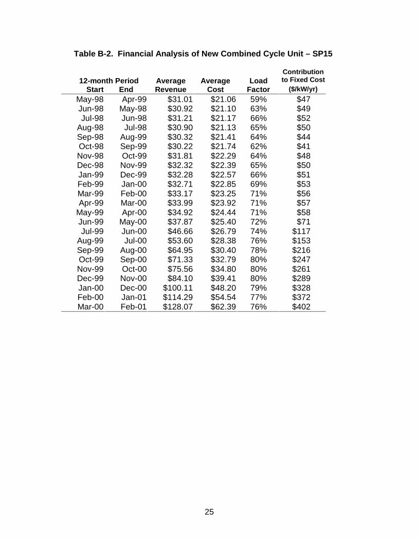
Table B-2. Financial Analysis of New Combined Cycle Unit – SP15

12-month Period Average Average LoadContributionto Fixed Cost

Start End Revenue Cost Factor ($/kW/yr)

May-98 Apr-99 $31.01 $21.06 59% $47Jun-98 May-98 $30.92 $21.10 63% $49Jul-98 Jun-98 $31.21 $21.17 66% $52

Aug-98 Jul-98 $30.90 $21.13 65% $50Sep-98 Aug-99 $30.32 $21.41 64% $44Oct-98 Sep-99 $30.22 $21.74 62% $41Nov-98 Oct-99 $31.81 $22.29 64% $48Dec-98 Nov-99 $32.32 $22.39 65% $50Jan-99 Dec-99 $32.28 $22.57 66% $51Feb-99 Jan-00 $32.71 $22.85 69% $53Mar-99 Feb-00 $33.17 $23.25 71% $56Apr-99 Mar-00 $33.99 $23.92 71% $57

May-99 Apr-00 $34.92 $24.44 71% $58Jun-99 May-00 $37.87 $25.40 72% $71Jul-99 Jun-00 $46.66 $26.79 74% $117

Aug-99 Jul-00 $53.60 $28.38 76% $153Sep-99 Aug-00 $64.95 $30.40 78% $216Oct-99 Sep-00 $71.33 $32.79 80% $247Nov-99 Oct-00 $75.56 $34.80 80% $261Dec-99 Nov-00 $84.10 $39.41 80% $289Jan-00 Dec-00 $100.11 $48.20 79% $328Feb-00 Jan-01 $114.29 $54.54 77% $372Mar-00 Feb-01 $128.07 $62.39 76% $402