STATE OF CALIFORNIA DEPARTMENT OF TRANSPORTATION TECHNICAL REPORT DOCUMENTATION PAGE TR0003 (REV. 10/98)

1. REPORT NUMBER CA14-2302

2. GOVERNMENT ASSOCIATION NUMBER

3. RECIPIENT’S CATALOG NUMBER

4. TITLE AND SUBTITLE

Develop a Plan to Collect Pedestrian Infrastructure and Volume Data for Future Incorporation into Caltrans Accident Surveillance and Analysis System Database

5. REPORT DATE

May 31, 2014 6. PERFORMING ORGANIZATION CODE

7. AUTHOR(S)

Yuanyuan Zhang, Frank R. Proulx, David R. Ragland, Robert J. Schneider, and Offer Grembek,

9. PERFORMING ORGANIZATION NAME AND ADDRESS

UC Berkeley Safe Transportation Research & Education Center 2614 Dwight Way, #7374 Berkeley, CA 94720-7374

10. WORK UNIT NUMBER

11. CONTRACT OR GRANT NUMBER

65N2302 12. SPONSORING AGENCY AND ADDRESS

California Department of Transportation Division of Research, Innovation and System Information, MS-83 1227 O Street Sacramento CA 95814

13. TYPE OF REPORT AND PERIOD COVERED Final report, 6-2012 to 5-2014 14. SPONSORING AGENCY CODE

15. SUPPLEMENTAL NOTES

16. ABSTRACT

This project evaluates the feasibility of developing a pedestrian and bicycle infrastructure database and volume database for the California state highway system. While Caltrans currently maintains such data for motor vehicles in the Traffic Accident Surveillance and Analysis System - Transportation System Network (TASAS-TSN) database, the agency does not keep records on pedestrian or bicycle facilities. This information is crucial for improving the safety of these vulnerable road users. This project developed a proposed database structure and corresponding data collection methodology. It is recommended that the databases be linked to TASAS using the connection ID instead of incorporating them directly into the existing database. The volume and infrastructure databases will be constructed separately to accommodate different data collection procedures. In particular, volume data should be updated more regularly than infrastructure data. Volume data must be collected during field visits either manually or using automated collection methods, while infrastructure data can be collected remotely using mapping services or in the field during field visits. The research team tested the structure and collection methodology by populating the database for 100 miles of state highway across two districts. Parallel to testing the consistency and integrity of the database, the team also generated a time-cost estimate for data collection for different facilities across the state highway system. The research team estimates that collecting the data in the field for the entire state highway system will require approximately 9,000 hours, while remote (computer-based) data collection will require about 4,000 hours. 17. KEY WORDS

TASAS, Pedestrian Volume, Infrastructure, database

18. DISTRIBUTION STATEMENT No restrictions. This document is available to the public through the National Technical Information Service, Springfield, VA 22161

19. SECURITY CLASSIFICATION (of this report)

Unclassified

20. NUMBER OF PAGES

110 21. PRICE N/A

Reproduction of completed page authorized

ADA Notice For individuals with sensory disabilities, this document is available in alternate formats. For information call (916) 654-6410 or TDD (916) 654-3880 or write Records and Forms Management, 1120 N Street, MS-89, Sacramento, CA 95814.

ii

DISCLAIMER STATEMENT

This document is disseminated in the interest of information exchange. The contents of this report reflect the views of the authors who are responsible for the facts and accuracy of the data presented herein. The contents do not necessarily reflect the official views or policies of the State of California or the Federal Highway Administration. This publication does not constitute a standard, specification or regulation. This report does not constitute an endorsement by the Department of any product described herein. For individuals with sensory disabilities, this document is available in alternate formats. For information, call (916) 654-8899, TTY 711, or write to California Department of Transportation, Division of Research, Innovation and System Information, MS-83, P.O. Box 942873, Sacramento, CA 94273-0001.

iii

DEVELOP A PLAN TO COLLECT PEDESTRIAN INFRASTRUCTURE AND

VOLUME DATA FOR FUTURE INCORPORATION INTO CALTRANS

ACCIDENT SURVEILLANCE AND ANALYSIS SYSTEM DATABASE

FINAL TECHNICAL REPORT

PREPARED BY THE UC BERKELEY SAFE TRANSPORTATION RESEARCH AND EDUCATION CENTER

FOR THE CALIFORNIA DEPARTMENT OF TRANSPORTATION

MAY 31, 2014

YUANYUAN ZHANG

FRANK PROULX DAVID RAGLAND

ROBERT SCHNEIDER OFFER GREMBEK

iv

ACKNOWLEDGEMENTS

The authors would like to thank the California Department of Transportation for their support of this project. We especially acknowledge the support and guidance of Fred Yazdan, Roya Hassas, Brian Alconcel, Dario Senor, Lucia Saavedra, Dean Samuelson, Johnny Bhullar, Vladimir Poroshin, Eric Wong, Hau Doan, Bruce De Terra, Tracy Frost, Darold Heikens, Chris Ratekin, Emilly Mraovich, Debbie Silva, and Mitchell Prevost from Caltrans Head Quarter. Thanks to Mai Lieu and Mike Pickford for testing the data collection process in District 4 and 11. We also appreciate the support and corporation of Ronald Au-Yeung, Beth Thomas, Ramiel Gutierrez, from District 4, and Chris Schmidt, from District 11. Nicole Foletta, Meghan Weir, and Meghan Mitman have all made valuable contributions to this work. The assistance and advice of Jill Cooper, Swati Pande, Grace Felschundneff, and Tony Dang are also greatly appreciated. This work couldn’t have been possible without the dedication and motivation of Yizhe Liu, Brandon Lee, Noor Al-samarrai, Sana Iqbal Ahmed, and Lilia Houshmand who conducted the data collection efforts.

v

TABLE OF CONTENTS EXECUTIVE SUMMARY 1 1 INTRODUCTION 2 2 INSTITUTIONAL PROCEDURES AND REQUIREMENTS FOR DATABASE

UPDATING 4 2.1 BACKGROUND 4 2.2 ORIGINS OF TASAS-TSN 4 2.3 DATABASE STRUCTURE 4 2.4 DATABASE UPDATE/MAINTENANCE PROCEDURES 6 2.5 LEGAL CONSIDERATIONS 7 2.6 CONCLUSIONS 7

3 BACKGROUND RESEARCH ON PEDESTRIAN INFRASTRUCTURE

INVENTORIES AND VOLUME MODELING 9 3.1 PEDESTRIAN INFRASTRUCTURE INVENTORIES 9 3.2 DATA COLLECTION PROCEDURES 13 3.3 POTENTIAL ITEMS TO INCLUDE IN PEDESTRIAN DATABASE 14 3.4 CONCLUSIONS 25

4 DATABASE STRUCTURE AND DESIGN 27 4.1 DECOMPOSITION OF A TYPICAL ROAD SEGMENT 27 4.2 COMPONENT DEFINITIONS AND CONNECTIONS 28 4.3 DATABASE STRUCTURE 31

5 DATA COLLECTION MANUAL 34 5.1 FACILITY DATA COLLECTION 35 5.2 VOLUME DATA COLLECTION 57

6 DATA COLLECTION PILOT 60 6.1 COMPUTER DATA COLLECTION 61 6.2 FIELD DATA COLLECTION 66 6.3 VOLUME DATA COLLECTION 67

7 TIME COST FOR DATA COLLECTION 72 7.1 COMPUTER DATA COLLECTION 73 7.2 FIELD DATA COLLECTION 74 7.3 COMPARISONS 75

8 CONCLUSIONS AND RECOMMENDATIONS 77

8.1 CONCLUSIONS 77 8.2 RECOMMENDATIONS 78

APPENDIX 1. Notes from Interview with Eric Fredericks, Caltrans District 3 81 APPENDIX 2. Notes from Interview with Darold Heikens, Caltrans ADA Infrastructure

Program Chief 83 APPENDIX 3. Notes from Interview with Debra Kingsland, New Jersey DOT Bike &

Pedestrian Program Section Chief 84 APPENDIX 4. User Testing and Comments 85 APPENDIX 5. Field Data Collection Packet 101 APPENDIX 6. Time-Estimation Spreadsheet Tool 105

1

EXECUTIVE SUMMARY In this report, a database format is proposed for storing pedestrian and bicycle infrastructure and volume data collected across the California state highway network. Data collection protocols are detailed for filling both databases. Additionally, a pilot data collection effort was conducted to verify that the data can be collected both via computer-based imagery and field-based collection. In the process of conducting the pilot data collection, the amount of time required was recorded and used to estimate the total time cost for collecting data across the entire state highway network. The database is comprised of two sub-databases, one for infrastructure and one for volumes. Both of these databases are structured around two “core elements”—nodes and approaches. These core elements give spatial structure to the database. Nodes are defined as including typical highway intersections and intersections between highways and cross streets, as well as mid-block crossings, pedestrian over/underpasses, and periodic locations along highways where a node has not otherwise been triggered. Approaches are simply defined as connecting nodes, with one approach for each direction of the highway. “Secondary elements” are then defined to represent pedestrian and bicycle infrastructure and volumes, which are linked to the core elements based on spatial location. For example, sidewalks are defined with reference to a single approach, whereas crosswalks are defined with reference to one node and two approaches. Using this framework, a number of secondary elements are defined for pedestrian infrastructure and volumes, including sidewalks, crosswalks, buffers (between the motor vehicle lane and sidewalk), and bicycle facilities, among others. For each of these elements, a number of attributes are defined. For example, crosswalk attributes include crossing distance, crosswalk design, crosswalk color, presence of detectable warning surfaces, presence and type of curb ramps, and other similar features. Data collection protocols for all of these elements are defined, including using Google maps/Google Street View and via field observation. The computer-based data collection procedures were tested on 100 miles of state highway, and a seven-mile subset of data was collected using field data collection. Of the 100 miles, fifty were chosen from Caltrans District 4, and fifty were chosen from District 11. In addition to verifying that the data collection process works as intended, the pilot was used to estimate a time cost for collecting this data across the entire state highway system. It is uncertain whether the database will eventually be merged into Caltrans’ Traffic Accident Surveillance and Analysis System (TASAS) - Transportation System Network (TSN), or whether it will be developed as a separate database with links to TASAS - TSN. Caltrans staff will need to make a decision about which option fits best within the existing technological framework.

2

1 INTRODUCTION This report documents California Strategic Highway Safety Plan (SHSP) Action Item 08.09: “Develop a Plan to Collect Pedestrian Infrastructure and Volume Data for Future Incorporation into Caltrans Accident Surveillance and Analysis System Database.” For this project, a relational database was developed to store information on pedestrian and bicycle infrastructure and volume. This database is designed to be linkable to the existing Caltrans Traffic Accident Surveillance and Analysis System (TASAS) - Transportation System Network (TSN) database, which includes information on California’s state highway system including infrastructure (e.g., number of lanes, lane widths, etc.), vehicular volumes, and crashes. However, the existing database does not include any information on pedestrian- and bicyclist-specific infrastructure, such as the presence of sidewalks or crosswalks, crossing distances, facility widths, etc.

In addition to designing the database, a data collection process to populate the database was developed and pilot tested across a subset of the state highway system. The data collection process was developed for both computer-based data collection and field-data collection. The pilot test encompassed 97.42 miles using the computer data collection method and 7.3 miles using the field data collection method. In addition to the pilot data collection conducted by the research team, two Caltrans staff members also tested the data collection protocols on small stretches of highway to ensure that the process aligns with their expert knowledge of the state highway system. The primary goals of this project are to (1) design a flexible database to store pedestrian and bicycle infrastructure and volume data to be queried in safety analyses, for network deficiencies, and any other uses; (2) to determine an efficient method of collecting data that can be scaled for use across the entire state highway system; (3) to pilot test the data collection process and ensure that all data can be feasibly collected and stored within the database framework; and (4) to estimate the total time-cost of collecting this data across the entire state highway system. Key Components The report is divided into eight chapters that describe the overall project and findings.

Chapter 1 includes an introduction that elaborates on the purpose and background of the project.

Chapter 2 details the institutional aspects of the existing TASAS-TSN database, including the origins of the database, maintenance procedures, and potential concerns about implementing new variables. The material presented in this chapter is based on a series of telephone interviews with various Caltrans staff. Chapter 3 presents a review of similar pedestrian and bicycle infrastructure inventories carried out in various cities and states. Many cities and a few states have conducted sidewalk inventories with varying levels of data detail collected. For example, some cities simply note the presence of sidewalks, whereas others use wheelchair-mounted sensors to collect detailed information on sidewalk quality conditions. Data collection procedures have included walking field inventories, review of state highway video logs, and review of still imagery. Chapter 3 also includes a review of literature on direct demand modeling for pedestrians based on transportation network and land use characteristics. This literature aims to estimate pedestrian volumes throughout the network, which is one potential use of the volume database component of this project.

3

Chapter 4 describes the database developed during this project to store pedestrian and bicycle infrastructure and volume data. The structure used is based on two core elements, nodes and approaches, which provide the spatial structure for the highway network. Nodes correspond to intersections, midblock crosswalks, and points every 1-mile along remote highways (i.e., whenever nodes do not occur for any other reason). Approaches refer to the connections between nodes. Approaches are defined by the direction of motor vehicle traffic, meaning that between two intersections (two nodes) on a bidirectional road, there are two approaches. Secondary elements such as sidewalks, crosswalks, buffer zones, and bicycle facilities are then each related by a unique ID to the approaches and nodes. Separate tables are used for each element type (e.g., approaches, nodes, sidewalks, crosswalks, buffers). Chapter 5 includes the Data Collection Manual, a document describing all of the data elements to be collected for this database in detail. Directions are given for taking different measurements and for classifying categorical information, such as crosswalk types. Chapter 6 describes the pilot data collection process and provides instructions for collecting data in the field. The pilot was conducted with the goals of refining the data collection process and database format, estimating the total time required to collect data across the entire state highway network, and checking the feasibility of collecting infrastructural data using remote imagery. The data collection pilot was conducted in Caltrans Districts 4 and 11 with support from local staff, and included user testing of the data collection process on a short set of highway segments by two Caltrans staff members. This user testing served as a peer review to ensure that professionals not immediately involved with developing the database would be able to follow the data collection procedures. Based on the results of the data collection pilot, Chapter 7 provides estimates of the time required for collection of pedestrian and bicycle infrastructural data across the entire California state highway network using various data collection processes (computer-based, field-based, and a hybrid approach). Cost estimates are not provided for populating the volume database. Volume data is proposed for collection as part of regular traffic safety investigations and other field visits, as the cost of installing a Miovision camera is very low. The volume data should be collected as frequently as is feasible. Finally, Chapter 8 presents conclusions and recommendations for implementation of the data collection process documented herein. Areas for future discussion include software for use in implementing the database, whether a GIS-based approach should be considered, connections to the existing TASAS-TSN system, and plans and a timeline for conducting the complete pedestrian and bicycle infrastructure inventory.

4

2 INSTITUTIONAL PROCEDURES AND REQUIREMENTS FOR DATABASE UPDATING

2.1 BACKGROUND This report summarizes the existing data contents and database management practices related to the TASAS-TSN database. Based on information gathered for this report from Caltrans, it may be more practical for pedestrian-related data to first be collected and stored in a database that is parallel to but separate from the existing TASAS-TSN database. These data could eventually be integrated into the existing system or a future system that incorporates a full set of multimodal data on the State Highway System, or kept as a standalone system alongside TASAS-TSN.

Background research for this report was conducted through meetings with Caltrans Transportation Systems Information Staff in fall 2011, a project kick-off meeting in spring 2012, a review of the current Caltrans Traffic Manual (http://www.dot.ca.gov/hq/traffops/engineering/ control-devices/trafficmanual-current.htm), and telephone interviews with other Caltrans headquarters and district staff in fall 2012. Notes from these meetings are attached to this document as appendices.

2.2 ORIGINS OF TASAS-TSN To the best of our knowledge, the original TASAS database was developed in the 1960s. The original data fields included automobile volumes and basic automobile infrastructure information, such as the number of lanes on the roadway, roadway configuration, and median and shoulder characteristics. All data fields in the current TASAS-TSN database were conveyed from the Legacy System, an earlier version of the TASAS database. New data fields have not been added since the database was first created.

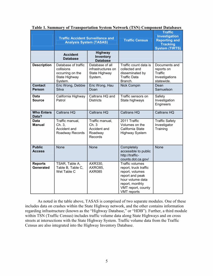
2.3 DATABASE STRUCTURE The TASAS database is currently stored as an Oracle 10g database. The official database is housed on servers at Caltrans headquarters in Sacramento. TASAS is a component of the larger Transportation System Network (TSN) database structure, which includes a number of modules with separate data themes, as shown in Table 1.

5

Table 1. Summary of Transportation System Network (TSN) Component Databases

Traffic Accident Surveillance and Analysis System (TASAS) Traffic Census

Traffic Investigation

Reporting and Tracking

System (TIRTS) Accident

Database Highway Inventory Database

Description Database of traffic collisions occurring on the State Highway System.

Database of all infrastructures on State Highway System.

Traffic count data is collected and disseminated by Traffic Data Branch.

Documents and reports on Traffic Investigations statewide.

Contact Person

Eric Wong, Debbie Silva

Eric Wong, Hau Doan

Nick Compin Dean Samuelson

Data Source

California Highway Patrol

Caltrans HQ and Districts

Traffic sensors on State highways

Safety Investigation Engineers

Who Enters Data?

Caltrans HQ Caltrans HQ Caltrans HQ Caltrans HQ

Data Manual

Traffic manual, Ch. 3, Accident and Roadway Records

Traffic manual, Ch. 3 Accident and Roadway Records

2011 Traffic Volumes on the California State Highway System

Traffic Safety Investigator Training

Public Access

None None Completely accessible to public http://traffic-counts.dot.ca.gov/

None

Reports Generated

TSAR, Table A, Table B, Table C, Wet Table C

AXR330, AXRO85, AXR085

Traffic volumes report, truck traffic report, volumes report and peak hour volume data report, monthly VMT report, county VMT reports

As noted in the table above, TASAS is comprised of two separate modules. One of these includes data on crashes within the State Highway network, and the other contains information regarding infrastructure (known as the “Highway Database,” or “HDB”). Further, a third module within TSN (Traffic Census) includes traffic volume data along State Highways and on cross streets at intersections with the State Highway System. Traffic volume data from the Traffic Census are also integrated into the Highway Inventory Database.

6

2.4 DATABASE UPDATE/MAINTENANCE PROCEDURES The TASAS Highway Database (HDB) contains information about segments (between intersections), intersections, and ramps. This database is jointly maintained by Caltrans headquarters and individual district offices. The TASAS-TSN database currently includes the following pedestrian-relevant data fields: Highway Database

Number of lanes Motor vehicle ADT Median type Median width Treated shoulder width Traveled way width

Intersection Database

Type (4-leg, T, Y) Control type (signal, stop) Lighting (Y or N) Channelized left-turn lane (Mainline & Cross) Channelized right-turn lane (Mainline & Cross) 1-way vs. 2-way traffic flow (Mainline & Cross) Number of lanes (Mainline & Cross)

Ramp Database

On vs. Off ramp Ramp type (diamond, loop, slip)

These existing data will not need to be collected as part of this project. However, it may

be advisable to add these existing values to the new pedestrian database for ease of use in analysis.

Infrastructure data updates are forwarded to Headquarters from Districts based on “As-Built” plans. There is currently no established procedure in place to collect measurements or other observations in the field to check, update, or expand the existing data. For example, if District 4 traffic investigators find any locations on the State Highway network that are inconsistent with the TASAS database, the district TASAS coordinator is notified, who in turn notifies Headquarters.

Based on correspondence with Caltrans staff, any modifications to the state highway system are recorded in a “masterlist.” Modifications come from different departments based on the nature of the change as follows:

Adoptions are reported by the Division of Design Constructed Projects are reported by the Division of Construction Project Completion Dates are reported by Project Management Relinquishments are reported by HQ Right of Way Any other known changes are reported by the districts

7

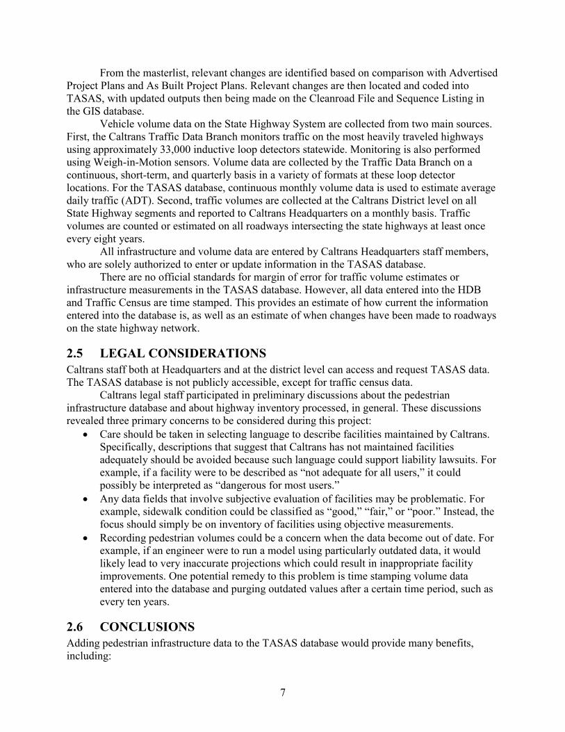
From the masterlist, relevant changes are identified based on comparison with Advertised Project Plans and As Built Project Plans. Relevant changes are then located and coded into TASAS, with updated outputs then being made on the Cleanroad File and Sequence Listing in the GIS database.

Vehicle volume data on the State Highway System are collected from two main sources. First, the Caltrans Traffic Data Branch monitors traffic on the most heavily traveled highways using approximately 33,000 inductive loop detectors statewide. Monitoring is also performed using Weigh-in-Motion sensors. Volume data are collected by the Traffic Data Branch on a continuous, short-term, and quarterly basis in a variety of formats at these loop detector locations. For the TASAS database, continuous monthly volume data is used to estimate average daily traffic (ADT). Second, traffic volumes are collected at the Caltrans District level on all State Highway segments and reported to Caltrans Headquarters on a monthly basis. Traffic volumes are counted or estimated on all roadways intersecting the state highways at least once every eight years.

All infrastructure and volume data are entered by Caltrans Headquarters staff members, who are solely authorized to enter or update information in the TASAS database.

There are no official standards for margin of error for traffic volume estimates or infrastructure measurements in the TASAS database. However, all data entered into the HDB and Traffic Census are time stamped. This provides an estimate of how current the information entered into the database is, as well as an estimate of when changes have been made to roadways on the state highway network.

2.5 LEGAL CONSIDERATIONS Caltrans staff both at Headquarters and at the district level can access and request TASAS data. The TASAS database is not publicly accessible, except for traffic census data.

Caltrans legal staff participated in preliminary discussions about the pedestrian infrastructure database and about highway inventory processed, in general. These discussions revealed three primary concerns to be considered during this project:

Care should be taken in selecting language to describe facilities maintained by Caltrans. Specifically, descriptions that suggest that Caltrans has not maintained facilities adequately should be avoided because such language could support liability lawsuits. For example, if a facility were to be described as “not adequate for all users,” it could possibly be interpreted as “dangerous for most users.”

Any data fields that involve subjective evaluation of facilities may be problematic. For example, sidewalk condition could be classified as “good,” “fair,” or “poor.” Instead, the focus should simply be on inventory of facilities using objective measurements.

Recording pedestrian volumes could be a concern when the data become out of date. For example, if an engineer were to run a model using particularly outdated data, it would likely lead to very inaccurate projections which could result in inappropriate facility improvements. One potential remedy to this problem is time stamping volume data entered into the database and purging outdated values after a certain time period, such as every ten years.

2.6 CONCLUSIONS Adding pedestrian infrastructure data to the TASAS database would provide many benefits, including:

8

Making more data available to address pedestrian safety issues. Pedestrians currently represent approximately 20% of fatalities in California.

Providing data to monitor, analyze, and plan for a multimodal transportation system. Deputy Directive 64-R1 emphasizes that pedestrian needs will be integrated into all aspects of Caltrans policies, planning, and project delivery.

Establishing baseline data to document pedestrian infrastructure gaps and other pedestrian safety needs. The baseline data can be tracked to show how many pedestrian improvements Caltrans has made over time.

Gathering data on pedestrian infrastructure characteristics and pedestrian volumes in a statewide database to provide a more complete picture of pedestrian risk. This can illustrate the types of roadways and geographic locations with the greatest need for pedestrian safety countermeasures.

Providing data for before and after evaluations and other system analyses that can produce new pedestrian crash modification factors (CMFs). Better pedestrian CMFs will lead to more effective pedestrian crash countermeasures that can be applied after traffic safety investigations.

There are also several overall challenges associated with adding new pedestrian data to

the TASAS database, which should be considered while moving forward with this project. These include:

Legal issues related to the new data (e.g., using care in language choice, collecting objective data, keeping information up-to-date). It will be important for the project team to continue to coordinate with Caltrans Legal staff as the project moves forward.

Adding new fields within existing TASAS database may change coding used to produce automatic reports (e.g., Table C). This is one reason why the additional pedestrian data fields could be kept in a separate database before considering the possibility of integrating them into a future TASAS database format.

District TASAS coordinators would also send pedestrian infrastructure updates. This will require additional awareness and possibly more training.

Federal funding is currently tied to motor vehicle volume reporting, not pedestrian and bicycle volume reporting. Additional time spent collecting pedestrian and bicycle volume data could consume resources that are currently used to obtain this federal funding. However, federal requirements for volume data reporting may become multimodal in the future.

The information gathered in Task 1 will provide a background foundation for future

tasks. Ultimately, the final Data Plan Report will recommend the most efficient data collection approach for integrating pedestrian data into the statewide TASAS-TSN database.

9

3 BACKGROUND RESEARCH ON PEDESTRIAN INFRASTRUCTURE INVENTORIES AND VOLUME MODELING

This project recommends that pedestrian infrastructure and volume data fields be added to the Caltrans transportation system information database. This involves developing a database structure, collecting data on the State Highway System, integrating the pedestrian data with all other transportation system variables, and maintaining the data over time. Similar efforts have been undertaken by other agencies, and lessons learned from these experiences can help form the process of updating Caltrans’ State Highway System database. This document presents background research on two main topics: 1) pedestrian infrastructure inventories, and 2) pedestrian volume models. The example inventories and models are from both California and other parts of North America.

Ultimately, new pedestrian data fields can form the foundation of a database including pedestrian crash, pedestrian exposure, and detailed pedestrian infrastructure information. Combining these three main types of data makes it possible to track pedestrian crash risk over time, analyze roadway features associated with pedestrian crash risk, develop pedestrian crash modification factors, and conduct other useful analyses. This rich set of information will help Caltrans select the most effective engineering, education, and enforcement treatments to reduce pedestrian injuries on the State Highway System and other roadways in California.

3.1 PEDESTRIAN INFRASTRUCTURE INVENTORIES This section summarizes several successful pedestrian infrastructure inventories conducted by agencies at the state, county, and city levels. The description of each inventory includes the data fields collected, as well as the year of collection, size of the network, data collection method, and reported costs of data collection, wherever available. Based on this review, a list of potential data fields for inclusion in the Caltrans pedestrian infrastructure inventory are itemized, as well as a brief assessment of the importance of collection and potential methods for collecting the data.

3.1.1 STATE DOT EFFORTS Caltrans has not coordinated a pedestrian infrastructure inventory at the state level, however District 3 developed a Complete Streets inventory database for all State Highways in the Sacramento region. This effort illustrates some of the pedestrian- and bicycle-related fields that could be collected for the entire State Highway System. Specific data fields can be found online at: <http://www.dot.ca.gov/dist3/departments/planning/communityplanning1.htm>. Examples of these fields include the presence of sidewalks, pedestrian-scale street lighting, marked pedestrian crossings, median islands, and curb extensions. Appendix 1 lists some of the important lessons learned by District 3 during the inventory process. A related Caltrans effort took place within the ADA Infrastructure Program, which included inventory of non-ADA compliant pedestrian infrastructure along the State Highway System. Non-compliant facilities are geo-referenced, and details pertaining to which features of the facility are non-compliant and how far outside of the acceptable range are included in this inventory. Data was collected through field inventory, and was recorded both using paper spreadsheets which were later input to computer spreadsheets, as well as tablet computers which offer the benefit of automatically geo-referencing records. This database will be integrated into the CT Earth architecture. The data is used in prioritization of facility improvements to meet

10

ADA requirements at the District level. Appendix 2 provides additional notes on the Caltrans ADA inventory.

Caltrans has also developed several documents that recommend specific pedestrian infrastructure elements to include as a part of planning, design, and engineering efforts. [Placeholder for ADA & Complete Streets Asset Management TSI form; Transportation Concept Report (TCR) System Planning Guidelines; Appendix S: Planning Scoping Information Sheet; SHOPP Program Reporting Form]

Other state DOTs have created statewide pedestrian infrastructure inventory databases (Table 2). However, these inventories each focus on a slightly different set of pedestrian facilities and do not include pedestrian volume or pedestrian risk estimates. Examples of similar projects to the proposed Caltrans State Highway System pedestrian database are discussed below: Washington1: WSDOT records video of approximately half of their state highways annually using a van with special video equipment, including date of recording. To create an inventory of pedestrian infrastructure, this video footage was reviewed by analysts who recorded data on sidewalks, marked crosswalks, and other pedestrian and bicycle facilities. The inventory was then field-checked by driving along a number of the highways. New bicycle and pedestrian infrastructure is monitored through project control forms, and subsequently added to the inventory. WSDOT anticipates renewing the inventory every three to four years. Total costs of completing the 7,000-mile inventory (not including driving and video recording) are estimated at 700 hours for video analysis and 1,000 hours for field checking. It should be noted that Caltrans also has a video log that could be viewed to determine whether a particular state highway segment has sidewalks or other visible pedestrian facilities, but features from the video log have not been entered into a database. New Jersey2: NJDOT has constructed an inventory of pedestrian and bicycle infrastructure presence along all county roads in the state, a total of approximately 13,200 miles. Data were collected using a vehicle equipped with GPS and four digital cameras. The imagery was then analyzed and compiled into a database, noting the presence of pedestrian and bicycle facilities. All data is available for download by county both as PDF maps and in GIS data formats. Appendix 3 includes additional lessons learned from NJDOT. Maryland3: The Maryland State Highway Administration (SHA) performed a sidewalk inventory focusing on ADA compliance. Data was collected in the field using GPS. A total of 874 miles of sidewalk were studied, and ADA compliance was checked for sidewalks, bus stops, curb ramps, driveway crossings, and median treatments.

1 Washington State DOT. Statewide Bicycle and Pedestrian Facility Inventory. <http://www.wsdot.wa.gov/NR/rdonlyres/3FBE90E2-77C7-4895-8D8D-81D251C7AF47/0/Inventory.pdf>. 2 New Jersey State DOT. County Road Sidewalk Inventory. October 2008. <http://www.state.nj.us/transportation/refdata/countysidewalks/>. 3 Maryland State Highway Administration. ADA Self Evaluation of Access to Public Right of Way Facilities. May 2009. <http://www.sha.maryland.gov/opr/ada%20self%20evaluation%205-09%20final.pdf>.

11

Table 2. Example State DOT Pedestrian Inventories

3.1.2 LOCAL JURISDICTIONAL EFFORTS Many of cities have conducted sidewalk inventories, some of which are presented below in Table 3, with several cases discussed in further detail. Rancho Cucamonga, CA4: The city of Rancho Cucamonga commissioned Vanderhawk Consulting LLC to conduct a sidewalk inventory. This inventory ranks missing sidewalk segment priority based on proximity to key pedestrian locations, such as schools, libraries, and shopping malls. Berkeley, CA5: The City of Berkeley’s Pedestrian Master Plan includes a thorough pedestrian network inventory. Data was collected by reviewing video imagery, examining city records, and conducting field spot-checks. Data collected is summarized in Table 3. The plan also prioritizes pedestrian infrastructure projects. Alexandria, VA6: The City of Alexandria’s Pedestrian and Bicycle Mobility Plan included an extensive inventory of bicycle and pedestrian infrastructure. Mobile GPS units were used to identify the locations of specific features such as curb ramps and sidewalk obstructions. Facility improvements were prioritized based on existing conditions as well as anticipated demand, estimated crash risks, and public input. Sacramento County, CA7: As part of the Sacramento County Master Plan process, a thorough pedestrian facilities inventory was collected along approximately 2,200 miles of streets and roadways in the county. The inventory includes data on sidewalk presence, intersection and street corner measurements and details, mid-block crossings, bike lane presence, parking type, 4 Vanderhawk Consulting LLC. Rancho Cucamonga Sidewalk Inventory Study. February 2011.< http://vanderhawk.net/2011/02/rancho-cucamonga-sidewalk-inventory/>. 5 City of Berkeley. Berkeley Pedestrian Master Plan. January 2010. <http://www.ci.berkeley.ca.us/pedestrian/>. 6 City of Alexandria, VA. City of Alexandria Pedestrian and Bicycle Mobility Plan. June 2008. < http://alexandriava.gov/localmotion/info/default.aspx?id=11418>. 7 County of Sacramento Department of Transportation. Sacramento County Pedestrian Master Plan. April 2007. <http://www.msa2.saccounty.net/transportation/Documents/SAC_PED_PLAN_FINAL__042807_Small.pdf>.

Inventory Year Collected Data Recorded Size of

System Reported

Costs Washington State DOT

2002-2003

Bike lanes, shoulders, shared-used pathways beside the roadway, sidewalks, walking paths (not worn dirt paths), signalized and un-signalized intersections, roadway medians, marked crosswalks, transit stops, and ADA facilities

7,000 miles

1700 total hours (700 for video analysis, 1,000 for field checking)

New Jersey DOT

2006-2007

Paths (sidewalks, shared use paths, and worn paths), bicycle lanes and routes, shoulders, crosswalks, curb ramps, pedestrian/bicycle related signage, pedestrian provisions at intersections (e.g. push-buttons and pedestrian signal heads)

13,200 miles

Not given

Maryland 2008-2009

ADA Compliance of sidewalks, bus stops, curb ramps, driveway crossings, and median treatments

874 sidewalk miles

Not given

12

posted speed limit, sidewalk conditions, traffic direction (if one-way), tree spacing in buffer, width of buffer, width of sidewalk, and width of pavement. The inventory was driven in part by a Pedestrian Level of Service (LOS) measure, which was used to rank the existing facilities. High-priority projects throughout the county are shown on maps, including project categories of signal timings, countdown signals, lighting, trail crossings, midblock crossings, pedestrian districts, sidewalks/asphalt walkways, alley conversions, and pathways.

Table 3. Example Local Jurisdiction Pedestrian Inventories

City Year Data Collected Size of Network

Data Collection Method

Rancho Cucamonga, CA

2011 Street name and from/to limits; Sidewalk presence; Street light presence; MicroPAVER section ID; Calculated length; Estimated width; Estimated surface area (can also be used for GASB 34); Location Type (e.g. hospital, library, school) Location Proximity- 500’, 1000′, and 1500′ buffers created around key locations; Reason(s) for missing sidewalk; Installation Priority Ranking

Unknown Aerial photography analysis

Berkeley, CA 2009 Sidewalk presence, sidewalk width, buffer width, sidewalk condition, marked crosswalk presence, crosswalk color, crosswalk condition, crosswalk marking type, crosswalk width, curb ramp presence, curb ramp type, curb ramp direction, truncated dome presence, separated pathways, pedestrian signal features

400 sidewalk miles

Video imagery, city records, field verification

Sacramento County, CA

2007 Sidewalk presence, intersection and street corner measurements and details, mid-block crossings, bike lane presence, parking type, posted speed limit, sidewalk conditions, traffic direction (if one-way), tree spacing in buffer, width of buffer, width of sidewalk, width of pavement

2,200 street/road miles

Field inventory

Oakland, CA8

2007 Sidewalk damage (type and degree), trees and tree wells, land use, ADA barriers, parking restrictions (curb markings), curb/gutter damage, signs, bus stops

Unknown Field inventory

Marina, CA9 2003 Pedestrian and bicycle facility deficiencies reported

Unknown

8 City of Oakland, CA. Streets & Sidewalks webpage. <http://www2.oaklandnet.com/Government/o/PWA/o/EC/s/STS/index.htm>. 9 Local Government Commission. Marina Pedestrian and Bicycle Master Plan. January 2004. <http://www.lgc.org/reports/marina/index.html>.

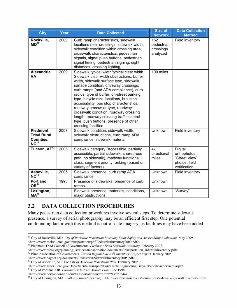
13

City Year Data Collected Size of Network

Data Collection Method

Rockville, MD10

2009 Curb ramp characteristics, sidewalk locations near crossings, sidewalk width, sidewalk condition within crossing area, crosswalk characteristics, pedestrian signals, signal push buttons, pedestrian signal timing, pedestrian signing, sight distances, crossing lighting,

162 pedestrian crossings analyzed

Field inventory

Alexandria, VA

2009 Sidewalk typical width/typical clear width, Sidewalk clear width obstructions, buffer width, sidewalk surface type, sidewalk surface condition, driveway crossings, curb ramps (and ADA compliance), curb radius, type of buffer, on-street parking type, bicycle rack locations, bus stop accessibility, bus stop characteristics, roadway crosswalk type, roadway crosswalk condition, roadway crossing length, roadway crossing traffic control type, push buttons, presence of other crossing facilities

100 miles

Piedmont Triad Rural Counties, NC11

2007 Sidewalk condition, sidewalk width, sidewalk obstructions, curb ramp ADA compliance, sidewalk material,

Unknown Field inventory

Tucson, AZ12 2005 Sidewalk category (Accessible, partially accessible, partial sidewalk, shared-use path, no sidewalk), roadway functional class, segment priority ranking (based on variety of factors)

4k directional miles

Digital orthophotos, “Street View” photos, field verification

Asheville, NC13

2005 Sidewalk presence, curb ramp ADA compliance

Unknown Field inventory

Portland, OR14

1998 Presence of sidewalks, presence of curb ramps

Unknown

Lexington, MA15

Sidewalk presence, materials, conditions, major obstructions

Unknown “Survey”

3.2 DATA COLLECTION PROCEDURES Many pedestrian data collection procedures involve several steps. To determine sidewalk presence, a survey of aerial photography may be an efficient first step. One potential confounding factor with this method is out-of-date imagery, as facilities may have been added

10 City of Rockville, MD. City of Rockville Pedestrian Inventory Study Safety and Accessibility Evaluation. May 2009. <http://www.rockvillemd.gov/transportation/pdf/PedestrianInventory2009.pdf>. 11 Piedmont Triad Council of Governments. Piedmont Triad Sidewalk Inventory. February 2007. <http://www.ptcog.org/planning_services/transportation/documents/transportation_sidewalkinventory.pdf>. 12 Pima Association of Governments. Tucson Region Sidewalk Inventory Project Report. January 2005. <http://www.pagnet.org/documents/Pedestrian/SidewalkInventory2005.pdf>. 13 City of Asheville, NC. The City of Asheville Pedestrian Plan. February 2005. <http://www.ashevillenc.gov/Departments/Transportation/TrafficEngineering/BicyclePedestrianServices.aspx>. 14 City of Portland, OR. Portland Pedestrian Master Plan. June 1998. <http://www.portlandonline.com/transportation/index.cfm?&a=90244>. 15 City of Lexington, MA. Walkway Inventory Group. < http://ci.lexington.ma.us/committees/sidewalk/sidewalkinventory.cfm>.

14

(or removed) since the photos were taken. However, such imagery is much more efficient for initial data collection than collecting measurements in the field, especially for rural areas and grade-separated highways (where pedestrian facilities are less common). As a second step, several data collection methods are available, depending on data fields desired. If Caltrans is particularly interested in the presence of median islands and sidewalk width, these observations and measurements can be made from aerial photography. If Caltrans is interested in documenting sidewalk obstructions, noting the presence of curb ramps, or identifying pedestrian countdown signals, observations might be made using video (as in Washington), still photos (as in New Jersey), or using Google Street View imagery. Finally, field data collection may be necessary for items such as sidewalk condition or pedestrian signal timing. For all types of data, field verification checks are advisable. If widths are measured using aerial imagery, and these are found to be systematically above or below ground truth values, measurements can be adjusted accordingly.

3.3 POTENTIAL ITEMS TO INCLUDE IN PEDESTRIAN DATABASE The following data items might be suitable for inclusion in the pedestrian infrastructure inventory. Depending on overall costs (to be determined in Tasks 3 and 4), items may be added or removed as necessary. This section describes why it is valuable to include specific infrastructure and volume (exposure) fields in Caltrans data systems, and specifies factors that are used in the calculation of Pedestrian Level of Service (LOS) in the Highway Capacity Manual with a “†” symbol.

3.3.1 SEGMENT DATA Sidewalk presence†—All inventories reviewed have included sidewalk presence as a feature, as it can be determined reliably using aerial photography. Sidewalks are important facilities for providing pedestrian accessibility. Walking on sidewalks is generally much safer for pedestrians than walking along roadways without sidewalks.16 Additionally, roadway segments with sidewalks along both sides of the road experience lower rates of pedestrian crashes than segments with sidewalks along only one side.17 Sidewalk width†—Adequate width is required for ADA compliance. Width is also important in determining whether there is sufficient sidewalk space for the pedestrian volumes present, akin to considerations of number of lanes for vehicle traffic. Wider sidewalks provide more lateral separation between pedestrians and moving vehicle traffic. One disadvantage of this characteristic is that it takes longer to measure sidewalk width than simply note sidewalk presence.

16 San Francisco Municipal Transportation Authority and University of California Traffic Safety Center, San Francisco PedSafe Phase II Final Implementation Report, FHWA Cooperative Agreement (Federal Highway Administration, February 2008); University of Florida Department of Civil and Coastal Engineering et al., Miami-Dade Pedestrian Safety Project: Phase II Final Implementation Report, FHWA Cooperative Agreement (Federal Highway Administration, August 2008); Shashi Nambisan, Mukund Dangeti, and Vinod Vasudevan, Pedestrian Safety Engineering and Intelligent Transportation System-Based Countermeasures Program For Reducing Pedestrian Fatalities, Injuries, Conflicts, and Other Surrogate Measures, Phase 2 Final Technical Report, September 15, 2008. 17 San Francisco Municipal Transportation Authority and University of California Traffic Safety Center, San Francisco PedSafe.

15

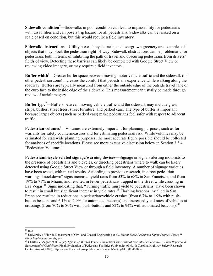
Sidewalk condition†—Sidewalks in poor condition can lead to impassability for pedestrians with disabilities and can pose a trip hazard for all pedestrians. Sidewalks can be ranked on a scale based on condition, but this would require a field inventory. Sidewalk obstructions—Utility boxes, bicycle racks, and overgrown greenery are examples of objects that may block the pedestrian right-of-way. Sidewalk obstructions can be problematic for pedestrians both in terms of inhibiting the path of travel and obscuring pedestrians from drivers’ fields of view. Detecting these barriers can likely be completed with Google Street View or reviewing video imagery, or may require a field inventory. Buffer width†—Greater buffer space between moving motor vehicle traffic and the sidewalk (or other pedestrian zone) increases the comfort that pedestrians experience while walking along the roadway. Buffers are typically measured from either the outside edge of the outside travel lane or the curb face to the inside edge of the sidewalk. This measurement can usually be made through review of aerial imagery. Buffer type†—Buffers between moving vehicle traffic and the sidewalk may include grass strips, bushes, street trees, street furniture, and parked cars. The type of buffer is important because larger objects (such as parked cars) make pedestrians feel safer with respect to adjacent traffic. Pedestrian volumes†—Volumes are extremely important for planning purposes, such as for warrants for safety countermeasures and for estimating pedestrian risk. While volumes may be estimated for statewide planning purposes, the most accurate figure possible should be collected for analyses of specific locations. Please see more extensive discussion below in Section 3.3.4. “Pedestrian Volumes.” Pedestrian/bicycle related signage/warning devices—Signage or signals alerting motorists to the presence of pedestrians and bicycles, or directing pedestrians where to walk can be likely detected using Google Street View or through a field inventory. A number of signage varieties have been tested, with mixed results. According to previous research, in-street pedestrian warning “knockdown” signs increased yield rates from 53% to 68% in San Francisco, and from 19% to 71% in Miami, and resulted in fewer pedestrians trapped in the street while crossing in Las Vegas.18 Signs indicating that, “Turning traffic must yield to pedestrians” have been shown to result in small but significant increase in yield rates.19 Flashing beacons installed in San Francisco resulted in reductions in pedestrian/vehicle crashes (from 6.7% to 1.9% with push-button beacons and 6.1% to 2.9% for automated beacons) and increased yield rates of vehicles at crossings (from 70% to 80% with push-buttons and 82% to 94% with automated beacons).20

18 Ibid. 19 University of Florida Department of Civil and Coastal Engineering et al., Miami-Dade Pedestrian Safety Project: Phase II Final Implementation Report. 20 Charles V. Zegeer et al., Safety Effects of Marked Versus Unmarked Crosswalks at Uncontrolled Locations: Final Report and Recommended Guidelines, Final, Evaluation of Pedestrian Facilities (University of North Carolina Highway Safety Research Center, August 2005), http://www.fhwa.dot.gov/publications/research/safety/04100/04100.pdf.

16

Rectangular Rapid Flashing Beacons (RRFBs) installed on two high-speed multilane arterials in Miami led to increased yield rates (from 0% to 65% and from 1% to 92%).21 Presence of transit stops—Most transit users travel to transit stops as pedestrians. Information on transit stops may be available via online aerial imagery (Google Maps), or using in street-level imagery.

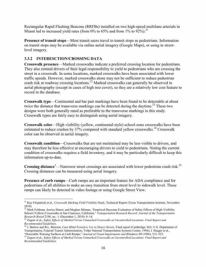
3.3.2 INTERESCTION/CROSSING DATA Crosswalk presence—Marked crosswalks indicate a preferred crossing location for pedestrians. They also remind drivers of their legal responsibility to yield to pedestrians who are crossing the street in a crosswalk. In some locations, marked crosswalks have been associated with lower traffic speeds. However, marked crosswalks alone may not be sufficient to reduce pedestrian crash risk at roadway crossing locations.22 Marked crosswalks can generally be observed in aerial photography (except in cases of high tree cover), so they are a relatively low cost feature to record in the database. Crosswalk type—Continental and bar pair markings have been found to be detectable at about twice the distance that transverse markings can be detected during the daytime.23 These two designs were both generally rated as preferable to the transverse markings in this study. Crosswalk types are fairly easy to distinguish using aerial imagery. Crosswalk color—High visibility (yellow, continental-style) school-zone crosswalks have been estimated to reduce crashes by 37% compared with standard yellow crosswalks.24 Crosswalk color can be observed in aerial imagery. Crosswalk condition—Crosswalks that are not maintained may be less visible to drivers, and may therefore be less effective at encouraging drivers to yield to pedestrians. Noting the current condition of crosswalks requires a field inventory, and it may be particularly difficult to keep this information up-to-date. Crossing distance†—Narrower street crossings are associated with lower pedestrian crash risk.25 Crossing distances can be measured using aerial imagery. Presence of curb ramps—Curb ramps are an important feature for ADA compliance and for pedestrians of all abilities to make an easy transition from street level to sidewalk level. These ramps can likely be detected in video footage or using Google Street View.

21 Kay Fitzpatrick et al., Crosswalk Marking Field Visibility Study, Technical Report (Texas Transportation Institute, November 2010). 22 Mark Feldman, Jessica Manzi, and Meghan Mitman, “Empirical Bayesian Evaluation of Safety Effects of High-Visibility School (Yellow) Crosswalks in San Francisco, California,” Transportation Research Record: Journal of the Transportation Research Board 2198, no. -1 (December 1, 2010): 8–14. 23 Zegeer et al., Safety Effects of Marked Versus Unmarked Crosswalks at Uncontrolled Locations: Final Report and Recommended Guidelines. 24 J. Barlow and B.L. Bentzen, Cues Blind Travelers Use to Detect Streets, Final report (Cambridge, MA: U.S. Department of Transportation, Federatl Transit Administration, Volpe National Transportation Systems Center, 1994); J. Hauger et al., “Detectable Warning Surfaces at Curb Ramps,” Journal of Visual Impairments and Blindness 90 (1996): 512–525. 25 Zegeer et al., Safety Effects of Marked Versus Unmarked Crosswalks at Uncontrolled Locations: Final Report and Recommended Guidelines.

17

Presence of truncated domes—Truncated domes serve as a warning device for vision-impaired pedestrians at crossing locations. Visually impaired pedestrians are often unable to detect the edge of a street when a curb ramp is present without truncated domes, as their key signifier of a street is the down curb.26 Truncated domes can generally be seen in aerial imagery, or in street-level imagery. Number of lanes to cross—Multilane roadways are less safe and feel less comfortable for pedestrians to cross than two-lane roadways. Multilane roadways create a multiple threat situation for pedestrians: a vehicle in one lane may stop for a pedestrian in a crosswalk, but a vehicle in the next lane may not see the pedestrian. The number of lanes is visible in aerial imagery, based on lane markings. Pedestrian signal heads†—Pedestrian crossing signals have been shown to reduce pedestrian crash risk at high volume intersections.27 Some signal heads are equipped with countdown timers to let pedestrians know how much time remains before the “Do Not Walk” signal phase. The presence of this feature might be difficult to determine, potentially requiring field visits. In one study, pedestrian countdown timers were not found to significantly decrease pedestrian/vehicle crashes, but were associated with a significant decrease in all crashes, possibly due to drivers utilizing the countdown timer to determine how much time remains before the red light phase.28 In Miami, countdown signals were shown to correspond to higher rates of pedestrians pushing signal actuator buttons.29 In San Francisco, countdown signals were found to result in a lower number of pedestrians crossing during the red phase (reduction from 14% to 9%), a 22% reduction in pedestrian injury crashes, and a reduction in the percentage of all traffic crashes caused by drivers running red lights from 45% to 34%.30 Pedestrian signal heads may be possible to inventory from street-level images. Pedestrian signal actuator buttons—Pedestrian push-buttons are needed at some traffic signal locations to include a pedestrian crossing interval in the traffic signal cycle. These buttons are also an important component of many accessible pedestrian signals. These buttons can likely be inventoried using street-level imagery. Pedestrian volumes†—See argument given in sub-section “Segment Data.” Median passable—Determining whether street medians are passable for pedestrian is important in identifying accessible mid-block crossings. Median (and sidewalk) barriers can be used to channelize pedestrians into specific crossing locations.31 This data can be found using street level imagery. 26 Srinivas S. Pulugurtha, Arpan Desai, and Nagasujana M. Pulugurtha, “Are Pedestrian Countdown Signals Effective in Reducing Crashes?,” Traffic Injury Prevention 11, no. 6 (2010): 632–641. 27 University of Florida Department of Civil and Coastal Engineering et al., Miami-Dade Pedestrian Safety Project: Phase II Final Implementation Report. 28 San Francisco Municipal Transportation Authority and University of California Traffic Safety Center, San Francisco PedSafe. 29 Biotechnology Inc. et al., Urban Pedestrian Accident Countermeasures Experimental Evaluation (BioTechnology, 1975). 30 Mighk Wilson and Theodore A. Petritsch, “Quantifying Countermeasure Effectiveness - Orlando, FL” (Pedestrian and Bicycle Information Center, 2008), www.walkinginfo.org. 31 San Francisco Municipal Transportation Authority and University of California Traffic Safety Center, San Francisco PedSafe.

18

Presence of median refuge—Crossing arterials (6 lanes) without medians has been found to be 6.5 times more risky than crossing arterials with medians.32 In San Francisco, 70% of pedestrians reported feeling safer crossing streets with median refuges.33 Median refuges both shorten the crossing distance and simplify the crossing task by only requiring the pedestrian to focus on unidirectional traffic. Median refuges at midblock locations have also been shown to increase driver yielding rates and to decrease pedestrian delay.34 They are especially important on wide (4+ lane) roads. Median refuges can likely be seen in aerial imagery. It will probably not be feasible to include all of the above items in the database due to cost constraints and/or legal considerations. Accordingly, they have been approximately sorted into three categories shown below: low, medium, and high cost. Costs for each data field have been roughly approximated based solely on potential collection technique (noted in parentheses), and have been evaluated for optimization regarding both cost and relative importance. These data collection options and associated costs will be developed more formally in Task 3 Low Cost (Aerial Imagery)

Sidewalk presence Buffer presence Marked crosswalk presence Crosswalk type Median refuge presence Pedestrian volumes35

Medium Cost (Street-level imagery; Google Street View; Video log)

All of the above, plus: Curb ramp presence Truncated domes presence Pedestrian/bicycle related signage Sidewalk width Buffer width and type Crossing distance Sidewalk obstructions Median refuge width and accessibility Pedestrian signal heads Pedestrian signal actuator buttons Crosswalk color

32 David Harkey and Charles Zegeer, “PEDSAFE: Pedestrian Safety Guide and Countermeasure Selection System,” FHWA Report FHWA-SA-04-003, 2004. < http://www.walkinginfo.org/training/collateral/resources/PEDSAFEGuide.pdf>. 33 Pedestrian volumes will not be a low cost piece of data to collect. However, they are extremely important for a variety of applications, and hence should be estimated in even the lowest cost database. 34 S. Pulugurtha and S. Repaka, “Assessment of Models to Measure Pedestrian Activity at Signalized Intersections,” Transportation Research Record: Journal of the Transportation Research Board, vol. 2073, no. -1, pp. 39–48, Dec. 2008. 35 R. Schneider, L. Arnold, and D. Ragland, “Pilot Model for Estimating Pedestrian Intersection Crossing Volumes,” Transportation Research Record: Journal of the Transportation Research Board, vol. 2140, no. -1, pp. 13–26, Dec. 2009.

19

High Cost (Field Inventory) All of the above, plus: Sidewalk condition Crosswalk condition Presence of transit stops

3.3.3 EXTENSION TO INCLUDE BICYCLE INFRASTRUCTURE As a part of background discussions to provide information for Task 1 and Task 2, several members of Caltrans and the project team mentioned that it would be worth exploring the possibility of adding bicycle infrastructure in the TASAS database in addition to pedestrian infrastructure. This has been scoped as a pedestrian project, but there would be several advantages to including basic bicycle infrastructure items (e.g., presence of bicycle lanes, width of bicycle lanes, width of paved shoulder, bicycle route signs, and multi-use trails adjacent to State Highways), including the following:

To fully achieve the policy established through Deputy Directive 64-R1, which is to include all modes (such as pedestrian and bicycle) in all aspects of Caltrans planning and operations.

To provide data that can be used to analyze how well State Highways serve as “Complete Streets.”

To allow bicycle data to be collected at a much lower cost than if the data were collected in a separate project (e.g., if data collectors are collecting sidewalk and other pedestrian infrastructure for a particular State Highway segment or intersection, they can note relatively quickly whether or not bicycle lanes and other bicycle infrastructure are present).

3.3.4 PEDESTRIAN VOLUMES Pedestrian volume data are an important element for inclusion in the Caltrans State Highway System information database. They should be provided for intersections (e.g., total count of pedestrians crossing each leg of the intersection during a specific time period) as well as along roadway segments (e.g., total count of pedestrians passing the midpoint of a roadway segment during a specific time period). Volumes are necessary to estimate the relative risk of pedestrian crashes for individuals traveling along state highways (i.e., pedestrian crashes/pedestrian volume). Identifying locations that have higher relative pedestrian risk can indicate which roadway design features or other characteristics should be modified to reduce pedestrian crashes and injuries. Volume data can also be used to determine how common pedestrian activity is on the State Highway System, showing the importance of designing roadways for safe and convenient pedestrian access.

However, it is impractical to count pedestrians at every intersection and along every segment of the 15,000-mile State Highway System on a routine basis. This problem can be addressed by collecting counts at a sample of locations and applying statistical models to estimate volumes at other locations. These models typically estimate pedestrian volumes using site and surrounding area characteristics. Previous pedestrian volume models have been developed for specific jurisdictions in California and other parts of North America. A common modeling approach involves the following steps:

20

1. First, pedestrian counts are taken at a sample of locations in a community. These counts are often collected manually over short periods of time, but automated detection techniques that collect data over weeks, months, or even years can also be used.

2. Second, short-period counts may be expanded to represent annual volume estimates (annual volume estimates can be compared with crash data that is reported on a yearly basis).

3. Third, the annual (or other duration) pedestrian volumes are used as the dependent variable in a predictive model. Statistical software is used to identify significant relationships between pedestrian volumes at each study location and explanatory variables describing the characteristics of the study location (e.g., land use characteristics, transportation system features, demographic factors, or any other factors thought to be relevant to pedestrian volumes).

4. Finally, the preferred statistical model equation can be used to estimate pedestrian volumes in other locations throughout the community.

A number of pedestrian volume models have been developed for both road segments and

intersections to provide a more accurate representation of pedestrian behavior than that available from conventional automobile-based travel models. To date, pedestrian volume models for intersections have been developed more fully than along street segments. Examples of pedestrian intersection volume models are summarized in Table 4.

21

Table 4. Examples of Existing Pedestrian Intersection Volume Models General

Information Pedestrian Count Information Statistically-Significant Predictive Variables

Loca-tion Authors

# of Inter-sections

Ped. Count Description

Type of Intersections

Count Periods Land Use

Transpor-tation

System

Socio-econo-mics

Other

Cha

rlotte

, NC

UN

C C

harlo

tte

(Pul

ugur

tha

& R

epak

a 20

08)

176

Pedestrians counted each time they arrived at the intersection from any direction

Signalized 7 am - 7 pm

-Pop. Within 0.25 mi. -Jobs within 0.25 mi. -Mixed land use within 0.25 mi. -Urban residential area within 0.25 mi.

-Number of bus stops within 0.25 mi.

Ala

med

a C

ount

y,

CA

UC

Ber

kele

y S

afeT

RE

C

(Sch

neid

er,

Arn

old

& R

agla

nd 2

009)

50

Pedestrians counted every time they crossed a leg of the intersection (within 50 feet)

Signalized and unsignalized

T/W/Th, 12-2pm or 3-5 pm; Sa 9-11 am, 12-2 pm, or 3-5 pm

-Pop. Within 0.5 mi. -Emp. within 0.25 mi. -Commercial properties within 0.25 mi.

-BART (regional transit) station within 0.1 mi.

San

Fra

ncis

co, C

A

San

Fra

ncis

co S

tate

(Liu

& G

risw

old

2009

)

63

Pedestrians counted each time they crossed a leg of the intersection

Signalized and unsignalized

Week-days 2:30-6:30 pm

-Pop. density within 0.5 mi. -Emp. density within 0.25 mi. -Patch richness density within 0.063 mi. -Residential land use within 0.063 mi.

-MUNI (light-rail transit) stop density within 0.38 mi. -Presence of bike lane at intersection

Mean slope within 0.063 mi.

San

ta M

onic

a,

Ca

Fehr

& P

eers

(H

ayne

s et

al.

2010

)

92

Pedestrians counted each time they crossed a leg of the intersection

Signalized and unsignalized

Week-days 5-6 pm

-Employment density within 0.33 mi. -Within a commercially-zoned area

-Afternoon bus frequency -Average speed limit on the intersection approaches

Dist. from Ocean

San

Die

go, C

A

Alta

Pla

nnin

g +

Des

ign

(Jon

es e

t al.

2010

)

80

Pedestrians counted each time they arrived at the intersection from any direction

Signalized and unsignalized

Week-days 7-9 am

-Population density within 0.25 mi. -Employment density within 0.5 mi. -Presence of retail within 0.5 mi.

-Greater than 6,000 transit ridership at bus stops within 0.25 mi. -4 or more Class I bike paths within 0.25 mi.

>100 households w/o

vehicles

w/in 0.5 mi.

22

General

Information Pedestrian Count Information Statistically-Significant Predictive Variables M

ontre

al, Q

uebe

c

McG

ill U

nive

rsity

(Mira

nda-

Mor

eno

&

Fern

ande

s 20

11)

1018

Pedestrians counted each time they crossed a leg of the intersection

Signalized

Week-days 6-9 am, 11 am-1 pm, and 3:30-6:30 pm

-Population within 400 m. -Commercial space within 50 m. -Open space within 150 m. -Schools within 400 m.

-Subway within 150 m. -Bus station within 150 m. % major arterials within 400 m. -Street segments within 400 m. -4-way intersection

-Dist. to downt-own -Daily high temp. >32oC

San

Fra

ncis

co, C

A

UC

Ber

kele

y S

afeT

RE

C

(Sch

neid

er, H

enry

, Mitm

an,

Sto

nehi

ll &

Koe

hler

201

2)

50

Pedestrians counted every time they crossed a leg of the intersection (within 50 ft.)

Signalized and unsignalized

T/W/Th, 4-6 pm

-Households within 0.25 mi. -Employment within 0.25 mi. -Within high-activity zone (with parking meters) -Within 0.25 mi. of university campus

-Intersection controlled by a traffic signal

-Maxi-mum slope of any ap-proach leg

Pedestrian Volume Model Inputs In order to apply a model to estimate pedestrian volumes along the California State Highway System, it is necessary to gather the appropriate model input data. These inputs are simply the explanatory variables in the model equation. While there are a variety of models that could be applied to the State Highway System, some have inputs that are easier than others to gather statewide. For example, population density is provided at the block level by the U.S. Census for the entire country, so this information would be relatively easy to obtain for any location along the State Highway System. In contrast, there are no statewide databases of commercial property locations (this information has been gathered in previous studies through special requests to county tax assessors). An estimate of the ease of data collection for existing pedestrian model inputs is shown in Table 5.

23

Table 5. Pedestrian Volume Model Inputs Model Input Study Location

(area used) Ease of Collection

Land Use Population within a given distance

Charlotte, NC36 (0.25 mi.); Alameda County37 (0.5 mi.); Montreal, QC38 (400 m)

Easy (block level)

Population density within a given distance

San Francisco (1)39 (0.5 mi.); San Diego County40 (0.25 mi.)

Easy (block level)

Employment density within a given distance

San Francisco (1) (0.25 mi.); Santa Monica41 (0.33 mi.); San Diego County (0.5 mi.)

Easy – Economic Census (2012 data forthcoming)

Households within a given distance

San Francisco (2) (0.25 mi.) Easy

Commercial space within a given distance

Montreal, QC (50 m) Easy

Commercial properties within a given distance

Schneider et al. (0.25 mi.) Easy

Presence of retail within 0.5 mi. San Diego County Easy – economic census

Within a given distance of major university campus

San Francisco (2) (0.25 mi.) Easy

Jobs within a given distance Charlotte, NC (0.25 mi.), Alameda County (0.25 mi.), San Francisco (2) (0.25 mi.)

Moderate

Mixed land use within a given distance

Charlotte, NC (0.25 mi.) Moderate – requires complex calculation

Residential land use within a given distance

San Francisco (1) (0.063 mi.)

Moderate – Need to look to each jurisdiction, but all should have this information

Urban residential area within a given distance

Charlotte, NC (0.25 mi.) Moderate – Need to look at each jurisdiction, but all should have this information

Within a commercially zoned area

Santa Monica Moderate – Need to look at each jurisdiction, but all should have this information

Open Space within a given distance

Montreal, QC (150 m) Moderate – data must be aggregated, but should be possible to find

36 L. F. Miranda-Moreno and D. Fernandes, “Modeling of Pedestrian Activity at Signalized Intersections,” Transportation Research Record: Journal of the Transportation Research Board, vol. 2264, no. -1, pp. 74–82, Dec. 2011. 37 H. Liu and J. Griswold, “Pedestrian Volume Modeling: A Case Study of San Francisco,” Yearbook of the Association of Pacific Coast Geographers, vol. 71, no. 1, pp. 164–181, 2009. 38 M. G. Jones, S. Ryan, J. Donlon, L. Ledbetter, D. R. Ragland, and L. S. Arnold, “Seamless Travel: Measuring Bicycle and Pedestrian Activity in San Diego County and Its Relationship to Land Use, Transportation, Safety, and Facility Type,” PATH Research Report, Mar. 2010. 39 Schneider, R. J., Henry, T., Mitman, M. F., Stonehill, L., & Koehler, J. (2012). Development and Application of a Pedestrian Volume Model in San Francisco, California. Transportation Research Record: Journal of the Transportation Research Board, 2299(1), 65-78. 40 M. Haynes and S. Andrzejewski, “GIS Based Bicycle & Pedestrian Demand Forecasting Techniques,” Presentation for US Department of Transportation, Travel Model Improvement Program, Fehr & Peers Transportation Consultants, 29-Apr-2010.

24

Model Input Study Location (area used) Ease of Collection

Schools within a given distance Montreal, QC (400 m) Moderate Patch richness density within a given distance

San Francisco (1) (0.063 mi.)

Difficult – requires complex calculation and a variety of data sources

Transportation System Street segments within a given distance

Montreal, QC (400 m) Easy

4-way intersection Montreal, QC Easy % Major arterials within a given distance

Montreal, QC (400 m) Moderate – need vehicle volumes on roads

Number of bus stops within a given distance

Charlotte, NC (0.25 mi.) Difficult- data inconsistent between jurisdictions

Bus station within a given distance

Montreal, QC (150 m) Difficult

Subway within a given distance Montreal, QC (150 m) Difficult Presence of bike lane at intersection

San Francisco (1) Difficult- inconsistent data

Afternoon bus frequency Santa Monica Difficult Average speed limit on the intersection approaches

Santa Monica Difficult – Data will require significant effort to acquire statewide

Greater than 6,000 transit ridership at bus stops within 0.25 mi.

San Diego County Difficult – Need to consult transit agencies

4 or more Class I bike paths within a given distance

San Diego County (0.25 mi.) Difficult – inventories of facilities do not exist statewide

Parking meters on at least one approach to intersection (“high-activity zone”)

San Francisco (2) Difficult – few jurisdictions are likely to have this data available.

Signalized intersection San Francisco (2) Difficult – Data will require significant effort to acquire statewide

BART station within a given distance

Alameda County (0.1 mi.) Location specific (SF Bay Area)

MUNI stop density within a given distance

San Francisco (1) (0.38 mi.) Location specific (San Francisco)

Socioeconomic Characteristics More than 100 households without vehicles within a given distance

San Diego County (0.5 mi.) Easy- ACS data

Other Factors Mean slope within a given distance

San Francisco (1) (0.063 mi.)

Easy – USGS data

Maximum slope of any intersection approach

San Francisco (2) Easy – USGS data

Distance from Ocean Santa Monica Easy Daily high temperature > 32C Montreal, QC Easy – NOAA data Distance to downtown Montreal, QC Moderate – Need to define

“downtown” for every jurisdiction

25

Potential Statewide Pedestrian Volume Model The first phase of adding pedestrian volumes to the State Highway System database may involve use of existing pedestrian volume models. If all of the inputs to a specific model can be collected, it can be applied to estimate pedestrian volumes throughout the state. As new pedestrian counts are collected over time (potentially through traffic safety investigations, roadway improvement projects, and other data collection efforts), these counts can be used to conduct validation tests and revise the model equation to provide better estimates.

However, one major shortcoming of current pedestrian volume models is that they are tailored to predict volumes in a specific community. Variability in the effects of factors between communities means that these models are not easily transferable. For example, the model cited for Santa Monica, California includes distance from the ocean as a determining factor, which likely arises from Santa Monica’s status as a beachside tourist destination.42 While this may be a telling factor for Santa Monica, it is unlikely to prove significant in locations in the Central Valley of California. Accordingly, for the purposes of updating the State Highway System database, it may be useful to eventually develop a model based on pedestrian data collected at State Highway System locations throughout California. While there are not yet enough pedestrian counts available on the State Highway System to develop a statewide model, future pedestrian counts could be used for this purpose. Counts can be collected manually or automatically and should be taken at intersections (for a pedestrian intersection volume model) and along roadway segments (for a pedestrian segment volume model). To be used for modeling purposes, the count locations should be selected carefully and should be stratified across factors expected to be determinant to pedestrian volume levels. Possible factors for inclusion may include:

Land use designations (urban, suburban, rural) Vehicle ADT Sidewalk presence Population within a given distance Commercial locations within a given distance Jobs within a given distance Signal presence (for intersections) Presence of transit stops within a given distance Transit frequency

3.4 CONCLUSIONS Based on existing examples of pedestrian infrastructure inventories performed by other state DOTs and local governments, potential items for inclusion in the Caltrans State Highway System database have been identified. The list of specific pedestrian infrastructure data includes relatively low-cost, medium-cost, and high-cost items. Several pedestrian volume models are available to estimate pedestrian volumes at intersection locations. While these models may not provide accurate volume numbers throughout the state, they can provide initial, planning-level estimates of pedestrian volumes that can be improved over time. The ease of collecting specific inputs to these models has been evaluated.

The information in this report provides useful background for Task 3 of this project, which involves selecting specific data fields to include in the Caltrans data collection effort and 42 Haynes et al. 2010

26

methods of collecting that data. Additionally, a volume model will be proposed and further developed in Task 3 to estimate pedestrian volumes throughout the State Highway System. It is likely that this method will utilize an existing pedestrian volume model and will represent the first of several phases of estimating statewide pedestrian volumes. Finally, this report identifies the potential advantages of documenting bicycle infrastructure as a part of this project.

27

4 DATABASE STRUCTURE AND DESIGN The proposed database stores pedestrian/bicycle infrastructure and volume data in two parallel sub-databases. The infrastructure sub-database consists of two component types: core components and secondary components. The core (or primary) components form the skeleton of the data structure—consisting of approaches and nodes. Approaches are defined as unidirectional road segments demarcated by a road junction, midblock crosswalk, pedestrian overpass/ underpass or when the length of an individual segment exceeds one mile. Approaches represent the two sides of the roadway. Nodes consist of components that lie in between adjoining segments. This includes intersections/junctions, midblock crosswalks, pedestrian overpass/underpass or simply the point where two segments meet without a distinguishable physical characteristic.

The secondary components are the key part of this data collection effort. These components include sidewalks, crosswalks, bicycle facilities, and other pedestrian or bicycle related infrastructure elements (details can be found in Section 3 “Infrastructure”). Every secondary component is linked to a set of primary components—acting as a subset of the primary components. For example, sidewalks are linked to a single approach, while crosswalks are linked to a node and two approaches. The links are developed following the logic detailed as below.

In this chapter, the structural details of the database are presented. Examples of each class of secondary component are depicted graphically, including a description of how they relate to the core components in addition to instructions on how they should be entered in the database to reflect these relations.

4.1 DECOMPOSITION OF A TYPICAL ROAD SEGMENT Figure 1 shows the main components comprising a typical street segment. The two core components are nodes and approaches which are shown in red shades, while the others are the secondary components which will link to the primary components.

Figure 1. Components of a Typical Roadway Segment

28

The relationship between the components is developed based on their physical relationship to each other. Figure 2 shows how the secondary components relate to the core components. There are two core components to which other sub-components connect to. For example, sidewalks and buffers are connected to the approach with which they are associated. Signage, bike parking and transit are connected to the approach on which they are located. Following the same logic, crosswalks are associated with the intersections or mid-block breaks (two kinds of node) and approaches which advance toward or depart from the crosswalk.

Figure 2. Relationships Between Components

4.2 COMPONENT DEFINITIONS AND CONNECTIONS

4.2.1 Recording a “Node” and an “Approach”

Figure 3. Example of Recording a “Node” and an “Approach”

In constructing the database framework, the nodes are defined first. Nodes are located, as previously mentioned, at any intersection, mid-block crosswalk, or any location along highways where nodes have not been identified. Nodes are named (based on the names of the intersecting roads or other characteristics) and uniquely numerically identified. The approaches are then defined based upon the nodes that they connect.

29

The ID number of the nodes and approaches consist of 7 digits. The first 3 digits represent the route number and the remaining 4 digits represent the number of the node or the approach. For example, the first node identified on route 13 should be indexed as 0130001. However, meaning should not be ascribed to the sequentiality of the node IDs, so that in case any core elements are missed in the initial identification process, they can be added later without any loss of generality.

As an example, in Figure 3 Approach A1 rims from N2 to N1, so it is defined by these two nodes. In the “approach table,” A1 would be recorded as follows (see Table 6):

Table 6. Connecting an Approach to the Nodes

Approach ID From Node ID To Node ID Other Attribute A1 N2 N1 … A2 N1 N2 …

4.2.2 Recording a “Crosswalk”

Figure 4. Example of Recording a “Crosswalk”

After defining the two core components, all of the other secondary components are

defined based on the physical relationship to the core components. For example, crosswalks are defined by one node and two approaches. Figure 4 depicts a crosswalk (C1) that is bounded by N1, A1 and A2, which would be recorded in the “crosswalks table” as follows (see Table 7):

Table 7. Connecting a Crosswalk to the Nodes and Approaches Crosswalk ID Node ID Approach ID 1 Approach ID 2 Other Attribute

C1 N1 A1 A2 … C2 N2 A1 A2 …

4.2.3 Recording a “Sidewalk”

30

Figure 5. Example of Recording a “Sidewalk” Following the same logic, the sidewalks are defined by the approaches along which they

run. For example, in Figure 5, Sidewalk S1 is alongside approach A1, so in the “sidewalks table” S1 would be recorded as follows (see Table 8):

Table 8. Connecting a Sidewalk to the Approaches Sidewalk ID Approach ID Other Attribute

S1 A1 … S2 A2 …

4.2.4 Recording a “Buffer”

Figure 6. Example of Recording a “Buffer”

Buffers are defined the same way as sidewalks. For example, in Figure 6, Buffer B1 runs

alongside Approach A1, thus, in the table the buffer will be recorded as follows (see Table 9):

Table 9: Connecting a Buffer to the Approaches Buffer ID Approach ID Other Attribute

B1 A1 … B2 A2 …

4.2.5 Recording Other Components

31

Figure 7. Example of Recording “Signage” or a “Transit Stop”

Any other components (such as pedestrian and bicycle-related signage or transit stops) are recorded in a similar manner. For example, as shown in Figure 7, the pedestrian signage is located along Approach A1, so in the table it will be recorded as follows (see Table 10):

Table 10. Connecting Signage or a Transit Stop to the Approaches Signage ID Approach ID Other Attribute

SN1 A1 … Transit ID Approach ID Other attribute

TR1 A1 …

4.3 DATABASE STRUCTURE Based on the relationships displayed earlier, the structure of the database is shown in Figure 8.

32

Sidewalk [Sidewalk Table]

PK SW_ID [Sidewalk ID] TEXT(10)

FK1 A_ID [Sidewalk location] TEXT(10)Width [From building front to curb] DOUBLEObs [Sidewalk obstruction presence] TEXT(10)BlockedView [BlockedView] CHAR(10)Collection Date [Collection Date] CHAR(10) Transit [Transit Station]

PK Tran_ID [Transit station ID] TEXT(10)

FK1 A_ID [Approach ID] TEXT(10)Collection Date [Data Observation Date] CHAR(10)

Bike Parking [Bike Parking Facility Table]

PK BP_ID [Bike parking facility ID] TEXT(10)

FK1 A_ID [Approach ID] TEXT(10)Collection Date [Data Observation Date] CHAR(10)

Bikeway [Bikeway Facility]

PK BW_ID [Bike road facility ID] TEXT(10)

FK1 A_ID [Related approach ID] TEXT(10)Width [Bikeway width] DOUBLEType [Bikeway type] TEXT(10)Color [Bikeway color] TEXT(10)Collection Date [Data Observation Date] CHAR(10)

Node [Node Table]

PK N_ID [Node ID] TEXT(10)

N_Name [Node name] TEXT(10)N_Type [Node type] TEXT(10)Connection ID [Connection ID from TASAS] CHAR(10)Begin Date [Begin Date from TASAS] CHAR(10)Collection Date [Data Observation Date] CHAR(10)

Approach [Approach Table]

PK A_ID [Approach ID] TEXT(10)

FK1 From_N_ID [From node ID] TEXT(10)FK2 To_N_ID [To node ID] TEXT(10)

Class [Class] CHAR(10)Park_Ln_Width [Parking lane width] CHAR(10)Collection Date [Data Observation Date] CHAR(10)

Crosswalk [Crosswalk Table]

PK CW_ID [Crosswalk condition] TEXT(10)

FK1 N_ID [Intersection ID for bound or location] TEXT(10)FK2 A_ID_1 [Approach ID] TEXT(10)FK3 A_ID_2 [Approach ID] TEXT(10)

Position [Position] CHAR(10)Type [Crosswalk Type] TEXT(10)Curb_Ramp_Type [Curb ramp type] TEXT(10)Warning_Surf_Color [Detectable warning surface color] TEXT(10)Cross_Dis [Cross Distance] DOUBLEColor [Crosswalk color] CHAR(10)Ped_Sig_Head [Pedestrian signal head presence] TEXT(10)Ped_Sig_Button [Pedestrian signal actuator buttons] TEXT(10)Ped_Ref_Width [Pedestrian refuge island width] DOUBLEAdvance_Stop [Advance stop presence] CHAR(10)Condition [Crosswalk condition] TEXT(10)Collection Date [Data Observation Date] CHAR(10)

Buffer [Buffer Table]

PK BF_ID [Buffer ID] TEXT(10)

FK1 A_ID [Approach ID] TEXT(10)Width [Width] DOUBLECollection Date [Data Observation Date] CHAR(10)

Signage [Signage Table]

PK SG_ID [Signage ID] TEXT(10)

FK1 A_ID [Approach ID] TEXT(10)Type [Signage type] CHAR(10)Collection Date [Data Observation Date] CHAR(10)

Legend: PK-Primary Key

(elements own ID) FK-Foreign Key (to

link the sub-table to the core-table)

Crosswalk Ped Volume1 [Crosswalk Ped Volume Table1]

PK CWVol_ID [CWVol_ID] TEXT(10)

FK1 N_ID [Node ID] CHAR(10)N_Name [Node name] CHAR(10)SiteCode [Miovision site code] CHAR(10)Position [which leg] CHAR(10)Direction 1 [Direction 1] CHAR(10)Direction 1 Vol [Direction 1 Vol] CHAR(10)Direction2 [Direction2] CHAR(10)Direction2_Vol [Direction2_Vol] CHAR(10)BiDirection_Vol [BiDirection_Vol] CHAR(10)Interval [Interval] CHAR(10)Date [Date] CHAR(10)StartTime [StartTime] CHAR(10)EndTime [EndTime] CHAR(10)Weather [Weather] CHAR(10)

Approach Ped Volume1 [Approach Ped Volume Table1]

PK AVol_ID [Volume ID] TEXT(10)

FK1 A_ID [Associated Approach ID ] TEXT(10)A_Name [Approach Name] CHAR(10)SiteCode [Site Code From Miovision] CHAR(10)Direction1 [Vol in the same direction of approach] DOUBLEDirection1_Vol [Vol in the opposite direction of approach] DOUBLEDirection2 [Direction2] CHAR(10)Direction2_Vol [Direction2_Vol] CHAR(10)BiDirection_Vol [BiDirection_Vol] CHAR(10)Interval [Time interval for vol counting] INTEGERDate [Vol counting Date] CHAR(10)StartTime [Vol counting time] CHAR(10)EndTime [EndTime] CHAR(10)Weather [Weather] CHAR(10)

Figure 8. Database Structure of the Pedestrian Facility and Volume Data

33

The volume sub-database follows a similar structure. In this case, volume observations are secondary “components” linked to the core approach and node components. Volume observations will be made on sidewalks and crosswalks. These values will then be linked to the core components in the volume sub-database in a manner parallel to that of linking sidewalks and crosswalks (respectively) in the infrastructure sub-database. The database is also flexible to accommodate recording mid-block crossing counts.

34

5 DATA COLLECTION MANUAL The primary method for collecting pedestrian and bicycle infrastructure data for this project will use aerial and street level imagery available online. Data collectors navigate the state highway network collecting data for the database. Where possible, data collectors also verify the observations being made by comparing the aerial imagery and street level imagery, using the most recent image available.

The highway network is divided into a series of coded approaches and nodes. For the purposes of the Task 3 pre-pilot, these have been stored in a Google Map layer. This same method may be used for the pilot, or a new approach may be developed for that purpose. The stored data attributes in these layers could later be incorporated into CTEarth and can be attached to existing CTEarth files, as shown in the example in Figure 9.

Figure 9. Stored Routes in Google Maps

This format is convenient for data collection as the data can be collected in the same screen as the ID key, and then entered into the database in a separate window. To further streamline this process, one option would be to add editable fields to the above features in Google Maps to allow for data entry to take place in the same page. Alternatively, Google Maps could be embedded into the spreadsheet database to consolidate all data collection components in one window.

As data collectors navigate through the highway network, the following information is collected along each approach and at all nodes:

35

The following sections explain how each of these elements is collected in order to establish a consistent collection approach. Figure 8 (in Section 4.3) shows schematically how the various components fit together. Each of the tables in Figure 8 represents a component type, which are listed below in Table 11 and described in the following section.

Table 11. Attributes of the Components to be Collected

Approach Node Median passability Marked crosswalk presence Parking lane width Crosswalk style Sidewalk presence Curb ramp Sidewalk width Detectable warning surfaces Sidewalk obstructions Crossing distance Buffer width Crosswalk color Buffer type Number of lanes to cross Presence of transit stops Pedestrian refuge island width Bikeway presence Crosswalk condition Bikeway width Pedestrian signal head presence Bikeway type Pedestrian signal call button presence Bikeway color Presence of pedestrian-oriented lighting Pedestrian/bicycle related signage Stop sign presence

5.1 FACILITY DATA COLLECTION

5.1.1 Node Table (Core Component) The node table provides structure to the database. “Node” records here refer to any location where approaches join each other. This includes physical intersections, midblock crossings, pedestrian/bicycle under/overpasses, and points where these other features have not been encountered for 1 mile. In addition to a primary ID field, which is used to connect secondary components to nodes, the node table contains the following fields: Node Name This is a narrative description of the node. In cases of physical intersections, it refers to the names of the intersecting streets. In other cases, it is simply a description of the node (e.g., “pedestrian overpass at Parkmoor Ave.,” “PM 232.21 segment break” [the mileage value can be determined using Caltrans Earth], or “midblock crossing near University Ave.”). Node Type The node type field includes “3-way intersection,” “4-way intersection,” “>4-way intersection,” “midblock crossing,” “overpass/underpass,” and “segment break.” Based on this field, other components may or may not make logical sense for inclusion. For example, segment breaks will not be joined with crosswalks. It should be noted that entrances or exits of parking lots and junctions with trails leading to residential or farm properties do not count as nodes (see examples in Figures 10 and 11).

36

Figure 10. Example of Location Not to Be Considered a Node—Parking Lot Entrance

Figure 11. Example of Location Not to Be Considered a Node—Trail Junction

Parking lot entrance is not

a node

Trail junction is not a node

37

Connection ID and Begin Date The connection ID and begin date are taken directly from the TSN dataset which can uniquely identify each intersection. This information is only available for intersection node. Collection Date Because infrastructure can change over time with construction, any change to the facility has to be updated in the database. The collection date is the date when the data is observed and collected.

5.1.2 Approach Table (Core Component) The approach table connects nodes. Each approach is defined by the two nodes at its ends. This information is stored in the fields “From_ID” and “To_ID”—these are the node IDs for the corresponding points. Class The classification of the roadway indicates the category of the approach. The roadway classification comes from the Highway Safety Information System (HSIS) manual. This information can help to estimate the time cost for the data collection of the entire State Highway System. The options include the following:

01=urban freeways 02=urban freeways < 4 lanes 03=urban two lane roads 04=urban multilane divided non-freeways 05=urban multilane undivided non-freeways 06=rural freeways 07=rural freeways < 4 lanes 08=rural two lane roads 09=rural multilane divided non-freeways 10=rural multilane undivided non-freeways 99=others

Parking Lane For each approach, measure the width of the parking lane according to the measuring method detailed below. Select the appropriate parking lane width range. If there is no parking lane, select “none.” Parking lane width range options are <8’, 8’-10’, 10’-12’, and >12’. Collection Date Because infrastructure can change over time with construction, any change to the facility has to be updated in the database. The collection date is the date when the data is observed and collected.

5.1.3 Sidewalks Sidewalks are linked to the primary component tables by connection to the approach segment that they parallel.

38

Figure 12. Example of Sidewalk Labeling

In Figure 12, sidewalk #7 is linked to approach #1, and sidewalk #4 is linked to approach #2. Note that there is no logical connection between these ID numbers—they are only related by physical location of the facilities. In general, S_ID {A_ID} Sidewalk Presence Sidewalk presence can be determined by first checking aerial imagery. This is sufficient in the majority of cases, however, if it remains unclear whether or not the sidewalk exists, Google Street View imagery can be used for validation.

Sidewalk presence is defined as existing along the entirety of the defined approach. The rationale is that if the sidewalk network is not entirely complete, it should be considered deficient. This information will be lost if links with partial sidewalk coverage are marked as “sidewalk present.” Collection Date Because infrastructure can change over time with construction, any change to the facility has to be updated in the database. The collection date is the date when the data is observed and collected. Blocked View Measuring lengths such as parking distances is difficult and in some cases impossible using Google Maps when viewing in satellite view in the split screen mode. The “Blocked view” field indicates that the measurement along the approach (e.g., sidewalk or parking lane) is estimated due to the view being obscured. For example, it is sometimes not possible to see where the boundary between the sidewalk and the buffer exists due to tree cover, however the location can be estimated.

39

Sidewalk Obstructions Make note of any permanent obstructions in the pedestrian thoroughfare that reduce the passable width to less than four feet should be noted. Examples of obstructions include fences, poles, trees, or any other similar feature that impedes pedestrian movement. Each obstruction must be identified as a single element and located using the approach ID.

Sidewalk Width Aerial imagery can be used to measure sidewalk widths. As shown in Figure 13, the first step is to click on the dropdown menu on the right and make sure that the “45 degree” option is selected.

Figure 13. Screenshot Showing How to Deactivate the 45-Degree View

Click the measurement tool button in the bottom left corner (red circle above in Figure 13).

40

Figure 14. Screenshot Showing How to Measure the Width

As shown in Figure 14, find a location where the two edges of the sidewalk are visible.

Zoom in as close as possible. Click the edge of the sidewalk on the building side to place the first pin. Click the edge of the sidewalk on the street side at a point roughly perpendicular across the sidewalk. The displayed measurement shows the width of the sidewalk plus the width of the buffer component. Make a note of this value. Locate the point where the edge of the passable pedestrian right-of-way appears to be, and mark this point on the line between the two prior points. The measurement from this new point to the curb indicates the width of the buffer component. The difference between these two measurements, therefore, is the sidewalk width. The sidewalk and buffer width measurements should be taken at a location that is generally representative of the segment. For example, for a section of sidewalk with bulbouts (wide sections at intersection where the sidewalk bulbs out into the automobile right of way), the measurement should not be taken in the bulbout itself, but rather somewhere in the middle of the block. Record the sidewalk width to the nearest foot.

5.1.4 Buffer The buffer is the region between the pedestrian thoroughfare and the rest of the highway. This zone serves an important role in pedestrian safety and comfort. Common buffer contents include landscaping, furniture, and utility poles. Buffers are identified similarly to sidewalks, by the approach ID for the parallel road segment. Buffer Width Figure 15 shows a buffer zone (demarcated by the red arrows). In most cases, the buffer will

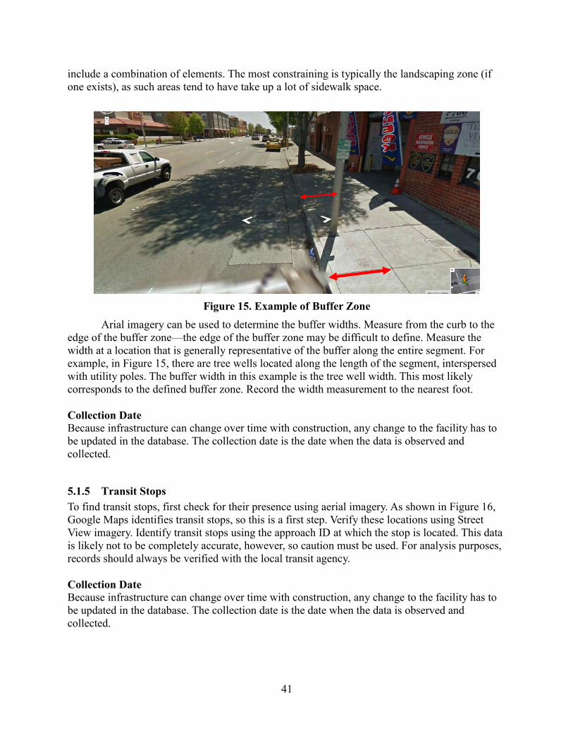
41

include a combination of elements. The most constraining is typically the landscaping zone (if one exists), as such areas tend to have take up a lot of sidewalk space.

Figure 15. Example of Buffer Zone

Arial imagery can be used to determine the buffer widths. Measure from the curb to the edge of the buffer zone—the edge of the buffer zone may be difficult to define. Measure the width at a location that is generally representative of the buffer along the entire segment. For example, in Figure 15, there are tree wells located along the length of the segment, interspersed with utility poles. The buffer width in this example is the tree well width. This most likely corresponds to the defined buffer zone. Record the width measurement to the nearest foot. Collection Date Because infrastructure can change over time with construction, any change to the facility has to be updated in the database. The collection date is the date when the data is observed and collected.

5.1.5 Transit Stops To find transit stops, first check for their presence using aerial imagery. As shown in Figure 16, Google Maps identifies transit stops, so this is a first step. Verify these locations using Street View imagery. Identify transit stops using the approach ID at which the stop is located. This data is likely not to be completely accurate, however, so caution must be used. For analysis purposes, records should always be verified with the local transit agency. Collection Date Because infrastructure can change over time with construction, any change to the facility has to be updated in the database. The collection date is the date when the data is observed and collected.

42

Figure 16. Transit Stops Shown in Google Maps

5.1.6 Bikeways Bikeway data is collected based on aerial imagery. Bikeways include any facilities for bicycles, ranging from shared-use lane marking (“sharrows”) to grade separated bicycle-only facilities. The most likely options to be encountered on the state highway network are bicycle lanes and sharrows. Bikeway Width Measure the width of the bikeway using aerial imagery (topdown, not 45 degrees, using distance measurement tool). If the facility is a marked shared use lane, measure the entire width of the lane. Bikeway Type Select the appropriate type of bikeway from the dropdown menu. The options include: Sharrows: As shown in Figure 17, these are painted symbols in a shared use lane to alert users that the facility is shared.

A_ID=3

Tran_ID=7

43

Figure 17. Example of “Sharrows”

(Source: http://streetswiki.wikispaces.com/Sharrow)

Bike Lanes: Separated facility for bicycles denoted by a single solid stripe of paint in between the lanes. See Figure 18.

Figure 18. Example of “Bike Lanes” (Source: http://streetswiki.wikispaces.com/Bike+Lanes)

44

Buffered Bike Lanes: Similar to a bike lane, but with a painted buffer zone in between the motor vehicle lane and the bicycle lane. See Figure 19.

Figure 19. Example of “Buffered Bike Lanes”

(Source: http://nacto.org/cities-for-cycling/design-guide/bike-lanes/buffered-bike-lanes/)

Bike Paths: Bike paths are separated facilities Bikeway Color Many jurisdictions are currently experimenting with different facility colors for bikeways. This practice has not been adopted by either the federal or California MUTCD, so it is unlikely to be encountered on state highways. However, this field is included in case the standards change. If the bikeway is painted (i.e., filled in), mark this as “painted,” otherwise mark it as “unpainted.” Collection Date Because infrastructure can change over time with construction, any change to the facility has to be updated in the database. The collection date is the date when the data is observed and collected.

5.1.7 Bike Parking Presence Bike parking facilities include bike racks and bike stations. The presence of any of these types of facilities along an approach should be recorded. Collection Date Because infrastructure can change over time with construction, any change to the facility has to be updated in the database. The collection date is the date when the data is observed and collected.

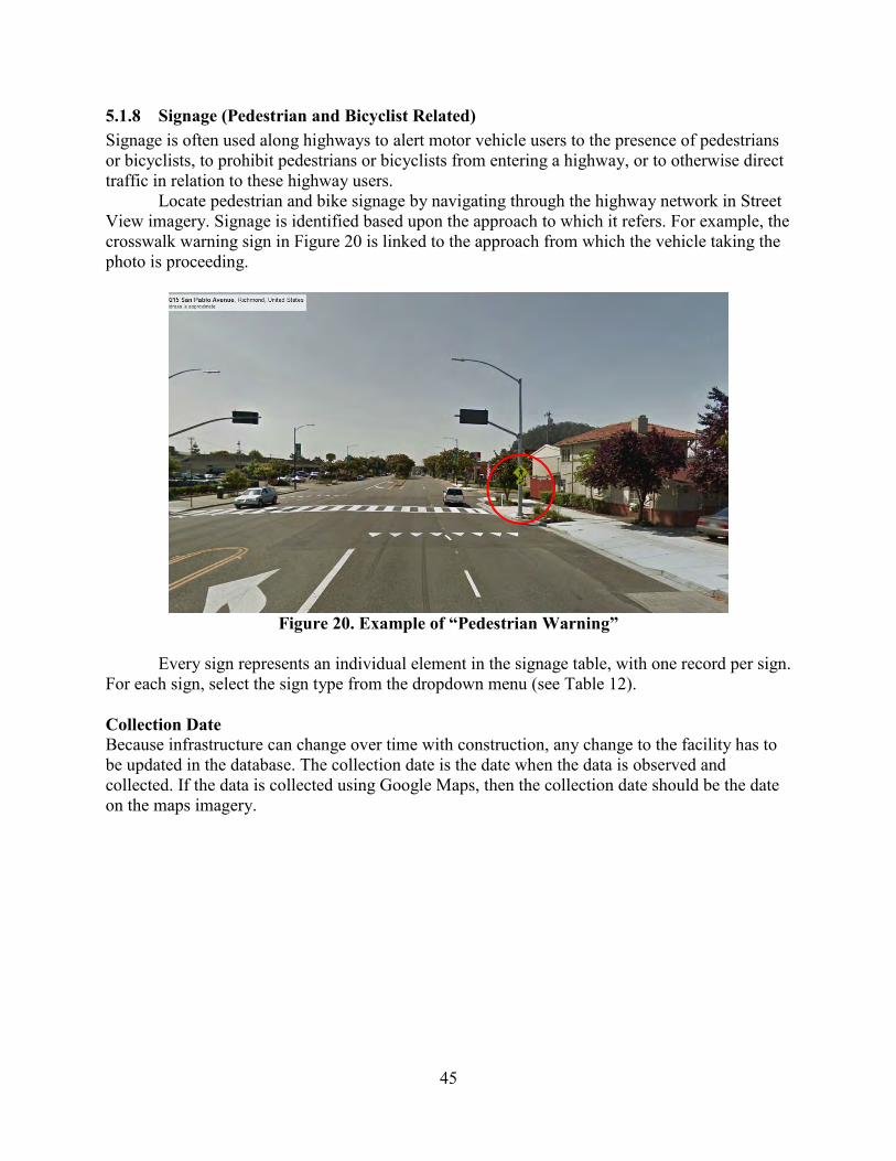
45

5.1.8 Signage (Pedestrian and Bicyclist Related) Signage is often used along highways to alert motor vehicle users to the presence of pedestrians or bicyclists, to prohibit pedestrians or bicyclists from entering a highway, or to otherwise direct traffic in relation to these highway users.

Locate pedestrian and bike signage by navigating through the highway network in Street View imagery. Signage is identified based upon the approach to which it refers. For example, the crosswalk warning sign in Figure 20 is linked to the approach from which the vehicle taking the photo is proceeding.

Figure 20. Example of “Pedestrian Warning”

Every sign represents an individual element in the signage table, with one record per sign.

For each sign, select the sign type from the dropdown menu (see Table 12). Collection Date Because infrastructure can change over time with construction, any change to the facility has to be updated in the database. The collection date is the date when the data is observed and collected. If the data is collected using Google Maps, then the collection date should be the date on the maps imagery.

46

Table 12. Pedestrian and Bicycle Related Signage Description Sign CA-MUTCD Sign

Designation

Pedestrian

W11-2

Bicycle

W11-1

No Pedestrian Crossing, Use Crosswalk

R49(CA)

No Pedestrian Crossing (symbol)/Use Crosswalk

R9-3, R9-3bP

No Bicycles

R5-6

Yield Here to Pedestrians/Peds

R1-5a/ R1-5

In-Street Ped Crossing

R1-6/R1-6a

Pedestrians, Bicycles, Motor-Driven Cycles Prohibited/Pedestrians and Bicycles Prohibited/Pedestrians Prohibited

R5-10a,b, c

Share the Road (plaque)

W16-1P

Turning Vehicles Yield to Peds

R10-15

Bicycles May Use Full Lane

R4-11

Other Pedestrian Signage Other Bicycle Signage

5.1.9 Crosswalks The crosswalk table is comprised of information pertaining specifically to marked crosswalks,

47

which require multiple core components for unique identification. Crosswalks can generally be identified based on aerial imagery. Each crosswalk is identified using one node ID and two approach IDs. CW_ID{I_ID, A_ID, A_ID}

The meaning of these identifiers is slightly different for various crosswalk arrangements. The three most common are below. Standard Intersection In Figure 21, crosswalk #4 is identified by node #2 and approaches #1 and #2. Crosswalk #5 is identified by approaches #3 and #1.

Figure 21. Example of Crosswalk Labeling for “Standard Intersection”

Midblock Crossing For midblock crossings, approach IDs are not used, instead such crossings are uniquely identified by node ID.

48

Slip Lane Crossing Crosswalk #5, across the slip lane in Figure 22, is identified by node #2, approach #2, and approach #4. This is a slightly different nomenclature than that found in the “standard intersection” case. In the standard case the approaches are those that the crosswalk crosses, however in the case of slip lanes, the approaches are those that the crosswalk lies between.

Figure 22. Example of “Slip Lane Crossing”

Collection Date Because infrastructure can change over time with construction, any change to the facility has to be updated in the database. The collection date is the date when the data is observed and collected. Position The position variable describes the location of each crosswalk on an intersection (i.e., the crosswalk on the south leg of the intersection). Options for position include south, north, east, west, southwest, southeast, northwest, and northeast. This variable should be identical to the one used in the pedestrian crosswalk volume table (see Section 4). Crosswalk Type A variety of crosswalk types exist, with newer designs intended to increase the visibility of the crossing. For every crosswalk, select the type used from the dropdown menu. The crosswalk types included in the data collection are: “unmarked,” “solid, standard,” “continental,” “dashed,” “zebra," and “ladder.” The possible types are also defined as in Figure 23:

49

Figure 23. Definition of Different Types of Crosswalks

(Source:http://www.dot.ca.gov/hq/esc/oe/project_plans/highway_plans/stdplans_US-customary-units_10/viewable_pdf/rspa24f.pdf)

50

Curb Ramp Curb ramps are the slopes used at intersections to increase accessibility. These facilities are highly important for people with disabilities, especially those in wheelchairs or those who are otherwise mobility impaired. For each crosswalk leg, note whether curb ramps exist on both sides of the crossing. The options for this field are as follows:

Two-Ramp (see Figure 24) One-Ramp (see Figure 25) Other—any other curb ramp design Combination—when one side of the crosswalk is a two-ramp curb ramp design and the

other is one-ramp None

Figure 24. Example of “Two-Ramp”

(Source: http://www.dot.ca.gov/hq/esc/oe/project_plans/highway_plans/stdplans_US-customary-units_10/viewable_pdf/rspa88a.pdf)

51

Figure 25. Example of “One-Ramp”

(Source: http://www.dot.ca.gov/hq/esc/oe/project_plans/highway_plans/stdplans_US-customary-units_10/viewable_pdf/rspa88a.pdf)

Detectable Warning Surfaces Detectable warning surfaces are a tactile and visual warning device used on curb ramps, at the edge of train platforms, and elsewhere to alert individuals with vision impairments to the presence of hazards. Curb cuts solve problems for people with mobility impairments, but may create a new hazard for those with vision impairments—namely, they eliminate the clear delineation between pedestrian right-of-way and automobile right-of-way. To address this issue, the standard is for these two treatments to be used in conjunction with each other.

In most cases, the surfaces are yellow, but they are available in a range of colors. This should generally be visible in the aerial imagery. For detectable warning surfaces, indicate the color ("yellow," "other," or "none"). Select the “none” option for locations where detectable surfaces are not present on both sides of the crosswalk. In the case of pedestrian refuge islands, similarly mark this field as “none” if detectable surfaces are not present at both ends of the crosswalk, as well as on both sides of the refuge island. Crossing Distance Crossing distance is measured between the two ends of the crosswalk. Because the curb is typically curved at intersections, measure along the side of the crosswalk away from the intersection, as shown in Figure 26, to ensure more consistent measurements between locations. Measurements can be made using aerial imagery, using the 45-degree mode. Similar to measuring the sidewalk widths, use the “Distance Measurement Tool.” First, click on the curb

52

where one end of the outside crosswalk line would intersect it, even if the paint doesn’t extend fully to the curb. Be careful to measure from the curb, not from the edge of the gutter pan (concrete section at edge of street abutting the curb). Click on the corresponding point on the opposite end of the crosswalk to determine the crossing distance.

Figure 26. Example of How to Measure Crossing Distance

In cases where there is a pedestrian refuge island(area in middle of crossing where pedestrians can stand and wait), measure the crossing distance including the median. There is a separate field for refuge island width.

For slip lane crossings, measure the leg of the crosswalk on the side facing oncoming traffic (i.e., the upstream edge). Crosswalk Color Crosswalk colors that are likely to be encountered are white and yellow (used in school zones), although others may also be observed. Select the paint color used for each crosswalk. Pedestrian Signal Head Presence/Pedestrian Signal Call Button Presence Pedestrian signal heads are attached to traffic signals to alert pedestrians to the pedestrian phase of the signal cycle. Pedestrian signal call buttons allow pedestrians to request a crossing phase. Both of these elements are associated with crosswalks. Similar to curb ramps and detectable warning surfaces, the presence of pedestrian signal head or signal call button should only be entered if observed on both sides of an intersection. These elements can only be observed in Street View imagery (see example in Figure 27).

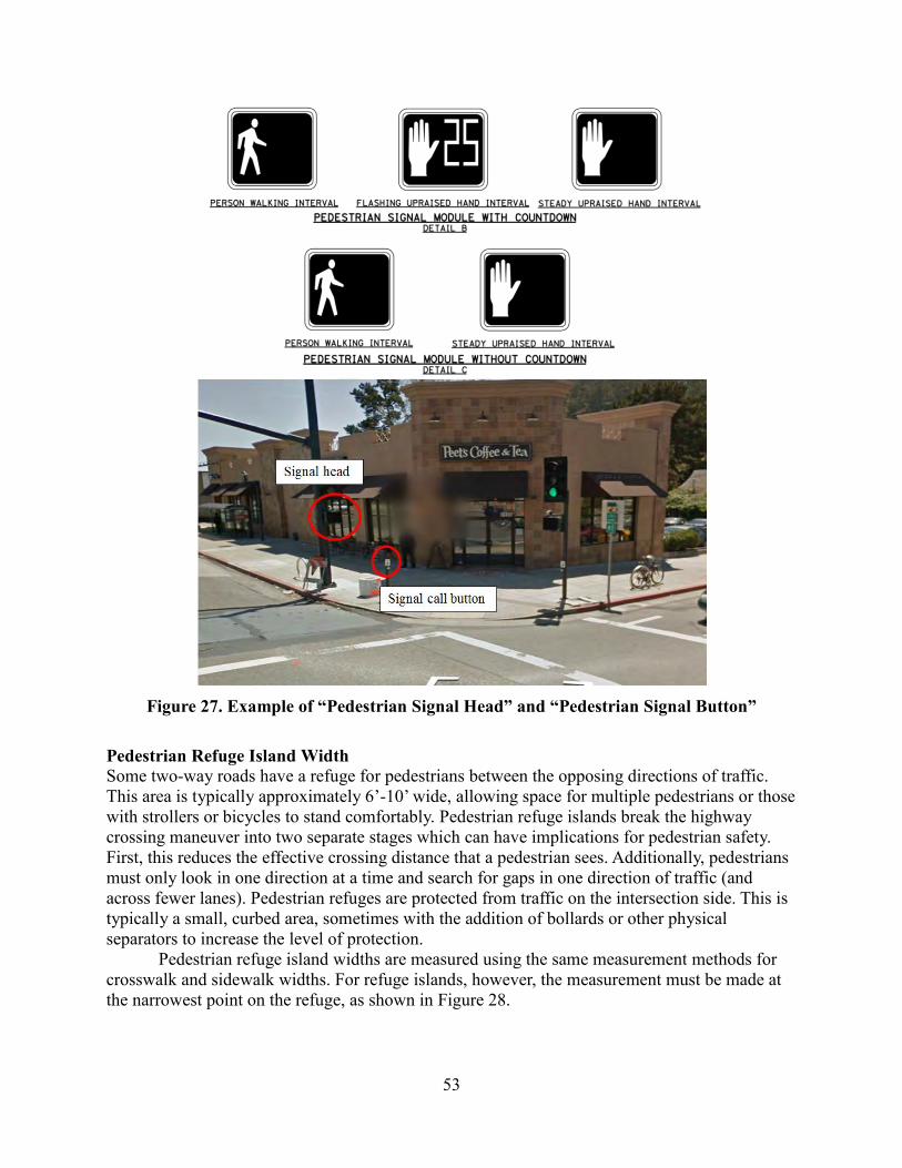
53

Figure 27. Example of “Pedestrian Signal Head” and “Pedestrian Signal Button”

Pedestrian Refuge Island Width Some two-way roads have a refuge for pedestrians between the opposing directions of traffic. This area is typically approximately 6’-10’ wide, allowing space for multiple pedestrians or those with strollers or bicycles to stand comfortably. Pedestrian refuge islands break the highway crossing maneuver into two separate stages which can have implications for pedestrian safety. First, this reduces the effective crossing distance that a pedestrian sees. Additionally, pedestrians must only look in one direction at a time and search for gaps in one direction of traffic (and across fewer lanes). Pedestrian refuges are protected from traffic on the intersection side. This is typically a small, curbed area, sometimes with the addition of bollards or other physical separators to increase the level of protection.

Pedestrian refuge island widths are measured using the same measurement methods for crosswalk and sidewalk widths. For refuge islands, however, the measurement must be made at the narrowest point on the refuge, as shown in Figure 28.

54

Figure 28. Example of How to Measure PedestrianRefuge Island Width

Advanced Stop Bar/Yield Warning Presence Advanced stop bars (Figure 29) and advanced yield warnings (Figure 30) are present at some crosswalks as mechanisms to increase pedestrian safety. Advanced stop bars are lines painted away from the crosswalk indicating where motor vehicles should stop. Advanced yield warnings (or “shark teeth”) are triangular markings located upstream of a crosswalk to notify drivers of the crosswalk and to inform them that they may have to yield.

Figure 29. Example of “Advanced Stop Bars”

(Source: saferoutesinfo.org)

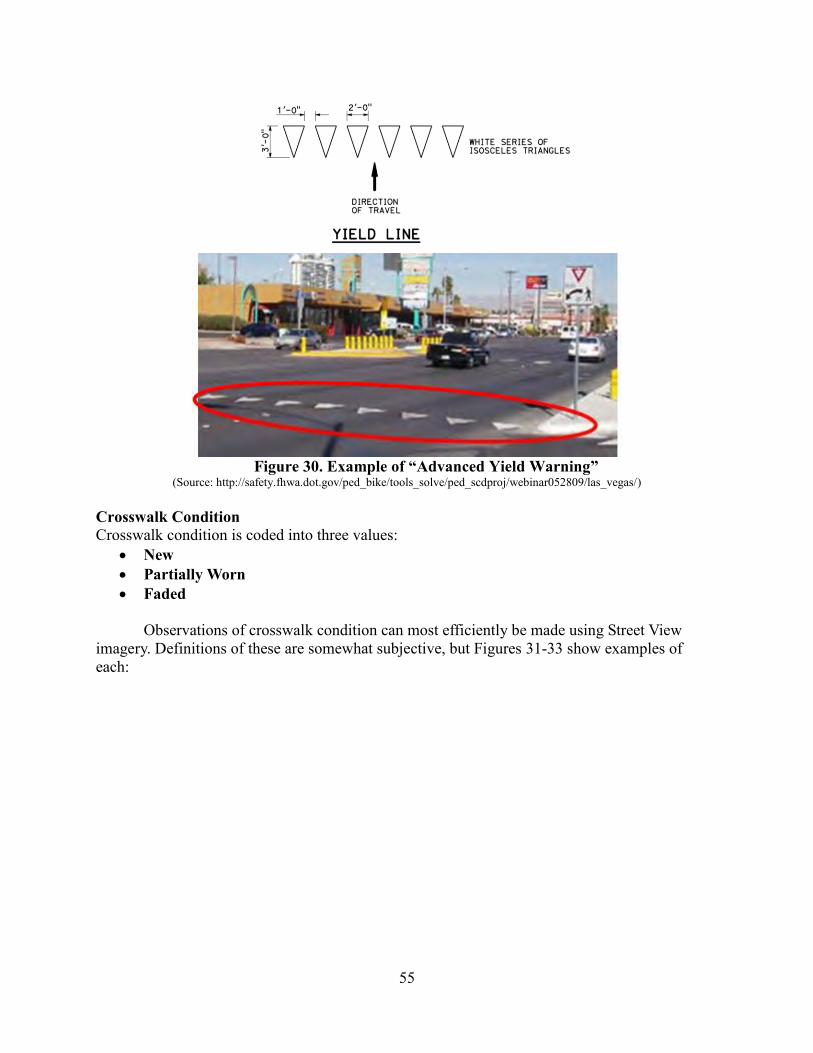
55

Figure 30. Example of “Advanced Yield Warning”

(Source: http://safety.fhwa.dot.gov/ped_bike/tools_solve/ped_scdproj/webinar052809/las_vegas/) Crosswalk Condition Crosswalk condition is coded into three values:

New Partially Worn Faded

Observations of crosswalk condition can most efficiently be made using Street View

imagery. Definitions of these are somewhat subjective, but Figures 31-33 show examples of each:

56

Figure 31. Example of “New” Crosswalk Condition

Figure 32. Example of “Partially Worn” Crosswalk Condition

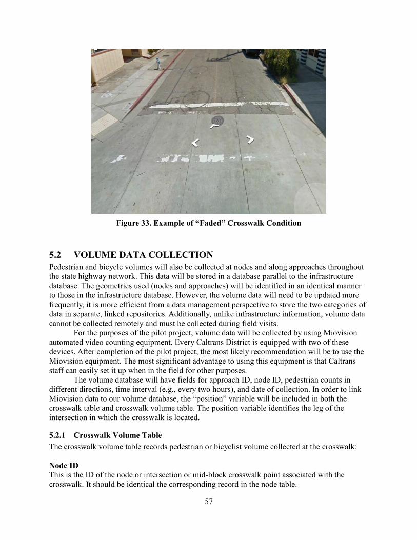
57

Figure 33. Example of “Faded” Crosswalk Condition

5.2 VOLUME DATA COLLECTION Pedestrian and bicycle volumes will also be collected at nodes and along approaches throughout the state highway network. This data will be stored in a database parallel to the infrastructure database. The geometries used (nodes and approaches) will be identified in an identical manner to those in the infrastructure database. However, the volume data will need to be updated more frequently, it is more efficient from a data management perspective to store the two categories of data in separate, linked repositories. Additionally, unlike infrastructure information, volume data cannot be collected remotely and must be collected during field visits.

For the purposes of the pilot project, volume data will be collected by using Miovision automated video counting equipment. Every Caltrans District is equipped with two of these devices. After completion of the pilot project, the most likely recommendation will be to use the Miovision equipment. The most significant advantage to using this equipment is that Caltrans staff can easily set it up when in the field for other purposes.

The volume database will have fields for approach ID, node ID, pedestrian counts in different directions, time interval (e.g., every two hours), and date of collection. In order to link Miovision data to our volume database, the “position” variable will be included in both the crosswalk table and crosswalk volume table. The position variable identifies the leg of the intersection in which the crosswalk is located.

5.2.1 Crosswalk Volume Table The crosswalk volume table records pedestrian or bicyclist volume collected at the crosswalk: Node ID This is the ID of the node or intersection or mid-block crosswalk point associated with the crosswalk. It should be identical the corresponding record in the node table.

58

Node Name This is the name of the street that intersects the main line. This value should be in the same format as it is in TASAS database so that is can eventually be linked to the TASAS database. Site Code This is the location information obtained from the Miovision data report. Position The position of the crosswalk indicates the leg of the intersection on which the crosswalk is located. The options include: “south,” “north,” “west,” “east,” “southwest,” “southeast,” “northwest,” and “northeast.” However, if the crosswalk is a mid-block crosswalk then the position information should be left blank. Direction1, Direction1 Volume, Direction2 Volume, and Bidirectional Volume Pedestrian volumes are defined directionally, based on the origin and destination ends of the crosswalk. If the volume count allows volume data to be collected for different directions, then these two fields should be completed. The corresponding volume value should be entered for “Direction1_vol” and “Direction2_vol.” If the volume count does not distinguish between directions, then the “Direction1_vol” and “Direction2_vol” should be left blank and the total volume of the two directions should be entered in the “Bidirectional volume” column. Interval The interval is the time period for collecting volume data. For example, if the pedestrian volume is tallied every 15 minutes, then the interval should be 15. Date This is recording date on which the volume is recorded. Start Time and End Time These values correspond to the time when the counter starts and finishes recording each volume value. Weather This information reflects the weather condition at the time of the volume data recording.

5.2.2 Approach (Sidewalk) Volume Table The approach volume table records pedestrian or bicyclist volume collected on the sidewalk along a specific approach:

Approach ID This is the ID of the approach associated with the sidewalk where the volume is recorded. It should be identical to the corresponding record in the approach table. Approach Name This is the name of the state highway on which the data is collected.

59

Site Code This is the location information obtained from the Miovision data report. Direction1, Direction1 Volume, Direction2 Volume, and Bidirectional Volume Pedestrian volumes are defined directionally, either parallel or anti-parallel to the direction of motor vehicle traffic on the corresponding approach. If the volume count allows volume data to be collected for different directions, then these two fields should be completed. The corresponding volume value should be entered for “Direction1_vol” and “Direction2_vol.” If the volume count does not distinguish between directions, then the “Direction1_vol” and “Direction2_vol” should be left blank and the total volume of the two directions should be entered in the “Bidirectional volume” column. Interval The interval is the time period for collecting each volume data. For example, if the pedestrian volume is tallied every 15 minutes, then the interval should be 15. Date This is recording the date on which the volume is recorded. Start Time and End Time These values correspond to the time when the counter starts and finishes recording each piece of volume value. Weather This information reflects the weather condition at the time of the volume data recording.

60

6 DATA COLLECTION PILOT To compare the time cost for potential data collection methods, we conducted a pilot for data collection both online and in the field. The pilot involved collecting data along approximately 100 miles (97.42 exactly) of the State Highway System, covering about 50 miles each in Districts 4 and 11 (see Table 13). In addition, a 7.3-mile field data collection effort was completed for comparison. This chapter details the pilot data collection process, including characteristics of the selected highways, and the procedure that data collectors followed.

Table 13. Routes for Computer Data Collection and Field Data Collection Data Collection

Method Route Name Mileage Roadway Classification District

Computer data collection

1 (SF 6.87 to 0.00) 5.2

urban multilane divided non-freeway

4

101 (SF T4.538R to SF 8.284R) 3.7 4

123 (ALA 0.228 to CC2.19) 7.51 4

75 (SD R 20.42 to SD 9.03) 11.04 11

82 (SCL 0.000 to SCL 15.353) 15.55 11

130 (SCL 0.000 to SCL 4.591) 3.84 11

13 (ALA9.87 to ALA 13.72) 5 urban 2 lane highway, urban

multilane divided non-freeway 4

5 (SD R32.826 to SD R 26.004 to SD

R16.123) 16.68 urban freeway 11

12 (SON 33.434 to SON 39.406) 6.1

mixture of urban multilane divided non-freeway, and urban 2 lane

highway 4

78 (SD N 17.72 to SD 40) 18.7

mixture of urban multilane divided non-freeway, rural multilane

divided non-freeway, and rural 2 lane highway

11

131 (MRN 0.000 to MRN 4.392) 4.1 rural multilane divided non-

freeway, and rural 2 lane highway 4

Field data collection

13 (from College Ave. to Ashby Ave.) 1.9 urban 2 lane highway, urban

multilane divided non-freeway 4

123(heinz to Stanford, Cutting

blvd to Moeser Ln) 2.1 urban multilane divided non-

freeway 4

12 2.5 mixture of urban multilane divided

non-freeway, and urban 2 lane highway

4

75 0.8 urban multilane divided non-freeway 11

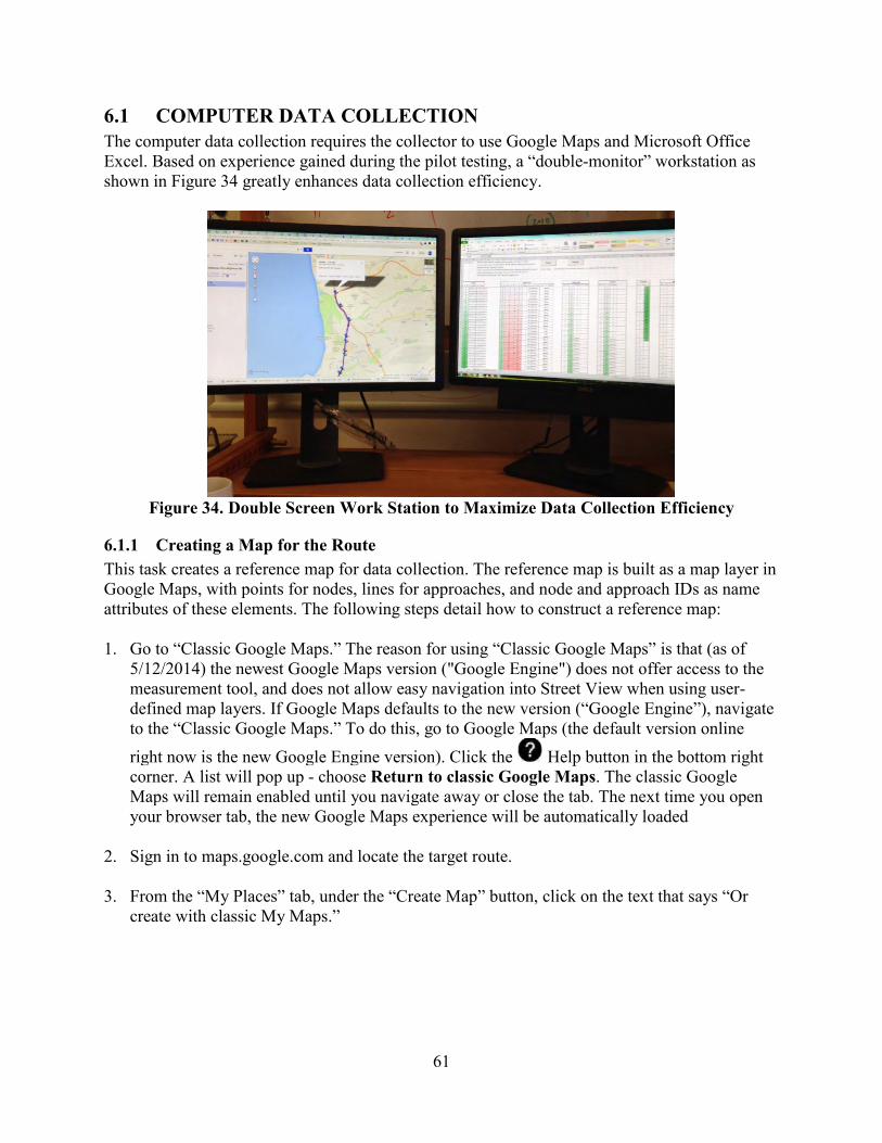
61

6.1 COMPUTER DATA COLLECTION The computer data collection requires the collector to use Google Maps and Microsoft Office Excel. Based on experience gained during the pilot testing, a “double-monitor” workstation as shown in Figure 34 greatly enhances data collection efficiency.

Figure 34. Double Screen Work Station to Maximize Data Collection Efficiency

6.1.1 Creating a Map for the Route This task creates a reference map for data collection. The reference map is built as a map layer in Google Maps, with points for nodes, lines for approaches, and node and approach IDs as name attributes of these elements. The following steps detail how to construct a reference map: 1. Go to “Classic Google Maps.” The reason for using “Classic Google Maps” is that (as of

5/12/2014) the newest Google Maps version ("Google Engine") does not offer access to the measurement tool, and does not allow easy navigation into Street View when using user-defined map layers. If Google Maps defaults to the new version (“Google Engine”), navigate to the “Classic Google Maps.” To do this, go to Google Maps (the default version online right now is the new Google Engine version). Click the Help button in the bottom right corner. A list will pop up - choose Return to classic Google Maps. The classic Google Maps will remain enabled until you navigate away or close the tab. The next time you open your browser tab, the new Google Maps experience will be automatically loaded

2. Sign in to maps.google.com and locate the target route.

3. From the “My Places” tab, under the “Create Map” button, click on the text that says “Or

create with classic My Maps.”

62

Figure 35. Illustration for Step 3

4. Reference the “Data collection manual,” shown in chapter 5, (henceforth referred to as “the

manual”), and familiarize yourself with the definitions of “node” and “approach.”

5. Start a stopwatch. You will record the time cost for labeling every 20 nodes/approaches, and record the time taken in the description box of the node and approach where you stop the watch. Then reset the stopwatch and repeat this process for another 20 nodes and approaches.

6. Name the map then click “done.”

Figure 36. Illustration for Step 6

63

7. Find the starting point. Search the starting point on the route (for example, the intersection of highway 123 and Solano Ave in Albany, California).

Figure 37. Illustration for Step 7

8. Save the starting point. Click “my places” and open the map you just created. For example,

map “route 123.” Left click the red bubble, a window will pop up, left click “save to map.”

9. Label the starting node. The bubble will be added to the map and turn blue. You will rename it using the ID index. Left click on the blue bubble and a window will pop up. You can then edit the title using node ID, for example: 1230001. Node labels should be in the format: xxxyyyy, where xxx is the highway route number with filler 0s on the left, and yyyy is the node number, with filler 0s on the left (i.e., 0130025 is node 25 on Highway 13. Close the window and the node point will be listed in the map information panel on the left side.

10. Label all the other nodes. Switch to satellite map background and zoom in. The map will

show you the default 45-degree view. Check along the route from the starting point (the first node you have been defined). Add the other nodes on the route. To do this, left click the “add point” tool icon. The mouse will change into a small cross on the screen. Go to the point where you want to add a node and left click the mouse, and the new point will be added. Assign it a new ID, (e.g., 1230002) in the title box. Finish labeling all of the nodes for the route. Keep in mind that nodes are defined to include intersections/junctions, midblock crosswalks, pedestrian overpasses/underpasses, and points every 1-mile if nothing else triggers the definition of a node.

11. Add approaches and label them. Zoom out so that you can see the two nodes of the

approach. Then left click the “add line” icon. Zoom it and left click near the starting point and drag the line to the location near the ending point and double click. The line is then completed and added. Name the line using the approach ID, (e.g., 1230001), numbering the approaches so that the direction of traffic corresponds to increasing odd numbers on one side of the road, and decreasing even numbers on the other side (1 is across from 2, 3 is across from 4, 5 is across from 6, etc.).

64

6.1.2 Using the Data Collection Macro Tool The data measured from Google Maps should be input and stored in the Data Collection Macro Tool (henceforth referred to as “the Macro Tool”), which is developed in Microsoft Office Excel. The macro tool contains two main spreadsheets. Details can be found in the Excel file contained in the deliverable package. The spreadsheet called “data” is where collectors input the measurements. The other spreadsheet called “time cost” can automatically record the time cost for each single input in the data spreadsheet. 1. In the “Data” spreadsheet, hit “Start” (once you hit “start,” the button will say “Stop”).

Enter data and the macro will automatically record the time costs for each cell on a separate sheet. (The ID for the “Sidewalk,” “Buffer,” “Transit,” “Bikeway,” “Bike parking,” “signage,” and “crosswalk” has been assigned in advance. You must add manually if you have additional rows.) After the pilot project, the “Time” sheet will no longer be used. This has been included simply for the purpose of estimating the total cost for the state highway network. The “Data” spreadsheet is the only item Caltrans will need for collecting data from the entire State Highway System. Hit the “Break” button if you want to take a break and leave the file open. The button will then change to “Resume”—to resume, press “Resume,” and the macro will automatically start recording time again. Hit the “Stop” button if you want to close the file.

6.1.3 Data Collection Step 1 Finish Group 1—Node Table 1. Open the map and the spreadsheet. Enter Node ID, Node Names, and Node Type in Node

Table, using “Satellite View.” Complete all nodes.

Step 2 Finish Group 2—Approach Table, Sidewalk Table, Buffer Table, Transit Table, Bikeway Table and Bike Parking Table 1. Enter Approach ID, From Node ID, and To Node ID in Approach Table, using “Satellite

View.” “Flag” is not required for every approach. You only need to input the Flag when there is a completed, abnormal intersection where the approach is not easy to identify. Otherwise, leave the Flag in blank. Reference the section 5.3.2 in the manual.

2. After finishing all approaches, enable “Ruler Tool” in classic Google Maps (the “Ruler Tool”

is not available in the new version of Google Maps called “Google Engine”). Note: A current bug with Google Maps may prevent the ruler icon from appearing. If this happens, disable the tool in Google Labs, save your changes, enable the tool again, and save your changes. This should resolve the issue. Click “Maps Labs," and enable the “Distance Measurement Tool.” A ruler should now appear in the bottom left corner of the map.

65

3. Using “Satellite View,” traverse the route once, gathering parking lane width, sidewalk width, bikeway width, and buffer width (the orange variables in the group 2 tables) for each approach using the ruler tool. If a sidewalk or approach does not exist, you should still record the approach in the A_ID column, but under “Width,” select “None.” If a bikeway, transit, signage, or bike parking does not exist, nothing needs to be recorded. NOTE: When measuring distance, be sure “45-degree” mode is disabled to ensure consistent measurements.

4. Using a split-screen “Street View” and “Satellite View” (see below), drag the “Street view” icon on the map to activate street view.

Note: Google Chrome users have reported being unable to use the split-screen view. Firefox and Internet Explorer do not seem to have this issue.

In the “Street View” mode, click the arrow icon in small box of satellite view on the bottom left corner. Split-screen will be displayed as below.

Figure 38. Illustration for Step 4

5. Traverse the route once in the direction of traffic flow, gathering median barrier effectiveness

for all approaches; and transit, signage, and bike parking for the approaches along the traffic flow. Navigate by clicking in the “Street View” to avoid missing data.

The “Satellite View” must be on one of the 3 most zoomed in views in order to see the transit symbols that Google has already marked. Use those symbols to check. They do NOT consistently capture every transit stop—however, if there is a symbol, it is probably correct.

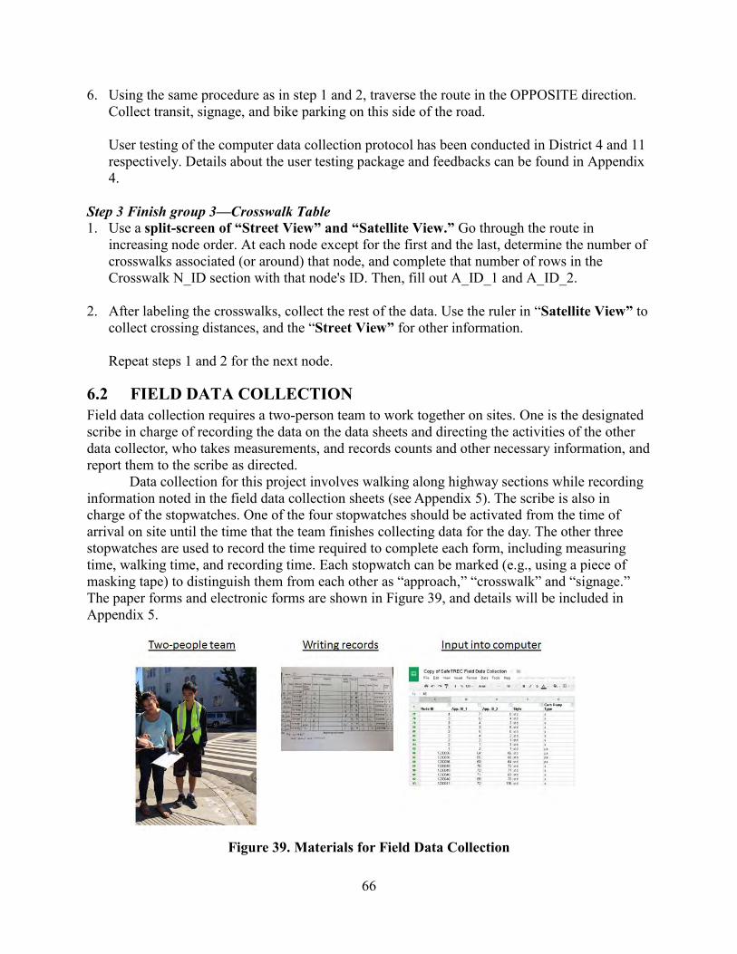
66

6. Using the same procedure as in step 1 and 2, traverse the route in the OPPOSITE direction. Collect transit, signage, and bike parking on this side of the road.

User testing of the computer data collection protocol has been conducted in District 4 and 11 respectively. Details about the user testing package and feedbacks can be found in Appendix 4.

Step 3 Finish group 3—Crosswalk Table 1. Use a split-screen of “Street View” and “Satellite View.” Go through the route in

increasing node order. At each node except for the first and the last, determine the number of crosswalks associated (or around) that node, and complete that number of rows in the Crosswalk N_ID section with that node's ID. Then, fill out A_ID_1 and A_ID_2.

2. After labeling the crosswalks, collect the rest of the data. Use the ruler in “Satellite View” to

collect crossing distances, and the “Street View” for other information. Repeat steps 1 and 2 for the next node.

6.2 FIELD DATA COLLECTION Field data collection requires a two-person team to work together on sites. One is the designated scribe in charge of recording the data on the data sheets and directing the activities of the other data collector, who takes measurements, and records counts and other necessary information, and report them to the scribe as directed.

Data collection for this project involves walking along highway sections while recording information noted in the field data collection sheets (see Appendix 5). The scribe is also in charge of the stopwatches. One of the four stopwatches should be activated from the time of arrival on site until the time that the team finishes collecting data for the day. The other three stopwatches are used to record the time required to complete each form, including measuring time, walking time, and recording time. Each stopwatch can be marked (e.g., using a piece of masking tape) to distinguish them from each other as “approach,” “crosswalk” and “signage.” The paper forms and electronic forms are shown in Figure 39, and details will be included in Appendix 5.

Figure 39. Materials for Field Data Collection

67

6.3 VOLUME DATA COLLECTION To complement the pedestrian infrastructure database currently being developed and integrated into the Caltrans TASAS database, ultimately a pedestrian and bicycle volume database will also be developed. This database will store pedestrian and bicycle volumes collected at intersections and along approaches throughout the state highway network. A likely approach for collecting this data is through the use of Miovision automated video counting equipment, which all Caltrans districts currently use for collecting motor vehicle volumes and turning movement counts. The current process for using the Miovision equipment is described below, in addition to the steps that should be taken to ensure that pedestrian and bicycle volume data is collected and formatted in a way that will enable fluid integration into the TASAS database.

6.3.1 Introduction to Miovision Data Miovision is a traffic data solution firm, which processes video data collected at intersections and roadway segments to produce data reports summarizing volumes and turning movement counts. Miovision customers also have access to an online portal where they can watch the videos, download data reports in various formats, view data collection locations on a map, and share data with other users. Traffic safety groups for the individual Caltrans districts each currently have two Miovision automated video counting devices, which are typically used to collect automobile traffic volumes and intersection turning movement counts. The traffic operations departments of some districts also have Miovision equipment, which are typically used to collect traffic volumes along freeways and at freeway ramps.

The typical process for collecting data is for the Caltrans district “user” to set up the portable Miovision equipment at an intersection or along a roadway segment. After a collection period, the user retrieves the equipment and uploads the video data to the specific Miovision online portal for that district. A username and password are required to access each portal, and information is not publicly available. When uploading the data, the user specifies the location of the study, the name of the study, and the classification type desired. Miovision then processes the data and provides data reports through the online portal. When collecting pedestrian and bicycle data, the process is similar to and should include the following considerations. The Miovision automated video counting equipment should be set up with a clear view of pedestrians and/or bicyclists using the study facility. When uploading the data to the Miovision portal, currently the user identifies the location of the facility on a map. However, the user also has the option of entering a “Site Code” for each recorded location. The user should enter the existing TASAS database intersection ID or mid-block location ID as the Site Code. This step is very important to ensure that the data can be appropriately linked to the TASAS database. Finally, when prompted for the “Classification Options,” the user should check the boxes which specify “Count Bicycles on Road,” “Count Pedestrians on Crosswalks,” and “Count Bicycles on Crosswalks,” as shown in Figure 40.

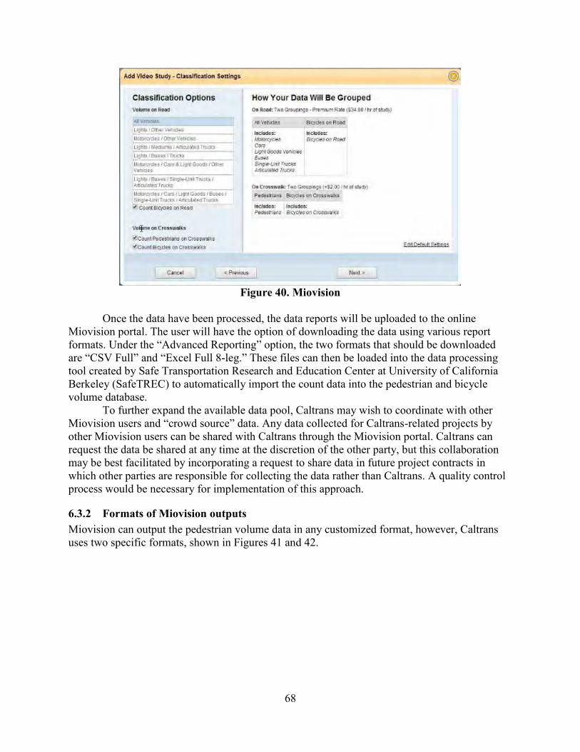
68

Figure 40. Miovision

Once the data have been processed, the data reports will be uploaded to the online

Miovision portal. The user will have the option of downloading the data using various report formats. Under the “Advanced Reporting” option, the two formats that should be downloaded are “CSV Full” and “Excel Full 8-leg.” These files can then be loaded into the data processing tool created by Safe Transportation Research and Education Center at University of California Berkeley (SafeTREC) to automatically import the count data into the pedestrian and bicycle volume database.

To further expand the available data pool, Caltrans may wish to coordinate with other Miovision users and “crowd source” data. Any data collected for Caltrans-related projects by other Miovision users can be shared with Caltrans through the Miovision portal. Caltrans can request the data be shared at any time at the discretion of the other party, but this collaboration may be best facilitated by incorporating a request to share data in future project contracts in which other parties are responsible for collecting the data rather than Caltrans. A quality control process would be necessary for implementation of this approach.

6.3.2 Formats of Miovision outputs Miovision can output the pedestrian volume data in any customized format, however, Caltrans uses two specific formats, shown in Figures 41 and 42.

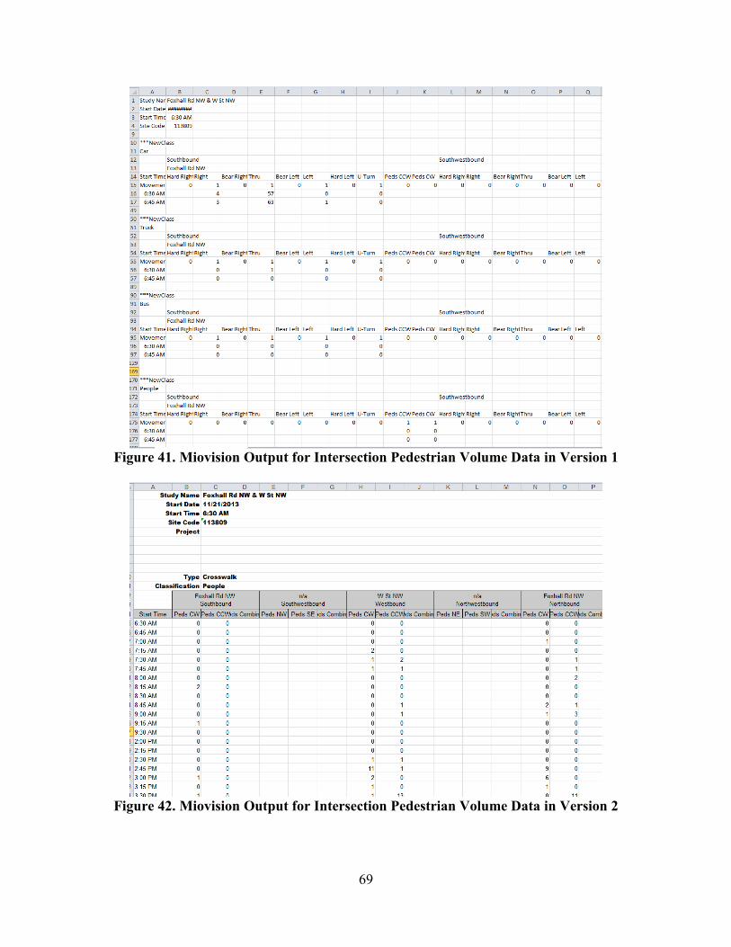
69

Figure 41. Miovision Output for Intersection Pedestrian Volume Data in Version 1

Figure 42. Miovision Output for Intersection Pedestrian Volume Data in Version 2

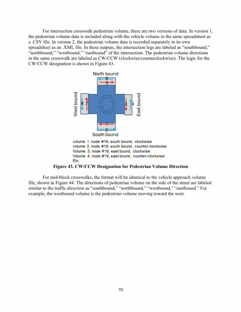
70

For intersection crosswalk pedestrian volume, there are two versions of data. In version 1, the pedestrian volume data is included along with the vehicle volume in the same spreadsheet as a .CSV file. In version 2, the pedestrian volume data is recorded separately in its own spreadsheet as an .XML file. In these outputs, the intersection legs are labeled as “southbound,” “northbound,” “westbound,” “eastbound” of the intersection. The pedestrian volume directions in the same crosswalk are labeled as CW/CCW (clockwise/counterclockwise). The logic for the CW/CCW designation is shown in Figure 43.

Figure 43. CW/CCW Designation for Pedestrian Volume Direction

For mid-block crosswalks, the format will be identical to the vehicle approach volume file, shown in Figure 44. The directions of pedestrian volume on the side of the street are labeled similar to the traffic direction as “southbound,” “northbound,” “westbound,” “eastbound.” For example, the westbound volume is the pedestrian volume moving toward the west.

71

Figure 44. Miovision Version 2 Output for Mid-Block Crosswalk Pedestrian Volume Data

6.3.3 Using the Data Importing Macro Tool To import the Miovision data into the proposed volume database, three macro tools have been developed. Two are for importing intersection pedestrian volume data from two versions of Miovision outputs, and the third is for importing approach pedestrian volumes from Miovision. Each of these macros will be used for a specific data format. For example, to import intersection pedestrian volume data in Miovision format version 1, the corresponding macro tool needs to be used. After the data is imported, it will be stored in the volume database as shown in Figures 45 and 46 separately for intersections and approaches.

Figure 45. Pedestrian Volume Database for Intersections

Figure 46. Pedestrian Volume Database for Approaches

72

7 TIME COST FOR DATA COLLECTION The time cost estimation presented in this chapter details the advantages and disadvantages of computerized and field data collection. While field data collection has traditionally been used and is familiar to many, widely available and free websites have introduced the option of data collection via computer. We considered the possibility of collecting pedestrian and bicycle facility data via Google Earth from a time cost perspective. I. Pilot Project on Time Estimation To determine the total estimated time cost for collecting pedestrian and bicyclist facility data across the California State Highway System, the progress of five research assistants collecting data on behalf of the pilot project was monitored. An Excel Macro sheet was used that recorded the time when students clicked ‘start,’ ‘break,’ or ‘end’ on the spreadsheet, as shown in Appendix 6. Each research assistant was assigned specific routes and instructed to collect pedestrian and bicyclist facility data via Google Maps. Each assistant was given verbal instructions, a manual that was still undergoing revisions, and an ‘expert’ contact person whom the assistant could consult regarding questions. We were interested in the rate at which data could be collected, which was expected to fluctuate depending on the roadway class, and the data collector’s speed of learning.

In summary, we can view the pilot project as an experiment to determine the capabilities of this data collection process. The pertinent variable to monitor is time, as the only significant input to this process is labor.

II. Estimation Procedure Upon the completion of data collection, we aggregated the time cost and determined the rate of data collection for each route. We classified each route according to one of ten categories. If a certain route changed categories within the route, for example from ‘Urban two way road’ to ‘Rural two lane road,’ two separate rates were calculated. The mileage for each rate was determined. We took the average rate of data collection per category, and used that to estimate the total time cost for statewide data collection. The entire process was conducted using programing software called “R.”

Table 14 below shows the route that we selected for our pilot project. For each route, we specify the nodes at which the data collector began and ended, the total mileage of the route, the total number of minutes recorded on the spreadsheet, and the data collector’s average pace in min/mile.

73

Table 14. Routes for Pilot Data Collection

Rte. Starting Node Ending Node Mileage Time cost (min)

Rate (min/ mile)

5 52 163 9.78 41 4.2

130 White Rd. Miguelito Rd. 1.64 234 142.7

82 280 Wolfe Rd. 8.95 367 41 123 MacDonald Ave. Solano Ave. 3.11 193 62 131 I-101 Main St. 4.1 165 40.2 75 4th Street & Glorietta Blvd. Highway 75 & Rainbow Dr. 9.14 334 36.5 75 Highway 75 & Rainbow Dr. Highway 75 & Highway 5 1.9 204 107.4

78 San Pasqual Valley & Bandy Canyon Road Julian Road & Paseo Pantera 10.2 115 11.3

12 Watmaugh Rd. Cavedale Rd. 6.1 250 40

1 Golden Gate Bridge 280-1 intersection (near Serramonte Mall) 5.2 192 36.9

13 I-80 I-24/freeway section 5 131 26.2 101 Marina Blvd. Central Fwy. 3.7 356 96.4 82 Blossom Hill Rd. 280 6.6 76 11.5 123 Solano Ave. I-580 4.4 203 46.1

5 56 52 6.9 8 1.15 130 101 White Rd. 2.2 383 174.2 78 Washington Ave & Ash St. Bandy Canyon Rd. 8.5 94 11.1

7.1 COMPUTER DATA COLLECTION In Table 15 below, we use the results from the pilot project to derive the total estimated time cost for collecting pedestrian and bicyclist facility data. The first column shows the roadway class, in which we categorized each route. The second column shows the total mileage per facility in the California State Highway System. The third column shows the mean rate of data collection per roadway class, and the fourth column shows the minimum and maximum observed rates from our pilot project. We obtained the total time estimation per row by multiplying the mean rate by the total existing mileage. Based on these estimates, the data collection is expected to take approximately 4,000 working hours to complete.

74

Table 15. Time Cost Estimation From Pilot

Roadway Class Mileage (mi)

Computer (min/mi) MEAN

Computer (min/mi)

MIN&MAX

Total Estimate

(hr) Urban freeways 3,533 2.67 1; 4.19 157.22 Urban freeways < 4 lanes 28 2.67a NA 1.25* Urban two lane roads 868 40.00 40.00; 40.00 578.67 Urban multilane divided non-freeways 1,081 49.00 11.50; 107.05 882.82 Urban multilane undivided non-freeways 176 29.17 21.44; 36.90 85.57 Rural freeways 2,879 2.10 2.10; 2.10 100.77 Rural freeways < 4 lanes 6 2.10b NA 0.21* Rural two lane roads 12,422 6.77 6.09; 7.46 1401.62 Rural multilane divided non-freeways 1,125 35.00 35.00; 35.00 656.25 Rural multilane undivided non-freeways 407 20.83c NA 141.30* Total 22,525 - - 4005.65

Notes: a This value is estimated by the urban freeways time cost assuming that urban freeways will have the same time cost no matter how many lanes there are. This is because there is rarely pedestrian facility on freeways so the time cost is only for navigating the map along the route. b This value is estimated by the rural freeways time cost with the same assumption as in note a

c this value is estimated by the rural multilane divided non-freeways. This is because we found that for urban multilane non freeways, the time cost for undivided are 60% of it is for divided. *The value is calculated based on specific assumptions.

7.2 FIELD DATA COLLECTION To compare the time cost of traditional field collection methods with computerized data collection, we also gathered field data on a subset of roadways. Table 16 below summarizes the rate of data collection on the field, as well as the total estimated working hours required to complete each category. We estimate that the time cost for traditional field data collection will be approximately 8,935 working hours.

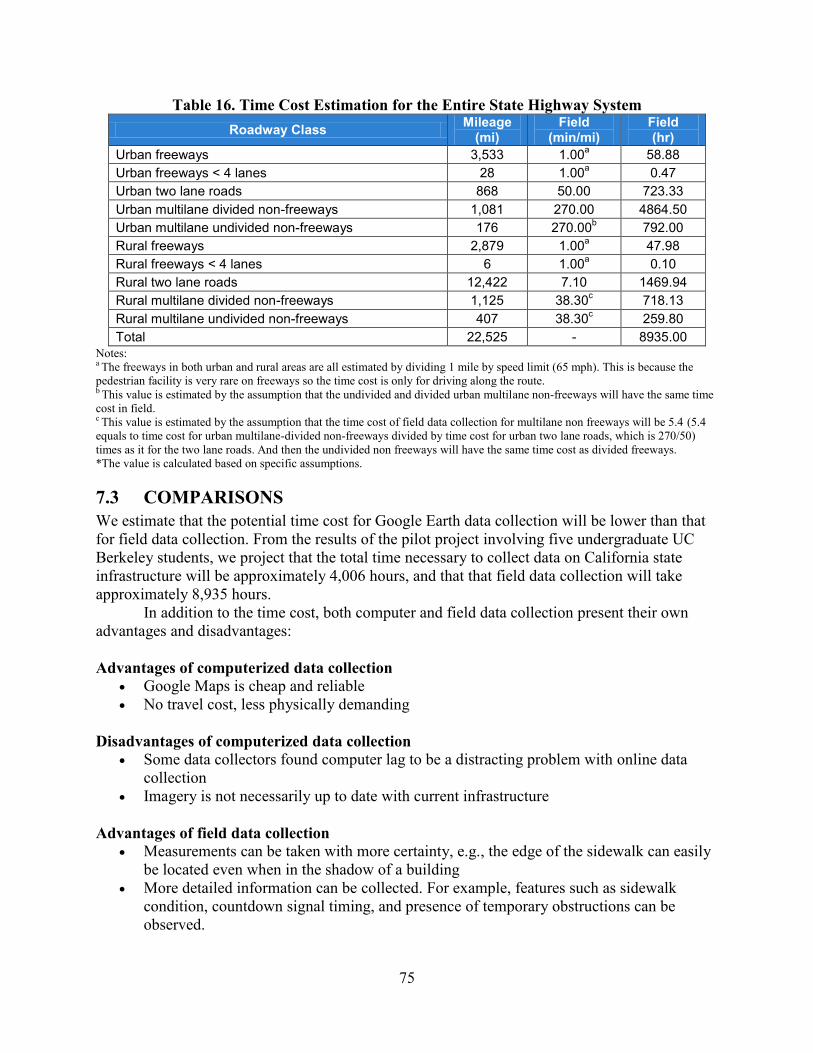
75

Table 16. Time Cost Estimation for the Entire State Highway System Roadway Class Mileage

(mi) Field

(min/mi) Field (hr)

Urban freeways 3,533 1.00a 58.88 Urban freeways < 4 lanes 28 1.00a 0.47 Urban two lane roads 868 50.00 723.33 Urban multilane divided non-freeways 1,081 270.00 4864.50 Urban multilane undivided non-freeways 176 270.00b 792.00 Rural freeways 2,879 1.00a 47.98 Rural freeways < 4 lanes 6 1.00a 0.10 Rural two lane roads 12,422 7.10 1469.94 Rural multilane divided non-freeways 1,125 38.30c 718.13 Rural multilane undivided non-freeways 407 38.30c 259.80 Total 22,525 - 8935.00

Notes: a The freeways in both urban and rural areas are all estimated by dividing 1 mile by speed limit (65 mph). This is because the pedestrian facility is very rare on freeways so the time cost is only for driving along the route. b This value is estimated by the assumption that the undivided and divided urban multilane non-freeways will have the same time cost in field. c This value is estimated by the assumption that the time cost of field data collection for multilane non freeways will be 5.4 (5.4 equals to time cost for urban multilane-divided non-freeways divided by time cost for urban two lane roads, which is 270/50) times as it for the two lane roads. And then the undivided non freeways will have the same time cost as divided freeways. *The value is calculated based on specific assumptions.

7.3 COMPARISONS We estimate that the potential time cost for Google Earth data collection will be lower than that for field data collection. From the results of the pilot project involving five undergraduate UC Berkeley students, we project that the total time necessary to collect data on California state infrastructure will be approximately 4,006 hours, and that that field data collection will take approximately 8,935 hours.

In addition to the time cost, both computer and field data collection present their own advantages and disadvantages: Advantages of computerized data collection

Google Maps is cheap and reliable No travel cost, less physically demanding

Disadvantages of computerized data collection

Some data collectors found computer lag to be a distracting problem with online data collection

Imagery is not necessarily up to date with current infrastructure Advantages of field data collection

Measurements can be taken with more certainty, e.g., the edge of the sidewalk can easily be located even when in the shadow of a building

More detailed information can be collected. For example, features such as sidewalk condition, countdown signal timing, and presence of temporary obstructions can be observed.

76

Disadvantages of field data collection Travel time is substantial, especially for sites that are not near the local Caltrans office Measuring in the field can be dangerous, especially along high-speed highways

Because the computer data were gathered by multiple collectors, personal variance

undoubtedly exists. The working environment, learning curve, and other day-to-day factors can cause time cost fluctuations even when the data are collected by a single individual. Accordingly, time-cost estimates have been presented as a range. Even when considering the upper end estimate, the time cost for computer collection totals approximately 4,786 working hours, which is substantially lower than the amount of time required for field data collection. Therefore, we can conclude that the computer time cost is no more than 50% of the time cost for field data collection.

In addition, the timer we developed in the Microsoft Excel Spreadsheet can also introduce bias. For example, if the data the collector forgets to press the start/stop button after taking a break in the timing, the recorded time cost will be less than the actual time expended. However, to calculate an estimate, we assume that various instances of bias will balance out.

77

8 CONCLUSIONS AND RECOMMENDATIONS

8.1 CONCLUSIONS This project aims to build a data collection plan for Caltrans to collect pedestrian infrastructure and volume data to supplement the TASAS database. The possibility of adding additional pedestrian related data such as infrastructure and volume into the TASAS database is discussed in Chapter 2. The decision was made to develop an “add-on” database, parallel to TASAS with key links to connect the two together. The measurements required by the database were decided both from the perspective of management and analysis. Pedestrian infrastructure and volume data will be stored in two separate databases with the same key fields to connect to each other and to the TASAS database. The definitions and measuring methods for all the components are described in detail in Chapter 5. The database and measuring methods have been tested in a pilot data collection effort. In the pilot, 100 miles of state highways were selected for computer-based data collection, of which approximately one tenth were also used for field data collection. The computer and field data collection procedures are developed and documented in the data collection manual and tutorial (Ch. 5 and 6) to guide data collection work in the future.

For this effort, the databases were developed in Microsoft Excel spreadsheet format to store the pedestrian infrastructure data and to automatically import volume data from files produced by Miovision. To estimate the time cost for the two data collection methods, the cost for each measurement was recorded in parallel with the database and is then compared for collecting data from the entire State Highway System. Results indicate that the computer time cost will be approximately 4,000 working hours, which is no more than 50% of the time cost estimated for field data collection. The following conclusions are based on the analyses conducted during the project: 1. The database developed in this project offers flexibility in its ability to connect to TASAS, is

easy to update and maintain, and allows new records and measurements to be added without any changes to TASAS. The procedure for data collection defined in this report will be useful for future implementation of the data collection plan. Caltrans will decide whether the pedestrian infrastructure and volume database is going to be merged into TSN or developed as a separate database with links to TSN.

2. The measurements suggested for inclusion in the database adequately cover pedestrian related facilities to help Caltrans track facility coverage. In addition, these measurements are useful for pedestrian safety analysis and can offer critical information for safety investigations and countermeasure selection.

3. The time estimates for collecting pedestrian infrastructure and volume data indicate that the computer data collection is more durable than the field data collection. Use of Google Maps is much less costly (more than 50% less) in terms of time than performing field data collection, even without considering site access time. Although field data collection offers the advantage of data collectors being able to see every corner of a street, the accuracy of the measurements based on computer data collection appears to be fairly high.

78

8.2 RECOMMENDATIONS Complete State Highway Network Inventory The primary recommendation of this project is for Caltrans to initiate construction of the proposed database within TSN and initiate the full infrastructure inventory. As has been discussed, computer-based data collection for the entire state highway network could be completed with approximately 4,000 staff-hours, or approximately 2.0 Full-Time Equivalent (FTE)-years. Additional certainty in data could be achieved by conducting field-based inventory for the urban portions of the state highway system. Alternatively to a full-fledged data collection effort, Caltrans staff could collect data during routine field visits to enter into the database once constructed, and thereby incrementally populate the database for minimal additional cost. In either case, the first next step would be for the database to be constructed by HQ to accommodate data collection. HQ will then need to provide the Districts with resources to complete the data collection. Allocation of resources should reflect the approximate expected data collection costs per district. Finally, a protocol should be developed for continual maintenance of the new database, likely mirroring that used for updates of the TASAS database. Linking to the Existing TASAS-TSN Database One of the most important improvements to be made to this database is to connect it to the existing TASAS database. The data collection process was designed with this connection in mind, so that existing fields do not have to be re-collected. The connection process will involve making connections between the intersections IDs in TASAS and the node IDs in the new database. One possible key link could be the combined information of intersection connection ID and begin date which are currently used in TSN and TASAS to uniquely identify each intersection. A protocol for merging this link into the infrastructure database is proposed below.

1. All of the intersections in the TSN or TASAS database will be mapped in GIS environment or Google Maps using the location information, including route name, suffix, direction, prefix, county, and post mileage. All of the intersection point data will maintain the information of intersection connection ID and begin date which can connect the list to the data in the TSN/TASAS

2. Data collectors will work directly on the map of TSN/TASAS intersections, and will confirm that the locations of the intersection points are correct and make corrections if necessary by dragging the points to the correct locations.

3. Data collectors will continue work on the confirmed intersection map to label the intersections using the node ID, and insert mid-block crosswalks and other types of nodes into the map. It should be noted that these added nodes do not have to be connected to TSN/TASAS, so long as the intersections are connected with a one-to-one relation.

4. Approaches will be labeled and other data collection processes will be conducted according to the data collection tutorial in Appendix 4.

GIS-Based Framework This database could potentially be implemented as a Geographic Information System (GIS), which would provide spatial references for all of the elements that are collected. Using GIS might make the data entry process more burdensome and difficult, as it requires a specialized set of skills. It would also potentially make connecting to the existing TASAS database more difficult, as TASAS is currently stored in an Oracle database, not geographically. However,

79

using a GIS framework could make analysis of the collected data more straightforward in the long run. Additionally, some information, such as lengths of sidewalks and crossing distances could be automatically calculated based on the geometries of the shapes that are drawn. Inclusion of Additional Variables After the completion of the pilot data collection process, a number of additional variables were suggested for inclusion in the database. These variables should be considered for the final database, as they will not add substantial cost to the data collection and can easily be accommodated by the proposed structure.

Pedestrian countdown signal: It should be noted whether pedestrian signal heads include countdown timers, as these are a proven effective pedestrian safety countermeasure. Data collection may require field visits, as street-level imagery does not consistently capture the signal at a point in time where the countdown numbers are visible. Alternatively, data could be recorded based on review of existing data sources.

Bicycle detection: Signalized intersections should be noted as having bicycle-actuated signals. This may not be collectible from field inventory, and may require review of existing documentation.

Freeway On-/Off-Ramps The current data collection procedure does not direct data collectors to include freeway on- and off-ramps in the database. In one sense, freeway underpasses with sidewalks crossing on-/off-ramps are an intersection between the motor vehicle network and the non-motorized network. On- and off-ramps are crucial locations to consider when addressing pedestrian and bicycle safety, as these locations tend to experience high crash rates. Accordingly, future iterations of this database should include the capability to include intersections between the underlying street network and high ramps. This should fit easily to the database format developed during the current project, however the data collection protocol will need to be modified accordingly. Local Jurisdiction Involvement Local jurisdictions could additionally be trained on the data collection protocol and collect similar data on their streets for comparable analysis. Caltrans could host this database to allow for comprehensive systemic analysis of the statewide road network, including both state highways and local roads.

80

Implementation of Tablet Computer Interface for Field Data Collection Field data collection currently relies on a series of three forms for recording measurements, which are later entered manually into the computer back in the office. This process could be dramatically improved by developing an interface for tablet computers to enter data taken in the field. This could be as simple as creating electronic forms with dropdown menus for entry types, or as elaborate as a Google Maps interface which would allow the user to select highway elements and then enter measurements into a pop-up dialog box, providing geolocation for the data. Additionally, if a tablet with GPS transmittance was used, real-time coordinates could be included with the data as it is collected to simplify the geolocation process. Hybrid/Computer-Focused Data Collection Process Based on the pilot data collection project, a hybrid approach between computer and field-based data collection is recommended. Computer data collection should be the core of the process, due to its much faster data collection times and minimal loss of detail/accuracy. However, when Caltrans staffs are in the field, measurements should be taken by hand to validate the computer data collected and to improve the quality of information in the database.

81

APPENDIX 1. NOTES FROM INTERVIEW WITH ERIC FREDERICKS, CALTRANS DISTRICT 3 August 2, 2012 On the Call: Eric Fredericks, Robert Schneider, Frank Proulx During call, Frank Proulx and Robert Schneider interviewed Eric Fredericks about the Caltrans District 3 Complete Streets Inventory Data Fields Included are Shown in Public Online Database (http://www.dot.ca.gov/dist3/departments/planning/communityplanning1.htm) Avoided some fields for public release due to legal issues, including:

Anything suggesting substandard facilities Any widths due to accuracy worries Any segments noted with “Planning to Review Further” serve as a flag that there might

be something substandard here. Noted that database is very fact-based, avoiding speculation as much as possible.

Data Collected by Volunteers

Just filling out DB for Sacramento Area Counties took roughly 3 months at 35-40 hours/week (very rough estimate)

Most data collected using Google Street View, some inconsistencies determined between Street View and aerial view, which were then checked against the Caltrans photo log

Data collected along Caltrans highways, plus intersecting local roadways where interactions with state highways exist

Skipped very rural roads where pedestrians/bicyclists were extremely unlikely to be found Caltrans District 3 plans to use this database primarily for prioritization of projects, as

well as for reference when applying for funding for improvements. Eric heavily emphasized that his priority was getting a product out quickly, not

deliberating over what fields should or should not be included. He simply picked those that would be very important for his purposes, and gave his first volunteer some discretion regarding including others. He stressed to us the importance of getting a large group of people onboard with our ideas for which fields to include quickly, so as to not waste too much time on this task.

Maintenance of the database has not been discussed, but he suggested that if anybody brings up an inconsistency between the data and the ground truth that it will be fixed immediately.

Noted that some roads (e.g. El Camino Real) will take far more time to document than others (freeways)

Database includes a field for probability of bike/ped presence, which was determined heuristically:

High – Many activity uses nearby plus high quality facilities Medium – Either many activity uses with moderate facilities, or High quality facilities

with lower levels of activity generating land uses Low – No activity generators and lower quality/non-existent infrastructure

82

Database includes links to Google Street View by clicking on location. Trying to get it implemented into an interactive map, but will involve changing the postmile designations to link to a map.

83

APPENDIX 2. NOTES FROM INTERVIEW WITH DAROLD HEIKENS, CALTRANS ADA INFRASTRUCTURE PROGRAM CHIEF October 8, 2012 On the Call: Darold Heikens, Robert Schneider, Frank Proulx Darold provided details of the construction of a statewide ADA non-compliant facility inventory, part of the federally mandated ADA transference plan

The inventory includes all non-compliant facilities along State Highways, defined as extending to the back edge of the sidewalk. Local cross streets abutting the Highways were not included, nor were on/off ramps, bridges, or underpasses.

Data was collected in two phases, by Northern and Southern California. Work was contracted out to a consulting firm. Facilities were inspected for compliance using tape measures and smart levels. During the first phase, data was recorded on paper and later entered in to a computer spreadsheet. During the second phase, a tablet computer was used, which allowed for in-the-field geo-referencing, and made data collection much easier.

Data is all referenced using the State Highway postmile system as well as geo-referencing codes

Data is currently stored on the consultant’s servers, but will eventually be moved over to Caltrans servers. Currently stored in a Google Earth format, but will be integrated into the CT Earth architecture. CT Earth is generally preferable to a database format due to its geo-referencing capabilities and superior user interface, as this inventory will be publicly available in some form.

Facilities are marked as non-compliant, as well as providing information on (1) what particular aspects of the facility are out of compliance, and (2) how far outside the acceptable range they are

Districts are currently asked to record any improvements that they make to the non-compliant facilities, which will later be updated at the HQ level. There is internal discussion as to how much control districts will eventually have over the inventory, and if they will be asked to update the database themselves or submit updates to a central controller.

Data is used for identification and prioritization of ADA non-compliant facilities Future goals include testing LIDAR to identify curb ramps and other pedestrian facilities,

as well as collect elevation data for the use of designers working to redesign facilities and bring them to compliance. This will reduce the need for surveyors to collect elevations, which currently must be done prior to any project where no elevation data has been recorded.

84

APPENDIX 3. NOTES FROM INTERVIEW WITH DEBRA KINGSLAND, NEW JERSEY DOT BIKE & PEDESTRIAN PROGRAM SECTION CHIEF July 11, 2012 On the Call: Debra Kingsland, Robert Schneider, Frank Proulx During call, Frank Proulx and Robert Schneider interviewed Debra about NJDOT’s County Roads Pedestrian Infrastructure Inventory. Data Fields Collected:

Sidewalk Presence Curb Ramp Presence Sidewalk Width Shoulder Width Sidewalk Condition (Good, Fair, or Poor) Sidewalk Material (Concrete, Asphalt, etc.) Pedestrian Signage Pedestrian Signals @ Intersections ADA Compliance

Data Collection Methodology: A van was driven along all county roads, equipped with digital cameras on front & side, and a GPS locator. Photos taken every ~2 seconds, saved with GPS coordinates. Photos then analyzed by hand and data recorded into database. Database made available to counties, including upload of data to portable HDDs and training on how to use data. A state highway system inventory was also conducted. Challenges faced:

Time of Year/Weather Snow on ground can’t collect ped infrastructure data Rainy days Cameras fogged up Darkness posed issue (esp. during Winter months)

Cost: Roughly $750k (USD 2007) for entire county road system, including data collection(van driving), data extraction, and training of counties on how to use the data Data was turned over to counties for use in pedestrian planning Discussion at state level of creating a Pedestrian Safety Management System Images used to look up conditions remotely Messages for Caltrans:

Make sure company knows how to conduct the video analysis, can extract features that are desired, has access to necessary equipment, and can put data into a useable format

Images are in an ESRI GeoDatabase, can be viewed at in ArcMap

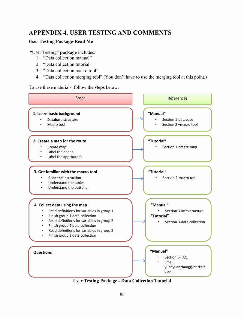
85

APPENDIX 4. USER TESTING AND COMMENTS User Testing Package-Read Me “User Testing” package includes:

1. “Data collection manual” 2. “Data collection tutorial” 3. “Data collection macro tool” 4. “Data collection merging tool” (You don’t have to use the merging tool at this point.)

To use these materials, follow the steps below. User testing memo

User Testing Package - Data Collection Tutorial

1. Learn basic background • Database structure • Macro tool

“Manual” • Section 1-database • Section 2 –macro tool

2. Create a map for the route • Create map • Label the nodes • Label the approaches

“Tutorial” • Section 1-create map

3. Get familiar with the macro tool • Read the instruction • Understand the tables • Understand the buttons

“Tutorial” • Section 2-macro tool

4. Collect data using the map • Read definitions for variables in group 1 • Finish group 1 data collection • Read definitions for variables in group 2 • Finish group 2 data collection • Read definitions for variables in group 3 • Finish group 3 data collection

“Manual” • Section 3-infrastructure

“Tutorial” • Section 3-data collection

Steps References

Questions “Manual” • Section 5-FAQ • Email:

yuanyuanzhang@berkeley.edu

86

Create a Map for the Route This task creates the map for the data collection, including adding points for nodes, adding lines for approaches, and assigning the node IDs and approach IDs for nodes and approaches. 1. Go to “Classic Google Maps.” The reason for using “Classic Google Maps” is that (as of

5/12/2014) the newest Google Maps version ("Google Engine") does not offer access to the measurement tool, and does not allow easy navigation into Street View when using user-defined map layers. If Google Maps defaults to the new version (“Google Engine”), navigate to the “Classic Google Maps.” To do this, go to Google Maps (the default version online right now is the new Google Engine version). Click the Help button in the bottom right corner. A list will pop up - choose Return to classic Google Maps. The classic Google Maps will remain enabled until you navigate away or close the tab. The next time you open your browser tab, the new Google Maps experience will be automatically loaded, or you can just click this link to go to old version. https://www.google.com/maps?t=m&ll=37.87077539999999%2C-122.30098000000004&spn=0.12372723260514347%2C0.20899178791223869&output=classic&dg=opt

2. Sign in to maps.google.com and locate the target route.

3. From the “My Places” tab, under the “Create Map” button, click on the text that says “Or

create with classic My Maps.”

4. Reference the “Data collection manual,” (henceforth referred to as “the manual”), and familiarize yourself with the definitions of “node” and “approach.”

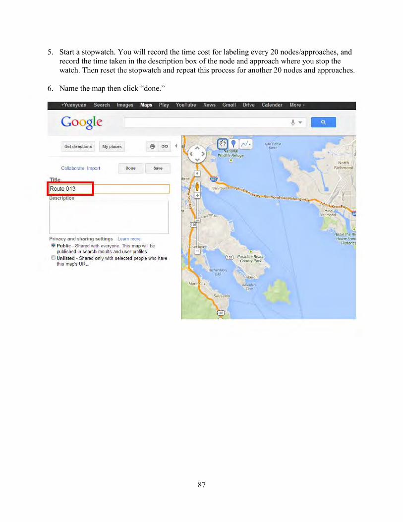
87

5. Start a stopwatch. You will record the time cost for labeling every 20 nodes/approaches, and record the time taken in the description box of the node and approach where you stop the watch. Then reset the stopwatch and repeat this process for another 20 nodes and approaches.

6. Name the map then click “done.”

+Yuanyuan Search Images Maps Play You Tube News Gmail Drive Calendar More·

Coogle

Get directions My places

Collaborate Import Done Save

liRoute 013 I

Privacy and sharing settings Learn more

@ Pub lic - Shared with everyone. This map will be published in search results and user profiles.

(5 Unlisted - Shared only with selected people who have this map's URL.

~ @) Paradise Beach

CounryPark

Richardson Bay

t§J

Tiburon

Belvedere ClNe

-North

Richmond

. ~ Ros1e theRn HomeFronl

Historicc

~ ----------------------~----------~

88

7. Find the starting point. Search the starting point on the route, for example, the intersection of highway 123 and Solano Ave in Albany, CA is the starting point.

8. Save the starting point. Click “my places” and open the map you just created. For example, map “route 123”. Left click the red bubble, then a window pops up and Left click “save to map”

9. Label the starting node. The bubble will be added to the map and turn blue. You will rename it using the ID index. Left click on the blue bubble and a window will pop up. You can then edit the title using node ID, for example: 1230001. Node labels should be in the format: xxxyyyy, where xxx is the highway route number with filler 0s on the left, and yyyy

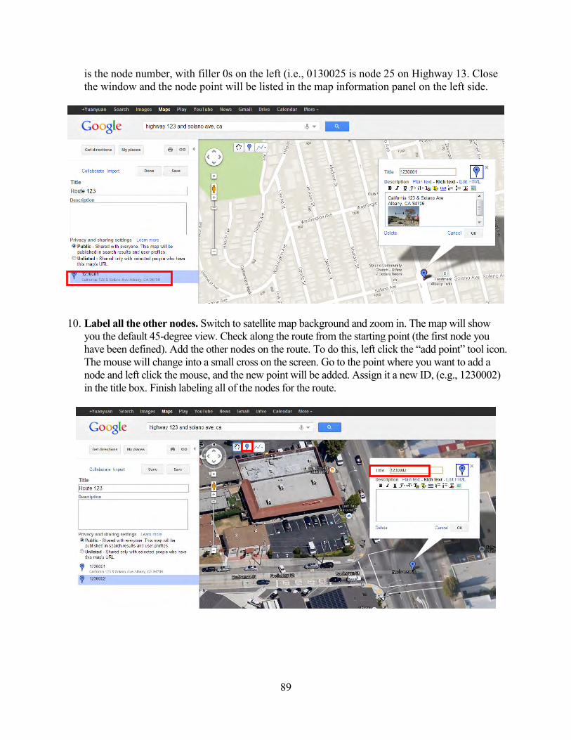
89

is the node number, with filler 0s on the left (i.e., 0130025 is node 25 on Highway 13. Close the window and the node point will be listed in the map information panel on the left side.

10. Label all the other nodes. Switch to satellite map background and zoom in. The map will show

you the default 45-degree view. Check along the route from the starting point (the first node you have been defined). Add the other nodes on the route. To do this, left click the “add point” tool icon. The mouse will change into a small cross on the screen. Go to the point where you want to add a node and left click the mouse, and the new point will be added. Assign it a new ID, (e.g., 1230002) in the title box. Finish labeling all of the nodes for the route.

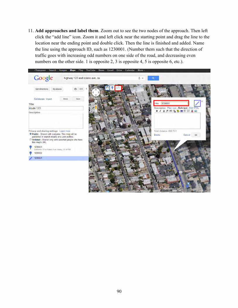
90

11. Add approaches and label them. Zoom out to see the two nodes of the approach. Then left click the “add line” icon. Zoom it and left click near the starting point and drag the line to the location near the ending point and double click. Then the line is finished and added. Name the line using the approach ID, such as 1230001. (Number them such that the direction of traffic goes with increasing odd numbers on one side of the road, and decreasing even numbers on the other side. 1 is opposite 2, 3 is opposite 4, 5 is opposite 6, etc.).

91

Using the Data Spreadsheet 1. Hit “Start” (once you hit “start”, the button will turn to “Stop.”)

That’s it! Enter data and the macro will automatically record the time costs for each cell on a separate sheet. (The ID for the “Sidewalk,” “Buffer,” “Transit,” “Bikeway,”,“Bike parking,” “signage,” and “crosswalk” has been assigned in advance. You must add manually if you have additional rows.)

Hit the “Break” button if you want to take a break and leave the file open. The button will then change to “Resume”—to resume, press “Resume,” and the macro will automatically start recording time again. Hit the “Stop” button if you want to close the file.

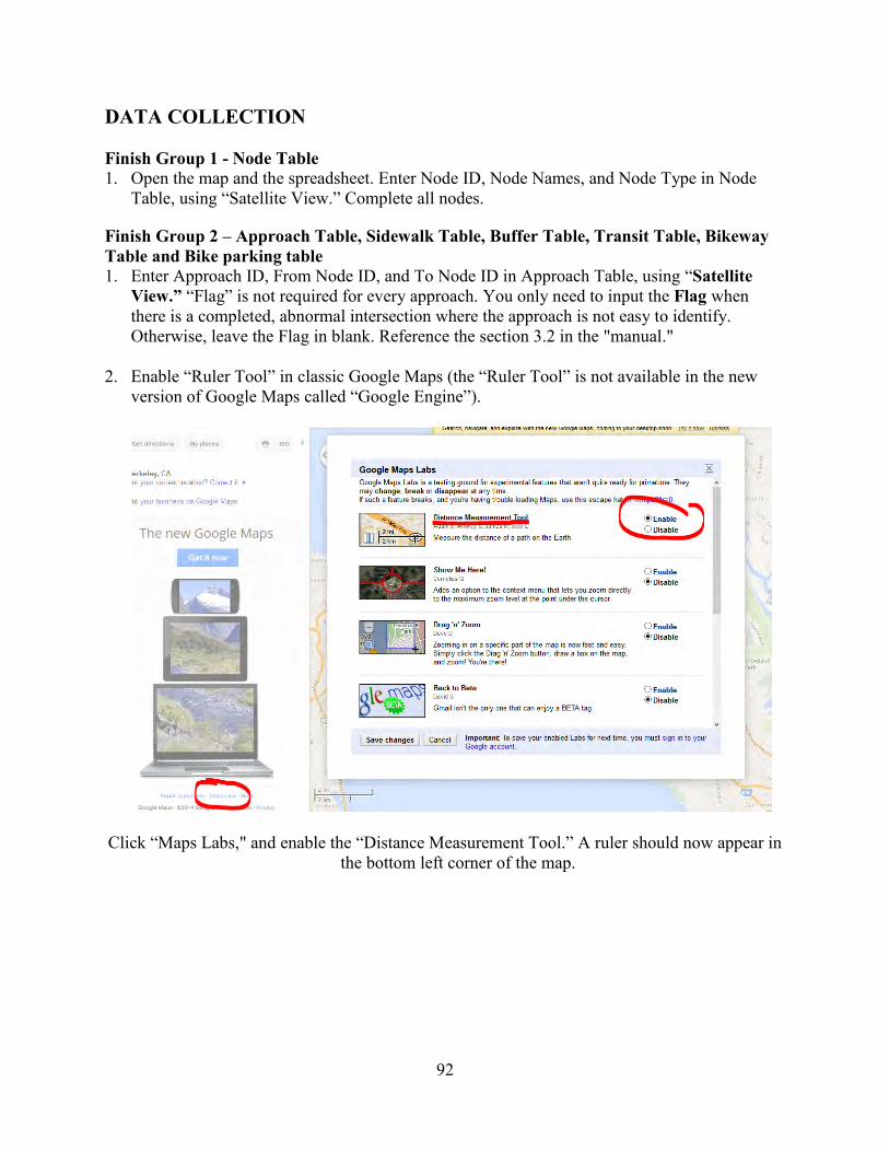
92

DATA COLLECTION Finish Group 1 - Node Table 1. Open the map and the spreadsheet. Enter Node ID, Node Names, and Node Type in Node

Table, using “Satellite View.” Complete all nodes.

Finish Group 2 – Approach Table, Sidewalk Table, Buffer Table, Transit Table, Bikeway Table and Bike parking table 1. Enter Approach ID, From Node ID, and To Node ID in Approach Table, using “Satellite

View.” “Flag” is not required for every approach. You only need to input the Flag when there is a completed, abnormal intersection where the approach is not easy to identify. Otherwise, leave the Flag in blank. Reference the section 3.2 in the "manual."

2. Enable “Ruler Tool” in classic Google Maps (the “Ruler Tool” is not available in the new

version of Google Maps called “Google Engine”).

Click “Maps Labs," and enable the “Distance Measurement Tool.” A ruler should now appear in the bottom left corner of the map.

93

3. Using “Satellite View,” traverse the route once, gathering parking lane width, sidewalk width, bikeway width, and buffer width (the orange variables in the group 2 tables) for each approach using the ruler tool. NOTE: When measuring distance, make sure “45 degree” mode is enabled to ensure consistent measurements.

4. Using a split-screen “Street View” and “Satellite View” (see image below). Drag the “Street view” icon on the map to activate street view.

94

In the “Street View” mode, click the arrow icon in small box of satellite view on the bottom left corner.

The split-screen will then be displayed as below.

95

5. Traverse the route once in a direction of traffic flow, gathering transit, signage, and bike parking for the approaches along the traffic flow.

Navigate by clicking in the “Street View” to avoid missing data.

The “Satellite View” must be on one of the 3 most zoomed in views in order to see the transit symbols that Google has already marked. Use those symbols as a check. They do NOT consistently capture every transit; however, if there is a symbol, it’s probably correct.

6. Using the same setup as in step 1 and 2, traverse the route in the OPPOSITE direction. Collect transit, signage, and bike parking on this side of the road.

Finish Group 3 – Crosswalk Table 1. Use a split-screen of “Street View” and “Satellite View.” Go through the route in

increasing node order. At each node except for the first and the last, determine the number of crosswalks associated (or around) that node, and complete that number of rows in the Crosswalk N_ID section with that node's ID. Then, fill out A_ID_1 and A_ID_2.

2. After labeling the crosswalks, collect the rest of the data. Use the ruler in “Satellite View” to

collect crossing distances, and the “Street View” for other information. Note that the Street View images and Satellite View images may be different because the pictures may have been taken at different times. Defer to the more recent picture; this is usually Satellite View. In such a case, it is often difficult/ impossible to collect other data such as Pedestrian Signal Light presence. Leave these fields blank.

3. Repeat steps 1 and 2 for the next node.

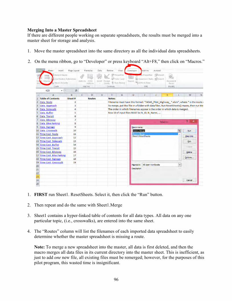
96

Merging Into a Master Spreadsheet If there are different people working on separate spreadsheets, the results must be merged into a master sheet for storage and analysis. 1. Move the master spreadsheet into the same directory as all the individual data spreadsheets.

2. On the menu ribbon, go to “Developer” or press keyboard “Alt+F8,” then click on “Macros.”

1. FIRST run Sheet1. ResetSheets. Select it, then click the “Run” button.

2. Then repeat and do the same with Sheet1.Merge

3. Sheet1 contains a hyper-linked table of contents for all data types. All data on any one particular topic, (i.e., crosswalks), are entered into the same sheet.

4. The “Routes” column will list the filenames of each imported data spreadsheet to easily determine whether the master spreadsheet is missing a route. Note: To merge a new spreadsheet into the master, all data is first deleted, and then the macro merges all data files in its current directory into the master sheet. This is inefficient, as just to add one new file, all existing files must be remerged; however, for the purposes of this pilot program, this wasted time is insignificant.

97

User Testing Feedback This memo reports on feedback received from Caltrans staff on the data collection procedures for pedestrian and bicycle infrastructure being developed under SHSP 08.09. SHSP 08.09 includes constructing a database format for pedestrian and bicycle infrastructure and volume data to be collected across the state highway network, developing a preferred data collection plan to populate this database, and conducting a pilot data collection effort on 100 miles of state highway to ensure that the data collection procedures work properly. During the project, the research team was asked to create a small testing package for Caltrans staff to work with in order to ensure that the data collection process works properly given institutional constraints, and to allow the staff to lend their expertise regarding matters of state highway infrastructure characteristics.

Based on expert user testing, a number of comments were received for consideration in finalizing the data collection process and writing the final report for the project. These comments can be grouped into three broad categories:

User interface redesign suggestions Data collection process questions Data collection suggestions

The various questions and comments that were received are paraphrased below, including

responses from the research team. Overall, response from the expert users was favorable, and it appears that with refinement of the data collection system, Caltrans staff would be open to collecting this data.

User Interface Redesign Suggestions A number of comments received were complaints specifically directed at the time measurement spreadsheet. This tool is only being used during the data collection pilot to estimate how long it takes to collect data, and will not be used in long term data collection. The following comments were received on this topic:

The time tracking spreadsheet does not like dragging to fill cells, but if you have ten 4-way nodes in a row, you’d have to be crazy to type them all in individually.

Having to go back and forth between the different maps and spreadsheet and stop watch is time costly and can cause confusion during the process.

The stopwatch malfunctioned half way into the process. Many of the problems of the spreadsheet timer program malfunctioning will be

eliminated either by using a simple spreadsheet (without a timer running in the background), or by switching to a more sophisticated data recording method.

Multiple comments regarding the data recording and storage mechanism were made. The two biggest themes were that a GIS-based approach should be considered, and that duplicate records should be set to auto-populate so as to lessen the data entry burden.

Switching the data collection method to a GIS solution (from the current combination of MS Excel paired with Google Maps in a web browser) offers some substantial advantages and disadvantages. This approach would be advantageous in that it would retain geographical information on the infrastructure and volume characteristics being collected, and that length attributes (e.g., of sidewalk and crosswalk elements) could be automatically calculated. There is also a primary step in the data collection process during which approaches and nodes must be

98

manually drawn and identified in a Google Maps layer, which could potentially be automated based on an existing GIS file of the highway network. Finally, any data collected based on overhead imagery (e.g., facility widths, crosswalk types) could be collected and recorded within the GIS software.

One disadvantage of the GIS approach is that while it would integrate the data recording process with the data collection process for overhead imagery-based elements, anything that requires street level views would still have to be collected in Google Maps. The inefficiencies of switching between two windows to collect and record the data would persist. Additionally, one argument in favor of a GIS approach is that it might be less subject to network lag than use of a set of web hosted imagery such as Google. However, this improvement is far from certain, as GIS software also tends to lag. Finally, GIS software is not quite as ubiquitously available as the combination of MS Excel and a web browser, nor are the skills required to operate it, so this switch might limit the ability of new users (e.g., interns) to adapt to the data collection process quickly and contribute to documenting the entire highway network.

The other major user interface improvement that was requested was an auto-population ability for any duplicate records or sequentially numbered elements. For example, the approach IDs tend to be entered in a sequential order. This was not implemented originally because there is no requirement that approaches be sequential, and so user consideration is needed to ensure that the approach being described is correctly identified (rather than losing track of what one is doing and overlooking these details). One way in which we envision this being improved upon is switching to form-based data entry after shifting to a relational database. Alternatively, this would be less of an issue in a GIS database because spatial relationships would be explicitly defined by element locations, rather than by ID numbers. This could be implemented either in standalone GIS software or within Google Maps. Data Collection Process Questions The second overall set of user feedback was questions pertaining to the data collection process. In particular, a number of specific instances were identified in which the data collector was unsure of how to classify a piece of infrastructure. These include the following, which are followed in italics by the research team’s responses:

Do driveways across from named roads count as approaches? Can you have a 4-way node with only three approaches? (i.e., http://goo.gl/maps/la9HD ) No, driveways should not be classified as approaches.

Sidewalk width can be affected by café tables and other fixtures located immediately outside buildings in business areas. Address in manual. (http://goo.gl/maps/AI2aM) What about permanent/semi-permanent furniture/landscaping/stairs against buildings? It is sometimes hard to tell where the front edge of a building is (i.e. where the edge of the edge of the sidewalk is) (http://goo.gl/maps/eHPuk). For these cases, the data collection manual suggests that the data collector is to measure the width of the facility at a “representative” location. Generally, what should be measured is the clear width in the presence of obstructions like café furniture.

Unpaved sidewalk? How does this get classified? (http://goo.gl/maps/Byh5A) This should be classified as a sidewalk and measured as such.

99

It is hard to divide park lane from travel lane when there is no stripe. (http://goo.gl/maps/NGXr9) In cases like this, the data collection team has been using a standard of an 8’ parking lane, which is based on field measurements taken in multiple locations on Highways 123 and 13 in Berkeley. The data collection manual will be updated accordingly.

Also, should park lane width variable be used for shoulder width where parking is not allowed? (http://goo.gl/maps/ZG2Ve) No. Shoulder width is already documented in the existing TASAS database.

If there is a median, but it ends before the crosswalk, I did not consider it a “refuge.” (http://goo.gl/maps/MjlDO) That is the correct classification.

In addition to these infrastructure-specific questions, the following more general

questions/comments were made regarding the data collection process: If you miss a node while generating the identifiers or the road changes in the future, what

is the best way to go back and re-number the approaches? Consider the system used for postmiles where prefixes for revised routes. Rather than using a prefix system, the approach ID system used here does not rely on sequential numbering (like the PM system), so any missed elements can be identified using a value from later in the series. The spatial relationships of the system are made by relational identifiers between approaches and nodes.

Measuring distances such as parking distances is difficult and in some cases and impossible from Google Maps on one side of streets when viewing from satellite view in the split screen mode. This has been encountered by the research team as well, particularly in cases where the angle of the imagery is such that buildings obscure the sidewalk next to them. A field has been added to the database to denote uncertainty with a particular measurement, and data collectors will be instructed to make their best estimate based on prevailing conditions around the obscured site and based on the pieces of the infrastructure that are visible.

Data Collection Suggestions Finally, the following comments were received about particular improvements or corrections that could be made to the data collection process.

I believe the 45o view to be less accurate for measuring. Switching back to 90o, I can see that the perspective encouraged me to misplace the ends of my measurement line. The data collection team believes that this is simply an artifact of switching between views with the pins kept in the same place. Measuring using both methods was tested at a number of locations and compared with field validation, and the 45o and 90o measurements were typically within +/- 1 foot of each other.

I sometimes have network issues that make Google Maps very slow to update.

100

One potential solution to this problem that was brought up during the Quarterly Meeting was using imagery that Caltrans has hosted locally at some or all districts. The research team does not know the details of this data set, but it sounds as if it can be accessed via the local area network rather than relying on the internet connection, which appears to be the problem resulting in slow updating.

Data collection for crosswalks needs to be more specified and include non-marked crosswalks since there are ADA ramps at corner of these of intersections. The data collection manual has been updated to include unmarked crosswalks.

In the user manual, please refer to ADA ramps descriptions used by Caltrans and not from other DOTS such as the one on page 34. The data collection manual has been updated to reflect the language in the Caltrans Standard Plans regarding curb ramps.

Based on the comments received in this user testing, the data collection manual for the proposed TASAS database addition has been revised. The Caltrans employees who participated in the user testing both seemed to be generally satisfied with the process, and with refinement it appears that the database can be populated and updated periodically by novice users which, once complete, will serve as a useful resource in conducting statewide assessments of pedestrian and bicyclist risk based on infrastructural characteristics.

101

APPENDIX 5. FIELD DATA COLLECTION PACKET

HWY #: __ _ TASAS Field Data Collect ion Form- Approaches Data Collector: ______ _

Approach Sidewalk Buffer Transit Bikeway Width

ID Flag Informal Parking Width Obstructions Parking Width Type Color Crossings Lane (u/p)

W idt h

d p np nm y N sh bl bbl na u p

d p np nm y N sh bl bbl na u p

d p np nm y N sh bl bbl na u p

d p np nm y N sh bl bbl na u p

d p np nm y N sh bl bbl na u p

d p np nm y N sh bl bbl na u p

d p np nm y N sh bl bbl na u p

d p np nm y N sh bl bbl na u p

d p np nm y N sh bl bbl na u p

Time: Beginning cross street:

HWY#· TASAS Field Data Collection Form Crosswalks - Data Collector·

ID Node App. App. Style Curb Truncated Crossing Color Ped. Ped. Median Advanced Condition ID ID_1 ID_2 Ramp Dome Distance Signal Signal Refuge St op

Type Color Head Button Width

pa on y 0 n wyd o y N y N sb ay n 1 2 3

p ao n y 0 n wy do y N y N sb ay n 1 2 3

pa o n y 0 n wy d o y N y N sb ay n 1 2 3

p ao n y 0 n wydo y N y N sb ay n 1 2 3

p ao n y 0 n wy d o y N y N sb ay n 1 2 3

pa on y 0 n wy d o y N y N sb ay n 1 2 3

pa o n y 0 n wy do y N y N sb ay n 1 2 3

p aon y 0 n wy d o y N y N sb ay n 1 2 3

p ao n y 0 n wy d o y N y N sb ay n 1 2 3

pa on y 0 n wy d o y N y N sb ay n 1 2 3

pa o n y 0 n wy d o y N y N sb ay n 1 2 3

pa o n y 0 n wy do y N y N sb ay n 1 2 3

Time: Beginning cross street :

102

HWY#: TASAS Field Data Collection Form - Signage Data Collector: ______ _

ID App. MUTCD ID App. MUTCD ID App. MUTCD Time: ID Number ID Number ID Number Beginning cross street :

Legend

Description CA-MUTCD Number

Pedestrian Warning Wll-2 Bicycle Warning Wll-1 No Pedestrian Crossing, Use R49A Crosswalk No Pedestrian Crossing R9-3/9-3bP (symboi)/Use Crosswalk No Bicycles R5-6 Yield Here to R1-5/R1-5a Pedestrians/Peds In-Street Ped Crossing R1-6/R1-6a No Pedestrians, Bicycles, R5-10a,b, c Motor-Driven Cycles/No Pedestrians or Bicycles/No Pedestrians Share the Road (plaque) W16-1P Turning Vehicles Yield to R10-15 Peds Other Pedestrian Sign age Other Ped Other Bicycle Sign age Other Bike

Field Data Collection Directions -Approaches

10: approach 10, directly f rom map Bikeway Width: Measure the width of the bikeway. This will often be

Flag: Note if approach is a special type with "ghost", " triangle", "offset", or 110ther".

Informal Crossing: Options are "demonstrated", " passable", "not passable", and "no median". Demonstrated means there are visible signs of informal crossings (e.g. people doing it, worn paths in planters, etc.).

Parking l ane Width: Measure with measuring wheel from curb to marked edge of parking lane (T designs on road), bike lane edge or effective edge if others do not exist. If none, mark "0".

Sidewalk Width: Measure f rom edge of buffer zone to building frontage at a roughly representative point using the measuring wheel. If none, mark "0".

Sidewalk Obstructions: Note any obstruct ions (with a brief description) in the sidewalk that reduce the passable width to below 3' at any points, or below 4' for sustained distances.

Buffer Width: Measure the width of the buffer zone from the curb to the sidewalk. In cases with tree wells, this will be to the edge of the tree well. If none, mark "0".

Transit : Record if there are any transit stops along the approach. (1/0)

Bike Parking: Count the number of bicycle racks along the approach. If none, mark "0".

the width of a bicycle lane. If none, mark "0".

Bikew ay Type:

~

A shared

bike lane

Bikeway Color: unpainted or painted.

Example Street

section widths

---

buffered bike lane

103

Field Data Collect ion Directions- Crosswalks

ID: Arbitrary index for the crosswalk.

Node ID: Identifies the node where the crosswalk is located.

Approach IDs: Two approaches that define the crosswalk's location. See data collection manual for more specific directions.

Style: The crosswalk design categories to be recorded are as follows :

Sol Std Cont Dsh Zeb Ldr Tri4

Curb Ramp Type: The possibilities for this field are perpendicular (facing directly at crosswalk), apex("on t he 45 degree" of the corner), other and none. If the curb ramp is only present on one side of the crosswalk, mark "none".

Truncated Dome Color: Mark whether the truncated domes (small bumpy surface at the curb) are yellow, some other color, or not present. If domes are only present on one side of the crosswalk, mark "none".

Crossing Distance: Measure from curb to curb on the side of the crosswalk away from the intersection, along the painted line.

Color: Possible options for the crosswalk paint color are w hite, yellow, decorative pavers, and other.

Pedestrian Signal Head: Mark whether pedestrian signal heads are present. If they are not on both sides of the crosswalk, mark No.

Pedestrian Signal Button: Mark whether pedestrian signal call buttons are present on both sides of the crosswalk.

Median Refuge Width: Measure the width of the median refuge island. If one is not present, record this as "0".

Advanced Stop: Ind icate whether an advanced yield or stop warning is given for cars approaching this crosswalk. The possibilities here are stop bar, advanced y ield, and neither.

Stop bar Advanced~ Yield ~~~~~~~

Condition: Rank the condition of the crosswalk paint on a 1-3 scale, where 1 is freshly painted and 3 is heavily worn or faded.

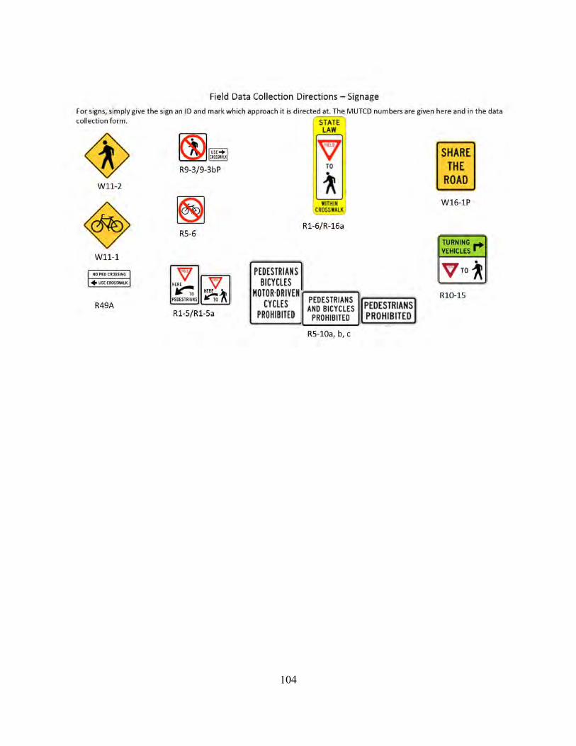
104

Field Data Collection Directions- Signage

For signs, simply give the sign an ID and mark which approach it is directed at. The MUTCD numbers are given here and in the data collection form. STATE

Wll-2

Wll-1

R49A

1~1 USEo+

CROS!111ll

R9-3/9-3bP

R5-6

1'1:1 ~ 11~~ HERE v ~ HERE AI

PEDESTRIANS ~. f\

R1-5/R1-5a

PEDESTRIANS BICYCLES

MOTOR·DRIVEN CYCLES

PROHIBITED

LAW

vv TO •

1\ WITHIN

CROSSWALK

R1-6/R-16a

L_ :~g~~~~~LNE~ PEDESTRIANS I

PROHIBITED PROHIBITED --

R5-10a, b, c

SHARE THE

ROAD

W16-1P

TURNING_. VEHICLES I~

• Vro~

R10-15

105

APPENDIX 6. TIME-ESTIMATION SPREADSHEET TOOL We have developed an Excel macro to use for storing measurements and timing the data collection process. An image of this spreadsheet is shown in Figure A-1.

Figure A-1. Screenshot of Macro Tool

The instructions on how to use this macro are shown at the top of the sheet. For example, when collecting data on a given approach’s sidewalks, follow the steps below:

1. Click the “Start” button (circled in red). 2. Switch to the web browser and conduct the data collection as detailed in the “Sidewalk”

section below. 3. Enter the measurements in the spreadsheet. 4. The time cost will be automatically recorded in a separate sheet titled “time cost.” 5. Proceed to the next element. 6. Click the “Stop” button when you need to close the Excel file. Click the “Break” button

when you leave the Excel file opened and take a break. Then click the “Resume” button to re-start.

Conduct this same process for each of the elements across the selected segments on the highway network. The order of elements to be measured is as follows: Finish “Node Table,” labeled as “Group 1” in the spreadsheet. Finish “Approach Table” to “Signage Table,” labeled as “Group 2” in the spreadsheet. Finish “Crosswalk Table,” labeled as “Group 3”

Start/stop button Break/resume button Instructions