Embed Size (px)
Citation preview

MISCELLANEOUS PAPER S-73-1
STATE-OF-THE-ART FOR ASSESSING EARTHQUAKE HAZARDS IN
THE UNITED STATES Report 24
WES RASCAL CODE FOR SYNTHESIZING EARTHQUAKE GROUND MOTIONS
by
Walter J. Silva
with program coding by
Kin Lee
Pacific Engineering and Analysis El Cerrito, CA 94530
May 1987
Report 24 of a Series
Approved For Public Release; Distribution Unlimited
Prepared tor DEPARTMENT OF THE ARMY US Army Corps of Engineers Washington, DC 20314-1000
Under Contract No. DACW39-85-M-1585
Monitored by Geotechnical Laboratory US Army Engineer Waterways Experiment Station PO Box 631, Vicksburg, Mississippi 39180-0631

T -----------------·-I
Unclassified SECURITY CLASSIFICATION OF THIS PAGE
REPORT DOCUMENTATION PAGE I Form Approved
OM8 No 0704-0188 Exp. Date Jun JO. 1986
la. REPORT SECURITY CLASSIFICATION 1 b. RESTRICTIVE MARKINGS Unclassified
2a. SECURITY CLASSIFICATION AUTHORITY 3. DISTRIBUTION/ AVAILABILITY OF REPORT Approved for public release; distribution
2b. DECLASSIFICATION/ DOWNGRADING SCHEDULE unlimited
4. PERFORMING ORGANIZATION REPORT NUMBER(S) 5. MONITORING ORGANIZATION REPORT NUMBER(S)
Miscellaneous Paper S-73-1
6a. NAME OF PERFORMING ORGANIZATION 6b. OFFICE SYMBOL 7~siit~fE:~F MONITORING ORGANIZATION
Woodward-Clyde Consultants (If applicable)
Geotechnical Laboratory 6c. ADDRESS (City, State, and ZIPCode) 7b. ADDRESS (City, State, and ZIP Code)
Walnut Creek, CA 94596-3564 PO Box 631 Vicksburg, MS 39180-0631
Ba. NAME OF FUNDING/ SPONSORING Bb. OFFICE SYMBOL 9. PROCUREMENT INSTRUMENT IDENTIFICATION NUMBER ORGANIZATION (If applicable)
US Army Corps of Engineers Contract No. DACW39-85-M-1585 Sc. ADDRESS (City, State, and ZIP Code) 10. SOURCE OF FUNDING NUMBERS
PROGRAM PROJECT TASK WORK UNIT Washington, DC 20314-1000 ELEMENT NO. NO. NO. ACCESSION NO.
11. TITLE (Include Security Classification) STATE-OF-THE-ARl t-UR ASSt.::iSING Ef\K rHQUAKE H IZARDS IN 11 UNllt.U STATES; Report 24: WES RASCAL Code for Synthesizing Earthquake Ground Motions
12. PERSONAL AUTHOR(S)
Silva, Walter J., Lee, Kin 13a. TYPE OF REPORT 113b. TIME COVERED
Report 24 of a Series FROM To
14. DATE OF REPORT (Year, Month, Day) rs. PAGE COUNT
May 1987 120 16. SUPPLEMENTARY NOTATION
Available from National Technical Information Service, 5285 Port Royal Road, Springfield, Virginia 22161.
17. COSA Tl CODES 18. SUBJECT TERMS (Continue on reverse if necessary and identify by block number)
FIELD GROUP SUB-GROUP Computer programs (LC) RASCAL (Computer Earthquake engineering (LC) program) (LC)
19. ABSTRACT (Continue on reverse if necessary and identify by block number) A computer code (RASCAL) has been developed to provide realistic predictions of ground
motion parameters for applications to earthquake engineering risk assessment. The code incorporates random vibration theory (RVT) to calculate peak value of acceleration and velocity in addition to response spectra for specified earthquake source and propagation path parameters (Boore, 1983). To generate synthetic time histories, the code combines the phase spectra from observed strong motion records to a theoretical Brune (1970, 1971) modulus. In addition, the above techniques are employed to produce an acceleration time history whose response spectrum matches a specified target or design response spectrum.
20 DISTRIBUTION/ AVAILABILITY OF ABSTRACT 21. AffiTR,CT SE.Cf!l1Td CLASSIFICATION IXJ UNCLASSIFIED/UNLIMITED 0 SAME AS RPT. 0 DTIC USERS nc ass1 1e
22a. NAME OF RESPONSIBLE INDIVIDUAL 22b. TELEPHONE (Include Area Code) I 22c_ OFFICE SYMBOL
DD FORM 1473,84MAR 83 APR edition may be used until exhausted.
All other editions are obsolete. SECURITY CLASSIFICATION OF THIS PAGE
Unclassified

Unclassified SECURITY CLASSIFICATION OF THIS PAGE
REPORT DOCUMENTATION PAGE I Form Approved
0MB No 0704-0188 Exp Date Jun 30, 1986
la. REPORT SECURITY CLASSIFICATION lb. RESTRICTIVE MARKINGS Unclassified
2a SECURITY CLASSIFICATION AUTHORITY 3. DISTRIBUTION I AVAILABILITY OF REPORT Approved for public release; distribution
2b. DECLASSIFICATION/ DOWNGRADING SCHEDULE unlimited
4. PERFORMING ORGANIZATION REPORT NUMBER(S) 5. MONITORING ORGANIZATION REPORT NUMBER(S) Miscellaneous Paper S-73-1
6a. NAME OF PERFORMING ORGANIZATION 6b. OFFICE SYMBOL 7~s1t~tE~F MONITORING ORGANIZATION Woodward-Clyde Consultants (If applicable)
Geotechnical Laboratory 6c. ADDRESS (City, State, and ZIP Code) 7b. AODRESS (City, State, and ZIP Code)
Walnut Creek, CA 94596-3564 PO Box 631 Vicksburg, MS 39180-0631
Sa. NAME OF FUNDING/ SPONSORING Bb. OFFICE SYMBOL 9. PROCUREMENT INSTRUMENT IDENTIFICATION NUMBER ORGANIZATION (If applicable)
US Army Corps of Engineers Contract No. DACW39-85-M-1585 Be. ADDRESS (City, State, and ZIP Code) 10. SOURCE OF FUNDING NUMBERS
PROGRAM PROJECT TASK WORK UNIT Washington, DC 20314-1000 ELEMENT NO. NO. NO. ACCESSION NO
11. TITLE (Include Security Clauification) STATE-OF-THE-ART FUR ASSESSING E \K ltiQUAKE HHZJ!.RDS TN I~ I:. 1JN1 I tu STATES; Report 24: WES RASCAL Code for Synthesizing Earthquake Ground Motions
12. PERSONAL AUTHOR(S) Silva, Walter J., Lee, Kin
13a. TYPE OF REPORT 113b. TIME COVERED Report 24 of a Seri es FROM To
14. DATE OF REPORT ( Year, Month, Day) T 5 PAGE COUNT May 1987 120
16. SUPPLEMENTARY NOTATION Available from National Technical Information Service, 5285 Port Royal Road, Springfield, Virginia 22161.
17. COSATI CODES 18. SUBJECT TERMS (Continue on reverse if neceuary and identify by block number)
FIELD GROUP SUB-GROUP Computer programs (LC) RASCAL (Computer Earthquake engineering (LC) program) (LC)
19. ABSTRACT (Continue on reverse if neceuary and identify by block number)
A computer code (RASCAL) has been developed to provide realistic predictions of ground motion parameters for applications to earthquake engineering risk assessment. The code incorporates random vibration theory (RVT) to calculate peak value of acceleration and velocity in addition to response spectra for specified earthquake source and propagation path parameters (Boore, 1983). To generate synthetic time histories, the code combines the phase spectra from observed strong motion records to a theoretical Brune (1970, 1971) modulus. In addition, the above techniques are employed to produce an acceleration time history whose response spectrum matches a specified target or design response spectrum.
20. DISTRIBUTION/ AVAILABILITY OF ABSTRACT 21 A~STRtCT SE~f!ITd CLASSIFICATION IXJ UNCLASSIFIED/UNLIMITED 0 SAME AS RPT. 0 DTIC USERS nc ass, ,e
22a. NAME OF RESPONSIBLE INDIVIDUAL 22b TELEPHONE (Include Area Code) 22c. OFFICE SYMBOL
DD FORM 1473, 84MAR 83 APR ed1t1on may be used until exhausted. All other editions are obsolete.
SECURITY CLASSIFICATION OF THIS PAGE Unclassified

PREFACE
This report was prepared by Dr. Walter J. Silva of Woodward-Clyde Associates, Walnut Creek, California, under Contract No. DACW39-85-M-1585. Program coding for the report was done by Mr. Kin Lee of Woodward-Clyde. The study is part of ongoing work at the US Army Engineer Waterways Experiment Station (WES) in the Civil Works Investigation Study, "Earthquake Hazard Evaluations for Engineering Sites," sponsored by the Office, Chief of Engineers (OCE), US Army.
Preparation of this report was under the direct supervision of Dr. E. L. Krinitzsky, Engineering Geology and Rock Mechanics Division (EGRMD), Geotechnical Laboratory (GL), WES, and the general supervision of Dr. D. C. Banks, Chief, EGRMD, and Dr. W. F. Marcuson III, Chief, GL.
COL Allen F. Grum, USA, was the previous Director of WES. COL Dwayne G. Lee, CE, is the present Commander and Director. Dr. Robert W. Whalin is Technical Director.

CONTENTS
Page
PREF ACE. . . . . . . . . . . . . . . . . . . . . . . . . . . . . . . . . . . . . . . . . . . . . . . . . . . . . . . . . . . . . l
1.0 INTRODUCTION................................................... 3
2.0 APPROACH....................................................... 7
2. l Model .................................................. ,. . . 7
3.0 OBJECTIVE...................................................... 10
4.0 RESULTS........................................................ 11
4.1 Prediction and Synthesis Capability....................... 11 4.2 Response Spectral Scaling Capability...................... 14
5.0 CONCLUSION AND RECOMMENDATIONS................................. 17
5.1 Conclusion................................................ 17
6. 0 MATHE MA TI CAL DEVELOPMENT. • . . . . . . . . . . . . . . . . . . . . . . . . . . . . . . . . . . . . . 18
7. 0 USER MANUAL. . . . . . . . . . . • . . . • . . . . . . . . . . . . . . . . . . . . . . . . . . . . . . . . . . . . 28
7.1 Prediction Methodology.................................... 28 7. 2 Synthesis Methodo 1 ogy. . . . . . . . . . . . . . . . . . . . . . . . . . . . . . . . . . . . . 28 7.3 Response Spectral Scaling Methodology..................... 29 7.4 User 1 s Guide.............................................. 31 7.5 Program Listing........................................... 36
REFERENCES ....••. ;.................................................. 71
TABLES 1-4
FIGURES 1-12
2

1.0 INTRODUCTION
In either a deterministic or probabilistic seismic hazard evaluation an
essential element is a description of the variability of ground motion parameters with distance (or depth) and earthquake size or magnitude. Once a distance and design basis earthquake is decided upon, the region
specific attenuation relation is then utilized as an estimator to predict,
with associated variance, the ground motion parameters to be expected at the site. If attenuation relations are available which parameterize peak
values and frequency content through the response spectra, then the exposure is reasonably well specified. If however, only peak values are constrained by the attenuation relation, these may be utilized to scale an
assumed frequency dependence via an adopted response spectrum shape.
While not as satisfying as a region specific response spectrum shape, the adopted shapes are based upon many observations and can be adjusted to relect the magnitude range contributing to the seismic hazards.
The representation of the design ground motions by a response spectrum is
sufficient for the seismic design evaluations of most engineered
structures (e.g. commercial buildings, hospitals, etc.). However, for
large, complex and/or critical facilities, time history analyses are often
necessary, especially when there is significant non-linear structural
response (e.g. earth dams, offshore platforms, etc.). For these
evaluations, one or more accelerograms are selected whose response spectrum match the design spectrum in some average sense.
In regions of high seismicity rates which have had established strong
motion instrumentation programs for a period of time, a sufficient data
base of observations may be available to provide representative
accelerograms and to constrain regression analyses for peak values and
response spectra. While the range of magnitudes and distances is always
less than ideal, definite trends may be characterized statistically so
that extrapolations may be made with some level of confidence in not only the values themselves but also the degree of conservatism as well.
3

Time histories, which are consistent in amplitude, duration, and frequency content with observational data are generated through filtering noise samples (Nau et al., 1982) or by splicing together selected portions of observed time histories. Also, response spectral matching techniques may be applied to empirical data which scale, through filters, the time history (Tsai, 1972). This results in a time history whose response spectra is close to the design response spectrum.
Although these approaches retain the frequency, amplitude, and duration characteristics in a statistical sense, they usually produce time histories which could not have resulted from any earth process. The resulting velocity and displacement time histories from the artificially generated accelerograms are often inconsistent with observed motions, a fact that may be essential in response calculations for longer period structures. These approaches have evolved through necessity and employ little knowledge of earthquake source processes or wave propagation physics.
At the other extreme in ground motion prediction, detailed descriptions of source properties (e.g. location, direction, rupture velocity, distribution of asperities or barriers, and rise times) and propagation path parameters are utilized to generate synthetic time histories (Heaton and Helmberger, 1978, Apsel et al., 1983). These models are essential to understand past seismic events and they can be utilized to predict future ground motions. However, they require the specifications of source details and path effects which can have profound effects on the predicted ground motion. Generally, a range in parameters is utilized in a sensitivity analysis which translates into uncertainties in the predicted motion.
The modeling approach has recently attempted to accommodate, in a natural way, some of the stochastic aspects of source processes and path effects by utilizing small, well recorded events as a basis to construct time histories (Hartzell, 1978). The observed events are scaled and summed, utilizing source physics, to model time histories for large events (Hadley
4
and Helmberger, 1980; Kanamori, 1979). This hybrid approach is very
attractive in that aspects of both source and path complexities are
incorporated. This reduces somewhat the arbitrary nature in parameter
specification and allows more definitive calibrations with large events to help constrain the remaining variables.
An extremely important application of the hybrid approach is its utility
in providing guidelines in extrapolations. Estimates of ground motion parameters using various empirical models (Donovan, 1973; Idriss, 1978; Joyner and Boore, 1981; Campbell, 1981; Joyner and Boore, 1982; Joyner and
Fumal, 1984) differ little in regions of distance and magnitude where data
are abundant. However, in regions where extrapolations are required, close to moderate and large earthquakes, the differences can be large. The differences are due primarily to the mathematical form chosen to
parameterize the data. In these regions, the careful use of modeling
which is based upon observational data can be a powerful tool in assessing the conservatism of extrapolated empirical relations (Hadley and
Helmberger, 1982). The modeling is calibrated in regions where data exist
by parameter variation and sensitivities are assessed. A level of
confidence is achieved, at least by the modelers, and estimates are made
on ground motion which may guide or give confidence in extrapolated
empirical relations.
While the above techniques are the basic tools in ground motion
estimation, they are both fundamentally based upon observational data. The empirical approach obviously cannot be utilized with few strong motion
data, while the analytical and hybrid techniques utilize data either
directly or at least for calibration purposes to constrain free parameters.
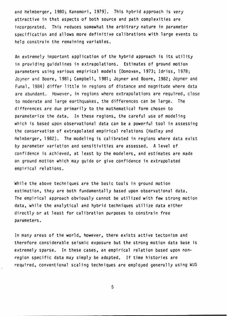
In many areas of the world, however, there exists active tectonism and
therefore considerable seismic exposure but the strong motion data base is
extremely sparse. In these cases, an empirical relation based upon non
region specific data may simply be adopted. If time histories are required, conventional scaling techniques are employed generally using WUS
5

acceleration data. The justification primarily relies upon arguments
considering similar tectonic environments, crustal structure, style of
faulting, depth of events, observed attentuation of shaking intensity and other less tangible aspects generally referred to as engineering judgement. While this methodology is an accepted practice by necessity,
an approach is needed which does not rely upon strong motion data for
calibration but rather only for confirmation.
6

2.0 APPROACH
Another approach, which utilizes simple earthquake source theory and wave propagation physics, has recently demonstrated great promise in circumstances such as these {Boore, 1983; Atkinson, 1984, McGuire et al., 1984). The basic advantage lies in using weak motion indirectly to predict strong motion. The weak motion is due to small magnitude {generally less than Mw = 5) local or regional events. These data, from both analogue and digital recordings, are used to estimate region specific source and wave propagation parameters. Those parameters are then input to the source and propagation models which predict the motion due to events at distances and from source sizes for which no data exist. This approach employs random vibration theory {RVT) applied to a Brune source spectrum {Brune; 1970, 1971) to characterize strong ground motion. While this approach is not perfect, and some problems remain, we believe that, based upon its recent success {Boore, 1983; Atkinson, 1984, McGuire et al., 1984) and our preliminary results, it will prove to be quite useful.
2.1 Model
The formalism employed to develop an attenuation relation with little or no strong motion data is based upon a simple theoretical model of the earthquake process and wave propagation physics. The theoretical basis was developed and calibrated with observed data by Hanks and McGuire (Hanks, 1979; McGuire and Hanks, 1980; Hanks and McGuire, 1981). They used the Brune {1970, 1971) spectrum to model root mean square {RMS) acceleration as a function of magnitude and distance for stiff {rock) sites. To model peak values, they utilized results from random vibration theory to relate the RMS predictions to maximum values. Boore {1983) has extended the range of applications to include predictions of peak horizontal velocities, Wood-Anderson seismographic response, and response spectra. Boore has also used this approach to generate synthetic acceleration time histories by employing random sequences whose spectra match the predicted Brune spectrum. The method leads to results which reproduce the empirical dependences of peak acceleration, peak velocity,
7

reproduce the empirical dependences of peak acceleration, peak velocity,
and pseudovelocity response spectral amplitudes on moment magnitude at
close distances. McGuire et al. (1984) further confirmed the results of
the RVT technique by demonstrating the close agreement between observed and predicted response spectral values. They also showed good agreement
between the calculated Brune spectrum and the acceleration spectral
density of empirical data for several discrete frequencies. In order to extend this approach to large distances, the model was modified to incorporate surface wave effects (Atkinson, 1984). At distances greater than about two crustal thickness (Herrmann, 1985), surface waves rather than shear waves, will carry the peak ground motion.
The technique developed in this study employs aspects of the above
developments to predict peak values (acceleration and velocity) and
response spectra. However it differs significantly from other techniques in the manner in which time histories are generated. These time histories
may be regarded as semi-empirical in that they use the Brune spectrum as a
modulus but an observed phase to generate the complex spectrum. The
advantage of this technique is that the non-stationarity, randomness, and
change in frequency with time is incorporated in a natural way.
Intergrations to velocity and displacement are then also more realistic.
The basic assumption with this technique is that the region-specific
source and wave propagation parameters are reflected primarily in the
spectral modulus. The phase spectrum accounts for the multipath effects
and surface wave contributions.
Since the RVT technique, employing a Brune spectrum, has demonstrated success in modeling both Western and Eastern United States data, the RVT
peak values (acceleration and velocity) are used to scale the time domain simulations. This is necessary since we are generally combining a modulus
and a phase which are somewhat incompatible. This arises because the
phase is from a time history with mixed phase properties while the Brune
spectrum is smooth (Pilant and Knopoff, 1970).
8

In order to preserve the magnitude dependency of strong motion duration
characteristics (Dobry et al., 1978) it is necessary to use a phase from a
record of approximately the same magnitude and distance as the design event. This arises because the phase spectrum determines how the energy
is distributed in time. The magnitude similarity is about~ one half unit of magnitude. The distance requirement on the phase is less
restrictive. Generally, we have found phases extracted from records within 20 to 25 km can be used for simulations from 10 to 30 km. Phases
from records at 40 to 50 km are used for distances greater than 30 km.
In cases where a time history is required when a target response spectrum
is specified, an initial Brune spectrum is generated based upon magnitude,
stress drop, and distance in addition to the region specific wave propagation parameters. The Brune spectrum is then scaled by taking
ratios of either, the RVT response spectra or a time domain response spectrum calculation, to the target response spectrum. The time domain
response spectrum is calculated from the synthesized time history. The
peak acceleration of the resultant time history is generally then scaled to the design value (which must be consistent with the target response spectrum).
9

3.0 OBJECTIVE
The original objective of this work was to develop a technique to generate a realistic time history whose response spectrum is compatible with a specified response spectrum. The plan was to use an observed time history and scale the modulus of its Fourier spectral density by the ratio of the observed response spectra to the target. The original phase would then be added to produce the desired time history. The process would be iterated until the response spectra of the scaled time history was close to the target response spectrum. However, in developing the code it was decided to abandon the observed modulus since the RVT technique had recently demonstrated such good results by employing the simple Brune spectrum. The most convincing evidence came from McGuire et al., (1984). They showed the effectiveness of the Brune spectra in predicting Fourier spectral density and response spectral values at close distances for several frequencies. By using a combined approach, that is a Brune modulus with an observed phase, it is possible to also incorporate all the predictive power of the RVT methodology. That is, in one code, the ability to predict peak acceleration, peak velocity, and response spectra in addition to generate realistic acceleration, velocity, and displacement time histories has been incorporated. This can be done for magnitudes from about 4 to 7 1/2 and from distances from 10 km to over 100 km. In addition a target response spectrum may be input to the code and an acceleration time history can then be generated whose response spectrum closely matches the target response spectrum.
10

4.0 RESULTS
Since the code, as it is presently configured, operates in two basic modes
depending upon whether or not a target response spectrum has been specified, the results section will be divided accordingly. The first section will address the predictive capability in terms of peak values for WUS and EUS tectonic environments. The time history synthesis will also be demonstrated. The second section will present the scaling results when
an input target response spectrum is specified.
4.1 Prediction and Synthesis Capability
In order to demonstrate the predictive characteristics of the code, results for both magnitude and distance scaling will be presented.
Magnitude scaling will include comparisons of peak acceleration and peak velocity at close distances with empirical relations for WUS and EUS
tectonic environments. Distance scaling will involve predicted peak acceleration vs distance for a single magnitude compared with empirical
data. Source and wave propagation parameters used for WUS and EUS predictions are shown in Table 1.
Figure 1 demonstrates the magnitude scaling for close distances (R<15 km) compared to three other attenuation relations: Joyner-Boore (1982) at 50% level, Seed and Schnable (1980), and Donovan (1973). The bars at
magnitudes 5 and 7 1/2 represent the scatter in the data base used by Joyner and Boore (1981). The lower magnitude variances are for the
Oroville aftershocks combining rock and soil sites (Shakal and Berneuter,
1980). All data are for distances of a few km to 15 km. Both the Joyner
Boore (1982) and Seed and Schnable (1980) curves are plotted for magnitude ranges over which the authors indicated the relations are valid. These relations are based upon WUS data. The Donovan (1973) curve, which is based upon world wide data, is plotted for the entire range since no discussion is given outlining the range of its validity. It should also
be pointed out that there are differences in definitions of distance which are significant at these close ranges. The calculated relation is based
11

upon a hypocentral distance of 10 km while the Joyner-Boore (1982) curve uses the closet distance to the surface projection of the fault. SeedSchnable (1980) and Donovan (1973) employ a "closest" distance. These differences in definition can easily result in differences of 0.2 to 0.3 log units at these close distances (Hanks and McGuire, 1981 ). The RVT predictions, which include the near site amplification factors (Boore, 1985), appears somewhat high but is generally within the 85% Joyner Boore (1982) curve (0.27 log units higher than the curve shown in figure 1). Also, for the higher magnitudes, 10 km is well within the source dimension which violates the far-field assumption in the Brune (1970, 1971) theory. With these considerations, we are favorably impressed with the results.
Peak particle velocities vs moment magnitude are plotted in Figure 2 for WUS parameters. Also shown is the empirical curve of Joyner and Boore (1982). Here the agreement between the calculated values and the empirical relation is quite good over the entire range in magnitudes.
Distance scaling of peak acceleration is shown in Figure 3 for a moment magnitude of 7 at a focal depth of 10 km. The data are from the 1979 Imperial Valley event (Ms= 6.8; Idriss, 1983). The median and+ 1 (]'
curves are from a fit to the data (Idriss, 1983). The calculated values {open symbols) generally fall within the data indicating a realistic distance scaling.
Eastern United States scaling is shown in Figure 4. In this case, the near site amplification factors are not employed since the velocity gradients in the top 1 km or so are much less in the EUS. The plot compares predicted EUS peak acceleration values vs magnitude (mb) to several other relations. The figure was taken from Atkinson (1984). The predicted values (open symbols) are generally within the range of the other relations. This indicates that the model agrees with other predictions of magnitude scaling at close distances for the EUS tectonic environment. Figure 5 shows the same results for peak velocity. Here a much wider range is shown by the relations but again the model predictions
12
are generally consistent with those obtained using other relations.
Distance scaling for the peak acceleration in the EUS is shown in Figure 6. The data are from the Miramichi, St. Lawrence, New Hampshire areas and are scaled tomb= 5.0 (see figure). The line is from Atkinson (1984) and represents her RVT results for Eastern Canada. The model predictions
(open symbols) are for a source depth of 4 km and lie well within the
scatter of the data. The figure was taken from Atkinson (1984).
An important consideration in the analysis of degrading systems such as
liquifiable soil deposits and saturated earth embankments is the number of
cycles of loading. This is related to the time history through measures
of duration. In order to assure that the synthesized time histories
reflect an appropriate increased duration with magnitude, the significant
durations were monitored for moment magnitude 4 to 7 and at hypocentral
ranges of 10 and 50 km. The results are shown in Figure 7 along with the empirical curve of Dobry et al. (1978) for the 5% to 95%, Arias intensity
at close distances. The Dobry et al. curve is shown over the range of
their data and the synthetic results agree well for magnitudes 6 to 7.
The agreements degrades for lower magnitudes but the scatter in this type
of data is large. In general, the synthetic results shown the expected trend with magnitude and distance.
The corner period is also shown vs moment magnitude in Figure 7. This
relation (Table 1) is nearly within.±. 2 O'and demonstrates that the inverse corner frequency (source duration) can be a good measure of the
lower bound estimates of strong ground motion duration at close distances.
The time domain synthesis is shown in Figure Set 8 for both Western and
Eastern United States scaling (Table 1). Acceleration, velocity, and
displacement time histories are shown for a magnitude 7 (Mw for WUS and mb for EUS) event at 10 km. Peak time domain accelerations and velocities
are scaled to the corresponding RVT peaks while the displacements are
integrated from the scaled accelerations. For many applications is site response analysis, it is desirable to produce time histories and response
13

spectra at shallow depths. This would correspond to embedded structures with foundations within a soft or stiff site. In order to accommodate this feature, the code includes a single layer site response transfer function (Section 6). While most sites have material properties which vary with depth, the overall effects of burial may be represented by a single layer with correctly averaged properties. The results for a receiver at a depth of 20 m within a 40 m thick soil sites (Table 3) are shown in Figure Set 8 for WUS parameters. The respective response spectra are also shown in Figure Set 8. The depth dependent spectral node at around 4 Hz is clearly visisble in the at-depth response spectrum.
An example of the RVT response spectra is shown in Figure Set 9. The upper solid line in plot (A) is the pseudo relative velocity response spectrum for a moment magnitude 6 event at a distance of 10 km calculated using the RVT formulation. The scaling is for the WUS (Table I) and the open circles were taken from Boore (1983) and represent regression fits to WUS data. The agreement is reasonably good and well within the variability of the data. We should also recall that the RVT calculations represent expected values (Udwadia and Trifunac, 1974). The 5 to 95% confidence limits depend upon N, r.umber of peaks) but in general the range is about 50% above and below the expected value (Udwadia and Trifunac, 1974). The kinks at the long period end of the RVT response spectrum are due to N changing with frequency. At long periods N is small so a change in one unit has a substantial effect on the peak to RMS ratio.
4.2 Response Spectral Scaling Capability
In order to demonstrate the response spectral scaling capability for the code, a design spectrum from a previous Woodward-Clyde project has been utilized in order to compare results of the present formulation with current practice.
The response spectral scaling approach taken in this code employs both RVT and time domain response spectra calculations. Since RVT response spectra calculations are less costly than time domain evaluations, the first
14

iterations (1 or 2) are done with this technique. This also provides for a more stable convergence since, during the first few iterations, the Brune spectra are perturbed the greatest, therefore using extremely smooth RVT response spectra results in non-oscillatory scaling factors. Since the RVT response spectra are expected values, the response spectra calculated from the synthesized time history may depart from these estimates by as much as± 50%. This variability is due to the use of an observed phase spectrum and reflects path and site effects. To correct for this, the final iterations (1 or 2) are done employing response spectrums calculated from the synthesized time histories. Direct integration of the oscillator equation is performed (Nigam and Jennings, 1968). For oscillator periods less than 10 times the sample interval, the acceleration time histories are linearly interpolated. This was done to provide more accurate high frequency response calculations.
Figure Set 9 shows the target or design response spectrum and the scaling results. The design event is taken to be a WUS earthquake with a moment magnitude of 6 at a distance of 20 km. The peak acceleration is specified at 0.125 g. The high frequency limit (50 Hz) of the target PRSV gives a peak acceleration of 0.123 g so the design peak acceleration and the high frequency limit of the PSRV are consistent. Plot (A) shows the design PSRV and the initial RVT response spectrum. Also shown are the results after the first two iterations employing RVT spectrum calculations and the final two iterations using the time domain response spectra calculations. The convergence is remarkably fast and the fit is good. Plot (B) shows the Fourier spectral density after each set of two iterations. The oscillations introduced into the Fourier spectra when using time domain response spectra calculations for scaling are readily apparent. It is interesting to note that these oscillations are due to the randomness of the observed phase since the RVT scaled Brune spectra are quite smooth (dotted line in Plot (B)). Thus the randomness in the observed phase is indirectly coupled into modulus through the scaling factors. The Fourier spectra then takes on a more realistic appearance. In order to provide a meaningful integration to velocity and displacement, the final Fourier spectra are band-pass filtered with five.pole causal Butterworth filters. In this case the high·pass corner was 0.25 Hz and
15

the low-pass corner is 23 Hz. The results of the filtering on the response spectra are shown in plot (C). The effects of the high-pass filter propagate up to about 0.7 Hz.
The acceleration. velocity. and displacement time histories are shown in plots (d) of Figure Set 9. The time histories appear very realistic with little wrap-around problems. The acceleration. with a peak of 0.116 g. displays typical non-stationarity and change in frequency with time. The integrations to velocity and displacement display reasonable values and shapes.
In order to produce the design peak acceleration of 0.125 g, the acceleration time history was normalized to this value after the last iteration. The resulting response spectra and time history are shown in Figure Set 10. Plot (a) shows the response spectra which is now slightly above the target response spectra. This arises because the normalization process to scale the peak acceleration to 0.125 g scales the entire time history resulting in a perturbed response spectrum throughout the entire bandwidth of oscillator frequencies. A more proper manner of accomplishing this would be to perturb the Fourier spectra in the frequency range which controls the time domain peak. From Figure Set 9, plot (B) 1 this can be seen to occur around 2 Hz. Nevertheless. we consider the fit quite acceptable.
Figure Set 11 shows the results 1 for the same target response spectra and peak acceleration employing another scaling technique. The approach used here was to piece together elements from several time histories until the resulting response spectra approximated the design response spectra. At that point, spectrum raising and lowering techniques were applied (Tsai, 1972) to provide the match shown in the first plot. The fit is quite good but the time histories appear somewhat unrealistic. The velocities and displacements are naturally less satisfying than the acceleration and may represent little more than the results of processing.
16

5.0 CONCLUSION AND RECOMMENDATIONS
5.1 Conclusion
In general, we are favorably impressed with the results of the code. The use of RVT methodology in the prediction aspect for peak values and response spectra appears to yield appropriate results with both WUS and EUS magnitude and distance scaling. The simple and straigthforward approach to time domain synthesis produces realistic earthquake acceleration, velocity, and displacement records. The time histories display characteristic non-stationarity and change in frequency content with time without resorting to envelope functions or other devices. The acceleration records additionally show expected increases in duration with magnitude and distance.
The response spectral scaling methodology resulted in very rapid convergence (2-4 iterations) to the target design spectrum. The resulting spectrum compatible time histories again displayed very realistic properties, particularly when compared to results employing a conventional technique. Another advantage of the RASCAL code in response spectral scaling applications is the ease of use and cost effectiveness. Once a design spectrum has been generated, one run of the code may be all that is required versus about 2 man weeks for conventional techniques.
17

6.o MATHEMATICAL DEVELOPMENT
Following McGuire and Hanks (1980) and Boore (1983) the modulus of the
acceleration spectral density for a Brune (1970, 1971) pulse may be
written as
""" a. (J.) = e -R ( 5. 1)
where 0.78 accounts for the free surface effect (2), participation of
energy into two horizontal components (2-1/2), and an average radiation
pattern (0.55).
The source and wave propagation parameters are:
M0 seismic moment
fc corner frequency; given by 1
~fr//1111)1
(Boore, 1983) ( 5. 2)
stress drop
f/ {~) half space attenuation coefficient; given by
(Herrmann, 1980) ( 5. 3)
I" half space density
./J half space shear wave velocity
R hypocentral range
18

Tectonic specific scaling is achieved through the above region dependent
parameters. Magnitude dependence may be incorporated through specifying a moment-magnitude relation. For WUS the moment magnitude is generally used,
log M0 = 1.5 Mw + 16.1 (Hanks and Kanamori. 1979) {5.4)
while for these simulations the following EUS mb relation was used
log M0 = 1.75 mb + 14.12 {EPRI 1 1985) {5.5)
Random vibration theory (RVT is implemented by specifying the relationship between peak values {acceleration. velocity. oscillator response for response spectra} and root mean square (RMS) values. RMS is calculated in the frequency domain through Parseval 's relation (Aki and Richards, 1981)
°"
--(5.6}
0
where 'T'is a measure of the duration of the acceleration time history (Vanmarke and Lai 1 1980}.
The relationship between expected value of the peak (E(a )) and the RMS value (aRMS} is based upon the work of Cartwright and Lo~guet-Higgens (1956) and Udwadia and Trifunac (1974). The following method is taken from Boore {1983, 1985) who applied it to estimating peak acceleration, peak velocity, response spectral ordinates, Wood-Anderson response, and to evaluate spectral scaling relations.
19

The following development is in terms of predicting peak acceleration but
the application to peak velocity is identical. The application to
prediction of response spectra is also demonstrated.
The expected value of the peak acceleration is given by
(5.7)
where aRMS is calculated through Equation (5.6) utilizing the Brune
spectra, cN1 are the binominal coefficients (NIil! (N-1)1) and"'? is a
measure of the bandwidth:
(5.8)
The mk are moments of the energy density spectrum given by
(5.9)
The limit of the sum (N) is defined as the number of extrema in the
acceleration time history of duration 'T' which is taken as fc- 1 (Hanks and
McGuire, 1981). An estimate of this number is given by
N = (5.10)
20

,..., where f is the predominant frequency
t -(5.11)
The minimum value of N is set at 2 (Boore, 1983) while if N is greater
than 20 an asymptotic expression is used for E(ap);
(Clough and Penzine, 1975) (5.12)
where N, still defined by Equation (5.10), is the number of zero crossings
in the ti.me 'T'. In this case the predominant frequency (t") is defined by
(5.12)
The aRMS is given by
t a 1 /1'1"'_ I rrt ) z K~J : ~ - I
(5.13)
21

from Equations (5.6) and (5.9).
In order to employ the RVT technique to estimate the response spectrum,
the oscillator transfer function is incorporated into Equation (5.9). The
peak value from Equation (5.7) or Equation (5.12) is then the response
spectral ordinate for a particular oscillator damping and resonant
frequency. To see this we may write out the inhomogenous oscillator
Equation
X .
X (5.14)
where X is the oscillator displacement,~ the damping, and a(t) the
acceleration time history. Taking Fourier transforms and multiplying by
fn 2 (fn = W1tt/i7t) the modulus of Equation (5.14) may be written as
-- (- ~ (F))
(5.15)
where fn 2x is the pseudo acceleration (Hudson, 1979). The psuedo
acceleration transfer function is then
(5.16)
22

and when H2 (fn,~, f) is included in the intergrand of Equation (5.9),
the resultant RVT peak is the pseudo acceleration spectral ordinate for a
given l and fn. The present code uses Simpson's rule to perform the
integrations.
For response spectra calculations, a modification is needed to the
duration'T'. This arises because for short duration time histories, the
longer period oscillators do not have sufficient time to build up their
RMS response. Boore and Joyner (1984) have an empirical correction factor
which employs an equivalent duration 7' RMS which is greater than T and
is given by
'T' R.-tts T ... o.
J./1 (5.17)
where
D., rr7 IP. (5.18)
This extended duration is then used in Equation (5.10) to estimate N and
in Equation (5.13) for the RMS calculation.
In order to accommodate surface wave effects at large distances (R>lOO km)
the code has an option to incorporate R-1!2geometrical attenuation rather
than the body wave R-1 attenuation beyond 100 km.
The dominance of higher mode surface waves beyond about two crustal
thicknesses (~100 km) also cause the ground motion duration to be longer
23

-! than the source duration ( 'T7:: ;, ). A correction factor, based upon empirical and synthetic records, has been developed (Herrmann, 1985) which shows the duration proportional to distance
(5.19)
Both of these distance correction should be used for distances greater
than 100 km.
In order to curtail the Brune spectrum at the high frequencies, a high cut filter that accounts for the observation that acceleration spectra often show a sharp decrease with increasing frequency, above some cut-off frequency (fmax> is added to Equation (5.1). It represents a near site (Hanks, 1982) or source effect (Papagerogiou and Aki, 1983) which curtails the high frequency energy. Its effect is generally modeled as a low pass fourth order Butterworth filter (Boore, 1983) with a modulus given by
1
An alternate model for this high frequency attenuation is of exponential form.
Exp (-?ffk) (Anderson and Hough, 1984),
where kappa (k) is a region specific parameter. Incorporation of this filter into the RVT source model has not demonstrated as optimum a fit to
24

observed peak acceleration data as the fmax type filter (Luco, 1985;
Boore, 1986).
In many ground response analyses, there is an interest in ground motion at embedment depth rather than at the free surface. In order to accommodate this, the transfer function for a single layer,assuming normal incidence, of thickness H, has been incorporated into the code. All calculations; peak values, time histories, and response spectra, are then evaluated at a depth h (may be zero) within the layer. The layer is defined by a shear velocity, density, and damping and is assumed to overlie an elastic halfspace. While this is not exact since the half-space Q is not infinite (a
WUS Q of 300 is probably a minimum value) the error should not exceed a few percent,
The transfer function for the layer is given by
Ler., k' h
G,;;J k' J./ + ( 17 t1, /J~ .83
k· ,., r (5.20)
where
w (1 + .A j) k* - ( 5. 21 ) = 1
.$ = layer shear wave velocity
; = damping of layer
H = layer thickness
h = receiver depth (( H)
25

and subscripts 1 and 2 refer to the layer and half-space respectively.
For non-zero h, only the modulus of HL is used since the RVT technique
employs the power spectrum to calculate the RMS values (Equation (5.6)). For time domain calculations, this may introduce some signal distortion
but generally site thicknesses are less than the wavelengths of
predominant energy so the effects should be minimal. Several tests have
shown this to be the case.
An additional caution in using the site response in the RVT calculations
arises regarding the duration calculations (Herrmann, 1985). If a very
soft site is specified, such that considerable energy can be trapped due
to reflected waves, the effective duration is increased much like the
higher mode surface waves at large distances. This effect however, is not compensated for in the RVT theory so the peak values may be biased. The
RVT approach then should not be employed to model expected peak or
response spectral values for application's where site response dominates the motion.
Another correction factor, designed to explicitly account for wave
amplification due to decreasing seismic velocities near the earth's
surface, has been incorporated. Boore (1985) has calculated typical WUS
frequency dependent factors based upon an average velocity change over one
quarter wavelength (Joyner and Fumal, 1984). The equation, based upon
energy conservation is given by
V (5.22)
26

where the subscripts o and R refer to average crustal properties and near
the receiver respectively. The WUS factors are given in Table 2 for several frequencies (Boore, 1985). Values for intermediate frequencies are linearly interpolated while values for frequencies which are outside
the specified range are merely extended.
27

7.0 USER MANUAL
The code has been given the name RASCAL which stands for Response Spectra and Acceleration Scaling. We have referred to it by many less eloquent names during its develojJllent but RASCAL seems to capture the essential elements. No plotting routines are incorporated since these are highly user and machine dependent. Pertinent files are created and the user is free to plot sizes and the scales of choice.
Included with the code is a library of basis time histories which are used to generate the phase spectra. The bases are shown in Figure set 12 and each plot title describes the time history. The distance and magnitude selection criterion are shown in Table 4. The basis library time histories are coded in local magnitude (ML) and in hypocentral range (R). The code is presently compiled in FORTRAN F77 on a PRIME 750 and an AT compatible microcomputer. It was designed to be as machine independent as possible to allow for greatest flexibility.
7.1 Prediction Methodology
To predict peak values and RVT response spectra, relevant parameters must be specified along with the proper KEYS. This is explained in detail in the User's Guide {7.4).
7.2 Synthesis Methodology
Once the source and wave propagation parameters are specifed, selection of the proper KEY (see User's Guide) will produce a time history. The basis time history, from which the phase is extracted, may be user supplied (external) or automatically selected from the library {internal). Table 4 lists the library contents along with the magnitude and distance selection criterion. If a time history is supplied, the total number of points must not exceed 2048. Also, since both an RVT response spectrum and one based
28

j 'l I upon a time domain integration are produced, the total length of the time
history must exceed 10 seconds. This arises because the longest period oscillator in the time domain response spectrum calculation is 10 seconds. Zeros may be appended prior to inputting the external basis to fill out the array to 10 seconds. At the high frequency end, the highest oscillator frequency is set to 0.7 fn (fn = Nyquest frequency) or 34 Hz, whichever is smaller.
The actual oscillator frequencies are included in a data statement. They consist of the NRC specified values in additional to selected intennediate values and represent a standard wee (Woodward-Clyde Consultants) format of 143 values (see User's Guide).
The peak time domain values of the acceleration or velocity are nonnalized to either the respective RVT predicted peaks or to input values (see User's Guide). When integrating to velocity or displacement, filtering should be performed. The filter supplied is a causal Butterworth which can be applied twice to provide band-pass capability. Guidelines for corner periods for the high-pass flter vary but we generally assume a sufficient signal to noise ratio out to the source corner period (fc- 1). We therefore put the filter corner at a slightly longer period and use a fall-off of 30 db/octave (5 pole).
7.3 Response Spectral Scaling Methodology
Either pseudo acceleration or psuedo velocity may be entered as the target response spectrum. The frequency range should be from 0.1 Hz to 34 Hz with enough points to define the curve (max= 143). Values higher than 14 Hz may be input, but only values between 0.1 Hz and 34 Hz are employed. The low frequency limit (0.1 Hz) is fixed.
The first few (user specified) iterations are perfonned using the RVT response spectrum to scale the Brune spectrum. The final few (user specified) iterations use a standard time domain integration algorithm to calculate the response spectrum from the synthesized acceleration time
29

history. This response spectrum is then used to scale the Brune modulus. The final acceleration time history may be either normalized to
an input value or left unscaled.
30

7.4 User's Guide
C C - PROORN1 RASCAL C C C C C C C C C C C C C C C C C C C C C C C C C C C C C C C C C C C C C C C C C C C C C C C C C C C C C C
PROORN1 RASCAL <RESPONSE SPECTRUl"I AND ACCELEROQRAM SCALINO> COl"IPUTES BRUNE FOURIER N'IPLITUDE BASED ON THE METHOD SUQQESTED BY .J. N. BRUNE <BBSA, VOL. 75, SEPTENBER 1970> AND Cot'IPUTES PEAK ACCELERATION, PEAK VELOCITY, RESPONSE SPECTRAL ACCELERATION AND RESPONSE SPECTRAL VELOCITY BASED ON THE l'IETHOD SUQQESTEJ) BYD. M. BOCltE <BSSA, VOL. 73, DECEl"IBER 1983) BY USINQ RANDOM VIBRATION THEORY CRYT) TECHNIGUES.
TI£ PROQRN1 ALSO GENERATES SYNTHETIC TIME HISTORY (ACCELERATION, VELOCITY OR DISPLACEMENT> BY COl'IPUTINO THE FFT AND EXTRACTING THE PHASE OF AN INPUT ACCELEROQRNI <INTERNAL OR EXTRENAL BASE) AND CONBINES THE COMPUTED BRUNE FOURIER AMPLITUDE TO QENERATE THE OUTPUT TIP£ HISTORIES.
FOR RESPONSE SPECTRUM AND ACCELEROGRAl'I SCALINO, THE PROORAM SCALES TI£ CONPUTED RVT RESPONSE SPECTRU" WITH THE INPUT DESIGN <TAROET> RESPONSE BPECTRUl'I. THIS PROCESS REPEATS FDA A SPECIFIIED NUl"IBER OF TIMES AND THE SPECTRAL MATCHINO SHOULD CONVEROE AFTER 2 TO 3 ITERATIONS. DURINO THIS ITERATIVE SPECTRAL SCALINQ OF THE RVT RESPONSE SPECTRUl'1, THE COMPUTED BRUNE FOURIER AMPLITUDE IS ALSO SCALED. THE PROORAM THEN COMBINES THIS SCALED BRUNE FOURIER AP'IPLITUDE WITH THE PHASE OF THE INPUT ACCELEROORAM AND COMPUTES AN OUTPUT ACCELEROORAM. THIS OUTPUT ACCELEROORAM IS THEN USED AS AN INPUT ACCELEROORAM TO COl1PUTE A SINOLE-DEOREE-OF-FREEDOM <SDF> RESPONSE SPECTRUl'I. AOAIN, THE PROORAH SCALES THE COfl'PUTED SDF RESPONSE SPECTRUl'I WITH THE INPUT <TARQET> RESPONSE SPECTRUM, SCALES THE BRUNE FOURIER AMPLITUDE SIMULTANEOUSLY, AND COMPUTES AN OUTPUT ACCELEROORAM. THIS PROCESS ALSO REPEATS FOR ANOTHER SPECIFIED NUMBER OF TIMES. FINALLY, THE PROQRAM NORMALIZES OR FILTERS THE OUTPUT ACCELROORAH AND COMPUTES SDF RESPONSE SPECTRUM BASED ON THIS CONDITIONED OUTPUT ACCELEROQRAM.
THIS PROORAH HAS THE CAPABILITY OF COHPUTINQ THE HALF-SPACE CROCK OUTCROP> OR SITE <SINOLE-LAYERED SOIL> RESPONSE AND OF QENERATINQ OUTPUT VELOCITY OR DISPLACEMENT TIME HISTORY AS WELL.
U S E R ' S 0 U I D E
BASIC PARAMETERS:
1.
2.
3.
TITLE: FORNAT<ASO> TITLE JS THE TITLE OF THE RUN.
OFILE: FOMATCASO> OFILE IS THE OUTPUT FILE NAME OF THE RUN.
OUTPUT FILES OF SPECTRAL VALUES, ACCELERATION, VELOCITY, AND DISPLACEMENT TIME HISTORIES ARE AUTOMATICALLY CREATED SEPARATELY UNDER THIS OFILE NAME WITH SUFFIXES OF SP, A, V AND D RESPECTIVELY, AND OF NUMBER OF ITERATIONS AT THE END OF EACH FILE.
SDROP, DENS, D, H, SV: FORNAT<FREE>
31

C
C C C C C C C C C C C C C C C C C C C C C C C C C C C C C C C C C C C C C C C C C C C C C C C C C C C C C C C C
BDROP IS n£ STRESS DROP <BARB>. DENS IS THE l'EDIUPI DENSITY (QN/CC>. D IS TJE EPICENTRAL DISTANCE <KN>. H IS THE SOURCE DEPTH UUO. SY IS THE S1£AR WAYE VELOCITY OF THE HALF-SPACE <KN/SEC>.
4. Cl, FCI, ALPHA, MW : FORMT<FREE> Cl IS THE FREQUENCY DEPENDENT QUALITY FACTOR OF THE HALF-SPACE
FOR Cl FILTER, WHERE Cl(F> • Cl • C F / FG > ** ALPHA. FG IS THE CONTROL FRECIUENCY FOR THE G QUALITY FACTOR <HERTZ>. ALPHA IS THE EXPONENTIAL CONSTANT FOR THE G OPERATOR. t1W IS THE l'IOl'IENT l'IAONlTUI>E.
:,. DN'IP, FMX, N, CN' : FORMT<FREE> DN1P 19 THE SPECTRAL DNPlNO <PERCENT>.
<NUST BE BETWEEN 1 TO 10 X>. Fl'IAX IS THE BUTTERWORTH CORNER FRECIUENCY <HERTZ>.
<IF FMAX • 0, NO FILTERINO 18 PERFORMED>. N IS THE FIYtX ORDER NUf1BER.
<IF N • 0, NO FILTERINO IS PERFORMED>. CN' IS THE CONSTANT, KAPPA FOR NEAR-SITE EXPONENTIAL
FILTERINO. <IF C4P • 0. 0, NO FILTERINO IS PERFORP1ED>.
FUNCTIONAL KEYS :
KEYi, KEY2, KEY3, KEY4, KEY,, KEY6: FORl'IAT<FREE) KEYi IS THE KEV FOR COl'IPUTINO SPECIFIED RESPONSE.
IF KEYi • 0: COl'IPUTES HALF-SPACE RESPONSE. IF KEYi • 1: COf'IPUTES SITE RESPONSE.
KEV2 IS THE KEY FOR APPLYINO NEAR-BITE AMPLIFICATION FACTOR AS A FUNCTION OF FREQUENCY. IF KEY2 • 0: NO AMPLIFICATION FACTORS ARE APPLIED. IF KEY2 • 1: AMPLIFICATION FACTORS ARE APPLIED.
KEY3 IS THE KEY FOR CHANOINO OEOMETRICAL ATTENUATION FOR R > 100 KN. IF KEV3 • 0
IF KEY3 • 1
BODY WAVE C 1 / R > IS RETAINED FOR FOR R > 100 KM. ATTENUATION FOR R > 100 KM. IS < FOR RC 100 KM., ATTENUATION < FOR R > 100 KM., ATTENUATION
SORT< 100 / R > >.
APPLIED. • 1 / R >. • 1 / 100 •·
KEY4 IS THE KEV FOR INCREASINO EFFECTIVE SOURCE DURATION DUE TO SURFACE WAVE CONTRIBUTION. IF KEY4 • 0: DURATION• 1 / FC'. IF KEY4 • 1 : DURATION• 1 / FC + O.o, • R
<FROM R. B. HERRMANN, BSSA, VOL. 7,, OCTOBER 198,>. KEY, IS THE KEY FOR OENERATINQ ARTIFICIAL ACCELERATION TIME
HISTORY. IF KEV:, • 0 :
IF KEY:,> 1
NO ARTIFICIAL ACCELERATION TIME HISTORY IS OENERATED. JUST BASIC RESPONSE IS COMPUTED. IN THIS CASE, NO NUMBER OF ITERATIONS AND DESION <TAROET> RESPONSE SPECTRUM ARE REQUIRED. SET KEY6 • 0 !!! ARTIFICIAL ACCELERATION TIME HISTORY IS OENERATED USINO PHASES OF THE BUILT-IN
32

C
C ACCELERATION TINE HISTORY. C IF KEV5 < 1: ARTIFICIAL ACCELERATION TINE HISTORY IS C OENERATED USINO .PHASES OF THE INPUT C ACCELERATION TINE HISTORY. C KEY6 IS THE KEV FOR WRITING OUTPUT TINE HISTORIES, OFILE. C IF KEV6 • 0: ONLY OUTPUT ACCELERATION TIME HISTORY OF THE C LAST ITERATION IS WRITTEN IN OFILE.A, OR NO C OUTPUT TINE HISTORIES ARE WRITTEN AT ALL IF C KEY5•~ C IF KEV6 • 1 ONLY OUTPUT ACCELERATION AND VELOCITY Til'IE C HISTORIES ARE WRITTEN IN OFILE.A AND C OFILE. V, RESPECTIVELY. C IF KEY6 • 2 ONLY OUTPUT ACCELERATION AND DISPLACEl'IENT C TIME HISTORIES ARE WRITTEN IN OFILE.A AND C OFILE.D, RESPECTIVELY. C IF KEY6 • 3 ALL OUTPUT ACCELERATION, VELOCITY AND C DISPLACEl'IENT TIME HISTORIES ARE WRITTEN IN C OFILE.A, OFILE.V AND OFILE.D, RESPECTIVELY. C C PARNETERS FOR THE FUNCTION KEYS : C C SOIL RESPONSE: SKIP THIS OROUP 7 IF KEY1 • 0 !!! C C 7. 1 DEN1, sv1. DAMP1, THICK, RD: FORMAT(FREE) C DEN1 IS THE SOIL DENSITY (QN/CC>~ C SV1 IS THE SHEAR WAVE VELOCITY OF THE SOIL (M/SEC>. C DAPIP1 IS THE DAMPINO RATIO OF THE SOIL <PERCENT>. C THICK IS THE THICKNESS OF THE SOIL LAYER <N>. C RD IS THE RECEIVER DEPTH <DEPTH OF INTEREST> <N>. C (RD MUST BE . LE. THICK>. C C 7.2 DEN2, SV2: FORMAT<FREE> C DEN2 IS THE BEDROCK DENSITY <ON/CC>. C SV2 IS THE SHEAR WAVE VELOCITY OF THE BEDROCK (M/SEC>. C C ***NOTE: DENSITY UNITS IN DENI AND DEN~ CAN BE IN OTHER C UNITS IF CONSISTENT!!! C LENOTH UNITS IN THICK, RD, SV1 AND SV2 CAN BE IN C OTHER UNITS IF CONSISTENT!!! C C NEAR-SITE N'IPLIFICATION FACTORS: SKIP THIS OROUP 8 IF KEY2 • 0 11 '
C C 8. NAMP, AFREO(I), ANFAC(I> : FORNAT<FREE> C NANP IS THE NUMBER OF AMPLIFICATION FACTORS. C AFREQ<I> IS THE FREQUENCY AT WHICH AMPLIFICATION IS APPLIED C <HERTZ>. C AMFAC<I> IS THE AMPLIFICATION FACTOR AT AFREG<I>. C C *** REPEAT <AFREO<I>,AMFACCI>> PAIR NANP TIMES. <MAXIMUM 100) 111
C C ***NOTE: FOR FREQUENCY< AFREQ<l>, ANFACC1> IS USED. C FOR FREQUENCY> AFREG<NAMP), AMFAC<NANP> IS USED. C C INPUT ACCELERATION TINE HISTORY: SKIP THIS OROUP 9 IF KEV~ .GE. 0 !! C C 9. 1 AFILE: FORl'IAT<ASO>
33

C
C C C C C C C C C C C C C C C C C C C
9.2
AFILE IS THE INPUT ACCELERATION TIME HISTORY FILE NAME.
NPT, NHEAD, DT, FMT: FORNAT(21,,F10.4,A40> NPT IS THE NUl"IIER OF POINTS IN THE INPUT ACCELERATION TIME
HISTORY. <ftAXIl1Ut1 4096>. NtiEAD IS THE NUl1BER OF HEADER CARDS IN THE INPUT ACCELERATION
Til'IE HISTORY. DT IS TI£ TIME INCREl'IENT OF Tl£ INPUT ACCELERATION TINE
HISTORY <SECONDS>. Afr IS THE READ FORMAT OF THE INPUT ACCELERATION TIME HISTORY.
DEFMJLT IS (8F9. 6>.
***NOTE: IF NPT < 2048, TRAILINO ZEROS ARE AUTONATICALLY ADDED TD DOUBLE THE NPT TO THE CLOSEST POWER OF 2 POINTS. IF NPT > 2048, ONLY THE FIRST 2048 POINTS ARE USED, AND 2048 POINTS OF TRAILINQ ZEROS ARE AUTOMATICALLY ADDED TO THE TOTAL OF 4096 POINTS.
C ~ OUTPUT Tlf'IE HISTORIES: SKIP THIS GROUP 10 IF KEY,• 0 ! ! ! C C C C C C C C C C C C
10. 1 FACTA, FACTY, FACTD: FORMAT(FREE> FACTA, FACTY • FACTO ARE THE NORNALIZINQ FACTORS FOR THE
OUTPUT ACCELERATION, VELOCITY• DISPLACEMENT TIME Hl&TORIES, RESPECTIVELY.
IF FACTA,Y,D • 0.0 NO NORl'IALIZA~ION IS APPLIED. IF FACTA,Y,D < 0.0 THE OUTPUT TIME HISTORIES ARE NORMALIZED
TO THE COMPUTED PEAK VALUES BASED ON THE RANDOM VIBRATION THEORY, RESPECTIVELY.
IF FACTA,V,D > 0.0: THE OUTPUT TIME HISTORIES ARE NORMALIZED TO FACTA,V,D, RESPECTIVELY.
C 10.2 NIT!, NIT2: FORNAT<FREE> C NIT! IS THE NUMBER OF ITERATIONS USED FOR RVT SPECTRAL MATCHING. C NIT2 18 THE NUMBER OF ITERATIONS USED FOR SDF SPECTRAL MATCHING. C C ***NOTE: 2 TO 3 ITERATIONS FOR EACH CASE IS RECOMMENDED. C C DESIGN <TAROET> RESPONSE SPECTRUM: SKIP THIS QROUP 10.3 C IF NIT1 AND NT2 • 0 !! ! C C 10.3 NPSV, TFREO(I>, TSV<I> : FORMAT<FREE> C NPSV IS THE NUMBER OF DESION (TAROET> SPECTRAL VALUES. C <MAXIMUM 100). C IF NPSV > 0 SPECTRAL VALUES <TSV(I>> MUST BE IN C ACCELERATION (O'S). C IF NPSV < 0: SPECTRAL VALUES <TSV<I>> MUST BE IN C VELOC ITV (CM/SEC>. C TFREOCI> IS THE DESION CTAROET> FREOUENCY <HERTZ>. C TSV<I> IS THE DESION (TAROET> SPECTRAL VALUES AT TFREOCI>. C C *** REPEAT (TFREO(I),TSV<I>> PAIR ABS(NPSV> TIMES ! ! ! C C ***NOTE: SET THE DESION FREOUENCY RANOE BEYOND 0. 1 TO 34.0 C HERTZ, IF POSSIBLE. I.E. SET TFREO<l> .LE. 0. 1 HZ C AND TFREO<NPSV> .OE. 34.0 HERTZ. THIS RANQE 18 asT
34

C
C C C
UP FOR INTERPOLATINO THE DESION SPECTRAL VALUES AT THE OSCILLATOR FREGUENCY ~EOIME !!!
C -- FILTERINO PARiYIETERS FOR CONPUTINO OUTPUT TI"E HISTORIES C C C C C C C C C C C C C
10.4 FCl, PFl, FC2, NF2: FORl"IAT(FREE> FCl IS THE CORNER FREQUENCY OF THE FIRST BUTTERWORTH FILTER,
<-YE FOR RENOVAL>. <HERTZ>. NFl IS THE ORDER NUMBER <NO. OF POLES> OF THE FIRST
BUTTERWORTH FILTER. <-VE FOR HIOH PASS>. FC2 IS THE CORNER FREQUENCY OF THE SECOND BUTTERWORTH FILTER,
<-YE FOR RENOVAL>. <HERTZ>. N='l IS THE ORDER NUNBER <NO. OF POLES> OF THE SECOND
BUTTERWORTH FILTER. <-VE FOR HIOH PASS>.
-- END 0 F PROORAN
35

7.5 Program Listing
C C - PROORNt R A B C A L C C C C C C C C C C C C C C C C C C C C C C C C
C
C
c C
C
C
C
C
C
C
C C
PROQRNt RASCAL <RESPONSE SPECTRUl'I AND ACCELEROORA'1 SCALINO> COPIPUTES BRUNE FOURIER N'IPLITUDE BASED ON THE METHOD SUOOESTED BY J. N. BRUNE <BSSA, YOL. 75, BEPTENIER 1970) AND CONPUTES PEAK ACCELERATION, PEAK VELOCITY, RESPONSE SPECTRAL ACCELERATION AND RESPONSE SPECTRAL VELOCITY BASED ON THE t1ETHOD SUOOESTED BY D. '1. BOORE CBSSA, YOL. 73, DECE'1BER 1983) BY USINO RAND0'1 VIBRATION THEORY <RYT> TECHNIGUES.
THE PROQRNt ALSO OENERATES SYNTHETIC TIME HISTORY <ACCELERATION, VELOCITY OR DISPLACEPENT> BY COl"IPUTINO THE FFT AND EXTRACTINO THE PHASE OF AN It.PUT ACCELEROORAN <INTERNAL OR EXTRENAL BASE> AND COl'IBINES THE CONPUTED BRUNE FOURIER N1PLITUDE TO OENERATE THE OUTPUT TIME HISTORIES.
THIS PROORN'I HAS THE CAPABILITY OF CONPUTINO THE HALF-SPACE <ROCK OUTCROP) OR SITE (SINOLE-LAYERED SOIL) RESPONSE AND OF QENERATINO OUTPUT VELOCITY OR DISPLACEl'IENT TIME HISTORY AS WELL.
-~ CODED BY KIN W. LEE, NOVEMBER, 198,. WOODWARD-CLYDE CONSULTANTS, WALNUT CREEK OFFICE.
CHARACTER•SO Ir Ir
TITLE, OFILE, AFILE, WORD, FLA0(14,>•1, Fl"IT*40, FILES, FILE9, FILE11, FILE12, FILE13, SUF8•4, SUF9*3, SUF11*2, SUF12*2, SUF13*2, CIT1•2, CIT•2
REAL ,..,
DIMENSION FREG(14,>, FAS(14,>, RSA(14,>, RSYC14,>, PAACt4,>, Ir PRYC145>, TSYICt4,>, SPRATC14,>, TFREOClOO>, TSVC100)
COf'IPLEX RE, HS
COl"lf'ION Ir Ir
CDf11'1DN
COl"ll'10N Ir
COl1P10N
COl"ll10N
COl1P10N Ir
C011110N
SFREoc,001>, SFAsc,001>, FUNXoc,oot>, FUNx2c,001>, FUNX4c,oot>, swic,001,. sPRATsc,001>, CPC20,o,. SPc20,o,. OTH(4100)
/PIDATA/ PI, PI2
/FADATA/ KEY1, KEY:Z, C, FC, PIR, 0, FO, ALPHA, FMAX, CAP, PICAP
/Al1DATA/ AFREGC 100>, AMF AC C 100 >, NAl'IP
/Sl1DATA/ SY1, DAl1P1, THICK, ARATIO, RD, RK, CK
/Tl"IDATA/ NPIA, NPT, NPT2, NP2, NPFR, DT, AC4100), PFREG < 2050 > , PFASC20,o>
/SPDATA/ DAMP, NFREG, WI< 145>, PER< 14,>
--- OSCILLATOR CWCC> FREQUENCY REOJl"IE
36
N:2,

C
C DATA FREG/0. 001, 0. 0999,
• 0. 100, 0. 111, 0. 12:5, o. 143, o. 167, 0. 182, 0. 200,
• o. 222, 0. 2:50, 0. 263, 0. 278, 0. 294, 0. 300, 0. 312, le o. 333, 0. 3:57, 0. 38:5, 0. 400, 0. 417, o. 4:,:,, 0. :500,
• 0. :5:56, 0. 600, 0. 625, o. 667, o. 700, 0. 714, 0. 769,
• 0. BOO, 0. 833, 0. 900, 0. 909, 1. 000, 1. 100, 1. 111,
• 1. 176, 1. 200, 1. 2,0, 1. 300, 1. 333, 1. 400, 1. 429, le 1. 471, 1. :500, 1. :51:5, 1. :562, 1. 600, 1. 613, 1. 667,
• 1. 700, 1. 724, 1. 786, 1. 800, 1. 8:52, 1. 900, 1. 923,
• 2. 000, 2. 083, 2. 100, 2. 174, 2.200, 2. 273, 2. 300, le 2. 381, 2. 400, 2. :500, 2. 600, 2. 632, 2. 700, 2. 778,
• 2. 800, 2. 900, 2. 941, 3. 000, 3. 12:5, 3. 1:,:,, 3. 300, le 3. 333, 3. 448, 3. :571, 3. 600, 3. 800, 3. 8:50, 4. 000,
• 4. 167, 4. 200, 4. 400, 4. :,:,o, 4. 600, 4. 800, ,. 000, Ir ,. 2:50, ,. 263, ,. ,oo. ,. :5:56, ,. 7:50, ,. 882, 6. 000,
• 6. 2:50, 6. :500, 6. 667, 6. 7:50, 7. 000, 7. 143, 7. 2:50, le 7. ,oo, 7. 692, 7. 7:50, 8. 000, 8. 333, 8. 500, 9. 000, le 9. 091, 9. :500, 10. 000, 10. :500, 11. 000, 11. 111, 11. :500,
C C
C
le 11. 76:5, 12. 000, 12. :500, le 14. 286, 14. :500, 1:5. 000,
• le
18. 000, 31. 000,
READC5, 1100> TITLE READ<5, 1100) OFILE
18. 868, 20. 000, 33. 333, 34.000/
READ<S,•> SDROP, DENS, D, H, SV READ<:5,•> G, FO, ALPHA, MW READ<5,•> DAMP, FMAX, N, CAP
13. 000, 13. 333, 1 ,. 38:5, 16. 000, 22. 000, 2:5. 000,
READ<5,*> KEV1, KEV2, KEV3, KEV4, KEYS, KEV6
1200, TITLE 1300, OFILE
13. :500, 14. 000, 16. 667, 17. 000, 28. 000, 29. 412,
le
PRINT PRINT PRINT 1340, SDROP, DENS, D, H, SV, G,
FMAX, N, CAP, KEV1, KEV2, FO, ALPHA, MW, DAMP, KEV3, KEV4, KEV5, KEV6
C C FUNCTIONAL KEV1 OPERATION C
C
C
PRINT 1200, TITLE PRINT 1400
IF< KEV1 .EG. 0 > THEN PRINT 1410
ELSE READC5,•> DEN1, SV1, DAMP1, THICK, RD READ<5,•> DEN2, SV2
ARATIO • ( DEN1 * SV1 > / C DEN2 * SV2 > PRINT 1420 PRINT 1430, DEN1, SV1, DAMPl, THICK, RD, DEN2, SV2 DAMPl ~ DAMP1 / 100.0
END IF C C FUNCTIONAL KEV2 OPERATION C
37

C
IF ( KEV2 .EO. 0 > THEN PRINT 1440
ELSE READ<,,•> NAMP, ( AFREO<I>, Al"IFAC<I>, I•1,NAMP > PRINT 1460 DO 120, I•1,NAMP
120 PRINT 1480, I, AFREO<I>, AMFAC<I> END IF
C C INITIALIZES CONSTANT PARAMETERS C
C
C
IIF'REO • 14, ANPF • 1.0 DN1P • DAl1P / 100.0 DA1'1P2 • DAl1P * 2.0 N2 • N * 2 PI• 3. 141,926,3,89793 PI2 • 2.0 * PI PICAP •PI* CAP SRHPI • SORT< 0., * PI > EULER• o.,772156649
SDAl'IP • 100.0 I < 2. 0 * Q > FC • 21.07 * SV * < SDROP ** < 1.0 I 3.0 > > * EXP<-1. 1, * MW> SR•< 2.34 * SV > / < PI2 * FC > R • SORT< D * D + H * H >
C FUNCTIONAL KEY3 OPERATION C
C
ATTEN • 1.0 / R IF< R .GT. 100.0 .AND. KEV3 .EO. 1 > THEN
ATTEN = 0. 1 / SORT<R> PRINT 1,00, ATTEN
ELSE PRINT 1,20, ATTEN
END IF
C • < 7.8 * SDROP *SR* ATTEN > / <DENS* SV > C C FUNCTIONAL KEY4 OPERATION C
C
C
HERR• 0.0 IF< KEV4 .EO. 0 > THEN
PRINT 1,40 ELSE
HERR• O.o, * R PRINT 1560, HERR
END IF
DRVT • 1.0 / FC + HERR PRINT 1,ao. DRVT
C FUNCTIONAL KEV, OPERATION C
NP2 = 12 NPT2 • 4098
38

C
C
C
C
C
C
NPT • 4096 NHEAD • 3 DT • 0.01 FHT • '(8F9.6)'
NPFR • 2049 PFRl • 0.0244141 DPFR • PFR1
FACTA • 0.0 FACTV • 0.0 FACTO• 0.0
TSYl'IX • 0.0 DO 130 1•1,NFREO
130 TSVICI> • 0.0
IF< KEY,> 190, 140, 160
C KEY5 • 0: NO QENERATION OF SYNTHETIC ACCELERATION TIME HISTORY C
C
140 PRINT 1600 NITl • 0 NIT• 0 00 TO 340
C KEY5 > 0: QENERATION OF SYNTHETIC ACCELERATION TIME HISTORY BASED C ON A BUILT-IN ACCELERATION TIME HISTORY C
160 PRINT 1620, KEY5 C C CHOOSES A BUILT-IN ACCELERATION TIME HISTORY BASED ON MW AND R C RANQES C
C
IF (MW.LE. 4. 5 > THEN IF< R .LE. 30.0 > THEN
AFILE • 'M4.NF.DATA' NPIA • 1320 00 TO 170
ELSE AFILE • 'M4.FF.DATA' NPIA., 1320 00 TO 170
END IF END IF
IF< MW .QT. 4. 5. AND. MW .LE. 5. 5 > THEN IF< R .LE. 30.0 > THEN
AFILE • 'M5.NF.DATA' NPIA = 1320 00 TO 170
ELSE AFILE • 'M5.FF.DATA' NPIA • 2048 00 TO 170
END IF
39

C
C
C
C
C
END IF
IF (MW.OT. ,. '.AND. MW .LE. 6.' > THEN IF< R .LE. 30.0 > THEN
AFILE • 'M6.NF.DATA' NPIA • 2048 00 TO 170
ELSE AFILE • 'M6.FF.DATA' NPIA • 2048 00 TO 170
END IF END IF
IF< R .LE. 30.0 > THEN AFILE • 'M7.NF. DATA' NPIA • 2048
ELSE AFILE • 'M7.FF.DATA' NPIA • 2048
END IF
170 OPEN<7, FILE•AFILE> DO 180 I•l,NHEAD READ<7, 1100) WORD
180 PRINT 1680, WORD READ< 7, FMT> < A< I > , I• 1, NP I A > CLOSE<7> PRINT 1640, AFILE, MW, R, NPIA, DT QO TO 280
C KEY, ( 0: QENERATION OF SYNTHETIC ACCELERATION TIME HISTORY BASED C ON THE INPUT ACCELERATION TIME HISTORY C
C
C
C
C
C
190 PRINT 1660, KEYS
READ<5, 1100) AFILE R~AD<5, 1700) NPIA, NHEAD, DT, FMT PRINT 1640, AFILE, MW, R, NPIA, DT
IF< NPIA .GT. 2048 > THEN NPIA • 2048 PRINT 1710
END IF
IF < FMT . EG.
OPENC7, FILE=AFILE) DO 220 I•1,NHEAD READ<7, 1100) WORD
220 PRINT 1680, WORD
' > FMT = 'CBF9.6>'
READ C 7, FMT> < A ( I > , I• 1 , NP I A > CLOSE<7>
C REDEFINE NPT IF NPIA < 2048 C
40

C
C
C
C
NP2 • NINT< ALOQ<FLOAT<NPIA>> / ALOQ<2.0> + 0. :5 > NP2 • NP2 + 1 IF C NP2 .OT. 12 > THEN
PRINT 1720, NP2 NP2 • 12
END IF
NPT • 2 •• NP2 NPT2 • NPT + 2
NPFR • NPT / 2 + 1 PFR1 • 1.0 / ( NPT • DT > DPFR • PFRl
C DETERMINES THE NYQUIST FREOUENCY OF THE INPUT ACCELERATION TIME C HISTORY AND THE UPPER LIMIT OF THE RESPONSE SPECTRAL FREOUENCY C BY TAKINO 70 X OF THE NYOUIST FREOUENCY. C
FNYO • 0.:5 / DT FNYO • 0.7 • FNYO IF< FNYO .LT. 34.0 > THEN
DO 240 K•l,NFREO IF< FNYO .LT. FREQCK> ) 00 TO 260
240 CONTINUE 260 NFREQ a K - 1
END IF C
280 PRINT 1730, NPFR, PFRl, DPFR C C READS IN NORMALIZING FACTORS, OR DESIGN <TARGET> RESPONSE SPECTRUM C
READ<:5,•> FACTA, FACTV, FACTO PRINT 1740, FACTA, FACTV, FACTO
C READ<S,•> NIT1, NIT2 NIT• NIT1 + NIT2 PRINT 1750, NIT, NIT1, NIT2
C
C IF< NIT .EO. 0 >GOTO 340
PRINT 1200, TITLE PRINT 1760 READ(5,•> NPSV, < TFREO<I>, TSV<I>, I=l,ABSCNPSV> >
C
C
IF< NPSV .QT. 0) THEN PRINT 1770
ELSE PRINT 1780
END IF
DO 300 1=1,ABSCNPSV> 300 PRINT 1480, I, TFREO<I>, TSV<I>
C C INTERPOLATES DESIGN <TARGET> RESPONSE SPECTRUM, TSV AT THE C OSCILLATOR FREQUENCY, FREQCI) C
41
C
DO 320 I•l,NFREO CALL INTERP< TFREO, TSV, ABS<NPSV>, FREOCI>, BSV) TSVI< I> • BSV IF C TSVMX .L£. TSVI<I> > TSVMX • TSVICI>
320 CONTINUE C C INITIALIZES NU'1BER OF ITERATIONS TO SUFFIXES, CIT1 AND CIT C
C
340 OPENC21, STATUS•'SCRATCH') ~ITEC21, 'C2I2> ') NIT1, NIT REWIND 21 READC21, 'C2A2> '> CIT1, CIT IF< CIT1C1:1) .EO. ' ' > CIT1<1:1) • '0' IF C CIT(l:1) .EO. ' ' > CITC1:1) • '0' CLOSEC21>
C FUNCTIONAL KEY6 OPERATION C
C
C
C
C
C
C
I - INDEX ( OF ILE, I , )
K • 1 SUFB • '. RVT' · FILES• OFILE<l: I-1)//SUFB//CITl OPENC8, FILE•FILEB>
IF C KEY, .EO. 0 > THEN PRINT 1790, FILES GO TO 400
END IF
PRINT 1800, KEY6 PRINT 1820, K, FILES
K • K + 1 SUF9 • '. SP' FILE9 = OFILEC1: I-1)//SUF9//CIT PRINT 1820, K, FILE9 OPENC9, FILE=FILE9>
K • K + 1 SUF11 • '.A' FILE11 = OFILE<l: I-1)//SUFll//CIT PRINT 1820, K, FILE11 OPEN<11, FILE=FILE11)
IF C KEY6 .EO. 0 >GOTO 390 C
00 TO< 360, 380, 360 > KEY6 C
360 K :a K + 1 SUF12 = '. V' FILE12 = OFILEC1: I-1)//SUF12//CIT PRINT 1820, K, FILE12 OPENC12, FILE=FILE12> IF C KEY6 .NE. 3 > QO TO 390
C
42

C
380 K • K + 1 SUF13 • '. D' FILE13 • OFILE<l: I-1)//SUF13//CIT PRINT 1820, K, FILE13 OPEN(13, FILE•FILE13>
C 390 READ<~•*> FCl, NF1, FC2, NF2
PRINT 1830, FC1, NF1, FC2, NF2 C C
C
C
C
400 CONTINUE
PRINT 1200, TITLE PRINT 1840, SDAMP, FC, SR, R
PIR •PI* R / SV C•C/981.0
C INITIALIZES RELATED ARRAYS, BASICALLY FOR PEAK ACCELERATION AND C VELOCITY COl'IPUTATIONS C
C
DO 420 I•l,NFREG FAS<I> • 0. 0 RSA<I> • 0.0. RSV<I> • 0.0 SPRAT< I> • 1. 0 PER<I > =- 0. 0 FLAQ( I) - ' I
420 CONTINUE
DO 440 I=3,NFREG PER<I> = 1.0 / FREOCI) WI<I> • PI2 * FREQCI)
440 CONTINUE C C COMPUTES FOURIER AMPLITUDE, FAS IN THE OSCILLATOR FREQUENCY REGIME C
CALL BRUNE( 3, NFREG, FREQ, FAS C C COMPUTES FOURIER AMPLITUDE, SFAS IN THE BRUNE'S OR INTEQRATION C FREQUENCY REGIME C
C
NSFR • ,001 SFRl.., 0.0001 DSFR = 0.01
DO ,oo I•1,NSFR SFREQCI> • SFRl + DSFR * FLOAT< I - 1 > SWICI> • PI2 * SFREQCI> SPRATSCI> = 1.0
~00 CONTINUE C
CALL BRUNE< 1, NSFR, SFREQ, SFAS > C C C --- COMPUTES RESPONSE SPECTRAL ACCELERATION, RSA AND VELOCITY, RSV
43

C
C BY RANDOl't VIBRATION THEORY <RVT> FOR NITl NUMBER OF ITERATIONS C
PRINT 1860 C C INITIALIZES MAXIMUM VALUES C
C
FASNX • 0.0 RSMX • 0.0 RSVt1X • 0.0 SPRNX • 0.0
DO 860 IT•l, NITl + 1 C C UPDATES SFASC I> WITH NEW SPRATS< I> C
C
DO 620 I•l, NSFR SFASCI> • SFAS<I> * SPRATS<I>
620 CONTINUE
DO 800 I•l,NFREO C C UPDATES FASCI> WITH NEW SPRATCI) C
FASCI)• FASCI>* SPRATCI> IF< FASMX .LE. FAS<I> > FASNX • FASCI>
C IF< I .LE. 2 > THEN
FDRVT • DRVT QO TO 640
END IF C C -----~ COMPUTES FDRVT FACTOR, FREQUENCY DEPENDENT DURATON OF THE C SOURCE EXCITATION IN THE RANDOM VIBRATION THEORY C
C
RATIO a FREO<I> * DRVT RATI03 •RATIO* RATIO* RATIO RATI04 • RATI03 / C RATI03 + 1.0 I 3.0 > FDRVT • DRVT + RATI04 / C WI<I> * DAMP >
C ------- COMPUTES OSCILLATOR TRANSFER FUNCTION, H<FREQ,SFREG> C
C
C
FRE02 • FREO<I> * FREQCI> FRE04 • FRE02 * FRE02
640 DO 700 J•l,NSFR SFAS2 • SFASCJ) * SFASCJ) SWI2 • SWICJ) * SWI<J>
C SETS H2 • 1.0 TO COMPUTE PEAK ACCELERATION, AMAX C
C
IF < I . EO. 1 > THEN H2=1.0 QO TO 680
END IF
C SETS H2 a 1.0 I SWI2 TO COMPUTE PEAK VELOCITY, VMAX
44
C
C
C
C
C
C
IF< I .EO. 2 > THEN H2 • 1. 0 I SWI2 QO TO 680
END IF
FACTI • FRE02 - SFREO<J> * SFREO(J> FACT2 • DA'1P2 * FREO(I> * SFREO<J> H2 • FRE04 / C FACT!* FACT!+ FACT2 * FACT2 >
680 FUNXO<J> • SFAS2 * H2 FUNX2<J> • FUNXO<J> * SWI2 FVNX4CJ) • FUNX2<J> * SWI2
700 CONTINUE
C ----~ INTEQRATES THE OSCILLATOR TRANSFER FUNCTION BY SIMPSON'S RULE C
C
C
C
C
C
CALL SINPS< NSFR-1, DSFR, FUNXO, SMO > SNO • Sl10 * 2.0 ARVT • SORT< Sl10 / FDRVT >
CALL SINPS< NSFR-1, DSFR, FUNX2, SM2 > Sl'12 • Sl'12 * 2.0 PFZ • SGRT< 81'12 / Sl10 > / PI2 SNZ • 2.0 * PFZ • DRVT
IF< SNZ .LT. 2.0) THEN FLAQCI> • '*' SNZ • 2.0
END IF
CALL SIMPSC NSFR-1, DSFR, FUNX4, SM4 > SM4 • 91'14 * 2.0 PFE • SORT< SN4 / SM2 > / PI2 SNE • 2.0 * PFE * DRVT
IF< SNE .LT. 2.0 > THEN FLAQ < I > • '* ' SNE • 2.0
END IF
C COMPUTES OFACT, THE RATIO OF AMAX TO ARVT. C
C
C
IF C SNE .LT. 20. 0 > THEN
NE• INTCSNE> BAND• SM2 / SORT< SMO * SM4 > BANDL = 1. 0 SUM• 0. 0 SIGN • 1. 0
DO 720 L•l,NE BANDL = BANDL * BAND
C SUM= SUM+ SIGN* BINOMCL,NE> * BANDL / SORT< FLOATCL> >
45
C
C
C
C
C
C
C
C
C
C
C
SIQN • SIQN * <-1.0> 720 CONTINUE
OFACT • SRHPI * SUl'I
ELSE OFAC • SORT< 2.0 • ALOQ(SNZ> > OFACT • GFAC +EULER/ OFAC
END IF
IF< I .EG. 1 > THEN PFEA • PFE PFZA • PFZ SNEA • SNE SNZA • SNZ ARVTA • ARVT Al'IAX • ARVT • GFACT QO TO BOO
END IF
IF< I .EG. 2 > THEN PFEV • PFE PFZY • PFZ SNEY • SNE SNZV • SNZ ARVTV • ARVT * 981.0 Vt'IAX • ARVTV * GFACT QO TO 800
END IF
RSACI> • ARVT * GFACT IF< RSAl'IX .LE. RSACI> > RSAMX • RSA<I> RSV<I> • RSA<I> / WICI> * 981.0 IF< RSVl"IX .LE. RSV<I> > RSVMX • RSV<I>
800 CONTINUE
PRINT 1880, IT-1, AMAX, ARVTA, PFEA, PFZA, VMAX, ARVTV, PFEV, PFZV
IF< KEY, .EG. 0 .OR. NITl .EG. 0 >GOTO 860
C COMPUTES SPECTRAL RATIO IN THE OSCILLATOR FREQUENCY REGIME C
DO 820 I•3,NFREG C
C
IF C NPSV .QT. 0 > THEN SPRAT<I> • TSVI<I> / RSA<I>
ELSE SPRATCI> • TSVICI> / RSVCI>
END IF
IF C SPRMX .LE. SPRAT<I> > SPRMX • SPRAT<I> C
820 CONTINUE C
46

C
C INTERPOLATES SPECTRAL RATIO, SPRAT AT THE INTEORATION FREQUENCY, C SFREG<I) C
DO 840 I•l,NSFR CALL INTERS( FREG, SPRAT, NFREG, SFREG(I>, BSPRAT > SPRATS(!)• BSPRAT
840 CONTINUE C
860 CONT J NUE C C C PRINTS AND WRITES RVT SPECTRAL VALUES OF THE LAST ITERATION C
C
C
C
C
C
C 870
C
C
C
PRINT 1900 PRINT 1200, TITLE WRITE(S, 1100> TITLE WRITE<B,1100> TITLE WRITE<S,1920) NFREG-2, DAMP, NITl PRINT 1940, DN1P•100.0, NIT1 PRINT 19~
IF< NPSV .OT. 0 > THEN PRINT 1960
ELSE PRINT 1970
END IF
NLINE • 10 DO 870 1•3,NFREG PRINT 1980, I-2, FREG<I>, FAS(I>, RSA(I), RSV(I), TSVI<I>,
le SPRAT< I>, PER <I), FLAG (I> WRITE(B,2000) PER<I>, FASCI), RSACI>, RSVCI>, TSVICI>, SPRATCI> NLINE • NLINE + 1
IF C NLINE .OE. 60) THEN PRINT 1200, TITLE PRINT 1940, DAMP•lOO.O, NITl PRINT 19:50
IF C NPSV . QT. 0 > THEN PRINT 1960
ELSE PRINT 1970
END IF
NLINE = 10 END IF
CONTINUE
CL0SE(8) PRINT 2020, FASMX, RSAMX, RSVl"IX,
IF< KEY:5 . EG. 0 > QO TO 999
IF NITl .EG. 0 > QO TO 890
47
TSVl"IX, SPRMX

C
C C UPDATES SFAS WITH THE LAST SPRATS C
DO 880 I•l,NSFR SFASCI> • SFAS(I> • SPRATS<I>
880 CONTINUE C C COl"FUTES PHASE FREQUENCY, PFREO<I> AND INTERPOLATES SFAS AT C PFREO<I> FOR INPUTTINO TO SUBROUTINE TIME C
890 DO 900 I•l,NPFR PFREG<I> • PFR1 + DPFR * FLOAT< I - 1 > CALL INTERP< SFREG, SFAS, NSFR, PFREO<I>, BFAS > PFAS<I> • BFAS
900 CONTINUE C C EXTRACTS THE PHASE OF THE INPUT ACCELERATION TIME HISTOYR C
CALL TINE< -1, 0.0, 0, 0.0, 0, CP, SP, 0TH, OTHMX ) C C COMPUTES OUTPUT ACCELERATION TIME HISTORY AND RESPONSE SPECTRUl"I C OF A SINOLE-DEQREE-OF-FREEDOM SYSTEM CSDF> FOR NIT2 ITERATIONS C
DO 902 I•l,NFREO PM<I> • 0. 0 PRY<I> • 0. 0
902 CONTINUE C
C
C
DO 912 IT•l, NIT2+1
PMNX • 0.0 PRYP'IX = 0.0 SPRl'IX = 0.0 FACTOR = 1. 0
IF< IT .LT. NIT2+1 > THEN CALL TIME< 0, 0.0, 0, 0.0, 0, CP, SP, 0TH, OTHMX >
ELSE CALL TIME< 0, FCl, NF1, FC2, NF2, CP, SP, 0TH, OTHMX >
C
C
C
C
C
IF< FACTA .EO. 0. 0 >GOTO 906
IF< FACTA .QT. 0.0) THEN FACTOR• FACTA / OTHl'IX OTHMX • FACTA
ELSE FACTOR• AMAX/ OTHl'IX OTHl'IX • Al'IAX
END IF END IF
DO 904 I•l,NPT 904 OTH<I> • OTH<I> * FACTOR
906 CALL SPECT< NPT, DT, 0TH, PAA, PRY>
48

C
C
C
C
C
C
C 908
C
C
910 C
912 C
DO 908 1-3,NFREO
FASCI> • FAS< I> * SPRAT CI>
IF ( PMMX . LE. PAA< I> > PMl'1X IF ( PRYNX . LE. PRY<I> > PRYl'1X
IF ( NIT2 . EO. 0 > QC TO 908
IF C NPSY .OT. 0 > TIEN SPRAT<I> • TSYICI> / PMCI>
ELSE SPRATCI) • TSYICI> / PRYCI>
END IF
• PAA<I> • PRY<I>
IF < SPRl'1X .LE. SPRAT<I> > SPRl'1X • SPRAT<I >
CONTINUE
IF< IT. EO. NIT2+1 > QO TO 912
DO 910 I•l,NPFR CALL INTERBC FREO, SPRAT, NFREO, PFREOC I>, PFASCI> • PFASCI> * BSPRAT CONTINUE
CONTINUE
BSPRAT >
C UPDATES FOURIER AMPLITUDE, FAS IN THE OSCILLATOR FREOUENCV REOIME C BY BUTTERWORTH FILTERING. C
FASHX • 0.0 C
DO 914 I•3,NFREO C
C
RE= CMPLXC 1.0, 0.0 > HS• RE
C COMPUTES THE FIRST BUTTERWORTH FILTER. C
C
CALL BWORTHC FREO<I>, FCl, NFl, HS) IF< FCl .LT. 0.0 >HS= 1.0 I HS RE• RE• HS
C COMPUTES THE SECOND BUTTERWORTH FILTER. C
C
CALL BWORTHC FREO<I>, FC2, NF2, HS> IF ( FC2 .LT. 0.0 >HS• 1.0 / HS RE• RE* HS
FASCI>• FASCI>* CABS<RE> IF< FASMX .LE. FAS<I> ) FASMX • FASCI>
C 914 CONTINUE
C C --- PRINTS AND WRITES SDF SPECTRAL VALUES OF THE LAST ITERATION
49

C
C
C
C
C
C
C
C
C
PRINT 1200, TITLE WRITEC9,1100> TITLE WRITEC9,1100) TITLE WRITEC9, 19.ZO) NFREG-iiZ, DAMP, NIT PRINT 2040, DANP•lOO.O, NIT PR I NT .ZO~O.
IF< NPSV .OT. 0 > THEN PRINT 1960
ELSE PRINT 1970
ENI> IF
N...INE • 10 DO 916 I•3,NFREO PRINT 1980, I-2, FREO<I>, FAS<I>, PAA<I>, PRV<I>, TSVICI>,
& SPRAT<I>, PER<I> WRITE<9,2000> PER(I>, FAS(I), PAA<I>, PRV<I>, TSVI<I>, SPRAT<I> NLINE • NLINE + 1
IF ( NLINE .QE. 60) THEN PRINT 1200r TITLE PRINT 2040, DAMP•lOO.O, NIT PRINT 20~0
IF< NPSV .QT. 0 > THEN PRINT 1960
ELSE PRINT 1970
END IF
NLINE = 10 END IF
916 CONTINUE
CL0SE(9> PRINT 2020, FASMX, PAAMX, PRVMX, TSVMX, SPRMX
C C WRITES OUTPUT ACCELERATION TIME HISTORY C
C
C
PRINT 1200, TITLE PRINT 2200
WRITE<11, 1100) TITLE WRITE(11,3000) NIT PRINT 3100, FILE11, NPT, DT, OTHMX WRITE(ll,3200) NPT, DT, OTHMX WRITE<ll,3400> ( OTH<I>, I•l,NPT > CLOSE(11>
IF ( KEY6 .EO. 0) GO TO 999 C
FACTA • FACTOR C
50

C
C
C
DO 918 I•l,JIFFR PFAS<I> • PFAS<I> • 981.0
918 CONTINUE
00 TO< 920, 930, 920 > KEY6
C COl'IPUTES OUTPUT VELOCITY TIME HISTORY C
C
C
920 CALL TINE< 1, FCl, NF1, FC2, NF2, CP, SP, 0TH, OTHMX >
WRITEC12,1100> TITLE WRITE(l2,4000) NIT
IF< FACTV .EO. 0.0 > QO TO 924 C
C
IF< FACTV .OT. 0.0 > THEN FACTOR• FACTV / OTHl'IX OTHf'IX • FACTV
ELSE FACTOR• Vf'IAX / OTHl1X OTHl'1X • Vf'IAX
END IF
DO 922 1•1, NPT 922 OTH<I> • OTH<I> • FACTOR
C
C
924 PRINT 4100, FILE12, NPT, DT, OTHMX WRITE<12,4200) NPT, DT, OTHMX WRITE(12,3400> < OTHCI>, I•l,NPT > CLOSE< 12)
C COMPUTES OUTPUT DISPLACEMENT TIME HISTORY C
930 CALL TIMEC 2, FC1, NF1, FC2, NF2, CP, SP, 0TH, OTHMX ) C
C
WRITEC13, 1100) TITLE WRITEC13,,000> NIT
IF C FACTO .EO. 0.0 > 00 TO 934 C
C
IF C FACTO .OT. 0.0) THEN FACTOR• FACTO/ OTHMX OTHMX • FACTO
ELSE FACTOR= FACTA OTHMX = OTHMX * FACTOR
END IF
DO 932 I=1,NPT 932 OTH<I> = OTHCI> * FACTOR
C
C
934 PRINT 5100, FILE13, NPT, DT, OTHMX WRITEC13,,200) NPT, OT, OTHMX WRITEC13,3400) < OTHCI), I=1,NPT > CLOSEC13)
51

C
C
C C
999 PRINT 9990
STOP
C FOR'1AT STATENENTS C
1100 FDR'1ATCA80> 1200 FDR'1ATC '1 ', //SX, '*** ', ABO> 13()0 FOR'1AT<l/5X, '*** C0'11'10N OUTPUT FILE NAl"IE : ',ABO> 1340 FORl'IAT<I/SX, '*** INPUT PARN'IETERS ***'•
• //9X, '*** SOURCE INFORNATION *** ', • //SX, 'STRESS DROP . . . . . . • . . . . . . . . . . . . . . . ', FlO. 3, ' BARS', • //SX, 'MEDIUN DENSITY . . . . . . . . . . . . . . . . . . . ', FlO. 3, ' 01'1/CC ', • //SX, 'EPICENTRAL DISTANCE .............. ',Fl0.3,' Kl'I', • //SX, 'SOURCE DEPTH . . . . . . . . • . . . . . . . . . . . . ', FlO. 3, ' Kl'I ', & //SX, 'SHEAR WAYE VELOCITY .............. ',Fl0.3,' KN/SEC', • //SX, 'QUALITY FACTOR, 0 . . . . . . . . . . . . . . . . ', F10. 3, • //SX, 'CONTROL FREQUENCY FOR O FACTOR .... ',F10.3,' HZ', • //SX, 'EXPONENTIAL CONSTANT FOR O ....... ',Fl0.3, • //SX, 'l'IOl"IENT l'IAONITUDE . . . . . . . . . . . . . . . . . ', FlO. 3, • //SX, 'SPECTRAL DAl'IPINO . . . . . . . . . . . . . . . . . ', FlO. 3, ' X ', • //',X, 'F.l'IAX CORNER FREQUENCY ............ ',Fl0.3,' HZ', • //5X, 'Fl'IAX ORDER NUl'IBER . .. . .. .. .. . .. .. . ', 110, • //SX, 'EXPONENTIAL FILTERINO CONSTANT.... ', FlO. 3 • //5X, 'KEYl .............................. ', IlO, • //SX, 'KEY2 .............................. ', 110, • //5X, 'KEY3 .............................. ', I 10, le //SX, 'KEY4 .............................. ', 110, le //SX, 'KEYS .............................. ', I 10, • //SX, 'KEY6 .............................. ', 110)
1400 FORl"IAT(//5X, '*** FUNCTIONAL KEY INFORMATION***'> 1410 FORNAT(//5X, '*** KEYl • 0: HALF-SPACE RESPONSE IS COMPUTED'> 1420 FORl'IAT(//:,X, '*** KEYl • 1 : SITE RESPONSE IS COMPUTED'> 1430 FORl'IAT(//20X, '*** SITE INFORl'IATION ***'•
le //24X, 'DENSITY', 6X, 'SV ', SX, 'DAMP ING', :,x, 'THICK', SX, 'DEPTH', le /24X, '(01"1/CC)',3X, '(M/SEC>',SX, '('X>',BX, '(M)',7X, '01)', • /16X,55('-'),//16X, 'SOIL ',5F10.3,//16X, 'ROCK ',2F10.3>
1440 FORNAT(//SX, '*** KEY2 • 0: NO FREOUENCY DEPENDENT AMPLIFICATION', • 'FACTORS ARE APPLIED'>
1460 FOR1'1AT(//5X, '*** KEY2 • 1 : FREOUENCV DEPENDENT AMPLIFICATION', • ' FACTORS ARE APPLIED : ', //29X, 'FREO. ', 6X, 'AMP. ', le /22X, 'NO. ', 3X, '(HERTZ>', 4X, 'FACTOR', /22X, 23( '-' >, / >
1480 FORl1AT(/20X, I5,2F10.4) 1:,00 FORl'IAT(//SX, '*** KEY3 • 1 : ATTEN • 0. 1 / SORT<R> • ',Fl0.6,
Ii ' FOR R > 100 Kl"I. ' > 1520 FORMAT(//SX, '*** KEY3 • 0 ATTEN • 1.0 IR• ',F10.6) 1:,40 FORl'IATC//SX, '*** KEY4 • 0: HERRMANN''S TERM, HERR• 0.0'> 1560 FORl"IAT(//SX, '*** KEY4 • 1 : HERRMANN''$ TERM, HERR• 0.05 + R • ',
• Fl0.4> 1580 FORNAT(//20X, '*** SOURCE EXCITATION DURATION, DRVT • 1.0 / FC',
Ir ' + HERR • ', FlO. 4,' SECONDS'> 1600 FORMATC//SX, '*** KEYS AND KEV6 • 0: NO SYNTHETIC ACCELERATION',
• 'TINE HISTORY IS GENERATED'> 1620 FORl'1AT(//5X, '***KEYS• ', 12,' : SYNTHETIC ACCELERATION TIME',
le 'HISTORY IS GENERATED BASED ON A BUILT-IN',
52

C
a. ' ACCELERATION Tll'IE HISTORY') 1640 FDR1'1AT(//21X, '*** INPUT ACCELERATION TINE HISTORY FILE ',ABO,
a. //2SX, 'FOR l'IW • '• FS. 3,' AND R • ', FlO. 3,' KN. ', Ii //2SX, 'WITH NPIA • ', IS, ' AND DT • ', FlO. 3, ' SEC. '>
1660 FORl'IAT(//,X, '***KEYS• ',I2,': SYNTHETIC ACCELERATION TINE', Ii ' HISTORY IS OENERATED BASED ON THE INPUT', Ii ' ACCELERATION Til'IE HISTORY'>
1680 FORl'IATC/2,X, '*** ',ABO> 1700 FORl'IAT<2IS,F10.3,A40) 1710 FORl'IATC/21X, '*** WARNINQ: ONLY 2048 POINTS ARE USED IN THE',
a. ' Til'IE DOl'IAIN COf'IPUTATION ! ! ! '> 1720 FORl'IATC/21X, '*** WARNINQ: NP2 • 12 IS USED IN THE TIME DOMAIN',
Ii 'COMPUTATION INSTEAD OF ',I2,' !!!') 1730 FORP'IAT(/21X, '*** FREOUENCY RANGE USED IN COt'IPUTINQ MODULUS : ',
& //25X, 'flF • ', 1,,' Fl • ', El,. 7,' HERTZ AND ', Ii 'DF • ',El,.7,' t-ERTZ'>
1740 FORMAT(//21X, '*** NORl'IALIZINQ FACTORS FOR OUTPUT TIME HISTORY:', & //25X, 'FACTA • ',Fl0.4,' Q FACTV • ',Fl0.4,' Cl'I/SEC', a. ' FACTD • ',F10.4,' CM')
17:50 F0Rf'IAT(//21X, '*** NO. OF ITERATIONS • ', 12,' : WITH NIT1 • ', Ii 12,' Ii NIT2 • ',12>
1760 FOR"ATC//21X, '*** DESIQN <TARQET> RESPONSE SPECTRUM:') 1770 FORt'IAT(//29X, 'FREO. ',BX, 'SA',/22X, 'NO. ',3X, 'CHERTZ>',,X, '(Q''S)',
Ii /22X,23C'-'),/) 1780 FORl'IAT(//29X,.'FREO. ',7X, 'SY',/22X, 'NO. ',3X, '(HERTZ>',2X, '(CM/SEC>'
Ii ,/22X,23<'-'),/) 1790 FDRP1ATC//29X, '*** OUTPUT FILE IS: ',ABO> 1800 FORP'IATC//,X, '*** KEY6 • ', 11,': OUTPUT FILES ARE:') 1820 FORP'IAT C /20X, 11, ' : ',ABO> 1830 FORMATC//20X, '*** FILTERING PARANETERS FOR OUTPUT TIME HISTORY ',
Ii //25X, 'FCl • ', FlO. 4,' HZ NF1 • ', I5, It //25X, 'FC2 • ', FlO. 4,' HZ NF2 • ', 15)
1840 FORl'IAT(//5X, '*** COMPUTED OUTPUT PARAMETERS***'• It //5X, 'MEDIUM DAl'IPINO, 1/2Ci . . . . . . . . . . . . . ', F10. 3, ' 'X ', It //5X, 'SOURCE CORNER FREQUENCY . . . . . . . . . . ', F10. 3, ' HZ', le //5X, 'SOURCE RADIUS . . . . . . . . . . . . . . . . . . . . ', F10. 3, ' KM', Ir //5X, 'SOURCE-TO-SITE DISTANCE . . . . . . . . . . ', F10. 3, ' KM'>
1860 FOR1'1AT(//5X, '*** PEAK VALUES ***',//18X, 'PEAK ACCELERATION', It ' INFORMATION', 14X, 'PEAK VELOCITY INFORMATION', It /lOX, 2(3X, 37< '-' > >, /6X, 'ITER. ', ,x, 'AMAX', 6X, 'ARMS', 7X, It 'PFE ', 7X, 'PFZ ', 6X, 'Vl'IAX ', 6X, 'YRl"IS ', 7X, 'PFE ', 7X, It 'PFZ',/7X, 'NO. ',2<5X, '(Q"S)'),2(6X, '(HZ>'>,2X, It 2(2X, '<CM/SEC>'>,4X, '(HZ>',6X, '(HZ>',/6X,84('-'),/)
1880 FORMAT(5X,I4, 1X,2<2F10.4,2F10.3)) 1900 FORl'1ATC///5X, '! ! ! NOTE: * • FLAO FOR N VALUE< 2.0 ! ! ! ') 1920 FORl'1AT<I5,F5. 3, 5X, 'ITERATION NO. ', I2> 1940 FORl'1AT(/9X, '*** RVT SPECTRAL VALUES AT SPECTRAL DAl"IPINQ • ',F5.2,
It ' X AND AT ITERATION NO. ', I2> 1950 FORMATC/15X, 'FREB. ',9X, 'FAS', 12X, 'RSA', 12X, 'RSV', 12X, 'TSV',9X,
It 'SPECTRAL',5X, 'PERIOD'> 1960 FORMAT<7X, 'NO. ',5X, 'CHZ>',BX, '(0.SEC>',lOX, 'C0>',9X, '(CM/SEC>',
It 10X, '(0)',11X, 'R,\TI0',7X, 'CSEC>',/7X,98('-'),/) 1970 FORMAT(7X, 'NO. ', 5X, '(HZ>', BX, '(0. SEC>', lOX, '(0) ', 9X, '(CM/SEC>',
&c 7X, '(CP1/SEC>',9X, 'RATI0',7X, '<SEC)',/7X,98<'-'>,I> 1980 FORMAT<7X, I3,F10.4,5E15.4,F10.4,5X,A1> 2000 FORMAT<6E15. 7)
53

C
2020 FORl1AT<7X,9B<'-'),/7X, '11AX. VALUES: •,,El,.4,//) 2040 FORl'IATC/9X, '*** SDF SPECTRAL VALUES AT SPECTRAL DAl'IPINO • ',F,.2,
• 'X AND AT ITERATION NO. ', 12) 20,0 FORNATC/1,x, 'FREQ. ',9X, 'FAS', l2X, 'PAA', l2X, 'PRV', l2X, 'TSV',9X,
• 'SPECTRAL 1 ,,x, 'PERIOD'> 2200 FORNAT(//,X, '*** OUTPUT Tll'IE HISTORY INFORMATION***') 3000 FORl1AT<'OUTPUT ACCELERATION TIME HISTORY CO''S) : NIT• ', I2> 3100 FORl1AT(//9X, '*** ', ABO, //l3X, 'NPT • ', 1,,' OT • ', F10. 4,
• 'SEC. AND Al1AX • ',F10.4,' Q') 3200 FORl'IAT< 1,, ,x, 'DT • ', FlO. 4, ' SEC Al1AX • ', FlO. 4, ' Q '> 3400 F0Rt'IATC6E12.,> 4000 FOR1'1ATC'OUTPUT VELOCITY TIME HISTORY <CM/SEC> : NIT•', I2> 4100 FORl1AT(//9X, '*** ',A80,//13X, 'NPT •',I,,' OT• ',Fl0.4,
• 'SEC. AND YMAX • ',Fl0.4,' CM/SEC') 4200 FORl1AT<I,,5x, 'DT • ',Ft0.4,' SEC YMAX • ',Fl0.4,' CM/SEC'> 5000 FORt'IAT<'OUTPUT DISPLACEMENT TI1'1E HISTORY <CM> : NIT•', I2> 5100 FORl1ATC//9X, '*** ',A80,//13X, 'NPT • ', 15,' DT • ',Fl0.4,
• 1 SEC. AND Dl1AX • ',Fl0.4,' CM') :5200 FORt'IAT( 1,. ,x. 'OT • ', FlO. 4, ' SEC DMAX • '• F10. 4, ' CM'> 9990 FORMATC///,X, '*** END OF PROO RAM ***',////)
C END
54
----

FUNCTION SINON< L, N >
FUNCTION BINON< L, N > C C FUNCTION BINOl1 COMPUTES BINOMIAL COEFFICIENTS, C BINOl'I • N!/(L!<N-L)!). C NOTE: L 11UST BE .LE. N C C
C SINON • 1. 0
DO 10 I•iiZ,N IF< I .LE. L >SINON• SINOM / REALCI> IF C I . LE. (N-L> > SINON • BINOl'I / REALC I> BINOt1 • BINOl"I • REAL<I>
10 CONTINUE RETURN END
55
SUBROUTINE BRUNE< NFB, NFE, FREG, FA>·
SUBROUTINE BRUNE< NFB, NFE, FREQ, FA> C C SUBROUTINE BRUNE COMPUTES FOURIER AMPLITUDE, FA (Q-SEC> BASED ON C THE l'IETHOD SUOOESTED BY J. N. BRUNE <BSSA, COL. 1,, SEPT. 1970). C RELATED PARAl'IETERS ARE CARRIED OVER FROM THE NAMED COMMON BLOCK, C FADATA FROM THE f'IAIN PROORN1. C C
C
C
C
C
C C
C
C
C
C0111'1CJN /FADATA/ KEY1, KEY2, C, FC, PIR, Q, FG, ALPHA, FMAX, N2, & CAP, PICAP
COl"l'ION /PIDATA/ PI, PI2
COl'l'ION /AMDATA/ AFREQ(100), AMFAC(100>, NAMP
CC>Nf'ION /SMDATA/ SY1, DAMP1, THICK, ARATIO, RD, RK, CK
Al'IPF • 1. 0
DO 300 I•NFB,NFE
RATIO• FC / FREG<I>
C COl'IPUTES FREGUENCV DEPENDENT G FUNCTION C
C
IF< FG .EG. 0.0 .OR. ALPHA .EG. 0.0 > THEN GFUNCT • G
ELSE GFUNCT • G * < FREG<I> / FO >**ALPHA
END IF
ERATIO • PIR * FREG<I> / OFUNCT FRATIO • 1.0 / < 1.0 +RATIO* RATIO>
C C INTERPOLATES FREQUENCY DEPENDENT AMPLIFICATION FACTOR, AMFAC AT C F~EGUENCY, FREG<I> C
IF ( KEV2 .EG. 1 > CALL INTERP(AFREG, AMFAC, NAMP, FREO<I>, AMPF> C
FA <I>• C * EXP<-ERATIO> * FRATIO * AMPF C
IF< FMAX .EO. 0.0 .OR. N2 .EQ. 0) GO TO 100 C C COMPUTES BUTTERWORTH FILTER C
C
FMFACT = SORT< 1.0 + < FREO<I> / FMAX ) ** N2 > FA(I> • FA<I> / FMFACT
100 IF< CAP .EG. 0.0 > 00 TO 200 C C COMPUTES NEAR-SITE EXPONENTIAL FILTER C
FA<I> • FA<I> * EXP< -PICAP * FREO<I> >
56

SUBROUTINE BRUNE< NFS, NFE, FREG, FA >.
C 200 IF< KEY1 .EO. 0 > 00 TO 300
C C COl'IPUTES SITE RESPONSE AT RECEIVER DEPTH, FAS IN THE OSCILLATOR C REOUE C
C
RK • Pl2 • FREO<I> / SV1 CK• RK • DAl'IP1
CALL SNIP< ARDTH > C
FACI> • FA<I> * ARDTH C
300 CONTINUE C
RETURN END
57
SUBROUTINE BWORTH< F, FC, NP, HS)
SUBROUTINE BWORTH< F, FC, NP, HS> C ccccccccccccccccccccccccccccccccccccccccccccccccccccccccccccccccccccc C C C C C C C C C C C C C C C C C C C C C
BWORTH CALCULATES THE RESPONSE OF A NP POLE BUTTERWORTH FILTER UP TO AS MANY POLES AS THE ARRAYS SANDT ARE DI,.,ENSIONED
F • FREOUENCYCHZ. > FC • THE CORNER FREOUENCY OF THE FILTER NP• THE NU,.,BER OF POLES, NEOATIVE FCR HIOH HS• COl'1PLEX RESPONSE OF THE FILTER
THE FORMULA USED -- HCS> • 1/CS-S1>•<S-S2>
I•PI•C1/2+<<2•K-1)/C2•NP>>> WHERE SK• EXP
S • I•CF/FC)
PASS
CS-SK>
K•1,2, ... NP
REF: THEORY AND APPLICATION OF DIOITAL SIQNAL PROCESSINO RABINE & GOLD, PAOE 227, PRENTICE-HALL 1975
C ccccccccccccccccccccccccccccccccccccccccccccccccccccccccccccccccccccc C
C
C C
C
C
C
COl'1PLEX SC20), TC20), AS, BK, HS
N=IABSCNP >
HS-CMPLX ( 1. , 0. > IF C N .EO. 0 > 00 TO 40 IF C F . EQ. 0. > 00 TO 40 SS•ABSCF/FC> DO 10 K•1,N AN • K AK • 3. 141592654 * CO. 5 + < < <2. •AN> -1. > / (2. *N> > > BK• C1'1PLXCO.O,AK)
10 SCK) • CEXP<BK>
AS= CMPLXCO.O,SS> IF <NP .LT. O> AS z 1. /AS TCl> :a AS - S(l> IF < N . EO. 1 > 00 TO 30 DO 20 I:a2,N
20 TCI> = (AS - SCI>> * TCI-1> 30 CONTINUE
HS • 1. / T<N> 40 CONTINUE
RETURN END
58

SUBROUTINE C1'1Pf'IAX< KUO, DT, UO, PR, W, W2, W3, WD, D, z >
SUBROUTINE Cl'1PMAX< KUO, DT, UO, PR, W, W2, W3, WD, D, Z > C C SUBROUTINE C'1PMAX CONPUTES RESPONSE SPECTRUM AT LOW FREGUENCV C C
D Il'1ENS fON UO ( * > , Z ( * > , C < 3 > , X < 2, 3 > C
C
C
DO 10 1•1,3 X(1,I>-O.
10 Z <I )-0.
F1 • 2.•D1<W3•DT> F2 • 1. /W2 F3 • D..W F4 • 1. /WD F~ • F3•F4 F6 • 2.*f'3
E • EXP<-F3•DT> 01 • E•SIN(WD*DT> 02 • E*COSCWD*DT> Hl • WD*02 - F3*01 H2 • WD*01 + F3•02
DO 100 K • 1, KUQ DUQ • UQ(K+l >· - UQ(K) Zl • F2•DU0 Z2 • F2*UQ(K> Z3 • F1•DU0 Z4 • Zl/DT
B • XCl, 1) + Z2 -Z3 A= F4•XC1,2> + F~•B + F4•Z4
XC2, 1) • A•G1 + B•Q2 + Z3 - Z2 - Z1 X<2,2> • A•Hl - B•H2 - Z4 XC2,3>•-F6•XC2,2)-W2•XC2, 1)
C DO 80 L=1,3 CCL>•ABS<X<2,L)) IF < C < L > . LT. Z < L> > QO TO 80 Z<L>=C CL>
80 XC1,L>•XC2,L) C
100 CONTINUE C
RETURN END
59

SUBROUTINE COOL< N, X, SIONI >
SUBROUTINE COOL( N, X, SIONI > C ccccccccccccccccccccccccccccccccccccccccccccccccccccccccccccccccccccc C C C C C C C C C C C C C C C C C C C C C C C C C C C C C
COOL CALCULATES EITHER TI£ FORWARD OR INVERSE FINITE FOURIER TRANSFORN OF A COl'IPLEX SERIES.
NX F<J> • SUN X<K>•EXP<I•SIONl•2•Pl•<K-1>•<J-1)/NX>
K•l J•1, NX
WHERE NX NUST BE AN EXACT POWER OF 2.
INPUT ... N X SIONI
OUTPUT •.. X
NOTE ...
LOOCNX> TO THE BASE 2 COl"IPLEX VECTOR OF DIMENSION .OE. NX .EO. -1.0 FOR COMPUTATION OF FORWARD TRANSFORM
<FRON TINE DOMAIN TO FREOUENCY DOMAIN> .EO. +1.0 FOR COMPUTATION OF INVERSE TRANSFORM
<FRON FREOUENCY DOMAIN TO TINE DOMAIN>
THE TRANSFORM IS STORED IN THE POSITION OF THE ORIOINAL SERIES. THE REAL PART CONTAINS THE COSINE SERIES AND IS SV1'11'1ETRIC ABOUT THE POINT 2••<N-1>+1. THE IMAOINARV PART CONTAINS THE SINE SERIES AND IS ASYMMETRIC ABOUT THE POINT 2••<N-1>+1. POINT 1 IS FOR ZERO FREOUENCV AND POINT 2••<N-1)+1 IS FOR THE NYOUIST FREQUENCY.
THE COMPLEX FACTOR 1/NX • 1/2••N IS NOT APPLIED. C ccccccccccccccccccccccccccccccccccccccccccccccccccccccccccccccccccccc C
C
C
C
C
C
10
20
COMPLEX X<•>, CARO, CEXP, CW, CTEMP, CPI
CPI• CMPLXC0.0,3. 141,96'3'8979•SIONI> LX • 2••N J - 1
DO 30 1•1,LX IF CI . OT. J) 00 TO 10 CTENP • XCJ) XCJ> • XCI) XCI) • CTENP M • LX / 2
IF CJ . LE. "') 00 TO 30 J - J - l'I l'I - l'I / 2 IF CM . OE. 1) 00 TO 20
30 J - J + l'I L • 1
60

C
C
C
SUBROUTINE COOL< N, X, SIONI >
40 ISTEP • L + L DO :,0 "81,L CARO• CPI• <N-1> / L CW• CEXP<CARO>
DO :,0 I•N,LX,ISTEP CTENP • CW • X<I+L> X<I+L> • X<I> - CTEl'IP
:,0 X<I> • X<I> + CTEl'IP
L • ISTEP IF <L .LT. LX> 00 TO 40
RETURN END
61

SUBROUTINE INTERS CX,Y,N,XX,VY>
SUBROUTINE INTERB <X,Y,N,XX,YV> C C SUBROUTINE INTERB LINEARLY INTERPOLATES ANY POINTS BETWEEN TWO C SPECIFIED POINTS. IT INTERPOLATES VY AT XX WITHIN N PAIRS OF C ex. Y) POINTS. IF xx< XC1), VY IS SET TO EGUAL TO 1.0, AND C IF XX> X<N>, VY IS SET TO EGUAL TO 1.0. C
C
C
Dil"ENSION X<•>,Y<•> IF CXX .OT. XU>> QO TO 10 VY • 1. 0 RETURN
10 IF CXX . LT. X<N> > QO TO 20 VY • 1. 0 RETURN
20 DO 30 1•2,N IF <XX .LT. X<I>> QO TO 40
30 CONTINUE 40 VY• Y<I-1>+<Y<I>-Y<I-1>>•<XX-X<I-1))/(X(I>-X<I-1>>
C RETURN END
62

BUBROUTINE INTERP CX, Y, N. XX, VY>
SUBROUTINE INTERP CX,Y,N,XX,YY> C C SUBROUTINE INTERP LINEARLY INTERPOLATES ~y POINTS BETWEEN TWO C SPECIFIED POINTS. IT INTERPOLATES VY AT XX WITHIN N PAIRS OF C CX, Y> POINTS. IF XX< XCl), YV IS SET TO EGUAL TO YC1>, AND C IF XX> XCN), YV IS SET TO EGUAL TO YCN>. C
C
C
Dil"IENSION X<•>,Y<•> IF CXX .QT. X<l>> QO TO 10 VY • Y<l> RETURN
10 IF CXX .LT. XCN)> QO TO 20 VY• VCN> RETURN
20 DO 30 I•2,N IF <XX .LT. X<I>> QO TO 40
30 CONTINUE 40 VY• YCI-l>+CVCI>-Y<I-l>>•<XX-XCI-1))/CX<I>-X<I-1>>
C RETURN END
63

SUBROUTINE SN'IPC ARDTH >
SUBROUTINE SN1P( ARDTH > C C SUBROUTINE SAl'IP COMPUTES SITE AMPLIFICATION AT RECEIVER DEPTH. C C
COl'l'ION /Sl"IDATA/ SV1, DAMP1, THICK, ARATIO, RD, RK, CK C C
COl'IPLEX CARD, CATH, ATH C
RKRD • RK • RD CKRD •CK• RD
C RKTH • RK • THICK CKTH •CK• THICK
C
C
CARD• Cl'1PLXC RKRD, CKRD > CATH • Ct1PLXC RKTH, CKTH)
ARD• CABS<CCOS<CARD>> ATH • CCOS<CATH> - CMPLX< 0.0, 1.0) * ARATIO * CSIN<CATH> ARDTH •ARD/ CABS<ATH>
C RETURN END
64

SUIRDUTitE SIPl'SC N, DELTA, FUNX, AREA>
SUBROUTINE SU'PS< N, DELTA, FUNX, AREA > C C SUBROUTINE Sll1PS INTEGRATES INPUT FUNCTION BY SIMPSON'S RULE, C NOTE : N l"IUST BE AN EVEN NO. , Ir FUNX Cl > NUST HAYE < N+ 1> TERMS. C
Dll"IENSION FUNXC•> C C
C
C
C
SUN • FUNX U >
DO 10 I-2,N,:2 10 SUN• SUl'I + 4.0 • FUNX<I> + 2.0 * FUNXCl+1>
SUN• SUM - FUNXCN+l)
AREA• DELTA* SUM/ 3.0
RETURN END
65

SUBROUTINE SPECT( NPT, DT, A, PM, PRV)
SUBROUTINE SPECT< NPT, DT, A, PAA, PRV > C c SUBROUTINE SPECT Cot'IPUTES A RESPONSE SPECTRUM OF.A SINQLE-DEQREE-C OF-FREEDOl'I SYSTEN IN THE TIME DOMIN BY SOLYINQ A SET OF LINEAR C SIMULTANEOUS EOUATIONS WITH RECURSION RELATIONSHIPS. C C
C
C C
C
C
C
C
C
C
C
C
C
CDf'll'ION /SPDATA/ DAl'IP, NFREO, WI<l4,>, PER<l4,>
KUO• NPT - l TTEST • 10.0 • DT VY• SORT< 1.0 - DAl'IP • DAl'IP >
DO 20 I-3,NFREO PR • PERU> Wl • WI<I> W2 • Wl • Wl W3 • Wl • W2 WD • Wl * VY
IF< PR .LT. TTEST > THEN
CALL UCP1PMX< KUQ, DT, A, PR, Wl, W2, W3, WD, DAMP, Z >
ELSE
CALL CMPMAXC KUQ, DT, A, PR, Wl, W2, W3, WD, DAMP, Z )
END IF
PRYCI) • W1 • ZC1) • 981.0 PAACI) • W2 • ZC1)
20 CONTINUE
RETURN END
66

SUBROUTINE Tit£( IFLAO, FC1, NF1, FC2, NF2, CP, SP, 0TH, OTHt1X >
SUBROUTINE Til1E< IFLAQ, FC1, NF1, FC2, NF2, CP, SP, 0TH, OTHNX > C C SUBROUTINE TIME COMPUTES THE FFT OF AN INPUT ACCELERATION TIME C HISTORY AND EXTRACTS THE PHASE. IT ALSO COl1BINES AN INPUT MODULUS C <BRUNE FOURIER AP'IPLITUDE> WITH Tl£ PHASE AND COMPUTES AN OUTPUT C TIME HISTORY (ACCELERATION, VELOCITY OR DISPLACEMENT>. C C THIS SUBROUTINE CALLS A SUBROUTINE, COOL CAN FFT ALOARITHM) TO DO C THE TRANSFORMATION, AND CALLS A SUBROUTINE, IWORTH CA BUTTERWORTH C FILTERINO ALOARITHPO TO DO THE FILTERINQ FOR COl"IPUTINQ. OUTPUT C Til'IE HISTORIES. C C
DIMENSION CP<•>, SP<•>, OTH<•> C
COf'l'ION /PIDATA/ PI, PI2 C
COtvtON /TMl>ATA/ NPIA, NPT, NPT2, NP2, NPFR, DT, • A(4100), PFREGC20,o>, PFASC20,o>
C COl'FLEX XX<4100), RR, HS
C C
IF C IFLAQ .QE. 0 > QO TO ,oo C C CDf1PUTES THE MEAN OF THE INPUT ACCELERATION TIME HISTORY C
SUl't • 0.0 DO 120 1•1,NPIA
120 SUM• SUl'I + A<I> AMEAN •SUMI FLOAT< NPIA >
C C REMOVES THE MEAN FROM THE INPUT ACCELERATION TIME HISTORY C
DO 140 I•l,NPIA 140 A<I> • A<I> - Al'IEAN
C C ASSUMES' X OF NPIA FROM THE INPUT ACCELERATION TIME HISTORY FOR C C-Ol1PUTING THE COSINE TAPER AT BOTH ENDS OF THE TIME HISTORY C
C
NCTl • NINT< O.o, * FLOAT( NPIA) > NCT2 • NPIA - NCTl + 1 CTFAC •PI/ FLOAT( NCT1 )
C COMPUTES COSINE TAPER AT THE FIRST AND LAST NCT1 POINTS FOR THE C INPUT ACCELERATION TIME HISTORY C
DO 200 I•l,NCTl 200 ACI) • ACI> * C 0., - 0., * COS< CTFAC * FLOATCI) ) >
C DO 220 I•NCT2, NPIA
220 A<I> • A<I> * < 0., - 0., * COS< CTFAC * FLOAT<I> > > C C ADDS TRAILING ZEROS TO THE CONDITIONED INPUT ACCELERATION TIME C HISTORY C
67

SUBROUTINE TIP£< IFLAO, FC1, NF1, FC2, NF2, CP, SP, 0TH, OTHP1X >
DO 300 1-NPIA+1, NPT 300 A<I> • 0.0
C C ENTERS FFT CALCULATION
C TRANSFORMS THE INPUT ACCELERATION TI'1E HISTORY TO THE FREOUENCV C DOl1AIN C
DO 400 1•1,NPT 400 XX<I> • CPFLX< A<I>, 0.0 >
C CALL COOL( NP2, XX, -1.0 >
C C COl"IPUTES THE COSINE AND SINE OF PHASE C
DO 420 1•1,NPFR RB• CABS< XX<I> > * DT CP(I> • REAL< XX<I> >/RB SP<I> • AINAO< XX<I> >/RB
420 CONTINUE C
RETURN C C INITIALIZES /Ii. DUMMY NORf'IALIZINQ COMPLEX VARIABLE, HS, AND RR C C ENTERS INVERSE FFT CALCULATION C
500 RR• Cl'IPLXC 1.0, 0.0 > HS• RR
C C XX<I> IS THE COMPLEX FOURIER SPECTRUM ARRAY C XXCl> IS ZERO FREOUENCV ELEMENT C SET TO ZERO, MEAN• 0.0 > C
XXC1> • Cl'IPLX< 0.0, 0.0) C C ADDS PHASE< CP, SP > OF THE CONDITIONED INPUT ACCELERATION TIME C HISTORY TO SCALE THE BRUNE MODULUS, PFAS C
DO 600 I•2,NPFR C
XX< I> • PFAS( I-1) * CMPLX ( CP CI>, SP< I> > C C COMPUTES THE FIRST BUTTERWORTH FILTER C
C
CALL BWORTH< PFREO<I-1>, FCl, NFl, HS> IF< FCl .LT. 0.0 >HS• 1.0 / HS RR• RR* HS
C COl'IPUTES THE SECOND BUTTERWORTH FILTER C
C
CALL BWORTH< PFREOCI-1>, FC2, NF2, HS> IF C FC2 .LT. 0.0 >HS• 1.0 / HS RR• RR* HS
XXCI> = XX(I) * RR C
68
SUBROUTINE Til'IEC IFLAO, FC1, NF1, FC2, IIF2, CP, SP, 0TH, OTHMX >
RR• Cl"IPLX< 1.0, 0.0 > HS• RR PWI • PI2 * PFREOCI-1> IF< IFLAG .OE. 1 >HS•< Cl"IPLX( 0.0, -PWI > > ** IFLAQ
C C - DIVIDES THE SCALED SPECTRUM BY COl'IPLEX Of'IEQA ** IFALQ C IFLAO • 0 CONPUTES OUTPUT ACCELERATION TIPIE HISTORY C IFLAQ • 1: CDl'IPUTES OUTPUT VELOCITY TIME HISTORY C IFLAO • 2: CONPUTES OUTPUT DISPLACEl'IENT TIME HISTORY C
XX<I> • XX(I> /<HS* FLOAT<NPT> * DT > C C NPT * DT IS Tt-E NORl"IALIZINQ FACTOR FOR FFT SUBROUTINE COOL. C INPUT ACCELERATION Til'IE HISTORY OF DELTA FUNCTION OF 1/DT C YIELDS SPECTRAL DENSITY OF UNITY. C
..J • N'T2 - I XX<..J> • CON.JO< XX<I> >
C HS• C1'1PLX( 1.0, 0.0 >
C 600 CONTINUE
C C Cot'FUTES TI-E -INVERSE FFT C
XXCNPFR> • Cl'IPLXC REAL( XX<NPFR> >, 0.0) C
C
C
CALL COOL< NP2, XX, 1.0)
OTHl'IX • 0TH < 1> DO 700 1•1,NPT OTH<I> s REAL( XX<I> > IF< OTHMX .LE. ABS<OTH<I>> > OTHMX • ABS<OTH<I>>
700 CONTINUE
RETURN END
69

SUBROUTINE UCl'1Pt'IX < KUQ, DT, UQ, PR, w,· W2, W3, WD, D, Z >
SUBROUTINE UC1'1PMXC KUO, DT, UO, PR, W, W2, W3, WD, D, Z ) C C SUBROUTINE UCMPt'IX COMPUTES RESPONSE SPECTRUM AT HIOH FREOUENCY C C
C
C
C
C
C
C
C
C
Dil'IENSION UO<•>, ZC•>, CC3>, XC2,3)
DO 10 I•l,3 XU, I>-0.
10 Z< I>-0.
80
100
F2-1./W2 F3-D*W F4•1./WD Fs-F3•F4 F6-2.•F3
DO 100 K•l,KUO NSaINTClO.•DT/PR-0.01)+1 DDT•DT/FLOAT<NS> F1•2.•D/W3/DDT E•EXPC-F3•DDT> 01-E•SIN<WD*DDT> 02•EttCOSCWD•DDT> H1-WD•02-F3•01 H2-wD*01+F3•02 DU0-(UOCK+1)-UGCK))/FLOATCNS> O•UO<K> Z1•F2•DU0 Z3af'1•DUQ Z4•Z11DDT
DO 100 IS-1, NS Z2-F2•0 B•X<l, 1>+Z2-Z3 A•F4•X<1,2)+F~•B+F4•Z4 X<2, 1>•A*01+B•02+Z3-Z2-Z1 XC2,2)•A•H1-B•H2-Z4 XC2,3>•-F6•X<2,2>-W2•XC2, 1>
DO 80 L•l,3 C(L)aABS<X<2,L>> IF CCCL> . LT. Z <L> > 00 '10 80 Z <L>•C CL> X< 1, L>zX(2, L>
O•O+DUO
CONTINUE
RETURN END
70

....
REFERENCES
Aki, K., and P.G. Richards. 1980. Quantitative Siesmology, W.H. Freeman and Co., San Francisco, California.
Anderson, J.G. and S.E. Hough. 1984. A model for the shape of the Fourier amplitude spectrum of acceleration at high frequencies , Bull. Seismal. Soc. Am. 74, 1969-1994.
Apsel, R.J., D.M. Hadley and R.S. Hart. 1983. Effects of earthquake rupture shallowness and local soil condition on simulated ground motions: NUREG/CR-3102, UCRL-15495, Lawrence Livermore Laboratory.
Atkinson, G.M. 1984. Attenuation of strong ground motion in Canada from a random vibrations approach, Bull, Seismal. Soc. Am. 74, 2629-2653.
Boore, D.M. 1983. Stochastic simulation of high-frequency ground motions based on seismological models of the radiated spectra: Bulletin of the Seismological Society of America, v. 73, no. 6, p. 1856-1894.
Boore, D.M. 1985. The Effect of Finite Bandwidth on Seismic Scaling Relationships. Submitted for publication in the Proceedings of the 5th Ewing Symposium, Harriman, New York.
Boore, D.M., and W.B. Joyner. 1984. A note on the use of random vibration theory to predict peak amplitudes of transient signals, Bull. Seism. Soc. Am. 74, 2035-2039.
Boore, David M. 1986. Short-Period P- and S-Wave Radiation From Large Earthquakes: Implications for Spectral Scaling Relations. Bulletin of the Seismological Society of America, Vol. 76, No. 1, pp. 43-64.
Brune, J.W. 1970. Tectonic Stress and the Spectra of Seismic Shear Waves from Earthquakes, Journal of Geophysical Research, v. 75, pp. 4997-5009.
Brune, J.W. 1971. Correction, Journal of Geophysical Research, v. 76, p. 5002.
Cartwright, D.E., and M.S. Longuet-Higgings. 1956. The statistical distribution of the maxima of a random function, Proc. Roy. Soc. London, Ser. A237, pp. 212-223.
Clough, R.W. and J. Penzien. 1975. Dynamics of Structure, McGraw-Hill, New York, 634 pp.
Dobry, I.M., I.M. Idriss, and E. Ng. 1978. Duration Characteristics of Horizontal Components of Strong-Motion Earthquake Records. Bulletin of the Seismological Society of America, Vol. 68, No. 5, pp. 1487- 1520.
71

Donovan, N.C. Rome, 1973. 11 A Statistical Evaluation of Strong Motion Data Including the February 9, 1971, San Fernando Earthquake, 11 Proc. 5th World Conf. on Earthquake Engineering.
EPRI Research Project Number PlOl-29. Seismic Hazard Methodology for Nuclear Facilities in the Eastern United States. Volume 7.
Hadley, D.M. and D.V. Helmberger. 1980. Simulation of strong ground motions; Bulletin of the Seismological Society of America, v. 70, no. 2.
Hanks, T.C. and H. Kanamori. 1979. A moment magnitude scale: Journal of Geophysical Research, v. 84, pp. 2348-2350.
Hanks, T.C. and R.K. McGuire. 1981. The character of high frequency strong ground motion, Bull. Seismol. Soc. Am. 71, pp. 2071-2095.
Hartzell, S.H. 1978. Earthquake aftershocks as Green's functions: Geopysical Research Letters, v. 5, pp. 1-4.
Heaton, T.H. and D.V. Helmberger. 1978. Predictability of strong ground motion in the Imperial Valley: modeling the M 4.9, November 4, 1976 Brawley earthquake, Bull. Seism. Soc. Am. 68, pp. 31-48.
Herrmann, R.B. 1980. Q estimates using the coda of local earthquakes, Bull. Seism. Soc. am. 70, pp. 447-468.
Hudson, D.E. 1979. Reading and Interpreting Strong Motion Acee l erograms. Earthquake Engineering Research Institute, Berkeley, CA
Idriss, I.M. 1978. 11 Characteristics of Earthquake Ground Motions 11 , paper presented at the Specialty Conf. on Earthquake Engineering and Soil Dynamics, ASCE, Pasadena, California, June 19-21.
Idriss, I.M. 1983. Site Response and Design Ground Motions. Prepared for Presentation at the EERI Annual Meeting Seminar
Joyner, W.B. and D.M. Boore. 1981. Peak horizontal acceleration and velocity from strong motion records including records from the 1979 Imperial Valley, California, earthquake, Bull. Seism, Soc. Am. 71, pp. 2011-2038.
Joyner, W.B., and D.M. Boore. 1982. Prediction of earthquake response spectra, U.S. Geol. Surv. Open File Rep. 82-977, 16 pp.
Joyner, W.B., and T.E. Fumal. 1984. Use of measured shear-wave velocity for predicting geologic site effects on strong ground motion, Proc. 8th World Conf. Earthquake Engineering II, pp. 777-783.
72

Kanamori, Hirao. 1979. A Semi-Empirical Approach to Prediction of LongPeriod Ground Motions from Great Earthquakes. Bulletin of the Seismological Society of America. Vol. 69, No. 6.
Luco, J. Enrique. 1985. On Strong Ground Motion Estimates Based on Models of the Ratiated Spectrum. Bulletin of the Seismological Society of America, Vol. 75, No. 3, pp. 641-649.
McGuire, R.K., A.M. Becker, and N.C. Donovan. 1984. Spectral estimates of seismic shear waves, Bull. Seismal. Soc. Am. 74, pp. 1427-1440.
Nau, R.F., R.M. Oliver, and K.S. Pister. 1982. Simulating and analyzing artificial nonstationary earthquake ground motions: Bulletin of the Siesmological Society of America, v. 72, pp. 615-636.
Nigam, Navin C., and Paul C. Jennings. 1968. Digital Calculation of Response Spectra from Strong-Motion Earthquake Records. California Institute of Technology, Earthquake Engineering Research Laboratory, Pasadena, California. June.
Papageorgiou, A.S., and K. Aki. 1983. A specific barrier for the quantitative description of inhomogeneous faulting and the prediction of strong ground motion. II. Applications of the model, Bull, Seism, Soc. Am. 73, pp. 953-978.
Pilant, W.L., and L. Knopoff. 1964. Observations of Multiple Siesmic Events. Bulletin of the Seismological Society of Am.erica. Vol. 54, No. 1, pp. 19-39.
Sadigh, K. 1983. "Considerations in the Development of Site-Specific Spectra," Proceedings USGS/US NRC Workshop on Site-Specific Effects of Soil and Rock on Ground Motion and the Implications for EarthquakeResistant Design, Santa Fe, New Mexico, July 26-28.
Seed and Schnabel, 1980. Presented In Seed and Idriss. 1982. Ground Motions and Soil Liquefaction During Earthquakes, Monograph, Earthquake Engineering Research Institute. Univ. of Ca. Berk.
Tsai, Nien-Chien. 1972. Spectrum-Compatible Motions for Design Purposes. Journal of the Engineering Mechanics Division. Proceedings of the American Society of Civil Engineers, pp. 345-357.
Udwadia, F.E., and M.D. Trifunac. 1974. Characterization of response spectra through the statistics of oscillator response, Bull, Seism, Soc. Am, 64, pp. 205-219.
73

,/J (cgs)
./3 (km/sec)
k(kappa)
Q(f)
/J(T (bars)
Z(f) amplification factors
G(R)**
T***
Table 1 Source and Propagation Parameters
Western United States {WUS) Eastern United States (EUS)
2.7 .... -............................. 2.5
3.2 ...... .......................... . 3.5
15.0 ................................ 40.0
0.0 .. .............................. . o.o
300.0* ••••.••.••••••••••••.• 500.0 (f)0.65
so. o ............................... 100. a
log M0 = 1.5 Mw + 16.1 log M0 = 1.8 Mb+ 14.l
See Table 2 ...•.••••..•..•.•....••••••... 1.0
f -1 C
., ~fT P I 8.44 M0
f -1 C .,
~er$ /8.44 M0
*since there are several proposed frequency dependencies, 9'was left constant for these predictions **geometrical attenuation ***source duration

Table 2 Near surface amplification factors (from Boore, 1985)
log f
-1.0
-0. 5
0.0
0.5
1.0
log V
t?c, and ;O~ are assumed to be equal } = frequency
AA '*
.,OR~~
o. 01
0.04
0.13
0.34
0.37
O,R refers to average crustal properties and near receiver properties respectively.
--

Thickness (m)
40
Table 3
Single Layer Site Parameters
.,ti (km/sec)
0.3 0.6
~ (cgs)
2.1 2.4
j (%) (damping)
5
0

TABLE 4
*** M4.NF.OATA
BUILT-IN ACCELERATION TIME HISTORY FORM< 4. ,, R < 30 KM. : M4.NF DATA OROVILLE AFTERSHOCK, CALIF., 8/16/7,, ML• 4.0, R • 10., KM: CONG STA. P08SOOE
1320 PTS., DT • 0.010 SEC., AMAX• 0.068 Q
*** M4.FF.DATA
BUILT-IN ACCELERATION TIME HISTORY FORM< 4. ,, R > 30 KM. : M4. FF. DATA OROVILLE AFTERSHOCK, CALIF., 8/16/7,, ML• 4.0, R • 10., KM: CONG STA. POBSOOE
1320 PTS., OT s 0.010 SEC., AMAX• 0.068 G
*** M5.NF.DATA
BUILT-IN ACCELERATION TIME HISTORY FOR 4. 5 < M < 5. ,, R < 30 KM. MS NF DATA OROVILLE AFTERSHOCK, CALIF., 8/6/7,, ML• 4. 9, R • 8.6 KM: CONG STA. K06N35E
1364 PTS., OT• 0.010 SEC., AMAX• 0. 10, G
*** M5. FF. DATA
BUILT-IN ACCELERATION TIME HISTORY FOR 4., < M < ,. 5, R > 30 KM. : MS. FF. DATA COYOTE LAKE EO., CALIF., 8/6/79, ML•,. 9, R • 29. 4 KM: USGS STA. CL10S57E
2847 PTS., DT • 0.010 SEC., AMAX• 0. 106 G
*** M6.NF.DATA
BUILT-IN ACCELERATION TIME HISTORY FOR,.,< M < 6. ,, R < 30 KM. : M6. NF DATA COYOTE LAKE EO., CALIF., 8/6/79, ML• ,.9, R • 18.4 KM: USGS STA. CL02S40E
2683 PTS., DT • 0.010 SEC., AMAX• 0. 110 G
*** Mb.FF.DATA
BUILT-IN ACCELERATION TIME HISTORY FOR,.,< M < 6. ,, R > 30 KM. : M6.FF. DATA COYOTE LAKE EO., CALIF., 8/6/79, ML• ,.9, R • 29.4 KM: USQS STA. CL10S57E
2847 PTS., OT• 0.010 SEC., AMAX• O. 106 Q
*** M7.NF.DATA
BUILT-IN ACCELERATION TIME HISTORY FORM) 6. ,, R < 30 KN. : M7. NF.DATA SAN FERNANDO EO., CALIF., 2/9/71, ML• 6.4, R • 24., KN: USQS STA. J144N69W
2500 PTS., DT • 0.010 SEC., AMAX• 0.283 Q
*** M7.FF.DATA
BUILT-IN ACCELERATION TIME HISTORY FORM> 6. ,, R > 30 KN. ; M7.NF.DATA IMPERIAL VALLEY, CALIF., 10/1,/79, NL• 6.6, R) 40.0 KN: USQS STA. IV2,N45E 2833 PTS., DT • 0.010 SEC., Al'IAX • O. 110 Q

u • .. ....... u
• .. ....... .
E ,., u
• u u <...; .:JC a • 11. ... a
-~-~----------------------J. 4. 5. 6. 1. I.
[arthquake Magnitude
WES ATTENUATION MAGNITUDE SCALING
LEGEND W.•hrn US ( I' - 10 k111 )
Joyner .Ir l!loore, 1982 ( I' - 10 k111 )
5Hd .Ir ldrin. ftock. 1982 ( I' - 10 k111) Donovan. 1973 ( ft - 10 k111 )
t-----f Seek itu, .Ir Hank,. 1971 ( 0 c ft < 1 O k111 )
t---~ Joyner & Boore. 1911 ( 0 c ft < 15 k111 ) ·
(Log (R <
Ap) 15 km)
Figure l. WUS Magnitude scaling at close distances for several attenuation relations. Each relation is calculated at a distance of 10 km however the distance definitions differ. Seed and Schnabel (1982) and Donovan (1973) employ a closest distance, Joyner and Boore (1982) use closet distance to the causative fault, while the Brune definition is for hypocentral range. The data ranges (shown by vertical bars) are for hypocentral distances of less than 15 km. See Table 1 for WUS parameters

:_
-=------------·-:-----1 -----------_r:-:-:-:-·:
-+--. ~
--~
-- . __ ..._.__
t--·
~--
------·--+-
·:==
'TE:'-_" .·r-1::=:::-
. ·.ICC-.-
h '-;/-
±:
"t:="_::_.
t-
'·h--· +-_ ----~ . -----------1------
, . ---~-------,- - --/-/--__, __ ------+----- -·- --- - ---
: t ~=---: . --- ----- ---=4=-------------~,--:===---_+_=::.-.::..-.-.::..-:-_-j.':.:_-_-_-_-_--:-1.,.1,-...J~-I r---'l-''-----1:----------jl------_---~~~--~-~--~-~~:~-_----J-~-----= ~ I I -~-----,-----+------- -- - ---- r-- -J. _J I i
~=- -- -----------+------+----l----.,¥--t--/J_~--t- __ __:_~-
7--=~ ~-=----=--=----= - --1 ~---•---~u-~l/._q_+---~----;'----------
Figure 2. magnitude
Peak particle velocity at a distance of 10 km vs moment (Mw) for the RVT model compared to the prediction of
Joyner-Boore (1982) for WUS.

1.0
D 0.3 -C 0 ;:: .. ~ • 'i u u C 0.1 'i -C 0 N 'i: 0 :z: "" • • A. 0.03
I
18th - 'EACENTILE_.. __ _
I I I
i ' I I
I I
I
I I
. I : I
' i
I I
IY-11 MAIN EVENT
M, • I.I
~n I • In 144 - 1 .85 In fA+20)
'ltn • 0.35
• I i : I
I
I - I
I
l •. ' '1 · .. ;. I
I I
I
' i . I . I
1 · i I I
' I
I I 0.01...__..____!......--L........._ ___________________________ ...._ _ _.._ ..... 0.3 1 3 10 10 100
Dl1tanc• (km)
Figure 3. WUS distance scaling for the RVT model (open symbols) for Mw 7 and a source depth of 10 km. Data from the 1979 Imperial Valley main shock. Median and± lo curves are from regression analyses
Idriss, 1983)

1000.-----------------llill---
--. N .. ., ~.100 ---t< 0
E 0 .
I 10
M NH
D
A HBB
Ll_ C 10km
t1 EVS .
5 6 7 mb
Figure 4. EUS magnitude scaling (mb) for several attenuation relations: HBB, Hasegawa et al. (1981); M, McGuire (1984); NH, Nuttli and Herrmann (1984). Figure taken from Atkinson (1984). Open symbols are from the RVT model with
EUS parameters (Table 1)

,... ~ e ~ 10
IC C,
.J Ll. • 10km
C £/JS A HBB
1L--...... '------..... ------~--..... 5 6 7
mb Figure 5. Peak particle velocity at a distance of 10 km vs magnitude (mb) for several EUS attenuation relations: HBB, Hasegaaw et al. (1981); M, McGuire (1984); A, Atkinson (1984). Figure taken from Atkinson (1984). Open symbols are from the RVT model with EUS
parameters (Table 1)

1000
100
-H V,
....... E u -II( C,
E 0
10
symbol earthquake mb scalinQ factor on obs. Cmox
• MIRAMICHI 5.0 1.0
* • MIRAMICtt 4.7 t.2
• • • St. LAWRENCE 5.1 0.94 (hc4~* • NEW MAORI> 5.0 1.0 •• • SHARPSBURG 5.3 0.82 • * NEW HAMPSHIRE 4.7 1. 2
I
I D EIIS' *, I • **: .. *•*; "I • ~
* --··- ·----------'~--- ----. •
10 100 Epicentrol Distance ( kri)
PEAK GROUND ACCELERATION
Figure 6. EUS peak acceleration distance scaling for the RVT model (open symbols) for mb = 5 and a source depth of 4 km. Figure taken from Atkinson (1984) with data as indicated. Solid line is Atkinson's (1984) Eastern Canada attenuation
relation for mb = 5
1000

-· --~ __ / m -· - • - .. ~;·-
- -n,.~ -- - ------------· -- -- /-- -_ -----·r--- . --~-------------&..-~ " VI
<5 --- ----·-·-- --- - -~: - . -~ --- ---- ·----- --- •--+=-c'- ,----'-' ~ . -.. --. ----·- - ---·- --- 1- -- ·-
--~---- -- ---'------~ --- -- ----- --~ • --- ~ ----L--~-~ I ~~-----------~ ..... ~---11-----d ~ ~
i :V)
---+---'--''-'-'--· :. ~-: - ·-:_ - ._ ~ -_- - ---~- .. - :-:.- ~- :-.-=:: .:~ :..2 -=-_~:= !.:'~~~==--= -:· :-: _:~-~-: :: - :. : .-- - . : . - _--~ :-·· - -· .•. : -- : ~-.:.·:...:.:.:·-_·:···7_..:_~~- :. -__ . -:· r _ -: : : :
' -
-~~~-=-~-~~~=~~,=;~_-u=~veifie«-=t;~=~~:~-t~~ Figure 7. Plot of significant duration (5% to 95% Arias intensity, Dobry et al., 1978) for the synthetic time time histories. WUS scaling is used (Table 1) and the Brune modulus is calculated for R = 10 and R = 50 km. Based upon the magnitude and distance selection criterion (see Section 6.0) appropriate time histories are automatically selected and their phases combined wfth the Brune modulus. Also shown is the empirical curve from Dobry et al., (1978) with the± 2o lines. Interestingly enough, the inverse corner frequency relations (log Tc = 0.5 M - 2.49, from Table 1) is nearly within the
± 2o line

Figure Set 8. Plots of synthesized acceleration, velocity, and displacement time histories for WUS and EUS tectonic environments. The event has a magnitude of 7 (Mw for WUS, mb for EUS} at a hypocentral range of 10 km. The phase was extracted from a recording of the 1971 San Fernando (ML= 6.4} at a hypocentral range of 24.5 km. Plots of response spectra are also shown following the displacement time histories.
Also shown are acceleration, velocity, and displacement time histories in addition to the response spectrum for the WUS event recorded at a depth of 20 m within a 40 m thick soil site (Table 3}.
Filtering (5 pole}
Low-Pass High-Pass
WUS (Hz}
23.0 .17
EUS (Hz}
40.0 .17

0
-
.,,
.. - 0 GI •
0
C 0 ... -a .. . .,, .... • I u u <
0
-,..-------------------------------------------------0. 4. a. 12. 18. 20.
T line. ,ec:and,
SAN FERN., MODULUS
LEGEND At Rack Outcrop
•
ML=6.4, Mw=7. 0,
24. 28. 32.
R=24. 5 KM. R=10. 0 KM.

. V
•
0 .,,
.,, N
• • ,a e u
:,. ~ .... .,, V ('It D I .... J
Cl .,, 1-t-------'--------'------'-------'------"'------------'-------'
0. 4. a. 12. 16. 20.
time. ,.cond,
SAN FERN., MODULUS
LEGEND A.t ftoc:k Out c: rop
ML=6.4, Mw=7. 0,
24. 28.
R=24.5 R=10.0
32.
KM. KM.
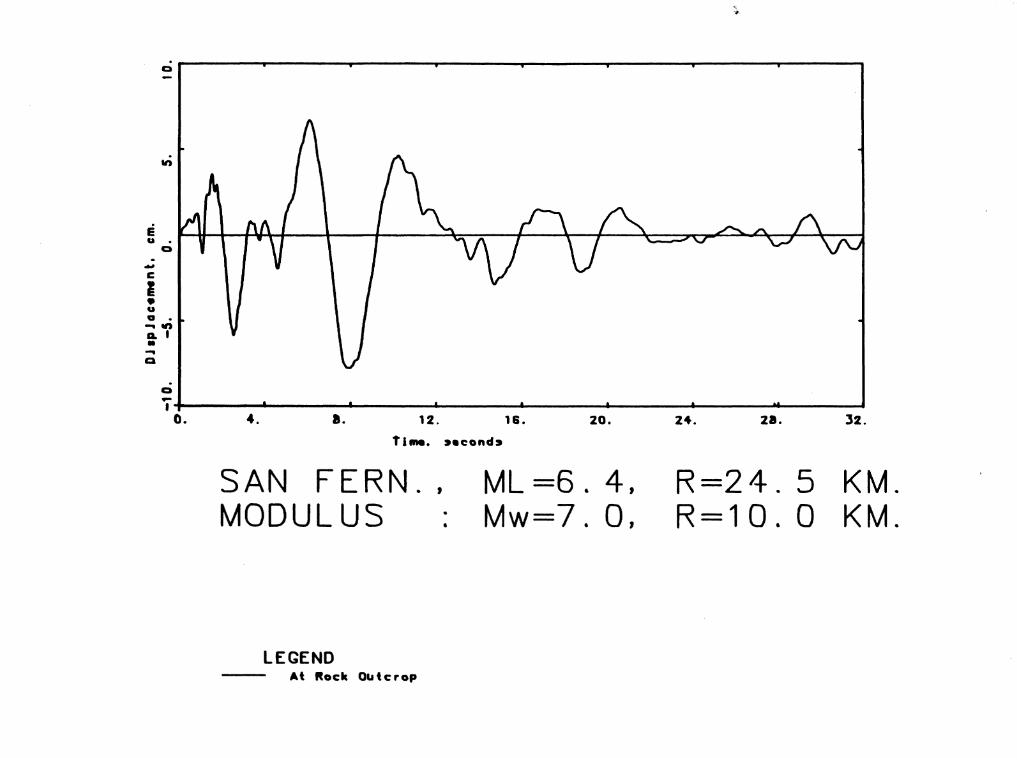
0 -
.,,
e u .
--C
I • u
Q
a . ... .,, A I • ... Cl
Q -
"#
,..,. ______ ..._ _______________ _... _____ _._ ____ __...._ ____ ...... ____ __,
o. 4. a. 12. 16. 20.
t line. :,•cond:1
SAN FERN. , MODULUS
LEGEND At Rock Olltcrop
ML=6. 4, Mw=7. 0,
24. 21. 32.
R=24. 5 KM. R=10. 0 KM.

. u • .. .......
" 0
.. 0 -
E .. u
•
10 -, 10 1
Frequency. Hertz
10 1 10 I
WES : WUS RESPONSE OUTCROP (Mw AT ROCK
LEGEND ---- At 20 a.
At Rock outcrop
7)

C)
-
II)
II
- 0 Ill.
0
C 0 ... ~
a r.. • II) .... • I u u
C
0 , ..... --.... --------------_.. ___________ __...._ ________________ _ o. 4. a. 12. 16. 20.
T lme. :t•c:ond:t
SAN FE RN. , MODULUS
ML=6.4, mb =7. 0,
24. 21, J2.
R=24. 5 KM. R=10. 0 KM.

c:i-------------..... --------------,,-------.... ------...--------------.
. u •
In
.,, N
• • ,a E u
.,.. - . ... .,, UN o I ... ;;
0 .,, 1-t---,t---_......._ __________ ..._ ____ __. _____ ..._ ______ .__ ____ ,.. ____ __.
Q. 4. a. 12. 18. 20.
T lme. :second,
SAN FERN., MODULUS
ML =6. 4, mb = 7. 0,
24. 28. 32.
R=24. 5 KM. R=10. 0 KM.

c:, -
In
E u .
. -C
I • u
c:,
a . - .,, A. I
" -Q
c:,
, ..... ------------------------------......i~------------------0. 4. a. 12. 18. 20.
Time. ,•cond,
SAN FERN., MODULUS
ML=6. 4, rnb = 7. 0,
24. 28. 32.
R=24. 5 KM. R=10. 0 KM.
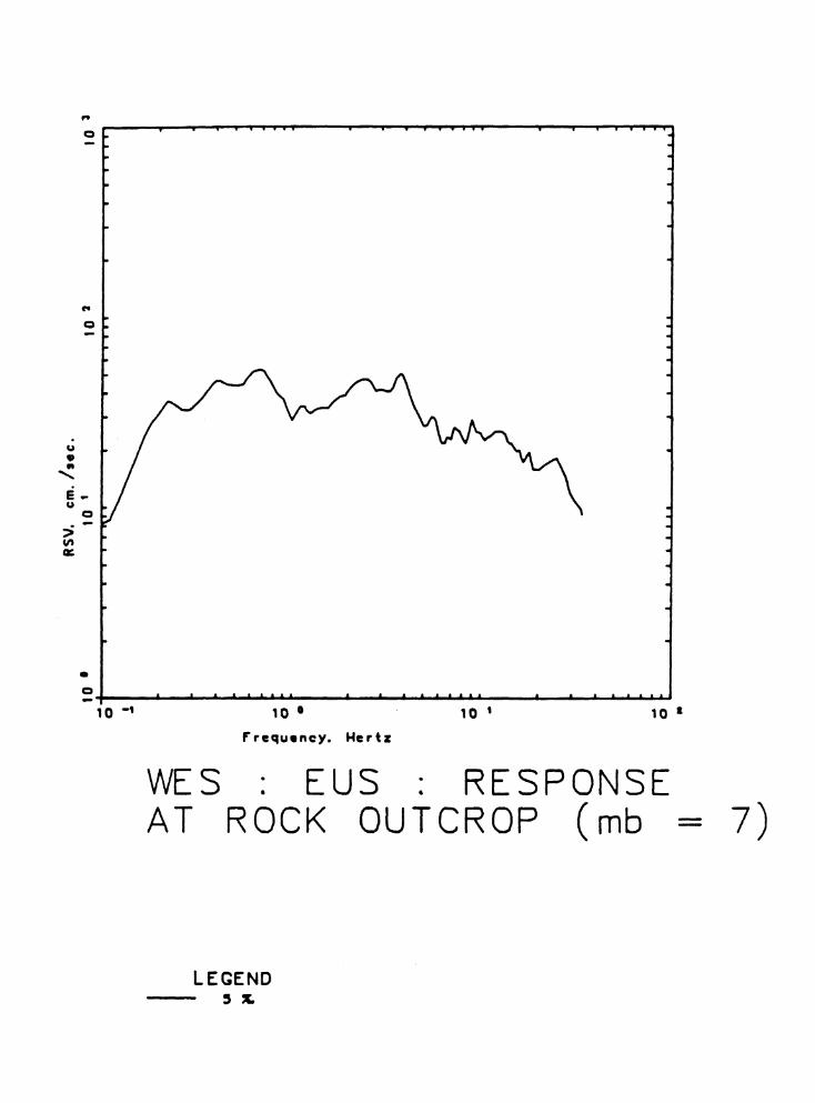
. u • ..
........
" Q -
" Q
E .. u
;;; en a::
Q -
• 10 -, 10 o t O 1 10 I
f' rcquency. Hertz
WES . EUS . RESPONSE AT ROCK OUTCROP (mb = 7)
LEGEND - 5""

0
-
"'
• - 0 .,. .
0
C 0 .... -a L. . .,, ..... • I u u <
0
-,+-_____ .._ _____ ..._ ____________ -&, ___________ __...._ _______ .__ ____ _
o. 4. a. 12. 16. 20.
Time. second:,
SAN FERN., MODULUS
LEGEND At 20 m.
ML=6. 4, Mw=7. 0,
24. 28. 32.
R=24. 5 KM. R=10. 0 KM.

. u •
Q .,,
.,, N
. . ,a e u
,. - . -.,, u ('I D I -J
Q .,, ,.,... _________________ _,_ __________ ..... _______________ _ o. 4. a. 12. 18. 20.
T!IMI. ••cond•
SAN FE RN. , MODULUS
LEGEND At 20 111.
•
ML=6.4, Mw=7. 0,
24. 28. 32.
R=24. 5 KM. R=10. 0 KM .
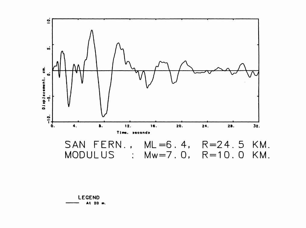
C) -
.,,
E u .
. -C
I • u
C)
a . ... .,, A. I • -Cl
C) -1+-------------------------------------------------0. 4. a. 12. 18. 20.
time. ,econd,
SAN FERN., MODULUS
LEGEND At 20 111.
ML =6. 4, Mw=7. 0,
24. 28. 32.
R=24. 5 KM. R=10. 0 KM.

Figure Set 9. Plots of response spectral scaling results.
A) Plot or response spectra. Open circles are from Boore (1983) and
represent regressions on WUS data for a moment magnitude 6 event at a
closest distance of 10 km. The upper solid line is initial RVT
response spectrum for a moment magnitude 6 event at a hypocentral
range of 10 km. Dashed-dotted line is the specified target response
spectrum scaled to 0.125 g. The dashed line is after two iterations
using the RVT calculated response spectra to scale the Brune spectra.
The solid lower line represents the final two iterations which employ
time domain calculations of the response spectra. Time histories are
calculated by adding an observed phase (from the time history library)
to the scaled Brune modulus.
B) Plot of Fourier spectral density after two iterations (dotted line)
and after four iterations (solid line). The first two iterations have
used the RVT calculated response spectra to scale the Brune spectra.
The final two iterations use time domain calculations to evaluated the response spectra.
C) Solid line shows effects of band-pass filters on response spectra.
The filters are fifth order Butterworth with corners at 4 seconds
(high-pass) and 23 Hz (low-pass). The filtering is done after the
last iteration. Remaining curves are the same as those in plot (A).
D) Resultant acceleration, velocity, and displacement time histories.
The response spectra for the acceleration time history is shown in
plot (C) solid line. Unnormalized peak acceleration is 0.116 g.

u • ..
.. C)
C)
' e. u
i C)
0
0
A '
-~------------------10 -, 10 o
frequency. Hertz
, 0 t 10 I
WES RESPONSE SPECTRA AT ROCK OUTCROP (Mw = 6)
LEGEND - · - De,ign Spectrum (~max - O. 12, g). , ,r dampihg

0 -
.,,
. u • • • ,a e u
,.. -.... u .,, o I ... ~
0 -
D
..... ______________________________________________ ,.. o. 4. a.
COYOTE MODULUS
12. 16. 20.
Time. ••cand•
. • ML=5. 9,
MW=6. 0,
24. 2a. l2.
R=18. 7 KM. R=10.0 KM.

. u • •
i C -
'i' C -
.!,. 'i'
"' < ... C -
.. I
10 -,
B
10 o
P'requ•n~y. Hertz
1 D ' 10 I
WES ·· FOURIER SPECTRA AT ROCK OUTCROP (Mw = 6)

•.. -·
E
N
' -
II •
-C
I • II a
0
-. -A. I • ... a
D
. "t+---------------------------------------------.... o. 4. a.
COYOTE MODULUS
~ ...... , __
12. 16. 20.
ti ... :t•cond:t
ML =5. 9, MW=6. 0,
24. 28. 32.
R=18. 7 KM. R=10. 0 KM.

"' C ___ ....,.....,,......__._ _____ .......... ___ _....._~
u • • '
-
C -
i. u
C
_; -"' CIC
.. I
C
C ' _..,._ _____ ......_. __________________ _
10 -, 10 •
P'requenll:ly. Mertz
10 1 10 I
WES . RESPONSE SPECTRA AT ROCK OUTCROP (Mw = 6)
LEGEND - • - Dealtn Speetrum (~ma• - O. 125 9). 5 ,r dat11Plt19

•
"" .
-•
- 0 •• 0
C 0 ... -0 ... ·-.... • I u u
C
""
D
i+-___________ ....., ________ __... ____________________ _
o. 4. a.
COYOTE MODULUS
12. 18. 20.
T 11•. aecond:s
ML =5. 9, MW=6. 0,
- ht e· ?#t+ I ~ ........ ....-. ........ _ .. _"'"-'"-' ... __ .
24. 21. 32.
R=18. 7 KM. R=10. 0 KM.

Figure Set 10. Plots of response spectra and acceleration time history
normalized to design value of 0.125 g.
A) solid line is the time domain calculated response spectra of the normalized acceleration time history. Remaining curves are the target response spectra (dashed-dotted) and the second iteration RVT response spectra (dotted).
B) Acceleration time history normalized to 0.125 g.

u 'II ..
........
.. 0
0
e. u
0
i
A
o+-__ _.._...___.__.__..~ ....... --__.-.......................... _._ ....... ....._ __ ....__...._...._...._...._......_.._. 10 _, 10 o 1 Q I 10 1
f' requency. Hertz
WES RESPONSE SPECTRA MA AT ROCK OUTCROP (Mw 6)
LEGEND Design Spectrum (Amox - O. 12:1 g). 5 "dompir,g Comp1,1ted "VT Spectrum (2 Iteration:,). 5 "dompir,g Computed SOP' Spectrum (4 Iteration:,). 5 "dompir,g

N
.. • Q a,
Q
C 0 ~ -a ... .. -..... • I u u <
C"t
B
1·1-____ ...., __________________ ..._ ____ ....,_ ________________ _
o. ... 8.
COYOTE MODULUS
12. 16. 20.
lime. :,ec:ond:,
ML =5. 9, MW=6. 0,
24. 28, 32.
R=18. 7 KM. R = 1 0 .' 1 0 KM.

Figure Set 11. Plots of results from a different scaling technique fitted
to the same target response spectra. Target and final response spectra
along with acceleration, velocity, and displacement time histories are
shown.

. • • ...: Ii
0 ..
• •• I; 0 L .-
T ! ... ________ _._.._._....._ ___ ...... ___ ._._._ _____ ..... _.__ ......... _ 10 ~
VAFB
LEGEND
• •
10 -t 10 • ,erletl. Hcentl•
DESIGN SPECTRA
De1ltn S,ectrua (Aalx • 0,115 9). 9 S tlaaplnt 9 & IASELINE CClltltECTED
10 1

0 • ------------T----,----~· = I
• ., J-• .... -
• 0 _J . w ., - u
u .,, <C . N -
0 0 w .
H 0 - • LL. ,, C: 0 H Cl • 0 • .,, . • 0 .... I - ~ ..
0 • • . .,,
en .,, LL • <C N
> 0 . 0
i· ' . o·o '·- i·-
••• •uor \DJ •r •ooy

I 0 . 0 N
~
1ft >-• .... - r-H
0 u • 0 1ft - _J
w 1ft > • N -
0 0 w .
H 0 - • I.J... ~ C 0 H u • 0 • 1ft
• • 0 .... I - ~ ... 0 • • . 1ft
CD 1ft I.J... . <{ N
> 0
• 0 ·oL ·s ·o ·;- ·oL-
·0••1·110 •iiroor•A

0 • -----------....-----. = :r:
• 1ft I-• ... ..
• 0 _J
• 0... 1ft .. (/) H
1ft 0 • N ..
0 0 w • H 0 ..
II l.J._ .,, C 0 H u • 0 II
1ft . • 0 ... I - 2 ... 0 • • • 1ft
Cl)
1ft LI-. <{ N
> 0 . 0
·i . ' ·o . ,- ·i-·110 '\U .. eODf di f Q

Figure Set 12. Plots of basis time histories which are used to supply phases to the Brune spectrums. Magnitude range and distance range criterion for matching to the Brune spectra are given in Table 4.

N C)
I -C) -•
.,,_
. • C)
Ill
-C 0 -. _, a .,, ._ I
• ... .. u u
C c -
•
11-----------------------------------------------------4 o. 4. a. 12. 16. 20, 24. 28, J2.
Time. :.•cond:.
OROVILLE AFTERSHOCK, 1975 ML= 4.0, R = 10.5 KM.

... Q I -C) -•
. .. Q
1:1111
-C D .... ..., a 111 L. I • .... • u u < c:i -11--t------------------------------------...._ _____ ....., _____ _,
o. 4. a. 12. 16. 20. 24. 28. 32.
Ti me. second,
OROVILLE AFTERSHOCK, 1975 ML= 4.9, R = 8.6 KM.

. ... Q I -Q .... •
. .. C,
Ill
C Q -. - . a 111 ~ I ..
I o.
"'
•• a. 12. 16. 20. 24. 2a. 32.
time. 2econd2
COYOTE LAKE, MAIN SHOCK, 1979 ML = 5. 9, R = 1 8. 7 KM.

"' 0 I -0 ... •
. .,, .
.. C)
Gt
C 0 .... ., a 111 ._ I
• .... • u u < C) -11-------+-----------------------------------------.. o. .... a. 12. 16. 20. 24. 28. 32.
T j me. ,econd:t
COYOTE LAKE, MAIN SHOCK, 1979 ML= 5. 9, R = 29. 4 KM.

..
N .
• - C Cl' •
Q
C 0 ... -a .. 9N .... • I u u
C .. 1+---------------------------------------------
0. 4. a. 12. 16. 20, 24. 2a. 32.
Time. >econd>
SAN FERNANDO MAIN SHOCK, 1971 ML= 6.4, R = 24.5 KM.

N en ""'
"' en . ~ ..
N
.. •
Z2 . H~ ...
N
<{
20 . •
0 N ~O
>- -tj-w . _J II co - " _J .,,
C
<{ et: 0 u • > " .
N . - • e ... - _J c.o ... <{ •
Hc.D ,0
et: w II Q_
... 2_J
H2 .
0 . 0 I ·~ ·o ·s- ·ol-
r.-0 l • 1, & 'UOflDJ•r•,,v