Embed Size (px)
Citation preview


STATEHOUSE DEMOCRACY


STATEHOUSE DEMOCRACYPublic opinion and policy in the American states
ROBERTS. ERIKSONUniversity of Houston
GERALD C.WRIGHTIndiana University
JOHN P. McIVERUniversity of Colorado
CAMBRIDGEUNIVERSITY PRESS

Published by the Press Syndicate of the University of CambridgeThe Pitt Building, Trumpington Street, Cambridge CB2 I RP
40 West 20th Street, New York, NY 10011-4211, USA10 Stamford Road, Oakleigh, Melbourne 3166, Australia
© Cambridge University Press 1993
First published 1993
Library of Congress Cataloging-in-Publication Data
Erikson, Robert S.Statehouse democracy : public opinion and policy in the American
states / Robert S. Erikson, Gerald C. Wright, John P. Mclver.
Includes bibliographical references and index.ISBN 0-521-41349-4. - ISBN 0-521-42405-4 (pbk.)
1. Public opinion - United States - States. 2. State governments -United States. I. Wright, Gerald C. II. Mclver, John P.
III. Title.HN90.P8E76 1993
3O3.3/8-dc2O 93-7076CIP
A catalog record for this book is available from the British Library.
ISBN 0-521-41349 4 hardbackISBN 0-521-42405 4 paperback
Transferred to digital printing 2002
Contents
Preface page vii
1. Democratic states ? 1
2. Measuring state partisanship and ideology 12
3. Accounting for state differences in opinion 47
4. Public opinion and policy in the American states 73
5. State parties and state opinion 96
6. Legislative elections and state policy 120
7. Political culture and policy representation 150
8. Partisanship, ideology, and state elections 177
9. State opinion over time 212
10. Conclusions: Democracy in the American states 244
References 254Index 265


Preface
In recent years, citizens of many nations have struggled to establishdemocratic institutions where none had existed before. As political scien-tists, we can ask what justifies this passion for "democracy?" Part of theanswer is easy: political freedom. Empirically as well as in theory, wheredemocratic institutions prosper, people are freer to speak and act withoutfear of arbitrary intrusion from government authority. But freedom fromgovernment intrusion is not the sole justification for democratic govern-ment. In theory, the democratic ideal of popular sovereignty means thatcollectively, citizens can actively shape what their governments do. Therelevant empirical question becomes whether, in practice, democratic in-stitutions allow public opinion to influence government policies verymuch. Modern political science is still working on the answer to thisimportant question.
This book addresses the question of democratic representation for oneset of democratic governments: those of the 50 separate states of theUnited States. The Constitution of the United States reserves many gov-ernment powers to the states. The policies that states enact are oftendescribed in terms of their ideological content as relatively liberal or rela-tively conservative. We use this ideological dimension to assess the corre-spondence between public opinion and policies across the states.
We began this project several years ago, from a sense that public opin-ion had been seriously neglected in the political science literature on statepolicymaking. As we assembled our statistical evidence, we found a pat-tern that was even stronger than our initial suspicions: State ideologicalpreferences appeared to dominate all other variables as a cause of theideological tilt of a state's policies. This result further stimulated us to seekan understanding of the mechanisms by which state electorates are able togenerate policy mixes that reflect their ideological tastes.
The states as political communities and as centers of policymaking havenot, in our opinion, received the research attention from the political
Vll

Preface
science community that they deserve. Political scientists' collective fas-cination with politics in Washington, D.C., has had the unfortunate con-sequence of neglecting the politics in the state capitals. At a time when thestates are increasingly the primary policy innovators and much of theattention in Washington is consumed with dealing with or avoiding thefederal budget deficit, the states should be an important focus for policyanalysis, as well as for testing more general theories of politics. We hopeour research will contribute to a renewal of the interest in comparativestate politics that flourished in the 1960s and 1970s.
This book, however, is about representation as much as it is about statepolitics. In this we see our work contributing to a revisionist view of thecitizen in politics. Earlier work focusing on individual opinion formationand decisionmaking through the lens of the sample survey found the typi-cal citizen sorely lacking in the requirements expected by the standards ofdemocratic theory. The role of the citizen in democratic governance, how-ever, is about the values and decisions of the mass public - of aggregates -not about individuals. Taking this macro-view of mass behavior and opin-ion yields a significantly more favorable view of the coherence and theimportance of public opinion in the United States.
To estimate the ideological preferences of the American states required amassive data collection effort. Our measures of state ideological prefer-ences are mostly based on the cumulative surveys of CBS News/New YorkTimes. Kathleen A. Frankovic of CBS News Elections and Surveys Unit,and Warren Mitofsky, then at CBS News and now head of Voter Researchand Surveys, deserve special thanks for collecting these data and for mak-ing the CBS/NYT polls accessible through the Interuniversity Consortiumfor Political and Social Research. John Benson of the Roper Center washelpful for guiding us through the Roper collection of Gallup polls. Thecontributions of several individuals were indispensable for the task ofmaking sense of what in effect was a cumulative survey of over 170,000individuals. We are grateful for the help and advice of a number of stu-dents, some of whom served as research assistants, others as interestedreaders and critical consumers of our data: Joseph Aistrup, Betinna Brick-ell, Robert Brown, Darren Davis, Thomas Carsey, Kisuk Cho, RobertJackson, Mohan Penubarti, David Romero, and Jeanne Schaaf. The datacollection would not have been possible without the financial support ofthe National Science Foundation (grants SES 83-10443, SES 83-10780,SES 86-09397 and SES 86-09562).
This project made use of far more data than simply the ideologicalpreferences of the states. For providing the wealth of state-level data thatmade our statistical analysis possible, we owe thanks to many among thecommunity of scholars who study the politics and the policies of the U.S.
vin

Preface
states. For allowing us to ransack their survey of state legislators, we owespecial thanks to Eric M. Uslaner and Ronald E. Weber; for allowing ussimilar privileges for their survey of national convention delegates, weowe special thanks to M. Kent Jennings and Warren E. Miller. For gener-ously providing us with his unpublished estimates of AFDC and Medicaidstate effort, we thank Russell Hanson.
Several colleagues have contributed by reading and critiquing our work.We especially thank Christine Barbour, Thomas R. Dye, James L. Gibson,Virginia H. Gray, Alexander Hicks, Robert Huckfeldt, Kathleen Knight,Jon Lorence, David L. Lowery, Donald Lutz, Michael B. MacKuen, BruceI. Oppenheimer, Benjamin Page, Lee Sigelman, James A. Stimson, RonaldE. Weber, Frederick M. Wirt, and Christopher Wlezien.
Some of our analysis draws on the material appearing in earlier articles:Wright, Erikson, and Mclver, "Measuring State Partisanship and Ideologywith Survey Data," Journal of Politics 47 (May 1985): 469-89; Erikson,Mclver, and Wright, "State Political Culture and Public Opinion, Ameri-can Political Science Review 81 (September 1987): 797-813; Wright,Erikson, and Mclver, "Public Opinion and Policy Liberalism in the Ameri-can States," American Journal of Political Science 31 (November 1987):980-1001; and Erikson, Wright, and Mclver, "Political Parties, PublicOpinion, and State Policy in the United States" American Political ScienceReview 83 (September 1989): 729-50. The research reported here is ap-preciably updated from these articles, incorporating measurement of stateideological preferences through 1988.
IX


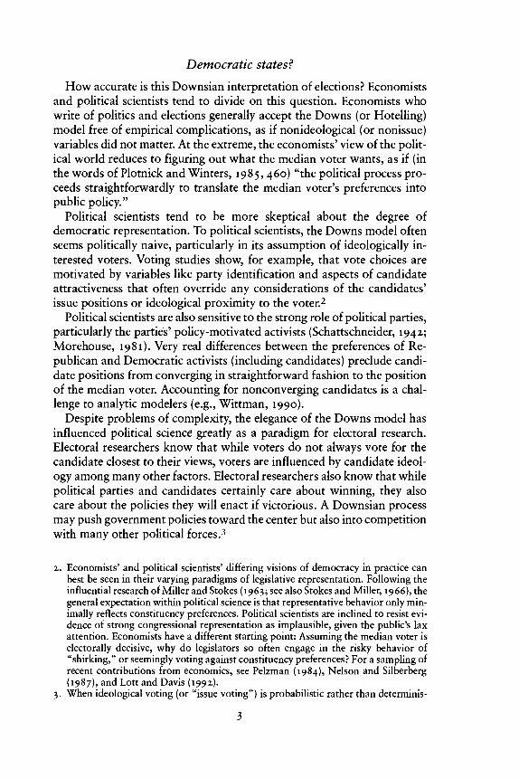
Democratic states?
Unless mass views have some place in the shaping of policy, all the talk aboutdemocracy is nonsense.
V.O.Key(i96i,7)
Popular control of public policy is a central tenet of democratic theory.Indeed, we often gauge the quality of democratic government by the re-sponsiveness of public policymakers to the preferences of the mass publicas well as by formal opportunities for, and the practice of, mass participa-tion in political life. The potential mechanisms of democratic popularcontrol can be stated briefly. In elections, citizens have the opportunity tochoose from leaders who offer differing futures for government action.Once elected, political leaders have incentives to be responsive to publicpreferences. Elected politicians who offer policies that prove unpopular orunpleasant in their consequences can be replaced at the next election byother politicians who offer something different.
Of course, this picture describes only the democratic ideal. A cynicwould describe the electoral process quite differently: Election campaignssell candidates in a manner that allows little intrusion by serious issues.Once in office, winning candidates often ignore whatever issue positionsthey had espoused. Voters, who seem to expect little from their politicians,pay little attention anyway.
The actual performance of any electoral democracy probably falls be-tween these extremes. Acknowledging the factors that impede effectivedemocratic representation, we can ask to what degree does public opinionmanage to influence government decisions? This is an empirical question,often noted as the central question of public opinion research (Key, 1961;Converse, 1975; Burstein, 1981; Kinder, 1983; Erikson, Luttbeg, and Te-din, 1991).
Ultimately, virtually all public opinion research bears on the question ofpopular control. The most directly related studies are those that examinethe statistical relationship between public opinion and public policies on

Statehouse democracy
specific issues, a task that is never easy (Weissberg, 1976; Monroe, 1979;Page and Shapiro, 1992). On balance, the somewhat ambiguous evidencesuggests that the government does "what the people want in those in-stances where the public cares enough about an issue to make its wishesknown" (Burstein, 1981, 295).
Almost all U.S. studies of the influence of public opinion focus on thenational level. However, the ideal place to investigate the relationshipbetween public opinion and public policy would seem to be the Americanstates. With fifty separate state publics and fifty sets of state policies, thestates provide an ideal laboratory for comparative research. Yet there hasbeen little research on the opinion-policy linkage at the state level. Thedecisive inhibiting factor has been the lack of good survey-based measuresof state-level public opinion.
This book attempts to fill this research gap. We develop new measuresof state-level opinion. They are the liberal-conservative ideological andthe partisan identifications of the state electorates. These new measuresare based on an aggregation of 13 years' worth of CBS News/New YorkTimes (CBS/NYT) national opinion surveys. The resulting data set hasrather large state samples, often exceeding the size of most national surveysamples. It provides the measures we need to explore the relationshipsbetween the ideological leanings of state publics and patterns of policies inthe states.
THEORY AND EXPECTATIONS
We approach our exploration of the opinion-policy connection in thestates guided by some conflicting expectations. One starting point is theelementary "democratic theory" of the sort developed by the economistAnthony Downs (1957) in his influential An Economic Theory ofDemocracy. Downs's model in turn draws on the work of an earlier econ-omist, Harold Hotelling (1929).1 In its basic form, the Downs modelassumes that voter preferences can be arrayed on a single ideological con-tinuum, from the political left to the political right, with citizens voting forthe candidate closest to their own position on this ideological spectrum.The basic Downs model also assumes competition between two politicalparties or candidates for majority support. These assumptions drive theoutcome: Parties and candidates converge toward the middle of the spec-trum, with the winner being the candidate closest to the median voter.Since the winning program converges toward voter preference at the mid-point of the ideological continuum, the policy result renders an accuraterepresentation of the composite position of the electorate as a whole.
1. Political scientists generally refer to the Downs model; economists often call it theHotelling model.
Democratic states?
How accurate is this Downsian interpretation of elections? Economistsand political scientists tend to divide on this question. Economists whowrite of politics and elections generally accept the Downs (or Hotelling)model free of empirical complications, as if nonideological (or nonissue)variables did not matter. At the extreme, the economists' view of the polit-ical world reduces to figuring out what the median voter wants, as if (inthe words of Plotnick and Winters, 1985, 460) "the political process pro-ceeds straightforwardly to translate the median voter's preferences intopublic policy."
Political scientists tend to be more skeptical about the degree ofdemocratic representation. To political scientists, the Downs model oftenseems politically naive, particularly in its assumption of ideologically in-terested voters. Voting studies show, for example, that vote choices aremotivated by variables like party identification and aspects of candidateattractiveness that often override any considerations of the candidates'issue positions or ideological proximity to the voter.2
Political scientists are also sensitive to the strong role of political parties,particularly the parties' policy-motivated activists (Schattschneider, 1942;Morehouse, 1981). Very real differences between the preferences of Re-publican and Democratic activists (including candidates) preclude candi-date positions from converging in straightforward fashion to the positionof the median voter. Accounting for nonconverging candidates is a chal-lenge to analytic modelers (e.g., Wittman, 1990).
Despite problems of complexity, the elegance of the Downs model hasinfluenced political science1 greatly as a paradigm for electoral research.Electoral researchers know that while voters do not always vote for thecandidate closest to their views, voters are influenced by candidate ideol-ogy among many other factors. Electoral researchers also know that whilepolitical parties and candidates certainly care about winning, they alsocare about the policies they will enact if victorious. A Downsian processmay push government policies toward the center but also into competitionwith many other political forces.3
2. Economists' and political scientists' differing visions of democracy in practice canbest be seen in their varying paradigms of legislative representation. Following theinfluential research of Miller and Stokes (1963; see also Stokes and Miller, 1966), thegeneral expectation within political science is that representative behavior only min-imally reflects constituency preferences. Political scientists are inclined to resist evi-dence of strong congressional representation as implausible, given the public's laxattention. Economists have a different starting point: Assuming the median voter iselectorally decisive, why do legislators so often engage in the risky behavior of"shirking," or seemingly voting against constituency preferences? For a sampling ofrecent contributions from economics, see Pelzman (1984), Nelson and Silberberg(1987), and Lott and Davis (1992).
3. When ideological voting (or "issue voting") is probabilistic rather than determinis-

Statehouse democracy
Thus, the correctness of the Downs model is a matter of degree. Forcandidates, appealing to the political center is important but not alwayscrucial. One can imagine an electoral system inhabited by voters so inat-tentive (or uninformed) regarding the ideological positions of candidatesthat elected politicians enact policies totally unburdened by the constraintof public opinion. One could also imagine the opposite, a system in whichthe electorate actually dictates the ideological tone of government policymaking. From the standpoint of democratic theory, this latter outcomemay be the more desirable. But we must ask, How much is required of theelectorate and of elected officials for public control of the direction ofgovernment policy to become reality?
Judging solely from what we now know about the political readiness ofthe typical voter, there might appear little hope for much policy represen-tation in any political arena, let alone the U.S. states. Thanks to the classicThe American Voter (Campbell, Converse, Miller, and Stokes, i960) andsubsequent research on electoral behavior, we have convincing evidencethat individual voters tend to be rather ignorant and indifferent aboutmatters of ideology and public policy. We should keep in mind, however,that collective outcomes, including election results, can be driven by arelatively small number of actors, not just those who are "typical." Econo-mists know this lesson well. When, for example, they forecast a responsein the national economy to a change in the prime interest rate, they natu-rally do not assume that the typical U.S. consumer is closely monitoringthe activities of the Federal Reserve Board. But they do assume that somesmall number of economic actors will watch and serve as the engine forgeneral economic change. We believe the political analogy here is quiteplausible. While we would not expect the typical U.S. voter to respond tothe politicians' everyday political posturing or specific roll call votes,some important individuals do pay attention, with consequences that canextend to the ballot box. Moreover, just as the Federal Reserve Board willanticipate the economic response to their actions, so too will politiciansgauge and anticipate the electoral response to their possible actions.
The question is, Where on the continuum of possibilities lies the truthabout democratic accountability? We know a lot about individual votersand some things about politicians, and not all of it is favorable for repre-sentative democracy. As U.S. government is currently practiced, are pol-icies guided by public preferences? A discerning reader of contemporarypolitical science might think not. This negative conclusion would seem to
tic, the exact median voter result does not necessarily hold. For instance, if issueproximity is represented as the difference in the squared differences between thevoter and each of two candidates (the common assumption), then the equilibriumresult is the mean voter preference. See Enelow and Hinich (1984) and Erikson andRomero (1990).

Democratic states?
be particularly compelling when the discussion centers not on matters ofcentral concern to the U.S. public, but rather on the arcane world of statepolitics. Sheltered from the public limelight and constrained by limitedresources on the one hand and federal requirements on the other, state-level policy making would seem to offer little leeway for innovation inresponse to public demands. Understandably, tracing the policy impact ofpublic opinion has received low priority in state politics research.
STATES AS LABORATORIES
The role of public opinion has been largely neglected in the study of statepolitics. One way of seeing this is to note the disjuncture in the importanceof public opinion in policy studies at the national versus the state levels. Innational studies, public opinion (and its expression through the electoralprocess) is frequently of central concern in explaining the processes ofpolicy development and change over time. Public opinion has a majorexplanatory role in historical studies of realignment (Burnham, 1970;Clubb, Flanigan, and Zingale, 1980), national policy change (Carminesand Stimson, 1989; Stimson, 1991; Page and Shapiro, 1992), and rollcalls and policy making in Congress (Miller and Stokes, 1963; Schwarz,Fenmore, and Volgy, 1980; Sinclair, 1982; Wright, 1986; Brady, 1988)and of course, voting in presidential elections particularly through thevery extensive use of National Elections Studies data. The pervasive atten-tion to the connections between public preferences and the actions ofgovernment on the part of scholars of national politics is not in the leastsurprising. Whether we try to make sense of the observed governmentbehavior or try to assess the democratic quality of policy making in theUnited States, we fully expect analysts to incorporate the public's prefer-ences about policy and judgments of politicians in their explanations ofpolitics.
In sharp contrast to this familiar attention to public opinion at thenational level, state policy studies have proceeded with only passing atten-tion to public opinion. A contributory reason surely is a prevailing schol-arly viewpoint that because state politics is beyond the attention of mostcitizens most of the time, there is little reason to expect state policies toreflect public preferences. In fact, more reasons are usually offered forwhy public opinion is irrelevant than for why it is influential. Jack M.Treadway's review of the state policy literature dismisses the contributionof public opinion this way:There is every reason to assume a lack of congruence between policy outputs andpolitical opinion. First, given the lack of public information and interest amongthe public, there will be many issues for which no public opinion exists. Second,even if opinions exist they must be conveyed to policymakers. Since few citizensregularly contact their elected officials, it is quite possible that opinions will not be
5

Statehouse democracytransmitted to the policymakers. . . . Third, even if policymakers hear from thepublic they may choose to ignore what they hear. Finally, because the public isgenerally uninformed about the policy attitudes and activities of their elected lead-ers, they may not be aware of how accurately their opinions are being reflected bypolicymakers. A lack of congruence between public opinion and public policycould be perpetuated by public ignorance that such a situation exits. It seems likelythat would be more of a problem at the state level. (Treadway, 1985, 47)
Treadway's articulation, though unusually explicit, is consistent with thegenerally implicit assumptions of much of the state policy literature. Inpractice, explanations of patterns of policy in the states have incorporatedan impressive range of variables, but only sporadically have public prefer-ences been among them. From reading the state policy literature, onemight conclude that policies generate mysteriously from a variety of state-level variables ranging from state affluence to the professionalism of thelegislature. The idea that policy choices might be driven by electoralpolitics - so common in the national-level literature - is seldom articulatedin literature on state policy.
This neglect of the potential opinion-policy connection in the statepolitics literature represents a missed opportunity. At the national level,effects of public opinion are often difficult to ascertain because the rate ofopinion change on most issues is slow and often entangled with the flowof events and policy change itself (Page and Shapiro, 1992). The states, bycontrast, offer real-world laboratories for the comparative study of allsorts of political processes (Jewell, 1982). Since the individual states en-compass groups of citizens of widely varying political attitudes and val-ues, scholars can use this variation to assess the responsiveness of statepolicies to citizen policy preferences. Additionally, the states offer an op-portunity for the analysis of the impact of political structures on theopinion-policy representional process that cannot be done at the nationallevel, where but a single set of unvarying institutions prohibits effectiveassessment of their effects on representation.
Comparative analysis of the U.S. states, therefore, offers great potentialfor research on public opinion-public policy linkages. However, this po-tential has not been exploited. The reasons, we have suggested, appear tobe twofold: a lack of adequate data on the preferences of state electoratesand problems of conceptualization concerning the policy processes instate studies.
Measuring state opinion
The central reason for ignoring public opinion in the states is a practicalproblem of inadequate data on state opinion. The explanation for this gap

Democratic states?
in our data collection was identified by Richard Hofferbert in his sum-mary of the state policy field:
A glance at the literature makes clear the difficulty of studying all the intricacies ofindividual citizens' political participation. If such "micro" data are to be the basisof comparative analysis at the aggregate (for example state) level, the problems ofdata collection alone (not to mention conceptual difficulties) are nearly astronomi-cal. . . . To make equally accurate estimates about the residents of all fifty states,one would have to interview fifty times as many people as are included in thenational sample. Neither the resources nor the motivation to do a sample survey of75,000 people has yet risen to the task. (1972, 22-23)
Still, some scholars have seen the relationship between public opinionand state policy as sufficiently important to risk assessing the role ofpublic opinion indirectly. Not surprisingly, surrogate measures of stateopinion have their drawbacks; each rests on tenuous assumptions regard-ing the linkage between the intended attitudes and the measurable vari-ables. We consider some examples.
One common substitute for direct measurement is the "simulation" ofstate opinion from the demographic characteristics of the state residents(Pool, Abelson, and Popkin, 1965; Weber and Shaffer, 1972; Weber et al.,1972). For instance, Weber and his associates (Weber and Shaffer, 1972;Weber et al., 1972) "simulated" state opinion on a variety of issues. Usinga two-step process, they first used national opinion surveys to establishthe opinions that were typical for groups of citizens defined by their com-binations of social and economic characteristics. The simulation then con-sists of constructing a state opinion index that represents an average of thegroups' opinions weighted by the sizes of the groups in the states'populations.
Weber et al. report strong relationships between simulated opinion andpolicy on two of the five issues they examined. Unfortunately the simula-tion technique suffers from two important problems. One problem is that"simulation" taps only the demographic sources of opinion and not thosedue to the state's political culture or the state's particular history. Second,these demographic sources of opinion may reflect the causal impact of thesocioeconomic indicators themselves rather than the impact of publicopinion (Seidman, 1975).
We can also mention other efforts. In a simpler procedure, Nice (1983)inferred state ideological preferences from the state two-party vote in theideological Nixon-McGovern presidential election of 1972. Nice foundstrong and significant relationships between the McGovern vote and sev-eral indicators of state policy, most of which survived controls for stan-dard demographic variables. Although Nice produced some of thestrongest evidence of policy responding to public opinion, doubters may

Statehouse democracy
question whether the predictive power of presidential voting is due toideology or something else.4
Finally, the dilemma of how to measure state opinion is made evidentfrom Plotnick and Winters's (1985) analysis of state welfare policy. Need-ing measures of "voter preferences for redistribution," Plotnick and Win-ters chose per capita United Way contributions and charitable deductionson federal income tax returns as a percentage of adjusted gross income.These measures performed miserably in an otherwise satisfactory causalmodel explaining state welfare guarantees. As Plotnick and Winters ex-plain, "Although this first effort at measuring voter sentiments at the statelevel and identifying its effects on policy is disappointing, it demonstratesthe need for better measurement of this theoretically important variable"(1985,469).
Armed only with weak, indirect, or dubious measures of state opinion,analysts who dare estimate the opinion-policy connection cannot easilybe sure of their results. A poorer than expected correlation can be due topoor measurement. A strong correlation, on the other hand, can be chal-lenged on the grounds that the surrogate measure of public opinion actu-ally measures something else.
State socioeconomic variables
In lieu of the generally unmeasurable preferences of state electorates, statepolicy researchers have focused on variables that they could actually mea-sure. The central preoccupation of the state policy literature has been anongoing contest between "political" and "socioeconomic" variables ascompeting explanations of state policies. Socioeconomic (or "environ-mental") variables, by almost all accounts, are the winners of this contest.Such variables as state wealth, urbanism, and education appear to be thebest predictors of state policy. These predictors work at the expense ofcertain political variables, such as voter participation, party competition,and the quality of legislative apportionment. With socioeconomic vari-ables controlled, these political variables do not predict policy liberalismin the manner once hypothesized (Dawson and Robinson, 1963; Dye,1966; Hofferbert, 1966, 1974).
Yet considerable uncertainty exists regarding what the socioeconomicindicators actually measure. An early and influential view is Dye's "eco-nomic development" interpretation (1966, 1979). Dye posited that thesocioeconomic measures reflect the stages of economic developmentthrough which states evolve. As states become more developed, they also
4. The 1972 presidential vote has often been used as a surrogate for the ideologicalpreferences of congressional districts. See, e.g., Schwarz and Fenmore (1977) andErikson and Wright (1980).

Democratic states?
adapt a predictable set of policies. But while the state's economic base andsocial needs matter, state politics does not.
Dye's analysis was widely interpreted to mean that the workings of thedemocratic political process are largely irrelevant to understanding statepolicy. But this verdict now seems premature. For instance, it may havebeen naive to assume that if "political" variables like party competition,voter turnout, and proper apportionment enhance popular control, theywould always do so by stimulating liberal or pro-"have-not" policies. Abetter assumption would have been that these variables enhance thedemocratic process by facilitating the translation of the majority view-point into law, whether it is liberal or conservative (Godwin and Shepard,1976; Uslaner, 1978; Plotnick and Winters, 1985).
More important for our purposes is the question of whether the predic-tive power of the socioeconomic variables reflects something more thanthe deterministic force of economic development. On this, the early litera-ture expressed a certain ambivalence.5 Some scholars have expressed theview that socioeconomic variables reflect the input of political "demands"(Jacob and Lipsky, 1968; Godwin and Shepard, 1976; Sigelman andSmith, 1980; Hayes and Stonecash, 1981). The difference between seeingsocioeconomic variables as reflecting economic development and seeingthem reflecting political demands may seem little more than a matter ofsemantics. But if we go one step further and substitute "public opinion"for political "demands," we can begin to see the importance of this dis-tinction. We may then speculate that the predictive power of socioeco-nomic variables is due to the correlation of these variables with theunobserved variable of public opinion, which is actually a major determi-nant of state policy. Dye (1990, chap. 2) offers an interesting exposition ofthis new interpretation.
We have, then, two distinct views of what socioeconomic variablesstand for. Seen as nonpolitical indicators of economic development, socio-economic variables cause policy through some unspecified, but nonpoliti-cal process. Elections, legislators, interest groups, and citizens play outtheir roles in a sideshow devoid of policy consequences. The implications
5. Consider a typical example from the literature of the 1960s and 1970s. From con-ducting a factor analysis on state socioeconomic characteristics, Hofferbert (1968)identified the two dominant dimensions as "industrialization" and "cultural enrich-ment." Labeling a factor as "cultural enrichment" would seem to imply that it tapscitizens' values and preferences rather than economic determinism. However, label-ing a socioeconomic composite as "opinion" or "values" requires a strong act offaith. It is difficult to give an unambiguous attitudinal interpretation to factors thatare made up of indicators of wealth, ethnicity, and education. This uncertainty aboutwhat is measured is reflected in Hofferbert's subsequent analysis in which the cultur-al enrichment label is converted to an equally apt but perhaps safer choice of "afflu-ence" (Sharkansky and Hofferbert, 1969; Hofferbert, 1974).

Statehouse democracy
for meaningful democratic governance could hardly be more perverse. Butwhen the same socioeconomic indicators are seen as measures of publicopinion, the findings that socioeconomic variables "cause" policy yields apositive message about democracy in the U.S. states. High correlationsbetween environmental measures and policy show that public demand isusually satisfied; state politics "works." In fact, in this view, low correla-tions between socioeconomic measures and policy would be evidence thatstate political institutions fail to translate public preferences into policy.
In summary, the role of state public opinion has not fared well in thecomparative study of state policy. Much of the literature has emphasizedthe importance of socioeconomic variables. These variables are easilyquantifiable and predictably potent, but their theoretical meaning con-tinues to be unclear. Variables that are not readily measurable, like statepublic opinion, have received lesser recognition. Studies that do give statepublic opinion full attention are handicapped by severe problems ofmeasurement.
THE PRESENT STUDY
Our thesis is that public opinion is of major importance for the determina-tion of state policy. We will show that in terms of ideological direction,state policies tend to reflect the ideological sentiment of the state elector-ates. Moreover, we will show that party elites and two-party electoralpolitics, as these interact in the American states, are crucial elements in thelinkage process. The progression of our argument can be seen in the fol-lowing summary of the chapters to come.
Chapter 2 introduces our state opinion data. From pooling CBSNews/New/ York Times surveys from 1976 to 1988, we obtain measures ofstate ideological identification and state partisan identification. Chapter 2presents this data and describes the reliability and stability of the newmeasures of state opinion. Chapter 3 asks the question of where thesedifferences in ideology and partisanship among the states come from.While some of the state-to-state differences in ideology and partisanshipare attributable to differences in demography, we also find that state ofresidence has a large impact on citizens' liberalism-conservatism and par-tisanship even after state demographics are taken into proper account.States are active and meaningful political communities whose electorateshave distinctive preferences; the states are not just collections of atomisticindividuals whose opinions automatically flow from their personal socio-economic characteristics.
Chapter 4 introduces our composite measure of state policy liberalism.This chapter shows that the ideological direction of state policy largelyfollows from the state citizens' mean ideological preference. Policy and
10

Democratic states?
opinion, in other words, are highly correlated. As part of this demonstra-tion, Chapter 4 shows that the well-known correlations between socio-economic variables and policy liberalism (previously discussed) actuallyreflect the effect of opinion on policy. To the extent that socioeconomicvariables predict policy, they do so because they correlate with stateopinion.
Chapter 5 shows how the ideological preferences of Democratic andRepublican elites reflect the pull of their own "extreme" ideologies in onedirection and the push of the electorate's ideological moderation in theother direction.
Chapter 6 presents our general model of the policy process in the states.It shows how state electorates control the ideological tone of state policyby rewarding the state parties closest to their own ideological views, andhow party control does have policy effects, albeit in ways that are morecomplex than is commonly thought.
Chapter 7 examines the theory of state political culture developed bypolitical scientist Daniel Elazar. We find rather strong evidence that Elaz-ar's typology of state cultures distinguishes among states in terms of theirrepresentational processes.
Chapter 8 renews the focus on state elections by using Election Day exitpoll data to assess the different ways states vote for president, U.S. sena-tor, and governor. Here we find important interoffice differences in somepatterns of electoral behavior. Our analysis includes factors from both themicro- and macrolevels to demonstrate an important relationship be-tween state partisanship and state ideology that is completely missed ateither level alone.
Chapter 9 examines the state representation process - from the 1930s tothe present - by utilizing Gallup poll questions to create aggregate mea-sures of state ideology and state partisanship.
Chapter 10 summarizes our findings in accounting for how apatheticand generally poorly informed state electorates are able to achieve re-markably high levels of popular control over a broad range of state pol-icies. The process is anything but automatic; representation requireselectoral competition and motivated party activists to achieve statehousedemocracy.
1 1

Measuring state partisanship and ideology
When analysts classify the citizens of the various American states in termsof their political differences and similarities, the standards most oftenimposed are in terms of partisanship and ideology. One can generallyclassify a state's partisan tendencies with some assurance, since we canmake inferences from state voting patterns and, in some instances, partyregistration. Classifying electorates on the basis of ideology is riskier forthe reason that available indicators of ideology are at best indirect. Politi-cally knowledgeable observers do commonly attribute liberal or conserva-tive tendencies to state electorates. Among the factors that enter into theseimpressionistic judgments are the states' electoral affinities for liberal andconservative candidates, the ideological proclivities of their congressionaldelegations, and the general imprints of their unique political histories.Still, it is far from certain that state electorates' ideological reputations aredeserved. It may be an unwarranted leap of democratic faith to attributeideological motive to ideological consequences.
For our investigation of the public opinion-policy connection in theU.S. states, the most crucial challenge is the measurement of state-levelpublic opinion. This chapter presents our measures of state-level ideologi-cal identification and partisan identification, from CBS/NYT polls. Ouroverall strategy is straightforward. We simply aggregate by state the re-sponses to the 122 national CBS/NYT telephone polls for the period1976-88. These polls are conducted on a continuous basis, maintain thesame questions for party identification and ideology throughout the timeperiod, and use a sampling design that serves our purposes very well.
Actually, CBS/NYT conducts three different types of surveys: generalsurveys representative of the full adult population, surveys of only regis-tered voters (interviewees are screened for registration at the beginning ofthe interview), and Election Day polls of voters as they leave the votingbooths. The first two are telephone interviews and employ identical sam-pling designs. The exit polls, which are quite different, include fewer states
12

Measuring state partisanship and ideology
and are not used for our estimates of state partisanship and ideology. (Wedo, however, make occasional use of exit poll data apart from our mainanalysis.)
CBS NEWS/NEW YORK TIMES POLLS
For our state estimates, we combined 122 CBS/NYT surveys. Of these,113 are general population surveys, and 9 are registered voter polls. Re-spondents were asked about their party identification in all 122 surveys. In118 surveys, they were asked their ideological identification. Our file con-tains 167,460 respondents from 48 states plus the District of Columbia.Of these, 157,393 revealed their party identifications by telling CBS/NYTinterviewers they were a Democrat, Republican, or Independent. And141,798 gave usable ideological identifications as "liberals," "conserva-tives," or "moderates."
The number of respondents per state is built up through aggregation bystate and over time. The state sample sizes vary directly as a function ofstate population - the correlation between our state sample size and state1980 population is .99. Since state populations vary substantially, so dothe sizes of our state samples. While the state samples contain about 3,500respondents on the average (certainly an adequate number), the variabilityis such that some states have more respondents than necessary and othersnot enough. At one extreme, over 14,000 Californians and over 11,000New Yorkers were interviewed over the 1976-88 time period. At theother extreme, fewer than 600 respondents were interviewed in the leastpopulous states of Wyoming, Delaware, South Dakota, North Dakota,and Nevada. Our smallest working "N" is the set of only 292 self-proclaimed liberals, moderates, or conservatives in the state of Wyoming.
An even greater concern than adequate Ns for the state samples is thepotential problem of unrepresentative samples at the state level. Forperiodic national in-person surveys conducted for the National ElectionStudies, for annual General Social Surveys, or for commercial polls likethe Gallup poll, the pooling of respondents by states would produce mis-leadingly inefficient estimates. Typically, all of a state's respondents in anational survey will reside in only one or two counties (and a few neigh-borhoods within these counties). Moreover, for understandable reasons ofconvenience, survey organizations tend to maintain the same counties intheir sampling frames for up to a decade or more. Thus, even with a largepooled N, a state's sample may be representative of only the small numberof counties within the sampling frame.
Fortunately, the CBS/NYT surveys use a random-digit dialing designthat largely overcomes this problem (Waksberg, 1978). The design hasvery small clusters compared to in-person surveys, and these are generally
13

Statehouse democracy
more widely dispersed geographically than interviews within the blockclusters of personal interview samples. Rather than the 80 or so primarysampling units (or PSUs) typical of national in-person surveys, the CBS/NYT polls each have about 400 PSUs. This provides a wider dispersion ofrespondents and hence more efficient estimates of state opinion.
Technically, the CBS/NYT survey PSUs are defined by an area code andthe first five digits of a valid residential exchange (e.g., [714] 527-09XX).Interviews are then taken from a sampling frame made up of hundreds ofthese sets of 100 possible numbers. Generally three interviews are takenfrom each exchange for a given survey. CBS/NYT surveys draw new sam-pling frames about once every two years. Aggregating over these differentsampling frames increases the number of communities and areas fromwhich respondents in these surveys, and hence from each state, have beenselected. Thus, there is good reason to expect that these data, taken to-gether, constitute valid samples of the individual states for the time period.
One final point deserves mention. For our construction of state mea-sures of partisanship and ideology, we include CBS/NYT survey respon-dents in the relatively small number of "registered voter only" surveys. Ina related decision, we count the "raw" numbers of respondents withoutemploying the weights suggested by CBS/NYT surveys for improving therepresentativeness of the samples. The alternative would be to weightrespondents, but also jettison the precious respondents from "registeredonly" samples. (For further discussion of the technical considerations, seeWright, Erikson, and Mclver, 1985.) Strictly speaking, our state estimatesare not strictly representative of state adult populations, but rather tiltslightly toward what might be called the "active electorate."
Presenting state partisanship and ideology
In the CBS/NYT surveys, respondents' partisanship is measured by theiranswers to the question, "Generally speaking, do you consider yourself aRepublican, a Democrat, an Independent, or what?" Ideology is assessedby asking the questions: "How would you describe your views on mostpolitical matters? Generally, do you think of yourself as liberal, moderate,or conservative?" These questions are similar to the standard AmericanNational Election Study questions on partisan and ideologicalidentification.
Tables 2.1 and 2.2 present the results of our state aggregations for the48 contiguous states plus the District of Columbia. (No estimates areavailable for Alaska and Hawaii.) Shown are the percentages for each self-identified partisan and ideological category, as well as the number of us-able respondents on which they are based. State positions on the twotrichotomized measures are summarized as mean positions. These means
14

Table 2.1. Partisan identification in the United States, 1976-88
State
AlabamaArizonaArkansasCaliforniaColoradoConnecticutDelawareDistrict of ColumbiaFloridaGeorgiaIdahoIllinoisIndianaIowaKansasKentuckyLouisianaMaineMarylandMassachusettsMichiganMinnesotaMississippiMissouriMontanaNebraskaNevadaNew HampshireNew JerseyNew MexicoNew YorkNorth CarolinaNorth DakotaOhioOklahomaOregonPennsylvaniaRhode IslandSouth CarolinaSouth DakotaTennesseeTexasUtahVermontVirginiaWashingtonWest VirginiaWisconsinWyoming
Republican
23.4%34.720.333.332.624.528.718.832.721.037.328.732.932.438.325.520.027.024.215.829.827.327.026.827.440.231.831.827.526.329.727.636.231.029.931.234.815.527.538.426.526.141.928.629.424.028.627.134.5
Independent
32.2%29.932.827.338.843.240.628.827.931.039.036.536.038.132.724.824.743.529.450.038.335.829.238.640.428.931.246.339.931.732.625.836.633.619.230.226.856.433.221.334.234.533.548.037.944.122.738.735.1
Democrat
44.4%35.446.839.428.632.330.752.439.348.023.834.831.229.629.049.855.329.546.434.231.936.843.834.632.230.937.021.832.642.037.746.627.335.450.838.638.428.239.240.339.339.424.523.432.731.948.734.230.3
Mean
21.10.6
26.56.2
-4.07.82.0
33.66.6
27.0-13.5
6.1-1.7-2.8-9.324.335.3
2.422.218.32.19.5
16.77.84.7
-9.35.1
-10.05.1
15.78.0
19.0-8.94.4
20.97.43.7
12.711.72.0
12.913.4
-17.4-5.13.37.8
20.17.1
-4.2
N
2,4191,7671,727
14,7731,8632,269
443565
7,4663,814
7247,0963,9642,2302,0372,4582,405
1112,9964,1586,8063,1811,4163,583
5941,252
487760
5,252843
11,5993,885
4957,7782,1152,0638,710
6142,304
7173,1499,696
966448
4,2453,1791,5593,413
333

Table 2.2. Ideological identification in the United States, 1976-88
State
AlabamaArizonaArkansasCaliforniaColoradoConnecticutDelawareDistrict of ColumbiaFloridaGeorgiaIdahoIllinoisIndianaIowaKansasKentuckyLouisianaMaineMarylandMassachusettsMichiganMinnesotaMississippiMissouriMontanaNebraskaNevadaNew HampshireNew JerseyNew MexicoNew YorkNorth CarolinaNorth DakotaOhioOklahomaOregonPennsylvaniaRhode IslandSouth CarolinaSouth DakotaTennesseeTexasUtahVermontVirginiaWashingtonWest VirginiaWisconsinWyoming
Conservative
40.5%37.436.831.631.329.432.024.637.136.642.532.536.033.036.533.740.036.130.428.231.633.241.234.434.337.529.634.230.136.230.437.840.532.442.032.833.029.039.838.436.640.644.134.837.029.232.232.639.7
Moderate
42.0%43.444.643.146.145.648.244.442.944.642.945.144.747.542.945.843.042.644.844.545.646.543.046.742.543.741.044.543.243.642.445.145.645.243.442.344.544.141.847.243.342.039.741.743.947.544.845.438.4
Liberal
17.5%19.218.625.422.625.019.831.020.018.814.622.419.319.520.620.517.021.324.827.322.820.415.818.923.218.829.421.326.720.227.317.113.922.314.724.922.426.918.414.420.117.416.123.519.123.323.022.121.9
Mean
-23.1-18.2-18.3
-6.2-8.6-4.4
-12.26.3
-17.1-17.7-27.9-10.1-16.7-13.5-15.9-13.2-23.0-14.7
-5.7-0.8-8.8
-12.8-25.4-15.5-11.1-18.7
-0.2-12.8
-3.4-16.0-3.1
-20.7-26.6-10.1-27.3
-7.9-10.6-2.1
-21.4-24.1-16.6-23.2-28.0-11.4-17.9
-5.9-9.2
-10.5-17.8
N
2,1421,5781,528
13,3691,7242,095
409504
6,7353,443
6666,4563,5101,9801,8102,1032,119
6852,7233,7046,1352,9421,2233,167
5511,128
446685
4,833746
10,6193,326
4477,0131,8661,8907,783
5622,128
6272,7648,745
868405
3,9482,9151,3483,113
292

Measuring state partisanship and ideology
are calculated by assigning a score of -100 to each Republican or conser-vative, a score of o to each Independent and moderate, and a score of+100to each Democrat or liberal and then calculating the mean in the standardway. Measured in this metric, the mean has an easy interpretation as therelative percentage point difference between the Democrats and Republi-cans or between liberals and conservatives.
The reader may wonder why we score liberals and Democrats as posi-tive and conservatives and Republicans as negative. We do so for onepractical reason. Later in this volume, we relate state opinion to statepolicy. State policy variables are generally scored so that "high" scores arein the liberal direction (money spent, regulations enacted, etc.). It makesgood sense to score the independent variable and the dependent variablewith the same polarity.
Consider first the estimates of state partisanship. Based on our meanpartisanship scores, the map in Figure 2.1 portrays the partisan landscapeof the United States. At the national level, the Democratic Party has out-numbered the Republican Party in terms of party identifiers, even duringthe Reagan era. So, naturally, we must find a Democratic edge for thestates as a whole. Indeed, Republican Party identifiers outnumberDemocratic identifiers in only 11 of the 48 sampled states. These Republi-can states are generally found scattered throughout the rural West andMidwest. At the other end of the partisan spectrum, the most Democraticstates cluster in the South and Border regions.
Consider next the estimates of state ideology. Based on our mean ideol-ogy scores, the map in Figure 2.2 portrays the ideological landscape of theUnited States. Just as Democrats have dominated the Republicans interms of partisan identification, conservatives have numerically domi-nated liberals in terms of ideological identification. But whereas somestates tilt in the Republican direction, every single state in the union (withthe possible exception of Alaska and Hawaii for whom we have no data)contains more conservative identifiers than liberal identifiers. The onlypolitical entity for which we have data that is more liberal than conserva-tive is not a state. The District of Columbia, also included in the CBS/NYTpolling, displays a slight liberal tilt.
The ideological map presented in Figure 2.2 shows the geography ofideology to be quite different from partisan geography. The most conser-vative states are found in the Deep South and in the rural West. The mostliberal states cluster along the Pacific rim and in the Northeast.
Figure 2.3 presents the data in still another way, as a scatterplot be-tween state ideology and state partisanship. In general, there is no discern-ible statistical relationship between state ideology and state partisanship.Indeed, the correlation coefficient is a mere .08. Only if we separate outthe southern states does even a mild (r - .48) statistical relationship
17

Statehouse democracy
I I Republican
[H7I O-A.9% Dem
llijjjl 5-9.9% Dem
i l l 10% Dem & More
Figure 2.1 Map of State Partisanship (Percent Democratic minus PercentRepublican).
I—I Most ConservativeI—I (Less Than-20%)
[ 7 ] (-20 to -15.1%)
H U (-15 to-10.1%)
mm Most Liberali i l i l (-10% and More)
Figure 2.2 Map of State Ideology (Percent Liberal minus PercentConservative).
18

Measuring state partisanship and ideology
10
0 "
- 1 0 "
- 2 0 "
- 3 0 "
- 4 0 "
NHKSNE
UT ID N D
NJMCAW
VT n S r "IA D E
ME M(
WY^AZVA F L
SD
y Rl
k\IVIN
scTX
MA
MD
WV
KY
NCAL LA
MSOK
I
-20i
-10 10I
20 30 40
Mean Partisanship
(Democratic minus Republican)
Figure 2.3 State Ideology and State Partisanship
emerge between the two indicators of mass political preference in thestates. Figure 2.3 also shows clearly that the range of states on the meanpartisanship index is considerably greater than the range of ideology. Asstatistical indicators, the standard deviations are 11.43 f° r t n e former and7.30 for the latter.1
Nevada: A statistical outlier
In general, the estimates of state partisanship and ideology are quite rea-sonable. Even those estimates from states with relatively small samplesgenerally possess a certain face validity. One exception, however, is theideological score for Nevada. Based on the ideological preferences of 446respondents, Nevada scores as the most liberal of all states, with almost aplurality preferring the liberal label. We believe that this score for Nevada
1. The District of Columbia and Nevada are omitted from the calculations for thesestatistical estimates of standard deviations and correlations. Except where otherwisenoted, the statistics reported in this volume are based on calculations with theDistrict of Columbia and Nevada removed. Regarding Nevada, see the discussion inthe following section.

Statehouse democracy
is so implausible that we substitute a more conservative coloring for thestate in our map of state ideology.
Although Nevada certainly enjoys a reputation for what might be con-sidered as social liberalism (legalized gambling and prostitution), there islittle reason to believe it to be the hotbed of political liberalism that ourpooled state survey would suggest. As judged by its presidential voting,the behavior of its congressional representatives, and the presence of asignificant Mormon population, the signs suggest Nevada is quite politi-cally conservative, like many of its western neighbors.
Important side evidence from CBS/NYT exit polls for Nevada clinchesthe validity of our concern about Nevada's ideology. Estimates of Nevadaideology based on over 2,000 CBS/NYT exit poll responses place Nevadaclearly among the most conservative states. Among the 42 states withavailable CBS/NYT exit poll estimates of ideology, Nevada ranks 11th inconservatism! Our conclusion is that the observed ideology score for Ne-vada is a sampling fluke - a score that is substantively implausible but stillwithin the range of remote statistical possibility, given the state's smallsample size.2
This Nevada estimate presents a minor annoyance with no clearly idealsolution. We could ignore the problem and use the Nevada estimate in ouranalysis. Our results would be slightly less crisp than otherwise, due toour rigid inclusion of a clearly incorrect estimate. Alternatively, we couldrig a simulated ideology estimate for Nevada, perhaps from exit polls.That solution, however, allows expectations to drive our measurement.
The solution we chose is simply to delete Nevada from our statisticalanalysis. This decision reduces our working N from 48 continental U.S.states down to 47. The forgone degree of freedom should not be missedany more than we would give serious regrets to the fact that Alaska andHawaii have no estimates.
2. Readers with a statistical bent may wish to indulge in some details of the Nevadaoddity. Given the Nevada sample size, the standard error of the Nevada ideologyestimate is 3.2. This gives -0.2 ±6.4 as the approximate .95 confidence interval. Theupper bound is -6.2, which would still be more liberal than most states. This mightseem to be a compelling statistical argument for accepting the observed ideologymean for Nevada. Maybe the state is not as conservative as we thought. Consider,however, the exit poll evidence. Even though Nevada is a "small" state, it wasadministered statewide exit polls by CBS/NYT in 1982, 1986, and 1988, with awhopping total of 2,857 usable ideological responses. With our year-adjustment (setarbitrarily for the year 1982, see note 3), the exit poll sample estimate of Ne-vada's ideology is a quite conservative -20.4. Consider next the regression equationpredicting our measure of state ideology from the CBS/NYT exit poll estimates,based on 41 states without Nevada. Forecast from this equation, an exit poll ideol-ogy of-20.4 translates to a predicted score of-18.3 on our scale. The standard errorfrom the exit poll equation is 4.0 points. Thus, our observed estimate of -0.2 is 4.5standard errors more liberal than the exit poll projection!
2O

Measuring state partisanship and ideology
RELIABILITY AND VALIDITY
How reliable and valid are our estimates of state partisanship and ideol-ogy? Reliability refers to the replicability of an estimate, while validityrefers to how well the measure taps the concept that it is intended tomeasure. The reliabilities of our estimates can be estimated easily by appli-cation of sampling and measurement theory. Validity would seem to pre-sent no difficulty here, in the sense that accurate survey estimates of partyidentification and ideological identification in the states would havestrong face validity as evidence of state partisanship and ideology. Wenevertheless examine the validity of our estimates by seeing whether ourmeasures correlate with outside criterion variables in the expected man-ner. (See Carmines and Zeller's [1979] discussion of validity and reliability,as well as construct validity in particular.)
Reliability
Statistically, there exist two equivalent ways to define the reliability of ameasure. One definition of reliability is as the theoretical correlation be-tween the measure and its replication. The reliability of our ideology esti-mate, for example, would be the theoretical correlation between ourobserved measure and the parallel version we would obtain if CBS/NYThad somehow set up a "B" team to conduct a parallel set of surveysrepeating the original methodology. A second, equivalent way to definethe statistical reliability of a measure is as the ratio of the variance of thetrue score to the observed or total variance. For instance, if half of the totalvariance were true variance and the other half random error variance,then the reliability would be .50. If error variance can be estimated, thereliability of an indicator can be calculated.Estimating reliability from sampling theory. Using sampling theory (e.g.,Kish, 1965), we can estimate the error variance of the individual stateestimates and average them to obtain estimates of the error variances forthe state means on party identification and ideology. For each state, wecomputed the variance of partisanship and ideology around their respec-tive means. Dividing the observed variance by the state N yields the state'sestimated sampling variance. The estimated error variance for the full setof state scores is simply the mean of these estimated state sampling vari-ances. Reliability is then estimated via the formula
total variance - error variance true varianceReliability = =
total variance total variance
The resultant estimates for state mean party identification is a near perfectreliability of .967; for state ideological identification, the reliability is a
21

Statehouse democracy
commendable .923. One reason for the higher reliability for partisanshipis the greater number of usable responses to the party identification ques-tion than the ideological identification question. A second reason is thegreater amount of observed (total) variance in mean state partisanship.
These high reliability estimates are not surprising given the relativelylarge Ns for the state samples. They may represent an upper bound, how-ever, because the estimated error variances are based on the assumption ofsimple random sampling. The clusturing of CBS/NYT survey respondentsby telephone exchange may slightly inflate the variance estimates - andtherefore the reliability estimates as well.Split-half estimates of reliability. Fortunately, we have one more way ofestimating the reliabilities: the "split half" method from psychologicaland educational testing theory. Traditionally, the set of items used to forma scale are divided randomly into two subsets, and the observed correla-tion between them is used to estimate the reliability. Here, we first numberour surveys by date; first, second, third, and so on. Next, we divide the setof surveys in half by assigning the odd-numbered surveys to one subsetand the even-numbered surveys to a second subset. These subsets providetwo parallel sets of estimates of partisanship and ideology for our 47states for the period 1976 to 1988. The correlation between the odd andeven half estimates are .955 for party identification and .865 for ideology,as shown in Figure 2.4.
These split-half correlations are not estimates of the reliability of ourmeasures. Our measures of partisanship and ideology are based on rough-ly twice the number of surveys and twice the number of respondents asused for either split halves. To estimate the split-half reliabilities of ourestimates, we "correct" the split half correlation by using the well-knownSpearman-Brown prophesy formula.
2r12
Reliability =+r12
where r12 represents the split-half correlation. The resultant reliabilitycoefficients are .977 for party identification and .927 for state ideology.Concurring estimates. The two methodologies lead to concurring esti-mates of the reliabilities. For state party identification, the reliability is awhopping .967 or .977. For state ideology, the reliability is a more thanacceptable .923 or .927. To adjudicate the trivial disparity across meth-odologies, we split the differences and claim the reliabilities to be .972 forpartisanship and .925 for ideology.
Technically, these estimates are upper bounds. To the extent state esti-mates represent sample clusters rather than state populations, the meth-odology based on sampling theory overestimates the true variance and,
22

Measuring state partisanship and ideology
s
0"
-10-
-20'
-30'
-40"
ID
OK
SC
TX
VApi MO
j
SD
D
IL {
^DEi8r
IA
Rl
NY M A
WA C^M
?fl CAMD
V Ml
-40 -30 -20 -10
Ideology, Odd-Numbered Surveys
.4-
CO
LU
.a
-.2HI
-.2 0 .2
Partisanship, Odd-Numbered Surveys
Figure 2.4 Split-Half Correlations for Ideology and Partisanship
23

Statehouse democracy
therefore, the reliability. The split-half method also overestimates the re-liabilities, for the reason that it reflects the stability of the split halves fromthe clusters employed and not the entire population.The impact of sample size. Estimation error is concentrated among thesmaller states with the smaller sample sizes. This pattern can be seen inFigure 2.5a. For the ideology measure, this figure shows the theoreticalerror variance as a function of sample size. Figure 2.5 b presents the squareroot of this measure - the more familiar (estimated) standard errors, or thestandard deviations of the states' sample means. Each state's .95 confi-dence interval, for instance, is approximately 1.96 standard errors aroundthe mean. Note how sampling error clusters in the states with small sam-ple sizes. From Figure 2.5, it is clear that we could obtain a further boostin reliability simply by jettisoning the smaller states.
Table 2.3 shows how reliabilities change when we restrict our states tothose above the 25th, 50th, or 75th percentile in terms of sample size. Thereliability of state party identification is always high, regardless of samplesize. For ideology, we see a clear gradient as reliability increases with statesample size. Deleting the 12 smallest states raises the reliability from about.925 to about .96; deleting the 12 next smallest raise the reliability toabout .97; and keeping only the 12 largest states pushes the reliability toabout .98.
Validity
How valid are our measures? To be "valid," a set of scores must measurethe concept that is intended to be measured. Most commonly, validity isestablished by "face validation." That is, do our measurements yield re-sults that reasonable persons of diverse perspectives might agree lookplausible? In essence, we have already asked the reader to join us in ac-knowledging the face validity of our measures when we offered the statescores for inspection in Tables 2.1 and 2.2 and accompanying maps. Thescores are consistent with our stereotypes of where the different statesbelong relative to one another in terms of partisanship and ideology.Moreover, there is ample precedent for ascertaining Americans' partisan-ship by asking them whether they consider themselves Democrats, Inde-pendents, or Republicans or for ascertaining their ideology by askingwhether they consider themselves liberals, moderates, or conservatives.
But we can make the validity test a bit more challenging. We can lookfor reassurance that our estimates of partisanship and ideology correlatewith other variables with which they should correlate. For instance, par-tisanship and ideology as we have measured them should relate to other,more limited, attempts to measure these variables at the state level. Inaddition, our measures should relate to manifestations of partisan or ideo-
24

Measuring state partisanship and ideology
20"
5,000 10,000 15,000
0 5,000 10,000 15,000
Number of Respondents in State Sample
Figure 2.5 Sampling Error as a Function of Sample Size
logical behavior in the states. In this manner, we hope to demonstrate thatour measures exhibit "criterion validity" (Cook and Campbell, 1979).Exit polls. In addition to their surveys of public opinion, CBS News andthe New York Times have regularly conducted Election Day exit polls inselected states. Between 1982 and 1988, 42 states were the subject of atleast one Election Day CBS/NYT exit poll in which voters were asked
2-5

Statehouse democracy
Table 2.3. Estimated reliability by sample size
State Groups
Partisanship
47 states
Largest 35 states(state N > 1,000)
Largest 23 states(state N > 2,400)
Largest 11 states(state N > 4,000)
Ideology
47 states
Largest 35 states(state AT > 900)
Largest 23 states(state N> 2,110)
Largest 11 states(state N > 3,600)
Estimatedfrom sampling
theory
.967
.979
.978
.978
.923
.958
.971
.982
Estimatedfrom split-half
method
.977
.987
.989
.941
.927
.959
.974
.976
their partisanship and ideology. For each of these 42 states, we pooled theexit poll estimates of party identification and ideological identification,adjusting for the year of the survey. Exit poll partisanship correlates at .92with our measure of state partisanship; exit poll ideology correlates at .84with our ideology measure.3
3. We used CBS/NYT exit polls of state elections, 1982-8. Exit poll estimates wereyear-adjusted by the following procedure. For states with more than one exit poll,exit poll estimates of partisanship and ideology were regressed on a set of electionyear dummies. The coefficients for these dummy variables were then used to esti-mate the partisanship for the base year (arbitrarily chosen) of 1982.
26

Measuring state partisanship and ideology
State polls. Our estimates of state partisanship and ideology are also gen-erally consistent with the state aggregates from the polls taken by a myriadof state polling agencies across the last several decades. Correlations be-tween our measures and previous estimates of state partisanship or ideol-ogy are shown in Table 2.4. These correlations fall within the satisfactoryrange of .79 to .86. Most impressive are the correlations between ourpartisanship and ideology measures and those from the much earlier13-state Comparative State Elections Project (CSEP) of 1968. Given the18-year time lapse between the CSEP interviews and the CBS/NYT sur-veys as well as differences in the methodology used to collect these data,we might expect estimates of state preferences to vary. Yet at the state levelboth party identification and ideology remained relatively stable.Party registration. As part of our validity assessment, we can test whetherour survey-based measurement of state party identification correlateswith state party registration. Twenty-six states have registration by party(although the rules and procedures used by these states are quite diverse).For those states that do, party registration is closely aligned with publicparty preferences. Party registration data reported by Jewell and Olson(1988) permit us to demonstrate this connection. The correlation betweenparty registration and mean state partisanship is .94.Election returns. If mean state partisanship reflects the long-term partisanbalance in the state electorate, we should see it related to the politicalbehavior of state electorates. The Ranney index of interparty competition(IPC) summarizes partisan competition in state elections. It is constructedfrom three dimensions of party electoral success: (1) percentage of voteswon in gubernatorial elections and seats won in state legislative elections,(2) the duration of party control of state legislature and governorship,and (3) the frequency of divided party control between governor andstate legislature (Ranney and Kendall, 1954; Ranney 1976). Scores rangefrom o (total Republican success) to 1 (total Democratic success). Follow-ing are the correlations between our two measures and IPC for recentyears:
IPC1956-701962-731974-801981-88
IPC/Partisanship.78.8186.82
IPC/Ideology.24. 2 0
. 1 0
.03
These results support the integrity of our measure of state partisanship.There is a continuing close relationship between state partisanship andcompetition between state Democratic and Republican parties.
27

Statehouse democracy
Table 2.4. Correlations between state partisanship, ideology, andmeasures of state partisanship and ideology from state polls
State polls
Network of state polls(Jewell, 1980)
14 state polls, 1974-78(Jones and Miller, 1984)
12 southern states in1980s (Swansbrough andBrodsky, 1988)
CSEP, 1968 (Black, Kovenock,and Reynolds, 1974)
Statepartisanship
.86 (N=7)
.81 (N=14)
.86 (N=12)
.86 (AT=13)
Stateideology
.79 (W=5)
.79 (N=13)
State preferences should be reflected not only in state and local electoralcampaigns but also in national political struggles. Table 2.5 reports howour measures of partisanship and ideology correlate with presidentialelections returns, 1972-88. Here, we look for the vote to correlate withboth partisanship and ideology. McGovern in 1972, Anderson in 1980,and Reagan in 1980 and 1984 are three candidates who sought to high-light ideological concerns. For each of these candidates, the state presiden-tial vote correlated impressively with our ideology measure. In fact,ideology makes a generally impressive showing except for 1976. The 1976Carter-Ford contest was almost certainly the least ideological of recentelections and perhaps the most partisan. State partisanship correlatesmore strongly with the 1976 vote than with the vote in any other recentelection.Summary. Our measures of state partisanship and state ideology correlaterather well with variables with which they are expected to correlate. Still,we have only considered a small number of the theoretically relevant cor-relations involving our two measures. Further evidence regarding the va-lidity of these data will become apparent as we proceed through ouranalysis of the role of public opinion in state elections and state policymaking.
28

08
81
796143
46
24
451913
.72
.18
.26-.61.63
.69
.69
.47-.67.25
Measuring state partisanship and ideology
Table 2.5. Correlations between state partisanship, state ideology, andstate presidential voting
Presidential vote Partisanship Ideology
1972 McGovern
1976 Carter
1980 Carter1980 Reagan1980 Anderson
1984 Mondale
1988 Dukakis
1992 Clinton1992 Bush1992 Perot
Note: N = 47 states. Vote is the percentage of the two-party vote, except for 1980 and 1992.
S T A B I L I T Y A N D C H A N G E IN STATE O P I N I O N S
Our measures of state partisanship and ideology are actually estimates ofmean scores over the 13 years 1976-88. We know that the nationaldistributions of partisanship and ideology can change over the thirteenyears of study. Our state means must therefore really measure averagereadings of changing scores. Change takes two different forms. "Across-the-board" change would be evidenced by movement over time in themean score of the states. Across-the-board change affects the exact scor-ing of the states but does not affect their scores relative to each other. Thesecond kind of change, which is a more important source of concern, is"relative" change around the (possibly moving) mean.
In the extreme, suppose states are constantly changing their relativepositions, perhaps in response to short-term local shocks. States mightmove back and forth between the most liberal and conservative ends ofthe ideological spectrum or between the most Democratic and Republicanends of the partisan spectrum. If partisanship and ideology really are vol-atile, our 13-year average measure would represent too broad an averag-
29

Statehouse democracy
ing, and our scores would miss some politically important perturbations.On the other hand, if state partisanship and ideology are basically stable,then it makes considerable sense to average over as long a period as wehave done. The more respondents one can gather into one's state samples,the better one can measure relative state differences.
Before we examine relative state change, it is helpful to get a fix on thedegree of across-the-board change. Toward this end, we obtained separatemeasures of ideology and partisanship for each of the thirteen years,1976-88. Figure 2.6 shows mean state partisanship and mean state ideol-ogy as a function of time. The figure tells different stories for the twomeasures.
Mean ideology was quite stable over the 13 -year period. In other words,the popular notion that the electorate became more conservative duringthe Reagan presidency is not supported by CBS/NYT survey responses onideological self-identification. While the electorate certainly preferred theconservative label under Reagan, it was no more conservative than before.For example, the lead of conservative identifiers over liberals was virtuallythe same during Reagan's second term (averaging 14.5 percentage pointsin the states) as during the Carter presidency (14.2)!
But in terms of party identification, the electorate did indeed change. Asrecently as the Carter presidency, the Democratic Party dominated theRepublicans in terms of identification, with an average edge of 14.2 per-centage points in the states. By Reagan's second term, this lead had shrunkto an average edge of only 2.8 points. Clearly, the Republican Party hadmade major gains, so that our average state partisanship scores representthe composite positions of moving targets.
In terms of across-the-board change, then, we find virtually none forideology but a major movement for party identification. But what aboutrelative change? Estimation of relative change is complicated because ob-served changes in the orderings of state means can result from measure-ment (sampling) error as well as from true change.
To investigate the degree of change in mean state positions, we sepa-rately measured state ideology and partisanship for the early ("time 1")and the late ("time 2") period of our analysis. Time 1 is defined as 1976-82, the late Ford administration through the early Reagan era. Time 2 is1983-8, the postrecovery Reagan years. Each half contains approxi-mately equal numbers of respondents.
Ideological stability
We consider state ideology first. The correlation between mean ideologyscores at time 1 and time 2 is a hefty .857, indicating a considerable degree
30

Measuring state partisanship and ideology
20
10
-10
-20
Mean State Partisanship
Mean State Ideology
1976 1980 1984Year
1988
Figure 2.6 Partisanship and Ideology Over Time,1976-88
of stability. The time 1 to time 2 ideology scatterplot is shown in Figure2.7. The question is, Do the observed changes in mean ideology representtrue change or do they represent the residue of sampling error? Our inves-tigation shows the answer to be the latter. By any reasonable statisticalinterpretations, the observed differences in relative movement representmainly random measurement error and only a little bit of real movement.Let us consider why this is so.
Just as we estimated the reliabilities for the 13-year average scores onpartisanship and ideology, so too we can compute the reliabilities of thetime 1 and time 2 scores. Then, we can adjust the observed correlationsacross administrations by the product of the square roots of the two re-liabilities:
observed correlation (x1x2)Estimated true correlation (x1x2) =
The estimated reliabilities and the resultant set of estimated true correla-tions are shown in Table 2.6. Using the reliabilities derived from samplingtheory, we obtain
Observed correlation (x1x2) -857= 1.004

Statehouse democracy
-40
-30 -20 -10Ideological Identification, 1976-82
Figure 2.7 Change in State Ideology, 1976-88
for an estimate of perfect stability. The message is similar using the split-half derivation of the reliabilities:
Observed correlation (x1x2) .857
j) x rel. (*2)]1/2 (.867 x .889)1/2 = -976
To split the difference, we call .99 the best estimate of the true correlationbetween state mean ideology in 1976-82 and 1983-8.
Consider why we obtain this estimate of near-perfect stability. First,note that the observed time l-time 2 correlation of .857 is virtually aslarge as the .865 observed split-half correlation between odd- and even-numbered surveys for the 13-year period. If state ideology were at allunstable, the time l-time 2 correlation would be visibly less than the split-half correlation involving two sets of observations that were intermixedacross time. As additional evidence, the two time 1 and time 2 observedsplit-half correlations (time 1 odd with time 1 even; time 2 odd with time 2even) are virtually identical to the temporally mixed correlations (time 1odd-time 2 even; time 1 odd-time 2 odd; time 1 even - time 2 odd; time 1even - time 2 even). Since the correlation does not noticeably fade with thetime lapse between readings, the variation in observed readings must bealmost all sampling error instead of true change. Finally, consider the split-
32

Measuring state partisanship and ideology
Table 2.6. Reliability and stability of state ideology, 1976-82 and 1983-88
Reliability 1976-82 1983-88
Derived fromsampling theory
Derived fromsplit-half method
.865
.867
.842
.889
Observedcorrelations
Split halves
Odd Even
Split halves
Odd Even
1976-82 split halves
Odd
Even
1983-88 split halves
Odd
Even
1.00
.77
.80
.71
Fullsample
observed
1.00
.71
.73
Samplingtheory
correction
1.00
.80 1.00
Split-halfcorrection
Correlation
1976-82 to 1983-88 0.857 1.004 0.976
half reliability of ideological change, or time 2 ideology minus time 1ideology. The observed correlation between change for odd readings andchange for even readings is a mere .127. Alternatively, the observed cor-relation between time 2 odd minus time 1 even readings and time 2 evenminus time 1 odd readings is a mere .077. Neither correlation, of course, issignificantly different from zero. Splitting the difference and computing
33

Statehouse democracy
the split-half reliability in the usual way yields a shaky "reliability" ofabout .17. Thus, almost all of the variance in observed ideological changeis sampling error instead of true change.
As one clear revelation of the extreme stability of state opinion over the1976-88 period, consider the observed time l-time 2 correlation whenthe selected states are restricted to large states only, where the sample sizesare so large that there cannot be much sampling error. For these states, weshould observe an extremely strong correlation, and we do. For the 11states with over 3,600 ideological responses, we obtain a .97 time l-time2 correlation, which is shown in the scatterplot of Figure 2.8.4
Partisan stability
Next, we repeat our reliability exercise for time 1 and time 2 measures ofpartisanship. The time l-time 2 partisanship correlation is a "mere" .809,suggesting less stability than found for ideology. This observed correlationis shown in Figure 2.9. The reliabilities of time 1 and time 2 partisanshipare shown in Table 2.7, along with the corrected estimates of the time 1-time 2 correlation.
Suppose we estimate the true over-time correlation for state partisan-ship in the same manner as we did for state ideology. Using the samplingtheory method of deriving reliabilities, we obtain
Observed correlation (x1x2) .809= = .863
[rd.(Xl) x rel. (x2)]™ (.943 * -^)1/2
Similarly, using the split-half reliabilities, we get
Observed correlation (x1x2) .809
l . ^ J x rel. (x2)]™ (.867 x .955)1/2= .842
Splitting the difference, we get .853 as the estimate of the true correlationbetween state partisanship for time 1 (1976-82) and for time 2 (1983-88). Strong though this correlation is, it suggests a considerable amount of
4. One additional bit of evidence regarding the possibility of true change in state ideol-ogy is the correlogram of observed over-time correlations by smaller time segments,such as years. If true change is present, the over-time correlation should decay as thetime lag between readings grows. We computed the 13-year correlogram for the 30largest states in terms of sample size. Consistent with our finding of virtually nochange, these correlations do not attenuate with time. Average correlation coeffi-cients by time lag, from 1 to 12 years are: .56, .63,.61, .54, .58, .59, .54, .60, .49, .46,.63, and .60.
34

Ideological Identification, 1976-82
Figure 2.8 Change in Ideology for Large Sample States
40
- 20
-20
NE/
I D / h/
UT
IA.
' VTJHKS
ILNYWAS<^McMFWlOR MNM > ^ H I C A M O
X-.PANJ FLX Ml DEVA
IN A2
C 0 SD
ND
WY
NM
TX
/KY
<MD
MS
LA
ARGA
AL
-20 0 20
Party Identification, 1976-82
Figure 2.9 Change in State Partisanship, 1976-88
40

Statehouse democracy
Table 2.7. Reliability and stability of state partisanship, 1976-82 and1983-88
Reliability 1976-82 1983-88
Derived fromsampling theory
Derived fromsplit-half method
.943
.931
.967
.955
Observedcorrelations
Split halves
Odd Even
Split halves
Odd Even
1976-82 split halves
Odd
Even
1983-88 split halves
Odd
Even
1.00
.94
.79
.77
Fullsample
observed
1.00
.79
.77
Samplingtheory
correction
1.00
.91 1.00
Split halfcorrection
Correlation
1976-82 to 1983-88 0.809 0.863 0.842

Measuring state partisanship and ideology
real movement in the ordering of states on the partisan continuum. In-deed, the estimated split-half reliability of partisan change is a reasonable.811. This result suggests that the observed changes shown in Figure 2.9are largely real instead of the result of sampling error. Given this measure-ment integrity, we present the map of partisan change in Figure 2.10.Regional differences are sketchy and inconsistent, but we can see a patternof greatest Republican gains in the southern and western states.5
As one demonstration that much of the partisan change is real, considerthe observed over-time partisanship correlation for large states only. Thesimilar test for state ideology showed the underlying stability of that vari-able over time. For the 11 states with the largest number of partisan re-sponses in the CBS/NYT samples, however, the time l-time 2 partisanshipcorrelation is a paltry .48. Figure 2.11 shows the scatterplot. Given thelarge samples (over 4,000 per state), the observed movement among thesestates represents meaningful change.6
Change, stability, and the measurement of state opinion
Our discussion of change and stability was motivated by concern that toomuch state movement would limit our ability to predict state means byaveraging survey results collected over a 13-year period. For ideology,such concern should certainly be assuaged. For at least the 13-year periodunder question, the relative positions of the states in terms of ideologicalidentification appear to be almost perfectly stable. Clearly the best way tomeasure state difference in ideological preference is to obtain the averagestate ideology for the full 13-year period.
For party identification, the message is more complicated. Averagingstate scores over 13 years gives very reliable estimates for that longer timeperiod. But the average scores smooth over some actual movement. Sup-pose we want to estimate state differences in partisanship for a shortertime frame than 13 years, say for the period 1976-82. We can measurestate partisanship for the 7-year period only, with a quite acceptable re-liability of about .95 3. In practice, it makes little difference which measure
5. The correlogram of annual readings of partisanship shows the decay pattern typicalfor true change. For the 30 states with the largest sample sizes, the average correla-tions are, in order of time lag from 1 to 12 years, .75, .70, .67, .70, .67, .64, .67, .67,.61, .54, .61, .48.
6. The small over-time partisanship correlation for the largest states reflects partisanmovement plus the fact that large states are similar in their partisanship. The over-time correlations are, from smallest to largest quartile, .60, .86, .87, .48.
37

n<
l i
| | Rep. Gain 10%+
P H Rep. Gain 5-10%
HH Rep. Gain 0-5%
H I Dem. Gain
Figure 2.10 Map of Republican Gain 1976-82 to 1983-88
25
Party Identification, 1976-82
Figure 2.11 Change in Partisanship for Large Sample States

Measuring state partisanship and ideology
we use. We break the tie in favor of consistency. In subsequent chapters,we use the 13-year average as our estimate of state partisanship.7
IDEOLOGICAL POLARIZATION OF THE MASS PUBLIC
So far, we have presented data on the partisanship and the ideology of thestates as strictly separate variables. An interesting further step is to presentthe state-to-state variation in the relationship between ideology and par-tisanship at the individual level. The most useful way of doing this is topresent the mean ideological preferences of Republicans, Democrats, andIndependents of each state separately and summarize these scores as themean ideological distance between Republicans and Democrats withinthe state. These are presented in Table 2.8. The difference between Re-publican mean ideology and Democratic mean ideology provides a mea-sure of the degree to which Democrats and Republicans differideologically. We refer to this difference as the "index of mass polariza-tion."
In every state in the union, Republican identifiers are less liberal (moreconservative) than Democratic identifiers, with Independents in between.Within all states, the Republican partisans naturally include more conser-vatives than liberals. On the other side of the ledger, while all stateDemocratic Party groups are more liberal than their Republican competi-tors, barely half of the state Democratic parties contain more liberals thanconservatives. In 27 of 48 states, the liberals outnumber the conserva-tives, and in the remaining 21 conservatives hold the balance of powerwithin the party. In large part, the difference is a matter of region. Thesouthern wing of the Democratic Party displays a clear conservative bentwhile in the North the Democratic Party provides a haven for liberalidentifiers.
The ideology scores of state Republican identifiers and state Democra-tic identifiers are shown together in Figure 2.12. The two partisan groupsrespond somewhat in tandem to the same ideological forces, with theideological mean of state Democrats correlating at .40 with the ideologi-cal mean of state Republicans. (Independent ideology correlates at .75
7. How accurate is observed 1976-88 partisanship as a measure of partisanship for thenarrower band of time 1 (1976-82) partisanship? We estimate this "reliability" to be.903. We compute this as the square root of the following quantity:
nxxrlx+Nxr12r22
nx + n2
where nx and n2 are the time 1 and time 2 n\ r n and r22 are the estimated time 1 andtime 2 reliabilities, and r12 is the estimated true time l-time 2 correlation.
39

Table 2.8. Ideological polarization of state partisans, 1976-88
State
AlabamaArizonaArkansasCaliforniaColoradoConnecticutDelawareFloridaGeorgiaIdahoIllinoisIndianaIowaKansasKentuckyLouisianaMaineMarylandMassachusettsMichiganMinnesotaMississippiMissouriMontanaNebraskaNevadaNew HampshireNew JerseyNew MexicoNew YorkNorth CarolinaNorth DakotaOhioOklahomaOregonPennsylvaniaRhode IslandSouth CarolinaSouth DakotaTennesseeTexasUtahVermontVirginiaWashingtonWest VirginiaWisconsinWyoming
Republicans'ideology
-32.0-42.3-34.1-37.4-33.9-33.5-33.6-36.0-33.4-46.9-35.5-33.8-30.5-32.4-27.6-38.1-31.3-26.5-27.4-31.8-39.9-38.1-38.4-38.9-37.8-17.2-35.7-25.6-38.6-26.7-34.9-43.7-31.5-46.9-34.6-30.2-31.0-38.5-36.8-31.8-43.6-50.0-35.7-39.3-32.8-25.7-36.1-37.8
Independents'ideology
-30.7-10.4-11.8
1.6-0.6-2.3-2.1
-11.8-21.0-18.2
-2.9-13.4-13.8-11.2-14.6-18.2
-8.2-3.70.1
-6.6-11.0-26.2-10.5
-3.6-11.7
0.7-8.0-1.7
-10.2-0.9
-19.2-22.4
-6.3-25.4
-0.2-5.5-2.6
-22.3-22.8-17.8-21.8-24.7
-1.1-17.5
-4.5-4.3-5.7
-19.0
Democrats'ideology
-12.90.2
-15.115.212.316.6
1.7-4.8-6.3
-13.94.9
-1.67.92.0
-4.2-19.4
-8.34.8
10.810.36.1
-16.5-3.15.4
-0.916.110.413.2-2.314.5
-12.3-16.1
6.7-15.6
8.14.26.9
-9.3-11.8
-5.2-9.84.01.13.5
13.0-0.67.09.5
Index ofmass
polarization
19.142.519.052.646.250.235.331.227.132.940.332.238.434.423.318.623.031.438.242.146.121.635.344.336.933.346.138.836.341.222.627.638.231.342.734.437.929.225.126.633.954.036.842.845.825.143.147.3

Measuring state partisanship and ideology
-20
-40
5
-60-
NV
KY
AL M E TN
WV MD MA
PA R|IAt OH Ml
AR
LA MS
NCSD
ND
OKlD
SC
TX
CA
GA | N fig " • C O A CTFL VT I L W V R N H
M O N E M T WYNM V A M J N
AZ
UT
-20 -10 10 20
Democratic Identifiers' Mean Ideology
Figure 2.12 Republican Ideology by Democratic Ideology
with Democratic ideology and .52 with Republican ideology.) Note toothat average Republican ideology in all states is to the right of averageDemocratic ideology in all states. The tails of the Democratic and Re-publican distributions of mean ideology do not quite meet. This is animpressive sign that the rank and file of the two parties are farther apartideologically than one might believe.8
What about the ideological distance between each state's two parties?The most polarized states are widely dispersed geographically: California,Washington, Utah, Colorado, Minnesota, Connecticut, and NewHampshire. On the other hand, the least polarized states are concentratedin the South: Arkansas, Alabama, Louisiana, Mississippi, North Carolina,Kentucky, and (anomalously) Maine. In each of these least-polarizedstates, the local Democratic Party has more conservative than liberal iden-tifiers.
Naturally, we can compute the reliabilities of the ideologies of eachpartisan group. Also, using the split-half method, we can even estimate thereliability of the measure of mass polarization. The split-half reliabilityestimates is .872 for Democratic ideology, which suggests relatively little
8. Here, however, the discarded case of Nevada is a slight exception. Our small anddubious sample of Nevada Republicans is the most liberal Republican group of alland slightly more liberal than Louisiana Democrats.

Statehouse democracy
error except for the less populous states. For Republicans, the reliability isa smaller .651, due to the lesser number of Republicans and their greaterideological homogeneity. Finally, for the mass polarization index, the re-liability is a respectable .700. We may place some real stock in this mea-sure of the ideological distance between the two parties at the mass level.
CONCLUSIONIn this chapter we have presented our measures of state partisanship andstate ideology, based on CBS/NYT surveys from the latter half of the1970s until the end of President Reagan's second term in office. Thesemeasures are based on state samples sufficiently large to be highly reliablestatistically and appear to be reasonable estimates in terms of validity.
Easing the task of estimation, state differences in ideology are remark-ably stable over the 13-year span. State partisanship is more volatile, butnot to a degree that deters the measurement of state party identification bypooling estimates over time. Now that we are able to assess the stabilityand change found in these data, we are all the more comfortable that theypaint a legitimate picture of the U.S. political landscape as it has existedfor the span of the late 1970s through the 1980s.
Throughout the remainder of this book we will draw on these estimatesof state opinion and state partisanship. With further reports on the rela-tionships between our measures and other key political variables for thestates, we will show the connection between state public opinion andpolicy making in the U.S. states.
42

Measuring state partisanship and ideology
Appendix: CBS/NYT polls, 1976-88
Year
1976
1977
1978
1979
1980
ICPSRno./part
7760/17660/27660/37660/47660/57660/67660/87660/97660/11
7817/17818/17818/27818/37818/4
7818/57818/77814/17817/37817/4
7819/17819/27819/37819/47819/57819/67819/77817/57819/8
7812/1
7812/2
7812/3
Survey month
FebruaryMarchAprilMayJuneSeptemberOctoberOctoberNovember
Total:
JanuaryAprilJulyJulyOctober
Total:
JanuaryAprilSeptemberSeptemberDecember
Total:
JanuaryFebruaryMarchAprilJuneJulyJulyOctoberNovember
Total:
JanuaryFebruaryMarch
Samplesize
1,4581,5241,4641,501
1,4541,7031,7612,025
2,042
i4,932<
1,2-341,7071,4471,4631,603
7,454
1,5991,417i,45i
9731,011
6,451
1,500
1,1131,221
1,1581,422
1,192
895i,5M1,385
11,400
1,4681,5361,468
Samplepopulation
AdultsAdultsAdultsAdultsAdultsRegistered votersAdultsAdultsAdults
AdultsAdultsAdultsAdultsAdults
AdultsAdultsAdultsAdultsAdults
AdultsAdultsAdultsAdultsAdultsAdultsAdultsAdultsAdults
AdultsAdultsAdults
43

Statehouse democracy
Appendix: CBS/NYT polls, 1976-88 (continued)
Year
1981
1982
1983
1984
ICPSRno./part
7812/47812/57812/67812/77812/87812/97812/107812/12
7991/17991/2
799i/37991/47991/5
9053/19053/29053/39053/49053/59053/69053/7
8243/18243/28243/38243/48243/58243/68243/7
8399/28399/38410/38399/6
Survey month
AprilJuneAugustSeptemberSeptemberSeptemberOctoberNovember
Total:
JanuaryAprilJuneJuneSeptember
Total:
JanuaryMarchMayJuneJuneSeptemberOctober
Total:
JanuaryAprilJuneSeptemberSeptemberOctoberOctober
Total:
JanuaryFebruaryMarchApril
Samplesize
1,605
i ? 5 i71,7692,0621,1721,131*,1352,694
i8,557
1,512
1,439i,4331,4671,479
7,33O
1,5401,5451,470
9851,1741,6442,111
10,489
1,5971,4891,3^5
705
1,587548
545
7,836
1,4431,4101,7441,369
Samplepopulation
AdultsAdultsAdultsAdultsRegistered votersRegistered votersRegistered votersRegistered voters
AdultsAdultsAdultsAdultsAdults
AdultsAdultsAdultsAdultsAdultsAdultsRegistered voters
AdultsAdultsAdultsAdultsAdultsAdultsAdults
AdultsAdultsRegistered votersAdults
44

Measuring state partisanship and ideology
Appendix: CBS/NYT polls, 1976-88 (continued)
Year
1985
1986
ICPSRno./part
8399/78399/88399/98399/108399/158399/168399/178399/188399/208399/228399/23
8550/18550/28550/38550/58550/68547/18547/28549/28550/78550/88550/98550/108547/4
8547/5
8695/1
8695/38695/58695/68801/1
8695/78695/88695/98695/11
Survey month
JuneJulyAugustSeptemberSeptemberOctoberOctoberNovemberNovemberNovemberDecember
Total:
JanuaryJanuaryFebruaryMayJuneJuneJuneJulySeptemberSeptemberNovemberNovemberNovemberDecember
Total:
JanuaryFebruaryAprilAprilAprilJuneAugustSeptemberOctober
Samplesize
1,267
9431,6161,5461.7481,8091,463
1.9942,875
8661,340
2.3.431
1.52.51.5341.533
692
1.509508542
1.569762
1,277
1.6599278 0 0
1,072
15.909
1,5811,1711,090
7041,6011,6181,210
1.52.52,016
Samplepopulation
AdultsAdultsAdultsAdultsAdultsAdultsAdultsAdultsAdultsAdultsAdults
AdultsAdultsAdultsAdultsAdultsAdultsAdultsAdultsAdultsAdultsAdultsAdultsAdultsAdults
AdultsAdultsAdultsAdultsAdultsAdultsAdultsAdultsAdults
45

Statehouse democracy
Appendix: CBS/NYT polls, 1976-88 (continued)
Year
1987
1988
1976-88
ICPSRno./part
8695/138695/14
8718/28718/38718/58718/68718/88718/98916/18718/108718/118718/128718/138718/158718/168718/188718/208718/218718/22
9098/19098/29098/39098/49098/69098/59098/7
Total
Survey month
NovemberDecember
Total:
JanuaryFebruaryMarchAprilMayMayMayJulyJulyJulyAugustSeptemberSeptemberOctoberNovemberNovemberDecember
Total:
JanuaryFebruaryMarchMayJulyAugustSeptember
Total:
Samplesize
6871,036
14,251
1,590i5i741,3921,045
7491,2541,343
658665
7451,480
839836
1,326589
1,553613
17,851
1,663
2-,7341,6541,3821,177i,3531,606
11,569
167,460
Samplepopulation
AdultsAdults
AdultsAdultsAdultsAdultsAdultsAdultsAdultsAdultsAdultsAdultsAdultsAdultsAdultsAdultsAdultsAdultsAdults
AdultsAdultsAdultsAdultsAdultsAdultsAdults
ICPSR: Inter-university Consortium for Political and Social Research

Accounting for state differences in opinion
Chapter 2 described state-to-state differences in ideological and partisanidentifications. With reasonable precision, that chapter identified whichstate electorates are most liberal and which are most conservative, as wellas which state electorates are most Democratic and which are most Re-publican. Still to be answered, however, is why these state differences inmass preferences exist. The question is, Where do state-to-statedifferences in ideology or partisanship come from? Why, for instance, isIndiana more Republican than Missouri? Or for instance, why isOklahoma more conservative than New York?
To some degree, state differences in political preferences follow simplyfrom the states' group compositions. Each state electorate is a uniquecomposite of political groupings, and these help to determine the state'spolitical views. For instance, if a state electorate is composed primarily ofthe kinds of people who lean in the liberal direction, we would expect thestate as a whole to tilt in the liberal direction. But collective sentiment canbe more than the sum of views of the represented groups. A second poten-tial source of state attitudes is state residence itself. It could be that fromexposure to the predominant political culture of their state, citizens areinfluenced to hold political views they otherwise would not. For instance,if a state electorate is composed of groups that typically lean in the liberaldirection, the state electorate could still tilt conservative due to a (perhapsintangible) conservative political culture in the state.
Political scientists often assume that political attitudes are shaped by thelocal political culture or the commonly shared and reinforced politicalvalues within the local community. The influence of geography is oftenconceptualized as the influence of region. "Region," defined in broadcategories like the "Northeast," "South," "Midwest," and "West," seemsto have a modest influence on how Americans think politically. Typically,political scientists use region as a surrogate for a common culture, oftenattributed to the unique historical, economic, or demographic composi-
47

Statehouse democracy
tion of large areas of the nation. Region in this sense is used as an explana-tory contextual variable in the analysis of individual-level attitudes andbehaviors. Yet do regions as broad geographic categories adequately ac-count for all geographic variation in political culture within the UnitedStates? Stated differently, do important variations within regions exist asunique subregional political cultures? If so, the usual regional definitionsmask important differences in political culture within regions.
An intriguing possibility is that the unique political cultures of individu-al states exert an important influence on political attitudes. We are notalone in entertaining this possibility. A sizable literature documents appar-ent differences in state political cultures (Key, 1949; Fenton, 1957; Lock-ard, 1959; Fenton, 1966; and Patterson, 1968). By necessity, though, thisliterature is largely impressionistic. And the comparative component isimplied more than it is demonstrated. The pioneering cultural mappingbegun by Daniel Elazar (Elazar, 1966; Sharkansky, 1969) is forthrightlycomparative, but it too is largely impressionistic in its assignment of con-temporary cultural influences. Comparative analysis of the influence ofpolitical culture in the United States still awaits adequate measurement.
Under any circumstances, separating out the "contextual" effects ofplace of residence from the residue of group composition is a dauntingtask. One can never be sure, for example, that the effects of "context" arenot the effects of some crucial group-level variable that has been omittedfrom the analysis. Sample size can be a particularly vexing problem. Witha typical national sample of one or two thousand respondents, for exam-ple, one cannot hope to tease out the effects of states or other geographicunits. State differences can be found, certainly, on any item in a nationalsample, even after the usual group-level variables are taken into account.But small sample sizes makes these differences too unreliable for anymeaningful analysis.
The massive size of our cumulative CBS/NYT sample presents a goldenopportunity to examine state context. For about 70 percent of our CBS/NYT respondents, information is available for several demographic clas-sifications: education level, family income, race, religion, age, sex, andurbanism. The present chapter attempts to separate the two sources ofdifferences in state ideological identification and state partisan identifica-tion. One source is demography - the ideological or partisan characteris-tics of the groups that make up the state sample. The second source isculture - the estimated effect of state residence itself apart from demogra-phy.
Here we analyze only the subset of the CBS/NYT surveys for which afull set of respondent demographic characteristics were ascertained. Weexamine the differing effects of 47 states, excluding Alaska and Hawaii(no interviews) and Nevada (an outlier sample, see Chapter 2). We have
48

State differences in opinion
116,450 respondents for our analysis of the effect of state on party identi-fication and 113,244 respondents for our analysis of the effect of state onideological identification.
The research that follows is a combination of individual-level andaggregate-level analysis. For the individual-level analysis, we examinegeographic units as dummy variables among a larger set of independentvariables predicting individual-level responses. For the aggregate-levelanalysis, we examine the extent to which the observed attitudinaldifferences across state samples conform to state boundaries, as repre-sented by the state dummy variables from the individual-level analysis,rather than from state-to-state differences in demographic composition.
Our research strategy is first to run massive regressions of individual-level ideology and opinion on respondent demographics plus state "dum-my" variables. The coefficients for the state dummy variables provide theestimates of state "effects" apart from demography. From the individual-level regressions, state samples can be decomposed into theirdemographic and cultural components. The demographic component isthe mean prediction based on the coefficients for the group characteristicsand the state sample means, or
Demography =
where the D,;s are dummy variables representing respondent demographiccharacteristics. The cultural component is the coefficient representing thestate "effect,"
A
Culture = bjSj
where S; is the state dummy variable. By definition, the two componentsequal the mean state estimate, so that for each state,
A A
Mean state estimate = demography + culture
Note that state effects are estimated by separate dummy variables ratherthan residuals from a purely demographic analysis. One implication isthat demographic and cultural components of state opinion are not con-strained to be uncorrelated. If, for instance, opinion was influenced togenerally go in the direction predicted by state demography, that wouldshow up in the demography-culture correlation. Similarly, if state influ-ence were to be unpredictable from state demography, that too would beobservable from the lack of a strong demography-culture correlation.
49

Statehouse democracy
DO STATES MATTER?
Are states influential on public opinion? Our first task is the estimation ofstate-level cultural effects from survey data. For each dependent variable,party identification and ideological identification, we run four regressionequations. First, we include 25 dummy variables representing the avail-able categories on the demographic variables for the CBS/NYT surveys asthe independent variables. (The dummy variables represent categories onrespondent's age, education, family income, religion, race, gender, andurbanism.) Next, we add three dummies representing the four major re-gions: the Northeast, Midwest, South, and West. Then, we switch to dum-mies representing a more detailed breakdown of eight separate regions:New England, Mid-Atlantic, Great Lakes, Plains, Deep South, BorderSouth, Mountain, and Pacific. Finally, we replace the region dummieswith separate dummy variables for each of 48 states. At each stage ourprimary interest is to see how the more complex breakdown of geographyimproves the explanation of the political attitudes in question.
Once we reach the point where each state becomes a dummy variable,we have 73 independent variables, which with multiple thousands of casescan be handled easily. In fact the large data set allows the luxury of includ-ing missing data ("don't know," "no answer") for each demographic vari-able as its own dummy variable.
Table 3.1 shows the demographic side of two regression equations pre-dicting party identification and ideological identification from selecteddemographic variables plus state of residence. The regression coefficientsconform to expectations. (Almost all are highly significant, as we wouldexpect given the large sample sizes.) Having a high income, being a Protes-tant, being white, being male, and living in the suburbs or rural areas allappear to result in being Republican and conservative. Age is also relatedto conservatism, but its effect on partisanship is not clear. Education is theone variable that clearly pushes partisanship and ideology in oppositedirections. High education levels appear to promote Republican partisan-ship but also liberal ideological identification.
Our major interest here is in the consequences of adding dummy vari-ables representing geographic location to the set of independent variables.Table 3.2 displays the statistical evidence. As can be seen, each furtherrefinement of geographic location does add to the prediction of partisan-ship and ideology: Four regions add significantly to what demographicsalone explain; eight regions add significantly beyond what four regionsexplain; and states add beyond what eight regions explain. Knowing aperson's state, therefore, does add to our ability to forecast a person'spartisanship or ideology beyond what we know from the person's

Table 3.1. Regression of party identification and ideological identificationon selected demographic variables
Demographicvariable
EducationNot high school graduateHigh school graduateSome college educationCollege graduateDon't know or refused
IncomeLowLow middleHigh middleHighDon't know or refused
Age18-2930-4445-6465 and olderDon't know or refused
RaceWhiteBlackOther minorityDon't know or refused
ReligionProtestantCatholicJewishOther religionNo religionDon't know or refused
GenderMaleFemale
Size of PlaceRuralLarge citySuburbSmall cityDon't know or refused
Party identification
Regressioncoefficient
-5.1***-13.3***-17.9***
-0.7
-5.8***-8.4***
-19.2***
9.4***10.0***0.1
-3.9
59.4***19.1***21.2***
24.4***55.9***4.5*
11.8***10.2***
4.2***
2.0*-4.6***1.51.6
Standarderror
0.70.70.83.7
0.70.80.81.2
0.60.60.84.3
0.91.33.7
0.61.41.41.32.6
0.5
0.70.60.8
13.7
Ideological
Regressioncoefficient
3.2***5.1***7.5***
-2.0
-0.8-1.7-4.6***
_1L4***
-6.6***-15.1***-20.1***-18.0***
15.3***4.4**7.1
8.1***39.0***
7.3***19.0**4.4
4.4***
5.4***1.8*2.5**
-4.0
identification
Standarderror
0.70.70.74.0
0.70.70.81.2
0.60.60.70.4
0.81.33.6
0.51.31.41.22.5
0.4
0.60.60.7
13.0
Note: Coefficients are estimated while controlling for state dummies.•Significant at .01; **significant at .001; ***significant at .0001.

Statehouse democracy
Table 3.2. Significance of regions and states as predictors of partyidentification and ideological identification
VariablesChange in F for Degrees of Significant
Adjusted R2 Adjusted R2 Change freedom at .001
Predicting party identification (N = 116,450)
Demographics only .08174
Demographics plusfour regions
Demographics pluseight regions
Demographics plus47 states
.08467
.08708
.09134
.00353
.00241
.00426
Predicting ideological identification (N = 113,244)
Demographics only .03186
Demographics plusfour regions
Demographics pluseight regions
Demographics plus47 states
.03492
.03525
.03673
.00306
.00033
.00148
149.46
76.83
13.99
119.66
9.68
4.46
3 and116,421
4 and116,417
39 and116,378
3 and113,215
4 and113,211
39 and116,378
Yes
Yes
Yes
Yes
Yes
Yes
demographic characteristics alone or even beyond what we know fromthe person's demographics and region together.
Of course, the increments in the adjusted R2 values for each new refine-ment in the measurement of geography are minuscule. Seemingly it tooktens of thousands of cases to make states collectively a statistically signifi-cant set of predictors for political attitudes. This statistical "proof" that
52.
State differences in opinion
the state of residence helps explain political attitudes by itself does notdemonstrate the substantive significance of the coefficients for the statedummy variables. Are these estimates of state-to-state differences in polit-ical culture large enough and statistically reliable enough to merit detailedattention? To these questions we turn next.
Table 3.3 shows the regression coefficients and standard errors for thestate dummy variables as predictors of partisanship and ideology, withdemographics controlled. Coefficients and standard errors are shown foreach of the 48 states. (The estimates for Nevada, however, are not in-cluded in our statistical analyses.)1 In place of omitting one state to serveas the base category (the usual procedure in dummy variable analysis), theintercept is omitted. (The two procedures give equivalent equations.) Sup-pressing the intercept serves two functions. It gives coefficients represent-ing state effects that are relative to the mean respondent (more precisely,the mean respondent in the base category on each set of demographics)rather than relative to the effect of one arbitrarily chosen base state. Sec-ond, it results in standard errors that represent the error in the estimate ofthe state effect by itself rather than the error in the relative differencebetween the state effect and the effect of the arbitrarily chosen base state.We will see this to be an important advantage.
The best way to evaluate the magnitudes of the estimated state effects ofTable 3.3 is to compare them with the magnitudes of the effect of thedemographic categories, shown in Table 3.1. This comparison shows thatthe effect of living in one state instead of another is often of about thesame magnitude as the difference between one demographic category andanother. Consider, for example, the apparent effects of living in the rela-tively liberal and Democratic state of Minnesota rather than the relativelyconservative and Republican state of Indiana. Comparing these states'relevant regression coefficients suggests that living in Minnesota insteadof Indiana produces a difference of 12.8 percentage points on the three-point party identification scale and a difference of 3.4 points on the three-point ideological identification scale. These differences are about two-thirds the size of the difference between being in the highest rather thanthe lowest income category (see Table 3.1): a difference of 19.2 points onparty identification and 4.6 points on ideological identification. In otherwords, the effect of living in the Indiana rather than the Minnesota politi-
1. Except for Nevada, all reported coefficients in Table 3.3 are from an analysis basedon 47 states. The Nevada coefficients are from a separate analysis including Nevadaas the 48th state. Note the extreme outlier estimate of the state effect for Nevada onideology, 5 percentage points more liberal than any other state. This offers the diag-nostic clue that the erroneous Nevada estimate (see Chapter 2) is due to an overlyliberal estimate of the state effect rather than due to an oversampling of liberaldemographic groups in Nevada.
53

Table 3.3. Effects of state culture on party identification and ideologicalidentification
Party identification Ideological identification
StateRegression Standardcoefficent error
Regression Standardcoefficent error
AlabamaArizonaArkansasCaliforniaColoradoConnecticutDelawareFloridaGeorgiaIdahoIllinoisIndianaIowaKansasKentuckyLouisianaMaineMarylandMassachusettsMichiganMinnesotaMississippiMissouriMontanaNebraskaNevadaNew HampshireNew JerseyNew MexicoNew YorkNorth CarolinaNorth DakotaOhioOklahomaOregonPennsylvaniaRhode IslandSouth CarolinaSouth DakotaTennesseeTexasUtahVermontVirginiaWashingtonWest VirginiaWisconsinWyoming
19.30.3
26.14.41.42.41.93.8
20.711.6
1.7-1.11.7
-4.624.423.7-4.917.413.1-1.111.912.98.57.7
-7.64.8
14.7-2.57.5
-4.814.312.33.1
23.49.9
-1.24.42.82.1
10.213.4-9.3-7.81.3
10.520.4
0.5-0.9
2.02.32.31.32.32.24.31.41.73.41.51.72.12.22.02.13.41.91.71.51.82.51.73.82.74.23.51.63.21.31.74.11.42.22.21.43.82.13.51.81.33.14.41.71.92.41.84.9
-24.3-19.9-16.2-12.0-13.5-10.5-14.3-20.7-19.6-29.0-14.0-17.2-13.9-14.0-13.5-26.8-14.9-10.9
-6.7-11.5-13.8-23.9-16.5-13.2-18.6
-1.4-16.7
-9.9-16.7-12.6-22.1-30.6-12.2-27.7
-9.6-13.6
-7.5-23.5-21.3-17.3-26.3-28.6-12.4-20.5
-8.9-6.7
-14.4-16.4
1.92.22.21.22.22.14.01.41.63.21.41.62.02.12.02.03.21.81.81.41.72.41.73.52.63.93.31.53.11.31.73.91.32.12.11.33.52.03.31.81.32.94.31.61.82.31.74.7
Note: N - 47 states. Coefficients are state effects controlling for state demographics.

State differences in opinion
cal culture approaches the political magnitude of the effect of having avery high instead of a very low income.
Our examples of Minnesota and Indiana effects are not the most ex-treme cases. The most Democratic state effect is estimated to be the effectof living in Arkansas (+26.1); the most Republican state effect is estimatedto be the effect of living in New Hampshire (-14.7). The coefficients ofTable 3.1 suggest that the difference in party identification produced bythe difference between the political cultures of Arkansas and NewHampshire (40.8 points) approaches the partisan consequence of beingJewish instead of Protestant (55.9) or of being black instead of white(59.4)! And remember that the state coefficients are derived from an anal-ysis in which all major demographic variables are controlled. Thesedifferences in state effects on partisanship are not a function of the mea-sured state demographics.
Considering ideology, Table 3.3 identifies West Virginia and Massachu-setts (-6.7) as the most liberal states relative to their demographic com-position. The most conservative state political culture is that of Idaho(-29.0). The magnitude of the difference between these two extremes(22.3 points) exceeds the maximum difference across categories on alldemographic variables with the exception of religion. The evident ideo-logical impact of living in West Virginia or Massachusetts rather than inIdaho exceeds by a considerable amount the effect of being Catholicrather than Protestant. But our West Virginia/Massachusetts versus Idahodifferential does not quite compare in size to the ideological impact ofbeing Jewish rather than Protestant.
Clearly, as estimated by the coefficients for state dummy variables withcontrols for demographics, the effects of state political culture seem to bereasonably large. But how reliable are these estimates? To have confidencein the size of these state effects, we need to be convinced that they repre-sent true state differences (with demography controlled) and not the resultof sampling fluctuations. To ascertain the reliability of the state estimates,we exploit the standard errors of the state effects, shown in Table 3.3.2 Forboth partisanship and ideology, we wish to estimate the reliability of the47 estimates of state effects represented by the state dummy variables. Bythe standard statistical definition, the reliability of each variable is theratio of true variance to observed variance. True variance cannot be esti-
2. Recall that these standard errors are determined from the form of the equation inwhich the base state replaces the intercept. This is important. These standard errorsare equivalent to sampling errors for state means, but with demographics held con-stant. If a base state were omitted (as with the normal routine of dummy variableanalysis), then the standard errors would be equivalent to the standard error for adifference of means test comparing the effect of the particular state with the effect ofthe base state.
55

Statehouse democracy
mated directly. But since the observed or total variance is the sum of thetrue variance plus the error variance, we can estimate the true variance bysubtracting the error variance from the observed variance.
At the practical level, our steps are as follows: First, we square thestandard errors for the state coefficients and obtain their mean, whichserves as the estimated error variance for the state coefficients. Second, wecompute the observed variance as the variance of the state coefficients.Third, we subtract the error variance from the observed variance to esti-mate the true variance across states in cultural differences. Fourth, wedivide the estimated true variance by the observed total variance to esti-mate the reliability.
For party identification, the estimated reliability of the dummy variablecoefficients is .94. For ideology, the estimated reliability of the state effectsis an only slightly less impressive .86. Thus, our estimates of state effectson both partisanship and ideology with demographic effects controlledcan be accepted with considerable confidence.3
Let us review our findings so far. First, states make a statistically signifi-cant contribution to the prediction of partisanship and ideology beyondwhat demographics plus a detailed breakdown of region can do. Second,the estimates of specific state effects range sufficiently to compare in mag-nitude with the measurable effects of standard respondent demographicvariables such as race, religion, income, education, and age. Finally, thesecoefficients for estimated state effects are quite reliable. This means thatthe state estimates accurately measure state-to-state differences in individ-ual responses to survey items about partisan and ideological identifica-tion, adjusted for the effects of the included demographic variables.
CULTURE VERSUS DEMOGRAPHY AS SOURCES OFSTATE OPINION
So far we have examined the effects of state residence on individual atti-tudes and how these effects compare with the effects of standarddemographic variables on individual attitudes. In this section, the staterather than the individual respondent is the unit of analysis. Here we try toascertain the extent to which state-level differences in partisanship andideology are a function of unique state cultures rather than the differentgroup characteristics of the states' residents.
For this analysis, we decompose the observed mean party identificationand the observed mean ideological identification of each state into its
3. The same procedure can be used to estimate the reliabilities of the "raw" stateopinion estimates without the demographic controls. That is, we can estimate stateopinion from state dummy variables alone, and proceed as described. These are oursampling-theory-based reliability estimates from Chapter 2. Those reliabilities areslightly higher than those presented here for state effects.
56

State differences in opinion
cultural component and its demographic component. The cultural com-ponents are our estimates of the effect of state political culture on individ-ual attitudes: The dummy variable coefficients of the state impact onpartisanship and ideological identification independent of demography(see Table 3.3). The demographic components are the average of the re-spondents' predicted responses based on demography, controlling forstate effects. More precisely, the demographic components are the averageof the responses predicted by the regression coefficients but with theeffects of the state dummy variables subtracted out. Tautologically, thecultural and demographic components of partisanship (and of ideologicalidentification) add up to exactly the states' mean responses.
We display these state differences with both maps and scatterplots.Figures 3.1 and 3.2 map the distributions of cultural and demographicpartisanship for the U.S. states. In similar fashion, Figures 3.3 and 3.4map the distributions of cultural and demographic ideology. (Nevada'suncertain ideology coefficient is depicted as in the second most conserva-tive quartile.) Figures 3.5 and 3.6 show the scatterplots of the states'cultural and demographic components, for partisanship and ideology, re-spectively. The horizontal axes represent the estimated effects of demogra-phy: The farther right the state's position on the horizontal axis, the moreDemocratic or the more liberal the demographic components of stateattitudes. The vertical axes represent the estimated effect of state resi-dence: The higher the state's position on the vertical axis, the moreDemocratic or the more liberal is the state effect.
For convenience, both the cultural and the demographic componentsare rescaled for the scatterplots in Figures 3.5 and 3.6, so that zero repre-sents the mean state position. The diagonal line represents the mean stateposition in terms of summed demographic and cultural influences. Statesto the right and above the diagonal lines in the two figures are relativelyDemocratic (Figures 3.5) or relatively liberal (Figure 3.6). States to the leftand below the diagonal line are relatively Republican (Figure 3.5) or rela-tively conservative (Figure 3.6).
Observe first that for both partisanship and ideology, the demographicand cultural components are remarkably uncorrelated only .16 in the caseof partisanship and -.03 in the case of ideology. Demographically, themost Democratic states are mostly nonwhite and non-Protestant, wherev-er they are located geographically. Culturally, however, the Republican-Democratic continuum shows a strong North-South gradient.
For ideology, the demographic picture parallels that for partisanship,with the most nonwhite and non-Protestant states cast as the most liberal.The cultural picture, however, is not the North-South gradient of culturalpartisanship. Instead, we see a pattern of bicoastal cultural liberalism ver-sus interior cultural conservatism.
57

Statehouse democracy
Most Democratic
Figure 3.1 Demographic Component of State Partisanship
Most Democratic
Figure 3.2 Cultural Component of State Partisanship
58

State differences in opinion
I I Most Liberal
Figure 3.3 Demographic Component of State Ideology
[ I Most Conservative
H I Most Liberal
Figure 3.4 Cultural Component of State Ideology
59

Statehouse democracy
-20-
-20 20
Demographic Component of Party Identification
Figure 3.5 Demographic and Cultural Components of PartyIdentification
The two sets of demographic scores - ideology and partisanship -correlate fairly strongly at .61. This is expected, because eachdemographic category that predicts liberalism generally predictsDemocratic identification, and each that predicts conservatism generallypredicts Republicanism. An exception is education level, with high educa-tion predicting liberalism and Republicanism. For this reason, mis-matches on demographic ideology and demographic partisanshipgenerally are those states with unusually high or low education levels.
The demographic component of ideology receives a strong reflection inthe kinds of aggregate demographic variables normally used to measuresocioeconomic development. The demographic component of ideologycorrelates at .60 with median family income and .78 with urbanism (mea-sured as percent of the population in standard metropolitan statisticalareas or SMSAs). These strong positive state-level correlations are re-markable because, at the individual level, wealth is associated with conser-vatism, and urbanism is only weakly associated with liberalism. Thereason why both state wealth and state urbanism correlate strongly andpositively with state liberalism at the aggregate level is that the types ofindividuals who call themselves liberal - blacks, Catholics, Jews, and theeducated - concentrate in wealthy, urban states.
60

State differences in opinion
§8.
o
10-
o-
-10-
wv
\
AR
SD
ORWA
-KMvMNPACCn ^ ! | ^ DE WIT
"l isfrNf1"^"NE \
NC
TX {
ND
NJCSlD
L
\
-10 10
Demographic Component of Ideology
Figure 3.6 Demographic and Cultural Components of IdeologicalIdentification
For both partisanship and ideology, the cultural component varies farmore than does the demographic component. For partisanship, the ratioof variances is 5.8 to 1; for ideology, the ratio of variances is G.y to 1.4
Adjustment for measurement error modifies these estimates only slightly.We can adjust the two cultural variances to purge our estimates of theerror variances identified from the reliability exercise. Generously, let usassume that the demographic component is measured perfectly, thus al-lowing a slight inflation of the variance estimate for demography. Theresultant ratios still resoundingly favor culture as the predominant sourceof state variance, by 5.5 to 1 (partisanship) and by 5.7 to 1 (ideology).
The interpretation of these findings is straightforward and intriguing.Since the cultural components have the higher ratio, most of the variancein state partisanship and state ideology is due to state-to-state differencesthat cannot be accounted for by the demographic variables measuredhere. Only a relatively small proportion of the variance in state partisan-
4. Although the cultural and the demographic components add up to define the statemeans, the variances do not add up in similar fashion. The slight covariance of thetwo components gets in the way.
61

Statehouse democracy
ship and ideology is due to state-to-state variation in the demographiccharacteristics - race, religion, income, education, and so on - that wemight think account for state-to-state differences in state attitudes. Putanother way, such differences in partisanship and ideology are far morethan the sum of their demographic parts.
One implication of this result is to question the validity of the procedureof "simulating" state public opinion from the attitudes of the state'sknown demographic groups. Simulation of state opinion from statedemographics has often been employed as a substitute for unavailablestate survey estimates (Pool, Abelson, and Popkin, 1965; Weber et al.,1972). But the simulation of opinion can be misleading if state attitudesare more than the reflection of state demographics. Here we provide am-ple evidence that the partisanship and ideology of state electorates are notdetermined exclusively from state demographic compositions, but ratherare largely the product of the unique political context within each state.
THE CONSEQUENCES OF OMITTED VARIABLES
The analysis of this chapter is an exercise in "contextual" analysis. Asusually defined, "contextual" analysis means that individual-level vari-ables are explained in terms of both individual-level and aggregate-level(contextual) variables. One problem with contextual analysis is that theestimated effects of the aggregate-level independent variable might actu-ally represent in part the effects of unmeasured individual-level variables(Stipak and Hensler, 1982). Thus, if one does not adequately control forrelevant individual-level independent variables one risks exaggerating theeffects of the contextual variables.
Here, this worry applies to the possible consequences of the in-completeness of the demographic controls. We have dummy variables forcategories of education, income, race, religion, age, gender, and urbanism.Are omitted individual-level variables contributing to the apparent cultur-al effects? Probably they are but in most instances only at the margins. Anextreme illustration is the absence, in the measurement of religion, of aseparate dummy variable for Mormonism. The Utah dummy variable hasregression coefficients indicating a conservative and a Republican influ-ence of culture in this state. But part of this cultural effect for Utah proba-bly would disappear if we could control for Mormon affiliation.Mormons are both homogeneous in their political attitudes and geograph-ically concentrated, particularly in Utah. Consequently, Mormon re-ligious affiliation may have a significant impact on the attitudes of Utahresidents. Most (omitted) demographic variables, however, are less salient,
6 2

State differences in opinion
less homogeneous and less concentrated and, consequently, would have alesser impact.
We have seen that observed standard demographic variables accountfor only a small portion of the observed state-to-state differences in opin-ion. If these demographics contribute so little to state differences in aggre-gate opinion, incorporating additional group characteristics seeminglywould make little further difference. But the validity of this conclusion isnot guaranteed. Whether omission of a particular demographic variablecauses us to exaggerate state "cultural" effects can depend on severalstatistical considerations. Is the missing variable highly correlated with theincluded variables? If so, its influence would be picked up by its includedcorrelates and would therefore offer little distortion in the estimate ofstate effects. Second, does the concentration of the missing variable varymuch across states? If homogeneously distributed, the missing variablecannot masquerade as state effects and therefore presents little problem.The gender breakdown of states into men and women, for instance, isquite uniform across states. Failure to consider gender would present littledistortion of the state estimates.
We consider the consequences of two omitted variables: union member-ship and fundamentalist Protestantism. Union members are more liberaland Democratic. Fundamentalists may not be more Republican in partyidentification but certainly are more conservative than other Protestantsin terms of ideological identification.
Union membership
In our survey data, union membership is measured for about two-thirds ofthe respondents. We chose not to use this variable in our primary analysis,partly because of the loss of cases. A second reason was that union mem-bership (or its absence) is not necessarily causally prior to opinion. Forinstance, Democrats and liberals may be more likely to join unions. OrDemocratic or liberal state electorates could promote pro-union legisla-tion that expands union membership. Either way, union members wouldbe more Democratic and liberal, apart from membership affecting par-tisanship or ideology. But such concerns need not bother us here, since forcurrent purposes we need only that union membership be a predictor ofpartisanship and ideology and that frequencies of union membership varyacross state lines.5
5. To see why causal ambiguity is of no concern for this test, consider the extreme case,where union membership does not cause attitudes but where being a liberal or aDemocrat cause unionism and/or where liberal or Democratic state cultures pro-

Statehouse democracy
Union membership makes a useful test variable for determining therobustness of the analysis against omitted variables. Union membership isa good marker of both partisanship and ideology. When added to theregression equations, union membership shows regression coefficients atabout the same magnitudes as the standard demographic variables. (Com-pare union membership's 20.4 coefficient for party and 8.2 coefficient forideology with the coefficients of Table 3.1.) Since union membership isunevenly spread across states, with heavier clustering where the Democra-tic Party and political liberalism thrive, possibly some of our culturaleffects for party and ideology can be attributed to union membershipinstead.
Happily for our enterprise of estimating the effects of state culture, ourcultural estimates survive this threat. For both party and ideology, the 47state dummy variable coefficients computed without a union membershipcontrol correlate almost perfectly (.99+) with a new set of state coeffi-cients computed with union membership as an additional control. More-over, the variances of the state coefficients are not greatly affected -declining 11 percent on ideology and actually gaining 1 percent on par-tisanship.6 These results suggest that our state effects are not seriouslycontaminated or underestimated by the omission of union membership.
Religious fundamentalism
Religious fundamentalism presents a different story. Unfortunately, theCBS/NYT polls do not include a breakdown of Protestants by denomina-tion or inclination toward religious fundamentalism versus liberalism.Thus, the consequences of the omitted fundamentalism category cannotbe tested directly. However, a rough indirect estimate is possible.
Using the National Election Studies (NES) surveys for 1976-88, wegenerated regression equations predicting trichotomous ideology and par-ty identification from demographics plus states. These equations are simi-lar to those in Tables 3.1 and 3.3, except for the addition of a dummyvariable for membership in a fundamentalist Protestant denomination.This variable is measurable from the NES's coding of specific Protestantdenominations. We coded as Protestant fundamentalist all denominations
mote union membership. Union membership at the individual level would still pre-dict ideology and partisanship, so that states (or state samples) with the most unionmembership would show up as more demographically liberal and Democratic, andby default, less culturally liberal and Democratic.
6. When comparing state coefficients with and without union membership in the equa-tion, our comparison is limited to equations for respondents with an actual unionmembership code.
64

State differences in opinion
coded as "neo-fundamentalist" in NES codebooks, plus all Baptists andthe Latter Day Saints (Mormons).7
From this NES analysis, our fundamentalist coefficients are a somewhattrivial 6.3 for predicting party identification but a rather substantial -20.7for predicting ideological identification.8 The question is, How much doesthis conservatizing effect of religious fundamentalism at the individuallevel distort our estimates of the division between cultural anddemographic ideology at the state level?
To attempt an answer to this question, we estimated from a religiouscensus (Johnson, Picard, and Quinn, 1974) the proportion of each state'spopulation belonging to a fundamentalist denomination. We then re-gressed the state's cultural components on the percentage of a state's pop-ulation who belong to fundamentalist denominations. This test suggeststhat fundamentalism is a missing ingredient for the prediction of stateideology, although not state partisanship. Thus, although our omission offundamentalism does not distort our estimate of the cultural componentof state partisanship, it may cause us to exaggerate the cultural compo-nent of state ideology.
Table 3.4 shows a series of regressions predicting the state cultural com-ponents of ideology. All contain religious fundamentalism as an indepen-dent variable. Fundamentalism is always a considerable predictor of thecultural component of ideology. Fundamentalism shows a regressioncoefficient of -0.29 in the bivariate equation and declines only slightlywith controls. Assuming that state Protestant fundamentalism is reason-ably uncorrelated with the demographic component of the state ideology,
7. Denominations coded as fundamentalist are - in addition to generic Baptists andLatter Day Saints - United Missionary, Church of God, Nazarene, Church of God inChrist, Plymouth Brethren, Pentecostal, Church of Christ, Salvation Army, PrimitiveBaptist, Seventh Day Adventist, and Missouri Synod Lutheran. This coding com-bines the politically conservative and "nontraditional" Latter Day Saints with"Evangelical Protestant" denominations often associated with the political right.Our classification appears to be consistent with the division used by Wald (1992).
8. NES codes ideology as a seven-point rather than CBS/NYT's three-point scale. Forour NES analysis, we trichotomized ideology so that the midpoint (4) equals moder-ate, while all points to the left (1, 2, 3) are liberal and all to the right (5, 6, 7) areconservative. Another difference in surveys is that NES filters out more non-responses. The lesser amount of noise in the dependent variable is the major reasonwhy the NES equation can explain a greater amount of variance (7 percent) in theideology dependent variable. Our estimate of a -20.7 fundamentalist effect on ideol-ogy is from counting as fundamentalist only those who belong to fundamentalistdenominations and belong to the top three categories of church attendance (through"once or twice a month" but excluding "a few times a year" or "never"). Thiscoding counts 16.8 percent of the cumulative NES sample as "fundamentalist" whilethe mean state percent fundamentalist from the religious census is 15.5 per-cent. The more frequent the reported church attended, especially among fundamen-talists, the greater the conservatizing effect.
65

0.41(1.07)
-0.14(-1.08)
0.85(1.71)
0.29(1.71)
-0.07(-0.47)
Statehouse democracy
Table 3.4. Predicting cultural component of state ideology from religiousfundamentalism and other variables
Variable (1) (2) (3) (4) (5)
% Fundamentalist -0.29*** -0.24*** -0.22*** -0.24*** -0.20**(-5.77) (-4.47) (-3.89) (-4.42) (-3.40)
The South -3.19 -2.39 -4.88* -3.86(-1.78) (-1.23) (-2.37) (-2.99)
Median family income8
% High school graduates
% Black
Adjusted fl2 .413 .440 .442 .442 .457
Note: Coefficients are b% with /-values in parentheses.•Significant at .05; **significant at .01; ***significant at .001.aIn thousands of dollars.
this coefficient suggests that membership in a fundamentalist denomina-tion is worth as much as 29 points in the conservative direction on theideological scale.9
The importance of the fundamentalism variable derives not only fromits ability to account for individual-level votes, but also from its highconcentration in certain states. Table 3.5 depicts this concentration,largely in the South but also (counting Latter Day Saints in our fundamen-talist category) in the Mountain region. The regression equations of Table
9. Precise alignment of the fundamentalist effect at the individual level and the statelevel is made complex because all Protestants, not just nonfundamentalists, are in-cluded in the base religious category. For instance, extrapolating state-level conse-quences of a -20.7 effect at the individual level depends on how many Protestantsare in the state population. Note also that taking into account the fundamentalisteffect alters our understanding of Catholic-Protestant ideological differences. In ourmain analysis, the Catholic dummy variable coefficient is 8.1, as an estimate of theCatholic-Protestant differential. In the NES analysis, the Catholic dummy coeffi-cient is a lesser 4.4, reflecting the presence of only a minor ideological differencebetween Catholics and mainline (base category) Protestants.
66

State differences in opinion
Table 3.5. Membership in fundamentalist Protestant denominations bystate
AlabamaArizonaArkansasCaliforniaColoradoConnecticutDelawareFloridaGeorgiaIdahoIllinoisIndianaIowaKansasKentuckyLouisianaMaineMarylandMassachusettsMichiganMinnesotaMississippiMissouriMontana
33.914.229.6
6.89.82.22.8
15.331.234.8
8.612.98.6
12.531.418.46.05.62.26.57.0
33.021.0
8.5
NebraskaNew HampshireNew JerseyNew MexicoNew YorkNorth CarolinaNorth DakotaOhioOklahomaOregonPennsylvaniaRhode IslandSouth CarolinaSouth DakotaTennesseeTexasUtahVermontVirginiaWashingtonWest VirginiaWisconsinWyoming
11.33.42.1
16.52.0
28.67.96.8
33.110.52.53.5
32.19.2
31.924.476.3
3.417.86.7
15.57.4
17.5
Note: Measures are the percentages of the state populations belonging to fundamentalistProtestant groups.Source: Computed from Johnson, Picard, and Quinn, 1974.
3.4 show that whereas no other contextual variables contribute statis-tically to the explanation of cultural liberalism, fundamentalism by itselfaccounts for 41 percent of the measured variation in cultural liberalismamong the states. Most of this net effect of fundamentalism probablyshould be attributed to an individual-level effect (that was otherwisemissed) and perhaps a small amount to the contextual effect of fundamen-talism on state culture apart from demographics.
To see the importance of fundamentalism in terms of understandingstate ideological differences, consider the extreme case in which the statis-tical contribution of fundamentalism to ideology is entirely attributed toindividual-level effects. Moving the fundamentalism component from cul-ture to the demographic component results in a revised partition, with
67
Statehouse democracy
almost Go percent of the variance in state ideology due to demography(from the individual-level equation plus aggregate fundamentalism).
ACCOUNTING FOR STATE DIFFERENCES INPOLITICAL CULTURE
By whatever accounting, a sizable share of the variance in state partisan-ship and ideology is attributed to state effects rather than the influence ofdemography. But what accounts for these state effects, apart from a possi-ble contextual effect of religious fundamentalism? Several hypotheses canbe advanced to account for differing state influences on partisanship andideology.
RegionMost obviously, we can look for a geographic pattern of common stateeffects within regions or among geographically similar states. Earlier wesaw that state effects contribute significantly to the prediction of individu-al partisanship and ideology beyond what effects from our eight regionscan do. But this does not preclude the possibility of regional patterning ofstate effects. Referring to Table 3.3, one can see some regional patterns.For instance, southern and border states show party effects that are con-siderably more Democratic than the norm. Southern and interior westernstates show ideology effects that are more conservative than the average.
The eight-way regional breakdown can account for 39 percent of thevariance in the state coefficients for party identification and 3 5 percent ofthe variance in the state coefficients for ideological identification. Most ofthis regional predictability is due to the Democratic and conservativeSouth. Excluding southern and border states, region dummies account fornone of the variance in state coefficients for party identification (adjustedR2 = -.013). With southern and border states excluded, region does ac-count for 29 percent of the ideology coefficients. However, this is withouta control for religious fundamentalism. With all the fundamentalism-induced variance partialed out, and with southern and border states re-moved, region accounts for a nonsignificant 9 percent of the variance inthe cultural component of ideology.
Therefore, setting aside the cultural distinctiveness of the South, theeffect of state cultures on partisanship and ideology does not follow aconsistent geographic pattern. Classifying a state as Mid-Atlantic, Moun-tain, and so forth, does not tell us much about the effect of residence in thestate on partisan or ideological identification.
Elazar's political culture
Daniel Elazar has presented the most well-known classification of U.S.states according to political culture. Elazar classifies the predominant cul-
68

State differences in opinion
ture of states as "moralist," "individualist," and "traditionalist." Wedevote Chapter 7 to Elazar's classification scheme. Here, we note, how-ever, that state scores on Elazar's classification are unrelated to our cultur-al components of partisanship and ideology. Elazar's traditionalist statesare almost coterminous with the combined southern and border states,preventing the effects of Elazar's traditionalism from being effectively dis-entangled from southern regionalism. Therefore, the one relevant ques-tion about Elazar's categorization is whether his distinction betweenmoralistic and individualistic states predicts the cultural components ofpartisanship and ideology. They do not. With traditionalistic states setaside, the moralist-individualist distinction accounts for a trivial 2 per-cent of the cultural component of partisanship and 6 percent of the cultur-al component of ideology. Thus, while Elazar's classification hasconsiderable appeal as a taxonomy of elite subculture (see Chapter 7), hisscheme is by no means a surrogate for state effects on partisanship andideology.
"Social context" effectsStudies of the contextual effects of small geographic units such as neigh-borhoods have given special attention to the hypothesis that peoples' atti-tudes are influenced by the aggregated attitudes of those around them.Rationales include the possibilities that people respond to social norms orare influenced by social interactions. Local attitudes are typically opera-tionalized as the attitudes of the locally predominant social groups. Theeffect of social context might be examined, for example, by seeing wheth-er neighborhood effects on the vote correlate with the vote predicted fromresidents' individual characteristics (Huckfeldt, 1979, 1984). At the statelevel, the social context hypothesis offers an obvious prediction. If stateeffects reinforce state attitudes that result from individual citizen charac-teristics, then the demographic component of state opinion (due to indi-vidual characteristics) should be related to the cultural component (due toresidence in the state apart from individual effects).
Interestingly, the data offer no support for a social context effect at thestate level. For state partisanship, the demographic and cultural compo-nents are correlated at .16 for 47 states, and an even lesser -.03 withsouthern and border states are removed. For ideology, the two compo-nents are correlated at .32 for 47 states and .37 when southern and borderstates are removed. Thus, the partisan and ideological leanings that a stateobtains from its demographic composition do not seem to affect the direc-tions of the cultural components of state partisanship and ideology. Per-haps surprisingly, although the state of residence appears to have a majorimpact on political attitudes, these state effects are not influenced by theattitudinal predispositions of the states' demographic groups.
69

Statehouse democracy
Specific demography: Income, education, race
Even though a social context explanation fails, we might expect that spe-cific components of state demography influence the partisan or ideologi-cal direction of state culture. Consider state income: Wealthy states areoften suspected of being more liberal even though individual wealthbreeds Republicanism and conservatism. Consider education. It might bethat a more educated populace affects the political climate - perhaps en-couraging liberalism, but possibly Republicanism as well. Consider race.The size of the local black population sometimes makes whites more ra-cially reactive (Wright, 1977).10
None of these speculations holds up well from an inspection of the data.Table 3.4 presents several regressions with state median family income,education levels (percent high school graduates), and percent black pre-dicting cultural ideology. None of these variables presents a statisticallysignificant contribution. In the case of cultural partisanship (not shown),the predictions from these variables are even worse, once regional controlsfor southern (11 former Confederate states) and border states areimposed.11
Commonality to partisan and ideological effects?
Although we cannot identify the specific causes of state effects on par-tisanship or ideology, perhaps the unidentified causes of the two sets ofcultural effects are related. If so, the state effects on partisanship and onideology would correlate with each other. But even this expectation is notborne out by the data. The two are correlated at a surprisingly low .04.But here is an instance where excluding southern and border states booststhe correlation - due to the conservative but Democratic effects of south-ern states. With southern and border states excluded, the correlation be-tween state effects for partisanship and ideology is .38, suggesting somemild commonality.
10. We do not include urbanism among the set of potential contextual variables influ-encing cultural ideology for the reason that the individual-level urbanism dummiesalready control for urban context. In any event, urbanism (percent SMSA) does notstatistically contribute to the explanation of cultural ideology. Neither do the vari-ables of percent Catholic or percent Jewish.
11. Under some specifications, union membership appears to have a modest contextualeffect on cultural ideology, although not cultural partisanship. The proper way toinvestigate this contextual effect is to use the measure of cultural ideology thatcontrols for individual-level union membership. When union membership is en-tered into the equations predicting the regular measures of cultural ideology orpartisanship, it is statistically significant, picking up both the individual-level andcontextual effects of union membership.
70

State differences in opinion
Discussion
This quest for causes of the measured state effects ends on a puzzling note.As we saw, indigenous "state" effects, which we attribute to state-to-statedifferences in political culture, account for far more of the interstate vari-ance of partisanship and ideology than does interstate variation in thedemographic compositions of state populations. A state's partisan orideological bent seems more a function of its political history and develop-ment than of the characteristics of its population. But these importantdifferences in political culture are not easily accounted for. Apart from theuniqueness of the South, with its Democratic but conservative culture,states seem to develop relatively conservative versus liberal cultures, orrelatively Republican versus Democratic cultures, without any patternthat we can yet discern. The natural follow-up question is how to accountfor the clear and important differences in state-level effects. Apart fromidentifying part of the cultural component as the likely reflection of re-ligious fundamentalism, the exact sources of these state effects remain amystery.
In subsequent chapters, we examine the linkages between state-levelideological identification and state policy. For that analysis, state ideologyis treated as "exogenous," which (in statistical parlance) means that it istreated as given, a variable used to explain other variables. As we will see,variation in the electorate's ideological preferences is the driving forcebehind many of the political differences among U.S. states. This crucialvariable originates in part from the states' specific group interests. But aswe have seen in this chapter, state ideology is also shaped by locally gener-ated idiosyncratic differences in ideological taste.
State partisanship is an intermediate variable in our subsequent analy-sis. State partisanship, we will see, affects state policy. But state partisan-ship is also "endogenous" (in statistical parlance), meaning that it isaffected by other identifiable variables. We will see that the cultural com-ponent of state partisanship - that portion due to state effects - is notquite as mysterious as presented here. We will see that state partisanship ispartially a response to the two parties' relative abilities to represent stateopinion. The mysterious state differences in partisanship that cannot beexplained by state demographics are partially a result of the representa-tion process in the states.
CONCLUSIONS
This chapter presents a detailed examination of the effects of differentstate political cultures on political attitudes in the United States. For eachstate, we report reliable estimates of the influence of the state politicalculture on the partisanship and ideology of its individual citizens.

Statehouse democracy
At the individual level of analysis, the state of residence produces atleast as much variation in partisanship and ideology as does the typicaldemographic variable. With the state as the unit of analysis, we find thatmuch of the variance in state-level partisanship and ideology is due tostate-level differences in political culture rather than the demographiccharacteristics of residents of different states.
Our identification of idiosyncratic state culture as a source of state-to-state differences in ideology and partisanship is only partially complete. Itis complete in the sense of demonstrating that state of residence is impor-tant both as a source of state attitudinal differences and in actually mea-suring state effects. These we regard as important accomplishments.
Our analysis is incomplete because it leaves open several intriguingquestions. Most obviously, while we can identify state effects, the under-lying causes of interstate differences in state effects remain a mystery.Speculatively, are state-to-state differences in cultural effects the result ofidiosyncratic historical development of state political culture? What roledo state political elites and, especially, major state media play in determin-ing the variation? We also are ignorant regarding how the effects of stateculture are transmitted. For instance, at what point in a person's life doesthe state political culture exert its influence? Are the state effects we havemeasured the result of childhood socialization (assuming most peoplegrow up near where they live as adults) or the subtle influence of the stateenvironment on the attitudes of adults? Finally, the geographic variationin the effects of state political culture requires further inquiry. Do thegeographically concentrated effects of political culture spill over statelines? Indeed the geographic sources of the variation in political opinionsmeasured here may extend beyond discrete cultures separated by stateboundaries. "State" effects captured by state boundaries may represent inpart the sum of the effects of regional variation within states, or even ofvariation that transcends state lines. In any case, it is clear that the politicalattitudes of Americans vary in important ways on the basis of where in theUnited States they live.
72-

Public opinion and policy in the Americanstates
In theory, one major advantage of the U.S. federal system is that ratherthan always having one national policy to fit all circumstances, individualstates can tailor their policies to local needs and preferences. Of course,federal guidelines and regulations sometimes structure a certain uniform-ity of state policy. The states' common participation in programs likeMedicaid or AFDC are cases in point. Even where states are quite free(within constitutional constraints) to experiment boldly, innovation is of-ten the exception. Observers generally depict the state policy process as apattern of occasional innovation by some states followed by widespreadcopying by others (e.g., Walker, 1969; Gray, 1973). Still, even thoughstates may seem more similar than different in terms of the policies theyenact, the differences that do exist are often important. Moreover, thesedifferences reflect more than random policy mutations. Behind manydifferences in state policy one can detect differences in the policy prefer-ences of state citizens.
To illustrate, we select the states of Oklahoma and Oregon for com-parison. These two states are similar in many respects besides adjacency inalphabetical order. They are both in the West and similar in size, urbanism,and average income levels. Yet when we compare their policies in force inor about the year 1980, we find many differences.
We can begin with spending for public schools, an important matterthat normally accounts for about a quarter of a state's spending. Oregonchose to spend about 40 percent more per pupil than did Oklahoma($3,130 vs. $2,230), suggesting a considerable difference in the two states'interest in investing in education. Next, consider welfare. Oregon not onlyspent more per AFDC or Medicaid recipient but also had more generouseligibility guidelines, expanding the base roughly 10 percent more than ifit had used Oklahoma's criteria. We also find a difference in taxationpolicy. Oklahoma relied more on the "regressive" sales tax than the "pro-
73

Statehouse democracy
gressive" income tax. Oregon obtained most of its revenue from an in-come tax and did not even have a sales tax.
Other policy arenas also reveal differences between our comparisonstates. In terms of criminal justice policy, circa 1980 Oklahoma had adeath penalty (with over 30 inmates on death row); Oregon had no capitalpunishment. To take another indicator, Oregon had decriminalized mari-juana; Oklahoma had not. Additional differences are found for consumerlegislation. By one count of 28 possible "litmus test" pieces of consumerlegislation, Oregon had enacted 21 and Oklahoma only 7. The two statesalso varied in their policies regarding various forms of legalized gambling.Oregon permitted both horse and dog racing, plus poker card rooms.Oklahoma's one bow to legalized gambling was bingo. Finally, considerwomens' rights. Oregon appeared to be the more responsive to womens'concerns, having passed the Equal Rights Amendment while Oklahomadid not.
In their accumulation, most political observers would describe the netpolicy difference between Oregon and Oklahoma as a matter of someconsiderable substantive significance. Moreover, there exists an obviouscommon denominator to these differences. Across the board, the policieswe have described for Oregon are liberal in comparison with those inOklahoma, which are more conservative.
When we ask why Oklahoma has such conservative and Oregon suchliberal policies, speculation can turn to several sources. Although the twostates are similar demographically, Oregon's population is better edu-cated. We can note too that Oklahoma is a border state with a southernexposure; while Oregon is decidedly northern, with a historical pattern ofsettlement by New England emigrants. Politically, Oklahoma is domi-nated by the Democratic Party (in terms of party identification and statelegislative elections), while Oregon is competitive with only a slightDemocratic tilt. But none of these differences is the decisive factor thataccounts for Oklahoma's policy conservatism and Oregon's policy liberal-ism. The decisive factor is public opinion on the ideological continuum.Oklahoma's electorate is more conservative than Oregon's in its politicalpreference. This basic difference in public attitudes is the reason whyOklahoma has the more conservative policies of the two states.
To assert an opinion-policy causal explanation for Oklahoma's andOregon's policy differences, we obviously need some evidence. Towardthat end, the present chapter explores the statistical connection betweenstate ideology and state policy. As described in Chapter 2, state ideology ismeasured as mean ideological identification, which represents state "pub-lic opinion" in the broad sense - a summary measure of the state elector-ate's ideological taste rather than state preferences on specific policies. Forshort, we here refer to mean ideology as "state opinion." To relate to state
74

Public opinion and policy in the states
opinion, we identify state policies that themselves have an ideologicalflavor.
MEASURING STATE POLICY
Because state public opinion is measured as ideological identification, weselected policy variables that reflect the usual ideological divisions be-tween liberals and conservatives. Also, we chose to go beyond simplyexamining how state ideological preferences relate to each of a set ofseparate policy indicators. Our ultimate measure of state policy is a grandindex of state policy, which we label "composite policy liberalism." Thisindex is a combination of state policies on eight issues, each chosen torepresent a separate aspect of state liberalism, circa 1980.1
These eight policy measures are as follows:Education. Public educational spending per pupil. (Source: January 1984report by the U.S. Department of Education.)Medicaid. Hanson's (1983) measure of the "scope" of Medicaid, or thestate's extension of eligibility for Medicaid beyond the minimal levelsrequired by federal regulations.AFDC. Hanson's (1985) "scope" of AFDC eligibility, analogous to theMedicaid measure.2
Consumer protection. Sigelman and Smith's (1980) index of state respon-siveness to the consumer movement, based on enactments through 1974of legislation in 28 areas such as unit pricing, open dating, drug advertis-ing, cooling-off periods, small claims courts, construction standards, andthe like.Criminal justice. Our index of state support for "liberal" approaches tocriminal justice. The scale is based on the presence of state laws concern-ing victim compensation, domestic violence (injunction relief and shelterservices), the decriminalization of marijuana possession, and the absenceof the death penalty. (Data source: The Book of the States 1982-3.)Legalized gambling. Our index of state legalization of 10 different kindsof legalized gambling: lotteries, numbers, sports betting, off-track betting,horse racing, dog racing, jai alai, casinos, card rooms, and bingo. Nevada
1. State policy studies rarely create general indices of policy by combining policies withdifferent subject matter. One early exception was Sharkansky and Hofferbert's(1969) measurement of two broad policy factors for the 1960s. More recently, Kling-man and Lammers (1984) built a measure of "state policy liberalism" by com-bining six distinct policy indicators. Unfortunately, not all their indicators clearlyrepresent contemporary liberalism-conservatism (e.g., Walker's index of policy in-novation). Still, we owe a debt to Klingman and Lammers's effort. Two of our eightpolicy issues also were used by them.
2. Another way of measuring state AFDC policy and Medicaid policy is in terms of perrecipient benefits, which we examined as alternatives to our "scope of eligibility"measures. They give very similar results when substituted in the analysis.
75

Statehouse democracy
Table 4.1. Pearson correlations among indicators of state policies
Indicator
ED
MC
AFDC
CON
GAM
CJ
ERA
TAX
ED
1.00
.56
.61
.56
.70
.44
.51
.57
MC
1.00
.69
.52
.42
.48
.52
.61
AFDC
1.00
.53
.51
.40
.30
.57
CON
1.00
.48
.62
.43
.48
GAM
1.00
.23
.43
.29
CJ
1.00
.39
.56
ERA TAX
1.00
.41 1.00
Note: Each of the indicators is described in detail in the text. The nmemonic names are ED,state educational expenditures per pupil; MC, scope of eligibility for Medicaid assistance; AFDC,scope of eligibility for Aid to Families with Dependent Children; CON, scale of state consumerlegislation; GAM, scale of state gambling legislation; CJ, scale of state criminal justicerestrictions; ERA, state support of the Equal Rights Amendment; TAX, scale of state taxprogressivity.
(excluded from this study) allows for 9 of these forms of gambling. Theremaining states range from 6 legalized and operating activities to nonepermitted. (Data source: The Book of the States, 1982-3.)Equal Rights Amendment. Number of years from ERA ratification (ifany) until 1978 (Boles, 1979).Tax progressivity. Phares's (1980) scale, which is the only systematic eval-uation of state tax systems that considers the allocation of tax burdensacross income categories within each state. Lowery (1985) argues convin-cingly that Phares's calculations provide the best measure of tax pro-gressivity.
The intercorrelations among these eight items are shown in Table 4.1. Aperusal of this table shows that the correlations tend to be uniformly high.Twenty-five of the 29 correlations are between .40 and .70. When thecorrelations are factor-analyzed, they conform to a single factor model.The primary factor accounts for over 60 percent of the common variance,and no other factor is represented by an eigenvalue greater than 1.0. The
76

Public opinion and policy in the states
Table 4.2. State scores on standardized index of composite policyliberalism
AlabamaArizonaArkansasCaliforniaColoradoConnecticutDelawareFloridaGeorgiaIdahoIllinoisIndianaIowaKansasKentuckyLouisianaMaineMarylandMassachusettsMichiganMinnesotaMississippiMissouriMontana
-1.45-1.05-1.541.490.481.191.11
-0.37-1.04-0.870.41
-1.200.440.24
-0.32-1.04-0.020.851.641.180.79
-1.51-0.550.60
NebraskaNevadaNew HampshireNew JerseyNew MexicoNew YorkNorth CarolinaNorth DakotaOhioOklahomaOregonPennsylvaniaRhode IslandSouth CarolinaSouth DakotaTennesseeTexasUtahVermontVirginiaWashingtonWest VirginiaWisconsinWyoming
0.44-0.35-0.141.34
-0.992.12
-0.96-0.520.64
-0.981.391.010.68
-1.53-0.95-0.85-0.65-0.440.79
-0.840.350.121.23
-0.70
Note: State policy values are based on standardized scores of 47 states, Nevada excluded. Thescore for Nevada (not used in our analysis) is based on the set of 48 states.
single factor nicely supports the notion that the eight policy variablesrepresent one single dimension of policy liberalism.
Since each of the eight items loads similarly on the common factor, weconstructed the composite policy liberalism index in the simplest manner:by summing the standardized scores on the eight component items. Thiscomposite policy liberalism index is reliable, as reflected by a Cronbach'salpha of .89. The index should be an accurate reflection of the liberal-conservative tendency of states' policies. Table 4.2 presents these scoreson the composite index of policy liberalism. For convenience, these scoresare standardized, with mean zero and standard deviation one, so that eachunit represents a standard deviation of policy liberalism.
The distribution of policy liberalism across the states is shown in Figure4.1. This presents our composite index of state policy liberalism as a map
77

Statehouse democracy
LiberalPolicy
Figure 4.1 Map of State Policy Liberalism
of the states running from the most conservative to the most liberal. No-tice that policy liberalism in the states has clear regional associations withthe South and Mountain regions generally conservative and the Mid-Atlantic, upper Midwest, and Pacific regions being more liberal. In gener-al outline, this pattern is similar to that which we reported for state ideol-ogy in Chapter 2 (see Figure 2.2). Let us now turn to a more quantitativeassessment of the opinion-policy connection in the states.
THE OPINION-POLICY CORRELATION
The relationship between public opinion and state policy can be sum-marized by the the simple correlation between states' mean ideologicalidentification (1976-88) and the composite policy index. This correlationis a strong .82. The accompanying b coefficient is .113, meaning that forevery percentage point movement on the -100 to +100 ideology scale,policy moves one-tenth of a standard deviation. Figure 4.2 presents thestriking scatterplot of this relationship. Clearly the most liberal states -mainly in the Northeast - tend to enact the most liberal policies while themost conservative states - mainly in the South and Mountain regions -tend to enact the most conservative policies. Remarkably, only a few statesfall (ever so slightly) in the off-diagonals with opinion more liberal thanthe average but policies more conservative than the average or vice versa.
78

Public opinion and policy in the states
2 -
1 -
o-
-1 -
-2 -
Mean Ideological Identification(Liberal minus Conservative)
Figure 4.2 State Policy and Public Opinion
No states show composite policy positions that are far different frompredicted by the bivariate regression line shown in Figure 4.1. As we willsee, the strongest departures tend to be the least populous states, wherethe opinion measure is most likely to err due to small state samples. Whenone considers that the opinion measure is imperfect, albeit with an esti-mated reliability of about .93 (Chapter 2), the observed relationshipshown in Figure 4.1 becomes even more impressive. With some basicstatistical manipulation, one can readily conclude that underlying the"observed" correlation of Figure 4.1 is a "true" correlation in the high.80s or even .90 or above.
Consider that the observed correlation between two variables repre-sents the "true" correlation times the product of the square roots of thetwo variables' reliabilities, so
True rxy =observed r.
xy
(r r 11/2
V xx y y J
where rxx and ryy are the estimated reliabilities of x and y. As mentioned,the estimated reliability of state opinion is .93. As estimated from Cron-
79

Statehouse democracy
bach's alpha, the estimated reliability of state policy liberalism is .89.Applying the formula,
.82Estimated true opinion-policy r = = .91
(.93 x .89)1'2
Based on statistical considerations, then, we obtain the remarkable esti-mate of about .91 as the true correlation between state opinion and statepolicy on the ideological continuum!
This argument can easily be supported by statistical demonstration. Inprinciple, we should obtain a truer (and therefore stronger) statisticalrelationship when we restrict our analysis to states with large state sam-ples for the measurement of state opinion. We can directly observe howmeasurement error attenuates the opinion-policy relationship by notinghow the observed correlation varies with the number of respondentssampled for the measure of state ideology. Figure 4.3 makes the presenta-tion by showing the opinion-policy scatterplot separately for two groupsof states divided by whether their sample exceeded the median samplesize. Twenty-three states have state samples greater than 2,110; 24 states(recall that Alaska, Hawaii, and Nevada are omitted) have smaller statesamples. Among the latter, the observed correlation is "only" .75. Clearly,restricting cases to those with greater measurement error on the indepen-dent variable attenuates the observed correlation. Among the largest 23states (i.e., with sample sizes greater than 2,110), the observed correlationis a hefty .91! This observed correlation is virtually identical to the the-oretical true correlation, adjusted for reliability. (The accompanying bcoefficient increases too, from 0.086 to 0.149.) For large states, samplesizes are sufficiently large that errors in the measurement of state opinionare of little statistical consequence.
The same result can be seen from a four-way division of states fromsmallest to largest, based on sample size. To approximate a division intoquartiles, we set the sample size cut points at 900, 2,110, and 3,600.Figure 4.4 shows the results. In the 12 states with the smallest state sam-ples (Group 1), the opinion-policy correlation is "only" .73, with a b of0.068. This rises to .78 (b = 0.114) for the 12 states in Group 2 and .88 (b =0.139) for the 12 states in Group 3. Finally, for Group 4, 11 states withstate sample sizes over 3,600 - or about twice the average N of a nationalsurvey - the correlation is an excessive .94, with a b equal to 0.134. Forthese 11 states, measurement error is minimal, and the observed opinion-policy correlation is near-perfect.
The awesome strength of the opinion-policy correlation is reason togive pause. Our evidence is not just that state opinion is strongly or signifi-
80

Public opinion and policy in the states
ism
22
Pol
£s5.
Com
2 -
4 _1
0~
- 1 -
- 2 -
State Sample Size Lees Than 2,110
U T ND/*
MS
ORDE C T .
VT ^ ^MT # 9 f < - ^ R l
IA J*S
NE V ^N E / ^ N H^ ^ ^ KY
WY
AZ N M
AR
-30 -20 -10 0
Mean Ideological Identification
E
I2 -
o-
- 1 -
-2"
State Sample Size Greater Than 2,110
PA
TX / °
u^F of
CA
^MD
WA
NY
/ M A'NJ
-30 -20 -10
Mean Ideological Identification
Figure 4.3 Opinion-Policy Relationship byState Sample Size
cantly related to the ideological tendency of a state's policies. With animputed correlation of about .91, state opinion statistically explains over80 percent of the variance in state policy liberalism. This leaves little vari-ance to be accounted for by other variables. Thus, state opinion is vir-tually the only cause of the net ideological tendency of policy in the state.Moreover, even seemingly small difference in state ideological preferencesappear to have major policy consequences. A mere 1 percentage pointdifference in a state electorate's relative preference for the conserva-
81

Statehouse democracy
Groupi Group 3
WlMN MO
/WA
oC n=2,110-3,i110-3,600
2"
0"
- 1 "
.9"
O K / ^ A ZAR
Group 2
0 R C T
11=900-2,110
Group 4
-30 -20 -10 0 -30 -20
Mean Ideological Identification
Figure 4.4 Opinion-Policy Relationship by Quartile of StateSample Size
tive or liberal label translates into a tenth of a standard deviation dif-ference in policy liberalism.3
CONTROLLING FOR SOCIOECONOMIC VARIABLES
So far, we have ignored the fate of socioeconomic variables that the litera-ture on state policy has shown to be powerful predictors of state policyvariables (e.g., Dye, 1966; Hofferbert, 1966,1974). Let us, therefore, rein-vestigate the opinion-policy relationship, but with appropriate controlsfor socioeconomic variables. To keep the analysis manageable, we
3. As a further exploration of the opinion-policy correlation, we examined the cor-relation based on state opinion observed for the years 1976-82 only. As reported inWright, Erikson, and Mclver (1987), this correlation is .80. When both measures ofstate ideology (for 1976-82 and 1976-88) are used to predict policy in a multi-ple-regression analysis, the partial measure shows a trivial, nonsignificant effect. Wealso tried the opinion estimate using the CBS/NYT exit poll measure (see Chapter 2).For 41 available states, this variable correlates at only .66 with policy liberalism.
82

Public opinion and policy in the states
have chosen a set of three socioeconomic variables that are typical of thoseemployed in the state policy literature. These are median family income,percent population residing in SMS As, and percent population 25 years orolder who are high school graduates. We will refer to these variables asincome, urbanism, and education, respectively.
Table 4.3 shows the correlations among three socioeconomic variablesthemselves and with state ideological preference. The table also shows theresults of a regression equation predicting state ideological preferencesfrom the three socioeconomic variables. State ideology is clearly related tothe socioeconomic variables, with income being the best predictor. Iron-ically, income is positively related to state opinion liberalism, even thoughthe wealthiest individuals tend to be the most conservative. These patternsillustrate the familiar lesson that relationships can differ at the individualand aggregate levels of analysis.
An interesting question is why income is so strongly correlated withstate ideology. One plausible hypothesis is that wealth exerts a liberalizingcontextual effect on state opinion apart from the conservatizing effect ofindividual wealth on individual opinion. But we know this hypothesis tobe untrue from our analysis of Chapter 3: There we saw that the culturalcomponent of state opinion is largely unrelated to income and other state-level socioeconomic variables. The answer instead is that ideologicallyliberal groups tend to populate wealthy and developed states. Thedemographic component of ideology strongly correlates with socioeco-nomic development - .60 with income and .78 with urbanism.
Table 4.4 shows the results of a series of multiple-regression equationsthat race our measure of state opinion against the socioeconomic variablesas predictors of policy liberalism. The table presents equations for each ofthe eight components of the policy index in addition to the overall indexof policy liberalism. For each dependent variable, the table summarizes theresults of three separate equations that predict policy from socioeconomicvariables alone, from state opinion alone, and from environment andopinion together. Equations are standardized, meaning that the regressioncoefficients represent the estimated effect on the dependent variable (interms of standard deviation units) of one standard deviation movement inthe independent variable. Standardization facilitates the comparison ofeffects across variables.
If we look first at the equations explaining policy from socioeconomicvariables alone, we see that these variables do seem to contribute to theexplanation of state policy, as the literature suggests. But note what hap-pens when we allow state opinion to enter the equation. With or withoutthe socioeconomic variables in the equation, state opinion is significantlyrelated to each policy variable. On the other hand, with state opinion in

Statehouse democracy
Table 4.3. Relationships between state ideology and selectedsocioeconomic variables
StandardizedCorrelations regression
coefficients(dependent:
Variable Wealth Urbanism Education Ideology ideology)
Wealth:median family income 1.00 .58* .60* .61* 0.55*
Urbanism:% state population .58* 1.00 .07 .52* 0.21in metropolitan areas
Education:% state residents .60* .07 1.00 .24 -0.10(age 25 and over)with a high schooldegree
Adjusted R2 .37
Note: *Significant at .05.
the equation, only a scattering of the socioeconomic coefficients are sig-nificant. The seemingly dominant socioeconomic variables are over-whelmed when the contribution of state opinion is taken into account.
The analysis focusing on composite policy liberalism produces the mostintriguing results. Since this index is based on the sum of state responses tothe eight separate policy indicators, it should reflect a common compo-nent of policy liberalism and little else. Therefore, this index should showthe clearest effect of opinion on policy. This expectation is born out hand-somely. The coefficient describing the impact of public opinion on thecomposite measure is a sizable 0.70, down only slightly from the originalcoefficient of 0.82 without the socioeconomic controls.
Without state opinion in the equation, the socioeconomic variables, andincome in particular, seem to do a fair job of predicting composite policyliberalism. But note the fate of income when state ideology is entered. Thestandardized coefficient for income drops from 0.46 to 0.09, a statisticallyinsignificant effect.
84

Public opinion and policy in the states
Table 4.4. Regressions of state policies on state socioeconomic variablesand opinion
Dependent variable
Per pupileducationalexpenditures
Medicaid: scope
AFDC: scope
Consumer policy
Criminal justice policy
Legalized gambling policy
Equal rights policy
Tax progressivity
Composite policyliberalism
Income
.67*
.38*
.33
.00
.42*
.20
.15
-.06
.26
.06
.21
-.22
.46
.11
.28
.04
.46*
.09
Independent variables
Urbanism
.05
-.06
.21
.09
.26
.18
.30
.22
.16
.09
.25
.09
-.26
-.39
.03
-.06
.17
.03
Education
.06
.11
.07
.12
.13
.17
.34
.38*
.10
.13
.17
.25
.14
.21
.17
.21
.20
.26*
Opinionliberalism
.75*
.52*
.67*
.59*
.66*
.40*
.56*
.39*
.46*
.34*
.76*
.79*
.55*
.64*
.49*
.44*
.82*
.70*
AdjustedR2
.508
.558
.674
.209
.433
.413
.427
.423
.517
.316
.313
.396
.122
.194
.177
.197
.575
.580
.178
.291
.402
.119
.218
.222
.453
.680
.755
Note: Coefficients are standardized regression coefficients.•Significant at .05.

Statehouse democracy
The absence of a direct link between income and policy has importantimplications. The statistical importance of income in previous studies hasbeen one of the primary pillars of the economic determinism interpreta-tion. Our results show that high income predicts liberal state policieslargely because income is correlated with the degree of liberal sentiment ofstate public opinion. Rather than concluding that state policy is inevitablydetermined by state wealth, we report with some confidence that the liber-alism or conservatism of state policy results largely from the source thatdemocratic theory would direct us to: the relative liberalism or conserva-tism of the state's electorate.
We may even question whether the socioeconomic variables (or at leastthe three we have chosen) present a collectively significant set of effects onthe index of policy liberalism when state opinion is controlled. The appro-priate F-test, however, shows that collectively, these variables are highlysignificant at .003. Education appears to lead the way, with a coefficientthat is significant at the .05 level in its own right.
There is statistical evidence, however, that even this residual socioeco-nomic influence on policy is an artifact of the imperfect measurement ofstate opinion. Suppose we divide our 47 states at the median again, interms of sample size for the estimation of state opinion. Suppose also foreach group that we replicate our equation predicting policy liberalismfrom opinion, education, median family income, and urbanism. The re-sults are shown in Table 4.5, Columns 1 and 2. For the larger states, thecollective significance of the three socioeconomic variables is .64, or evenless than the expected .5 value if the null hypothesis were true. For thesmaller states we also find a lack of significance - due to the halving of thesample size - but with a p-value of .07. Some clarification results wheneducation stands by itself as the only socioeconomic variable in competi-tion with state opinion (Columns 3 and 4). Education is significant in thesmall states but not the large states. Similar results (not shown) obtainwhen we substitute the eight separate policy dependent variables and ex-amine the effects of socioeconomic variables for the 23 states with thelargest sample sizes. We obtain but one significant "effect" when stateopinion is held constant - an evident pro-gambling effect of urbanism.
We conclude from this statistical exercise that socioeconomic variablesadd very little to the prediction of state policy beyond that predicted bystate opinion. Even when socioeconomic variables (notably education)appear as significant in a regression equation, the result appears to be anartifact of sampling error in the measurement of state opinion. Restrict theanalysis to states with large opinion samples and all evidence of indepen-dent socioeconomic effects disappear. Socioeconomic variables do predictpolicy liberalism, of course, when state opinion is omitted from the equa-
86

Public opinion and policy in the states
Table 4.5. Policy regressions by size of state sample
Independentvariables
State opinion
Wealth
Urbanism
Education
Adjusted R2
Collectivesignificance ofsocioeconomicvariables
Opinion andDemographics
(1)
Largesamplestates
(JV=23)
0.73*
0.04
0.07
0.13
.809
.64
(2)
Smallsamplestates
(AM4)
0.69*
0.15
-0.01
0.26
.627
.07
Opinion andEducation
(3)
Largesamplestates
(N=23)
0.81*
0.13
.819
.38
(4)
Smallsamplestates
(M=24)
0.75*
0.36*
.654
.01
Note: Coefficients are standardized regression coefficients. * Significant at .05.
tion. This is because state socioeconomic variables reflect the ideologicaldivision of state opinion.4
REVERSE CAUSATION?
The previous section showed that the strong relationship between stateopinion and state policy survives some obvious controls. But spuriousness
4. It is conceivable that some additional unmeasured variable may be a common causeof the eight policy indicators. Evidence would be a pattern of strong partial correla-tions among the policy indicators when state opinion is held constant. We examinedthese partial correlations for the 23 states with the largest samples for the stateopinion measure. Of the 28 partial correlations, only 2 are statistically significant. Areasonable interpretation is that other than state ideological preference, the causesof these variables are essentially idiosyncratic to the particular indicator.
87

Statehouse democracy
is not the only potential threat to the inference that state opinion drivesstate policy. Another possibility is that we have the causal flow reversed.
Conceivably, it is the policy tendency of the state that drives publicpreferences rather than the other way around. How could this reverseprocess come about? We can imagine that state elites determine the ideo-logical tone of state policy and then successfully sell it to a passive statepublic. Or state publics may obligingly support whatever they learn thepolicy tendency of the state to be: For example, conservative policies maycue voters to call themselves conservative.
To separate the effect of opinion on policy from contamination by anyreverse causal flow, it is necessary to employ a simultaneous equationestimation procedure, such as two-stage least squares (2SLS). Two-stageleast squares estimation requires one or more instrumental variables thatpredict the independent variable in question (here, state opinion) but arecausally unrelated to the dependent variable (here, state policy). For-tunately, we have a good set of instrumental variables for this purpose: thenumerical strengths of various religious groups in the state.
Our instrumental variables are percent Jewish, percent Catholic, andpercent fundamentalist Protestant in the states.5 As instrumental vari-ables, we argue, these variables influence state opinion but do not influ-ence the ideological direction of state policy except indirectly, asdeterminants of state opinion. In the first stage, these measures of re-ligious affiliation are employed along with our initial set of socioeconomicvariables (income, urbanism, education) as predictors of state opinion. Instandardized form, this equation is
A
Opinion Liberalism = 0.18(income) + o.22(urbanism)- o.o4(education) + 0.03 (%Catholic) - 0.51(% fundamen-talist) + o.i6(% Jewish)
Adjusted R2 = .628
For the second stage, the relationship between state opinion and statepolicy controlling for socioeconomic variables is reestimated with oneimportant difference. The predicted values for state opinion liberalism(from the first-stage equation) are substituted for its actual values in the
5. Church membership by state was obtained from the National Council of Churchs'Church and Church Membership in the United States, Johnson, Picard, and Quinn,eds., 1974. Protestant denominations coded here as "fundamentalist" include allBaptists, Latter Day Saints, and those denominations coded as "neofundamentalist"in the National Election Studies codebooks. Percent Jewish by state was obtainedfrom American Jewish Yearbook 1972, vol. 73 (New York: American Jewish Com-mittee and the Jewish Publication Society of America, 1972), pp. 386-7, as reportedin Leo Rosten (1975), 564-5.
88

Public opinion and policy in the states
policy equation. With state opinion standardized by actual rather thanpredicted values, this equation is
Policy Liberalism = o.86(opinion liberalism) + o.oo(income)- o.O3(urbanism) + o.27(education)
Adjusted R2 = .656
The result is clear. Using 2SLS estimation, the coefficient for state opin-ion is substantially larger than the original OLS (ordinary least squares)regression estimate, with a lvalue of 5.1 statistically significant at the .001level. Except for conceivable slippage due to religious variables influenc-ing policy by bypassing state opinion, or state policies determining re-ligious affiliations, the conclusion seems inescapable. The influence ofstate opinion on state policy is not seriously contaminated by the reverseprocess.6
WHY IS THE OPINION-POLICY CONNECTION SOSTRONG? A DISCUSSION
State public opinion, as measured by the ideological disposition of stateelectorates, is strongly related to the ideological content of state policies.It may not surprise many readers to find that a reliable measure of state-level ideological preferences is related to liberal-conservative state pol-icies in a way that is causally convincing. What may surprise the reader,however, and what deserves discussion, is the strength of the estimatedeffect of state opinion on state policy. Why does state opinion affect statepolicy so strongly?
Several plausible political mechanisms exist to translate the ideologicalpreferences of a presumably inattentive public into an ideologically com-patible pattern of sometimes obscure and invisible state policies. We may
6. The one-way nature of the causal process can be illustrated in an additional way. InChapter 3, we separated state opinion into a "demographic" component due tomeasurable causes of state opinion and a second "cultural" component due to re-sidual cultural factors. Conceivably, the cultural component of state ideology couldbe influenced by state policy; but certainly, the demographic component - race,religion, income, and the like - is not caused by state policy. Therefore, we shouldcheck the relative effects of the demographic and cultural components on statepolicy liberalism. If there is reason to worry about reverse causation, the culturalcomponent would show an inflated "effect" that the demographic componentwould not. To compare the two effects properly, we employ unstandardized mea-sures of the two state opinion components. In every variation on this equation, bothcomponents are highly significant, with the demographic component showing asignificantly higher unstandardized coefficient. This is the opposite of what wewould expect if the cultural component of state ideology were responsive to statepolicies.
89

Statehouse democracy
start with elections: As elections allow voters to choose from among com-peting elites, state electorates will tend to place in the state legislaturecandidates who share their political values and reject those who do not.This electoral connection may be as simple as the electorate's relativepreference for the state's Republican and Democratic parties. The state'stwo major parties display different shadings of ideology for the state elec-torate to choose from. The state electorate chooses a balance ofDemocrats and Republicans for state office. The resultant mix of electedofficials then enacts an ideologically predictable set of policies.
We explore this electoral connection in Chapters 5 and 6. Enhancingthe process, the recruitment of candidates from the same constituencies asthe voters they hope to represent means that the values of the legislatorsshould reflect state ideology to some extent, even apart from any issuevoting or ideological voting by the state electorate. From this "sharing" ofpolitical values between voters and candidates (Erikson, Luttbeg, and Te-din, 1991), enhanced by the electorate's sorting of candidates into winnersand losers on the basis of issues and ideology, state electorates tend to electlegislators who want the same things they do.
Legislators can also go against their own values to follow public opin-ion. This may happen circuitously, for instance, when interest groupsexert their influence: The proposals that interest groups urge for the legis-lative agenda presumably reflect the ideological tone of the state. Ofcourse, legislators also react to public opinion directly from fear of elec-toral sanctions. The policies in question are often salient to segments ofthe state electorate. Further, state legislators and other relevant actorsperceive that the public is watching on these issues.
The policies represented by our various policy indices include such mat-ters of heightened public concern as the death penalty, ERA ratification,state income tax, and state lotteries. Legislative votes on these matters areknown to concentrate the attention of state electorates. Whether thesematters become the stuff of electoral mandates, state legislators prefer toavoid becoming victims of public outrage by voting incorrectly.
Not all the state legislative actions that created state scores on ourpolicy indicators were visible to much of the state electorate. But considersome more of the issues involved. Probably a tier below capital punish-ment, the ERA, state lotteries, and a state income tax in public visibilityare state issues like horse racing, victim compensation, consumer protec-tion packages, and changes in education spending. State decisions regard-ing welfare issues such as AFDC and Medicaid sometimes are also madeunder a strong public spotlight. On the issues we have mentioned, legisla-tors would be mindful of the potential reactions from various segments ofthe public. These reactions may be difficult to gauge. But when legislatorsassess possible public readiness for policy changes on these issues, they
90

Public opinion and policy in the states
may refer to their sense of their constituencies' overall degree of liberalismor conservatism.
To account for the strong opinion-policy correlation, it is important toconsider that state policy liberalism is the product of numerous policydecisions and nondecisions summed across not only multiple policy areasbut also across time. The weighted sum of a state's policies at any one timereflects the accumulation of state policies over many years and evendecades. We need not conceptualize the opinion-policy linkage as an im-mediate responsiveness of state policy in any year to the voice of publicopinion in that year. Such a conceptualization is certainly unrealistic. Thecross-sectional patterns we have examined represent the accumulation ofgovernmental responses to public opinion over a reasonably long timeperiod. Except for extreme in- or out-migration, we have no reason tosuspect much volatility in the relative positions of state electorates overtime. Indeed, as described in Chapter 2, we have strong evidence that statedifferences in ideological preference were virtually stationary for theperiod 1976-88. We might further surmise that our measure of state ide-ology in the late 1970s and early 1980s is a reasonable reflection of stateideology throughout, say, most of the post-World War II era. In fact, thelimited historical evidence does suggest considerable continuity to stateideology over the long haul, although not as extreme as the near stasis ofrecent times (see Chapter 9). We can state our central finding this way:State opinion over the recent era is strongly related to the accumulation ofliberal versus conservative policies during the same era.7
This line of speculation is not overly bold. To account for the strongrelationship between opinion liberalism and policy liberalism, we neednot posit some implausibly deterministic effect of general liberalism-conservatism as the dominant cause of specific policies. Policy liberalismis manifested only from multiple legislative decisions aggregated acrosspolicies and across time. This long-term inclination of the state to enact acertain mix of liberal and conservative policies is largely determined, in avariety of ways, by state public opinion.8
Although state opinion may be largely static, policies can change and new policyquestions arrive on state agendas. For one study of policy change as a function of anearly version of our state opinion measure, see Lowery, Gray, and Hager (1989).As a technical matter, we can speculate how to model the time-series process under-lying our discussion. An interesting possibility is an "error corrections" modelwhere most of the action is in the error term. By an application of the error correc-tions model, the public opinion that matters for state election outcomes is the pub-lic's attitudes toward policy change - too much/too little - rather than which abso-lute level is just right. By this second model, one ends up with two integrated timeseries (opinion and policy), which have an equilibrium relationship through timeand in which deviations from equilibrium at time t produce compensation at t + 1.
91

Statehouse democracy
CAUSATION IS NOT CONGRUENCE: A DISCLAIMER
We have shown that the most liberal states enact the most liberal policiesand the most conservative states enact the most conservative policies.However, we must avoid any claim about the exact fit between state pref-erences and state policy. The reason, of course, is that opinion liberalismand policy liberalism do not share a common metric. This limitation in noway weakens our ability to make causal inferences about how opinionliberalism affects policy liberalism. But it does mean that we cannotdiscern whether any particular state has more liberal or more conservativepolicies than its electorate wants. This is an obvious point, but perhapsone worth considering in detail. Figure 4.5 presents some differentprojections of our opinion-policy scatterplot on a hypothetical gridwhere opinion and policy are scored on a common hypothetical scale. Asthe base for this scale, state opinion is represented in standardized units,with mean state opinion equaling zero and a standard deviation of 1.0.
Consider first the "ideal," shown in Figure 4.5a, where the expectedpolicy equals state opinion. As depicted in Figure 4.5a, the regression ofpolicy on opinion yields a slope of 1.0. Given b = 1.0, any opinion changewould bring about a corresponding one-to-one change in policy. Andgiven an intercept of zero as well as b = 1.0, average policy equals averageopinion. If this is the correct calibration, then policy matches opinionwhenever state policy falls directly on the regression line that forecastspolicy from opinion.
However, even if opinion influences policy in the manner reflected bythe opinion-policy correlation, sources of bias can push policies system-atically in one ideological direction away from what the state electorateswant. For instance, on issues in which business groups have an interest,we might find legislatures consistently enacting policies somewhat moreconservative than what the state electorate wants. This possible conserva-tive bias is depicted in Figure 4.5b. Or perhaps on some social issues, thevalues of the legislators themselves could generate policies somewhatmore liberal than what the public wants. This possibility is depicted inFigure 4.5c. In short, variables other than the preferences of the generalpublic may systematically push state policies off center from the mean (ormedian) voter position, even as state opinion is determining the positionsof the states relative to one another on the liberal-conservative policycontinuum.
Statistically, if there were a common metric for opinion and policy,these biases would be reflected in the intercept of the regression equationpredicting opinion from policy. In addition to not knowing the bias be-cause the intercept is unknown, we are also ignorant of the true "slope" ofthe opinion-policy relationship. The slope has consequences for represen-
92

Public opinion and policy in the states
4
- 2 - 1 0 1 2
State Opinion(A.) Expected Policy = Opinion
Y • -1 + X + e
• • • •
T r~-1 0 1
State Opinion
(B.) Conservative Bias
ii
4
2
0
-
-2
-
-4
Y =
• e
e
1.5X + e
* * •• • •
e
e
• •
•
- 2 - 1 0 1
State Opinion
(D.) Hyper-representation
2
-2
-41
Y=+1 +X + e
- 2 - 1 0 1 2
State Opinion
(C.) Liberal Bias
4
- 2 - 1 0 1
State Opinion
(E.) Hypo-representation
Figure 4.5 Hypothetical Calibrations of Opinion and Policy Metrics
93

Statehouse democracy
tational accuracy too. From a representational standpoint, the ideal trueslope is the value 1.0, reflecting a one-to-one policy response to opinion.
We can imagine a slope greater than 1.0. Assuming a zero intercept, thiswould mean that policies tend to be too liberal in liberal states and tooconservative in conservative states. This possibility is shown in Figure4.5d. This outcome of "hyper-representation" is not far-fetched. It couldoccur, for example, if liberal states misjudge and elect too many liberalDemocrats and conservative states elect too many conservative Republi-cans.
The opposite possibility would be sluggish hyporepresentation with aslope less than the ideal of 1.0. The result would be policy that is tooconservative in liberal states and too liberal in conservative states. Thispossibility of is shown in Figure 4.5c
We could show even more possibilities by both moving the intercept offzero and the slope off 1.0 in the same graph. To imagine one example,there could be hyporepresentation with a conservative bias. We might alsoask, as we consider the myriad of possibilities, what shreds of certainty areleft in our causal interpretation? Opinion certainly appears to cause pol-icy, but there is a lot about the nature of this process that we do not knowand, given the lack of a common metric, seemingly cannot know.
What we surely know is that the strong correlation between opinionand policy represents a causal process in equilibrium. Measured in termsof mean ideological preference, opinion is stable in the long run, at leastfor the 13-year span we have examined. Opinion for 1976-88 is stronglyrelated to policy as coarsely measured for a swath of time around the year1980. Presumably, our opinion measure would be equally correlated withpolicy liberalism as measured for a later time as well. Whether this is so isan empirical matter of some interest.
As a dynamic causal process, we could imagine a state undergoing theshock of a sudden or gradual ideological movement. Suppose, for exam-ple, that the mass public of Oklahoma suddenly turns liberal. What wouldhappen? Our strong inference is that, over time, policy would becomemore liberal to match the ideological movement of the electorate. Ourevidence strongly suggests that states rarely make major ideologicallurches of this kind. But states must sometimes undergo at least gradualideological movement, and when they do, policy should adjust in the samedirection. And when a state's policies are more liberal or more conserva-tive than in other states with similar ideological preferences, the state'spolicies presumably would gradually return to equilibrium. In these waysour analysis sustains the democratic faith that opinion determines policy.But whether this equilibrium is more conservative or more liberal thanstate opinion, or undershoots or overshoots the exact mean of mass pref-erences, we cannot be sure.
94

Public opinion and policy in the states
CONCLUSION
This chapter only begins our exploration of the terrain that needs to bemapped to understand the relationships between state publics, politicalinstitutions, and policy making. Our central conclusion reverses that ofmuch of the state policy literature of the past twenty years. State politics -elections, legislatures, and executives in all their variations - do matter.State political structures appear to do a good job of delivering more liberalpolicies to more liberal states and more conservative policies to moreconservative states. Across an impressive range of policies, public opinioncounts, and not just a little.
95

State parties and state opinion
Political parties hold a special place in modern theories of democracy.They were not popular when anticipated by the founders of the U.S. Con-stitution (see Madison's Federalist Paper no. 10), and they are not gener-ally thought well of by the general U.S. public today (Dennis, 1978;Wattenberg, 1986). Nevertheless, it is difficult to envision representativedemocracy in complex societies without competitive political parties.
Two different models of party competition are commonly presented,usually as if the two models are in direct competition with one another.One is the "responsible parties model," which as a prescriptive doctrinepromotes ideologically distinct political parties. The other, sometimescalled the "public opinion" model (Page, 1978), is more commonly calledthe "Downs" model after the theorist Anthony Downs (1957). While it iscommon to juxtapose these two models as competing with one another,they are in fact complementary, each drawing on different aspects of partymotivation. The responsible parties model emphasizes the policy or ideo-logical motivations of party elites, which push party positions away fromcenter. The Downs model emphasizes the electoral incentives pushing pol-iticians toward the center in order to get elected. As we will see, the posi-tions of state political parties represent both sets of forces.
The responsible parties doctrine was a product of political sciencethinking in the 1940s and 1950s. Inspired by British electoral experience,its advocates (Schattschneider, 1942; Committee on Political Parties,1950) favored strongly disciplined and cohesive political parties thatwould offer distinct policy programs. According to the design, responsibleparties were to be internally democratic, so that party activists wouldcontrol the content of party programs. In U.S. politics the responsibleparties doctrine would translate as a competition between a cohesivelyliberal Democratic Party and a cohesively conservative Republican Party.U.S. institutional arrangements - particularly federalism and the separa-tion of powers - prevent a responsible parties system from catching hold
96

State parties and state opinion
in this country in anything like the fashion envisioned by its promoters.Still, the responsible parties model emphasizes one aspect of party andelectoral behavior that makes politics interesting: Democratic and Re-publican politicians participate in politics to achieve policy or ideologicalgoals that matter to them.
The second - and often decisive - motivation of politicians is to getelected and stay elected. This motivation is the center of Anthony Downs's(1957) model, as described in his classic book An Economic Theory ofDemocracy. Downs presented members of the electorate as generally vot-ing for the candidates or political parties that are closest to their particularideological viewpoint. To the extent that ideology is electorally decisive,candidates and parties must compete for the favor of the pivotal voters inthe ideological center. (Strictly speaking, the median voter determinespurely ideological elections.) To win, parties and candidates must appealto the center even as they may prefer more ideologically "extreme" posi-tions themselves. To the extent the Downs model works, elections areclose contests between two similar centrist parties or candidates ratherthan an ideological battle of polar opposites. Downsian outcomes may beless interesting than ideological warfare, but they enhance the abstractionwe call representative democracy by handing control of policy to the vot-ers in the center of the ideological spectrum.
To address variations on the themes of responsible parties versus theelectoral incentive of the Downs model, it is helpful to focus on differencesin the factors that motivate party officials in the two models. In the re-sponsible parties model, the parties are motivated by concerns with policy.They are constituted by teams of like-minded people with the goals ofwinning office in order to achieve their policy objectives. In the Downsianmodel, the party motivation is simply to win office. Downsian partiestreat policy stances as a means of winning, not as ends to be achieved. Inreality, American state parties experience both of these motivations: Thepolitical ideologues' calls for ideological purity persistently conflict withthe electoral incentive for ideological moderation.
To some extent, these conflicting motivations separate the parties' ac-tivist elites from their electoral elites. Ideology can motivate a party'sactivists to work for its success, free of the responsibility that comes withtrying to get elected themselves. When party elites become candidatesthemselves, the chance of getting elected can compel more moderate pos-tures. Thus, we hypothesize a possible ideological distinction between aparty's activist elites and its electoral elites. We expect to find activistsmore ideologically extreme and electoral candidates more responsive topublic opinion.
In this chapter, we explore the ideological preferences of state partyelites and the degree to which they represent the ideological preferences of
97

Statehouse democracy
state electorates. For this analysis, we introduce measures of the ide-ologies of Democratic and Republican state party elites. These new mea-sures are compiled from data gathered in several previous studies. Wedefine the party "elites" broadly to include those who are the activists(campaign volunteers, contributors, convention delegates, and party offi-cials) and those who seek office and sometimes get elected under the ban-ners of the parties. Following the responsible parties model, we examinethe ideological similarities of party elites and their mass counterparts -parties' rank-and-file voters or, more precisely, their party identifiers with-in the electorate. Following the Downs model, we also examine the partyelites' ideological similarities to the electorate as a whole. We find evi-dence that parties are pulled in two opposite directions - toward theirideological poles by their own activists and toward the political center oftheir states, where the votes are.
MEASURING STATE PARTY ELITE IDEOLOGIES
In Chapter 2, we assigned ideological scores to state electorates and totheir constituent sets of Democratic and Republican (plus Independent)party identifiers. In this chapter, we measure the ideologies of the stateDemocratic and Republican party elites. For this task, we are fortunate todraw on several data sources developed by other scholars. Borrowingfrom the efforts of other researchers, we have assembled four separateindicators of the ideological preferences of Democratic and Republicanstate elites.1. Congressional candidates9 conservatism-liberalism. Using the 1974,
1978, and 1982 CBS/NYT surveys of congressional candidates, we areable to estimate the ideological positions of all congressional candi-dates who ran in these three elections. First, the issue responses to theCBS/NYT candidate surveys were summed to create ideologicalscores (Wright, 1986; Wright and Berkman, 1986). Second, to makethe scores equivalent across surveys, scores were standardized on thebasis of the scores for incumbents who served throughout the period.Third, state means were calculated as the mean ideology scores for allDemocratic and all Republican candidates cumulated for the state inthe CBS/NYT surveys. The result is the measurement of the meanideological position of each party's congressional candidates for eachstate.
2. State legislators' conservatism-liberalism. For a study of legislativedecision making, Uslaner and Weber (1977) surveyed more than athousand state legislators in 1974. Among the issues addressed werethe legislators' opinions on the death penalty, abortion, pollution reg-ulation, gun control, teachers' unions, and the legalization of mari-
98

State parties and state opinion
juana. From the legislative responses, we constructed factor scores torepresent the legislators' composite ideological positions. Mean fac-tor scores were calculated for the legislators of each state party.1
3. Local party chairpersons' conservatism-liberalism. For a study ofstate and local party organizations, Cotter et al. (1984) ascertainedthe ideological identifications of county party chairpersons in 1979-80. Ideological identification was measured as position on the Na-tional Election Studies' seven-point scale from "extremely conserva-tive" to "extremely liberal." Mean ideological identifications ofRepublican and of Democratic county chairpersons in each stateserve as our third measure of party elite ideology.
4. National convention delegates' conservatism-liberalism. Miller andJennings collected the ideological self-identifications of delegates tothe 1980 Democratic and Republican national conventions (Millerand Jennings, 1987). The self-identifications are self-ratings on theNational Election Studies seven-point scale.
We have, then, eight different measures, four for each of the two majorparties, for 46 states. These measures tap ideological tendencies or senti-ment for different elite party groups during a short interval of time. In theprocess, we drop one more state from analysis - Nebraska. We excludeNebraska because of its strictly nonpartisan legislative politics and theabsence of any measure of state legislative liberalism.
Our next task is to establish the structure of the relationships amongthese indicators. Table 5.1 shows the correlations among the indices, firstwithin each of the political parties, then between Democrats and Republi-cans, and then pooling Democratic and Republican parties together.Within each party, the four indices intercorrelate in the .5 to .7 range. Themeasures clearly share a common source of variance, presumably ideol-ogy, plus considerable unique variance of their own. Across parties (e.g.,Democratic legislators with Republican party chairs), the correlations areconsiderably lower. When we pool the Democratic and Republican mea-sures, the correlations are substantially stronger, averaging .81. This in-crease is expected, because the pooling of Democratic and Republicanparties expands the variance.
We use a simple factor analysis to uncover the structure of the relation-ships among the eight measures. Not unexpectedly, this exercise revealsthat the party elite ideology is structured primarily by party affiliation.Table 5.2 displays the rotated principle factor components solution. Allthe Democratic measures load on one factor, while the measures of Re-
1. The Weber-Uslaner data contained no South Carolina Republicans. We estimatedthe ideological score for South Carolina Republican legislators from the SouthCarolina Republican scores on the other three elite ideology variables.
99

Table 5.1. Correlations among components of state party elite ideology
State Democratic elites (JV=46)
County chairsConvention delegatesState legislatorsCongressional candidates
Countychairs
1.00.56.53.68
Conventiondelegates
1.00.63.63
Statelegislators
1.00.73
Congressionalcandidates
1.00
State Republican elites (JV=46)
County chairsConvention delegatesState legislatorsCongressional candidates
Countychairs
1.00.56.52.59
Convention State Congressionaldelegates legislators candidates
1.00.69 1.00.58 .69 1.00
Cross-party comparisons (N=46)Republican
Democratic
County chairsConvention delegatesState legislatorsCongressional candidates
Countychairs
.25
.46
.50
.54
Convention State Congressionaldelegates legislators candidates
.29
.42 .49
.66 .57 .63
Total combined (N=92)Democratic & Republican
Democratic & Republican
County chairsConvention delegatesState legislatorsCongressional candidates
Countychairs
1.00.91.71.89
Conventiondelegates
1.00.72.88
Statelegislators
1.00.80
Congressionalcandidates
1.00
Note: N=46; Alaska, Hawaii, Nebraska, and Nevada are omitted.

86798367
32045227
.23
.31
.23
.36
.79
.90
.75
.75
State parties and state opinion
Table 5.2. Rotated principal components factor solution for eight indicatorsof party elite liberalism
Party Elites Republican Democratic
Republican
State legislatorsConvention delegatesCongressional candidatesCounty party chairs
Democratic
State legislatorsConvention delegatesCongressional candidatesCounty party chairs
publican elites load on the other. This result, reflecting the correlations ofTable 5.1, supports our decision to construct a composite measure ofparty elite ideology. The four sets of Democratic scores go together in onefactor (intercorrelate), presumably because they all reflect a commonsource: the unique ideological tendency of the state's Democratic Partyleadership. The four sets of Republican scores go together for the similarreason: the common source of a unique ideological tendency of the stateRepublican Party leadership. Suppose that counter to our findings wediscovered the presence of but one single factor resulting from the factoranalysis. Then we would naturally choose a single-factor solution also.But we would also have to argue awkwardly that the two groups of partyelites in the state shared the common variance of one common ideologicaltendency, relative to the parties' norms.
We combine the different elite indicators into composite measures ofDemocratic and Republican party elite liberalism-conservatism. Multi-indicator measurement of party elite ideology mitigates the effects of idio-syncratic measurement errors of the individual indices. For our compositemeasures, we first created standardized measures across all 92 party elitesfor each of the four components. We then sum the four Democratic mea-sures for a measure of Democratic ideology and sum the four Republicanmeasures for a measure of Republican ideology. This procedure implicitlyassumes that all four types of party elites have the same mean ideology
101

Statehouse democracy
and, within each type, the same standard deviation. We do not assume theparties are equally far apart on each of the indicators, nor that thedistributions within the parties are equal.
On balance, we have ample reason to believe in the integrity of ourmeasures of state party elite ideology. There is a simple face validity that ispersuasive; we have measures of four different groups of elites that to-gether make about as good a sample of party elites as we could construct ifwe were gathering the data from scratch. The numbers of cases on whichparticular state estimates for individual measures is smaller in a few casesthan we would like; but this is mitigated by our access to four measures,which helps to overcome the vagaries of the individual estimates. Ide-ologies of the different party elite groups are correlated in a manner tosuggest that the different index components measure similar things.2 Weare ready to discuss the actual estimates of party elite ideology.
PARTY ELITE IDEOLOGY
Our analysis begins with a look at the scores of party elite ideology, pre-sented in Table 5.3, which shows the state scores for the activist (countychairs plus convention delegates) and electoral (congressional candidatesplus state legislators) components as well as for the overall samples ofparty elites. The most conservative elites are Texas Republicans (-6.03),and the most liberal are the California Democrats (7.54). The most con-servative elites of both parties tend to be in the South, with this patterntruer for Democrats than for Republicans. The correlation of region (a 1,0dummy variable for South-non-South) is -.64 for Democratic elites and-.50 for Republican elites.
Republican scores are overwhelmingly negative, indicating conserva-tive positions, while Democratic state party elites are overwhelminglypositive, meaning liberal. Almost all Republican state parties, in otherwords, are more conservative than almost all Democratic state parties.Ideological differences between the leaderships of the two parties are cer-tainly no surprise and may be regarded as a matter of common knowl-edge. In the political science literature, studies spanning several decades
2. We also have evidence that party elite liberalism is temporally stable. For the con-gressional candidate data, we have estimates for 1974, 1978, and 1982. For theliberalism of the states' Democratic candidates, the three intercorrelations are .73for 1974-8, .67 for 1974-82, and .60 for 1978-82. For Republicans, the correla-tions are .58 for 1974-8, .63 for 1974-82, and .69 for 1978-82. Note that thecorrelations do not seriously attenuate for the longer (1974-82) time interval. Weare also able to compare the state mean 1980 convention delegates' ideologies tostate means from Miller and Jennings's later study of 1984 delegates. The correla-tions are .70 for Democrats and .83 for Republicans.
IO2

Table 5.3. Party elite ideology scores
Democratic elites Republican elites
State Activist Electoral Overall Activist Electoral Overall
AlabamaArizonaArkansasCaliforniaColoradoConnecticutDelawareFloridaGeorgiaIdahoIllinoisIndianaIowaKansasKentuckyLouisianaMaineMarylandMassachusettsMichiganMinnesotaMississippiMissouriMontanaNew HampshireNew JerseyNew MexicoNew YorkNorth CarolinaNorth DakotaOhioOklahomaOregonPennsylvaniaRhode IslandSouth CarolinaSouth DakotaTennesseeTexasUtahVermontVirginiaWashingtonWest VirginiaWisconsinWyoming
0.692.280.733.442.271.860.671.110.572.281.741.182.741.921.160.643.122.072.262.533.100.711.002.432.562.020.902.051.102.641.970.702.632.091.341.211.901.160.832.162.551.922.111.093.232.15
-1.242.340.194.033.023.300.480.49
-0.490.032.092.272.882.410.16
-1.271.522.383.132.752.78
-1.420.391.321.612.740.582.82
-0.081.722.43
-0.772.471.731.460.342.300.731.06
-0.361.64
-0.112.370.883.390.64
-0.554.620.927.475.295.171.161.610.072.313.833.465.634.341.32
-0.624.644.465.395.285.89
-0.711.403.764.174.771.494.881.014.364.40
-0.075.113.832.801.564.211.901.901.794.201.814.491.986.622.79
-2.18-1.47-1.96-2.12-2.65-0.96-1.46-2.73-2.46-2.43-1.55-1.46-0.74-1.68-1.81-2.64-1.50-1.06-1.08-0.96-1.07-2.23-2.01-2.56-1.57-0.492.70
-0.63-2.64-1.65-1.81-2.83-0.89-1.00-1.12-2.44-1.91-1.65-2.89-1.81-1.63-2.36-1.95-2.33-1.36-2.39
-0.64-1.85-2.71-1.28-0.930.150.10
-2.00-2.26-3.16
-.85-1.87-0.87-0.63-1.44-2.25-0.32-0.830.600.12
-0.46-3.35-2.06-1.94-0.740.07
-2.27-0.03-3.20-1.73-1.52-2.960.28
-0.090.55
-2.85-2.67-2.50-3.15-2.821.23
-2.63-0.34-1.66-1.20-2.15
-2.83-3.32-4.68-3.44-3.58-0.80-1.35-4.74-4.72-5.60-2.41-3.34-1.61-2.32-3.26-4.89-1.83-1.89-0.47-0.84-1.54-5.58-4.08-4.51-2.31-0.41-4.97-0.67-5.84-3.38-3.33-5.79-0.60-1.09-0.56-5.30-4.58-4.16-6.05-4.63-0.40-4.99-2.30-3.99-2.57-4.55

Statehouse democracy
have shown Democratic and Republican elites to be ideologicallydivergent.3
An overview of the political geography of the two parties is shown inFigure 5.1. Here we have shaded the states according to degree ofliberalism-conservatism using our overall measure of party elite ideology.(Note, however, that this shading represents within-party tendencies; theRepublican state parties are, individually and as a group, much moreconservative than the Democratic state parties, as can be readily seen fromthe figures of Table 5.3.) The patterns overlap some, with the most conser-vative elites of both parties well represented in the southern states. Re-publican conservatism, however, extends more thoroughly through thewestern states than is the case for the Democratic Party. The more liberalwings of both parties are found among the states of the Mid-Atlantic andupper Midwest regions. It is not the case, however, that the two partiesalways move together. Notice the contiguous states of Oregon andCalifornia for example. The Democratic Parties of both states are quiteliberal, as are Republican party elites in Oregon. The Republican leader-ship in California, in contrast, is relatively conservative. These intrastatevariations can be observed more systematically in Figure 5.2.
Figure 5.2 plots the relative liberalism-conservatism of the states' twoparties. For each state, the Democratic position is located on the horizon-tal axis and the Republican position is located on the vertical axis. Figure5.2 clarifies the ideological polarization of the state parties. In every state,the Democratic party elite is more liberal than the state's Republicanelite - and with ideological room to spare. Thus, as estimated by theideological preferences of party elites, state parties offer a true ideologicalchoice.
But just as states' party elites are pulled ideologically apart, they are alsopulled together by some common force. We see this from the modestlyimpressive correlation (.63) between the Democratic and Republican eliteideological positions shown in Figure 5.2. The more liberal a state'sDemocratic elite, the more liberal too (relatively speaking) is the state'sRepublican elite. Our suspicion is that state opinion is the source of thiscorrelation. Our next task is to examine this possibility.
3. A large literature has documented the very real ideological division betweenDemocratic and Republican party activists. In addition to the sources of our eliteideology variables, consult the following. Regarding convention delegates, seeMcCloskey, Hoffman, and O'Hara (i960), Soule and McGrath (1975), Kirkpatrick(1976), Kweit (1986), Browning and Shaffer (1987), and Baer and Bositis (1988).Regarding candidate views, see Sullivan and O'Conner (1972), Backstrom (1977),and Erikson and Wright (1980). Regarding roll calls, see Bullock and Brady (1983),Poole and Rosenthal (1984), and Browning and Shaffer (1987). For theoreticaldiscussions of party activists in the context of Downs-type modeling, see Aldrich(1983), Wittman (1983), and Calvert (1985).
104

State parties and state opinion
Democrats
Republicans
I Most Conservative
H I MostUberal
Figure 5.1 Map of State Party Elite Ideology
105

Statehouse democracy
0 -
- 2 -
-4 -
- 6 -
AL
LA
MS
GA
OK
DE
KY
MO - j ^
AR FLUT
N M V A
SC
NCTX
Rl
f
WY
ID
PA
NlIL
IN
MT
Ml
UJ
MD
i<sWAWl
OHAZ n i
ND
SD
Democratic Elite Ideology
Figure 5.2 Democratic and Republican Elite Ideology
STATE OPINION AND PARTY ELITE IDEOLOGY
In Chapter 2, we presented the mean ideological identifications of stateelectorates. These mean ideology scores serve as a composite of state pub-lic opinion. It is time now to see how strongly state public opinion corre-lates with the ideological positions of state party elites. Figure 5.3 presentsthe scatterplots for both Democratic and Republican party elites. Thecorrelations are a modest .62 for Democrats and a somewhat higher .77for Republicans. Although our measures of state opinion and party ideol-ogy are on different scales, Figure 5.3 gives the strong impression thatDemocratic parties are generally to the left and Republican parties aregenerally to the right of state electorates.
Impressive as the correlations between the party elite ideology measuresand state opinion may seem, they are not strong enough to offer a fullstatistical explanation for the .63 correlation between Republican andDemocratic elite ideologies. For state opinion to be the sole cause of theelite-level correlation, the product of the two elite measures' correlationswith state opinion would need to approximate the .67 correlation of thetwo elite measures. At .47 (i.e., .77 x .62), the observed product fallsconsiderably short of the mark.
106
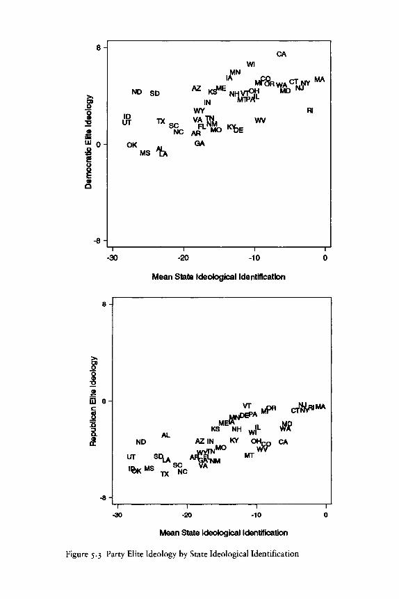
i
8 -
- 8 -
ND SD
ID _ ,UT TX
OK A |
MS T!>
SCNC
INWY
GA
NHVMl
Wl
MPS
WV
CA
Tft>Rl
-30 -20 -10
Mean State Ideological Identification
8 -
03 0 -
In
- 8 -
^ A M P " crVA""
ALND
UT S C ^
l«g>KMS7X
SCNC
KSIW"" NH w j L MRAZIN KY OHgo CA
MT
-30 -20 -10
Mean State Ideological Identification
Figure 5.3 Party Elite Ideology by State Ideological Identification

Statehouse democracy
However, there is a quite satisfactory resolution of this shortfall. If weadjust for the measurement error in state opinion, the expected resultappears. We can see this quite simply by dividing the states into two equalportions based on the sample size for the state opinion measure. (The halfof the states with more respondents in the 13-year sample all have over2,110 respondents.) In the states with larger, more reliable samples, thecorrelation between the two party elite measures is .67, about the same aswe found for the total sample. For these states, state opinion correlates ata very strong .82 and .83 with Democratic and Republican elite ide-ologies, respectively. The product of these two numbers, .68, is actually apoint larger than the target value of .67. We can readily conclude that forstates with minimal measurement error, the influence of state opinionfully accounts for the correlation between state Democratic elite ideologyand state Republican elite ideology. Meanwhile, for that half of the stateswith lesser sample sizes, the two party elite measures correlate at .59,offering satisfaction that these two measures are not attenuated for rela-tively unpopulous states. But due to the sampling error in the opinionmeasure, the Democratic and Republican elite measures correlate at only.42 and .73, respectively, with state opinion. The product equals a mere.31, but we partially attribute this low number to sampling error in theselection of states with small sample sizes for the opinion measure.
ACTIVIST ELITES, ELECTORAL ELITES, AND STATE
OPINION
We can also separate out the state opinion-party elite correlations foractivist elites (convention delegates and county chairpersons) and for elec-toral elites (state legislators and congressional candidates). Electoral lead-ers face the incentive to shade toward moderation, away from their party'sideological extreme. The amount of this pressure should be a function ofstate liberalism-conservatism. A Democratic candidate, for example,would be more pressured to moderate in a state with conservative votersthan one with liberal voters. Of course, the same applies to a Republicanin the other direction; the strength of the pull away from conservativeextremism should be proportional to the liberalism of the state. Activistsshould feel this pressure much less, if at all.
The correlations shown in Table 5.4 and pictured in Figure 5.4 supportthese conjectures. State opinion more strongly correlates with the ide-ologies of electoral elites than that of activists. We can also examine themeasures of elite opinion as a function of both state opinion and partyaffiliation. This entails pooling Democratic and Republican party elites inthe same data set (N = states x 2 = 92). Table 5.5 shows a set of regressionsthat tells an interesting story. We regress both activist and electoral elite
108

Democratic elites
.37
.70
.62
Republican elites
.60
.78
.77
State parties and state opinion
Table 5.4. Correlations between elite ideology and state opinion
Elite type
Activist
Electoral
Overall
Note: Table entries are Pearson product moment correlations between the ideology score foreach elite group and state opinion liberalism.
ideologies on state opinion and party. Compare Equation l for activistideology and Equation z for electoral elite ideology. That comparisonshows that activist ideologies are the more responsive to party (3.61 vs.2.75) while electoral elite ideologies are the more responsive to state opin-ion (.05 vs. .13). Equation 3, with electoral elite ideology as the dependentvariable, has activist opinion as an explanatory variable, along with stateopinion and party affiliation. Here, the coefficient for party actuallyvanishes-it changes sign and is not statistically significant. This meansthat the addition of activist opinion to the analysis completely explains thepartisan differences between Democratic and Republican electoral elites.Here, then, we obtain firm empirical evidence for what "party" meanswhen we say, for example, that party affiliation is an important variable inlegislative policy making. "Party" in this sense stands for the issue stancesand ideological values of the self-recruiting issue-motivated party elites inthe states and districts in which legislators develop their political careers,get nominated, and eventually get elected. (See Wright, 1989 for parallelevidence in the case of roll call voting in the U.S. Senate.)
This points to an important - indeed fundamental - finding about stateparties. The values and ideologies of party activists are what give shapeand definition to what the parties stand for in state politics. There isconsiderable variation across the states in the relative liberalism-conservatism of party activists, and these differences are only weakly cor-related with public opinion in the states. While we do find that electoralelites take moderate positions more congruent with those of voters nearthe ideological center of their states, we also find a remarkably powerfuleffect for activists in influencing the ideological positions of state electoralelites.
109

Statehouse democracy
8D
ND
TX
IDUTOK
M8 &
8CNC
[
A Z , ^
M
AJ^MCA^MCGA
CA
Wl CT ^IA,N CO NV
OHftR̂ JJ W
* • # -WV
DE»KY
-20 -10 0Mean Ideological Identification
-30 -20 -10 0Mean Ideological Identification
-30 -20 -10 0
Mean Ideological Identification
-30 -20 -10 0
Mean Ideological Identification
Figure 5.4 Party Activist and Electoral Elite Ideology by State Ideology
n o

State parties and state opinion
Table 5.5. Regressions of state elite ideology on state opinion and party
Independentvariable
Party(Democrats;Republican=O)
Activist ideology
(1)
b Beta
3.61* 0.93
(2)
b
2.75*
Electoral elite ideology
Beta
0.73
(3)
b Beta
-1.41 -0.11
(4)
b Beta
State 0.05* 0.18 0.13* 0.51 0.09* 0.35 0.10* 0.37Opinion
Activist 0.87* 0.90 0.77* 0.80Ideology
Adjusted/?2 .891 .782 .870 .870
Note: N=92.* significant at .001. 6's without asterisks are not significant, even at the .05 level.
A further question is whether, when electoral elites respond to stateopinion, they weigh the opinions of different kinds of partisansdifferently. Since activists are drawn from the state pools of party identi-fiers, we would expect that activists would represent mainly their ownpartisan grouping. Electoral elites may have a Downsian incentive toweigh the views of Independents higher because electoral marginalitymakes them a crucial swing group (Wright, 1989; Erikson and Romero,1990). Testing these conjectures carries us toward the limits of what ourdata might be expected to reveal. Yet the data are generally supportive ofour speculation.
Table 5.6 shows the two sets of elites (activists and elected officials) as afunction of state opinion once more, but this time opinion is divided intothe ideological means for three groups - their own party, the oppositeparty, and Independents. Opinion is weighted in proportion to eachgroup's share of the electorate, so that any inequity in the coefficientsrepresents only the differential weighting for the three partisan groups,and not their proportions of the electorate. In Table 5.6, for electoral eliteswe also include party activists' mean ideology.
in

Statehouse democracy
Table 5.6. Regressions of elite ideology on party and state opinion, bypartisan groupings
Activist Electoral EliteIdeology Ideology
Variable (1) (2) (3) (4)
Party 2.83** 1.61** -0.81(Democrat= 1;Republican = 0)
Same party opinion 0.08** 0.16** 0.09** 0.09*x Same party proportionof state electorate
Opposition party opinion 0.00 0.05 0.04 0.06*x Opposition party proportionof state electorate
Independent opinion 0.04 0.17** 0.13** 0.14**x Independent proportionof state electorate
Activist opinion 0.85** 0.72**
Adjusted/?2 .894a .790a .870 .867
Note: Coefficients are unstandardized b's.* Significant at .01; **significant at .001.•Significant (.05) improvement over the base equation where Democratic, Republican, andIndependent opinions are weighted equally.
The activist equation (Equation l) is remarkably consistent with ourexpectations. Activist opinion within a state party is a function of partyaffiliation and the opinions of the activists' rank-and-file partisans. Butaccording to the equation, opinions of the opposition party's partisansand of Independents do not matter.
Equations 2, 3, and 4 present a different story for electoral elites. Mir-roring Table 5.5, they show that electoral elites respond to both activistopinion within their party and state opinion at large. With state opiniondivided into three partisan categories, we see that opinions of Indepen-dents appears marginally more important than partisan opinions. Al-
112

State parties and state opinion
though not statistically significant, this tendency is in the direction pre-dicted. But Independent opinion is not all that matters. When activistopinion is omitted (Equation 2), "same party" opinion mattersconsiderably - reflecting an indirect effect via activists. On net balance,opposition party opinion matters least in determining the opinions ofelectoral elites.
In summary, the ideological postures of electoral elites represent a com-promise between the ideological preferences of party activists and themoderating forces needed to get elected. State electoral elites present acomposite of activist opinion plus mass opinion. The data present anintriguing but modest hint that electoral elites weigh the opinions of Inde-pendent swing voters most heavily. But electoral elites' own partisan vot-ers are influential indirectly, because they comprise the pool from whichactivists are drawn. The electorate's task is to distribute the two contestingsets of elites into office, in proportion to their representation of massideological preferences. That performance is the subject of subsequentchapters.
PARTY MIDPOINT AND PARTY POLARIZATION
In addition to separately scoring the individual Democratic and Republi-can elites of the states, we can classify states according to their combina-tion of Democratic and Republican elite ideologies. There are two ways tocombine the elite measures to score the party "system." One obvious wayis to simply average the ideologies of the two party elites. We refer to thisaverage as the "party midpoint." A second measure is the ideologicaldistance between the two party elites. We refer to this as the "polariza-tion" score for state parties. For any given party midpoint, any value ofparty polarization is theoretically possible. Consider, for instance, a cen-trist party midpoint. In the case of Downsian parties offering centristpolicies, the moderate party midpoint would be accompanied by a lowlevel of polarization. However, with parties behaving in the responsibleparties fashion, parties could on average present a centrist midpoint butwith a polarized ideological choice.4
The midpoint and the polarization scores are shown graphically in thescatterplot of Figure 5.5. We can divide the states into four types as repre-sented by particular states. Vermont for example has a relatively liberaland relatively unpolarized party system. At the opposite extreme,
4. The party midpoint is the mean of the Democratic and Republican "overall" scoresreported in Table 5.3. The party elite polarization index is the difference betweenthese two overall scores. The polarization measure can be divided into its fourcomponents - the party difference on each of the four elite measures. These fourpolarization components are modestly correlated, with an average intercorrelationof.23.
113

Statehouse democracy
3 -
2 -
1 -
0 -
TX ID
NC SCVANMUT
°K AR M(
MS GALA
AL
SD COMT AZ
WY NCPH
IN iXM Nf
KY
f
DE
?MEiMD
PA
Rl
CA
Wl
J|«NMl
NYORA
NJVT
I-4
I
-2i
0
Party Elite Midpoint
Figure 5.5 Party Elite Polarization and Party Elite Midpoints.
Texas is an example of a relatively conservative and relatively polarizedparty system. California and Wisconsin exemplify states that are liberaland polarized. Opposite from them is Louisiana, conservative and un-polarized. Each type, one might anticipate, enjoys a somewhat distinctbrand of politics - in terms of contentiousness and predictability of thepolicy process.
Since the party midpoint is simply the average of the Republican andDemocratic elite positions for the state, like its two components it shouldcorrelate strongly with state opinion. Indeed, this correlation is a healthy.76. We have strong reason to suspect that this correlation would be muchhigher if measurement error in state opinion were removed. Dividing thestates in two groups based on state opinion sample size, we find that themidpoint correlates at a very high .90 for the 23 states with sample sizesabove 2,110 and a lesser .64 for the remainder.
We would not expect party polarization to correlate with the directionof opinion, and it does not. The correlation is a meaningless -.05. Partyelite polarization should correlate, however, with the polarization of stateopinion. Recall from Chapter 2 our measure of mass polarization as thedifference between the mean ideology of a state's Democratic identifiers
114

State parties and state opinion
and the mean ideology of the state's Republican identifiers. This variabledoes correlate with party polarization at a modest .42. We expect thisobserved correlation to be attenuated due to measurement error, so thatits moderate magnitude may indicate an interesting effect. To explore thisfurther, we estimate the correlation between the estimated mass polariza-tion and party polarization for the 23 states with the largest CBS/NYTsurvey samples. Now we find the correlation rises to a much higher .65.(For the 23 states with lesser sample sizes, the correlation falls to .20.)Thus we have identified a major source of party polarization. When thestate electorate is polarized ideologically, so too are the party elites.
PARTY SYSTEMS AND PARTY CONFLICT
Several studies have classified political systems in the U.S. states accordingto the nature of state political conflict. Here, we assess the relationshipsbetween our classification of party systems based on our measurement ofparty elite ideology on the one hand, and the relevant classificationschemes found in the literature, on the other. Whereas our ideologicalmeasurement of state parties is based on composite surveys of party elites,other researchers have inferred party differences from patterns of policymaking or from relatively unsystematic observations of the states andtheir parties. We will contrast our measures with the party classificationsoffered by John Fenton (1966), Edward Jennings (1979), Thomas Dye(1984), and James Garand (1985). Each of these scholars has provided aclassification of states based on a dimension of substantive differencesbetween the parties.5
The first two classifications we consider include only a few states each.John Fenton's classic study, Midwest Politics (1966), examines six states,classifying three as primarily "issue-oriented" (Michigan, Wisconsin, andMinnesota) and three as primarily "job-oriented" (Illinois, Indiana, andOhio). This division nicely parallels the distinction between the "newstyle" and "old style" politics described by Sorauf and Beck (1988, chap.16) and dovetails nicely with the theoretical distinction between responsi-ble parties (more issue-oriented elites) and Downsian parties (more prag-matic elites). Thus, we anticipate greater levels of party polarization in theissue-oriented states than in the job-oriented states.
A similar distinction is pursued by Edward Jennings (1979), whoclassifies eight states as "class-based" or "non-class-based" over theperiod 193 2-70. Jennings reports some of the strongest evidence availablethat policies change when the voters change the governing party - but
5. Some readers might expect us to include Daniel Elazar's (1966, 1972) typology ofstates according to political culture in our analysis here. We present a detailed analy-sis of Elazar's model in Chapter 7.
" 5

Statehouse democracy
only when the parties are clearly different on policies. Two of the states inJennings' analysis changed the nature of their politics, and hence theirclassification, during the period. We use his classification as of the end ofthat period. From Jennings's discussion it is clear that his nonclass-basedparties are nonideological more generally. They battle for the patronagespoils of office rather then for high principles of governance. We wouldexpect to find, therefore, higher polarization scores among Jennings'sclass-based party states.
Thomas Dye's (1966) research on comparative state politics has helpedto set the agenda for much of the subsequent work in the field. Dye foundthat measures of economic development of the states were better predic-tors of state expenditure policies than were available measures of politicalvariables, such as relative strengths of the two parties. Our explanationfor why political parties do not matter is that the parties may stand fordifferent things in different places. Dye (1984) expands on this observa-tion to make the argument - similar in spirit to that offered by Jennings -that party control will matter only when the policy programs and electoralconstituencies of the parties are significantly different from each another.Accordingly, Dye offers a classification of the states based on whethertheir parties were "policy relevant." He bases this classification on a time-series analysis of when welfare expenditures change with party control.When the changes are in the expected direction - expenditures go up whenDemocrats come into office or down when Republicans come into office -the parties are deemed to be policy relevant. When the expected policychange does not occur, Dye concludes that the parties are not policy rele-vant. Our hypothesis is the obvious: Party polarization should be largeramong the states Dye classifies as policy relevant.
James Garand (1985) takes a similar theoretical approach as Dye butuses a different basis for classifying the states. From his survey of theliterature, Garand combines the various descriptions of the states into ascale of "policy differentiation" between the parties. He finds some of thestates have high levels of policy differentiation between the parties, othersmedium, and still others low differentiation. Garand's measure presents astrong parallel, conceptually, to our measure of party polarization: Statesgiven scores of high levels of policy differentiation should be our stateswith the greatest ideological polarization of party elites.
The analysis of these four classifications in terms of our party systemvariables is shown in Table 5.7. For each we have a clear hypothesis thatpolarization scores should be higher in systems that posit greater partydistances. For the most part, however, we have no hypothesis about themidpoint of party elite ideology; there is no a priori reason to expect arelationship between the relevance of issues to the parties and the direc-tion, liberal or conservative, of the party system.
116

State parties and state opinion
Table 5.7. Party elite liberalism and party polarization by selected partyclassifications
Classifications ofState Party Systems
Party EliteLiberalism
PartyPolarization
Fenton (1966)
Issue-oriented (Af=3)Job-oriented (N=3)
Significance
2.17.43
Fx 4=69.5***
7.526.95
F,4=0.28
Jennings (1979)
Class-based (N=6)Nonclass-based (A/=2)
Significance
1.61-1.33
^.6=5.0
6.945.60
Dye (1984)
Policy-relevant (JV=18)Not policy-relevant (N=29)
Significance
.94-.57
FM5=10.2**
6.936.00
^1,45=3.4
Garand (1985)
Policy Differentiation:High (JV=15)Moderate (N=16)Low (N=16)
Significance
1.60-.13
-1.35
F2)44=21.3***
6.186.726.16
F2M=0.5l
Note: Table entries are category means.•Significant at .05; **significant at.01; ***significant at .001.
1 1 7

Statehouse democracy
The pattern that we find in Table 5.7 is quite intriguing. Our primaryhypothesis, that there should be a relationship between our polarizationmeasure and the classification systems, received no support in any of thefour tests. Some of the relationships are in the predicted direction, butthey are small and not statistically significant. Overall, party ideologicaldistances do not coincide with the classification schemes of the literature.
The other surprise is that the party elite ideological midpoints do coin-cide with the various classification schemes. In all four tests, where theparties are believed to be more ideological or issue/class-oriented we findthat the party systems are significantly more liberal. The theoretical rever-sal here is remarkable. We had strong theoretical reasons to expect polar-ization to be related to party classification, and instead we find that partyelite liberalism is - and this occurs with striking consistency across frame-works developed over quite a time period and with quite different meth-ods.
How is it that a set of keen observers of state politics could think theywere seeing class-based or issue-based differences in the party systems,whereas what they really distinguish is the overall liberalism-conservatism of the party systems? It could be that these observers werejust wrong, that they did not know what they were seeing when theylooked at state politics. Such a conclusion would be hasty, perhaps imper-tinent, and worse, it would leave us with no explanation for the patternthat we do find. Instead, let us review our findings again. We expected tofind that the policy distances between the parties would be larger inpolicy-oriented or class-based party systems. This does not turn out to bethe case. Rather, our panel of highly informed observers have identifiedstates with liberal party elites as the states possessing strong class or policydivision between the parties.
What is actually varying, then, in these classification schemes is not theideological distance between party elites, but rather the location on theideological spectrum where the most salient party conflict occurs. Here,we believe, is the resolution to the puzzle. For a party system to be called"class-based" or "policy-relevant," political scientists are conditioned tolook for partisan division over classic issues of redistribution. For such apartisan division, the more liberal (Democratic) party must visibly appealto the have-nots, welfare recipients or other groups whose interests con-stitute class-based or policy-relevant politics. Where the parties are moreconservative, not even the Democratic Party facilitates the expression ofthe interests of the have-nots. Conservative party systems may containsubstantial ideological gaps between the parties, but the division is simplyto the right of the ideological zone generally identified with meaningfulissue or class conflict. Arguably, these less visible divisions have been toolong ignored. Perhaps state policy analysts should give greater consider-
118
State parties and state opinion
ation to variability in the policy concerns of the constituencies of the twoparties across the states, not just where obvious class conflict is manifest.
CONCLUSIONS
This chapter has shown that the ideologies represented by the state partyelites are a reflection of state opinion. Democratic elites are to the public'sleft, and Republican elites are to the public's right. But within each party,the degree of liberalism among the leadership is correlated with the degreeof liberalism of the state public. The process is complex. Party activists aredrawn from the state public at large, with liberals moving into theDemocratic elite and conservatives into the Republican elite. Each party'selectoral elite must respond not only to activist sentiment but also to theviews of the electorate. The electorate's complicated task is to sort this allout. From the conflicting programs of Democratic and Republican par-ties, both perhaps too extreme for average tastes, the electorate must dothe proper sorting to determine who gets elected and who does not. Insubsequent chapters, we will see how the electorate's performance of thistask is an important part of the electoral process.
1 1 9

Legislative elections and state policy
One central question about modern democracies is, How much do par-tisan elections contribute to the effective representation of public opin-ion? In theory, programmatic parties provide the electorate with a clearchoice of policy options, with election results followed by predictablepolicy consequences. But empirically, does it matter which party (or coali-tion) governs? Most recent cross-national comparisons of Westerndemocracies answer affirmatively. Socialist or leftist party participation innational governments is associated with a high inflation to unemploymenttradeoff (Hibbs, 1977), growth of the governmental sector (Cameron,1978; Lange and Garrett, 1985), high public expenditure (Tufte, 1978;Castles, 1982), welfare spending (Castles, 1982; Hicks and Swank, 1984),quality-of-life (Moon and Dixon 1985), and income equality/redistribution (Tufte, 1978; van Arnhem, Corina, and Schotsman, 1982;but see also, Jackman, 1975, 1980). In sum> nations where leftist partiesare most influential also tend to have the kinds of policies and policyconsequences with the greatest appeal to leftist constituencies. Time-seriesanalyses for individual nations also show policy consequences resultingfrom party control (Hibbs, 1977, 1987; Alt, 1985). Party control doesmatter.
It may be the case, however, that party control matters only in terms ofthe sharp divisions between European socialist parties of the left and par-ties of the right. In the U.S. context, it is by no means clear that majorpolicy differences flow from variation in Democratic versus Republicancontrol. At the national level, while some time series find policy conse-quences from party control of the presidency and/or Congress (Hibbs,1977,1987; Kiewiet and McCubbins, 1985), the role of parties remains insome dispute (Beck, 1982; Browning, 1985; Lowery, 1985).
At the state level, the policy relevance of party control has been viewedwith particular skepticism. Indeed, in state policy research, the apparentirrelevance of political parties has been a persistent puzzle. Presumably,
120

Legislative elections and state policy
Republican states would have the most conservative policies andDemocratic states the most liberal policies. But this is not the case. Therelative strengths of the Republican and Democratic parties in state poli-tics appear to be statistically unrelated to policy directions in the states,even after the imposition of rigorous controls (Dye, 1966; Winters, 1976;Plotnick and Winters, 1985). Only time-series analyses show any evidenceof the expected party effects, with welfare spending responsive to partycontrol in some states but perhaps not in others (Jennings, 1979; Dye,1984; Garand, 1985).
The nonrelationship between party control and state policy appears todeny common, seemingly informed, stereotypes of how politics in theUnited States works. Most observers would agree that Democratic andRepublican elites differ ideologically in terms of their political values andas manifested in certain behaviors such as roll call votes. Could this be anillusion? Could it be that the two parties have become indistinguishable onpolicy substance, just what spatial models of party competition predictshould happen with electorally driven parties (Downs, 1957)? Clearly theanswer is no. As Chapter 5 showed, Democratic and Republican partyelites are quite ideologically distinct in individual states. If party controlmakes no difference, the reason is not that the leaderships of the twoparties are not ideologically different.
Then, perhaps the seeming irrelevance of parties is confirmation of thegeneral theory that policy outcomes are determined by environmentalrather than political variables (Dye, 1966, 1979). Indeed, the failure ofparty control to predict policy may be the strongest evidence available insupport of the environmental theory. Although Republican and Democra-tic candidates diverge in their campaign rhetoric and even in their person-al values, perhaps Republican and Democratic politicians ultimately enactthe same policies when given the responsibility of governing. By this sce-nario, politicians in office respond to the social needs and economic con-straints of the state at the expense of campaign pledges or other ephemeralpolitical considerations.
A BROKEN ELECTORAL LINKAGE?
Does electoral politics in the states really not matter? Consider our .82correlation between the net ideological identification of state opinion andour composite measure of state policy liberalism. Clearly, the ideologicalpreferences of state electorates play an important role in determining theideological tone of state policies. Partisan elections would seem a likelyconduit for this flow of causality, with liberal states electing Democratswho enact liberal legislation and conservative states electing Republicanswho enact conservative legislation. This simple model is diagramed inFigure 6.1.
121

Statehouse democracy
But our data do not fit this simple model. Echoing earlier findings, wefind Democratic Party control of state legislatures unrelated (r = -.22) toour eight-item measure of state policy liberalism (described in Chapter 4).Moreover, even if party control could account for policy, the linkage be-tween opinion and policy via parties would be broken at the front end.The correlation between the liberalism of state publics and Democraticcontrol is only .01. Thus, liberal and conservative states do not differ intheir tendencies to elect Republicans or Democrats to state office. Thestrong effect of state opinion on state policy would seem to bypass theelectoral process.
State-to-state differences in mean party identification add to the puzzle.Not only are the ideological preferences of state electorates uncorrelatedwith the partisan composition of state elected officials, but they are alsounrelated to the electorate's partisan preferences. The mean liberalism ofstate public opinion correlates at only .06 with mean Democratic Partyidentification. State party identification, however, does correlate with par-ty control (r = .87) just as one would think that it must.
Democratic states do elect the most Democrats to state office. But themost Democratic state electorates are not unusually liberal. And theDemocratic legislatures they elect do not enact unusually liberal legisla-tion. All this would seem to deny the presence of much policy representa-tion. But we must remember that the most liberal state electorates do electlegislators who enact the most liberal legislation, even with the absence ofany obvious partisan linkage.
Are political parties as irrelevant to the representation process as thisanalysis suggests? Perhaps political parties do play an important role: It isjust that the linkage is more complicated than we have presented so far.But to pursue this possibility, we must have a theory of how partisanelections fit into the representation process in the states. In the next sec-tion, we attempt to develop this theory.
A THEORY OF STATE ELECTORAL POLITICS
A theory of state electoral politics must take into account the wide varia-tion in the ideological orientations of state political parties. To take anobvious example, the Democratic Party of Mississippi is far more conser-vative than the Democratic Party of New York, and perhaps the NewYork Republican Party as well. With the Democratic and the Republicanparties each differing ideologically from one state to the next, the potentialexists for serious confounding of our understanding of how parties con-tribute to the policy representation in the states. This ideological variationof state parties sometimes appears to be chaotic and idiosyncratic to par-ticular state political cultures. But as we have already seen in Chapter 5,
122

Legislative elections and state policy
Opinion ^ Democratic ^ PolicyLiberalism Party Control Liberalism
Figure 6.1 A Simple Model of State Public Opinion andPolicy
considerable order and predictability exists, with the ideologies of stateparty elites a function of the particular party and electoral constituencies.
To develop some propositions about state party ideology, party elec-toral strength, and state policy, let us take the role of elections in the policyprocess seriously. Suppose that state electorates actually reward and pun-ish the parties on the basis of their policy positions and specifically on thebasis of their placement on the left-right continuum. That is, suppose thatstate electorates tend to reward the party that best reflects their ideologicalviewpoints. Suppose also that state parties are motivated (at least in part)to win elections. Then, to the extent parties are electorally motivated, theyshould respond to state opinion. To the extent parties respond effectivelyto state opinion, they should achieve electoral success.
Chapter 5 has presented evidence of parties responding to state opin-ion. Relatively conservative states draw relatively conservative Democra-tic and Republican elites and relatively liberal states draw relatively liberalDemocratic and Republican elites. At the same time, state parties are notdriven entirely by state opinion. If they were, state parties would alwaysconverge to the position of the state's median voter. In actuality stateparties, like national parties, are pushed toward the median voter positionby electoral considerations and away from the median voter position bythe preferences of their activists.
The ideological motivations of state party elites were the focus of theprevious chapter. The present chapter focuses on the response of stateelectorates to the ideological alternatives presented by competingDemocratic and Republican elites. To the extent state elections aredecided by ideology, state electoral success should go to the party that isideologically closest to the state electorate. Thus, Republican state partiesshould be most successful when they move toward the liberalism of theDemocratic opposition. Democratic state parties should be most success-ful when they move toward the conservatism of the Republican opposi-tion. These policies could backfire, but only if the parties move too far, aswhen the Democrats get so conservative that the Republicans outflankthem on the left. But as we saw in Chapter 5, this does not happen withstate parties.
To summarize, it is the ideological flexibility of the Democratic andRepublican parties in the states that obscures the linkage between party
123

Statehouse democracy
control and public policy in the states. As seen in the previous chapter,ideologically flexible parties respond to state public opinion even as theytry to satisfy their own ideological furies. As we will see in this chapter,parties are electorally rewarded and punished based on how well theyrepresent state opinion.1
Our argument can be recognized as a continuation from Chapter 5 ofthe Downsian (Downs, 1957) theme that electoral rewards lie in the politi-cal center. Appendix A to this chapter explicates the formal argument ingreater detail and, with hypothetical examples, illustrates the proposi-tions described in the following section, where we explore the implica-tions for estimating the role of party control in the representation processin the states.
A model of electoral representation
According to our model, centrist parties are electorally rewarded. Thismeans that the Democrats are rewarded for movement in the conservativedirection and the Republicans for movement in the liberal direction.2 Inbrief, liberal parties (Democratic or Republican) negatively affectDemocratic success. Figure 6.2 introduces party positions to the model ofstate electoral representation. Let us consider how electorally responsiveparties can contribute to representation and at the same time account forthe absence of correlations between opinion liberalism and Democraticsuccess and between Democratic success and policy liberalism.
In our model, liberal opinion causes liberal parties. However, whenstate electorates respond to party positions, liberal parties hinderDemocratic success. This makes a negative indirect path from opinionliberalism to Democratic control. At the same time, the model shows apositive direct effect of opinion liberalism on Democratic legislative
1. This argument may apply to cross-national comparisons as well. The U.S. Democra-tic Party is more ideologically centrist than parties of the Left in Europe and moresuccessful electorally. One may wonder, therefore, whether the relative electoralsuccess of the Left but nonsocialist U.S. Democrats (and also the Canadian Liberals)disturbs the cross-national relationship between leftist party success and policy.However, cross-national studies do not code the nonsocialist U.S. Democrats andCanadian Liberals as parties of the Left. The Left designation is reserved for ex-plicitly Socialist or Social Democratic parties. If cross-national studies were to codethe U.S. Democrats and Canadian Liberals as successful leftist parties, cross-nationalrelationships between party control and policy would become seriously attenuated.
2. We speak somewhat loosely about movement to the political "center." Strictlyspeaking, attempting to observe whether parties are at the political center wouldrequire a common metric for parties and the electorate. In actuality, the location ofthe "center" is irrelevant since each party should be electorally rewarded for movingtoward the ideological position of its opposition, whatever side of "center." SeeAppendix A.
124

Legislative elections and state policy
Party EliteLiberalism
Opinion
Liberalism
Democratic
Party Control
Figure 6.2 Representation Model with Party Elites
strength. The net effect of the combined indirect and direct paths couldwell be a low bivariate correlation between state opinion and party con-trol.
The model also accounts for the low correlation between party controland policy. According to the model, party ideology suppresses the positiverelationship between party control and policy: Liberal parties workagainst Democratic control but for liberal policies. This source of spu-rious negative correlation obscures the posited positive effect of Democra-tic control on liberal policy.
Figure 6.2 also shows how parties' responsiveness to state opinion con-tributes to representation in a rather straightforward fashion. Liberalstate opinion causes liberal state party elites, which result in liberal pol-icies. But also, the combination of state opinion and party elite ideologydetermine party control, which also determines policy. Finally, the modelallows for the direct effect of opinion on policy independent of partisanvariables.
The model can be complicated further. Figure 6.3 adds two more vari-ables: state party identification and the liberalism of the state legislature.Figure 6.3 also adds specificity to the meaning of party control by redefin-ing it in terms of Democratic legislative strength.
This new model places party identification as an intervening variablebetween opinion liberalism and Democratic legislative strength. Partisan-ship provides a mechanism for translating public opinion into legislativepower: Liberal states tend to identify with the Democratic Party, whichincreases the number of Democratic state legislators. Surprisingly, as pre-viously reported, the correlation between opinion liberalism andDemocratic party identification in the states is virtually zero. But the roleof party elites can explain this anomaly: Liberal states cause liberal parties,which over time contribute negatively to Democratic partisanship. Thiseffect hides the expected relationship between public opinion and par-tisanship in which liberals tend to identify with the Democratic Party.
The liberalism of the legislature is introduced as an intervening variablecaused by the degree of liberalism among the two major parties' elites and
125

Statehouse democracy
Party EliteLiberalism
Opinion
Liberalism
LegislativeLiberalism
Policy
Liberalism
DemocraticParty Identification
DemocraticLegislative Strength
Figure 6.3 Model of the Policy Process
the partisan division of the legislature: The more liberal the parties and themore Democrats in the legislature, the more liberal should be the legisla-ture. The inclusion of legislative liberalism provides an additional subtletyto the model. Electing Democrats should liberalize the legislature, whichleads to liberal policies. But as Figure 6.3 suggests, with legislative liberal-ism and public liberalism held constant, the residual direct effect on policyliberalism of electing Democrats is posited to be negative.
The ceteris paribus condition is crucial for this proposition. We do notseriously speculate that electing Republicans is the way to get liberal pol-icies (although speculation of that sort can be found in the literature, seeGoodin, 1983). Rather, under identical political circumstances and withidentical ideological values, Republican and Democratic legislatorsshould respond in different directions to electoral motivations: Republi-cans should find more votes by moving left and Democrats should findmore votes by moving right. Of course, Republican and Democratic legis-lators tend to differ in their ideological values. But conceivably, electoralmotivations could be so strong that conservative Republicans and liberalDemocrats make ideologically similar decisions when in control of thestate legislatures.
In summary, the model of Figure 6.3 shows how state opinion can influ-ence state policy via a variety of indirect electoral pathways. These path-ways are based on the assumptions that state parties respond to stateopinion and that state electorates respond to party positions. If this the-oretical development is correct, electoral politics can be crucial for policyrepresentation in the states, even though party control is statistically un-correlated with both state opinion and state policy.
One important omission from this model is the governor and his role instate policy. This omission is due largely to measurement considerationsrather than disregard for the governor's role in the legislative process.When the dependent variable is a set of policies cumulated from years of
126

Legislative elections and state policy
legislative decision-making, it makes little sense to include the governor'sparty affiliation for the short term as an independent variable. And par-tisan control of governorships over the long term bears little relationshipto other indicators of partisanship. Where unusual long-term success for aparty is found at the gubernatorial level (e.g., Utah for the Democrats,Michigan for the Republicans), this may result precisely because of guber-natorial leadership that is ideologically atypical for the party. We are farmore reluctant to assume that governors share the ideological positionsmeasured for their party's elite than we are that, on the average, statelegislators do so.
While we do not include the state's chief executive in our model formeasurement reasons, this decision should not significantly distort themodel we present. Much has been made in recent years of the increasingformal authority of governors. Yet little evidence exists that demonstratesan empirical link between the powers of the executive and actual policydirection. For instance, state representatives rarely see the governor asplaying a significant role in the state legislature. Legislators rank the gov-ernor last among 13 potential decision cue sources: Less than 2 percent ofall state legislators choose the governor as the principal informant fortheir decisions (Uslaner and Weber, 1977, 34).
MEASUREMENT
To put the theory to use, it is necessary to operationalize each of thecomponent parts. State opinion (Chapter 2), state party identification(Chapter 2), states' composite policy liberalism (Chapter 4), and partyelite ideology (Chapter 5) have all been introduced previously. Of these,only one - party elite ideology - requires additional discussion here.
Party elite ideology was presented as a composite of the ideologicalpositions of county chairpersons, national convention delegates, membersof Congress, and state legislative candidates. The former two componentstap the ideology of the activist party elites, and the latter two the ideologyof the electoral party elites. As Chapter 5 showed, electoral elite ideologyis more responsive to state opinion than is activist elite ideology. For thischapter, we use the composite measure of party elite ideology, therebycombining the views of activists and electoral elites. We do so because asindependent variables affecting state elections and state policy, the twocannot be statistically disentangled. That is, based on statistical evidence,state publics view state party positions as a composite of the parties' activ-ist elites and electoral elites. Also, the two components appear to haveequal effects on state policy. Here we further reduce the measure of partyelite ideology to its essentials, by averaging the Republican and Democra-tic elite ideology scores as the party midpoint.
127

Statehouse democracy
Table 6.1. Correlations among variables for model of state policy process:46 states
Party Democratic DemocraticOpinion elite party legislative Legislative Policy
Variables liberalism liberalism identification strength liberalism liberalism
Opinionliberalism 1.00 .76 .06 .01 .82 .83
Party eliteliberalism 1.00 -.37 -.42 .79 .85
Democratic partyidentification 1.00 .87 .15 -.20
Democratic legislativestrength 1.00 .19 -.22
Legislativeliberalism 1.00 .78
Policyliberalism 1.00
Note: N=46. Alaska, Hawaii, Nebraska, and Nevada are excluded.
Two variables that do require introduction in this chapter are Democra-tic "legislative strength" and "legislative ideology." Democratic state leg-islative strength is measured as the average of the Democratic strength foreach legislative chamber over the 1977-84 period. Upper and lowerchambers are weighted equally.
Legislative ideology is a more difficult challenge, requiring indirectmeasurement. We operationalize legislative liberalism as the weightedaverage of the Democratic and Republican elite ideology scores, where theweights are determined by the parties' relative legislative strength (weigh-ing the two chambers equally). In other words, we assume that the averageliberalism of a state's Democratic legislators is the mean composite liberal-ism score for the state's Democratic elite; and we assume that the averageliberalism of a state's Republican legislators is the mean composite liberal-ism score for the state's Republican elite. Democratic and Republicancomposite ideology scores are then combined in proportion to the twoparties' average legislative strength.
128

Legislative elections and state policy
Table 6.2. Standardized regressions for path model of policy process: 46states
Independentvariables
Opinionliberalism
Party eliteliberalism
Partyelite
liberalism
0.76*(0.10)
Democratic partyidentification
Democratic legislativestrength
Legislativeliberalism
Adjusted R2 .573
Dependent variables
Democratic Democraticparty legislative
identification strength
0.83*(0.18)
-1.01*(0.18)
.404
0.15(0.14)
-0.24(0.15)
0.78*(0.10)
.760
Legislativeliberalism
1.05*(0.04)
0.63*(0.04)
.948
Policyliberalism
0.44*(0.12)
-0.32*(0.07)
0.48*(0.12)
.799
Note: N=46. Alaska, Hawaii, Nebraska, and Nevada are excluded. Standard errors inparentheses.•Significant at .001.
The following sections report on the empirical fit of the causal modelpresented in Figure 6.3. For handy reference to these sections, Table 6.1reports the correlation matrix for the variables; Table 6.2 shows the re-sults of the standardized regression equations; Figure 6.4 shows the causalmodel with the estimated standardized path coefficients (betas) included.3
A case can also be made for doing the analysis without the potentially
3. With Nebraska omitted, the opinion-policy correlation rises minisculely from .82to .83. Certain arrows (e.g., from party identification to legislative liberalism) aredeleted from Figure 6.4, on the grounds that the expected direct effect is zero.Technically speaking, therefore, Figure 6.4 presents an over identified model. Inclu-sion of the omitted effects would be of little consequence other than to clutter theanalysis with small theoretically meaningless coefficients.
129

Statehouse democracy
0.44
Party EliteLiberalism
1.05
State Opinion
Liberalism
0.83XState Democratic
Party Identification0.77
Legislative
Liberalism >. o.48
P o l i cy
Liberalism- 0 . 3 2 ^
DemocraticLegislative Strength
Figure 6.4 Path Model of the State Policy Process (46 states)
confounding (and interactive) effects of southern regionalism. According-ly, we present a brief parallel analysis in Appendix B, with southern statesremoved.
PUBLIC OPINION AND PARTY ELITES
First, we reprise the relationships between state opinion and the positionsof the Democratic and Republican party elites. The correlations are .62for Democratic elites and .77 for Republican elites. The average of the twoparty positions (or the midpoint) correlates at .76 with state opinion.These correlations suggest a healthy responsiveness by parties to opinion.As we saw in Chapter 5, much of this responsiveness is merely that stateparty elites reflect their rank-and-file partisans. A second contributingfactor - and for electoral politics a more interesting one - is that stateparties deliberately modify their positions in response to state opinion,from fear of electoral sanctions.
But while state parties respond to public opinion, they certainly are notthe centrist electoral machines of Anthony Downs's model. State partiesclearly represent the ideological predilections of their activists. Figure 6.5shows how the state parties vary as a function of state opinion but remainideologically distinct from one another. The unusual dimensions of thisfigure represents an attempt to scale state parties and state opinion on acommon metric. The horizontal axis of this scatterplot is the liberalism ofstate opinion, scaled as a standardized measure. The vertical axis repre-sents the liberalism of party elites. The scale for the vertical axis is set sothat the expected midpoint between the two party positions equals stateopinion. In other words, this scaling procedure assumes that on averageneither party is more representative than the other and that the relativerepresentativeness of the two parties is unrelated to state opinion. If the
130

Legislative elections and state policy
1
£S
5 —
4 —
3 ~
2 ~
1 -
o -
-1 -
-2 -
-3 —
-4 —
-5 ~
•
•
ND
•
UTID
/OKMS
o
°o
°
•
•
•IN / , °30 w!/ ^T ° °°°
ALgc ARNM ^ o^ N C Q A o
O (P
° o oo
o° °o °
O cm O
o o oo
oo
-2
I
-1
Opinion Liberalism (Standardized)
Figure 6.5 Party Elite Liberalism by StateOpinion. Note: Solid dots = Democraticelites; hollow dots = Republican elites;State labels = party midpoint.
scaling assumptions are correct, we should find the electorate favoring theparty that is depicted as closest to the electorate's mean position.
Figure 6.5 illustrates how state parties position themselves relative tostate opinion and their partisan opposition. In every state, the Democraticelite is more liberal than the Republican elite. And given the scaling as-sumptions, each state's Democratic Party is more liberal than state opin-ion, and each Republican Party is more conservative than state opinion. Inmost states, the divergence of the two parties is considerable: Typically,the divergence between a state's Democratic and Republican positionsexceeds the entire range of mean opinion between the most conservativeand the most liberal states.
Clearly, Figure 6.5 does not present a picture of ideological con-vergence, with political parties mimicking the ideological stance of thestates' median voters. The considerable within-state divergence of the twoparties' ideological positions suggests a strong ideological pull by the par-
131

Statehouse democracy
40-
-20-
Residual Party Midpoint(Controlling for State Opinion)
Figure 6.6 Party Identification by Party Elite Liberalism
ties' activists. But this tendency toward ideological extremism is not rea-son to ignore the responsiveness of the parties to state opinion. Figure 6.5shows how state party positions vary in response to state opinion: themore liberal the state, the more liberal the Democratic Party and the moreliberal the Republican Party. On the one hand, activists push state partiesaway from the center; on the other hand, electoral considerations pushstate parties back toward the center.
STATE OPINION, STATE PARTY POSITIONS, AND
PARTY STRENGTH
We argued that party positions should influence state partisanship, withliberal parties hurting the Democrats. We see in Figure 6.4 that the esti-mated path coefficient confirms our theoretical expectation. The liberal-ism of party positions (summarized as the party midpoint) shows a quitedramatic negative effect on Democratic Party identification (beta =-1.01). The control for party positions also confirms another importanttheoretical expectation: The initial opinion-party identification correla-tion was only .01, but now, with party positions controlled, we find theexpected positive influence of state opinion on state party identification(beta = 0.83).
The responsiveness of state party identification to party elite ideology isshown in Figure 6.6. This figure shows the scatterplot of the relationship
132

Legislative elections and state policy
between state party positions, measured as the relative deviation of stateparty midpoint from the midpoint predicted from state opinion, and stateparty identification. Clearly, parties that are liberal relative to state publicopinion push state electorates toward the Republicans, and parties thatare conservative relative to state public opinion push states toward theDemocrats.4
It may seem dissonant to see state electorates respond to ideologicalpositions of state parties in terms of party identification. This findingconflicts with two supposed axioms of U.S. politics - that party identifica-tion is unmoving and that state politics is largely invisible to voters. Thepattern that is so clearly observed, however, does not dictate that stateelectorates frequently change their partisan character in response to short-term ideological maneuvering by state parties. Much more plausibly, itrepresents the influence of state party positions over the long haul, withthe long-term ideological tendencies of state parties accumulating a long-term influence on the party identification of state electorates.
State party identification takes on importance because it is the mostimportant direct cause of state legislative partisanship (r = .87; beta =0.77). In fact, the effects of state opinion and state party elite ideology onDemocratic legislative strengths are almost entirely indirect via their influ-ence on state partisanship. The data hint that state opinion and party eliteideology may also directly affect Democratic legislative strength in ways
4. In Chapter 3, we divided state partisanship into its cultural and demographic com-ponents. In theory, only the cultural component should be affected by the respon-siveness of state party elites to state policy. This presents a test of whether ourtheoretical interpretation of party identification as a reflection of party repre-sentativeness is on the correct track. The cultural component of party identificationshould respond to state party elites, but the relatively fixed demographic componentshould not. This expectation is born out nicely.
Party identification =
Ideology
Party eliteliberalism
Adjusted R2
bbeta
t
bbeta
t
Demographiccomponent
0.38*0.65(3.06)
-1.85-0.43(-2.00)
.145
Culturalcomponent
0.98**0.70
(3.84)
-10.08**-0.97(-5-37)
•375
All
1.27**0.83
(4.63)
-11.34**-1.00
(-5-60•398
* significant at .01; ** significant at .001
In effect, over one-third of the variance in the cultural component of state partisan-ship is accounted for by the relative representativeness of the two state parties.
133
Statehouse democracy
that bypass state partisanship. According to the coefficients, liberal stateopinion directly causes Democratic legislative strength (beta = 0.15),while liberal party ideologies directly lessen Democratic legislativestrength (beta = -0.24). Although statistically not significant, these coeffi-cients seemingly reflect small amounts of ideological voting in state legis-lative elections beyond the long-term component channeled through stateparty identification.5
We see now how public opinion influences legislative party strengtheven though state opinion does not correlate strongly with legislative par-ty strength as the simplest model would predict. Liberal electorates docause Democratic legislatures, but liberal state electorates also result inliberal state parties, which works to the electoral advantage of the Re-publicans. Both processes are surprisingly strong statistically, when theappropriate controls are imposed. But they are not ordinarily visible be-cause they cancel each other out.
STATE OPINION, STATE PARTIES, AND THELEGISLATURE
Legislative policy preferences should reflect the policy positions of the twostate parties and the two parties' relative legislative strength. Indeed that ishow we measure legislative preferences: as the sum of state Republicanand Democratic elite positions, each weighted according to the party'saverage legislative strength. Figure 6.4 shows these linkages from stateparty positions and Democratic legislative strength to legislative liberal-ism, in the form of large beta coefficients (1.05 and 0.63, respectively). Ofcourse, these coefficients must be interpreted modestly since legislativepreferences are defined in terms of party positions and the legislative partydivision.
Recall that party positions, summarized as the party midpoint, corre-lates at .76 with state opinion. Now, with the parties reweighted accord-ing to their legislative strength, the measure of legislative preferencescorrelates at an even higher .82 with state opinion. The working of par-tisan elections accounts for this increase: The more liberal the partiesrelative to state opinion, the more the electorate will choose the moreconservative Republican Party over the more liberal Democratic Party.6
5. Somewhat sharper evidence of issue voting can be seen when party elite liberalism issubdivided into its activist and electoral components. With state opinion and statepartisanship held constant, the midpoint of party electoral elites presents a near-significant coefficient, with a .07 /7-value.
6. Testing this proposition directly requires the measurement of state party positionsand state opinion on a common scale. Suppose we assume the metric that we usedfor party positions for the construction of Figure 6.5. Using this scale, we should find
134

Legislative elections and state policy
2"
-2
-30 -20 -10 0Mean Ideological Identification
Figure 6.7 Legislative Liberalism by State Opinion
Figure 6.j presents the scatterplot of the .82 correlation between stateopinion and legislative liberalism.
So far, the data show a pattern that comfortably matches our theoreticalexpectations. State parties select ideological positions that in part are re-sponses to anticipated electoral sanctions. Then, the state electorates' en-actment of these sanctions result in a mix of Democratic and Republican
the least Democratic success when the midpoint between the parties is more liberalthan state opinion. Indeed, the correlation between the party midpoint-state opin-ion difference and Democratic legislative strength is strongly negative (-.66). Themore proximate the Democratic position to the electorate in comparison with theRepublican proximity to the electorate, the greater is the Democratic legislativesuccess.Of course, the placement of party elites on the same scale with the electorate isarbitrary, based on the assumption that the relative proximity of the parties to theelectorate is uncorrelated with state opinion. However, this metric may be uncannilyaccurate. When state opinion and the party midpoint are calibrated correctly, theseparate effects of state opinion and the party midpoint should be represented bycoefficients that are equal except for sign. In fact, when (unstandardized) Democra-tic legislative strength is regressed on state opinion and the party midpoint using thescaling of Figure 6.5, the coefficients are nearly identical. The coefficients of 0.15and -0.15 suggest that either a one standard deviation movement in state opinion orthe equivalent movement of the party midpoint results in a 15-percentage-point shiftin legislative seats.Although Figure 6.5 may calibrate equivalent ideological intervals for mass and eliteopinion, we can be less sure of the calibration of the zero points that would allow aone-to-one mapping of mass and elite opinion. At stake is the interpretation of whylegislative elections generally favor Democrats. Do we attribute the Democrats'greater success at winning legislative elections to the Democratic Party being morerepresentative? Or do we assume that Democrats win more often than they deservedue to some sort of "bias"?
135

Statehouse democracy
legislators that enhances further the representation of state public opin-ion. The final task is to observe the translation of legislative preferencesinto public policy.
LEGISLATIVE ELECTIONS, LEGISLATIVEPREFERENCES, AND STATE POLICY
We posit three variables to directly influence state policy: legislative liber-alism, Democratic legislative strength, and state opinion. The coefficientsfor these variables can be seen in Figure 6.4 and Table 6.2. As Table 6.2shows, the three independent variables together account for a large 80percent of the variance in policy liberalism. Figure 6.8 illustrates theseeffects in terms of scatterplots of the partial regressions and of the multiplecorrelation between predicted and actual policy liberalism.7
As expected, the liberalism of the state legislature helps determine thedirection of state policy, but with a beta coefficient of only 0.48, whichsuggests that other variables also contribute.8 One of these variables isstate public opinion, which exerts a direct effect (0.43) on policy liberal-ism. This effect presumably represents responsiveness by the state legisla-ture to pressures of public opinion independent of legislative preferences.The most provocative influence is the negative (-0.32) coefficient for theeffect of Democratic legislative control on policy liberalism.
A negative coefficient for Democratic legislative strength is not entirelyunexpected, given that legislative preferences and state opinion are ade-quately controlled. As we have observed, even with the evident influenceof state opinion, state parties tend to stand quite distant from the center ofstate opinion. Therefore, we might expect each party to moderate furtherwhen translating its positions into policy.
From the coefficients in Figure 6.4, legislative partisanship influencespolicy in two ways. Obviously, the more Democrats that the voters elect,the more liberals they elect. And liberal legislatures lead to liberal policies.We see this from the indirect path of about 0.30: 0.63 from Democraticstrength to legislative liberalism times 0.48 from legislative liberalism topolicy liberalism. The second way is the direct negative path (-0.32) from
7. For the illustrations of the partial regressions in Figure 6.8, each independent vari-able is depicted as the deviation from the value predicted from the other independent(control) variables. The dependent variable (policy liberalism) is also residualized asa deviation from the value predicted by the control variables.
8. For an alternative demonstration that bypasses the measure of legislative liberalism,consider the regression of state policy liberalism on party elite liberalism, state opin-ion, and Democratic legislative strength. From this equation, the coefficient forDemocratic legislative strength is a negligible -0.02. Thus, holding constant bothstate opinion and the positions of the state parties, Democratic legislative strengthdoes not predict more liberal policies.
136

Legislative elections and state policy
Policy by Legislative Liberalism
MT
Veo
WY
DE
R | M O
M WA
NY
ID LA
TN N H
IN
urOK
PA
VA
ARAZ
CA
HMD
ME
SC
IA
Policy by Democratic Legislative Strength
-1 0 1Residual Legislative Liberalism
- 2 - 1 0 1 2Residual Democratic Legislative Strength
Policy by State Opinion
M5K
SC
IDLAPA *ORCA__J^
IEAR
AZ I N
DEN
NM WA
Policy by Predicted Policy
Residual (Standardized) State Opinion
Figure 6.8 Accounting for Policy Liberalism
-1 0 1Predicted Policy Liberalism
Democratic legislative strength to policy liberalism. Once again we havetwo processes that evidently cancel out. The results suggest that the par-tisan division of the legislature is of little relevance after all, as if, once inoffice, Democrats and Republicans start acting so much like each otherthat one cannot tell the difference!9
Admittedly, some question must remain concerning the accuracy of theestimated negative impact of Democratic legislative strength on policyliberalism. On the one hand, the coefficient for Democratic legislativestrength has the strongest £-value (-4.48) of the three predictors of policyliberalism. Assuming correct specification of the model, the negative
9. Just as we have a measure of legislative liberalism, based on weighting state partypositions by their legislative strength, so too can we measure the ideological posi-tions of losing legislative candidates, weighting party positions by the legislativestrength of their opponents. Gratifyingly, when this variable is added to the policyequation, it yields a coefficient of only -0.02. The ideological positions of stateparties matter only in proportion to their electoral strengths.

Statehouse democracy
coefficient is highly significant. On the other hand, one can suspect possi-ble bias from misspecification of the model.
Southern regionalism is a natural suspect as a confounding influence.To the extent that the South's history of Democratic success but conserva-tive policies is due to the unique southern culture, it is necessary to controlfor southern regionalism. Indeed, inclusion of a simple dummy variablefor the 11 former Confederate states reduces the coefficient fromDemocratic legislative strength to policy liberalism from -0.32 to -0.20.(See also Appendix B, for a complete set of coefficients when the 11 formerConfederate states are removed.)
Under these and alternative model specifications, the negative pathfrom Democratic legislative strength to policy liberalism can be pushedtoward statistical insignificance.Yet the coefficient does not go to zero orchange sign. Thus, the net effect of party control on policy remains some-what ambiguous. The electorate's choice seems to be elect Democrats whoare liberal personally but in office trim to the right, or to elect Republicanswho are conservative personally but in office trim to the left. The resultswith the regional control suggest that, on balance, Democrats may makemore liberal policies, but the statistical evidence must be viewed withcaution.10
DIRECT DEMOCRACY
So far, we have ignored the direct effect of state opinion on state policy(beta = 0.44) that is independent of the electoral paths already discussed.Even with the ideological and partisan composition of the state legislatureheld constant, state opinion exerts an independent influence on state pol-icy. At first glance, this "direct" effect of opinion on policy may seem toreflect sources of representation that are independent of the electoral pro-cess. But let us consider how the electoral process may underlie this"direct" effect as well.
10. Conceivably, the effect of party control on policy varies across states, with partycontrol being most important in states where parties approximate the ideal ofprogrammatic, disciplined parties. Perhaps in such states, we would find Democra-tic legislative success with a direct positive effect on policy liberalism. Accordingly,we reexamined the party effect after sorting on several measures of state partycharacteristics. We sorted on party competition (Ranney, 1971), legislative partycohesion (LeBlanc, 1969), party strength (Cotter et al., 1984), party diversity(Garand, 1985), party elite polarization (our own measure, see Chapter 5), andmass party polarization (our own measure, see Chapter 2). When examining thetop-scoring states on each of these variables, we still found in each instance theestimated direct impact of Democratic legislative strength on policy liberalism to benegative. But for an important exception, see Chapter 7.
138

Legislative elections and state policy
Conceivably, when legislatures follow public opinion over their owncollective judgment, they do so because legislators believe that they shouldplay the role of instructed delegates. But a more likely reason for follow-ing public opinion is the fear of electoral sanctions when they do other-wise. To some extent, the "direct" effect of state opinion may also reflectthe unmeasured role of state governors in the representation process:State electorates presumably tend to elect governors with whom theyagree politically and who try to respond to the voice of state opinion.Finally, the "direct" effect of state opinion can reflect direct democracy, inthe form of referendum voting.
To a degree that should not be ignored, citizens can participate directlyin state policy making. About 300 referenda and initiatives come beforestate voters during every legislative biennium. Perhaps the best-knownrecent example of direct citizen input into state government was the 1978wave of tax and spending limit votes in 15 states following the passage ofProposition 13 in California. But many other issues came before stateelectorates in the late 1970s and early 1980s (Ranney, 1978; Magleby,1984; for specific issues and outcomes, consult Congressional QuarterlyWeekly Reports), In various states, voters made policy decisions on gam-bling laws (from casinos to horse racing to lotteries), bottle bills, utilityregulation (with specific emphasis in many states on nuclear power reg-ulation), public smoking, anticrime measures (death penalty, handguncontrol, bail reduction, and prison construction), homosexual rights,"right-to-work" laws, state funding of abortion, voluntary prayer inschools, and state equal rights amendments. In sum, state electorates hadthe opportunity to alter a number of policies, including many that com-pose our measure of state policy liberalism.
CONCLUSIONS
This chapter has sought to explain why party control of the state legisla-ture is not a particularly good predictor of state policy. The answer is notthat electoral politics is unimportant but precisely the opposite. We haveseen strong evidence that (1) party positions respond to state opinion, (2)state electorates reward and punish state parties based on their respon-siveness to public opinion, and (3) Republican and Democratic legislatorsmoderate their positions when making policy. Ironically, although stateRepublican and Democratic parties tend to represent ideological ex-tremes, they also respond to state opinion - perhaps even to the point ofenacting similar policies when in legislative control. This is, of course,exactly what the Downsian model of the electoral process says that elec-torally responsive parties should do. It is just that this result is achieved bya circuitous process.
139

Statehouse democracy
We suggest a new way of thinking about state politics. At the state level,the Democratic and Republican parties offer an ideological choice but alsorespond to state opinion. How well they respond helps to determine theirelectoral success at the legislative level and also the content of state policy."State politics" - in the sense that term is usually understood - doesmatter.
1 4 0

Appendix A: A model of state elections
Our theoretical approach borrows from the well-known electoral theoryof Anthony Downs (1957). Downs showed that an issue-motivated elec-torate would drive political parties toward the center of the political spec-trum, thereby providing policy representation no matter which partywould win elections. In a perfectly Downsian world, elections would infact be ties. As one can readily observe, the pure form of the Downs modeldoes not apply to American state politics. In each state, the Democraticand Republican parties are ideologically distinct-not the Tweedledumand Tweedledee that the Downs model would predict. Moreover, the U.S.electorate is far less ideologically preoccupied than the Downs model sup-poses.
In its pure form, the Downs model assumes that voters are motivatedsolely by ideology and that parties are motivated solely with winningelections. Reality is more complicated. Voters are motivated by ideologyplus other considerations. In the language of spatial modeling, voters re-spond probabilistically, not deterministically, to their relative distances toparty positions. Parties (strictly speaking, the candidates who run on theparty label) are motivated by the Downsian goal of electoral success, plusother considerations (notably activist opinion) that pull the party towardits ideological extreme.
Here we present a model of state legislative elections that takes intoaccount this mix of Downsian and non-Downsian motives for state elec-torates and state legislative parties. Figure 6.9 illustrates the model as itmight apply to a state where the party midpoint happens to be to the leftof state opinion, where
V = state opinion, the electorate's mean (or median) ideological position,D = the Democratic Party's public ideological position,R = the Republican Party's public ideological position,
1 4 1

Statehouse democracy
M p v
Figure 6.9 Hypothetical State: Party Midpoint to the Left ofState Opinion
M = the midpoint between the two parties' ideological positions,L = the legislature's ideological position, resulting from the electorate's
partisan vote, andP = state policy.
In this example, a party midpoint (M) to the left of state opinion (V)causes the electorate to elect more Republicans, which pushes the legisla-tive position (L) rightward of M toward V. This electoral response may besluggish, resulting in L only some fraction of the distance between M andV. Public opinion would pressure further movement toward V, so thatpolicy (P) is to the right of the legislature (L) in the direction of V.
This model puts all the variables on one unidimensional ideologicalscale. In practice, one cannot measure the ideological positions of stateparties, legislatures, and policies on such a common scale. Here the com-mon scale is a heuristic device, to generate propositions about the rela-tionships among state electoral variables that do not require one uniformideological scale.
Suppose, for example, that party positions are constant across states, asin Figure 6.10. Liberal states elect more Democrats, resulting in a legisla-
Conservative State Leads to
M L V R Republican Success
MVL
M
Moderate State
Liberal State Leads toDemocratic Success
Figure 6.10 With Party Positions Held Constant, Elections Push Legislative Ide-ology toward State Opinion
1 4 2

Legislative elections and state policy
Conservative State Leads toConservative Policies
Moderate State
Liberal State Leads toLiberal Policies
D V R
Figure 6.11 Parties Respond to State Opinion
ture to the left of the party midpoint. And conservative states elect moreRepublicans, resulting in a legislature to the right of the party midpoint.
But state parties can vary their positions in response to state opinion, asillustrated in Figure 6.11. Liberal states get more liberal parties and conser-vative states get more conservative parties.
State parties will not always move in perfect symmetry with the elector-ate. Figure 6.12 shows the consequences of different party positions forthe same electorate. Relatively liberal parties result in Republican elec-tions and a legislature to the right of the party midpoint. Relatively con-servative parties result in Democratic elections and a legislature to the leftof the party midpoint.
As in Figure 6.12, the ideological position of the legislature (L) will notnecessarily match that of the electorate (state opinion). To the extent thelegislature is out of alignment with state opinion, the legislature should
Conservative Parties Lead toDemocratic Legislative Success
D V M
M RLiberal Parties Lead toRepublican Legislative Success
Figure 6.12 With State Opinion Held Constant, Elections Push Legislative Ide-ology toward State Opinion
143

Statehouse democracy
Conservative State ElectorateLeads to Conservative Policy
Liberal State ElectorateLeads to Liberal Policy
Figure 6.13 With Legislative Ideology Held Constant, PolicyMoves in the Direction of State Opinion
respond in the direction of state opinion when making policy. Put anotherway, with the degree of legislative liberalism held constant, state opinionshould influence the policy direction, as in Figure 6.13.
The partisanship of the legislature should make a difference too. With-legislative ideology and state opinion held constant, the more Democraticthe legislature, the more electorally motivated it would be to shift itspolicy direction to the right rather than the left. Consider Figure 6.14,which shows two states with the same state opinion (V) and the samelegislative ideology (L). In each, the legislature and the party midpoint (M)are (arbitrarily) to the left of state opinion. The legislature in the firstexample is Democratic (L to the left of M) while that of the second isRepublican (L to the right of M).
Since both legislatures are to the left of state opinion, each should moveto the right in its policies. But legislative Democrats would be far to theleft of state opinion and therefore be motivated to move to the right, whilelegislative Republicans would be somewhat to the right of state opinionand somewhat motivated to move to the left. Summing these vectors, theDemocratic legislature would choose policies farther right (in the direc-
DemocraticLegislature
P M V
M L P
Republicanv R Legislature
Figure 6.14 With State Opinion and Legislative Postions Held Con-stant, the More Republican Legislature Is More Liberal
144

Legislative elections and state policy
tion of state opinion) than the Republican legislature under similar cir-cumstances.
We emphasize again that we cannot observe the placement of parties,legislatures, policies, and the electorate on a common ideological scale asjust depicted. We do not even know, for instance, whether state legisla-tures generally are to the right or to the left of state opinion. But Figures6.10 to 6.14 provide the basis for predictions of covariations.
Summary
Figure 6.10 illustrates how ideologically fixed parties should result in lib-eral electorates electing more Democrats. Figure 6.11 illustrates how,when state parties can be ideologically flexible, their ideologies shouldcorrelate with state opinion. Figure 6.12 suggests that with state opinionheld constant, liberal parties result in the election of more conservativeRepublicans and conservative parties result in the election of more liberalDemocrats. Figure 6.13 illustrates how state opinion should influence pol-icy direction even with legislative positions held constant. And Figure 6.14shows how, with legislative positions and electoral preferences held con-stant, Democratic legislatures should produce more conservative policiesthan should Republican legislatures.
145

Appendix B: Taking out the South
Deleting southern states unambiguously removes any complication fromthe effects of southern culture. Table 6.3 shows the correlation matrixwith southern states excluded. Note how better behaved this matrix is,given our usual expectations about electoral politics. Both state partyidentification and Democratic legislative strength now are correlated pos-itively with both state opinion and state policy. The overall correlationbetween opinion and policy remains strong at .80.
The nonsouthern standardized regression equations are shown in Table6.4. The path model is shown graphically in Figure 6.15. In general, thecoefficients for 3 5 nonsouthern states are similar to those for all 46 exam-ined states, but with a few exceptions. The effect of state party positionson party identification and on legislative partisanship are considerablysmaller. These coefficients reflect that Democratic and Republican partyleaderships do not show as much ideological variation when the South isexcluded.
Most important, however, is that with southern states excluded, thedirect effect of legislative partisanship on policy is modest (-0.20). Asbefore, this suggests that Democratic and Republican legislators moder-ate their positions when in office. However the -0.20 coefficient does notoverride the indirect effect of legislative partisanship on policy via thepreferences of the legislature (0.49 x 0.60 = 0.29). Thus, we have someslim evidence that the election of Democrats to the state legislature maylead to more liberal legislation after all.
146

Legislative elections and state policy
Table 6.3. Correlations: 35 non-southern states only
Party Democratic DemocraticOpinion elite party legislative Legislative Policy
Variables liberalism liberalism identification strength liberalism liberalism
Opinionliberalism 1.00 .69 .47 .56 .83 .80
Party eliteliberalism 1.00 -.01 .10 .86 .78
Democratic partyidentification 1.00 .87 .42 .22
Democratic legislativestrength 1.00 .57 .38
Legislativeliberalism 1.00 .83
Policyliberalism 1.00
147

Statehouse democracy
Table 6.4. Standardized regressions: 35 non-southern states only
PartyIndependent elitevariables liberalism
Opinion 0.69***liberalism (0.13)
Party eliteliberalism
Democratic partyidentification
Democraticlegislative strength
Legislativeliberalism
Adjusted R2 .465
Democraticparty
identiftcatior
0.91***(0.19)
-0.64**(0.18)
.392
Dependent variables
Democraticlegislative
l strength
0.26(0.15)
-0.08(0.13)
0.75***(0.11)
.771
Legislativeliberalism
0.81***(0.02)
0.49***(0.03)
.980
Policyliberalism
0.42*(0.16)
-0.20(0.11)
0.60***(0.16)
.734
Note: Standard errors in parentheses.•Significant at .05; **significant at .01; ***significant at .001.
148

Legislative elections and state policy
0.42
OpinionLiberalism
0.91
Party Elite Q81) . 6 9 / Liberalism
-0.64 -0.07
Democratic 0 7 5
Party Identification
LegislativeLiberalism
0.49
DemocraticLegislative Strength
Policy
Liberalism
Figure 6.15 Path Model of the State Policy Process (Non-South)
149

7Political culture and policy representation
In Chapter 3, we accounted for state differences in mass ideology andpartisanship in terms of state differences in "political culture." We foundthat state of residence matters as an influence on political attitudes, al-though we stopped short of identifying the underlying sources of this statevariation. In this chapter, we explore a different usage of the concept"political culture." Here, we examine "state political culture" as a deter-minant not of mass attitudes but, rather, of the expectations and valuesthat citizens (but mainly elites) share as they conduct the business of gov-erning. We do not attempt to measure this sort of variation directly, butrather turn to Daniel Elazar's (1966, 1972) typology of political subcul-tures among the American states. This chapter examines whether statesclassified differently by Elazar in terms of political culture displaydifferent styles of representation in terms of the causal pathways fromstate opinion to state policy.
Elazar's typology undoubtedly is the most prominent contribution tothe study of "political culture" in state politics. Elazar divides the U.S.states - and areas within states - according to their dominant politicalculture: moralistic, individualistic, or traditionalistic (MIT). In capsuleform, the moralistic culture emphasizes the concern for the public welfare,the individualistic culture emphasizes politics as a marketplace, and thetraditionalistic culture emphasizes the protection of traditional elites.Geographically, Elazar's moralistic states are mainly the northern tier ofstates settled by New England emigrants; traditionalistic states comprisesouthern and border states plus those settled by southern emigrants; indi-vidualistic states tend to be those geographically in-between.
Here, we explore the relevance of Elazar's typology to the study ofrepresentation in the states. From Elazar's discussion, we develop somepropositions regarding how various aspects of the representation processmight vary by subculture. We test these propositions by examining howcertain causal relationships, discussed in Chapters 5 and 6, are condi-
150

Political culture and policy
tioned by subculture. These tests offer intriguing support of the Elazartypology as a predictor of how state opinion translates into state policy.They point to significant variations in the opinion-policy linkages that,across the full set of states, we have found to be remarkably strong.
E L A Z A R ' S T H R E E S U B C U L T U R E S
Elazar does not classify states according to their dominant subculture byapplying some statistical formula. Rather, Elazar's classification reflectshis judgment of the shared beliefs about politics, political institutions, andpolitical action within each state. Although impressionistic, Elazar's for-mulation of three subcultures relies on a rich array of historical materials,particularly on the different migrations of ethnic and religious groups andhow they have affected the development of politics in different areas of thecountry. Political culture in Elazar's formulation offers a way of makingsome theoretical sense of differences among the states, while at the sametime tying together diverse behaviors and fundamental orientations suchas political participation, conceptions of the role of government in society,governmental centralization, the role of political parties, and deference topolitical elites.
In the comparative state policy literature, research using the Elazar clas-sification has been utilized only rarely to predict the style of democraticrepresentation in the states. However, Elazar's classification (orSharkansky's variant, discussed later) has seen extensive service as a pre-dictor of the attitudes and behaviors of state residents and of the contentof state policy. As Nardulli (1990, 289) observes, "No self-respecting re-gression analysis concerned with state politics can ignore the Elazar-Sharkansky scale."
Yet across the many quantitative studies that employ the Elazar frame-work, considerable ambiguity persists regarding exactly what Elazar'scategories stand for. For some scholars, it is just "political culture," withthe exact meaning left to the reader's interpretation. For others, thecategories are given a particular explanatory role, but not always the samerole as Elazar's intent. Some scholars have treated Elazar's MIT classifica-tion as a surrogate for state differences in mass attitudes. However, severalintensive searches for clusterings of mass attitudes by subculture haveproduced mixed results (Schiltz and Rainey, 1978; Joslyn, 1980; Savage,1981; Lowery and Sigelman, 1982; Nardulli, 1990).
Some studies (e.g., Lowery, 1987) have explicitly treated Elazar's classi-fication as a substitute for liberalism-conservatism. In others, the mean-ing of "culture" is left implicit but seems to stand for mass ideology orsomething like it. Sharkansky's (1969) formulation of a moralism-to-traditionalism index, for example, has an internal logic closely akin to the

Statehouse democracy
liberal-conservative continuum. Anchored at one end are the moralisticstates that "welcome the initiative of new programs for the good of thecommunity." The other end is anchored by traditionalistic states that "ac-cept new programs only if they were necessary for the maintenance of thestatus quo" (Sharkansky 1969, 69). Sharkansky finds that his measure hasan independent relationship with a number of policy indicators, control-ling for urbanism and state income. Several subsequent studies also reportstrong effects of some variant of Elazar's subcultures on the liberalism ofstate policies, thus reinforcing the impression that Elazar's culturalcategories stand for something like liberalism-conservatism in the en-vironment of state policy making (Peters and Welch, 1978; Hayes andStonecash, 1981; Hanson, 1984; Klingman and Lammers, 1984;Fitzpatrick and Hero, 1988). Elazar, however, rejects the equating of polit-ical subculture and mass ideology: "The names of the political cultures arenot substitutes for the terms 'conservative' and 'liberal' and should not betaken as such" (1972, 126).
This confusion about the meaning of Elazar's subcultures parallels thedivision into two different general usages of the term "political culture" inthe political science literature. Following the lead of The Civic Culture(Almond and Verba, 1963), some studies reference political culture interms of individual attitudes and behavior. From this perspective, samplesurveys of citizens are a natural tool for measuring political culture. Thiswas our usage in Chapter 3, where we reported major state differences inmass ideology and partisanship that remain after controlling for statedemographics. We equated these residual "state effects" with state-to-state variation in political culture. That meaning of "political culture" isas a local climate of opinion that influences political attitudes independentof peoples' demographically induced predispositions.
Elazar's intent has more in common with the second, more encompass-ing view of political culture. This second usage is an extension of an-thropologists' conception of culture as sets of perceptions, values, andexpectations that help to constitute the rules of social and political lifewithin communities. Political culture, in this view, represents commonlyheld assumptions about the proper roles of the citizenry and elites andabout the appropriate goals of governmental action. Thus, political cul-ture may influence how demands by different groups are articulated andreceived in the political system. In this formulation, political culture doesnot connote only (or even necessarily) differences in mass attitudes, butrather general expectations and practices about how different needs andpreferences are treated in the political arena. Viewed in this way, politicalculture is an attribute of the political community more than it is a charac-teristic of any specific individuals or institutions.
1 5 2

Political culture and policy
As Elazar describes the three subcultures, each one represents a distinctunderstanding about the nature of politics, public participation in politics,and the relationship between citizens and public officials. As such, thethree subcultures represent alternative ways that the representation ofcitizen demands can be achieved (or not achieved) in a democratic politi-cal (sub)system. The emphasis is not so much on the content of publicpolicies as on the process by which states transform political demandsinto public policy. From this perspective, let us examine Elazar's intent forthe MIT typology.
The moralistic subculture
Consider first the seemingly more "liberal" moralistic subculture, concen-trated in the states settled by New England emigrants. According to Elaz-ar, the moralistic subculture reflects the belief that government should bean active agent for the public good. It includes the moral obligation toparticipate in government affairs by ordinary citizens and by elites. In themoralistic subculture, political competition is over issues, and politicalparties are seen as vehicles for achieving goals perceived to be in the publicinterest. The importance placed on issues and principles suggests that themoralistic subculture is the ideal habitat for ideological activists. Re-latedly, the moralistic culture includes a sense of obligation for com-munity welfare. This obligation extends to a general readiness for policyinitiatives in the "public interest" on the part of the political leadershipeven when such action is not demanded by state electorates. These ac-tivities are "to achieve the 'good community' through positive action"(1972,100). Thus, we would expect to find active governments even with-out widespread support for liberal policies. From this description of themoralistic subculture, one can readily understand the frequent inferenceof a cultural predisposition for liberal policies.
The traditionalistic subculture
The largely southern traditionalistic subculture offers a very differentmodel for the role of democratic institutions. It includes a general pre-sumption against government action to solve peoples' problems and anoverall assumption that the chief end of politics is to serve the interest oftraditional elites. As described by Elazar, the traditionalistic subculturepromotes government principally "as a means of maintaining the existingorder" (1972,100). This belief should act as a brake on policy initiatives,yielding, first, an overall bias toward conservative policies and, second, asluggish response to mass preferences for policy change.
153

Statehouse democracy
The individualistic subculture
Elazar's discussion of the individualistic subculture presents a third modelfor democratic representation. In individualistic states, politics tends to beviewed as a marketplace with few preconceptions about the goals of gov-ernment. Politics is an (often dirty) means of brokering public demandsinto public policy. Government initiatives are neither encouraged (as inthe moralistic states) nor discouraged (as in the traditionalistic states) butinstead are the natural response to citizen demands. Politicians tend to bepolitical "professionals," driven not so much to protect public or eliteinterests as they are by the pragmatic political concerns of getting andstaying elected.
SUBCULTURE AND REPRESENTATION: SOMEPROPOSITIONS
So how can we expect Elazar's subcultures to differentiate between pathsto policy representation? Clearly, as others have, we would expect tradi-tionalistic states to reflect a cultural predisposition to conservatism andmoralistic states to reflect a cultural disposition to liberalism. (Individu-alistic states presumably would be in-between.) We would expect to seethese dispositions manifested in the ideological directions of state policies,especially after other causal variables are taken into account. We mightalso expect these ideological predispositions to be measurable in the atti-tudes of political elites, even after the preferences of public opinion aretaken into account.
Just as interesting as the possible effects of different subcultures onpolicy direction are the possible effects of subculture on the process ofrepresentation. By the "process of representation" we mean the variousintermediate causal relationships that connect state opinion and policy,which were discussed in Chapters 5 and 6. For instance, political culturemay affect the responsiveness of political elites to state opinion. It mayaffect how state opinion results in state party control and in the policyviews of state officeholders. Or political culture may affect the manner inwhich elected officials respond to the demands of state public opinion.
In generating specific hypotheses about the conditional effects of sub-culture on the democratic process, an easy starting point is to propose thatthe various causal relationships should be most sluggish for the more elite-dominated traditionalistic states. We should be careful about theseemingly symmetrical proposition, however, that democratic responsive-ness is greatest in the public interest-oriented moralistic states. While themoralistic subculture includes the norm of general political participation,we are reminded of Elazar's assertion that the moralistic norm for political
154

Political culture and policy
leaders is to legislate for the public good rather than to satisfy publicdesires.
The most interesting distinction is between Elazar's descriptions of mor-alistic and individualistic states in terms of the way democratic politics isplayed. In Chapter 5, we distinguished between two models of the repre-sentational process. One is the familiar Downsian model of representa-tion, which relies on pragmatic politicians seeking reelection. Accordingto the Downs model, electorally driven candidates should converge to-ward the moderate ideological position in the center of the political spec-trum. The second model is that of responsible party government, whichposits two parties that are ideologically distinguished from one another,driven by politicians more concerned with policy (or ideology in our ver-sion) than with electoral success. Reality is in fact a hybrid of these twomodels, with politicians responding to both the ideological concerns ofactivists, including themselves, and the necessity of getting elected to ac-complish one's goals.
We expect to find the strongest approximation of the Downsian modelin the individualistic states. In these states, the subculture supposedly con-tains no particular disposition to act in an ideologically liberal or conser-vative fashion. In these states, we expect to see the strongest evidence ofpragmatic politics. While it is not clear the electorate should be moreideologically sensitive in the individualistic states than elsewhere, we ex-pect to see evidence that political parties and elected officials are moreresponsive to state opinion than their elitist counterparts in traditionalisticsubcultures or their public interest-driven counterparts in the moralisticsubcultures.
Elazar posits a greater concern for the interpretation of the public inter-est among political actors of moralistic subcultures. It is an easy transla-tion to say that politicians of moralistic states should be our ideologues,with politics in the moralistic states offering the closest approximation toresponsible party politics. This means we should find greater partydifferences on issues, party control playing a more central role in thepolicy process and ballot behavior from the electorate that reflects a great-er partisan polarization.1
1. Elazar (e.g., 1970, 260-5) contends that "party regularity" is more strongly rootedin the individualistic culture than the moralistic culture. To the extent "regularity" ordiscipline goes with party "responsibility," it may seem that our hypothesis of prag-matic parties in moralistic states and responsible parties in individualistic states hasbeen reversed of what it should be. However, the individualistic "regularity" towhich Elazar refers is that of a patronage-driven party organization. We explicatethe pragmatic vs. responsible distinction in terms of ideological polarization, notregularity or discipline.

Party EliteLiberalism
Statehouse democracy
0.44
State Opinion 0.79
Liberalism
0.76 -1.02
1.05
DemocraticLegislative Strength
0.63
LegislativeLiberalism
Policy
Liberalism
Figure 7.1 Path Model of the State Policy Process (46 States)
Evidence of these interaction effects would come from inserting stateculture dummy variables, both additively and interactively, in the equa-tions of our causal model of state representation. To review, Figure 7.1presents a condensed version of our causal model of policy representationin the states, as reported in Chapter 6. As before, the coefficients are basedon standardized measures. This is identical to the Chapter 6 model, exceptthat the intervening variable of state partisanship is omitted for simplicity.State opinion is measured as the state-level means on ideological self-ratings from CBS/NYT surveys, 1976-88. Party elite liberalism in thestates is our composite of four indicators, as described in Chapter 5.Democrats and Republicans weigh equally for this measure. Legislativeliberalism is the composite of Republican and Democratic elite liberalism,with each party's score weighted by the party's state legislative strength.Democratic legislative strength is a composite for 1977-84. State policyliberalism is our composite of eight policy indicators.
The coefficients reported in Figure 7.1 reveal a strong role for electoralpolitics in providing the connection between state opinion and state pol-icy. First, the ideologies of state party elites vary predictably with stateopinion. Second, parties' legislative success is determined by state opinion(liberals vote Democratic) plus the party elites' responsiveness to stateopinion. The negative coefficient from party elite liberalism to Democra-tic legislative strength reflects electoral rewards for centrist positions.Third, policy is a function of legislative preferences, legislative partisan-ship, and state opinion. The negative coefficient for Democratic legislativestrength represents legislatures practicing centrist politics. Everything elsebeing equal, Democrats will trim to the right and Republicans to the left,each toward the center. The residual effect of state opinion, remainingafter legislative preferences and partisanship are controlled, represents thedirect responsiveness of legislatures to mass preferences.
156

Political culture and policy
In our reanalysis of this model with subculture included, measurementof all continuous variables is in standardized units. (In all instances, scoresare standardized in terms of the means and standard deviations for the fullset of 46 states and not states of a particular subculture.) We measure thethree subcultures by means of dummy variables for the traditionalistic andthe moralistic states, with individualistic states serving as the base catego-ry.2 The influence of political culture as a conditioning factor in the repre-sentational process is assessed from so-called interaction terms in theregression model. Interaction terms are additional variables, created as theproduct of the particular measure of interest (say, Democratic legislativestrength) and the relevant subculture dummy variable. Interaction termsyield coefficients as changes in the slopes for the moralistic and the tradi-tionalistic subcultures from the base slope for the individualistic states(Wright, 1976).
Our strategy is to incorporate the possible effects of state political cul-ture on the the nature of policy representation in the states. For each ofthree dependent variables in the model - party elite ideology, legislativepartisanship, and policy liberalism - we start with the base causal modelshown in Figure 7.1. Then we bring in the subculture dummy variables formoralism and traditionalism, to see if subculture has an additive effectindependent of the other variables. Then we introduce the interactionterms to see if subculture affects the magnitudes of the various causalrelationships that connect state opinion with state policy.
ANALYSIS
As a preliminary step, we assess the relationship between subculture andthe ideological direction of state opinion. This is to determine the extentto which Elazar's typology operates as a proxy for public liberalism-conservatism. With state opinion measured in standardized form, theequation is
A
State opinion = .70 - 1.35 x Traditionalistic - 0.70 x Moralistic(t-value) (-4.33) (-2.28)
Adjusted R2 = .267
The coefficient for traditionalism is negative, reflecting the conservatismof traditionalistic southern states. A more revealing test is whether the
2. Our dummy variable coding represents Elazar's classification of "dominant" subcul-tures for the states. Elazar acknowledges minor strains competing with dominantsubcultures. For example, Arizona reflects a dominant traditionalistic subculturecombined with a lesser moralistic strain. We consider only the dominant tradi-tionalistic subculture.
157
Statehouse democracy
supposedly more liberal moralistic states actually are more ideologicallyliberal than the base category of individualistic states. This test "fails"spectacularly, as the moralistic state electorates are actually significantlymore conservative than are individualistic ones. Thus, when arranged as atraditionalistic-to-moralistic continuum, Elazar's subculture typologydefinitely is not a simple surrogate for mass ideology. Elazar's three cultur-al categories do statistically "explain" 27 percent of the variance in stateopinion, but this reflects the liberal-conservative difference between theNorth and the "traditionalistic" South, and little more.
Subculture and policy: A first look
Although Elazar's subcultures do not represent mass ideology, do theyaffect the ideological direction of state policy independent of state opin-ion? Table 7.1 presents the evidence. First, Column 1 shows that Elazar'scategories account for only 46 percent of the variation in policy, with thesole distinction that the southern traditionalistic states have more conser-vative policies than the others. Meanwhile (Column 2), state opinion byitself predicts policy with a coefficient (beta or, in the bivariate case, an"r") of 0.83, accounting for 6j percent of the variance. Add subculture(Column 3), and this coefficient drops only slightly, although the twosubculture dummies help to predict policy. But again only the traditional-ism coefficient is significant. With the control for state opinion, a tradi-tionalistic subculture continues to predict policy conservatism while amoralistic subculture now predicts liberal policies, albeit with a nonsig-nificant coefficient.
An even more interesting set of questions is whether subculture shows"interactive" effects with the strength of the opinion-policy connectionvarying by subculture. Column 4 presents the appropriate equation. Thecoefficients in Column 4 offer a hint that traditionalism and moralismdampen the effect of state opinion on policy. The state opinion coefficientsare 0.91 for individualistic states, 0.63 (or 0.91 - 0.28) for moralisticstates, and 0.48 (or 0.91 - 0.43) for traditionalistic states. These differentslopes are shown in Figure 7.2. These results are not strong enough ontheir own to claim a meaningful net difference in representation for thedifferent subcultures, however, since they fall just short of statistical signif-icance.3
3. To see how marginal the answer to the question of statistical significance is here,consider the following. The equations of Table 7.1 are based on 47 states, includingNebraska. (Although Nebraska is excluded from most regressions because of miss-ing data on its nonpartisan legislature, there is no reason to exclude it from theequation predicting policy from state opinion and culture.) If we exclude Nebraska,
158

Political culture and policy
Table 7.1. State policy liberalism by state opinion and state subculture
Variable
State opinion(standardized)
Traditionalism
Moralism
Traditionalismx Opinion
Moralismx Opinion
Adjusted R2
Significance ofR2 increment:
(1)
-1.54(-5.73)***
-0.25(0.96)
.448
State Policy
(2)
0.83(9.94)***
.680
Liberalism
(3)
0.70(8.44)***
-0.58(-2.78)**
0.26(1.44)
.794
(3)>(2).000
(4)
0.91(6.27)***
-0.59(-2.62)**
0.39(2.04)*
-0.43(-1.83)
-0.28(-1.53)
.800
(4)>(3).16
Note: N = 47; Alaska, Hawaii, and Nevada are excluded, r-values in parentheses.•Significant at .05; **significant at .01; ***significant at .001.
This first examination of the data would seem to show that subcultureis of little consequence for the study of political representation in thestates. However, the same degree of overall representation can be achievedin several ways. When we examine the specific causal pathways of therepresentation process, we will see evidence of real and significantdifferences across subcultures.
the coefficients for traditionalism and moralism approach collective significancewith a p-value at .072. Alternatively, suppose we restore Nebraska and replace thetwo culture-opinion interaction terms with one individualism-state opinion interac-tion term. This term approaches significance, with a p-value of .072. Finally, if wesubstitute the truncated version of state opinion, measured for the period 1976-82only, the interaction terms are significant.
159

Statehouse democracy
2 -
1 -
0 -
-1 -
- 2 -
Moralistic
K* SD
E
erah
sP
olic
y Li
b
2 -
1 -
0 -
-1 -
- 2 -
Individualistic
DEPA
NE ^ ^
W Y M 0
IN
NY
MA
cFRl
- 1 0 1 2
State Opinion
Figure 7.2 Policy Liberalism and StateOpinion by Political Subculture
We will also see that individualistic states show the strongest evidenceof pragmatic Downsian representation, with flexible electorally drivenparties. The strong statistical evidence of pragmatic Downsian state poli-tics shown in Chapters 5 and 6 is even stronger when individualistic statesare isolated. Moralistic states approximate the opposite extreme of re-sponsible party government. When moralistic states are isolated, we seeparties that appear more ideological than electorally driven, with the legis-lative partisan division being more decisive at the policy stage. Tradi-tionalistic states are not as easy to classify. In terms of the representationprocess, traditionalistic states are in some ways in between the individu-alistic and moralistic states.
160

Political culture and policy
Political subculture and party elite liberalism
A starting point is to explore how subculture affects the response of partyelites to state opinion. In preceding chapters, we have recognized thestrong relationship between state opinion and party elite liberalism. Thisis because elites are drawn from their mass constituencies and becauseparty positions must reflect public opinion if the party is to prosper elec-torally. Suppose we include the effects of political culture in our analysis ofthe relationship between mass and elite ideologies. Table 7.2 shows whathappens.
The simple equation represented in Column 1 accounts for party eliteliberalism in terms of subculture alone. The culture dummies account forconsiderable variance in party elite liberalism. Meanwhile, Column 2shows that state opinion (alone) also predicts party elite liberalism, but(perhaps surprisingly) with an only slightly higher R2 than from the com-bined culture dummies alone. Note that the predictive power of culture isalmost entirely the work of the traditionalistic dummy variable, reflectingthe conservatism of southern political culture. Moralistic states and indi-vidualistic states on average have virtually identical degrees of party eliteliberalism. For party elites, as for state opinion and for state policy, we failto find a simple moralism-liberalism association.
We next combine state opinion and culture to predict party elite liberal-ism. Column 3 shows the additive equation. With the control for stateopinion, we continue to find that the traditionalistic states' party elites aresignificantly more conservative. Most interestingly, with the control forstate opinion, we now also find that moralism is significantly related toelite liberalism. One aspect of the moralistic subculture therefore is thatthe partisan elites are more liberal than would be expected from stateopinion.
Next, Column 4 shows the conditional (interaction) effects of subcul-ture on the opinion-elite relationship. With negative coefficients for theinteraction terms, the result is as if the liberalism of state party elites ismost responsive to mass ideological sentiment in the (base) individualisticstates. However, since these two interaction terms are not statisticallysignificant (either individually or collectively) these possible interactioneffects are too fragile to pursue seriously.
In summary, we do find a strong statistical tie between Elazar's moralis-tic states and party elite liberalism, but only after controlling for stateopinion. This result is impressive evidence for the distinctiveness of Elaz-ar's subcultures. In terms of mass opinion or even policy, moralistic statesare not particularly liberal. The readily inferred connection between mor-alistic subculture and liberalism emerges only when the dependent vari-able is the ideological preferences of state political elites. This is a
161
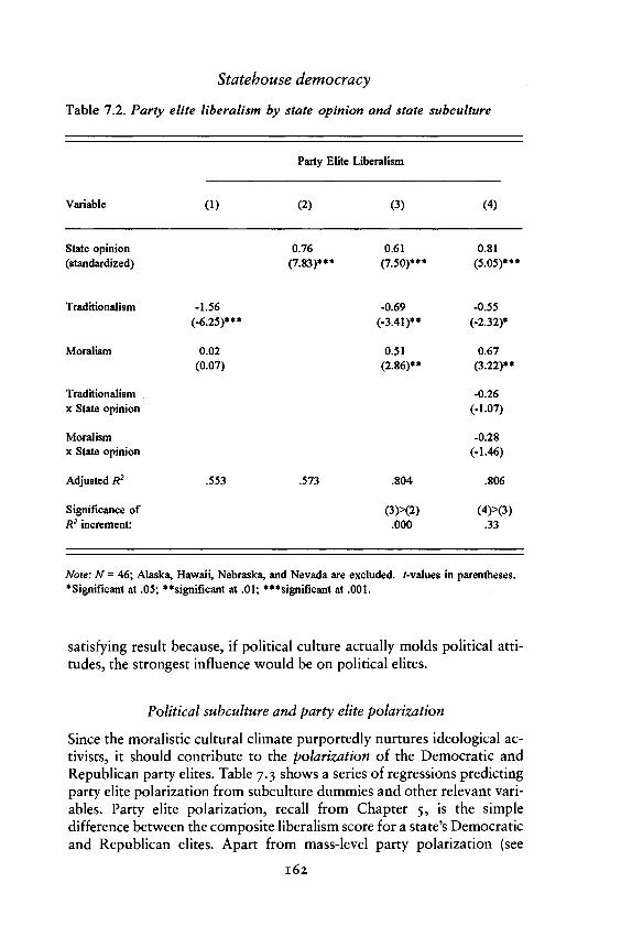
Statehouse democracy
Table 7.2. Party elite liberalism by state opinion and state subculture
Variable
State opinion(standardized)
Traditionalism
Moralism
Traditionalismx State opinion
Moralismx State opinion
Adjusted R2
Significance ofR2 increment:
(1)
-1.56(-6.25)***
0.02(0.07)
.553
Party Elite
(2)
0.76(7.83)***
.573
Liberalism
(3)
0.61(7.50)***
-0.69(-3.41)**
0.51(2.86)**
.804
(3)>(2).000
(4)
0.81(5.05)***
-0.55(-2.32)*
0.67(3.22)**
-0.26(-1.07)
-0.28(-1.46)
.806
(4)>(3).33
Note: N = 46; Alaska, Hawaii, Nebraska, and Nevada are excluded, f-values in parentheses.•Significant at .05; **significant at .01; ***significant at .001.
satisfying result because, if political culture actually molds political atti-tudes, the strongest influence would be on political elites.
Political subculture and party elite polarization
Since the moralistic cultural climate purportedly nurtures ideological ac-tivists, it should contribute to the polarization of the Democratic andRepublican party elites. Table 7.3 shows a series of regressions predictingparty elite polarization from subculture dummies and other relevant vari-ables. Party elite polarization, recall from Chapter 5, is the simpledifference between the composite liberalism score for a state's Democraticand Republican elites. Apart from mass-level party polarization (see
162

Political culture and policy
Table 7.3. Party elite polarization by state opinion and state subculture
Variable
State opinion(standardized)
Traditionalism
Moralism
Mass partypolarization(standardized)
Intercept
Adjusted R2
(1)
0.05(0.36)
0.44(3.22)**
1.41(13.83)
.202
Party
(2)
-0.02(-0.30)
-.021
Elite Polarization
(3)
-0.01(-0.17)
0.03(0.19)
0.43(2.90)**
1.42(12.19)
.184
(4)
-0.06(-0.92)
0.16(0.95)
0.36(2.56)*
0.18(2.63)*
1.40(12.83)
.285
Note: N = 46; Alaska, Hawaii, Nebraska, and Nevada are excluded, /-values in parentheses.*Significant at .05; **significant at .01; ***significant at .001.
Chapter 2), moralistic subculture is the sole variable that consistently pre-dicts party elite polarization. Thus, party elites are more liberal but alsomore ideologically polarized than in other states.
This result presents a certain irony. Earlier (Chapter 5), we noted thatseveral categorizations of states that scholars had posited to predict polar-ized parties in fact did not; but they did in each case predict party eliteliberalism. Elazar's classification is an exception to this rule. Elazar's mor-alistic states produce party elites that are more polarized but not (in theabsence of controls) noticeably more liberal. With state opinion con-trolled, however, the party elites of the moralistic states are both morepolarized and more liberal.
How can moralist party elites be more liberal and more polarized ideo-logically? Figure 7.3 presents Democratic and Republican party elite liber-alism scores as a function of state opinion, separately for each subculture.
163

Statehouse democracy
Moralistic
NDSD
IDUT
^ ^ND
UT SDID
CA
KS^NH/T ^ W A
KS NH Wl WACOCA
MT
<a£
State Opinion
Figure 7.3 Party Ideology and StateOpinion by Political Subculture. Note:Democrats above the diagonal;Republicans below.
We scale this figure like we did Figure 6.5, forcing state opinion and partyelite liberalism onto a common metric based on the assumption that,nationally, the party midpoint is uncorrelated with state opinion. Notethat parties are farther apart in moralistic states, with the key differencebeing that Democratic elites in moralistic states are unusually liberal -more liberal, that is, than their counterparts in individualistic or tradi-
164

Political culture and policy
tionalistic states with the identical degree of liberalism among the masspublic.4
Figure 7.3 also presents a hint of how the relative proximity of theparties to the electorate may vary by subculture. Presented with liberalparty elites, the electorates of moralistic states appear ideologically closerto their local Republican parties. Meanwhile, given conservative partyelites, the electorates of traditionalistic states appear closer to their localDemocratic parties. These differences suggest some subcultural variationin partisan voting - a subject that we turn to next.
Political subculture and legislative partisanship
When state party elites diverge ideologically from the preference of stateopinion, the electorate can make the ideological correction at the ballotbox. Electorates in traditionalistic states, with elites more conservativethan projected from state opinion, can correct by leaning toward theirrelatively conservative Democratic parties over their seemingly too con-servative Republican parties. Similarly, electorates in moralistic states,with elites more liberal than projected from state opinion, can correct byleaning toward their relatively liberal Republican parties over theirseemingly too liberal Democratic parties.
Table 7.4 shows a series of equations predicting Democratic legislativestrength from state opinion, party elite liberalism, and the additive andinteraction effects of the culture dummies. Column 1 shows the simpleprediction from culture alone. As expected, the traditionalistic states tendto have strongly Democratic legislatures. Moralistic states have legisla-tures that are far more Republican than average. Column 2 presents therepresentation equation without the culture dummies. Democratic legisla-tive success is greatest when state opinion is most liberal and when partyelites are most conservative. This is consistent with Downsian logic, sinceDemocrats are closer to the electorate when both parties are more conser-vative than their norm, and Republicans are closer to the electorate whenboth parties are more liberal than their norm (see Chapter 6).
Column 3 shows the result with culture dummies combined additivelywith state opinion and party elite liberalism as predictors of Democraticlegislative strength. The moralistic pro-Republican "effect" almost van-ishes, as if it is accounted for by moralistic electorates adjusting for theirseemingly overly liberal party elites. However, even with the controls, thetraditionalistic subculture still shows a positive effect on Democratic legis-
4. As an alternative, we can repeat this analysis by subdividing party elite liberalisminto scores for activists and electoral elites, as done in Chapter 5. The greater polar-ization of the parties in moralistic states is present for both groups of elites, butstronger for activist elites than for electoral elites.
165

Statehouse democracy
Table 7.4. Accounting for democratic legislative success
Variable
State opinion(standardized)
Party eliteliberalism(standardized)
Traditionalism
Moralism
Traditionalismx State opinion
Moralismx State opinion
Traditionalism xParty elite liberalism
Moralism x Partyelite liberalism
Adjusted R2
Significance ofR2 increment:
(1)
0.97(3.55)***
-0.66(2.47)*
.467
Democratic
(2)
0.79(4.44)***
-1.02(-5.75)***
.409
legislative success
(3)
0.57(3.07)**
-0.37(-1.59)
1.22(3.54)***
0.20(0.70)
.557
(3)>(2).001
(4)
1.62(4.25)***
-1.16(-2.77)**
0.54(1.65)
-0.17(0.53)
-1.38(-3.03)**
-1.31(-3.14)**
-0.08(-0.15)
1.48(3.05)**
.776
(4)>(3).000
Note: /-values in parentheses.*Significant at .05; **significant at .01; ***significant at .001.
lative strength. Traditionalism is a marker for the once one-party politicsof the southern political culture (Key, 1949).
Column 4 shows the interaction effects involving culture. These are thesubculture-to-subculture differences in the effects of state opinion andparty elite liberalism on Democratic legislative strength. Here, for the firsttime, we find strong evidence that effects of other variables depend on
166

Political culture and policy
subculture. Both traditionalistic and moralistic subcultures appear to se-verely dampen the gradient by which a state's electorate translates itsideological preferences into the partisan division of legislative seats.Effects of state opinion on Democratic legislative strength are 1.62 forindividualistic states (the base), 0.31 (or 1.62 - 1.31) for moralistic states,and 0.24 (or 1.62 - 1.38) for traditionalistic states. Meanwhile, moralism(but not traditionalism) appears to dampen the coefficient for party eliteliberalism - as if electorates in moralistic states give little regard to theirparties' ideological nuances. The party elite liberalism coefficient changesfrom -1.16 (the base, for individualistic states) to 0.32 (or -1.16 + 1.48)for a sign reversal in moralistic states. These patterns are highly significantstatistically. How do we account for them?
For traditionalistic states, the seemingly less responsive electorate maybe a by-product of the supposed elite domination of the electoral process.For moralistic states, we need a different explanation because their par-tisan legislative divisions are less responsive to both state opinion and eliteideology. Our speculation is that the seemingly sluggish electoral responsein moralistic states is actually a response to the more programmatic par-ties. With polarized parties that approximate the national party positionsideologically, minor differences in our measure of party positions shouldhave little impact on partisan voting. Party polarization, however, magni-fies the policy impact of each increment of Democratic legislative control(discussed ahead). Thus, provided with more programmatic divergentparties, electorates in moralistic states can employ a smaller partisan ad-justment to achieve a given ideological result. The statistical result is thesmaller regression coefficients in moralistic states for the effect of stateideology on legislative party strength.5
The interaction effect of moralism on the effect of party elite liberalismon Democratic legislative strength suggests that moralistic electorates ig-nore nuances of each party's ideology. This makes sense for the samereason that a low coefficient for state opinion makes sense when the par-ties are polarized. With ideologically diverse parties, electorates in moral-istic states properly respond by fine-tuning the correct electoral mix ofconservative Republicans and liberal Democrats, rather than selectively
5. It may seem counterintuitive that polarized parties produce lesser coefficients forstate opinion predicting a partisan response. Consider, however, the following hypo-thetical examples. In Set A of states, the Democratic and Republican positions are0.5 and -0.5, respectively. In Set B, the Democratic and Republican parties arefarther apart, at 1.0 and -1.0. Suppose, in each set, the state electorates chose thepartisan mix that matches its mean ideological preference on the same scale. A stateat -0.5 would choose all Republicans if in Set A but only 75 percent Republicans ifin Set B (0.75 x (-1) + 0.25 x (+1) = -0.5. Similarly, a state at +0.5 would choose allDemocrats if in Set A but only 75 percent Democrats if in Set B. For Set A, the slopeis 2.0, or 1.0 - (-1.0). For Set B, the slope is 1.5, or 0.75 - (-0.75).
167

Statehouse democracy
rewarding parties for their ideological moderation, as electorates in indi-vidualistic and traditionalistic states can do.
Political subculture and legislative liberalism
We measure legislative liberalism as the combination of Democratic andRepublican party elite liberalism, rescaled so that the two party elites areweighted in accordance with their legislative strength. Since legislativeliberalism is defined in terms of party elite liberalism and Democraticlegislative strength, there is little to be gained by pursuing the direct effectsof subculture on legislative liberalism. Instead, we examine how subcul-ture might alter the net (direct plus indirect) effect of state opinion onlegislative liberalism. Following our usual procedure, we examine first thesimple additive models and then the conditional impact of state culture onthe net state opinion-legislative liberalism relationship. Table 7.5 showsthe details.
Column 1 shows the simple differences in legislative liberalism acrosssubcultures. Without controls, there is not much of a relationship, but wedo see the greater conservatism among the legislators of traditionalisticstates. Column 2 shows the strong (r = .79) bivariate relationship betweenstate opinion and legislative ideology. Column 3 shows the joint additiveeffects of culture and state opinion. With interaction effects not yet in-cluded, the additive effects of culture on legislative ideology are not signif-icant.
Column 4 adds the interaction effects. The net responsiveness of legisla-tive liberalism to state opinion is very strong (1.22) in individualisticstates, slightly (and insignificantly) less (0.94 = 1.22 - 0.28) in the moralis-tic states, and almost invisible (0.34 = 1.22 - 0.88) states. Thus, if wegauge the quality of representation by the responsiveness of legislativepreferences to opinion in the state, the traditionalistic subculture gets lowmarks.
Traditionalism by itself, however, does not seem to breed legislativeconservatism. An ideologically middle-of-the-road state would haveabout the same kind of legislature ideologically, whether the state em-braced the traditionalist or individualist culture. We also see that with theinteraction terms included, a significant, positive coefficient emerges formoralistic states. A moralistic subculture appears to provide the state witha more liberal legislature than otherwise, even after the electoral process isallowed to do its work.
The policy equation
The story does not end with the determination of the ideological leaningsof state legislatures. State policies are not an exact function of the legisla-
168

Political culture and policy
Table 7.5. State opinion, state subculture, and legislative liberalism
Variable
State opinion(standardized)
Traditionalism
Moralism
Traditionalismx State opinion
Moralismx State opinion
Adjusted R2
Significance ofR2 increment:
(1)
0.82(9.62)***
.670
Legislative liberalism
(2)
0.90(8.67)***
0.33(1.27)
0.37(1.64)
.676
(2)>(1).26
(3)
1.22(6.39)***
0.24(.83)
0.63(2.56)*
-0.88(-3.03)**
-0.28(-1.20)
.725
(3)>(2).014
Note: N = 46; Alaska, Hawaii, Nebraska, and Nevada are excluded, /-values in parentheses.•Significant at .05; **significant at .01; ***significant at .001.
tors' collective preferences. The partisan division of the legislature canmake a difference. Also, legislatures sometimes allow public opinion tooverride their own preferences (Miller and Stokes, 1963). Our final statis-tical task is to see how these processes are affected by subculture.
Table 7.1 showed the additive and interaction effects involving stateopinion and political subculture as predictors of state policy liberalism.Table y.6 shows the policy equations that also include additive and inter-action effects involving Democratic legislative strength and legislative lib-eralism. We focus mainly on the "best" equation shown in Column 3,which includes terms for the interactions of culture with state opinion andDemocratic legislative strength but excludes those involving legislativeliberalism. Several features of the results warrant attention.
First, note the additive moralistic effect in the conditional models of
169

Statehouse democracy
Table 7.6. Accounting for state policy liberalism
Variable
State opinion(standardized)
Legislative liberalism(standardized)
Democraticlegislative strength(standardized)
Traditionalism
Moralism
Traditionalx State opinion
Moralismx State opinion
(1)
0.44(3.59)***
0.48(3.88)***
-0.32(_4.48)***
Traditionalism x Democraticlegislative strength
Moralism x Democraticlegislative strength
Traditionalism xLegislative liberalism
Moralism xLegislative liberalism
State policy liberalism
(2)
0.40(3.08)**
0.36(2.72)**
-0.09(-0.41)
-0.56(-2.29)*
0.09(0.47)
(3)
1.14(4.47)***
0.14(0.93)
-0.44(2.28)*
-0.18(-0.71)
1.08(2.92)**
-0.73(-2.60)*
-0.88(-3.23)**
0.37(1.57)
0.95(2-65)*
(4)
1.11(2.77)**
0.16(0.51)
-0.44(-2.15)*
-0.25(-0.42)
1.00(2.51)*
-0.63(-1.38)
-0.88(-2.01)
0.39(1.55)
0.87(2.00)
-0.22(-0.46)
0.04(0.11)
Adjusted R2
Significance ofR2 increment:
.799 .819 .846 .839
.047 .040 .809
Note: /-values in parentlieses.•Significant at .05; **significant at .01; ***significant at .001.
I7O

Political culture and policy
Columns 3 and 4. Even apart from legislative liberalism, Democratic legis-lative strength, and state opinion, something about the moralistic culturemakes moralistic states enact policies that are far more liberal than inother states. For a middle-of-the-road state (at zero - the national mean onstate opinion and Democratic legislative strength), a moralistic (instead ofindividualistic) culture is worth about a 1.08 standard deviation incre-ment in policy liberalism. This is the residual effect of the moralistic sub-culture apart from the direct working of the electoral process. No morethan a trace (-0.18) of a mirror-image "conservative" policy effect ap-pears for the traditionalistic subculture.
Second, in the full model (Column 4, see also Column 3), the combinedadditive and interactive effects of legislative liberalism become nonsignifi-cant and virtually nonexistent. The strong effect of state legislative liberal-ism seen when culture is absent from the model gets absorbed by cultureand its interactions. Quite arguably this result could be no more than anadverse response of the data to multicolinearity. But a possibility thatcannot be ruled out is that what appears to be evidence of legislaturesresponding to their own preferences could really be the by-product ofpolitical culture.
Third, especially, for the equation reported in Column 3, we observe amajor interaction effect involving moralism and Democratic legislativestrength. Whereas in individualistic (and to a lesser degree traditionalistic)states the sign for Democratic legislative strength is negative, for moralis-tic states the sign is clearly positive (0.51 = -0.44 + 0.95). In individualisticstates where a more politically pragmatic politics reigns, Democratic leg-islators trim to the right and Republicans trim to the left when makingstate policy. In fact, working through the equations suggests that partiesovercompensate, so that the best way to enact liberal policies in an indi-vidualist state might be to elect Republicans, and the best way to enactconservative policies might be to elect Democrats. But in moralistic stateswhere parties are supposedly more programmatic and clearly more polar-ized in ideological tone, partisanship accentuates policy differences. Inmoralistic states, the best way to enact liberal policies would clearly be toelect programmatic Democrats, and the best way to enact conservativepolicies would clearly be to elect programmatic Republicans.
The variation in the functioning of legislative partisanship in the policyprocess can be seen dramatically from Figure 7.4. Here, the simple cor-relation between (unstandardized) Democratic legislative strength andstate policy liberalism is shown separately for the three subcultures. Fortraditionalistic states, the legislative strength-policy correlation is actu-ally somewhat negative (-.32), with Democratic legislatures manufactur-ing the most conservative policies. For individualistic states, thecorrelation is positive but slim (.37). But for moralistic states, a sharp .89
171

Statehouse democracy
1i
2 -
1 -
o -
-1 -
-2 "
NY
Individualistic
P A D E C ^OH
IL
WY M 0
IN
MA
MDRl
Democratic Legislative Strength
Figure 7.4 Policy Liberalism andDemocratic Legislative Strength byPolitical Subculture
correlation exists, as if policy liberalism is almost solely a direct functionof Democratic legislative strength.
This last result might suggest that the moralistic subculture enhancesresponsiveness of policy to public opinion. But consider the fourth andperhaps most important observation to be made from Table 7.6. Apartfrom all legislative responses we have been considering, the direct effect ofstate opinion is strongly conditioned by political culture. From Column 3,for the reference base of individualistic states, the direct effect of opinionon policy is a major coefficient of 1.14. Meanwhile, the direct effects of
172

Political culture and policy
public opinion in the other two cultures are negligible: only 0.26 (1.14 —0.88) in moralistic states and only 0.41 (1.14 - 0.73) in traditionalisticstates. State legislatures are much less responsive to state opinion in themoralistic and traditionalistic states.
The startlingly large differences in the coefficients for moralistic andindividualistic states can be attributed to the difference between pragma-tic politicians in individualistic states and the programmatic politicians inmoralistic states. In moralistic states, the relative partisan division of legis-latures has important policy consequences, while legislatures are less re-sponsive to the direct input of public opinion. In individualistic states, theparty division has less easily discernible policy consequences, but thepragmatic legislatures respond strongly to state opinion.
Summary: Three state subcultures
Let us summarize the features of democratic representation, as it variesacross the three subcultures. As a statistical guide, Figure 7.5 summarizesthe representative processes across the three subcultures in terms of sepa-rate causal models. The continuous variables are measured in units thatare standardized at the national level rather than the subculture level, thusmaking the coefficients comparable across subcultures.
The traditionalistic subculture, representing mainly southern states,presents few surprises. For traditionalistic states, most coefficients aremuted versions of what is found when all states are considered together.The exception is a strong negative coefficient from party elite liberalism toDemocratic legislative strength. This coefficient represents the strong sen-sitivity to parties' ideological nuance on the part of southern electorates.Overall, the degree of representation is relatively low in the traditionalisticsubculture.
The comparison between the moralistic culture and the individualisticculture is particularly interesting. For individualistic states, the pattern ofcoefficients presents a hyper version of the model when all states are con-sidered together. For individualistic states, we can paint a portrait of prag-matic democratic politics, as if politicians respond to public opinion outof a desire to get and stay elected: Democratic legislative strength is astrong positive function of mass liberalism and a strong negative functionof the liberalism of party positions. Due to electoral considerations, legis-latures push policy toward the center, away from the dominant party'sideological beliefs, and respond strongly to state opinion in anticipationof electoral sanctions.
For moralistic states, the coefficients portray a system where ideologicalparties play a major role: With ideologically distinct parties, a given level
173

Statehouse democracy
0.23
MoralisticStates(n-17)
OpinionLiberalism
i-Party EliteLiberalism
0.31
0.53 0.32
1.03
DemocraticLegislative Strength
I 0.83
LegislativeLiberalism
Policy
Uberalism
1.11
IndividualisticStates(n = 13)
Opinion 1.62
Uberalism
0.81 -1.15.
Party Elite 1.07Liberalism
DemocraticLegislative Strength
I 0.56
Legislative / 0.16Liberalism
Policy
Liberalism
0.48
Tradrtionalistic ,.,States(n = 16)
Opinion 0.24
Party EliteLiberalism
DemocraticLegislative Strength
0.53 -1.23^
0.70
I 0.33
LegislativeLiberalism
Policy
Uberalism
Figure 7.5 Variations in the Policy Model by Political Culture
of change in the party division in the legislature has larger policy conse-quences. State electorates need only move in modest partisan incrementsto achieve noticeable policy changes.
Is either the pragmatic individualistic system or the responsible partiesmoralistic system noticeably "better" from the standpoint of policy repre-sentation? Based on our information, we cannot choose a winner. The netslope predicting policy from opinion is slightly larger in individualisticstates, but not significantly so. In any case, opinion and policy are mea-sured in different metrics, so we possess no direct knowledge of the idealslope for comparison. Only with the same, correct, metric for opinion and
174

Political culture and policy
policy could we assess whether any of the opinion-policy slopes are toostrong (hyper-representation) or too weak (hyporepresentation).6
CONCLUSIONSIn this chapter, we have applied Elazar's categorization of the states intothree subcultures to the task of differentiating among styles of representa-tion. Our results offer strong support - sometimes startlingly strongsupport - for Elazar's formulation. In almost all instances where we findinteraction effects or additive effects involving the subculture categories,the results are consistent with what we would expect from Elazar's discus-sion. Similarly, in almost all instances where an additive or interactioneffect is posited, one is found. Due to the impressionistic origin of Elazar'stypology, our conclusions must include a note of ambiguity regarding itsexact contribution to the study of representation. Elazar based his classifi-cations on a host of variables. Although the main defining characteristicclearly was immigration flows, the contemporary style of representationalso swayed his classification decisions. States were described as tradi-tionalistic in part because their elites tended to ignore public opinion.States were described as individualistic in part because their politicianswere pragmatic. States were described as moralistic in part because theirpoliticians tended to impose their version of the public interest on theircitizenries. The contribution of Elazar's categories to the study of repre-sentation may not be "causal" in the usual sense. Culture, as Elazardefines it, may not be a cause of representational variation. Instead, per-haps Elazar's categories should be considered as the defining characteris-tics of different styles of representation. If so, our usage (and many others)of Elazar's categories may be more of a validation exercise than a positingand testing of causal relations.
This observation is not a criticism of Elazar's formulation. It is more ofa comment on the overriding breadth of Elazar's conceptualization. Per-haps it took no great insight to classify the southern states and some oftheir neighbors as traditionalistic states where cultural expectations en-hance the insulation of the political elites from their masses. More re-markable is how the distinction between moralistic and individualisticstates separates two different modes of representation. The individualisticstates present the archetypal models of Downsian pragmatic politics asdescribed in Chapters 5 and 6. Moralistic states present an importantvariation, where party positions are more distinct and offer greater predic-
6. We could also compare the net fits of the regression lines in the different subcultures.These correlation coefficients are a similar .85 and .84 for moralistic and individu-alistic subcultures. Although these numbers provide no grounds for choosing a win-ner, they do beat the slightly lesser .66 found for traditionalistic subcultures.
175

Statehouse democracy
tion of what politicians do in office. Thus, Elazar's categories presentmore than a theoretical distinction among styles of representation. Hisclassifications enable the spotlight to be pointed at different states withreal variation in how the game of politics is played. That is an importantcontribution.
176

8Partisanship, ideology, and state elections
Among state political analysts, a common pastime is classifying the statesaccording to their degree of Republican or Democratic partisanship. Themost frequently cited is Ranney's (1976) classic measure of interpartycompetition. The Ranney index is a combination of the two parties' rela-tive legislative strength and the two-party vote for governor. Used as adirectional measure, the Ranney index arrays the states on a continuumfrom safely Democratic to safely Republican. "Folded," the index mea-sures the distinction between "competitive" states and "one-party" states.Others, notably David (1972), have developed indexes of state partisan-ship based on the vote for a wide variety of state offices. The rationale forclassifying the states on the basis of partisanship is the measurement ofmeaningful differences in the two parties' relative chances of winningelections. Presumably, some states almost always elect Democrats andothers almost always elect Republicans, with others in the middle enjoy-ing the presumed ideal condition of "competitive" elections.
To what extent are statewide election outcomes determined by statelevels of Democratic versus Republican partisanship? Our measure ofstate party identification can help to answer this question. In Chapter 6,we saw that the correlation between state party identification and legisla-tive partisanship was a quite high .87. This strong correlation was to beexpected, because the measure of legislative partisanship is the net balanceof all legislative races, averaged for each chamber over eight electionyears.
But when we turn to the vote for major state-level offices (governor orU.S. senator) or for president, state partisanship is a less certain electoralpredictor. For instance, by all historically based measures of party com-petition, as well as our measure of state partisanship, southern states aredecidedly Democratic. But as everybody knows, southern states are nolonger Democratic at the presidential level and quite often vote Republi-can for major state offices. Meanwhile, traditionally Republican states
177

Statehouse democracy
have been the source of many Democratic electoral victories. The bestcontemporary example is the traditionally Republican state of NorthDakota. In the late 1980s, "Republican" North Dakota was the only statewith a Democratic governor, two Democratic U.S. senators, and a solidlyDemocratic U.S. House delegation (admittedly, with an N of 1). NorthDakota's clustering of major offices in the hands of one party is rareenough, but for the clustering to favor the party seemingly disfavored bythe state's underlying partisanship presents a particularly strong anomaly.Given recently observable levels of partisan unpredictability in state elec-tions, it would seem that (to borrow a sports cliche) in any given state,each party has a solid chance of winning major state office. The reason,we will see, is that state electoral outcomes depend on the relativestrengths of the competing candidates as well as the strengths of the stateparties.
This chapter explores state-level elections. We examine state-level vot-ing for three offices: governor, U.S. senator, and U.S. president. We set ourfocus on the contribution of the two central variables of this project - stateelectorates' mean levels of party identification and ideological identifica-tion.
In order to explore the micro-/macrolevel electoral connection in thestates, we also exploit CBS/NYT Election Day exit polls. Between 1982and 1988, CBS/NYT conducted 73 separate state-level exit polls in whichrespondent ideological and partisan identifications were asked. Stateswere selected on the basis of general interest in their senatorial and guber-natorial contests, so that, when applicable, vote choices for governor andU.S. senator were ascertained. For 1984 and 1988, these exit poll surveysascertained the respondents' presidential votes as well. Since each stateexit poll includes about a thousand respondents, such polls provide thebest measure of mean partisanship and ideology for voters in specific stateelections.
As a guide for our investigation of state-level election outcomes, weborrow some old but useful conceptual language that was introduced bythe American Voter authors in their second book together, Elections andthe Political Order (Campbell, Converse, Miller, and Stokes, 1966). InElections and the Political Order (hereafter referred to as EPO),Campbell et al. presented election outcomes as a composition of the "nor-mal vote" for the particular constituency (states in our investigation) plusdeviations from the normal vote, which they termed "short-term partisanforces" (Campbell, 1966; Converse, 1966).
The "normal vote" is the two-party vote division that would resultfrom an election in which the "balance of partisan forces are equal" (Con-verse, 1966). Roughly speaking, this would be the neutral electoral out-come in which Democratic and Republican partisans defect at equal rates
178

Partisanship, ideology, and elections
and voters who are Independent split their votes 50-50 between Republi-can and Democratic candidates. In EPO terminology, deviations from thenormal vote are due to "short-term partisan forces." Writing a quartercentury ago, Campbell (1966) posited "short-term" forces to be strongestin "high stimulus" national presidential elections, when turnout, interest,and information peak. Campbell theorized that short-term forces wouldbe weak for nonpresidential offices - particularly when the election isconducted at midterm.
As Campbell saw it, elections below the presidential level were "lowstimulus" affairs that were decided by little more than partisans voting fortheir party. (The one clear exception would be when election outcomes areinfluenced by the short-term forces of higher-level elections conducted atthe same time - what are usually termed "coattail" effects.) This ratherstatic view of subpresidential election outcomes, however, was not basedon any analysis of actual election outcomes, at least none that Campbell etal. presented to the reader. It was instead an inference from individual-level survey data. The survey data available to Campbell et al. showed astrongly partisan U.S. electorate and a relatively uninvolved and unin-formed U.S. electorate, particularly when it came to elections below thepresidential level. (See Stokes and Miller, 1966, in addition to the pre-viously mentioned EPO references.) It is easy to see how the nationalelectorate, considered from the perspective of the 1950s through themid-1960s would lead to the view that elections below the presidentiallevel were basically predictable partisan affairs. Indeed, based on a casualreading of the political science literature of this earlier era, one mightthink that the way to forecast an election for U.S. senator or governorwould be simply to consult one's favorite index of party competition in thestates and extrapolate the election outcome from the states' partisan na-tures.
To political scientists steeped in the voting literature of the 1970s,1980s, and 1990s, the EPO expectation of weak short-term forces in elec-tions below the presidential level appears curiously in error. The literatureon congressional elections, which once emphasized constituency partisan-ship, now emphasizes the candidates and their campaigns (e.g., Mann,1978; Jacobson, 1990; Erikson and Wright, 1993). This new emphasis hasspread from U.S. House campaigns to include statewide U.S. Senate elec-tions as well (e.g., Wright and Berkman, 1986; Abramowitz, 1988; Squire,1989). Even gubernatorial elections are being discovered (Kenney, 1983;Kenney and Rice, 1983; Patterson and Caldiera, 1983; Tompkins, 1984;Holbrook-Provow, 1987; see also Wright, 1974). Below the presidentiallevel, campaign stimuli - and not just constituency partisanship - matter.So, let us take a fresh statistical look at state-level election results. Ourmajor concern is the state vote for governor and U.S. senator. We start,
179
Statehouse democracy
however, with a more familiar data set - state voting patterns for the officeof president.
STATE VOTING IN PRESIDENTIAL ELECTIONS
It is widely known that national presidential election outcomes cannot beprojected from the national distribution of party identification. Given theusual Democratic edge in party identification, the normal vote predictionfor national elections is a margin of about 54 percent Democratic and 46percent Republican. This prediction of a 54-46 Democratic edge approx-imates the national average vote division in recent House elections. Recentpresidential elections, however, have decidedly favored the RepublicanParty. Table 8.1 presents the evidence. Over 11 elections, the record is 7Republican victories and 4 Democratic victories. The mean national votedivision for president over this span is 52.5 percent Republican, 47.5percent Democratic. Clearly, the usual division of Democrats and Re-publicans is a poor expectation for national presidential election out-comes. Instead, let us substitute the mean 1952-92 presidential votedivision (47.5 percent Democratic) as the best estimate of the normalnational presidential vote. We can more reasonably estimate short-termforces of presidential campaigns as departures from this electorally basednorm than as departures from the 54 percent Democratic normal vote.
Note that the standard deviation of the national vote is a relatively large6.5 percentage points. This standard deviation serves as a rough index ofthe general magnitude of national short-term forces for president, 1952-92. As a measure of short-term forces, the 6.5 standard deviation reflects asampling distribution in which outlier landslide elections such as 1964(Johnson vs. Gold water) and 1972 (McGovern vs. Nixon) are almost twostandard deviations from the mean. Later we will use this 6.5 estimate ofshort-term forces in national presidential elections as a standard of com-parison for our estimates of the magnitude of short-term forces in senateand gubernatorial elections.1
The macro-level: Party, ideology, and the presidential vote
In this section, we bring to bear some unusual resources to explore state-level differences in presidential voting. To what extent does state variation
1. Of course, other methods could be used to estimate the national-level short-termforces. We could, for instance, control for a linear time trend, which would lower theestimate of short-term forces. We could alternatively assume as correct the baselineof a 54 percent Democratic normal vote. Deviations of the presidential vote fromthis baseline would of course increase the estimate of the short-term forces. If we doan ordinary Mest of the hypothesis that the mean outcome is 54.0 percent Democra-tic, using the 11-year distribution of the two-party vote, the hypothesis can be re-jected at the .05 level.
180

Partisanship, ideology, and elections
Table 8.1. Democratic presidential vote, 1952-92
State Vote
45.043.249.457.847.735.950.142.938.944.851.8
11.28.65.9
13.27.16.96.18.15.85.56.2
NationalYear Vote Mean S. D.
1952 44.61956 42.21960 50.11964 61.31968 49.61972 38.21976 51.11980 44.41984 40.81988 46.21992 53.5
Mean 47.5 46.2 7.7S. D. 6.5
Note: Based on 48 contiguous states. All computations in terms of the Democratic share of thetwo-party vote.
in presidential voting depend on state-level party identification and state-level ideological identification?
Table 8.1 summarizes the univariate statistics of not only national-levelbut also state-level presidential voting. Of particular interest is the state-level standard deviation for each election year. The median value of thisstatistic is 7.7 percent, or about the same as the national-level standarddeviation. We can summarize this comparison in the following way. Topredict how a state will vote in a presidential election, it is virtually of thesame importance to know which state is referenced as to know the partic-ular election year.
It has long been recognized that state-level presidential outcomes reflectstate differences in partisanship and ideology. In the mid-1980s,Rabinowitz, Gurian, and McDonald (1984) presented an innovative fac-tor analysis of state presidential voting. They found two factors, whichthey labeled partisanship and ideology. The partisan factor strongly corre-lated with state partisanship in voting below the presidential level. Theideological factor strongly correlated with ideological voting by the states'
181

Statehouse democracy
congressional delegations. Rabinowitz et al. found a growing importanceof the ideological factor at the expense of the partisan factor.
Our data show a similar pattern: State-level voting in recent presidentialelections is more a function of state ideological identification than of stateparty identification. In past elections, however, state party identificationused to dominate. Table 8.2 presents the regressions of presidential votingin specific elections, 1952-92, on our CBS/NYT measures of state ideol-ogy and partisanship. Note the growing importance of ideology at theexpense of partisanship. In terms of our survey measures obtained overtwo decades later, partisanship determined the two Eisenhower elections(1952, 1956) at the expense of ideology. Ideology did not become impor-tant until the contests of 1964 (Johnson-Goldwater) and 1972 (Nixon-McGovern). In 1976, partisanship rebounded for the Carter-Ford con-test. The 1984 and 1988 contests saw a strong return of ideological identi-fication as a determinant of the state-level presidential vote.
All this conforms with most observers' interpretations of recent presi-dential elections. One might even think that the task is complete - thatthere is very little more beyond Table 8.2 that can be said statisticallyabout state presidential voting. But one interesting puzzle remains: Wehave seen that in recent presidential elections, ideology has dominatedpartisanship as a predictor of state-level voting. Yet when we study indi-vidual voters instead of states, voter partisanship is a decisively betterpredictor of presidential choice than is voter ideology. What accounts forthis discrepancy? We will spend some effort trying to solve this puzzle.Finding a solution requires that we identify the linkages in the seeminglycontradictory macro-/microlevel relationships.
1984 and 1988 exit poll data
To better understand the micro/macrolevel connection for presidentialvoting at the state level, we simulated state election outcomes from theElection Day state exit polls conducted by CBS News/NYT on electionday in 1984 and 1988- 18 in 1984 and 24 in 1988. Each exit poll containsfrom 652 to 2,778 voters, each interviewed as they left their polling place.Given exit poll methodology, it is essential that the data be "weighted"rather than used in raw form. The weights were furnished by CBS/NYT.Among other considerations, each state's Bush and Dukakis voters arereweighted in the necessary fashion to generate the correct proportions ofBush and Dukakis voters in the voting electorate. In other words, theweighted marginals for the state samples equal the actual vote. This is astrong convenience, as it allows one to make forecasts of state voting fromsample distributions without worrying about adjusting for sampling errorin the dependent variable.
182

Partisanship, ideology, and elections
Table 8.2. Predicting the state presidential vote from state partisanshipand ideology
47 States 36 Nonsouthern states
Partisanship Ideology Partisanship Ideology
b Beta b Beta Adjusted b Beta b Beta AdjustedR2 R2
1952
1956
1960
1964
1968
1972
1976
1980
1984
1988
1992
0.62** .63
0.45** .60
0.36** .68
-0.27**-.23
0.30** .48
-0.08 -.14
0.43** .80
0.49** .70
0.20** .41
0.09* .19
0.18** .34
-0.26
-0.41**
0.14
1.17**
0.43**
0.70**
0.10
0.41**
0.52**
0.51**
0.64**
-.17
-.34
.17
.64
.43
.73
.11
.37
.66
.68
.76
.384
.420
.484
.413
.424
.518
.646
.662
.632
.496
.718
0.37*
0.30**
0.15
0.12
0.20
0.07
0.35**
0.38**
0.23**
0.19*
0.18*
.61
.62
.28
.19
.28*
.11
.68
.48
.36
.35
.28
0.14
-0.15
0.40**
0.60**
0.61**
0.51**
0.18*
0.56**
0.51**
0.38**
0.62**
.16
-.22
.54
.67
.61
.61
.25
.51
.58
.50
.69
.470
.264
.493
.577
.590
.410
.662
.698
.640
.508
.725
Note: N=47. Nevada, Alaska, and Hawaii are omitted.•Significant at .05 level; **significant at .01 level.
To begin, we explore a model that forecasts exit poll presidential votessolely from trichotomous partisanship and ideology. With a dichotomousdependent variable (Republican vote = o; Democratic vote = l), the appro-priate multivariate technology is probit analysis rather than our usualOLS regression. These probit equations, for 1984 and 1988, are shown inTable 8.3, Columns 1 and 4. In both contests, partisanship is clearly thestronger of the two vote predictors, but with ideology a respectable sec-
183

Table 8.3. Probit equation of presidential vote in 1984 and 1988CBS/NYT exit polls
Partyidentification
Ideologicalidentification
State partyideological midpoint
Intercept
ALCACTFLILINIAMDMAMIMNMSNVNHNJNMNYNCOHORPATXVTWA
wvWI
Estimated R2
1984
(N = 26,638)
(1) (2)
1.02** 1.04**(84.0) (84.2)
0.52** 0.51**(39.0) (37.4)
-0.30**(-30.2)
-0.52**-0.29**
-0.28**
-0.09*
-0.30**-0.26**0.01
-0.54**
-0.41**-0.36**
-0.25**-0.58**-0.40**-0.17**-0.18**-0.52**-0.16**
-0.31**0.12**
.529 .540
(3)
1.04**(84.2)
0.51**(37.4)
0.12**(13.6)
-0.36**(-32.8)
.536
(A
(4)
1.03**(90.4)
0.67**(48.4)
-0.06**(-6.2)
.572
1988
r= 30,414)
(5)
1.05**(90.1)
0.66**(47.3)
0.04-0.07-0.28**-0.01-0.23**0.29**
-0.20**-0.08-0.030.14**
-0.43**
-0.13**-0.15**0.04
-0.26**-0.15**0.19**
-0.06-0.19**0.12*0.14**
.578
(6)
1.04**(90.2)
0.66**(47.3)
0.11**(13.1)
-0.10**(-10.2)
.582
Note: t-values in parentheses.•Significant at .05; **significant at .01.

Partisanship, ideology, and elections
ond, especially in 1988. The two intercepts reflect the tilt of the voteamong voters at "zero" - that is, among moderate Independents. Bothintercepts are negative, reflecting the Republican short-term forces of thetwo presidential contests.
To convert these equations into state-level predictions, we first converteach voter's probit prediction into the probability of a Democratic vote.Then, we averaged these probabilities for each state's (weighted) exit pollrespondents to obtain state-level percentage point predictions.
The result of our simulation exercise is a set of state projections basedon the individual-level equations and the marginal distributions on theindependent variables (partisanship, ideology) in the CBS/NYT exit polls.These estimates represent a forecast for the state assuming (1) the(weighted) marginal distributions of party and ideological identificationfor the state in the 1984 and 1988 exit polls, plus (2) the probit coefficientsfor the effects of party and ideological identification on presidential votingfound in the 1984 and 1988 exit polls.
How well these projections predict the actual 1984 and 1988 vote canbe seen in Figure 8.1. The remarkable aspect of the two graphs is thedegree to which the state presidential projections are off the mark. Theforecasts correlate at only .58 (1984) and .70 (1988) with the state vote.Under the circumstances, these are not strong correlations. Our post hocsimulations of the state vote from state-level marginal distributions ofpartisanship and ideology cannot even explain half the variance in statevoting.
Our exit poll data contain sufficiently large state samples to allow us toestimate the effect of state context as an additional source of presidentialvoting. Columns 2 and 5 of Table 8.3 show the individual-level equationswith state effects added. State effects reflect state-to-state differences inthe intercept of the equation and contribute only modestly to the predic-tion of individual votes, but they are of major importance at the statelevel. By definition, each state's observed partisan and ideological com-position plus the state effect fully accounts for the state presidential vote.2
In part, state effects can reflect the influence of omitted individual-levelvariables that change from state to state. More important, state effectsrepresent the contextual effects of residence in the state. But what arethese contextual effects? Inspection of the 1984 and 1988 state coeffi-cients reveals that positive (pro-Democratic) coefficients tend to cluster inliberal and Republican states - as if state Democratic strength retardsDemocratic voting while state liberalism encourages Democratic voting,
2. Technically speaking, the sum of the products of the state mean and coefficient foreach variable plus the intercept exactly predicts the state mean score on the underly-ing probit model. The state vote is a modestly curvilinear function of the underlyingmean score.
185

Statehouse democracy
S.
50"
45
40"
35"
30"
/
NH
IA
IL0*
" M I /
TX
MN
PA
OHNJ
ALMS
MA
N Y /
NC
30 35 40 45 50
Predicted Percent Democratic,1984
I
55"
50"
45"
40" INFL
IAMf
ORWlWA
VT IL PA,CA 140
/
NJ
^OHTX
NC
MS
j /^MA
NY /
/ MONM
40 45 50 55
Predicted Percent Democratic,
1988
Figure 8.1 Simulating Presidential Vote from Exit Poll Party Identification andIdeology
186

Partisanship, ideology, and elections
each over and above what the individual's partisanship and ideologywould indicate.3
From a purely statistical standpoint, this result properly accounts forwhy the role of ideology appears exaggerated and the role of partisanshipappears muted in state-level presidential election returns. The macrolevelregression coefficients for partisanship and ideology reflect both theindividual-level effects and state-level contextual effects. Our next task isto make theoretical sense of the state-level contextual effects on the presi-dential vote.
State partisanship in presidential elections
The seeming unimportance of state partisanship in presidential electionshas its roots in the fact that state partisanship is shaped by state as well asnational politics. In Chapter 6, we saw that state partisanship is shaped bythe electorate's own ideological leanings but also by its reaction to theideological tilt of the state's party elites. Where the party elite midpoint isto the left of the electorate's mean position, the electorate will tilt towardthe Republicans in its party identification. Where the midpoint is to theright of the electorate's, the electorate will tilt toward the Democrats. Inthis way, state partisanship is an indicator of whether the parties collec-tively are too liberal or too conservative for their state-level constituen-cies.
Theoretically, to a rational electorate this "state politics" component ofpartisanship would be of little relevance to presidential voting, but em-pirically, its actual importance depends on the degree of "stickiness" ofstate partisanship when people vote for president. At one possible ex-treme, the state politics component could "irrationally" govern how stateelectorates vote for president, with citizens unable to shake the influenceof those aspects of their partisanship that are irrelevant to the voting taskat hand. At the other extreme, we can imagine state electorates respond-ing to the task of choosing a president as if that portion of their partisan-ship induced by state politics did not matter.
We will sho*w that the reality of presidential voting is closer to the latterof these two extremes. Two relatively liberal parties make state electoratesmore Republican than otherwise, and two relatively conservative partiesmake state electorates more Democratic than otherwise. The "extra"Democrats or Republicans recruited by the ideological division of stateparties are the most likely to defect in presidential politics. Restated, state
3. The state coefficients correlate at -.61 (1984) and -.49 (1988) with state partisan-ship and .49 (1984) and .48 (1988) with state ideology. The comparable correlationswith exit poll partisanship and ideology are -.11 (1984) and -.22 (1988) for par-tisanship and .58 (1984) and .71 (1988) for ideology.
187

Statehouse democracy
party ideology exerts an independent effect on presidential voting. Con-trolling for party identification, party elite liberalism "causes" Democra-tic presidential voting.
Figure 8.2 demonstrates the effect of party elite ideology on state presi-dential voting. It shows the relationship between the state ideological mid-point on the one hand and the 1984 and 1988 state coefficients (fromTable 8.3) on the other. As presented in Chapter 5, net party elite ideologyis a standardized measure, calibrated as the average (or midpoint) of thetwo parties' scores on a composite index of four components - based onthe ideologies of the parties' congressional candidates, state legislators,national convention delegates, and county chairs.
As Figure 8.2 illustrates, the party midpoint correlates with the stateprobit coefficients at .81 in 1984 and .73 in 1988. With a bit over half ofthe variance in the state coefficients explained by state party ideology, it isno overstatement to claim that state party ideology accounts for most ofthe variance in recent state-level presidential voting that cannot be ac-counted for by state partisanship and ideology.
We can also insert state party ideology directly into the exit poll equa-tions, as a contextual variable in place of the state dummy variables. Theseequations are shown in Table 8.3, Columns 3 and 6. Simulations of thestate vote from these equations offer considerable improvement in pre-dicting the vote over simulations from state partisanship and ideologyalone from Figure 8.2. Figure 8.3 shows that our new simulations basedon exit poll respondents' partisanship and ideology, plus party elite ideol-ogy, correlate impressively - at .83 (1984) and .85 (1988) -with the actualstate vote. The peculiar contribution of party elite ideology solves theearlier puzzle of why it seemed there existed state-level contextual effectsthat retarded Democratic voting in Democratic states but encouragedDemocratic voting in liberal states. These are spurious patterns, generatedby the correlations of state partisanship and ideology with the ideologicaltendencies of the state parties. For reasons we have explored, liberal stateparties are associated positively with liberal electorates but negativelywith Democratic electorates. Once we control for state party ideology, nocorrelation remains between either state partisanship or state ideologyand the state coefficients.4
For a broader demonstration of the role of state party ideology in pre-dicting state presidential voting, let us return to the 46-state analysis andour familiar CBS/NYT aggregations of state partisanship and ideology for
4. With state party ideology included in the model, all evidence of a partisan or ideolog-ical contextual effect vanishes. For instance, if mean state partisanship and meanstate ideology are added to the individual-level probit equations that include partyideology, neither mean partisanship nor mean ideology achieves statisticalsignificance - even with the many thousands of cases.
188

Partisanship, ideology, and elections
s °
E
.ffic
ie
13
Pro
©
tat
CO - .5 -MS "W AL
NC1—
wv
MN
IA
PA W OR
NH <*"**
NJ
OH
1 T
State
.25-
0 -
-.25"
MS
TX
NC W
MO
NM
FL
IL
OH
IN
WA
PA
MD
IA
ORMN
VTWI
CANY
NJ
State Party Ideology,
Figure 8.2 Exit Poll State Effects and Party Elite Ideology
189

Statehouse democracy
50"
45"
40"
35"
30"
IL
VT
MS J™
XNH
WV
MOH
MN /
CA
NJ
30 35 40 45 50
Predicted Percent Democratic,
1984
ocn
E
s1©
60"
55"
50"
45"
40"
TX
NXNC
/ MS INFL
/
IA / /MN / MA
OR /Wl NY
WA /
iiVT /f*A MDMONM Qk
/ CT
X M|x*NJ
40 45 50 55 60
Predicted Percent Democratic,
1988
Figure 8.3 Including Party Elite Ideology in Presidential Vote Simulations
1 9 0

Partisanship, ideology, and elections
the 1976-88 electorate. Table 8.4 shows a series of equations for 1984and 1988. In Columns 1 and 4, the vote is predicted from the state elector-ate's ideology plus state party ideology but not from state partisanship. Inthese equations, the electorate's ideology is quite significant, while stateparty ideology makes no significant contribution. This makes sense, be-cause party elite ideology matters only as a correction to the omittedvariable of state partisanship. The set of equations in Columns 2 and 5repeat from Table 8.3, including partisanship and the electorate's ideologyonly. These equations merely present our initial puzzle, as ideology domi-nates partisanship.
In Columns 3 and 6, all three independent variables are included. Now,everything changes. The electorate's ideology, previously dominant,ceases to be statistically significant. Meanwhile, the previously dormantvariables of state partisanship and party elite ideology dominate the fullequation. With the party midpoint in the equation, party identificationnow is restored to the place of importance it holds at the individual level.But while state ideological identification is no longer significant, the fallfrom significance is partially due to the relatively high standard error forideology. Statistically, this results from the lesser state-level variance forideology than for partisanship. Actually, the two coefficients for ideologi-cal identification are about what they should be - about one-half (1984) ortwo-thirds (1988) the comparable coefficients for partisanship. These arethe same ratios as found in the individual-level exit poll probit equations.This makes a satisfactory match between the microlevel and macrolevelequations.5
Presidential approval
Even with the exit poll simulations that include state party ideology, thebest reported correlation between the predicted and actual presidentialvote is .85. Squaring this number, it would appear that we can account forno more than about two-thirds of the variance in state presidential voting.Most of the seemingly unexplainable variance represents differential statereactions to administration policies. State presidential verdicts are referen-da on all aspects of the president's performance, not simply a reactionbased on partisanship and ideology.
To see this, we can return to the 1988 exit polls, which (unlike 1984)asked respondents whether they approved of President Reagan's perfor-
5. The pattern shown in Table 8.4 holds for both 1984 and 1988 when southern statesare excluded. The pattern is replicated weakly at best for other years, but with thepowerful exception of 1972. For 1972, the seemingly powerful effect of ideology onthe vote (Table 8.2) is reduced to insignificance when the state midpoint is includedin the equation (with a beta coefficient of .74).
191

Statehouse democracy
Table 8.4. Predicting the 1984 and 1988 state-level presidential vote fromstate-level party and ideological identification, and from stateparty ideology
Variable
State ideologicalidentification
State partyidentification
State parties'ideologicalmidpoint*
Intercept
Adjusted R2
Standard errorof estimate
bStd.err.
Beta
bStd.err.
Beta
bStd.err.
Beta
(1)
0.56***(0.12)
.73
-0.25(0.95)
-.04
47.4
.468
4.1
1984
(2)
0.52***(0.07)
.68
0.19***(0.04)
.39
45.3
.623
3.5
(3)
0.16(0.12)
.19
0.32***(0.05)
.64
3.37***(0.93)
.60
39.1
.707
3.1
(4)
0.37**(0.13)
.50
1.04(0.92)
.24
50.6
.469
4.0
1988
(5)
0.50**(0.08)
.68
0.07(0.05)
.14
51.9
.466
4.0
(6)
0.11(0.14)
.15
0.22**(0.06)
.43
3.50**(1.07)
.67
45.2
.568
3.6
Note: N=46. Nebraska, Nevada, Alaska, and Hawaii omitted.•Significant at .05 level; **significant at .01 level.aParty ideological midpoint is calibrated in standard deviation units.
mance. Among individual voters, presidential approval is strongly coloredby partisanship and ideology. The state party ideology also contributes asa corrective for the state politics component of party identification. Whenpresidential approval is added to the presidential vote equation, it com-petes strongly with party identification and ideological identification as apredictor of the presidential vote. This is true even for 1988, with Presi-dent Reagan unable to seek reelection. Reagan approval was a strongpredictor of Bush and Dukakis votes. Table 8.5 shows the details of theexit poll equations using presidential approval.
When the 1988 state results are simulated from exit poll probit equa-tions that include presidential approval, prediction improves enormously,with a correlation of .$61 The scatterplot is shown in Figure 8.4. Clearly,
192

Partisanship, ideology, and elections
Table 8.5. Exit poll probit equations with presidential approval, 1988
Independentvariable
Partyidentification
Ideologicalidentification
State partyideological midpoint
Reaganapproval
Intercept
Estimated R2
Presidential approval
-0.86(-78.6)
-0.53(-40.9)
-0.09(-10.4)
0.24(26.0)
.700
Democratic vote
0.76(55.2)
0.49(29.5)
0.09(8.9)
-1.71(-77.4)
0.90(50.5)
.480
Note: t-values in parentheses. All coefficients are significant at .001 or greater.
55-
50
45-
40-
TX
NC
MA MN
Wl NY
WA
45 50 55
Predicted Percent Democratic
Figure 8.4 Including Presidential Approval in the VoteSimulation for the 1988 Presidential Election
193

Statehouse democracy
presidential approval fills out the rough edges of our state predictions.Where a state votes more Democratic or Republican for president thanone would expect from its partisanship, ideology, and the ideologies of thestate parties, short-term presidential approval or disapproval may be re-sponsible.6
STATE ELECTIONS FOR U.S. SENATOR ANDGOVERNOR
For state-level presidential voting, we told a complicated story in whichstate partisanship matters, but only when its "state politics" component isunmasked. For state office, the story is more straightforward. In electionsfor governor or senator, partisanship provides the simple "normal vote"base from which to forecast elections. State partisanship reflects the rela-tive ideological proximities of the two parties vis-a-vis state opinion. (Seethe discussion of Chapter 6.) Elections for state office are also determinedby the localized state-level issues - or short-term forces - of the particularstate-level campaign. As we will see, these short-term forces in electionsfor governor and U.S. senator are surprisingly large. In fact, they are largerthan the short-term forces of presidential campaigns.
For the gubernatorial and senatorial analysis, we can pool election re-sults across years and across states. Table 8.6 shows the results of a seriesof regressions predicting outcomes of the 151 contested gubernatorialelections for the period 1976 to 1988, the span during which we obtainedour measures of partisanship and ideology. Table 8.7 shows the compar-able regressions for the 213 contested Senate elections, 1976-88. Indepen-dent variables include partisan and ideological identification, the partyelite midpoint, incumbency, plus the national House vote in the electionyear, as a control for the national partisan trend.7
Predicting gubernatorial elections
Gubernatorial contests are not easily predicted from the combination ofstate partisanship, state ideology, the state party ideological midpoints,
6. Adding presidential approval to the 1988 probit equations in no way detracts fromthe contribution of state party elites. Party elite ideology is clearly significant in bothequations of Table 8.5. Alternatively, state party ideology can be replaced by statedummies in the equations. When this is done, the resultant state coefficients of theapproval equations correlate at .58 with state party ideology. The resultant statecoefficients of the vote equation correlate at .71 with state party ideology. State"effects" here clearly reflect party elite ideology.
7. We also included a southern dummy variable to the equations predicting the guber-natorial and senatorial vote. In no instance does the southern dummy become signif-icant or alter the coefficients for the remaining variables. Consequently, southerndummies are omitted from the equations shown in Tables 8.6 and 8.7.
194
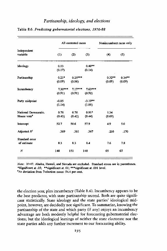
Partisanship, ideology, and elections
Table 8.6. Predicting gubernatorial elections, 1976-88
Independentvariable
Ideology
Partisanship
Incumbency
Party midpoint
National Democratic.House votea
Intercept
Adjusted R2
Standard errorof estimate
N
All contested races
(1)
0.13(0.17)
0.21*(0.09)
7.30***(0.91)
-0.85(114)
0.78(0.43)
52.7
.389
8.3
148
(2)
0.25***(0.06)
7.17***(0.91)
0.78(0.42)
50.6
.381
8.3
151
(3)
0.40**(0.14)
7.63***(0.92)
-3.19**(1.08)
0.91*(0.44)
57.9
.367
8.4
148
Nonincumbent races only
(4)
0.32**(0.09)
1.34(0.69)
4.9
.205
7.6
65
(5)
0.34**(0.09)
5.0
.170
7.8
65
Note: N=47. Alaska, Hawaii, and Nevada are excluded. Standard errors are in parentheses.* Significant at .05; **significant at .01; ***significant at .001 level.aAs deviation from 7-election mean: 54.4 per cent.
the election year, plus incumbency (Table 8.6). Incumbency appears to bethe best predictor, with state partisanship second. Both are quite signifi-cant statistically. State ideology and the state parties' ideological mid-point, however, are decidedly not significant. To summarize, knowing thepartisanship of the state and which party (if any) enjoys an incumbencyadvantage are both modestly helpful for forecasting gubernatorial elec-tions; but the ideological leanings of neither the state electorate nor thestate parties adds any further increment to our forecasting ability.

Statehouse democracy
Table 8.7. Predicting U.S. Senate elections, 1976-88
Independentvariable
Ideology
Partisanship
Incumbency
Party midpoint
National DemocraticHouse vote8
Intercept
Adjusted R2
Standard errorof estimate
N
All contested races
(1)
0.05(0.16)
0.40***(0.08)
7.72***(0.72)
0.88(1.24)
1.20***(0.34)
48.6
.471
9.0
208
(2)
0.34***(0.06)
7.97***(0.72)
1.30***(0.34)
48.5
.470
9.0
213
(3)
0.54***(0.14)
8.20***(0.75)
-3.05**(1.03)
1.10**(0.35)
58.3
.430
9.4
213
Nonincumbent races only
(4)
0.38**(0.14)
1.00(0.75)
47.9
.114
10.1
51
(5)
0.36*(0.14)
48.1
.100
10.2
51
Note: Standard errors are in parentheses.•Significant at .05; **significant at .01; ***significant at .001.aAs deviation from 7-election mean: 54.4 per cent.
However, it does not follow that the electorate's and the parties' ide-ologies are electorally insignificant in state contests. We can manipulatethe equation to get both to emerge as significant contributors to the vote -by omitting state partisanship from the equation. See Table 8.6, Column3. Ideology does matter, at least indirectly. Note also that the .13 coeffi-cient for ideology in the equation from Column 1 is about two-thirds thesize of the partisanship coefficient. The estimate of the ideology coeffi-cient is wobbly, however, as reflected by its larger standard error.
196

Partisanship, ideology, and elections
Next, we turn to the estimation of short-term forces. For each equationin Table 8.6, the standard error of estimate is a measure of the standarddeviation of the election forecast based on the equation at hand. Thus,except for the influence of incumbency, the standard error of estimate is arough index of the short-term forces of the campaign. In the gubernatorialequations, the standard error is in the range of 8 percentage points. This isslightly larger than the 6.5 standard deviation for the national presidentialvote. What can be concluded from this comparison? Suppose one knowsthe incumbency status of a gubernatorial election, plus the state's partisanmakeup and the partisan trend for the particular election year. Althoughthat is a lot of information, it still is not a good predictor of the guber-natorial election. In fact, the forecasting error is greater than predicting apresidential election outcome based on no information other than thelong-term mean of presidential vote outcomes.
Counting incumbency effects as part of the short-term forces makesthese forces loom even larger. Suppose we sum each gubernatorial con-test's residual vote and incumbency effect (each from the equation in Col-umn 2). The resultant standard deviation is 9.7, for a considerableincrease in the estimate of short-term forces.
We might expect the weakest short-term forces in nonincumbent races,where incumbency is no factor and candidates are presumably less wellknown. We should pay special attention, therefore, to the two equationsfor nonincumbent gubernatorial races, of which there were 65,1976-88.For nonincumbent races, the best fit is the equation predicting the votefrom partisanship plus House vote control for the electoral trend, shownin Column 4. Note that the standard error for even this equation, y.6,slightly exceeds the observed standard deviation of national presidentialvote outcomes. Comparing the two as estimates of short-term forces, wearrive at a provocative conclusion: Open-seat elections for governor aremore unpredictable than national presidential contests.
To summarize, state-level party identification does influence the out-comes of elections for governor. But, although state partisanship directlymatters while state ideology does not, this effect of partisanship is smallrelative to the short-term forces of the gubernatorial campaign. Evencounting only "open" races without an incumbent, and controlling for thenational trend, a state's vote divisions for governor will generally varymore than will the national division of the two-party vote for president.
Predicting Senate electionsNext we consider the results for Senate elections, 1976-88, shown inTable 8.7. For Senate elections, we can account for almost half of thevariance in the vote. This "improvement" is largely due to the fact thatsenatorial elections produce more variance to explain.
197

Statehouse democracy
In other respects, the pattern for Senate elections closely parallels thatfor gubernatorial elections. State ideology and party elite ideology do notseem to matter, except when state partisanship is omitted from the equa-tion. Party identification clearly matters, to a slightly greater degree thanfor governor. Incumbency matters too, at about the same magnitude as forgovernor. Incumbency is worth about 8 percentage points to the advan-taged party.
We estimate the short-term forces for senator to be greater than thosefor governor. As estimated by the standard error of estimate, the short-term forces for senator are about 9.0. As estimated by the standard devia-tion of the incumbency effect plus the residual vote (from the equation inColumn 2), the short term forces rise to to 11.3. Finally, even Senate elec-tions for open seats appear quite immune from easy prediction, showing a10.1 standard error of estimate.
To summarize, for Senate elections (as for gubernatorial elections), stateparty identification summarizes all that is relevant about the electorate'sand the parties' relative ideological leanings. For Senate elections (as forgubernatorial elections), omitted variables account for much of the vari-ance in outcomes. Clearly, "short-term forces" - the stimuli of the specificcontest - matter.8
8. The importance of short-term forces in state elections can be appreciated even with-out a direct measure of state partisanship. Consider the state-level correlations be-tween the votes for senator and for governor in the same election year. To the extentthat elections are decided by state partisanship (or any state-level variables), the votedivisions for the two offices should be correlated. To the extent that elections aredecided by short-term forces unique to the specific campaigns, the vote divisions forthe two offices should be uncorrelated. In actuality, the two sets of votes are remark-ably uncorrelated. Over the five midterm election years, 1966-86, the average cor-relation between the gubernatorial and senatorial vote divisions is a feeble .14.Details follow:
19661970
1974197819821986
•24-.12
•15.48.05.O6
(N=23)(N=22)(N=22)(N=26)(N=23)(N=23)
A similar test is to examine the correlation between the state votes for U.S. Senate insuccessive elections. (Short-term forces in the two elections should be independentbecause they represent the votes for two different Senate seats.) These correlations areas follows:
1966-81968-701970-21972-41974-61976-8
.22(N=14)
. i 3 ( N = i 8 )
. 5 9 ( N = i 8 )
.26 (N= 16)
.06 (N= 16)- .n(N=i 4 )
1978-801980-21982-41984-61986-8
.o 9 (N=i 4 )-.09 (N= 15)
.09 (N= 17)
. i 7 (N=i6)
.25(N=15)
198

Partisanship, ideology, and elections
Ideology and partisanship in individual state electionsSo far we have examined state contests solely at the aggregate level. As wedid for presidential contests, we can also examine individual-level votingdata from exit polls of state-level gubernatorial and senatorial contests.Between 1982 and 1988, CBS/NYT conducted 41 exit polls of guber-natorial elections and 69 exit polls of senatorial elections that ascertainedrespondents' partisan and ideological identifications. For each exit pollsurvey, we conducted a probit equation predicting the vote from partisanand ideological identification. The results of these 110 equations areshown in Tables 8.8 (for governor) and 8.9 (for senator). For a referencepoint, these equations can be compared to the comparable presidential1984 and 1988 equations, presented in Table 8.3.
The first thing to note from these tables is the dominant role of partyidentification at the individual level. In all 110 equations, the probit coeffi-cient for party identification exceeds the coefficient for ideology. Themean party identification coefficient is 0.84 (0.80 for governor, 0.87 forsenator), somewhat below the 1.03 coefficient for the presidential vote inthe 1988 exit poll. Variation in the partisanship coefficient tracks thedegree to which the specific contest taps traditional partisan issues. Thehighest coefficient is a 1.26 in the Bond-Woods 1988 Missouri Senatecontest, in which Harriet Woods conducted a strongly populist campaign.The weakest is for the Weicker-Lieberman 1988 Connecticut Senate con-test in which the Democrat was arguably to the right of his Republicanopponent.
Although overshadowed by partisanship, ideological identification alsoinfluences votes for senator and governor. Just because state ideology doesnot forecast aggregate state election outcomes (once party identification iscontrolled), we should not be surprised to find that individual voters'ideologies predict their votes in state elections. In 108 of the 110 equa-tions, the ideology coefficient is positive. The average coefficient is0.37, somewhat less than the 0.52 and 0.67 found for the 1984 and 1988presidential races. One could make the plausible argument that sincegubernatorial campaigns deal with state issues, they should be less ideo-logical than senatorial campaigns, which necessarily involve national is-sues. However, such a pattern is not found for the ideology coefficients.On average, the ideology coefficient is 0.35 for governor, and 0.38 forsenator.
The ideology coefficient varies across contests, with a standard devia-tion of 0.16, which is identical to the standard deviation of the partisan-ship coefficient. The size of the ideology coefficient reflects the degree ofideological division in the particular campaign. The strongest ideologyco fficient for a gubernatorial contest is 0.62, found for two campaigns
199

Table 8.8. Probit equations of CBS/NYT governor exit polls, 1982-88
Probit Coefficients
State
AL
AZ
AR
CACA
CO
CN
FL
GA
ILIL
IN
IA
Year
1982
1986
1982
19821986
1986
1982
1986
1986
19821986
1988
1982
RepublicanCandidate
Fulmar
Mecham
Whitea
DeukmejianDeukmejian8
Strickland
Rome
Martinez
Davis
Thompson11
Thompson8
Mutz
Branstad
DemocraticCandidate
Wallace
Warner
Clinton
BradleyBradley
Romer
O'Neill
Pajcic
Harris8
StevensonStevenson
Bayh
Conlin
DemocraticVote
.60
.47
.55
.49
.38
.59
.54
.45
.71
.50-
.43
.53
.47
PartyIdentification
0.99
0.83
0.67
0.760.87
0.82
0.72
0.97
0.50
0.881.05
0.84
0.76
IdeologicalIdentification
0.25
0.62
0.50
0.440.54
0.32
0.23
0.42
0.27
0.220.18
0.47
0.45
Constant
-0.01b
0.06b
-0.07b
-0.07-0.29
0.41
0.03
-0.07b
0.75
-0.13-0.13
0.41
-0.05b
N
1,695
750
111
2,9332,445
1,198
1,949
1,411
599
1,4851,018
1,073
1,074

ME
MA
MI
MN
MO
NE
NVNV
NH
NM
NYNY
NCNC
OH
OR
PA
1982
1982
1982
1982
1988
1982
19821986
1984
1982
19821986
19841988
1982
1986
1986
Craggin
Sears
Headlee
Whitney
Ashcrofta
Thonea
Lista
Caffarata
Sununua
Irick
LehrmanO'Rourke
MartinMartin8
Brown
Paulus
Scranton
Brennana
Dukakis
Blanchard
Perpich
Heames
Kerrey
BryanBryana
Spirou
Anaya
CuomoCuomoa
EdmistonJordon
Celeste
Goldschmidt
Casey
.62
.62
.53
.59
.35
.51
.56
.74
.33
.53
.52
.67
.46
.44
.60
.52
.51
0.73
0.88
1.00
0.99
0.79
0.73
0.650.59
0.84
0.68
0.700.57
0.770.92
1.00
0.56
0.80
0.28
0.58
0.35
0.16
0.34
0.42
0.260.19
0.18
0.44
0.440.36
0.540.39
0.41
0.34
0.02b
0.31
0.21
0.03b
0.20
-0.46
0.20
0.130.86
-0.36
0.05b
-0.01b
0.57
-0.21-0.21
0.36
0.13
0.04b
1,475
2,750
813
1,129
867
1,166
1,077977
560
1,124
2,3061,363
1,6321,325
922
763
1,346

Table 8.8. (continued)
State
RI
SD
TN
TXTX
VTVTVT
WA
WV
WY
Year
1982
1986
1982
19821986
198219841988
1988
1984
1982
RepublicanCandidate
Marzullo
Mickelson
Alexander*
Clementsa
Clements
Snelling8
EastonBemhardt
Williams
Moore
Morton
DemocraticCandidate
Garrahya
Herseth
Tyree
WhiteWhite8
KunenKunenKunena
Gardner8
See
Herschler8
DemocraticVote
.76
.48
.40
.54
.47
.44
.51
.55
.62
.47
.63
Probit Coefficients
PartyIdentification
0.76
0.80
1.07
1.020.94
0.820.710.62
0.71
0.80
0.81
IdeologicalIdentification
0.19
0.08b
0.41
0.520.36
0.380.510.47
0.62
0.08b
0.18
Constant
0.72
-0.02b
-0.41
-0.07b
-0.14
0.03b
0.120.31
0.48
-0.35
0.62
N
1,147
917
826
1,9801,435
1,056826680
780
989
872
Note: aIncumbent. bnot significant at .05.

Partisanship, ideology, and elections
with unusually strong infusions of ideology. One is Arizona's 1986 con-test, won by archconservative and ideologically contentious EdwardMechem. The other is Washington's 1988 contest, in which the Republi-can primary produced a follower of Evangelist Pat Robertson to opposeDemocratic Governor Booth Gardner. The strongest ideological coeffi-cient for a senatorial contest is found for the ideologically polarized 1984Helms-Hunt North Carolina contest. The 0.73 ideology coefficient forthe Helms-Hunt race is the only one that exceeds the ideology coefficientof the 1988 presidential contest (0.67 - see Table 8.3.)
At the other extreme, particularly weak ideological coefficients arefound for those campaigns either devoid of ideological content or wheretraditional partisan-ideological battle lines were confused. For governor,the weakest coefficient (.02) is for Pennsylvania's 1986 Casey-Scrantoncontest, in which Democrat Casey posed as the more culturally conserva-tive candidate. For senator, we find the two negative coefficients, in theaforementioned Weicker-Lieberman race and for Packwood of Oregon's1986 reelection. Both contests featured a moderate-to-liberal Republicanincumbent. Low positive coefficients are found for other Senate contestsinvolving moderate incumbents, for instance, Chafee, Hatfield, Heinz,and Spector among Republicans and Dixon, Stennis, and Zorinski amongDemocrats.
That ideologically polarized candidates generate a more ideologicalelectorate can be demonstrated statistically, following Wright and Berk-man (1986). For one set of contests, we have a numerical measure of theideological division of the candidates, which can be related to the ideologycoefficient. For all 1982 Senate candidates, CBS/NYT ascertained opin-ions on a set of 10 ideologically relevant issues. We combined the re-sponses to create a 10-item scale. Then we computed an ideologicalpolarization score as the difference between the ideological position of thestates' Democratic and Republican candidates. For the 23 Senate contestsin 1982 for which we have exit poll data, we computed the correlationbetween this measure of ideological polarization and the ideology coeffi-cient from the exit poll equation. This correlation is a healthy .64. Ideol-ogy matters more in elections that offer a choice to state voters.
Because Democrats outnumber Republicans and conservatives out-number liberals, a plausible line of reasoning is that highly partisan con-tests work to the Democrats' advantage while highly ideological contestsfavor the Republicans. Thus, one might expect that Democratic candi-dates gain from a strong partisanship coefficient and Republicans gainfrom a strong ideology coefficient. But neither tendency is evident fromthe data. The Democratic vote correlates at -.18 (wrong sign) with thepartisan coefficient and -.01 with the ideology coefficient. Clearly, elec-tions are not won or lost based on candidates' ability to manufacture
203

Table 8.9. Probit equations of CBS/NYT Senate exit polls, 1982-88
Probit Coefficients
State
AL
AZ
CACACA
CO
CNCN
FL
GA
ILIL
IN
IA
LA
Year
1984
1986
198219861988
1986
19821988
1986
1986
19841986
1988
1984
1988
RepublicanCandidate
Smith
McCain
WilsonZchauWilson8
Kramer
Weicker8
Weicker8
Hawkins
Mattingly8
Percy8
Koehler
Lugar8
Jepson8
Moore
DemocraticCandidate
Heflin8
Kimball
BrownCranston8
McCarthy
Wirth
MoffettLieberman
Graham
Fowler
SimonDixon8
Wicks
Harkin
Breaux
DemocraticVote
.63
.40
.47
.51
.47
.51
.48
.50
.55
.51
.51
.66
.32
.56
.53
PartyIdentification
0.69
0.95
0.861.051.01
0.95
0.640.35
0.69
1.07
0.940.92
1.01
1.06
0.89
IdeologicalIdentification
0.29
0.47
0.520.500.56
0.58
0.07b
-0.06b
0.34
0.47
0.390.18
0.49
0.30
0.39
Constant
0.33
-0.11
-0.230.07
-0.05b
0.14
-0.15-0.03b
0.19
-0.09b
0.06b
0.44
-0.68
0.31
-0.09b
N
1,330
1,083
2,8822,4372,031
1,196
1,9151,125
1,427
624
1,7141,034
840
1,623
1,132

ME
MD
MAMAMA
MIMIMI
MNMNMN
MSMSMS
MOMO
MT
NE
NVNVNV
NH
1982
1988
198219841988
198219841988
198219841988
198219841988
19821986
1982
1982
198219861988
1984
Emery
Keyes
ShamieShamieMalone
RuppeLousmaDunn
Durenberger8
Boschwitz8
Durenberger51
BarbourCochran8
Lott
Danforth8
Bond
Williams
Keck
HechtSantiniHecht8
Humphrey8
Mitchell
Sarbanesa
Kennedy8
KerryKennedy8
Riegle8
Levin8
Riegle8
DaytonGroweHumphrey
Stennis*WinterDowdy
WoodsWoods
Melcher8
Zorinsky8
Cannon8
ReidBryan
D1 Amours
.61
.62
.61
.55
.66
.59
.52
.61
.47
.42
.42
.64
.39
.46
.49
.47
.57
.70
.49
.53
.52
.41
0.87
0.82
0.860.900.74
0.871.020.83
0.941.170.98
0.540.910.83
0.921.26
0.84
0.71
0.791.090.70
0.83
0.30
0.49
0.620.560.63
0.15b
0.390.42
0.420.390.33
0.210.470.37
0.370.46
0.40
0.10b
0.380.310.46
0.28
0.24
0.12-0.110.32
0.150.210.58
-0.27-0.39-0.26
0.28-0.43-0.20
-0.15-0.07b
0.25
0.75
-0.07b
0.150.14
1,516
1,019
2,8221,3561,061
8281,0531,280
1,1751,2761,001
9561,139
976
2,0341,189
1,327
1,120
1,117973767
0.46 -0.11 602

Table 8.9. (continued)
State
22
2
NMNM
NYNYNY
NCNC
ND
OHOH
OROR
PAPA
Year
198219841988
19881988
198219861988
19841986
1986
19821988
19841986
19861988
RepublicanCandidate
FenwickMocharyDawkins
Schmidt8
Valentine
SullivanD'Amato8
McMillan
Helms8
Broyhill
Andrews8
PfeiferVoinovich
Hatfield8
Packwood8
Specter8
Heinz8
DemocraticCandidate
LautenbergBradley8
Lautenberg8
BingamanBingaman8
Moynihan8
GreenMoynihan8
HuntSanford
Conrad
Metzenbaum8
Metzenbaum8
HendriksenBauman
EdgarVignola
DemocraticVote
.51
.65
.54
.54
.63
.66
.42
.68
.48
.52
.50
.58
.57
.33
.36
.43
.33
Probit Coefficients
Party IdeologicalIdentification Identification
0.870.920.94
0.810.71
0.650.720.67
0.741.09
1.10
0.900.88
0.620.61
0.900.76
0.110.380.32
0.390.35
0.400.470.66
0.730.61
0.32
0.540.43
0.25-0.02b
0.270.25
Constant
0.01b
0.560.14
-0.020.45
0.70-0.360.78
-0.03b
0.00b
0.13
0.280.26
-0.53-0.39
-0.27-0.66
N
1,9961,3801,193
1,9961,132
1,1211,3431,502
1,7451,148
957
9331,353
1,331753
1,3671,356

RI
SD
TN
TXTXTX
UT
VTVT
VA
WA
WVWV
WI
WY
1982
1986
1982
198219841988
1982
19821988
1982
1988
19821984
1988
1982
Chafee8
Abnora
Beard
CollinsGrammBoulter
Hatca
Stafford8
Jeffords
Trible
Gorton
BenedictReese
Engeleiter
Wallop8
Michaelson
Daschle
Sasser8
Bentson8
DoggettBentsen8
Wilson
GuestGray
Davis
Lowry
Byrda
Rockefeller
Kohl
McDaniel
.49
.52
.62
.59
.41
.60
.42
.48
.31
.49
.48
.69
.52
.52
.43
0.90
0.98
1.01
0.821.070.93
1.06
0.820.39
1.10
0.93
0.980.79
0.73
0.83
0.15
0.44
0.28
0.490.640.47
0.51
0.170.18
0.36
0.62
0.360.18
0.31
0.29
-0.18
0.23
0.19
0.21-0.230.46
0.10
0.04b
-0.56
-0.07b
-0.03b
0.45-0.14
0.06b
-0.05b
1,262
934
1,262
1,9731,8001,720
1,534
1,056651
939
966
632971
1,239
873
Note: aIncumbent. bnot significant at .05.

Statehouse democracy
partisan or ideological heat. Instead, as we will see, it is the relative ideo-logical placement of the candidates that matters.
A crucial statistic in Tables 8.8 and 8.9 is the intercept. Each interceptreflects the behavior of voters at "zero" on both partisanship andideology - in other words, given our scoring procedure, the behavior of"moderate Independents." Where the coefficient is positive, most of these"neutral" voters voted Democratic. Negative coefficients indicate thatmost moderate Independents voted Republican. The standard deviationof the 110 intercepts is 0.32, with a range from -0.68 to 0.86. For com-parison, the intercept of the 1988 presidential race is only -0.06. Moretellingly, the intercept for Reagan's 1984 landslide was only -0.30. Inter-cepts with absolute values greater than 0.30 are found for 35 of the 110state exit poll equations. By this test, the short-term forces of guber-natorial and senatorial contests exceed those of the 1984 Reagan landslideabout one-third of the time.
For all practical purposes, the intercept predicts the election outcome. Itcorrelates at .91 with the Democratic vote. In the overwhelming propor-tion of the contests (97 of 110), the direction of the intercept predicts theelection winner. Thus, the collective decisions of moderate Independentsis almost always electorally decisive. An interesting implication is, onceagain, that state ratio of Democrats to Republicans (or of conservatives toliberals) is of lesser electoral significance. It is short-term forces generatedby the candidates that matter most.
Candidate appeal is determined by many factors. Incumbents usuallyobtain positive coefficients (56 out of 67), but incumbency may be aneffect as well as a cause of candidate popularity. Other factors such ascandidates' charisma, cash, and possible taint of scandal also contributeto short-term forces (Abramowitz, 1988). Among these other factors wealso find the ideological positions of the candidates. Careful perusal ofTables 8.8 and 8.9 suggests that moderate candidates tend to obtain favor-able intercepts and win elections.
Following our usual logic, our expectation is that the more liberal thetwo candidates are, the better the Republican candidate should do. Wecan test this notion empirically using the liberal-conservative scores of1982 Senate candidates. For the 23 races for which we have relevant data,the correlation between the candidate midpoint on the 10-point ideologi-cal scale and the intercept of the state's individual voter equation is ahealthy .51. This correlation holds up for the subsample of Republicanincumbents (r = .56; N - 8) but dissipates for Democrats (r = .17; N = 11).Within each party, sitting senators tend to be more moderate than sen-atorial challengers. A suspicion is that their moderation allows Senators tostay elected.
2 0 8

Partisanship, ideology, and elections
CONCLUSIONS
The partisan division of a state is electorally important. Recall, for in-stance, that state partisanship is a strong predictor of the relative strengthof the two parties in the state legislature. Over time, a strongly Democra-tic or strongly Republican state will find its state legislature almost alwayscontrolled by the dominant party. The reason is that short-term forces inindividual legislative races cancel out, while state-level issues only mod-estly affect legislative election outcomes. All this leaves state party identi-fication as the natural predictor of legislative control. If state partisanshipdetermines legislative control, it might seem to follow that state partisan-ship works to retard the process of representation in the states. We offer aquite different interpretation. The relative strengths of the Democraticand Republican parties within a state electorate reflect their relative suc-cess at representing state opinion.
This chapter has examined state elections by focusing on state-levelvoting for president, governor, and senator. Our investigation has high-lighted both the importance and the limitations of state partisanship as apredictor of state election outcomes. State partisanship takes on specialimportance because it reflects the relative ideological proximity of thestate electorate to the two major political parties. In presidential elec-tions, however, state electorates appear to discount that portion of theirpartisanship that is traceable to the ideological locations of their stateparties.
Although important, state partisanship leaves vast amounts of theunexplained variance in state outcomes, particularly in elections belowthe presidential level. State elections for senator and governor are largelythe result of short-term forces independent of state partisanship. Set-ting knowledge of the candidates aside, state elections are more diffi-cult to forecast from partisanship alone than national presidential elec-tions are from knowing only the post-World War II partisan trackrecord.
We illustrate this important point with one final set of electoral scat-terplots. Figure 8.5 shows the statistically significant but weak relation-ships between state partisanship and the vote in nonincumbent races forgovernor and the U.S. Senate. The regression lines are borrowed fromColumn 5 of Tables 8.6 and 8.7. Since these are all races without anincumbent candidate, we might expect that candidate-generated short-term forces would be weak, and the election would be relatively safe forthe dominant party where one party holds a clear edge in party identifica-tion. Note, instead, the wide variation around the regression lines. Given
2 0 9

Statehouse democracy
20
-20 0 20 40
State Party Identification (Dem. - Rep.)
80"
60"
40"
20"
Senatorial Contests
o
oo
o
° o cpoo
o o °o
o
o
o
o
^ ^
o
Q> O
o
o
CO °oo
-20 0 20 40
State Party Identification (Dem. - Rep.)
Figure 8.5 Predicting Open Seat Electoral Outcomes for Governor and U.S.Senator from State Party Identification, 1976-88
2 1 0

Partisanship, ideology, and elections
the positive regression lines for party identification, we can certainly con-clude that owning a lead in party identification helps a party in stateelections. But the benefit is marginal. Throughout the U.S. states, voters'party loyalties are sufficiently weak to allow both parties to achieve com-petitive stature in major state elections.
2 1 1

State opinion over time
So far, our discussion has focused solely on political life in the states as it isquantified for the late 1970s and the 1980s. The present chapter expandsthe focus backward in time, in order to place our findings in historicalperspective. For this task, we assemble measures of state ideology andpartisanship from earlier eras. These measures, drawn from Gallup pollsfrom 1936 to 1963, are far noisier than the contemporary measures ofstate ideology and partisanship that have dominated our discussion so far.
Measurement error demands that our indicators of "historical" ideol-ogy and partisanship be analyzed with considerable care. Still, Gallup-based measures of early ideology and partisanship provide helpful lever-age for understanding the historical continuity of state-level public opin-ion and its consequences - from the times of the New Deal to the Reaganpresidency. In the following pages, we will see that earlier state-level ideo-logical sentiment may have been less stable than we found for the morerecent period, 1976-1988. We will also see evidence that even for the1930s to the 1960s, state ideology was an important influence on statepolicy.
HISTORICAL MEASURES OF STATE OPINIONChapter 2 demonstrated that for the 13 years from which our CBS/NYTsurvey data were collected, states moved very little in terms of their rela-tive positions on the scales of net ideological identification and partisanidentification. The stability of the states was particularly evident in thecase of ideology. We might imagine that our measure of the ideologicalpreferences of state electorates captures a cleavage in state-level publicopinion so enduring that it has been present for decades. Still, we mustconsider the possibility that the ideological ordering of the states has notalways been stable. Thus, we expand our time horizon backward morethan 50 years in a search of an evolutionary change in the way statepublics orient themselves ideologically.
212

State opinion over time
Gallup polls: 1937-64
Because it has regularly monitored Americans' political beliefs since themid 1930s, the Gallup poll is the obvious data source to estimate thepartisanship and ideology of state electorates prior to 1976. With the aidof the Roper Center for Public Opinion Research, we were able to identify19 national Gallup polls conducted between 1937 and 1964 that con-tained questions about the ideological preferences of respondents. Theirregularity with which Gallup (and other pollsters) probed ideologicalpreferences during this earlier era is far different from current practice.Indeed, for the eventful period from 1964 to 1969, Gallup evidently didnot ask an ideological question once. This drought is the reason why oursporadic series of historical ideological observations stops in 1964.
Almost half of the long-term "sample" for our historical readings ofideology come from seven surveys from the prewar 1937-39 period. Weaggregate these seven surveys, with 19,119 usable ideological responses, toconstruct a measure of pre-World War II state opinion. We also aggregatethe post-World War II portion of our historical sample, composed of29,465 usable ideological responses from 12 Gallup surveys between 1947and 1964. Thus, we have measures of ideology for three periods:
pre-World War II (1937-9),post-World War II (1947-64), andcontemporary (1976-88).
The ideological questions that Gallup asked were not today's standardquestion regarding ideological identification as a liberal, moderate, orconservative. In some variant, 7 of the surveys asked respondents whethertheir political views were liberal or conservative, without encouraging amoderate or middle-of-the-road response. The remaining 12 surveys,again with variation in question wording, offered respondents a hypo-thetical choice of two ideological parties in place of the standardDemocrats and Republicans. Respondents were asked whether theywould join or prefer the party for liberals or the party for conservatives.Survey dates and exact question wordings are presented in the appendixto this chapter. For the prewar surveys, party identification was not reg-ularly asked. Consequently, we offer no measure of state partisanshipfrom the 1930s here. After World War II, however, Gallup monitoredparty identification regularly. Thus, from the 12 surveys from which wedrew estimates of postwar state ideology, we also obtained estimates ofpostwar state partisanship.
For our historical samples we measured ideological and partisan identi-fication in our customary way. Counting liberal responses as +100, in-between or neutral responses as o, and conservative responses as -100, wecomputed state means, which can also be interpreted as percentage point
213

Statehouse democracy
differences - percent liberals minus percent conservatives. Similarly, wecomputed state party identification in the usual way as the state mean ofDemocratic (+100), Independent (o), and Republican (-100) responses.
Methodological problemsComparing state means from contemporary CBS/NYT polls with statemeans from earlier Gallup polls presents certain hazards. We must con-sider differences due to ordinary house effects, differences in questionwording, and differences in sampling procedure. In addition, we must besensitive to the much lower Ns from the pooled Gallup series. The mostserious pitfall, however, from the standpoint of estimating state means, isthe greater geographic clustering of respondents for in-person surveys ofthe earlier era.House effects. Studying historical trends based on polling data fromdifferent survey research organizations presents a hazard of uncertainmagnitude. Even when different organizations attempt to measure thesame public sentiment at exactly the same point in time, their estimatesoften diverge. These differences are usually attributed to "house effects,"or the marginal variation in response achieved by different survey teams.House effects include not only variation in exact question wording and insampling procedure (discussed separately in upcoming sections), but alsosuch details as differing approaches to handling nonresponses, contextual(question-order) effects, interviewer training and supervision, and codingdecisions. Historical trend analysis that requires use of data collected bymore than one survey firm runs the risk of mistaking house effects for truechange (Smith, 1978, 1982, 1987; Converse and Schuman, 1984; Turner,1984).Question wording. Survey researchers now recognize that even seeminglyminor variations in how questions are worded can have surprisingly largeeffects on survey answers. Thus, differences in question wording over thetime span of our historical analysis deserve special consideration. To con-sider the mildest example first, Gallup and CBS/NYT preface their "partyidentification" question differently. Gallup asks respondents whether "inpolitics as of today" they consider themselves to be Democrats, Indepen-dents, or Republicans. CBS/NYT asks respondents whether "generallyspeaking" they regard themselves as Democrats, Independents, or Re-publicans. Fortunately, it turns out that the Gallup and the CBS/NYTvariants produce virtually identical distributions of partisanship over time(MacKuen, Erikson, and Stimson, 1992). This result only reinforces ourconfidence that the two variants of the party identification questionshould order the states similarly on the partisan continuum.
But what about the crucial variable of ideological preference? In recentyears, Gallup and CBS/NYT have asked similar questions concerning re-
214

State opinion over time
spondent identification as liberal, moderate, or conservative. The contem-porary menu of "liberal," "moderate," or "conservative" was not thechoice offered by Gallup in our historical samples. As mentioned, somewere asked whether they considered themselves a liberal or conservative,with no clear middle alternative. Others were asked whether they wouldprefer a liberal or a conservative party.
Conceivably, the national division of ideological sentiment depends insome important way on the exact question asked. In terms of state meanscores, Gallup's earlier questions should generate greater variance becauseof their discouragement of the middle position. For our purposes, how-ever, the most crucial question concerns not the metric but whether states'relative positions on the ideological continuum vary with exact questionwording. That sort of contamination strikes us as relatively improbable.Although differences in wording may affect the percentage, say, of bothNew Yorkers and Indianans who call themselves liberal or conservative,the relative rankings should hold constant across minor question formatdifferences. New York ought to score considerably more liberal than Indi-ana as long as the questions tap the same underlying dimension of liberal-conservative ideology. Consequently we see little risk in comparing statemeans from different surveys that measure ideological sentiment withdifferent questions.Sampling, Changes over time in standard survey procedure present anadditional reason for caution. Changes over time in the pattern of surveyresponses may actually be artifacts of sampling methodology. Like otherpolls of the era, early Gallup polls relied on "quota" sampling techniques(Gallup, 1948, 1972; Frankel and Frankel, 1987). In the aftermath of themiscall of the 1948 election, many firms removed the power to choosesubjects from their interviewers and adopted strategies designed to ensurerandom selection of interviewees within tightly drawn population clus-ters. The 1970s saw a second revolution in sampling strategies as inter-viewers were pulled off the street and assigned to call randomly selectedtelephone numbers. Random digit dialing, while incorporating the cluster-ing approach, permitted contact with a greater number of geographicallydispersed clusters (Waksberg, 1978). Each of these shifts in samplingstrategy has the potential to distort inferences about true change overtime.
One special source of sampling change over time is the shift of theuniverse that the sample is supposed to represent. Early Gallup polls,designed to reflect the composition of the electorate, underrepresentedwomen and minorities relative to their proportion of the population(Glenn, 1975; Glenn and Frisbie, 1977). Yet these early polls reasonablyreflect the composition of the voting electorate at the time. We must becareful to understand just what we are measuring and what comparisons
215

Statehouse democracy
may be made with these data. Our early state-level estimates will reflectthe states' voting electorates of the time. Our later CBS/NYT state sam-ples more closely reflect the general population.Sample sizes. A serious concern regarding the state- level prewar and post-war Gallup estimates is the "small" sample sizes involved. Aggregatednational samples of 19,169 and 29,465 would not normally be calledsmall, except in comparison to our mammoth aggregation of over150,000 respondents for our contemporary measures of state ideologyand partisanship. Quite obviously, the statistical reliability of the histor-ical estimates is much lower than for the contemporary measures.Clustering. More than sample size affects the statistical reliabilities of ourGallup-based state estimates. The reliabilities of the historical estimatesare further compromised because of the practice by Gallup (and otherpollsters) of clustering respondents geographically for in-person inter-views. Survey organizations typically cluster respondents for a nationalsurvey in as few as 80 primary sampling units or PSUs (counties orSMSAs), and even by specific neighborhoods within PSUs. For reasons ofcost, survey researchers will often maintain the identical clusters for yearson end. As a result, even when aggregated over years, state subsamples areclustered by geography.
The potential consequences of this sampling procedure include severedistortion of state-level estimates. For any state, it is conceivable that allrespondents for a decade or more may reside in a small number of ar-bitrarily selected counties - and perhaps even from a small number ofneighborhoods within those counties. Thus, a procedure that is sensiblefor interviewing a national sample of respondents in their homes offers theuncertainty of some unknown bias when used for what it is not designedfor - estimating the breakdown of opinion by state. Put simply, Gallup'sstate-level mean estimates are even less reliable than the number of re-spondents per state would indicate.
This problem of severe clustering separates the Gallup-based measuresof historical opinion from our contemporary CBS/NYT measures. Asdiscussed in Chapter 2, sample clustering is a lesser problem for the con-temporary telephone surveys conducted by CBS/NYT. With samplingfrom repeated draws of a large number of telephone exchanges, over-timeaggregations of CBS/NYT telephone surveys offer reasonable approxima-tions of representative samples within states.
From this discussion, it should be clear that the earlier Gallup-basedmeasures of state opinion are considerably inferior to the CBS/NYT-based measures that we use for our contemporary analysis. As we will see,however, this caveat certainly does not mean that the historical measuresare of little value. In the following pages, we use the historical opinion
2 1 6

State opinion over time
measures to gather clues about the stability of state opinion over time andabout the stability of the representational process.
LONG-TERM STABILITY OF STATE IDEOLOGY AND
PARTISANSHIP
Correlations representing the long-run relative stability of ideology andpartisanship are presented in Table 9.1. These correlations are presentedfor three sets of states. The first set is all 47 (Nevada excluded) continentalstates. The second set includes only the 30 (Nevada excluded) northern(nonsouthern, nonborder) states only. The third includes only the 12 larg-est northern states, which each contain a combined prewar and postwarsample of a thousand or more respondents.1 The culling of first southernand border states and then small states serves two obvious purposes.Deleting southern states (and border states as well) controls for the inter-esting sectional evolution of the South toward both conservatism andcompetitive political parties. Deleting small states helps to reduce the sam-pling error for our historical measures of state ideology and partisanship.
The stability of state partisanship, 1947-88
Consider first the relatively simple matter of following state partisanshipover time. We have only two measures of state partisanship - postwar(1947-64) and contemporary (1976-88). As the correlations indicate,state-level partisanship is fairly stable over the long haul. This conclusionremains when we control for southern sectionalism and for state samplesize. The basic stability of state partisanship can be seen by comparing thepostwar map of state partisanship with the contemporary version (Figure
Relative stability does not imply absolute stability. Figure 9.2 displaysthe scatterplot of the two temporal readings of state partisanship. Thisfigure reveals a certain compression of the distribution of state partisan-ship, mainly from the declining Democratic strength of southern states.Between the postwar and contemporary periods, the range of state meanson party identification compressed to the point that the standard devia-tion of the distribution declined by almost one-half from its former magni-
1. The "large" northern states are California, Illinois, Indiana, Iowa, Michigan, Min-nesota, Ohio, New Jersey, New York, Pennsylvania, and Wisconsin. By the 1970sand 1980s, Iowa would have dropped off this list of largest northern states. Nevadais omitted from the correlation base for comparability with our contemporary analy-sis.
2 1 7

Table 9.1. Over-time correlations of state partisanship and ideology
Ideology Partisanship
Variable Prewar Postwar Contemporary Postwar Contemporary(1937-39) (1947-64) (1976-88) (1947-64) (1976-88)
47 states
Ideology
PrewarPostwarContemporary
Partisanship
PostwarContemporary
MeanS.D.
30 northern states
Ideology
PrewarPostwarContemporary
Partisanship
PostwarContemporary
MeanS.D.
1.00.11.03
.43
.34
-1.711.3
1.00.39.35
.18
.05
-4.711.2
12 large northern states
Ideology
PrewarPostwarContemporary
Partisanship
PostwarContemporary
MeanS.D.
1.00.71.46
.16
.34
-1.76.0
1.00.56
.11
.16
-3.911.7
1.00.57
.61
.51
-4.011.6
1.00.60
.37
.50
-5.38.6
1.00
-.19.08
-14.67.3
1.00
.44
.73
-12.67.4
1.00
.37
.70
-8.94.7
1.00.77
15.121.5
1.00.63
4.015.6
1.00.73
8.09.9
1.00
7.011.4
1.00
1.46.5
1.00
5.45.5

State opinion over time
Postwar
Contemporary
Figure 9.1 Maps of State Partisanship Over Time
2 1 9

Statehouse democracy
50 75
Postwar (1947-64) Party Identification
Figure 9.2 Plot of State Partisanship Over Time. Note: HigherScores Indicate Greater Democratic identification.
tude. See Table 9.1. In part this compression of the variation in statepartisanship scores may be a trick of measurement error, which exagger-ates the observed variance of a variable. Based on sampling consider-ations, we know that the postwar measure of state partisanship should besomewhat contaminated from measurement error. Meanwhile, fromChapter 2 we also know that the contemporary measure of state partisan-ship is relatively free of measurement error. The decline in measurementerror from the postwar to the contemporary readings of state partisanshipcould by itself produce the illusion of a compression of state differences inmass partisanship.
But another likely source of this compression is that the actualdifferences in state party preference did indeed get smaller. In the immedi-ate postwar era, state electoral outcomes favored the dominant party to anextent that would not be imaginable today. Such instances are found al-most entirely in the once one-party (Democratic) South. To an extent notfound today, states were divisible into those with meaningful party com-petition and those without.
220

State opinion over time
The stability of state ideology, 1937-88Chapter 2 showed that within the relatively narrow time range from 1976to 1988, state electorates were quite stable in their ideological positions.Each state held a certain position on the ideological continuum and stayedthere - at least for the 13 years examined. When we look backward over afifty-year span, however, we observe evidence that a remarkable amountof ideological movement occurred.
To appreciate the amount of movement on the ideological scale, oneneed only observe the changes in the ideological map from prewar topostwar to contemporary times, shown in Figure 9.3. Note that the mostliberal states included a strong concentration in the South, while conser-vatism prevailed mainly in rural western and midwestern states. MostNew England states also were on the right, living up to their reputations asbastions of crusty Yankee conservatism. By the postwar reading, theseregional stereotypes had largely faded. By the contemporary reading, anew pattern had emerged: southern and western conservatism versus bi-coastal liberalism.
Figure 9.4 shows this ideological movement via a series of scatterplots.As the figure shows, there is virtually no statistical relationship (r = .11)between the states' prewar and postwar ideological means. Similarly, vir-tually no correlation exists between the prewar configuration of the statesand the ideology of state electorates in the 1980s (r = .03). Even betweenthe postwar measure, 1947-64, and our contemporary measure (1976-88), the correlation is a mere .56.
Even if the true over-time correlations were perfectly stable, we wouldexpect some slippage in the observed correlation due to measurementerror. But appealing on the grounds of bad measurement is an inadequatedefense when observed correlations are near zero. Although the detailsmay be foggy due to inadequacies of measurement, the general contoursare clear: The positions of the states on the liberal-conservative con-tinuum have undergone major shifts, particularly from before to afterWorld War II. To understand these shifts, we should first consider how theideological terms "liberal" and "conservative" were popularly used in the1930s. By the late 1930s, liberalism had already evolved from its classicmeaning of belief in limited government and laissez-faire economics intoits quite different current meaning: a willingness to use government as apositive instrument, particularly to help the disadvantaged. The transfor-mation followed the 1932 presidential election. Both candidates, Hooverand Roosevelt, championed the cause of liberalism and limited govern-ment. Once Roosevelt was elected, the term "liberal" was commandeeredto become a pro-New Deal pro-government action label. Slowly, the op-position rallied to the conservative label (see Rotunda, 1986).
221

Prewar
Postwar
Contemporary
MostConservative
MostUberal
Figure 9.3 Maps of State Liberalism Over Time

20
-40
DE
MENENM
/
OR,
'AWY
KS
AZ
ILMD
sllD
Rl
N Y y /
u / A L
^ A ^
M
LA J X A R
-40 -20 0 20Prewar (1937-9) Mean Ideology
8.
20"
f °12-20
-40
KS y ^fib*
//j NY ™
WL DEAZ
J A l
-40 -20 0 20Postwar (1947-64) Mean Ideology
•40 -20 6 20
Prewar (1937-9) Mean Ideology
Figure 9.4 State Ideology Over Time. Note:Higher scores indicate greater liberalism.

Statehouse democracy
By the late 1930s, the liberal-conservative distinction had become al-most synonymous with the pro- or anti-New Deal distinction. Thus, forour prewar 1937-9 sample, we find Democratic states, including those ofthe South, calling themselves liberal. In fact, the most liberal of the prewarstates were found incongruously (by current standards) in the DemocraticSouth.
At first glance, the liberal characterization of prewar southern (mainlywhite) electorates may appear suspicious. The history of the KKK, re-ligious fundamentalism, and the civil rights battles of the 1950s and 1960scolor historical assessments of the region. But our depiction of the 1930sSouth as liberal is not revisionist history. Consider how V. O. Key's South-ern Politics summarizes the political leanings of the region:Southern liberalism is not to be underestimated. Though southern conservatism isnot entirely a myth . . . fundamentally within southern politics there is a powerfulstrain of agrarian liberalism, now reinforced by the growing unions of the cities. Itis not always perceptible to outsiders - or even to the southerner - because of thecapacity of the one-party system to conceal factional differences. (1949, 670)
One can see this earlier southern liberalism by examining responses tosome of the issue questions asked by the Gallup polls of the late 1930s.Cantril (1951) reports state breakdowns for several polls conducted dur-ing the late 1930s. In comparison with the rest of the country, the states ofthe Old South were more supportive of loans to farmers, a national wel-fare system, and the idea of reducing the workweek in an attempt toreduce unemployment. Similarly, Ladd and Hadley (1978) examine re-gional distributions of public opinion during the late 1930s and early1940s: More southerners supported compulsory old age insurance,federal regulation of business, and FDR's court packing plan than didresidents of the Northeast, Midwest, or West. Hero (1969) also docu-ments this earlier southern liberalism.2
2. An earlier southern liberalism can be seen by focusing on Congress as well as thepublic. In his definitive history of the South during the first half of the twentiethcentury, Tindall (1967) documents the extent to which FDR relied on southernleadership in the House and Senate to ensure passage of the principal legislation ofthe New Deal. Southerners Joseph Byrns (D.-Tenn), William Bankhead (D.-Ala.),Sam Rayburn (D.-Tex.), and Robert Doughton (D.-N.C.) among others led the fightto pass Roosevelt's legislative proposals in the House. Senate support was musteredby Majority Leaders Joseph Robinson (D.-Ark., 1933-6), Alben Barkley (D.-Ky.,1937-40) with key committee leadership provided by southerners such as Pat Har-rison (D.-Miss.) and Joseph Byrnes (D.-S.C). Similarly in 1940 and 1941 as the warin Europe grew closer, southern congressmen quickly abandoned neutrality. Thus, itappears that the congressional delegations in southern states were very sensitive tothe expectations of the folks back home. A populace that supported federal pro-grams and an interventionist foreign policy were well represented in both House andSenate.

State opinion over time
The depiction of the South as liberal, however, certainly is no longervalid. Since the 1930s, the common meanings of political liberalism andconservatism expanded to include the dimensions of law and order versuspermissiveness, cultural liberalism versus fundamentalism, and the like.Most important from the standpoint of state-level positioning, the termsbegan to apply to civil rights and racial policies. As desegregation and civilrights for blacks came to the forefront of national politics, southern ideo-logical preferences underwent a strong conversion, as white southernersembraced the ideology of conservatism to rationalize their resistance tofederal action to advance the cause of civil rights (Black and Black, 1988).
Not all of the ideological movement of the U.S. states over the past halfcentury can be attributed to the movement of the South. But the South'ssectional shift certainly is a major factor. Because of the South's uniquepolitical history, our historical analysis yields crisper results if we elimi-nate states with a southern exposure. For much of the analyses that fol-low, we separate out not only the 11 former Confederate states, but alsothe border states, defined broadly here to include all states with compulso-ry school segregation prior to the 1954 Brown v. Board of EducationSupreme Court decision (Delaware, Kentucky, Maryland, Missouri,Oklahoma, and West Virginia). Separating out the South - and the borderstates for good measure - helps to restore some historical stability to thestates' ideological positioning. For the North (N = 30 states), we find anoutline of a positive relationship (r = .35) between prewar liberalism andcontemporary liberalism. For southern and border states, we see the re-verse pattern (r = -.28) with hitherto liberal states marching to the front ofthe conservative line.
Even for the northern states alone, the over-time correlations are weak:prewar-postwar = .39, postwar-contemporary = .57, and prewar-contemporary = .35. These low correlations signify the reality of actualhistorical change in the ordering of states' ideological preferences. Of thatthere can be little doubt. But to the extent we can adjust for the measure-ment error of the historical ideological readings, an underlying stabilityalso becomes manifest.
We can see an improved stability if we isolate a smaller set of states - the12 large northern states with a combined prewar and postwar sample sizethat exceeds a thousand. These are the states for which measurementproblems should be relatively minimal. Among these states, the prewar-postwar correlation rises to a respectable .71; the postwar-contemporarycorrelation rises slightly to .60; and the prewar-contemporary correlationimproves to .46.
Following our procedure of Chapter 2 for sorting out the stability overtime of state ideology for the 13-year period of contemporary readings, itmight seem that our obvious next step would be to adjust our observed
225

Statehouse democracy
over-time correlations for the statistical "reliabilities" of the various mea-sures. We can conduct such an exercise for the prewar and postwar read-ings, using the "sampling theory" derivation, to obtain reliabilityestimates near .8o.3 Adjusting for these reliability estimates would pushthe correlation estimates upward by about 25 percent from their observedvalues.
The difficulty with this procedure is that the reliability estimates dependon the assumption of representative state samples. Gallup's clustering pro-cedure violates this assumption. We can at best take the reliability esti-mates as only an upper bound-violation of representativeness makes thetrue reliabilities worse. The observed correlations probably should be in-flated by more than 25 percent, but how much is difficult to gauge.
So far, we have learned that state ideological positions have moved,largely on a regional basis. At the same time, apart from this regionalmovement, the relative positions of states may be much more stable thanthe literal reading of the observed scores would suggest. Measurementerror is of a sufficient presence to cast suspicion on the observed ideologi-cal movement of specific states. It is difficult to disentangle the residue ofmeasurement error from real change due to such factors as populationmovement and mass responses to national political events.
The ideology-partisanship relationship
One persistent finding is the lack of a statistical relationship between stateideology and state partisanship, particularly before controlling for region.As we saw in Chapter 2 for the full set of 46 states, the contemporaryreadings of the two variables correlate at only .08. Here (Table 9.1) we cansee a similar result with a mere .11 correlation for the postwar era. Thestrongest ideology-partisanship correlations turn out to be across years:between prewar ideology on the one hand and postwar partisanship (.43)or contemporary partisanship (.34) on the other.
The reason for these somewhat larger correlations between prewar ide-ology and later partisanship is not difficult to figure out: The prewarSouth held a somewhat liberal ideological preference to match itsDemocratic Party preference. The latter survived longer than the former.The combination of conservatism and Democratic identification in the
3. The estimated reliabilities assuming the equivalent of simple random sampling ofstate ideology are .78 (prewar) and .80 (postwar) for the 30 northern states and .j6(prewar) and .91 (postwar) for the 12 largest states. While the reliabilities for the 12largest states were aided by the enlarged state samples, this leverage is somewhatundercut by the smaller range of observed ideology.
226

State opinion over time
South is the source of the low ideology-partisanship correlation in recenttimes. If we control for southern regionalism by culling southern andborder states, the two variables do correlate. For northern states only, theobserved ideology-partisanship correlations are .61 for the postwar eraand .73 for the contemporary era. Still, although these correlations arereasonably high, the two variables, state ideology and state partisanship,represent decidedly different political phenomena.
STATE PRESIDENTIAL VOTING AND THE GALLUP
MEASURES
In Chapter 8, we investigated the roles of ideology and partisanship in theprediction of state voting. Here we offer a modest historical extension,simply exploring how earlier measures of state ideology and partisanshipcorrelate with presidential voting at the time.
Table 9.2 displays the correlations between state presidential electionreturns, 1932-88 and estimates of state ideology and partisanship fromthe same era. Results are shown for 47 states and for 30 northern states.Correlations are generally lower for the prewar and postwar eras than forthe contemporary period. This is to be expected if for no other reason thanthat the earlier measures are suspect due to measurement era. Viewedfrom this perspective, many of the prewar and postwar correlations reachimpressive size.
The coefficients for northern states and those for all (47) states oftentake contrasting paths, the latter responding to southern ideology. Whenthe South was liberal (the 1930s), for example, state liberalism predictedDemocratic voting. Later, when the South was conservative but still votedDemocratic, state liberalism weakened as an electoral predictor. Laterstill, when the conservative South began voting Republican for president,state ideology once again correlated with the vote. Partisanship, mean-while, began to slide as a predictor when the South, still Democratic,began to vote Republican for president.
Because of the regional divergence between the North and South, thecorrelations for the North alone are of special interest. It is for northernstates that the ideology-partisanship comparison is particularly revealing;the coefficients for partisanship and (especially) ideology show consider-able strength. Except for 1932 (an election that actually preceded thecurrent partisan alignment) and 1956 (that atypically nonideological con-test so carefully analyzed in The American Voter), northern state ideologypredicts northern state voting rather well. Two elections in which stateideology at the time correlates with the presidential vote at a particularly
227

Statehouse democracy
Table 9.2. Correlations between state ideology, state partisanship, and thepresidential vote, 1932-88
47 States
Presidential Vote Ideology Partisanship
30 Northern States
Ideology Partisanship
Prewar (1937-39) measures
1932193619401944
Postwar (1947-64) measures
1948195219561960196419681972
Contemporary (1976-92) measures
19761980198419881992
.40
.51
.51
.49
.13
.19-.05.32.22.32.33
ures
.18
.43
.69
.69
.78
.75
.62
.61
.59-.38.29
-.37
.81
.73
.46
.24
.40
.07
.45
.53
.56
.36
.65
.11
.57
.42
.52
.33
.66
.78
.73
.67
.83
.58
.56
.39
.51
.24
.38
.34
.82
.78
.81
.76
.80
impressive level are those in 1952 and i960. Our postwar ideology mea-sure taps a surprisingly rich vein of ideological division for the 1950s erathat previously had been largely uncharted.4
Of special interest is the degree of decay to the correlations between
4. The i960 election is the only one in which, for northern states, the observed correla-tion of the vote with ideology exceeds the correlation of the vote with the previouspresidential vote. For predictions of the 1952 northern state presidential vote, post-war ideology loses the correlation battle to the 1948 vote, but only by .66 to .65.Note that by the "ideological" 1972 election, postwar ideology fades as an electoralpredictor.
2 2 8

State opinion over time
measures of state ideology and partisanship at one time period and thepresidential vote at either the same time or another. For northern states,Table 9.3 presents the correlations between the measures of ideology/partisanship for all time periods and those for presidential voting in allelections, 1932-88. This table clearly shows that each measure predictsthe vote best for elections that were nearby in time but does not predictwell for those that were temporally distant. Contemporary measures ofideology and partisanship, for example, are excellent predictors of recentstate voting but correlate poorly with the vote in the 1930s. Similarly,prewar ideology predicts the presidential vote reasonably well from 1936as far forward as 1952, but it is virtually uncorrelated with the vote inrecent elections. This pattern of temporal decay in the correlation betweenideology or partisanship and the vote is unmistakable, but what does itmean? Some might argue that it represents state electorates rationalizingtheir attitudes into alignment with their vote decisions. But almost surelythis pattern can be traced to evolutionary change in state ideology andpartisanship over the decades. Ever so slowly, state electorates changetheir ideological and partisan preferences. And as they do, state votingpatterns also change. After half a century or so, the ordering of states maybe completely reshuffled, even without the intervention of a single sharpelectoral realignment.
State socioeconomic variables and state ideology
In Chapter 3, we asked where state ideology came from. We were partiallyable to account for contemporary ideology in terms of a number of traitsof the individual voters within the states. When predicting state ideologysolely from aggregate (macrolevel) characteristics of the state citizenry,however, two variables were particularly powerful: state urbanism (per-cent residing in SMS As) and religious fundamentalism. The urban (orSMS A) population is a marker in general for the kinds of voters whoidentify with liberalism. Religious fundamentalists tend to be politicalconservatives.
Here, in a simple fashion, we extend this demographic analysis back-ward to predict prewar and postwar state ideology from the states' popu-lation characteristics. By noting changes in the variables that predict stateliberalism or changes in the magnitudes or even the signs of their relation-ships to state ideology, we can obtain further clues regarding the sourcesof ideological change in the states. Toward this end we set up a series ofregression equations predicting state ideology from several state-levelvariables. We started with our familiar measures of state income, urba-nism, and education (see Chapter 4). To these we added three religious
229
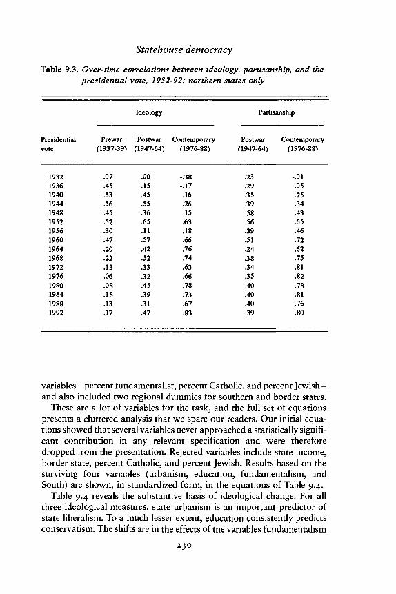
Statehouse democracy
Table 9.3. Over-time correlations between ideology, partisanship, and thepresidential vote, 1932-92: northern states only
Presidentialvote
1932193619401944194819521956196019641968197219761980198419881992
Prewar(1937-39)
.07
.45
.53
.56
.45
.52
.30
.47
.20
.22
.13
.06
.08
.18
.13
.17
Ideology
Postwar(1947-64)
.00
.15
.45
.55
.36
.65
.11
.57
.42
.52
.33
.32
.45
.39
.31
.47
Contemporary(1976-88)
-.38-.17.16.26.15.63.18.66.16.74.63.66.78.73.67.83
Partisanship
Postwar(1947-64)
.23
.29
.35
.39
.58
.56
.39
.51
.24
.38
.34
.35
.40
.40
.40
.39
Contemporary(1976-88)
-.01.05.25.34.43.65.46.72.62.75.81.82.78.81.76.80
variables - percent fundamentalist, percent Catholic, and percent Jewish -and also included two regional dummies for southern and border states.
These are a lot of variables for the task, and the full set of equationspresents a cluttered analysis that we spare our readers. Our initial equa-tions showed that several variables never approached a statistically signifi-cant contribution in any relevant specification and were thereforedropped from the presentation. Rejected variables include state income,border state, percent Catholic, and percent Jewish. Results based on thesurviving four variables (urbanism, education, fundamentalism, andSouth) are shown, in standardized form, in the equations of Table 9.4.
Table 9.4 reveals the substantive basis of ideological change. For allthree ideological measures, state urbanism is an important predictor ofstate liberalism. To a much lesser extent, education consistently predictsconservatism. The shifts are in the effects of the variables fundamentalism
230
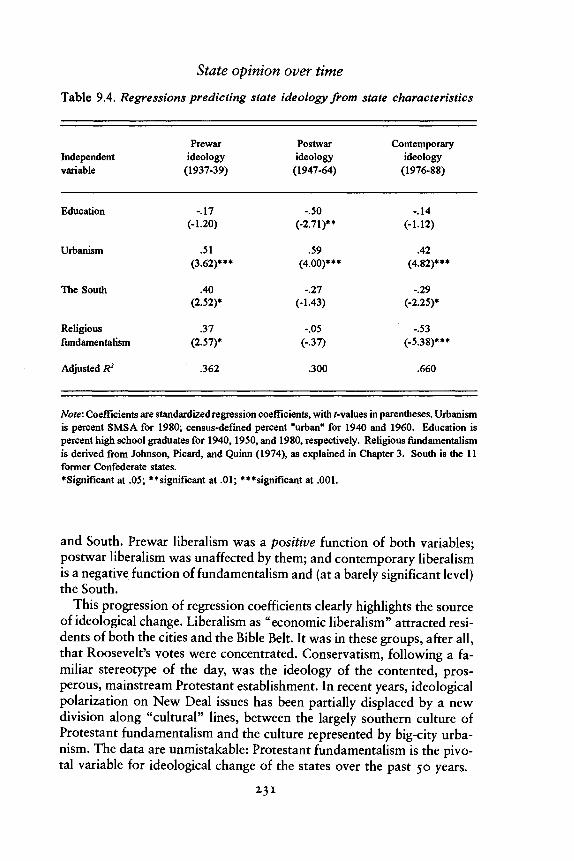
State opinion over time
Table 9.4. Regressions predicting state ideology from state characteristics
Independentvariable
Education
Urbanism
The South
Religiousfundamentalism
Adjusted R2
Prewarideology
(1937-39)
-.17(-1.20)
.51(3.62)***
.40(2.52)*
.37(2.57)*
.362
Postwarideology
(1947-64)
-.50(-2.71)**
.59(4.00)***
-.27(-1.43)
-.05(-.37)
.300
Contemporaryideology
(1976-88)
-.14(-1.12)
.42(4.82)***
-.29(-2.25)*
-.53(-5.38)***
.660
Note: Coefficients are standardized regression coefficients, with t-values in parentheses. Urbanismis percent SMS A for 1980; census-defined percent "urban" for 1940 and 1960. Education ispercent high school graduates for 1940,1950, and 1980, respectively. Religious fundamentalismis derived from Johnson, Picard, and Quinn (1974), as explained in Chapter 3. South is the 11former Confederate states.*Significant at .05; **significant at .01; ***significant at .001.
and South. Prewar liberalism was a positive function of both variables;postwar liberalism was unaffected by them; and contemporary liberalismis a negative function of fundamentalism and (at a barely significant level)the South.
This progression of regression coefficients clearly highlights the sourceof ideological change. Liberalism as "economic liberalism" attracted resi-dents of both the cities and the Bible Belt. It was in these groups, after all,that Roosevelt's votes were concentrated. Conservatism, following a fa-miliar stereotype of the day, was the ideology of the contented, pros-perous, mainstream Protestant establishment. In recent years, ideologicalpolarization on New Deal issues has been partially displaced by a newdivision along "cultural" lines, between the largely southern culture ofProtestant fundamentalism and the culture represented by big-city urba-nism. The data are unmistakable: Protestant fundamentalism is the pivo-tal variable for ideological change of the states over the past 50 years.
231

Statehouse democracy
STATE IDEOLOGY AND STATE POLICY IN HISTORICALCONTEXT
Our resurrection of state ideology from earlier eras would not be completewithout trying to correlate it to policy measures from the same eras. Sim-ply put, does ideological liberalism correlate with policy liberalism in ear-lier times as it has recently? To answer this question, we need to identifyacceptable measures of policy liberalism for earlier decades.
Measuring policy liberalism historically
In Chapter 4, we presented a general measure of state policy liberalism forthe late 1970s and early 1980s, with components drawn from the contem-porary debate among liberals and conservatives. The eight components ofpolicy liberalism, circa 1980, concerned taxation, education, criminal jus-tice, welfare, health care, gambling, consumerism, and women's rights.Ideally, we would simply replicate these measures for earlier eras. Not allof these contemporary policies were the subject of controversy duringearlier historical periods. For example, little variation exists historically instate policies regarding gambling, consumerism, and women's rights.
Given the limited variations of some policies (and the limited historicalinformation about others), we generate a new state policy measure basedon policies that exhibit some readily identifiable variation and com-parability over the past 50 years. This new measure is our index ofwelfare/education spending, constructed from the following four items:
per pupil spending for education,mean teacher salaries,per recipient monthly AFDC [ADC] payment, andper recipient monthly general assistance.
Measures of each were collected for each census year, 1940 to 1990.5
Factor analyses of these four items yield a dominant first factor that ex-plains about 50 percent of the variance in these items for each census year.For each year, we construct the composite index by summing the stan-dardized scores for the four items for that year.
Table 9.5 summarizes the stability of our state spending measure overtime. As we expect from earlier literature (Sharkansky, 1968), we obtainvery high over-time correlations, meaning that the relative positions of thestates on this spending index have changed little over the decades. Notethat these correlations are not indicators of absolute stability - substantialchanges have occurred as a function of inflation and federal government
5. For 1990, the latest available data is actually for 1988 or 1989. For 1990, per capitageneral assistance spending was unavailable. We replaced it by doubling the weightof the mean AFDC payment.
232

State opinion over time
Table 9.5. Over-time correlations for the index of welfare/educationspending
Welfare/educationspending
1940
1950
1960
1970
1980
1990
1940
1.00
.92
.92
.88
.88
.83
1950
1.00
.96
.87
.90
.79
1960
1.00
.93
.94
.85
1970
1.00
.94
.92
1980
1.00
.90
1990
1.00
Note: N =47 states; Alaska, Hawaii, and Nevada are excluded.
intervention if nothing else. But the policy positions of the states relativeto one another have changed very little over the passage of half a century.We can validate the index of welfare/education spending from the correla-tion between the 1980 version of this measure and our original compositemeasure of policy liberalism, for the period centered around 1980. Thiscorrelation is a rather satisfactory .84. (Of course, a high correlationshould be expected if for no other reason than that the two indices shareone item - per pupil spending - in common.) A second validation is thatthe 1980 index of welfare/education spending correlates at .73 with thecontemporary measure of state ideology.
The opinion-policy correlation historically
Table 9.6 shows the simple correlation coefficients between welfare/education spending for each of six decades, on the one hand, and all threereadings of state ideology, on the other. The numbers are presented threeways. The top set represents the correlations for 47 states. The middle setis for 30 northern states. The bottom set is for the 12 largest northernstates. Looking at the top set, we find that contemporary ideology is aboutas strongly related to welfare/education spending going back to 1940 as it
233

Statehouse democracy
Table 9.6. Correlations between state ideology and welfare/educationspending, 1940-90
Welfare/educationspending
47 states
194019501960197019801990
30 northern states
194019501960197019801990
12 largest northern states
194019501960197019801990
Prewar
-.05-.14-.13-.06-.04-.07
.62
.58
.53
.47
.55
.42
.71
.61
.72
.64
.75
.70
State ideology
Postwar
.41
.37
.37
.41
.42
.44
.61
.51
.56
.52
.55
.51
.73
.81
.89
.82
.80
.57
Contemporary
.66
.62
.67
.76
.73
.81
.60
.58
.69
.78
.72
.83
.77
.81
.70
.74
.74
.78
is to recent 1980-90 spending. This is the pattern one would expect ifboth state ideology and policy were stable (although we know ideology isnot). Postwar liberalism is also related to welfare/education spendingthroughout the time span - but less strongly, a plausible result given itsgreater measurement error. Prewar liberalism presents a different result.As measured for the late 1930s, liberal sentiment does not correlate at allwith liberal spending, even for 1940. This result, certainly not attributable
234

State opinion over time
to measurement error, goes against our theoretical expectations aboutrepresentative democracy. Did something go wrong?
Actually, there is a ready explanation in terms of the one-time politicaluniqueness in the U.S. South. Figure 9.5 displays the scatterplots of theideology-spending correlations for 1940, i960, and 1980, in each in-stance using the temporally closest measure of state ideology. Southernand border states are highlighted as solid dots in the graphs. Over time,the southern scatterplot has begun to approximate the North's. For 1940,however, the North and South diverged dramatically. The dominant fea-ture of the 1940 graph is the clustering of southern states in the lower rightcorner, a location indicating relatively conservative spending policiescombined with a plurality of liberals over conservatives in the electorate.This mismatch of ideology and policy in the South easily accounts for thenoncorrelation for 1940 between prewar ideology and policy nationally.
But if southern opinion was so "liberal," why was southern policy moreconservative?6 Again, we turn to V. O. Key. Key believed that the liberal-ism of the southern electorate was thwarted by the structure of the politi-cal system that permitted economic conservatives to prevail over otherinterests by fanning the flames of racial antagonism. Economic conserva-tives, in control of policy making in the states of the Old South, restrainedthe expansion of state governments. The task was eased by an unrespon-sive one-party system. In Key's words, "An underlying liberal drive . . . isheld in check in part by the one-party system which almost inevitablyoperates to weaken the political strength of those disposed by tempera-ment and interest to follow a progressive line" (1949, 670).
With time, the South discovered the two-party system and acceptedblack suffrage. Along the way, state ideology and state policy becamemore congruent, but not - as Key had predicted - by the adopting ofliberal policies. Instead, ideology became conservative to match policy.The impetus, of course, was the new urgency in the 1950s of racial policyas the defining issue of southern politics. The white South rediscovered"states rights" and the virtues of "limited government." In more recentyears, the dominance of conservatism as the preferred label in the Southhas been aided by the new ideological polarization along cultural lines.The dominance of conservatism in the South became complete. (See Blackand Black, 1988, for a thorough discussion.)
For northern states, the analysis of the ideology-spending relationshipis not so complicated. Compared to southern and border states, northernstates were less affected by changing meanings of "liberal" and "conser-vative" in terms of race and culture. Northern states were not preoccupied
6. Actually, prewar ideology and 1940 spending are correlated for the South andborder states, but in the wrong direction, -.65.
235

2-
o-
-2
'408 Spending by Prewar Ideology
o
°oo
°° s° *
0
•
•
o
o0
%
•
•
•
•
-40 -20 20
O)
ICO
s
'60s Spending byPostwar Ideology
* • • :
-40 -20 20
-2"
'80s Spending byContemporaryIdeology
-40 -20 0
State Ideology
20
Figure 9.5 Ideology-Spending Relationship OverTime. Note: Solid dots = southern and border states.

State opinion over time
by battles over voting rights and desegregation, nor did they undergo atransformation from one-party to two-party politics. For the remainder ofour analysis of the ideology-policy connection, we will concentrate onour set of 30 northern states.
The Table 9.6 correlations for 30 northern states are all positive, withopinion liberalism at each of three periods predicting policy at all fivereadings. The same is true of correlations for the 12 largest northernstates, with the correlations involving the pre- and postwar measures im-proving considerably. This is because restricting the sample to large statesdiminishes the threat of measurement error.
State income
So far we have ignored one important complication. Since our historicalpolicy measure represents the degree of liberal spending, this variable isinfluenced by state wealth as well as ideology. Although state wealth maynot have much of an independent effect on policy liberalism in general (seeChapter 4), rich states do spend more than poor states, in part for thereason that they can afford it. Indeed, for our 30 northern states, theaverage decennial state spending-state income correlation is a rather im-posing .80. For complex reasons, state income also correlates with opin-ion liberalism.7 Clearly we should check whether the observed ideology-spending correlations are "spurious" due to both variables correlatingwith income. Therefore, controlling for state income is in order. However,when both state ideology and state wealth compete within the same equa-tion, state ideology is disadvantaged by its measurement error. One doesnot know for sure how much the independent "effect" of state incomeactually reflects an income effect and how much it represents stateideology.8
Table 9.7 presents the multivariate welfare/education spending equa-tions, 1940 to 1990, for 30 northern states. Spending is predicted as afunction of per capita income at the time plus each measure of state opin-ion liberalism, entered separately.9 Look first at the equations predicting1980 and 1990 spending from 1980 income and contemporary state ide-
7. Wealthy states are liberal largely because urbanism makes a state wealthy and urban-ism attracts liberals. See Chapter 3. Urbanism does not show an independent effecton state spending, once state income is taken into account.
8. One bit of evidence that income stands for liberalism is that the contemporarymeasure of state ideology is more strongly correlated with state income, both pastand present, than are the more error-prone historical measures. Also, the historicalmeasures of ideology become increasingly correlated with income when smallerstates are culled.
9. We employ per capita income here instead of median income, because only percapita income is available for all six decades of our analysis. For 1990, the measureof per capita income is actually for 1988.
2-37

Statehouse democracy
Table 9.7. Regressing state welfare/education spending on state incomeand state ideology, 1940-90, for 30 northern states
Welfare/educationspending
1940
1950
1960
1970
1980
1990
Per capitaincome
.78***
.84***
.99***
.66***
.67***
.70***
.76***
.76***
.76***
.79***
.80***
.64***
.56***
.57***
.35*
.75***
.73***
.39*
Prewar
.26**
.32**
.25*
.19
.37**
.22
State Ideology
Postwar
.07
.32**
.18
.10
.33*
.15
Contemporary
.12
.13
.13
.29*
.51**
.53**
AdjustedR2
.830
.776
.777
.685
.681
.600
.758
.729
.709
.749
.721
.749
.542
.514
.598
.666
.638
.735
Note: Per capita income is measured for the census year of the spending measure. Coefficientsare standardized regression coefficients.•Significant at .05; **significant at .01; ***significant at .001 level.
ology. Since it contains little error, our measure of contemporary ideologydominates state income as a predictor of 1980 and 1990 welfare/education spending, although both ideology and income are statisticallysignificant. For all other comparisons, state income is the dominant vari-able, but the effect of ideology shows through if a timely measure is used.For instance, contemporary state ideology fails to predict earlier spending.Similarly, prewar ideology predicts earlier spending far better than 1980or 1990 spending. In general, the closer together the ideology and the
238

State opinion over time
spending readings are in time, the stronger the ideology "effect." Postwarideology presents the most disappointing performance, but with a timelysignificant "effect" for 1950 spending.
These results hint of an underlying dynamic process, with current stateideology affecting spending both now and, at a decaying rate, in the fu-ture. Coefficients for prewar and postwar ideology are attenuated, how-ever, by the limited quality of the measures. The one best measure ofideology - the contemporary reading - does predict 1980 and 1990 spend-ing at the expense of state wealth as predicted. One can readily imaginethat better ideology measures for other years would also dominate theprediction of liberal spending at the time.
To see the role of ideology come to life when measurement error isabated, we can redo our regressions while restricting the sample to the 12largest northern states. Alternatively, rather than discard cases entirely, wecan "weight" the 30 northern states by their sample sizes. Table 9.8displays the results for these two regressions. The most timely measure ofideology and state income are entered as predictors of welfare/educationspending at our six decade readings.
With states weighted by their sample sizes, the standardized regressioncoefficients give the statistical edge to ideology over income, even for thehistorical pre-1980 regressions. When the 12 largest northern states areconsidered together, unweighted, this edge becomes clearer. For all butone equation, for 1940, the better predictor of state spending is the mea-sure of state ideological sentiment.
The causal connection
Our historical analysis relies on a policy measure that reflects policy some-what narrowly in terms of liberal spending. Measuring policy in terms ofspending has been the typical practice of state policy analyses (e.g., Dye,1966; Sharkansky, 1968; Hofferbert, 1974). Past studies have rightly mar-veled at the degree to which spending variables correlate with statewealth. It is no wonder that these earlier studies focused on state economicdevelopment as perhaps the leading cause of state policies.
What these earlier studies lacked was any direct measure - no matterhow weak - of state public opinion. Suppose earlier authors had rigged upsome measure of state ideology from Gallup polls like we have done.Suppose also that they had related this measure to measures of liberalspending as we have, with appropriate statistical controls. A straighfor-ward regression of environmental variables along with a weak publicopinion measure, based on all the states, would not have revealed anyimportant role for state ideology in the policy process.
To uncover the rather important role of public opinion in these earlier
239

Statehouse democracy
Table 9.8. State ideology sample size and the welfare/education spendingregressions, 1940-90
Welfare/educationspending
1940 spending,prewarideology
1950 spending,combined pre-,postwar ideo.
1960 spending,postwarideology
1970 spending,postwarideology
1980 spending,contemporaryideology
1990 spending,contemporaryideology
30 Northern states,weighted by sample size
Income
.67***
.48***
.64***
.60***
.11
.27
Ideology
.34***
.51***
.33**
.31*
.67***
.60**
Adjusted R2
.529
.786
.797
.693
.549
.664
12 Largest northernstates, unweighted
Income
.68***
.48*
.35
.39
.17
-.13
Ideology Adjusted R2
.41* .848
.52* .741
.61* .775
.56* .701
.59 .415
.89* .583
Note: Per capita income is measured for the census year of the spending measure. Coefficientsare standardized regression coefficients.•Significant at .05; **significant at .01; ***significant at .001 level.
years required that we had a clear idea of what we were looking for. In thischapter, we have found an important role for state ideology, but to do so,we needed to incorporate rather massive sectional changes in ideologicalattachments and were compelled to respect the mischief of measurementerror. Particularly, as we culled southern states and then small states, wefound considerable evidence that state opinion mattered for the decadesprior to 1980. In staking this historical claim, our path was illuminated bythe experience of our search for the contemporary period, which under
240

State opinion over time
favorable measurement conditions found clear evidence of a strong stateideology-policy connection. On theoretical grounds, it would seem quitelikely that if state ideology mattered for one particular time, it would alsomatter for others.
In conducting this historical search, one hope was to find some clue tothe dynamics of policy change. As we measured it in terms of liberalspending, relative positions of the states remained remarkably stable overthe decades - as did their easiest predictor, state income. Although weemphasized the fact of change, state ideology also showed a stable compo-nent, once the twists of how southern and border state residents relate toideological labels were taken into account. Thus, the configuration of thestate opinion-policy relationship changes little on a decade-to-decadebasis. Still, the data show hints of evolutionary cause and effect. As theSouth yielded its preoccupation with the politics of racial segregation andbegan to approximate two-party politics, southern and border statesedged toward the democratic practice of enjoying policies that reflectpublic preferences. Also, we see evidence, clear in outline but dim in spe-cifics, that when states change ideologically, policy change may result infairly short order. State governments respond to state preferences todaymore than to preferences in decades past.
2 4 1

Appendix: Historical question wordingvariations Gallup poll, (1937-64)
Ideology: Party referent
A. If there were only two political parties in this country, one for conserva-tives and one for liberals, which would you join?
AIPO37-OO69B. If there were only two political parties in this country, one for conserva-tives and one for liberals, which do you think you would join?
AIPO38 -0127C. If these two new parties (one for conservatives and one for liberals)were formed, which one do you think you would join?
AIPO37 - 0094D. Which party (one for conservatives and one for liberals) do you thinkyou would like to join?
AIPO38-OI18E. If the Democratic and Republican parties went out of existence, wouldyou join the Conservative or the Liberal Party?
AIPO38-O132R If our political parties were reorganized and there was one for conserva-tives and the other for liberals, which party do you think you would like tojoin?
AIPO48 - 0421G. Suppose there were only two major parties in the United States, one forliberals and one for conservatives, which would you be most likely toprefer?
AIPO6o - 0630AIPO61 - 0649AIPO62 - 0665AIPO63 - 0677AIPO64 - 0694AIPO64 - 0702
242

State opinion over time
Ideology: Self-identification
A. In politics do you regard yourself as a liberal or conservative?AIPO38-OIO9
B. In politics, do you consider yourself a radical, a liberal or aconservative?
AIPO39-O161 (Form A)C. In politics, do you consider yourself a conservative, a liberal or a radi-cal?
AIPO39 - 0161 (FormB)D. Do you consider yourself to be a conservative or a liberal in yourpolitical views?
AIPO46-O387E. Taking everything into account, would you say that, in general, youthink yourself as a liberal or as a conservative?
AIPO55-O547AIPO57 - 0577
Party identification
A. In politics, as of today, do you consider yourself a Republican,Democrat, Socialist, or Independent?
AIPO46-O387AIPO48 - 0421
B. In politics, as of today, do you consider yourself a Republican,Democrat, or Independent?
AIPO54 - 0527AIPO54 - 0541AIPO55-O547AIPO57 - 0577AIPO61 - 0649AIPO62 - 0665AIPO63 - 0677AIPO64 - 0694AIPO64 - 0702
243

1O
Conclusions: Democracy in the Americanstates
This book has argued that public opinion is the dominant influence onpolicy making in the American states. In this concluding chapter, we sum-marize our evidence for strong democratic representation in the states,place our findings in the context of the behavioral literature on democra-tic politics, and discuss the implications for the understanding of repre-sentative democracy.
Our story depends on the distillation of policy questions to a singledimension of ideology, what is commonly called liberalism-conservatism.Ideology - whether one dimension or many - does not neatly account forall government policies or all public preferences or even keep its precisemeaning from one decade to the next. But the simplification of policy toone ideological dimension provides powerful leverage for understandingthe ideological connection between public preferences and governmentpolicy in the U.S. states. Representation in the states works not necessarilyin terms of government compliance with specific public demands (al-though this assertion is largely untested) but rather in terms of publicopinion controlling the general ideological direction of state policy.
Our project was set in motion by the availability of state-level samplesof ideological preference. Aggregation of opinion from the CBS/NYT sur-veys provided plausible scores for the states in terms of ideological identi-fication plus the important variable of party identification. Given thesample sizes, these measures are highly reliable from a statistical stand-point. Moreover, for the 1976-88 period for which we collected stateopinion data, the ideological orderings of state electorates appear ex-tremely stable. States moved around only slightly on the scale of relativeDemocratic versus Republican partisanship and hardly at all on ideology.This result conveniently allowed us to pool the full accumulated set ofrespondents for the 1976-88 period without fear of states changing dra-matically over the time period.
The patterns of ideology and partisanship we find in the states are not
244

Conclusions
simple reflections of the demographics of the states. We find that the stateshave distinct ideological centers of gravity and patterns of partisan attach-ments that are not attributable simply to the social and economic charac-teristics with our respondents. The importance of this finding is that itdemonstrates that states, as political communities, do have values andtraditions that can be measured only with survey research and are explain-able in terms of a shared common political culture. State publics are, in asense, more than the sum of their demographic parts.
Our crucial concern about state-level ideology is the relationship be-tween state opinion and policy. We constructed a policy index composedof eight indicators of the relative liberalism-conservatism of state pol-icies. We found strong observable correlations of .82 for the full set ofstates and a remarkable .94 for the 11 largest states for which measure-ment error is minimal. This result holds up in the face of controls for thesocioeconomic variables that the state policy literature had insisted domi-nate the state policy process. Our evidence shows that the apparent statis-tical power of state socioeconomic variables is largely an illusion.Socioeconomic variables - wealth, education, urbanism - simply reflectthe state public's ideological taste. With ideology taken into account, theymake little statistical contribution.
Had political scientists known in the 1960s and 1970s that their mea-surable socioeconomic variables like state wealth were actually proxies forstate ideology, research on comparative state politics might have gone adifferent direction. In light of our current interpretation, earlier researchon the importance of socioeconomic (or "environmental") variables isconsistent with our claim that state politics does exactly what it is sup-posed to do in theory - faithfully translate public preferences into broadpatterns of policy outcomes.
Parties and elections are the central conduits for mass influence in ourmodel. Our analysis of state party elites illuminates the policy tensionbetween the centrifugal push by party activists toward their "extreme"ideologies and the centripetal pull toward the center by the more moder-ate electorate. The ideological orientations of state-level political partiesare jointly explained by their two, often conflicting constituencies: partyactivists and the general electorate.
Party positions affect elections largely via their cumulative influence onthe state electorate's party identification. In each state, most voters see theDemocrats to their left and the Republicans to their right. Voters respondin Downsian fashion to the parties' proximities to the voters' own ideo-logical preferences. Operationally, when the two parties are too liberal forthe average voter, the Republican Party gains identifiers; when the partiesare too conservative, the Democrats gain.
State partisanship matters considerably in state politics because it is the
245

Statehouse democracy
dominant cause of the parties' relative strengths in the state legislature.State partisanship influences gubernatorial elections too, but to a far lesserdegree. Gubernatorial election outcomes start with the normal vote base-line from state partisanship, but they are strongly influenced by the idio-syncratic issues of the specific campaigns.
It is important to note that state-level party identification is not simply afunction of the state electorate's liberalism or conservatism. Instead, statepartisanship depends on the relative approximation of the two state partypositions to the electorate's mean preference on the ideological con-tinuum. This dependence is revealed by the way state partisanship corre-lates with state-level voting for president, for which the relevant partypositions are nationally fixed rather than variable by state. Where statepartisanship is skewed Republican by overly liberal parties, presidentialvoting is more Democratic than one would expect; where state partisan-ship is skewed Democratic by overly conservative parties, presidentialvoting is more Republican than one would expect. State partisanship ap-pears to fully incorporate state ideology as well as state party positions:When party positions and state partisanship are controlled, state ideologyshows no additional independent effect on state voting at any level.
A key question is whether certain conditions enhance the degree ofdemocratic representation this book describes. Interestingly, the one iden-tifiable variable that statistically divides states in terms of responsivenessis Daniel Elazar's classification of state political subculture as tradi-tionalistic, individualistic, or moralistic. We find the lowest responsive-ness of policy to opinion in the traditionalistic (largely southern) statesand the highest responsiveness in the individualistic states, where the pol-icy process appears driven by the parties' willingness to accommodatestate opinion over activist ideology. For parties in individualistic states,winning seems to dominate ideology. Moralistic states, on the other hand,show parties driven more by their own ideological concerns than by elec-toral necessity. In moralistic states, the ideological distances between theparties are greater, and legislators appear more faithful to their party pro-grams.
We also investigated whether representation varies across time. Analy-sis of a collection of Gallup polls from the 1930s to the present revealedconsiderable change in state electorates' ideologies over the decades, par-ticularly in the South. The meaning of the liberal-conservativedistinction - although never precise - evolves over the years with the issuesof national politics and the labels elites use to identify their positions onthose issues. Southerners, in particular, changed from being relatively lib-eral before World War II to now quite conservative. This shift was broughtabout by the intrusion first of race onto the agenda of U.S. politics and
246

Conclusions
then by the more recent social agenda of concerns such as abortion rights,life styles, and law and order.
The most important aspect of our historical investigation is to showthat state policy responsiveness is not unique to the 1970s or 1980s.Stretching back to before World War II - and here we stretched our dataresources to the limit - we uncovered ample evidence of the opinion-policy connection in the states. When opinion changes (which is not oftenor much), policy does seem to follow.
Ultimately, our message about representation in the states is a simpleone. At the ballot box, state electorates hold a strong control over theideological direction of policies in their states. In anticipation of this elec-toral monitoring, state legislatures and other policymakers take publicopinion into account when enacting state policy. These means of controlare uncertain in any particular application but accumulate to create astriking correlation between the mean ideological preference of state elec-torates and the mean ideological tendency of state policy.
THE PUZZLE OF REPRESENTATION
The process we describe places responsibility for ideological direction onthe shoulders of state electorates. Somehow, state electorates are up forthis task. The puzzle is how they exert their control, given what modernpolitical science knows about the limitations of individual voters. Let usbriefly review the evidence regarding ideology and the U.S. voter.
Much of what we know about U.S. voters comes from the unfavorableportrait presented by Campbell, Converse, Miller, and Stokes in TheAmerican Voter (i960) and subsequent work. In the first detailed study ofthe presidential voters at the national level, The American Voter foundthat few Americans were motivated by policy issues or used the spatialmap of the Left-Right ideological continuum for political guidance. Theydescribed a largely nonideological electorate that gave shockingly littleattention to the policy issues of the campaign, voting largely as a functionof long-ingrained party identifications plus reactions to candidate per-sonalities (Campbell et al., i960). When they looked for the informationalbasis for representation in congressional elections, Stokes and Miller(1966) found little there either; voters in congressional elections werewoefully ill informed. Their findings of citizen ignorance about the policypositions of their congressional candidates became a benchmark docu-menting citizen failure to meet the apparent standards expected bydemocratic theory. Perhaps most devastating of all was the discovery thatperhaps a meaningful public opinion did not even exist. In an importantand influential paper, Converse (1964) argued that a substantial portion of
247

Statehouse democracy
the public responses to survey questions about the issues of the day arereally "nonattitudes." And thinking about politics ideologically - so com-mon among political elites - was nearly absent for the mass public. WhileConverse's work stirred up considerable controversy, it remains difficult,based on the evidence, to challenge the accuracy of his general portrait ofthe average citizen as someone with little interest in or information aboutpolitics.
Subsequent survey research suggests a greater public facility with theideological language of liberalism versus conservatism and a greaterdegree of ideologically motivated voting than The American Voter au-thors were initially willing to credit. But even taking into account theupdated evidence, ideology activates no more than a minority even in themost heated of campaigns (see, e.g., Nie, Verba, and Petrocik, 1979;Knight, 1985). And no evidence has surfaced to doubt The AmericanVoter's general portrait of an inattentive electorate. In terms of the strongexpectations of democratic theory, the accumulation of evidence fromsurvey research only reinforces the now familiar image of the averagevoter as inadequate for the task assigned by democratic theory: to serve asthe engine of representative democracy.
Our special challenge is to reconcile the limited political capabilities ofindividual citizens, which we know from survey research, with the stronglinkage between state electorates' ideological preferences and the ideolog-ical direction of their states' policies. How can voters who are individuallyuninformed and inactive manage collectively to achieve such levels ofpolicy responsiveness from government? One's initial assumption is likelyto be that if most individuals are inattentive, poorly informed, and givento vote on the basis of image and candidate familiarity rather than onissues, then the quality of collective decisions must be similarly im-poverished. But this pessimistic conclusion does not follow. The correctanswer is that the quality of an electorate's collective decision can begreater than the individual decision processes of the citizens who make upthe electorate. Let us examine how this happens.
With his "jury theorem," Condorcet (1785) was the first to articulatethe powers of aggregation in the electoral context. When individuals holddisparate beliefs regarding some truth, most individual perceptions mustnecessarily be incorrect. Yet under plausible conditions, as a group theseindividuals will arrive at the appropriate answer with remarkable con-sistency (Feld and Grofman, 1988; Grofman and Owen, 1986; Miller,1986). They do so because errors cancel out. In this way, the collectivepolitical intelligence and attentiveness of an electorate can exceed thatwhich one would infer from knowledge of individuals' survey responses.
One context in which this process can be clearly seen is the public'sevaluation of economic performance. Consider the contrast between the
248

Conclusions
macrolevel and microlevel analysis of economic conditions and votingbehavior. At the macrolevel, when they vote or even pass judgment on thepresident's performance, the citizenry responds rationally and predictablyto even relatively slight changes in the economy. On the other hand, themicrobases for such clear aggregate patterns are obscure and difficult tofind. Perceptions of the economy, generally accurate in the aggregate, arewoefully ignorant among individuals (Conover, Feldman, and Knight,1987).
Consider the contrast between the macrolevel and microlevel analysisof policy representation in Congress. Studies of congressional voters showthat individuals are generally vague at best regarding the ideological rec-ord of their congressmember or senator. One might infer, then, that wherecongressional candidates stand ideologically has little bearing on theirelectoral success. However, as errors cancel at the macrolevel, constituen-cies' mean perception of representative ideology correlates quite stronglywith objective measures of representative ideology, such as the ratings byideological groups (Erikson, 1981, 1990). The result is that constituency-level congressional elections are often decided by the relative ideologicalproximity of candidates to constituencies (Erikson and Wright, 1980,1993)-
Impressive also is the evidence from experimental studies of voting un-der various degrees of voter information (McKelvey and Ordeshook 1986,1990). Deficiencies in information do very little to affect electoral out-comes. Well-informed and poorly informed experimental electorates ap-pear to make about the same kinds of collective decisions, eachapproximating the Downsian outcome of selecting the more proximatecandidate, where that criterion is applicable.
The lesson is an important one. What we learn about individuals interms of their lack of political sophistication does not apply fully to elec-torates. Lack of political concern within the citizenry does not mean poli-ticians can treat electorates as though voters are fools. That many peoplecannot articulate their detailed issue preferences and cannot report accu-rately where their elected officials stand on issues does not mean thatlegislators can do whatever they want in the policy arena. Public opinionas an entity is a more sophisticated, stable, and reasonable force than wecould ever guess from looking at the political attitudes and knowledge ofindividual citizens.
The key is what Converse (1990, 383) termed the "miracle of aggrega-tion." When we aggregate across individual respondents identified bysocially heterogeneous characteristics, such as social class, regions, race,religion, or for us, the state of residence, response patterns of the aggre-gate are more clearly defined and generally better behaved than are theirindividual-level counterparts. As measured in surveys, one finds consider-
249

Statehouse democracy
able noise in the measurement of individual ideology positions or - evenharder - perceptions of the ideological positions of political actors orpolitical parties. They contain errors due to genuine individual confusion,idiosyncratic interpretations of the questions, the context of the interview(both in its immediate surroundings and in the larger sociopolitical con-text of the moment), and other sources. This individual error, which oftendominates in analyses of survey data, cancels out in the aggregation pro-cess. We may consider any response to a survey being constituted by twoparts: the real signal and noise, which is error from such multiple potentialsources as those just mentioned. With individual data, the signal-to-noiseratio is frequently very low, so much so that analysts frequently see noiseas the dominant feature of the survey response. At the macrolevel, thisrandom noise cancels out so that upon aggregation the signal-to-noiseratio is much more favorable.
The idea is simple but important. Because people have some idea oftheir interests and some idea of where candidates and the parties stand, asa group they can make much "better" decisions than they do as individu-als. Even when many citizens mistakenly vote for the "wrong" candidate(in the sense that with a lot more information and study, they would votedifferently), such errors will tend to cancel out so that in the end the fullelectorate will often behave very much, although not exactly, as it wouldhave had individuals had much better information and were less errorprone in their decision making.
We do not want to overstate the powers of aggregation here. It remainsentirely possible for politicians to successfully misrepresent themselves tomajorities of the electorate. Aggregation will mitigate the problems due toidiosyncratic or random error in voter perceptions and decisions, but itdoes not lessen the effects of effective and deceptive appeals to voters'values. The only protection here is that elections are periodic and theelectorate can therefore change its decisions. Thus, even if occasionallymistaken, public opinion remains important, indeed vital, as long as wecan assume that "you cannot fool all the people all the time."
Aggregation gain
In the process we describe, aggregation works to connect state opinion tostate policy, with both variables condensed to a point in a single dimensionof ideological space. So far, the gain from aggregation is restricted to thesignal that comes through when preferences, perceptions, or votes aremeasured at the group rather than individual level. For the study of repre-sentation in the states, we profit from additional aggregation processes aswell.Aggregating over issue preferences. Implicitly, one's net ideological prefer-ence is an aggregation over a variety of concerns. When asked whether
250
Conclusions
they are liberal, moderate, or conservative, respondents must take intoaccount their positions across numerous issues, as well as affective reac-tions to groups and ideologically known leaders (Conover and Feldman,1981; Carmines and Kuklinski, 1990). Thus, self-identified ideology isalready a summary response, and studies frequently find individual votechoices are more strongly related to this summary measure than to specificissues.Aggregating over time. We also aggregate over time. If there are tem-porally fluctuating aspects to ideological self-identification, these wouldtend to cancel out for our state electorates in our summary measure. Theclarity of issue choices in an election does influence the impact of ideology,and this, of course, varies over time and across campaigns (Page, 1978;Nie, Verba, and Petrocik, 1979; Wright and Berkman, 1986). This ag-gregation over time should help to even out short-term variations in un-derlying state ideological preferences.Aggregating over constituencies. Our analysis also entails a tremendousaggregation over constituencies. For a study of dyadic representation (therelationship between the legislator and his or her district), it is most ap-propriate to sample opinion at the district level. Of course, our respon-dents are sampled and aggregated to the state level, not at the level of theindividual state legislative district. This process squeezes additional noiseout of the representational relationship. Certainly, if we could measure theprocess accurately, we would find that more liberal state legislativedistricts manage to elect, on average, more liberal state legislators. Such arelationship becomes even stronger when aggregated to the state level, asit has been here, than if we had investigated the same relationship at thedistrict level. The "errors" of representation with some state legislatorsbeing too liberal and others somewhat too conservative for their districtsshould tend to cancel out across a full legislature, so that the whole is morerepresentative than the individual parts.Aggregation across policy outcomes. Finally, we have aggregated acrosspolicies. Our main analysis has examined our composite measure of statepolicy liberalism, which is made of up eight different state policies. Theoverall index tends to perform better in our analysis than do the individualcomponents, although each of them bears a modest relationship with stateopinion.
It takes these multiple aggregations to obtain the evidence of a strongideological connection between opinion and policy in the states, plus theevidence of the partisan and electoral behavior that produces it. The argu-ment is not that public opinion always triumphs or anything close to that.We argue instead that when it comes to the general ideological direction ofa state's policy making, the ideological preferences of the state electorate isthe dominant guiding force. Put another way, the simple logic of democra-
251

Statehouse democracy
tic electoral politics constrains the ideological tendency of state policy tostay within the fairly narrow channels defined by the state public's specificideological tastes.
DEMOCRACY AND REPRESENTATION IN THE STATES
Public opinion, as it operates in the political arena, is a collective, not anindividual, phenomena. Democratic theorists often write of public opin-ion as a collective entity - of the "will of the people" or the reactions of"the public" to new political events. With the availability of a wealth ofsurvey data, political scientists, however, have generally addressed ques-tions about public opinion by trying to explain individual opinion forma-tion and change rather than by making "electorates" their units ofanalysis. An unfortunate by-product of this emphasis on the individualover the aggregate has been the disconnection of the study of mass be-havior from the larger body of democratic theory and from the study ofpolitical institutions and policy making. Scholars who study the individualcitizen often describe the typical voter as unfit for the job prescribed byversions of democratic theory that stress popular control of government.As we have pointed out, the dynamics and properties of collective opinionare fundamentally different from those of individual opinion. For citizensas a group, opinion is better informed, more perceptive, and more stablethan for individuals. Moreover, forces that move collective opinion inunmistakable ways at the macrolevel are often but a faint whisper, all butinaudible in the noisy data of individual-level survey responses.
Let us add a caveat here so that we do not overstate our argument. Wesee public opinion in much the same way as V. O. Key (1961, chap. 21)when he wrote about public preferences forming "opinion dikes" withinwhich activists and elected officials may act. Public opinion, in this per-spective, seldom "demands" much, nor does it speak with a clear voice.Rather, it sets the boundaries that rational politicians seek to learn andthen heed. Within these dikes, or areas of discretion, many of the morevisible aspects of day-to-day political life in the states have their influence.Party and electoral elites work to define agendas and define issues; interestgroups work for leverage and favor; and the major presence of the nation-al government with its imposing rules and constraints limits the optionsand offers opportunities in many policy areas.
We do not assert that policy making in the states is determined by stateopinion exclusively or with unerring fidelity. Only the most naive versionof democratic theory would argue for such a simple equation betweencitizen preferences and government action. Our claim is more modest: Weassert that public opinion does have a strong influence on general patternsof state policy - the correspondence is strong, but we do not claim anyone-to-one fidelity.
252

Conclusions
In our view, the appropriate message is that even under adverse condi-tions such as the limited interest and information that the average voterhas regarding state politics, public opinion can be observed to influencestate policy. This statement is cautiously worded, but it presents an op-timistic message. If public opinion matters under adverse conditions, cer-tainly it could influence policy even more if state publics were givengreater informational opportunities. We may also speculate that a moreinformed public would be more cognizant of its political interest. If evenweakly informed state publics influence policy, one can imagine the pro-gress in state-level democracy if citizens were more fully capable of per-forming the task of governing that is assigned them by democratic theory.
253

References
Abramowitz, Alan I. 1988. "Explaining Senate Elections Outcomes." AmericanPolitical Science Review 82: 385-403.
Aldrich, John H. 1983. "A Downsian Spatial Model with Party Activism." Ameri-can Political Science Review 77: 974-90.
Almond, Gabriel, and Sidney Verba. 1963. The Civic Culture: Political Attitudesand Democracy in Five Nations. Princeton, N.J.: Princeton University Press.
Alt, James E. 1985. "Political Parties, World Demand, and Unemployment:Domestic and International Sources of Economic Activity." American PoliticalScience Review 79: 1016-40.
Backstrom, Charles H. 1977. "Congress and the Public: How Representative IsOne of the Other?" American Politics Quarterly 5:411-35.
Baer, Denise L., and David A. Bositis. 1988. Elite Cadres and Party Coalitions:Representing the Public in Party Politics. New York: Greenwood.
Beck, Nathaniel. 1982. "Parties, Administrations, and American MacroeconomicOutcomes." American Political Science Review 76: 83-93.
Black, Earl, and Merle Black. 1988. Politics and Society in the South. Cambridge,Mass.: Harvard University Press, 1987.
Black, Merle, David M. Kovenock, and William C. Reynolds. 1974. Political Atti-tudes in the Nation and the States. Chapel Hill, N.C.: Institute for Research inthe Social Science.
Boles, Janet K. 1979. The Politics of the Equal Rights Amendment. New York:Longman.
Brady, David W. 1988. Critical Elections and Congressional Policymaking. Stan-ford, Calif.: Stanford University Press.
Browning, Robert X. 1985. "Presidents, Congress, and Policy Outcomes: U.S.Social Welfare Expenditures, 1949-1977." American Journal of Political Sci-ence 29: 197-216.
Browning, Robert X., and William R. Shaffer. 1987. "Leaders and Followers in aStrong Party State." American Politics Quarterly 15: 87-106.
Bullock, Charles S., and David W. Brady. 1983. "Party, Constituency, and Roll-Call Voting in the U.S. Senate." Legislative Studies Quarterly 8: 29-43.
Burnham, Walter Dean. 1970. Critical Elections and the Mainsprings of AmericanPolitics. New York: Norton.
Burstein, Paul. 1981. "The Sociology of Democratic Politics and Government." InRalph H. Turner and James F. Short, Jr., eds. Annual Review of Sociology, vol.7, pp. 291-319. Palo Alto, Calif.: Annual Reviews, Inc.
2-54

References
Calvert, Randall L. 1985. "Robustness of the Multidimensional Voting Model:Candidate Motivations, Uncertainty and Convergence." American Journal ofPolitical Science 29: 69-95.
Cameron, David C. 1978. "The Expansion of the Public Economy: A ComparativeAnalysis." American Political Science Review 72: 1243-61.
Campbell, Angus. 1966. "Surge and Decline: A Study of Electoral Change." InCampbell et al., Elections and the Political Order, pp. 40-62. New York:Wiley, 1966.
Campbell, Angus, Philip E. Converse, Warren E. Miller, and Donald E. Stokes.i960. The American Voter. New York: Wiley.
1966. Elections and the Political Order. New York: Wiley.Cantril, Hadley. 1951. Public Opinion, 1935-46. Princeton, N.J.: Princeton Uni-
versity Press.Carmines, Edward G., and James H. Kuklinski. 1990. "Incentives, Opportunities,
and the Logic of Public Opinion in American Political Representation." In JohnA. Ferejohn and James H. Kuklinski (eds.), Information and Democratic Pro-cesses, pp. 240-68. Urbana: University of Illinois Press.
Carmines, Edward G., and James A. Stimson. 1989. Issue Evolution: Race and theTransformation of American Politics. Princeton, N.J.: Princeton UniversityPress.
Carmines, Edward G., and Richard A. Zeller. 1979. Reliability and Validity As-sessment. Beverly Hills, Calif.: Sage.
Castles, Francis G. 1982. "Politics and Public Policy." In Francis G. Castles (ed.),The Impact of Parties on Public Expenditures, pp. 21-96. Beverly Hills, Calif.:Sage.
Clubb, Jerome M., William H. Flanigan, and Nancy H. Zingale. 1980. PartisanRealignment: Voters, Parties, and Government in American History. BeverlyHills, Calif.: Sage.
Committee on Political Parties of the American Political Science Association.1950. "Toward a More Responsible Two-Party System." American PoliticalScience Review 44: Supplement.
Condorcet, Marquis de. 1785. Essai sur Vapplication de Vanalyse a la probabilitedes decisions rendues la pluralit des voix. Paris: Imprimerie Royale.
Conover, Pamela J., and Stanley Feldman. 1981. "The Origins and Meaning ofLiberal/Conservative Self-Identifications." American Journal of Political Sci-ence 25: 617-45.
Conover, Pamela J., Stanley Feldman, and Kathleen Knight. 1987. "The Personaland Political Underpinnings of Economic Forecasts." American Journal of Po-litical Science 31: 559-83.
Converse, Jean M., and Howard Schuman. 1984. "The Manner of Inquiry: AnAnalysis of Survey Question Form Across Organizations and Over Time." InC. F. Turner and E. Martin (eds.), Surveying Subjective Phenomena. Vol. 2, pp.283-316. New York: Russell Sage Foundation.
Converse, Philip E. 1964. "The Nature of Belief Systems Among Mass Publics." InDavid Apter (ed.), Ideology and Discontent, pp. 206-61. New York: FreePress.1966. "The Concept of the Normal Vote." In Campbell et al., Elections and thePolitical Order, pp. 9-39. New York: Wiley.1975. "Public Opinion and Voting Behavior." In Fred I. Greenstein and NelsonW. Polsby (eds.), Handbook of Social Science, vol. 4., pp. 75-169. Reading,Mass.: Addison-Wesley.
2-55

References
1990. "Popular Representation and the Distribution of Information," In JohnA. Ferejohn and James H. Kuklinski (eds.), Information and Democratic Pro-cesses, pp. 369-90. Urbana: University of Illinois Press.
Cook, Thomas D., and Donald T. Campbell. 1979. Quasi-Experimentation:Design and Analysis Issues for Field Settings. Chicago: Rand McNally.
Cotter, Cornelius, James Gibson, John Bibby, and Robert Huckshorn. 1984. PartyOrganizations in American Politics. New York: Praeger.
Council of State Governments. 1982. The Book of the States, 1982. Lexington,Ky.
David, Paul T. 1972. Party Strength in the American States, 1872-1970. Charlot-tes ville: University of Virginia Press.
Dawson, Richard E., and James A. Robinson. 1963. "Inter-Party Competition,Economic Variables, and Welfare Policies in the American States." journal ofPolitics 25: 265-89.
Dennis, Jack. 1978. "Trends in Public Support for the American Party System." InJeff Fishel (ed.), Parties and Elections in an Anti-Party Age. Bloomington:Indiana University Press.
Downs, Anthony. 1957. An Economic Theory of Democracy. New York: Harper.Dye, Thomas R. 1966. Politics, Economics, and the Public: Political Outcomes in
the American States. Chicago: Rand McNally.1979. "Politics vs. Economics. The Development of the Literature on PolicyDeterminism." Policy Studies Journal 7: 652-62.1984. "Party and Policy in the States." Journal of Politics 46: 1097-116.1990. American Federalism: Competition Among Governments. Lexington,Mass.: Lexington Books.
Elazar, Daniel. 1966. American Federalism: A View from the States. New York:Crowell.
1970. Cities of the Prairie: The Metropolitan Frontier and American Politics.New York: Basic.1972. American Federalism: A View from the States. 2d ed. New York: Crowell.
Enelow, James M., and Melvin J. Hinich. 1984. The Spatial Theory of Voting: AnIntroduction. New York: Cambridge University Press.
Erikson, Robert S. 1981. "Measuring Constituency Opinion: The 1978 U.S. Con-gressional Election Survey." Legislative Studies Quarterly 6: 235-46.1990. "Roll Calls, Reputations, and Representation in the U.S. Senate." Legisla-tive Studies Quarterly 15: 623-42.
Erikson, Robert S., and David W. Romero. 1990. "Candidate Equilibrium and theBehavioral Model of the Vote." American Political Science Review 84: 1103-26.
Erikson, Robert S., Norman R. Luttbeg, and Kent L. Tedin. 1991. American PublicOpinion: Its Origins, Content and Impact, 4th ed. New York: Macmillan.
Erikson, Robert S., and Gerald C. Wright, Jr. 1980. "Policy Representation ofConstituency Interests." Political Behavior 2: 91-106.
1993- "Voters, Candidates and Issues in Congressional Elections." In LawrenceC. Dodd and Bruce I. Oppenheimer (eds.), Congress Reconsidered, 5th ed. pp.91-115. Washington: Congressional Quarterly Press.
Feld, Scott L. and Bernard Grofman. 1988. "Ideological Consistency as a Collec-tive Phenomena." American Political Science Review 82: 773-88.
Fenton, John H. 1957. Politics in the Border States. New Orleans: Hauser.1966. Midwest Politics. New York: Holt, Rinehart and Winston.
256

References
Fitzpatrick, Jody L. and Rodney E. Hero. "Political Cultures and Political Charac-teristics of the American States." Western Political Quarterly 41: 145-53.
Frankel, Martin R., and Lester R. Frankel. 1987. "Fifty Years of Survey Samplingin the United States." Public Opinion Quarterly 51: S127-S138.
Gallup, George. 1948. A Guide to Public Opinion Polls. Princeton, N.J.: Prince-ton University Press. Revised edition.
Gallup, George (ed.), 1972. The Gallup Poll: Public Opinion, iyjj-iyyi. NewYork: Random House.
Garand, James C. 1985. "Partisan Change and Shifting Expenditure Priorities inthe American States, 1945-1978." American Politics Quarterly 13: 355-91.
Glenn, NorvalD. 1975. "Trend Studies with Available Data: Opportunities andPitfalls." In J. C. Southwick (ed.), Survey Data for Trend Analysis: An Index toRepeated Questions in U. S. National Surveys Held by the Roper Public Opin-ion Research Center, pp. 16-150. Williamstown, Mass.: Roper.
Glenn, Norval D., and W. Parker Frisbie. 1977. "Trend Studies with Survey Sam-ple and Census Data." Annual Review of Sociology 3: 79-104.
Godwin, R. Kenneth, and W. Bruce Shepard. 1976. "Political Process and PublicExpenditures: A Re-Examination Based on Theories of Representative Govern-ment." American Political Science Review 70: 1127-35.
Goodin, Robert E. 1983. "Voting Through the Looking Glass." American Politi-cal Science Review 77: 420-34.
Gray, Virginia. 1973. "Innovation in the States: A Diffusion Study." AmericanPolitical Science Review 67: 1174-85.
Grofman, Bernard, and Guillermo Owen. 1986. "Condorcet Models: Avenues forFuture Research." In Grofman and Owen (eds.), Information Pooling andGroup Decision Making, pp. 93-102 Greenwich, Conn.: JAI.
Hanson, Russell L. 1983. "The 'Content' of Welfare Policy: The State and Aid toFamilies with Dependent Children." Journal of Politics 45: 771-85.1984. "Medicaid and the Politics of Redistribution." American Journal of Polit-ical Science 28: 313-39.
Hayes, Susan W., and Jeff Stonecash. 1981. "The Source of Public Policy: WelfarePolicy in the American States." Policy Studies Journal 9: 681-98.
Hero, Alfred O., Jr. 1969. "Liberalism-Conservatism Revisited: Foreign vs.Domestic Federal Policies, 1937-1967." Public Opinion Quarterly 33: 399-408.
Hibbs, Douglas A. 1977. "Political Parties and Macroeconomic Policy." AmericanPolitical Science Review 71: 1467-87.1987. The American Political Economy: Macroeconomic Politics in the UnitedStates. Cambridge, Mass.: Harvard University Press.
Hicks, Alexander, and Duane Swank. 1984. "On the Political Economy of WelfareExpansion." Comparative Political Studies 17: 81-119.
Hofferbert, Richard. 1966. "The Relationship Between Public Policy and SomeStructural and Environmental Variables." American Political Science Review60: 73-82.
1968. "Socioeconomic Dimensions of the American States: 1890-1960." Mid-west Journal of Political Science 12: 401-18.1972. "State and Community Policy Studies: A Review of Comparative Input-Output Analyses." In James A. Robinson (ed.), Political Science Annual, vol. 3,pp. 3-72. Indianapolis: Bobbs-Merrill.1974. The Study of Public Policy. Indianapolis: Bobbs-Merrill.

References
Holbrook-Provow, Thomas M. 1987. "National Factors in Gubernatorial Elec-tions." American Politics Quarterly 15: 471-83.
Hotelling, Harold. 1929. "Stability in Competition." The Economics Journal 39:41-57-
Huckfeldt, R. Robert. 1979. "Political Participation and the Neighborhood SocialContext." American Journal of Political Science 23: 579-92.1984. "Political Loyalties and Social Class Ties: The Mechanisms of ContextualInfluence." American Journal of Political Science 28: 399-417.
Jackman, Robert W. 1975. Politics and Social Equality, A Comparative Analysis.New York: Wiley.1980. "Socialist Parties and Income Inequality: A Comparative Analysis." Jour-nal of Politics 42: 135-49.
Jacob, Herbert, and Michael Lipsky. 1968. "Outputs, Structure, and Power: AnAssessment of Changes in the Study of State and Local Politics." Journal ofPolitics 30: 510-38.
Jacobson, Gary C. 1990. The Electoral Origins of Divided Government. Boulder,Colo.: Westview.
Jennings, Edward. 1979. "Competition, Constituencies, and Welfare Policies inthe American States." American Political Science Review jy. 414-29.
Jewell, Malcolm E. 1980. "State Polls." Comparative State Politics Newsletter 1:14-19.
1982. "The Neglected World of State Politics." Journal of Politics 44: 638-57.Jewell, Malcolm E., and David M. Olson. 1988. Political Parties and Elections in
American States. 3rd ed. Chicago: Dorsey.Johnson, Douglas W., Paul R. Picard, and Bernard Quinn (eds.). 1974. Church and
Church Membership in the United States. Washington: Glenmary ResearchCenter.
Jones, Ruth S., and Warren E. Miller. 1984. "State Polls: Promising Data Sourcesfor Political Research." Journal of Politics 46: 1182-92.
Joslyn, Richard A. 1980. "Manifestations of Elazar's Political Cultures: State Pub-lic Opinion and the Content of Political Campaign Advertising." Publius: TheJournal of Federalism 10: 37-58.
Kenney, Patrick J. 1983. "The Effect of State Economic Conditions on the Vote forGovernor." Social Science Quarterly 64: 154-62.
Kenney, Patrick J., and Tom W. Rice. 1983. "Popularity and the Vote: The Guber-natorial Case." American Politics Quarterly 11: 237-41.
Key, V. O. 1949. Southern Politics: In State and Nation. New York: Knopf.1961. Public Opinion and American Democracy. New York: Knopf.
Kiewiet, D. Roderick, and Mathew D. McCubbins. 1985. "Congressional Appro-priations and the Electoral Connection." Journal of Politics 47: 59-82.
Kinder, Donald E. 1983. "Diversity and Complexity in American Public Opin-ion." In Ada W. Finifter (ed.), Political Science: The State of the Discipline, pp.389-25. Washington: American Political Science Association.
Kirkpatrick, Jeanne J. 1976. The New Presidential Elite. New York: Russell SageFoundation.
Kish, Leslie. 1965. Survey Sampling. New York: Wiley.Klingman, David, and William W. Lammers. 1984. "The 'General Policy Liberal-
ism' Factor in American State Politics." American Journal of Political Science28: 598-610.
Knight, Kathleen. 1985. "Ideology and the 1980 Election: Ideological Sophistica-tion Does Matter." Journal of Politics 47: 828-53.
258

References
Kweit, Mary. 1986. "Ideological Congruence Among Party Switchers and Non-switchers: The Case of Party Activists." American Journal of Political Science30: 184-96.
Ladd, Everett Carll, Jr., with Charles D. Hadley, Jr. 1978. Transformations of theAmerican Party System: Political Coalitions from the New Deal to the 1970s.New York: Norton. Revised edition.
Lange, Peter, and Geoffrey Garrett. 1985. "The Politics of Growth: Strategic Inter-action and Economic Performance in Advanced Industrial Democracies." Jour-nal of Politics 47: 792-827.
LeBlanc, Hugh L. 1969. "Voting in State Senates: Party and Constituency Influ-ences." Midwest Journal of Political Science 13: 33-57.
Lockard, Duane. 1959. New England State Politics. Princeton, N.J.: PrincetonUniversity Press.
Lott, John R. Jr., and Michael L. Davis. 1992. "A Critical Review and an Exten-sion of the Political Shirking Literature." Public Choice 74: 461-84.
Lowery, David. 1985. "The Keynesian and Political Determinants of UnbalancedBudgets: U.S. Fiscal Policy from Eisenhower to Reagan." American Journal ofPolitical Science 29: 428-60.1987. "The Distribution of Tax Burdens in the American States: The Deter-mination of Fiscal Incidence." Western Political Quarterly 40: 137-58.
Lowery, David, and Lee Sigelman. 1982. "Political Culture and State Public Policy:The Missing Link." Western Political Quarterly 35: 376-84.
Lowery, David, Virginia Gray, and Gregory Hager. 1989. "Public Opinion andPolicy Change in the American States." American Politics Quarterly 17: 3-31.
MacKuen, Michael B., Robert S. Erikson, and James A. Stimson. 1992. "QuestionWording and Macropartisanship." American Political Science Review 86:475-81.
Magleby, David B. 1984. Direct Legislation: Voting on Ballot Propositions in theUnited States. Baltimore: Johns Hopkins University Press.
Mann, Thomas E. 1978. Unsafe at any Margin: Interpreting Congressional Elec-tions. Washington: American Enterprise Institute.
McClosky, Herbert, Paul J. Hoffman, and Rosemary O'Hara. i960. "Issue Con-flict and Consensus Among Party Leaders and Followers." American PoliticalScience Review 54: 406-27.
McKelvey, Richard D., and Peter C. Ordeshook. 1986. "Information, ElectoralEquilibria, and the Democratic Ideal." Journal of Politics 48: 909-37.1990. "Information and Elections: Retrospective Voting and Rational Expecta-tions." In John A. Ferejohn and James H. Kuklinski (eds.), Information andDemocratic Processes, 281-312. Urbana: University of Illinois Press.
Miller, Nicholas. 1986. "Information, Electorates, and Democracy: Some Exten-sions and Interpretations of the Condorcet Jury Theorem." In Bernard Grof-man and Guillermo Owen (eds.) Information Pooling and Group DecisionMaking, pp. 173-92. Greenwich, Conn.: JAI.
Miller, Warren E. and M. Kent Jennings. 1986. Parties in Transition: A Longitudi-nal Study of Party Elites and Supporters. New York: Russell Sage Foundation.
Miller, Warren E., and Donald E. Stokes. 1963. "Constituency Influence in Con-gress." American Political Science Review 57: 45-56.
Monroe, Alan. 1979. "Consistency Between Constituency Preferences and Na-tional Policy Decisions." American Politics Quarterly 7:3-19.
259

References
Moon, Bruce E., and William J. Dixon. 1985. "Politics, the State, and Basic Hu-man Needs: A Cross-national Study." American Journal of Political Science 29:661-94.
Morehouse, Sarah McCally. 1981. State Politics, Parties, and Policy. New York:Holt, Rinehart, and Winston.
Nardulli, Peter. 1990. "Political Subcultures in the American States: An EmpiricalExamination of Elazar's Formulation." American Politics Quarterly 18: 287-315-
Nelson, Douglas, and Eugene Silberberg. 1987. "Ideology and Legislative Shirk-ing." Econometric Inquiry 25: 15-25.
Nice, David C. 1983. "Representation in the States: Policymaking and Ideology."Social Science Quarterly 64: 404-11.
Nie, Norman H., Sidney Verba, and John R. Petrocik. 1979. The Changing Ameri-can Voter. Cambridge, Mass.: Harvard University Press. Revised edition.
Page, Benjamin I. 1978. Choices and Echoes in Presidential Elections. Chicago:University of Chicago Press.
Page, Benjamin I., and Robert Shapiro. 1992. The Rational Public. Chicago: Uni-versity of Chicago Press.
Patterson, Samuel C. 1968. "The Political Cultures of the American States." Jour-nal of Politics 30: 187-209.
Patterson, Samuel C, and Gregory A. Caldiera. 1983. "Getting Out the Vote:Participation in Gubernatorial Elections." American Political Science Review77' 675-89-
Peltzman, Sam. 1984. "Constituent Interest and Congressional Voting." Journalof Law and Economics 27: 181-210.
Peters, John G., and Susan Welch. 1978. "Political Corruption and Political Cul-ture." American Politics Quarterly 6: 345-56.
Phares, Donald. 1980. Who Pays State and Local Taxes? Cambridge, Mass.:Oelgeschalager, Gunn, and Hain.
Plotnick, Robert D., and Richard F. Winters. 1985. "A Politico-economic Theoryof Income Redistribution." American Political Science Review 79: 458-73.
Pool, Ithiel de Sola, Robert P. Abelson, and Samuel Popkin. 1965. Candidates,Issues, and Strategies. Cambridge, Mass.: MIT Press.
Poole, Keith T., and Howard Rosenthal. 1984. "The Polarization of AmericanPolitics." Journal of Politics 46: 1061-79.
Rabinowitz, George, Paul Henry Gurian, and Stuart Elain McDonald. 1984. "TheStructure of Presidential Elections and the Process of Realignment, 1944 to1980." American Journal of Political Science 27: 611-35.
Ranney, Austin. 1971. "Parties in State Politics." In Herbert Jacob and KennethVines (eds.), Politics in the American States, xd ed., pp. 82-121. Boston: Little,Brown.1976. "Parties in State Politics," in Herbert Jacob and Kenneth Vines (eds.),Politics in the American States. 3rd ed., pp. 51-92. Boston: Little, Brown.
Ranney, Austin, and Willmore Kendall. 1954. "The American Party System."American Political Science Review 48: 477-85.
Rosten, Leo (ed.). 1975. Religion in America. New York: Simon and Schuster.Rotunda, Ronald D. 1986. The Politics of Language: Liberalism as Word and
Symbol. Iowa City: University of Iowa Press.Savage, Robert L. 1981. "Looking for Political Subcultures: A Rummage Sale
Approach." Western Political Quarterly 34: 331-36.
2 6 0

References
Schattsneider, E. E. 1942. Party Government. New York: Holt, Rinehart andWinston.
Schiltz, Timothy D., and R. Lee Rainey. 1978. "The Geographical Distribution ofElazar's Political Subcultures Among the American Public: A Research Note."Western Political Quarterly 35: 410-15.
Schwarz, John E., and Barton Fenmore. 1977. "Presidential Election Results andCongressional Roll Call Behavior: The Case of 1964, 1968 and 1972." Legisla-tive Studies Quarterly 2: 409-22.
Schwarz, John E., Barton Fenmore, and Thomas Volgy. 1980. "Liberal and Con-servative Voting in the House of Representatives: A National Model of Repre-sentation." British Journal of Political Science 10: 317-39.
Seidman, David. 1975. "Simulation of Public Opinion: A Caveat." Public OpinionQuarterly 39: 331-42.
Sharkansky, Ira. 1968. Spending in the American States. Chicago: Rand McNally.1969. "The Utility of Elazar's Political Culture." Polity 2: 66-83.
Sharkansky, Ira, and Richard I. Hofferbert. 1969. "Dimensions of State Politics,Economics, and Public Policy." American Political Science Review 6y. 867-79.
Sigelman, Lee, and Roland Smith. 1980. "Consumer Legislation in the AmericanStates: An Attempt at Explanation." Social Science Quarterly 61: 58-70.
Sinclair, Barbara. 1982. Congressional Realignment, 1925-1978. Austin: Univer-sity of Texas Press.
Smith, Tom W. 1978. "In Search of House Effects: A Comparison of Responses toVarious Questions by Different Survey Organizations." Public Opinion Quar-terly 42: 443-63-1982. "House Effects and the Reproducibility of Survey Measurements: AComparison of the 1980 GSS and the 1980 American National Election Study."Public Opinion Quarterly 46: 54-68.1987. "The Art of Asking Questions, 1936-1985." Public Opinion Quarterly51: S95-S108.
Sorauf, Frank J., and Paul Allen Beck. 1988. Party Politics in America. 6th ed.Boston: Little, Brown.
Soule, John W., and Wilma E. McGrath. 1975. "A Comparative Study of Presiden-tial Nomination Conventions: The Democrats 1968 and 1972." AmericanJournal of Political Science 19: 501-17.
Squire, Peverill. 1989. "Challengers in U.S. Senate Elections." Legislative StudiesQuarterly 14: 531-47.
Stimson, James A. 1991. Public Opinion in America: Moods, Cycles, and Swings.Boulder, Colo.: West view.
Stipak, Brian, and Carl Hensler. 1982. "Statistical Inference in Contextual Analy-sis." American Journal of Political Science 26: 151-75.
Stokes, Donald E., and Warren E. Miller. 1966. "Party Government and the Sali-ence of Congress." In Campbell et al., Elections and the Political Order, pp.194-216. New York: Wiley.
Sullivan, John L., and Robert E. O'Connor. 1972. "Electoral Choice and PopularControl of Public Policy." American Political Science Review 66: 1256-68.
Swansbrough, Robert H., and David M. Brodsky. 1988. The South's New Politics:Realignment and Dealignment. Columbia: University of South Carolina Press.
Tindall, George Brown. 1967. The Emergence of the New South, 1913-1945.Baton Rouge: Louisiana State University Press.
Tompkins, Mark E. 1984. "The Electoral Fortunes of Gubernatorial Incumbents:1947-1981." Journal of Politics 46: 520-43.
261

References
Treadway, Jack M. 1985. Public Policymaking in the States. New York: Praeger.Tufte, Edward. 1978. Political Control of the Economy. Princeton, N.J.: Princeton
University Press.Turner, Charles F. 1984. "Why Do Surveys Disagree? Some Preliminary Hypoth-
eses and Some Disagreeable Examples." In C. F. Turner and E. Martin (eds.),Surveying Subjective Phenomena, vol. 2, pp. 159-214 New York: Russell SageFoundation.
Uslaner, Eric M. 1978. "Comparative State Policy Formation, Interparty Competi-tion and Malapportionment: A New Look at V. O. Key's Hypothesis." Journalof Politics 40: 409-32.
Uslaner, Eric M., and Ronald E. Weber. 1977. Patterns of Decision Making in StateLegislatures. New York: Praeger.
Van Arnhem, J., M. Corina, and Geurt J. Schotsman. 1982. "Do Parties Affect theDistribution of Income? The Case of Advanced Capitalist Democracies." InFrancis D. Castles (ed.), The Impact of Parties on Public Expenditures, pp.283-364. Beverly Hills, Calif.: Sage.
Waksberg, Joseph. 1978. "Sampling Methods for Random Digit Dialing." Journalof the American Statistical Society 73: 40-6.
Wald, Kenneth D. 1992. Religion and Politics in the United States. z& ed. Wash-ington: Congressional Quarterly.
Walker. Jack. 1969. "The Diffusion of Innovations among the American States."American Political Science Review 6y. 880-99.
Wattenberg, Martin P. 1986. The Decline of American Political Parties: 1952-1984. Cambridge, Mass.: Harvard University Press.
Weber, Ronald E., Anne H. Hopkins, Michael L. Mezey, and Frank Munger. 1972."Computer Simulation of State Electorates." Public Opinion Quarterly 36:49-65.
Weber, Ronald E., and William R. Shaffer. 1972. "Public Opinion and AmericanState Policy Making." Midwest Journal of Political Science 16: 633-99.
Weissberg, Robert. 1976. Public Opinion and Popular Government. EnglewoodCliffs, N.J.: Prentice-Hall.
Winters, Richard F. 1976. "Partisan Control and Policy Change." American Jour-nal of Political Science 20: 597-636.
Wittman, Donald. 1983. "Candidate Motivation: A Synthesis of Alternatives."American Political Science Review JJ: 142-57.1990. "Spatial Strategies when Candidates Have Policy Preferences." In JamesM. Enelow and Melvin J. Hinich (eds.), Advances in the Spatial Theory ofVoting. New York: Cambridge University Press.
Wright, Gerald C. 1974. Electoral Choice in America. Chapel Hill: Institute forResearch in Social Sciences, University of North Carolina.1976. "Linear Models for Evaluating Conditional Relationships." AmericanJournal of Political Science 20: 349-73.1977. "Contextual Models of Electoral Behavior: The Southern Wallace Vote."American Political Science Review 71: 497-508.1986. "Elections and the Potential for Policy Change in the U.S. House of Rep-resentatives." In Gerald C. Wright, Leroy N. Rieselbach and Lawrence C.Dodd (eds.), Congress and Policy Change, pp. 94-119. New York: Agathon.1989. "Policy Voting in the U.S. Senate: Who Is Represented?" Legislative Stud-ies Quarterly 14: 465-86.
Wright, Gerald C, and Michael Berkman. 1986. "Candidates and Policy in UnitedStates Senate Elections." American Political Science Review 80: 567-88.
262

References
Wright, Gerald C, Robert S. Erikson, and John P. Mclver. 1985. "MeasuringState Partisanship and Ideology with Survey Data." Journal of Politics 47:469-89.1987. "Public Opinion and Policy Liberalism in the American States." Ameri-can Journal of Political Science 31: 980-1001.
263


Index
Abelson, Robert P., 7, 62Abramowitz, Alan I., 179, 208age, and political attitudes, 50-1Aid to Families with Dependent Children
(AFDC), 73, 75, 77, 85, 90, 232Alabama, 41Aldrich, John H., io$nAlmond, Gabriel, 152Alt, James E., 120Anderson, John, 28, 29Arkansas, 41, 55
Backstrom, Charles H., 103nBaer, Denise L., 103nBeck, Nathaniel, 120Beck, Paul Allen, 115Berkman, Michael, 98, 179, 251Black, Earl, 225Black, Merle, 28, 225Boles, Janet K., 76Bositis, David A., 103nBrady, David W., 5, 103nBrodsky, David M., 28Browning, Robert X., 103^, 120Bullock, Charles S., 103^Burnham, Walter Dean, 5Burstein, Paul, 1, 2Bush, George, 29, 182, 192
Caldiera, Gregory A., 179California, 41, 103, 114, z\ynCalvert, Randall L., 103WCameron, David C, 120Campbell, Angus, 4, 178, 179, 247Campbell, Donald T., 25Cantril, Hadley, 224capital punishment, 90Carmines, Edward G., 5, 21, 251Carter, Jimmy, 28, 29, 182Casey, Robert, 203
Castles, Francis G., 120CBS News/New York Times (CBS/NYT)
exit polls, 20, 25-6, 182-7, 191-4national polls, 12-14, 43~6> 48-9,
214-7Clubb, Jerome M., 5Colorado, 41, 199Committee on Political Parties of the
APSA, 96Comparative State Elections Project, 27, 28Condorcet, Marquis de, 248Connecticut, 41Conover, Pamela J., 249, 251conservatism, see ideology, stateconsumer protection legislation, 75, 77,
85,90congressional candidates, 98
see also party elite ideologyconvention delegates, 99
see also party elite ideologyConverse, Jean M., 214Converse, Philip E., 1, 4, 178, 247, 249Corina, M., 120Cook, Thomas D., 25Cotter, Cornelius, 99, 138Wcounty party chairpersons, 99
see also party elite ideologycriminal justice policy, 75, 77, 85, 90culture, political
accounting for state differences in, 68-71
defined, 152impact on political attitudes, 50-6impact on representation, 151-76individualistic, 150, 154, 155, 160,
173-4moralistic, 150, 153, 155, 173-4state effects, 49, 54as source of state ideology and par-
tisanship, 56-62
265

Indexculture, political (cont.)
traditionalistic, 150, 153, 155-6, 173
David, Paul T., 177Davis, Michael L., 3«Dawson, Richard E., 8democracy,
direct, 138-9theories of, 2-5see also Downsian model,
representationdemography
measuring the effect of, 49source of political attitudes, 56-62,
89WDennis, Jack, 96Dixon, William J., 120Downs, Anthony, 2-4, 96, 97, 103, 121,
124, 129, 141, 155Downsian model, 2-5, 96-8, 121, 141-5,
160Dukakis, Michael, 29, 182, 192Dye, Thomas R.? 8, 9, 82, 115, 116, 117 ,̂
121,239
educationas explanation for state cultural
differences, 70and political attitudes, 50-1, 83-4and policy liberalism, 82-9policy, 75, 77, 85, 90, 232
election outcomesgubernatorial, 194-7, 199-2O3> 208-
10presidential, 180-94, 2°8, 227-30U. S. Senate, 197-9, 203-10state legislative, 134-8
Elazar, Daniel, 11, 48, 68, 69, 115H, 150-155, 157, 158, 161, 163, 175, 246
Elazar, political culture typology (MIT),68, 150-4
see also political cultureEnelow, James M., 4Equal Rights Amendment (ERA), 76, 77,
85,90Erikson, Robert S., 1, 4«, 8«, 14, 82«, 90,
103W, 111, 179,214,249
Feld, Scott L., 248Feldman, Stanley, 48, 249, 251Fenmore, Barton, 5, 8raFenton, John H., 115, 117Fitzpatrick, Jody L., 152Ford, Gerald, 28, 182Flanigan, William H., 5Frankel, Lester R., 215Frankel, Martin R., 215Frisbie, W Parker, 215
fundamentalism, religious, 64-8, 229-30
Gallup, George, 215Gallup polls, 213-7, 242-3gambling legislation, 75, 77, 85Garand, James C., 115, 116, 117, 121, 138ftGardner, Booth, 203Garrett, Geoffrey, 120gender, and political attitudes, 50-1Glenn, Norval D., 215Godwin, R. Kenneth, 9Gold water, Barry, 180, 182Goodin, Robert E., 126governors
elections of, 194-7, 199-203, 208-10and state policy, 126-7
Gray, Virginia, 73, 9i«Grofman, Bernard, 248Gurian, Paul Henry, 181
Hadley, Charles D., Jr., 224Hager, Gregory, 9 mHanson, Russell L., 75, 152Hayes, Susan W, 9, 152Hensler, Carl, 62Hero, Alfred O., 224Hero, Rodney E., 15 2,Hibbs, Douglas A., 120Hicks, Alexander, 120Hinich, Melvin J., 4WHofferbert, Richard, 7-8, 9«, j$n, 82,
239Hoffman, Paul J., 103?/Holbrook-Provow, Thomas M., 179Hotelling, Harold, 2, 3Huckfeldt, R. Robert, 69
Idaho, 55ideology, state
cultural and demographic components,56-62
and election outcomes, 27-8, 180-91,195-6,208,227-9
and legislative liberalism, 134-5measurement of, 13-19, 213-17and partisanship, 17, 19, 60, 122, 128-
31,226-7and policy liberalism, see opinion-
policy correlationreliability of, 21-4stability of, 30-5, 221-6state estimates of, 16-9validity of, 25-9
ideological identificationprediction of, 50-6question wording, 14, 6$n, 242-3state distributions, 16
266

Index
incomeand political attitudes, 50-1, 60, 83-4,
237ftand policy liberalism, 82-9, 237-41and state culture, 70
Indiana, 47, 53, 55, 217ftinitiative, see democracy, directinterparty competition (IPC), 27, 138ft,
177-8
Jackman, Robert W., 120Jacob, Herbert, 9Jacobson, Gary C, 179Jennings, Edward, 115, 116, 117, 121,Jennings, M. Kent, 99, io2«, 115Jewell, Malcolm E., 6, 27, 28Johnson, Douglas W., 65, 67, 88«Johnson, Lyndon, 180, 182Jones, Ruth S., 28Joslyn, Richard A., 151
Kendall, Willmore, 27Kenney, Patrick J., 179Kentucky, 41Key, V. O. Jr., 1, 48, 166, 224, 235, 252Kiewiet, D. Roderick, 120Kinder, Donald E., 1Kirkpatrick, Jeanne J., 10372Kish, Leslie, 21Klingman, David, 75ft, 152Knight, Kathleen, 248-9Kovenock, David M., 28Kuklinski, James H., 251Kweit, Mary, 103ft
Ladd, Everett Carll, Jr., 224Lammers, William W., 75ft, 152Lange, Peter, 120LeBlanc, Hugh L., 138ftlegislators, state
ideology, 98, 128, 132-8, 168, 177partisanship, 134-8, 165-8
liberalism, see ideology, stateLipsky, Michael, 9Lockard, Duane, 48Lott, John R., Jr., 3«lotteries, state, 90Louisiana, 41, 114Lowery, David, 76, 91ft, 120, 151Luttbeg, Norman R., 1, 90
MacDonald, Stuart Elaine, 181MacKuen, Michael B., 214Magleby, David B., 139Maine, 41Mann, Thomas E., 179Massachusetts, 55McClosky, Herbert, 103ft
McCubbins, Mathew D., 120McGovern, George, 7, 28, 29, 180, 182McGrath, Wilma E., 103ftMclver, John P., 14, 82ftMcKelvey, Richard D., 249Mechem, Edward, 203Medicaid policy, 73, 75, 77, 85, 90Miller, Nicholas, 248Miller, Warren E., 3«, 4-5, 28, 99, 1O2«,
169, 178-9, 247Minnesota, 41, 53, 55, 217ftMississippi, 41, 122Missouri, 47, 199Monroe, Alan, 2Moon, Bruce E., 120Morehouse, Sally McCally, 3
Nardulli, Peter, 151National Election Survey (NES), 64-5, 66nNelson, Douglas, 3ftNevada, 19-20, 41ft, 217New Hampshire, 41, 55New York, 47, 122, 217ftNice, David C, 7Nie, Norman H., 248, 251Nixon, Richard, 7, 180, 182"normal vote," 178-9North Carolina, 41North Dakota, 178
O'Connor, Robert E., 103ftO'Hara, Rosemary, 103ftOklahoma, 47, 73-4Olson, David M., 27opinion-policy correlation,
aggregation and, 89-91, 249-51causality and, 87-9, 92-4, 239-41contemporary, 76-82, 252-3controlling for SES, 82-7, 237-41historical, 233-7see also ideology, policy liberalism,
representationOrdeshook, Peter C, 249Oregon, 73-4, 103Owen, Guillermo, 248
Page, Benjamin I., 2, 5, 6, 96, 251partisanship, state
cultural and demographic components,56-62, 133ft
and election returns, 27-8, 180-91,195-6, 208, 227-9
and ideology, 17, 19, 60, 122, 133-4,226-7
and legislative partisanship, 133-4measurement of, 13-9, 2.13-7and party elite ideology, 130-4reliability of, 21-4
267

Indexstability over time, 34-8, 217-20
partisanship, state (cont.)state estimates of, 15, 17-9, 217-20validity of, 24-9
party controlconsequences, 120-2, 136-8models of, 121-127
party elite ideology,activist vs. electoral, 108-13, 13472and election results, 187-91and ideology of public, 106-13, 115,
128-32measurement of, 98-102, 127in moralistic states, 161-4and party polarization, 113-4and party systems, 117-8and policy liberalism, 125-7state estimates of, 102-6and state partisanship, 129-30
party identificationprediction of, 50-6question wording, 14, 243state distributions, 15
Patterson, Samuel C, 48, 179Peltzman, Sam, 3«Pennsylvania, 203, zijnPeters, John G., 152Petrocik, John R., 248, 251Phares, Donald, 76Picard, Paul R., 65, 67, 88wPlotnick, Robert D., 3, 8, 9, 121polarization
candidate, 203-4mass, 39-42, 115party, 113-5, " 7 - 8
policy liberalismand ideology, state, see opinion-policy
correlationand legislative liberalism, 136-8and legislative partisanship, 136-8measurement, contemporary, 75-7measurement, historical, 232-3and partisanship, state, 125-7and party elite ideology, 125-7and political culture, 158-60, 168-73reliability of, 76state estimates of, 78-9see also representation
political partiesactivist vs. elected elites within, see par-
ty elite ideologyideological divisions between, see polar-
ization, partyparty midpoint, 113-5systems of party conflict, 115-9see also party elite ideology, county par-
ty chairpersons, convention
delegates, congressional delegations,state legislators
Pool, Ithiel de Sola, 7, 62Poole, Keith T., 103^Popkin, Samuel, 7, 62presidential approval, 191-4
question wording, see party identification,ideological identification
Quinn, Bernard, 65, 67, 88«
Rabinowitz, George, 181race, and political attitudes, 60, 70Rainey, R. Lee, 151Ranney, Austin, 27, 138/7, 139, 176Reagan, Ronald, 28, 29, 191-3referendum, see democracy, directReynolds, William C, 28region
and policy liberalism, 76, 77and political attitudes, 47-8, 50, 52, 68see also South
reliabilitycluster sampling and, 216definitions and estimates, 22-4impact of sample size, 24-5, 216
religionas an instrumental variable, 88-9and political attitudes, 50-1, 60see also fundamentalism, religious
representationelectoral accountability, 121-7, 141-5hyper-representation, 93-4,hyporepresentation, 93-4,and political culture, 151-76and political parties, 120-6, 136-8over time, 233-6see also Downsian model, opinion-
policy correlation, responsible par-ties doctrine
responsible parties doctrine, 96-7Rice, Tom W, 179Robertson, Pat, 203Robinson, James A., 8Romero, David W., 4«, 111Roosevelt, Franklin D., 224, 231Rosenthal, Howard, 103^Rosten, Leo, 88«Rotunda, Ronald D., 221
Savage, Robert L., 151Schattschneider, E. E., 3, 96Schlitz, Timothy D., 151Schotsman, Geurt J., 120Schuman, Howard, 214Schwarz, John E., 5, SnSeidman, David, 7Shaffer, William R., 7, 103^
268

IndexShapiro, Robert Y., 2, 5-6Sharkansky, Ira, 9«, 48, 7$n, 151-2, 232,
239Shepard, W. Bruce, 9short-term partisan forces, 178-9, 193—8,
208-11Sigelman, Lee, 9, 75, 151Silberberg, Eugene, 37*simulation
of state gubernatorial election results,194-7
of state opinions, 7, 8, 61of state presidential election results,
182-94of state U.S. senate election results,
197-8Sinclair, Barbara, 5size of place, see urbanismSmith, Roland, 9, 75Smith, Tom W., 214socioeconomic variables
and political attitudes, 9-10, 82-4,229-31
and public policy, 8-10, 82-9Sorauf, Frank J., 115Soule, John W., 103«South, the
conservative policies of, 235-7Democratic partisanship of, 217-20increasing conservatism of, 224-6and representation process, 138, 146-9
spending, state, 232-8Squire, Peverill, 179states
as contextual variables, 47-8, 69estimates of state level variables, 15, 16,
40, 54, 67, 78, 105as research laboratories, 5-6
Stimson, James A., 5, 214Stipak, Brian, 62Stokes, Donald E., 3«, 4-5, 169, 178-179,
247Stonecash, Jeff, 9, 152Sullivan, John L., 103^Swank, Duane, 120Swansbrough, Robert H., 28
tax policy, 76-7, 85,90Tedin, Kent L., 1, 90Texas, 114Tindall, George Brown, 224^Tompkins, Mark E., 179Treadway, Jack M., 5-6Tufte, Edward, 120Turner, Charles E, 214
union membership, 63-4, 70fturbanism
and policy liberalism, 82-9and political attitudes, 50, 51, 60, 70^,
83-4,229-31Uslaner, Eric M., 9, 98, 127Utah, 41, 62
validity, definitions, 24-5van Arnhem, J., 120Verba, Sidney, 152, 248, 252Vermont, 113Volgy, Thomas, 5
Waksberg, Joseph, 13, 215Wald, Kenneth D., 65^Walker, Jack, 73,75Washington, 41Wattenberg, Martin P., 96wealth, see incomeWeber, Ronald E., 7, 62, 98,127Weissberg, Robert, 2Welch, Susan, 152welfare, see Aid to Families with
Dependent Children, spending,state
West Virginia, 5 5Winters, Richard, 3, 8, 9, 121Wisconsin, 114, 217WWittman, Donald, 3, 10372Woods, Harriet, 199Wright, Gerald C, 5, 8n, 14, 70, 82«, 98,
10371, 109, 111, 157, 179, 249,251
Zingale, Nancy H., 5Zeller, Richard A., 21
z69