Embed Size (px)
Citation preview

MANUSCRIP
T
ACCEPTED
ACCEPTED MANUSCRIPT
1
Static and Moving Solid/Gas Interface Modeling in a Hybrid Rocket Engine
Alexandre Mangeot*, William-Louis
†, Philippe Gillard
‡
Univ. Orléans, INSA-CVL, PRISME, EA 4229, 63 avenue de Lattre de Tassigny, 18020 Bourges, France
A numerical model was developed with CFD-ACE software to study the working condition of an
oxygen-nitrogen/polyethylene hybrid rocket combustor. As a first approach, a simplified
numerical model is presented. It includes a compressible transient gas phase in which a two-
step combustion mechanism is implemented coupled to a radiative model. The solid phase
from the fuel grain is a semi-opaque material with its degradation process modeled by an
Arrhenius type law. Two versions of the model were tested. The first considers the solid/gas
interface with a static grid while the second uses grid deformation during the computation to
follow the asymmetrical regression. The numerical results are obtained with two different
regression kinetics originating from ThermoGravimetry Analysis and test bench results. In each
case, the fuel surface temperature is retrieved within a range of 5% error. However, good
results are only found using kinetics from the test bench. The regression rate is found within
0.03 mm.s-1
and average combustor pressure and its variation over time have the same
intensity than the measurements conducted on the test bench. The simulation that uses grid
deformation to follow the regression shows a good stability over a 10 s simulated time
simulation.
* Doctor. E-mail : [email protected] Tel.: +33 682 218 318
† Professor. Corresponding author: [email protected]
‡ Professor. [email protected]

MANUSCRIP
T
ACCEPTED
ACCEPTED MANUSCRIPT
2
Alphabetical symbols
� Pre-exponential factor (m, kmol, s)
�� , ��� Mass and thermal diffusivity (m2.s
-1)
�� Activation energy (J.kmol-1
)
ℎ Standard mass enthalpy (J.kg-1
)
� Reaction rate (kmol.m-3
.s-1
)
� Temperature dependence exponent
Pressure (Pa)
ℛ Universal gas constant (J.kmol-1
.K-1
)
�� Regression rate (m.s-1
)
� Temperature (K)
� Time (s)
�� Spatial coordinate (m)
� Molar fraction
� Mass fraction
Vector symbols
�� Direction of displacement
��� Surface normal
Greek symbols
� Heat conductivity (W.m-1
.K-1
)
� Dynamic viscosity (Pa.s)
� Stoichiometric coefficient
� Density (kg.m-3
)
� Heat flux (W.m-2
)

MANUSCRIP
T
ACCEPTED
ACCEPTED MANUSCRIPT
3
� Local space coordinate
Subscripts
, j Space dimensions
�, ! Species number
� Reaction number

MANUSCRIP
T
ACCEPTED
ACCEPTED MANUSCRIPT
4
1 Introduction
1.1 Bibliography
In view of current safety and modularity constraints, hybrid rocket engines are an attractive choice. They offer
a trade-off between liquid bi-propellants and solid propellant technologies. However, there are still some
technical obstacles to overcome for hybrid propulsion to reach an exploitable level of readiness.
Numerical studies usually complement experimental investigations. Given the wide range of phenomena to be
considered or the specific focus of the study, some studies use 1-D numerical models [1]–[3], but
multidimensional models are now increasingly common due to the increase in computational performances.
Some of them focus on phenomena close to the solid/gas interface [4]–[7]. These studies are independent of
any aspect of combustion chamber geometry. Their particularity is the use of a model which adapts the grids to
follow the modification in the solid fuel geometry (while it is regressing). Other models simulate the
combustion chamber in its entirety. Biphasic flow fields are investigated in the study of the interactions of
droplets – either from the oxidizer [8], [9] and liquefied fuel or energetic particle additives [10] – with the gas
flow and combustion. Due to the instabilities of the flow field it is rarely possible to obtain steady state results
by solving the classical Navier-Stokes equations. However, it seems that the use of RANS (Reynolds Averaged
Navier-Stokes) equations can reduce these instabilities and lead to a quasi-steady state as demonstrated in [9]–
[11]. Other authors have studied the scale effect [12], [13] and lately the fuel port geometry with 3-D
simulations [14], [15].
With respect to the combustion mechanism, some authors have noted the effect of using a one-step
combustion mechanism against a multi-step mechanism [9], [16]. Usually a one-step combustion mechanism
does not take into account the oxidation of carbon monoxide; this is an important step in mitigating the flame
temperature, which is otherwise overestimated. Adding more details in the combustion mechanism introduces
radicals which also play an important role in the description of the flame front and the thermal equilibrium.
From the literature that is available, the most sophisticated chemistry models used in hybrid rocket motor
simulation are the ones used by Chen et al. [17]–[19].

MANUSCRIP
T
ACCEPTED
ACCEPTED MANUSCRIPT
5
From author' knowledge the only numerical simulations related to hybrid rocket done with adaptive meshing
to the solid/gas interface are those referenced from [4] to [7]. This studies only focus on the fore edge of the
solid fuel grain. Therefore, the geometry of the combustion chamber is not taken into account.
In this paper a comprehensible model of the internal working conditions of a hybrid engine is presented. It
demonstrates the ability of the commercial software (CFD-ACE) to handle the working conditions of the
combustion chamber that is modeled. The numerical results of this work are supported by experimental data
acquired with a test bench [20], [21]. The numerical model includes an algorithm for meshing adaptation to the
regressing fuel surface over time. Its stability is tested on one case and exhibits a general good behavior. To
conclude this paper, fixed versus moving interface models are discussed.
1.2 Presentation of the experimental setup
The thermal behavior of the solid fuel was studied, in particular its pyrolysis process [20]. ThermoGravimetry
Analysis (TGA) results showed an Arrhenius type law during pyrolysis process on a temperature range from 633
to 773 K from which a pyrolysis model has been deduced.
A test bench has been design to conduct several shots at various conditions. The apparatus is quickly presented
on this part of the paper but further details can be found on reference [21]. However, since the numerical
study presented later is based (geometry and test conditions) on the experimental study, it is important to
synthesized few of the main features of the test bench (the geometry of the combustion chamber is presented
on Figure 4.a) along with the numerical model and the test conditions.
The injector was designed to obtain an easy-to-defined boundary condition for numerical implementation
(enhancing the mixing process was not the goal). Therefore, it is just a pipe end. The injected oxidizing mixture
was gaseous as a mixture of oxygen and nitrogen with a per test adjustable ratio. The combustion chamber
consisted of a cylindrical single cylindrical port (40 mm in diameter and 150 mm in length) solid fuel followed
by a 150 mm aft-chamber. The nozzle was changed from one test to another to adapt the mean working
pressure. Five shots were conducted, only two of them (#1 and #2 in Table 1 formerly labeled 5871 and 5869
in [21]) are presented here and are reproduced numerically. These tests differ from each other because the
oxidizing mixture and the working pressure are not the same. Table 1 presents the working conditions.

MANUSCRIP
T
ACCEPTED
ACCEPTED MANUSCRIPT
6
Test fire #1 #2
Oxygen/Nitrogen mass fraction [%] 47.6/52.4 31.4/68.6
Oxidizer mass flow rate [g.s-1
] 53.1 48.6
Nozzle diameter [mm] (+/-0.2) 06.0 08.5
Stabilized pressure (before ignition) [bar] 07.8 03.6
Average pressure (during operation) [bar] 25.0 11.5
Table 1: Characteristics of the two experimental tests which were numerically reproduced.
The combustion chamber pressure was directly measured by gauges. The internal pressure histories are
illustrated in Figure 1. The upward arrows indicate the time at which the engine was ignited. Before that time,
the oxidizer was injected into the combustion chamber to fill up the combustor cavity with the oxidizer mixture
and to achieve pressurization. After the first burn, it has been observed that the nozzle was eroded. It is most
likely due to high oxygen content into the oxidizer mixture at high temperature which thermally etched the
nozzle throat. The throat area being enlarged during the burn, the pressure in the combustion chamber drops
which is observed on Figure 1.a.
a) b)
Figure 1: Experimental internal pressure histories of the shots #1 (a) and #2 (b).
0 20 40 60 80 100 1200
5
10
15
20
25
30
35
40
Time [s]
Pre
ssu
re [
bar
s]
0 20 40 60 80 100 1200
2
4
6
8
10
12
14
Time [s]
Pre
ssu
re [
bar
s]
↑ igniPon ↑ igniPon
nozzle erosion started ↓
MANUSCRIP
T
ACCEPTED
ACCEPTED MANUSCRIPT
7
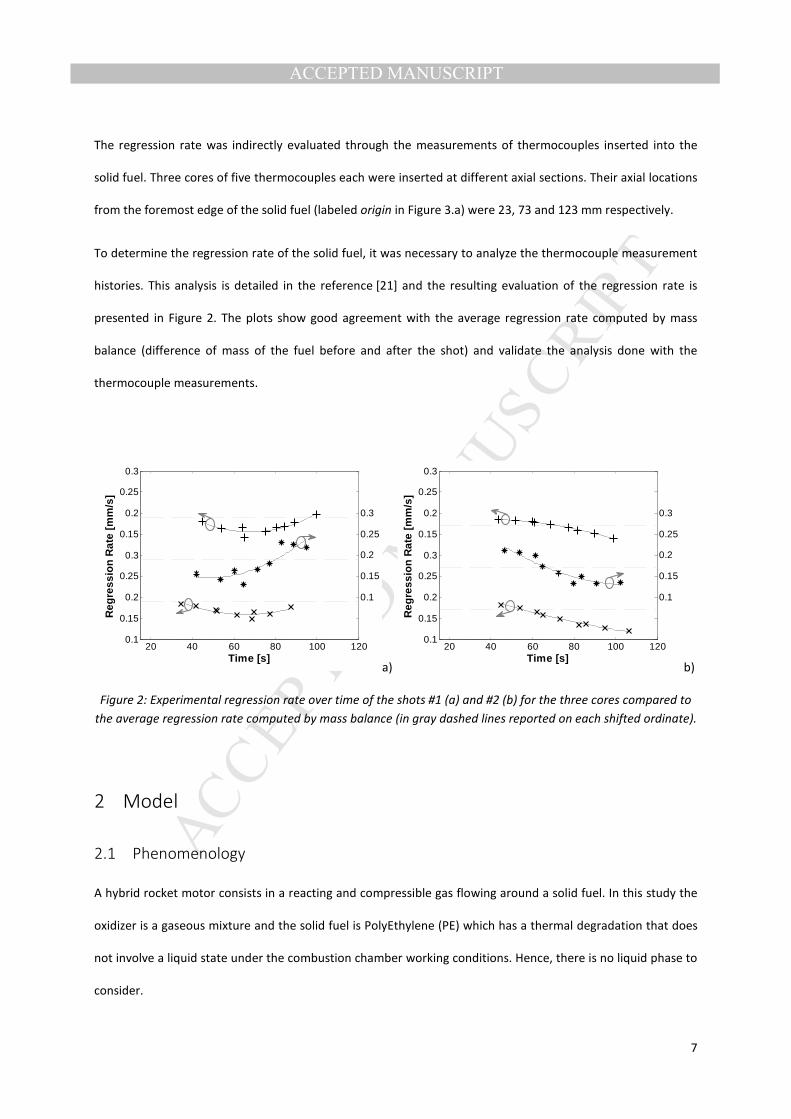
The regression rate was indirectly evaluated through the measurements of thermocouples inserted into the
solid fuel. Three cores of five thermocouples each were inserted at different axial sections. Their axial locations
from the foremost edge of the solid fuel (labeled origin in Figure 3.a) were 23, 73 and 123 mm respectively.
To determine the regression rate of the solid fuel, it was necessary to analyze the thermocouple measurement
histories. This analysis is detailed in the reference [21] and the resulting evaluation of the regression rate is
presented in Figure 2. The plots show good agreement with the average regression rate computed by mass
balance (difference of mass of the fuel before and after the shot) and validate the analysis done with the
thermocouple measurements.
a) b)
Figure 2: Experimental regression rate over time of the shots #1 (a) and #2 (b) for the three cores compared to
the average regression rate computed by mass balance (in gray dashed lines reported on each shifted ordinate).
2 Model
2.1 Phenomenology
A hybrid rocket motor consists in a reacting and compressible gas flowing around a solid fuel. In this study the
oxidizer is a gaseous mixture and the solid fuel is PolyEthylene (PE) which has a thermal degradation that does
not involve a liquid state under the combustion chamber working conditions. Hence, there is no liquid phase to
consider.
0.1
0.15
0.2
0.25
0.3
0.1
0.15
0.2
0.25
0.3
0.15
0.2
0.25
0.3
20 40 60 80 100 120
Reg
ress
ion
Rat
e [m
m/s
]
Time [s]
0.1
0.15
0.2
0.25
0.3
0.1
0.15
0.2
0.25
0.3
0.15
0.2
0.25
0.3
20 40 60 80 100 120
Reg
ress
ion
Rat
e [m
m/s
]
Time [s]

MANUSCRIP
T
ACCEPTED
ACCEPTED MANUSCRIPT
8
The numerical model considers the solid phase of the fuel and the gaseous phase of the compressible and
unsteady gas flow. The governing equations includes the Navier-Stokes equations and the species equations.
Since the interaction between turbulence and the chemistry is not well understood by the authors, it has been
chosen to not use any turbulence model. The transport equations are expressed in a vector form [13] (see Eq.
1).
"#"� + "%&"�� = "(&"�� + ) Eq. 1
Where, # = * ��+,-���., %& = * �+��+�+, + /�,0- + 1+��+���
., (& =2334
06�,+,6�, + � 7879:��� 7;<79: =>>? and ) = * 00@A + @B@�
. where and C refer to
space dimensions and ! refers to each specie considered into the chemical processes. The term ) accounts for
the source or sink phenomenon. While chemical reactions take place, the rate at which each specie is created
or consumed is expressed by @� (Eq. 2). Furthermore, the chemical reactions affect the energy balance
releasing energy (combustion) or absorbing it (pyrolysis). The thermal power induced by chemistry processes is
accounted by @A (Eq. 3). The last process which is taken into account in the source term is the one related to
radiative heat transfer (detailed below) lumped into the term @B.
@� = D� E0�′′�G − �′�G1 × �G0�1G Eq. 2
@A = E @� ∙ ℎ�0�1� Eq. 3
According to literature [13], [25], the radiative heat transfer plays an important role (10 to 60 % of the total
heat exchange with the solid fuel) in the working conditions of hybrid rocket engines. The chosen model is the

MANUSCRIP
T
ACCEPTED
ACCEPTED MANUSCRIPT
9
Discrete Ordinate Method (DOM) [26] because it spans a wide range of optical thicknesses. In this case the
solid fuel is optically thick compared to the gas phase. Usually the absorption and emissivity are considered
constant and uniform on each phase.
The absorption coefficient for the solid fuel phase was set at 10 mm-1
. The absorption was measured on an
optical test bench [27]. The gas phase is based on the literature [28]–[31] that indicates a wide range of
variation for the absorption coefficient in combustion applications, in particular as a function of soot
concentration. In this study, an intermediate value of 0.05 mm-1
was used. For emissivity, the coefficients used
were 0.2 and 0.5 for solid and gas phase respectively. Lastly, as the DOM uses angular discretization to solve
the Radiative Transfer Equation, 12 ordinate directions were used.
The pyrolysis of PE is led by random scission which produces a wide range of various species by breaking the
polymer chain into smaller and smaller fragments. Experimentally, pyrolysis byproducts were quantified by gas
chromatography and mass spectroscopy. The results [20] show that more than forty different species should be
taken into account. As a first approach, only ethylene C2H4 was included as a pyrolysis byproduct. Thus, the
reaction is HDPE gives C2H4. The rate of the reaction is described by an Arrhenius type law. The numerical
values used for describing the pyrolysis kinetic is discussed in §2.3 since two different models are compared in
the frame of a parametric study.
The combustion mechanism involves the overall reaction of ethylene with oxygen (Eq. 4) and the oxidation of
carbon monoxide in a bidirectional reaction (Eq. 5). The kinetic parameters of the combustion mechanism are
adapted from Westbrook and Dryer [24] and reported in Table 2 in the International System of units.
� = � × �K × -� L−��ℛ ∙ �M × N�OP × N�OQ R
[m, kmol, s]
S %T/V
[K-1
]
T W
XYZ[ + 2. ^Y → 2. X^ + 2. ZY^ Eq. 4 13.5×10⁹ 15100 0.1 1.65
X^ + 1 2a ^Y ↔ X^Y Eq. 5 → 02.239×10
12 20140 1 0.5
Eq. 5 ← 02.121×10¹⁷
-0.5 53800 1 N/A
Table 2: Kinetic parameters for the combustion model.

MANUSCRIP
T
ACCEPTED
ACCEPTED MANUSCRIPT
10
Finally, into the gas phase, gradient of temperature and chemical specie concentrations imply gradient of
physical properties of the fluid. These physical properties must be modeled by mixing rules as a function of the
local temperature and chemical specie concentrations. Table 3 lists models used in the gas phase and the value
used in solid phase. In the solid fuel, the physical properties have been considered constant.
Solid phase Gas phase
Density [kg.m-3
] 0940 ideal gas law
Viscosity [Pa.s] N/A mix kinetic theory Wilke method [22], [23]
Specific heat [J.kg-1
.K-1
] 2200 mix JANAF method
Thermal conductivity [W.m-1
.K-1
] 0000.38 mix kinetic theory Wilke method [22], [23]
Mass diffusivity [m2.s
-1] N/A multi component Wilke and Lee formulation [22]
Table 3: Physical properties of the solid and gas phases.
2.2 Geometrical model and meshing
The combustion chamber has a geometry of revolution, thus the model is used in a 2-D axisymmetric
framework. Figure 3.b details the boundary conditions. The inlet is characterized by the test conditions on
which the mass flow rate and the gaseous mixture of oxygen and nitrogen (synthesized in Table 1) depend on.
All the simulations were conducted at a fixed inlet temperature of 280 K. At the outlet, the pressure was fixed
at the atmospheric pressure of 1×10⁵ Pa. The symmetry axis is automatically managed by the solver. It keeps at
zero all fluxes (convection and diffusion) across this boundary. All the walls, including the interface, have a no-
slip condition (c = 0). The outer boundaries of the solid fuel domain were set to be adiabatic. At the interface
the energy equation is resolved considering that from the solid side the velocity terms are null (+ = 0). At the
interface takes place surface reactions modeling the thermal degradation of the solid fuel. The instantaneous
energy flux balance through the interface is expressed by Eq. 6.

MANUSCRIP
T
ACCEPTED
ACCEPTED MANUSCRIPT
11
� "�"�dePf + �ePf E � "��"� g∆Zi,� + j kl,���8m8n o + pfqBPr
= � "�"�distu + �istu�� g∆Zi + j k��8m8n o + pfv�f[
Eq. 6
a)
b)
Figure 3: Dimensions in millimeters (a) of the geometrical domain with boundary conditions outlined (b).
The quality of the meshing has an influence on both the convergence efficiency of the solver and the accuracy
of the results. Several meshing iterations were done and few of them were quantitatively compared to each
other (Table 4). Since combustion chamber pressure is one of the main parameter for experimental
comparison, the grid sensitivity analysis is focused on this particular parameter. It is found that combustion
chamber pressure is mainly dependent of the nozzle throat wall mesh size (see Figure 4). Nevertheless, the loss
of accuracy in pressure with the coarsest tested grid remains under 2 %.
Meshing #5 #11 #15 #16
Overall number of nodes (/1000) 22.6 35.3 25.9 25.4
Interface Inlet Outlet
Walls
Symmetry axis
origin

MANUSCRIP
T
ACCEPTED
ACCEPTED MANUSCRIPT
12
Nozzle wall mesh size [µm] 23 46 00.8 00.8
Solid fuel wall mesh size [µm] 50 09 10 10
Pressure discrepancy [%] +0.85 -1.99 +1.14 +1.42
Table 4: Grid sensitivity parameters.
Figure 4: Combustion chamber pressure dependency over the mesh size at the nozzle throat wall.
Thus, the grid iteration was mainly driven by less tangible factors such as convergence efficiency or overall grid
quality. The grid that is finally adopted for this study contains more than 25,000 cells (Figure 5.a) and all
patches are structured – only quad elements were used. As the walls have a no-slip condition, meshing near
the walls was refined to 10 µm. It allows a fairly good description of the momentum and thermal boundary
layers (typically around ten meshes as shown by Figure 5.b). In the combustion zone, the cross section of the
flame is discretized with meshes of at most 0.5 mm.
a)
3.4
3.45
3.5
3.55
3.6
0 10 20 30 40 50
Pre
ssu
re [
ba
r]
Mesh size [µm]
Pressure level of preignition of shot #2

MANUSCRIP
T
ACCEPTED
ACCEPTED MANUSCRIPT
13
b)
Figure 5: Geometrical domain meshing (a). Close-up of temperature mapping and the boundary layer near solid
fuel wall (b).
The interface between the solid fuel and the gas phase is where the pyrolysis reaction takes place. However, to
the best of authors' knowledge, CFD-ACE does not manage by itself the modification of the geometry while the
surface of the solid fuel is being consumed. However, it remains possible to take this into consideration by a
user subroutine written in Fortran. This addition was carried out in this study.
Previous numerical studies on hybrid rocket engines [4]–[7] demonstrated the feasibility of modifying the
meshing to track the solid/gas interface while the solid fuel is regressing. In these studies, the domain is located
close to the interface so that the geometry of the whole combustion chamber is not represented. Therefore,
the initial interface is straight, which simplifies the algorithm. Without being exhaustive, more complex – yet
very effective – methods exist for capturing a sharp and moving interface. The first that could have been used
is the volume of fluid method [32]–[34] usually applied to an immersed body and free surface. This method has
the advantage of using a fixed meshing grid. In that class of algorithm, local mesh refinement [35] could also
have been an option in this study. Although it is usually applied to catch flow discontinuities rather than the
solid/fluid interface. Reference [36] showed that this method is suitable for solid propellant combustion. Lastly,
the level set method has been used for solid propellant rocket numerical simulations [37] as well, showing that
singular geometries can be considered. Nevertheless, none of these methods were found practical for this
study case or applicable in CFD-ACE. The development of a dedicated algorithm using meshing deformation
was therefore preferred.
Solid fuel
≈ 1

MANUSCRIP
T
ACCEPTED
ACCEPTED MANUSCRIPT
14
Since the solid fuel is a convex shape, when the shape shrinks, there is a risk that some portions of the
boundary intersect others. In terms of meshing, this leads to negative volume cells which immediately crash
the calculation. In a previous study [4]–[7] the problem did not arise thanks to the flat geometry of the solid
fuel. To circumvent this drawback, the main idea was to make sure that the nodes which are moved at the
solid/gas interface never cross the direction of displacement of another node. To that end, the algorithm relies
on the initial meshing to ensure that when it is deformed by the regression, no intersection can occur. Along
the solid/gas interface, two adjacent faces are considered Fi and Fj (in Figure 6.a). They share one common
node Ni which is a candidate for displacement since it is on the interface. Each face is the boundary of two cells:
the first in the gas phase and the second in the solid phase. The cells Ci and Cj are the cells belonging to the
solid phase that are bounded by Fi and Fj respectively. These two cells have two nodes in common: Ni and Nj.
The node Ni being the candidate considered, Nj indicates its direction of displacement ��. By ensuring that the
node Ni moves along that direction only, �� remains constant during the whole computation. Hence, this
algorithm has to be run only once, at the first iteration of the solver.
In terms of meshing constraints, this algorithm implies that each node at the interface has a matching node on
either side of the interface. On Figure 6.a the solid phase is used, but the gas phase can also be used, the
direction of displacement �� just needs to be correctly oriented. To do that, the meshing has to be generated by
a sweep along the interface (Figure 6.b).
a) b)
Figure 6: Algorithm workflow for searching the direction of displacement (a). Swept meshing along the interface
and the angle between transverse direction of the meshing and the normal (b).
F
Fi
Ni
Nj
Cj
Ci
��
Gas

MANUSCRIP
T
ACCEPTED
ACCEPTED MANUSCRIPT
15
Usually, the local normal ��� of the surface is not parallel to the direction of displacement ��. Since regression is a
normal phenomenon, the formulation must consider the angle between the two vectors (Eq. 7). However,
when the angle between the normal and the direction is too high (typically more than 45°), experience showed
that a saw tooth profile arises after a certain amount of computation time. It was also observed that this
phenomenon tends to degenerate once it begins to happen. This behavior is attributed to the inner product
tending to zero when the angle is close to 90°. To mitigate the influence of the inner product at high angles, it is
limited by the expression of Eq. 8 where w was set to the numerical value of 3. The bias between the two
expressions is below 1 % for angles below 30°.
x� = ��0�1y��� ∙ ��y × �� Eq. 7
z{ = 1 + -� |−w × y��� ∙ ��y} − -� 0−w1w × y��� ∙ ��y Eq. 8
2.3 Workflow and parametric study
Prior to get a numerical state describing the working condition of the combustor, several steps must be
conducted.
Firstly, the pressure that builds up in the combustion chamber when a flow of gas goes through the nozzle is
dependent of the mass flow rate and the throat area. Both measurements from the experimental setup have
their respective margin of error. Consequently, when the experimental oxidizer mass flow rate is applied to the
numerical model that is meshed with the measured nozzle throat diameter, small discrepancies can be found.
In order to correct the numerical model, the pressure of the combustor prior the ignition is used to offset the
oxidizer mass flow rate in the numerical model until the resulting pressure match the one measured
experimentally (see Figure 1). This part of the workflow is labelled "initialization" in Figure 7.
Each iteration stats with initial conditions set with ambient pressure and temperature (1×10⁵ Pa and 280 K
respectively) and no flow field velocity. This part of the simulation is done without chemistry and radiative heat

MANUSCRIP
T
ACCEPTED
ACCEPTED MANUSCRIPT
16
transfer because the fluid stays relatively cold. The flow field is computed until it stabilizes to a pressure
corresponding to the compression due to the throat of the nozzle.
When satisfying conditions are found, the flow field is used as initial condition for the ignition. The ignition is
achieved by imposing high temperature (1000 K) on the fore edge of the solid fuel surface. This high
temperature forces the pyrolysis mechanism to generate hot and reactive specie (C2H4). Upon mixing with the
oxygen in the combustion chamber, the combustion occurs which generates more heat. The heat, locally
generated by the combustion near the fore edge of the fuel, is conveyed by the flow downstream activating the
pyrolysis of the rest of the fuel surface. Ultimately, enough reducer is produced by the pyrolysis to entertain
the combustion and enough heat is produced by the combustion to entertain the pyrolysis. At this point the
combustion is self-sustaining, the high temperature boundary condition, modeling the ignition process, is
removed.
The flow field is let to progress until significant results are obtained.
Figure 7: Total workflow of the conducted simulations.
Ks� = t9l
Stabilization of the flow field
Uniform +, x, and � Constant !� ~9
Ignition
Combustion self-sustained
Stop ignition
Significant results
no
yes
Initialization
Igniting

MANUSCRIP
T
ACCEPTED
ACCEPTED MANUSCRIPT
17
From the experimental studies two regression rate kinetics have been found. The first set was evaluated by
TGA [20] while the second set was evaluated by the analysis of measurements from the thermocouples
inserted on the solid fuel during the shots of the test bench [21]. These evaluations led to Eq. 9 and Eq. 10
respectively (expressed in m.s-1
) where �f stands for the fuel surface temperature.
�� = 25.91 ∙ 10� × -� L−16875�f M Eq. 9
�� = 0.438 ∙ 10�� × -� L−843�f M Eq. 10
The discrepancies in regression rate models are attributed to the difference of pyrolysis reacting temperatures.
TGA was conducted with temperatures ranging from 633 to 773 K, while the fuel surface temperatures during
test bench shots reach more than 1000 K. Figure 8 shows that the swap of model occurs at around 900 K. Both
models are consistent with the results of HDPE pyrolysis analysis conducted by Lengellé [38] who compared his
own results with another work from Blazowski [39].
Figure 8: Regression rate as a function of the reciprocal fuel temperature shows good agreement between
thermogravimetry measurements with a high temperature degradation rate from other studies. The
experimental shots show another kinetics.
0.9 1 1.1 1.2 1.3 1.4 1.5 1.6
10-4
10-3
10-2
10-1
100
Reciprocal Temperature [K-1] ×××× 103
Reg
ress
ion
rat
e [m
m.s
-1]
ATGATG lin.exp. shotsexp. lin.LengelleBlazowski

MANUSCRIP
T
ACCEPTED
ACCEPTED MANUSCRIPT
18
Using the first regression model leads to predictable simulations (prediction of motor working conditions
thanks to lab-scale TGA experiment) while the second regression model leads to reproducible simulations
compared to experimental results. From the standpoint of a hybrid engine development framework (which was
not the case, but the exercise still has its value) smaller experiment could be in favor to obtain a regression
model. TGA is a lab scale experiment, standardized and therefore relatively inexpensive to run. On the
contrary, a test bench is already a quasi rocket engine to design, manufacture and operate. The level of
expenditure is significantly higher than TGA. Therefore, it is economically logical to favor TGA experiment to
produce the regression model and run simulations with it. In this case both models were available, giving the
rare opportunity to compare their CFD results (see Table 5 for conditions) and the results are discussed latter in
this paper. Still, applying TGA model into a working engine simulation, implies that the pyrolysis kinetic does
not vary significantly while the pressure, nature of the surrounding gas and heat flux is changed significantly
from the conditions encountered during TGA.
Two types of simulations have been conducted. The first is a static solid/gas interface, meaning that the
displacement of the interface while the solid would regress is not followed by the deformation of the meshing.
The resolution is still unsteady because of the Kelvin-Helmholtz instabilities generated in the fore section of the
combustion chamber. However, since there is no modification in the combustion chamber geometry, the
average flow characteristics are rapidly attained, within the range of one or two seconds of simulated time. The
second type of simulation has a moving solid/gas interface. In this case, the regression of the solid fuel over
time is followed by the deformation of the meshing. The additional sub-model of the meshing deformation
does not lead to a significant increase in computational time. Nevertheless, given the combustion chamber
geometry and the regression rate intensity, significant results can only be achieved within the range of a dozen
seconds of simulated time.

MANUSCRIP
T
ACCEPTED
ACCEPTED MANUSCRIPT
19
Regression rate model Test
fire
Pressure
[bar]
Oxygen
content
ratio [%]
Oxidizer
mass flow
rate [g.s-1
]
TGA
(Eq. 9)
Test bench
(Eq. 10)
Interface
Fixed #1.1 #1.2 #1 25.0 50 50
Moving #2 X #2 11.5 30 50
Table 5: Parameters grid of the conducted simulations.
3 Results and discussion
3.1 Comparison of the regression kinetic with static interface
The following results come from static interface simulation. Therefore there is no geometrical variation over
time that could lead to the regression rate measurement. However, the pyrolysis models expressed by Eq. 9
and Eq. 10 give the regression rate as a function of the surface temperature. In this paragraph, regression rate
is thus computed from surface temperature.
In the case of the kinetic parameters from TGA (simulation #1.1 on Figure 9) the fuel surface temperature
matches the measurements on the test bench within a 5 % range. However, an average regression rate of
0.53 mm.s-1
is found while experimentally the value was 0.17 mm.s-1
(+212 % of error). This large discrepancy is
attributed to the kinetic parameters from TGA which are not suited for combustor working conditions. With a
solid fuel wet surface area of 22×103 mm
2 and a density of 940 kg.m
-3, the total mass flow rate is overestimated
by 13 %. With a shift of the thermodynamic properties of the gases passing through the nozzle, it explains why
the averaged pressure of 30 bar is also overestimated by 20 %.
Another aspect that must be considered for static interface simulations is the unsteadiness of the heat transfer
into the solid fuel. Without moving the interface with the diffusive heat wave, the fuel surface temperature
increases. This behavior is attributed to the fact that without the heat sink generated by the moving interface
the solid fuel temperature must rise to balance the incoming flux with the limited (the solid fuel does not
diffuse heat fast enough) subsurface flux. This bias caused by the geometrical steadiness of the interface is
overcome in the next simulation (simulation #1.2) by replacing the solid fuel with a boundary condition for the

MANUSCRIP
T
ACCEPTED
ACCEPTED MANUSCRIPT
20
energy equation. Since the solid fuel is consumed at the interface, the boundary condition is like a sink term
expressed by Eq. 11. It derives from Eq. 12 [38] which gives the amount of heat absorbed by the solid fuel for a
given surface temperature and therefore a given regression rate (� being the local normal of the surface).
�� = −� × ���� = �� ∙ �i ∙ ki × 0�f − ��1 Eq. 11
�0�1 − �� = 0�f − ��1 × -� L− � ∙ ����� M Eq. 12
In the case of the kinetic parameters from test bench measurements (simulation #1.2 on Figure 9), the fuel
surface temperature is overestimated by less than 3 % and the regression rate has a discrepancy within the
range of 0.03 mm.s-1
. With comparable regression rate, the average combustion chamber pressure of 25 bar is
in accordance with what was measured during the burn on the test bench. The pressure variations are also
comparable (see Figure 9.c). Since for this particular case, the solid fuel is removed and taken into account by a
boundary condition which does not account for the thermal inertia of the solid fuel, temperature variations at
the interface are found. These variations are represented by the error bars of Figure 9.a and can be as large as
300 K.

MANUSCRIP
T
ACCEPTED
ACCEPTED MANUSCRIPT
21
a) b)
c)
Figure 9: Comparisons on solid fuel temperature (a), regression rate (b) and pressure (c) of the experimental
data with the simulations results with a fixed interface.
3.2 Moving interface
This paragraph presents the results of the moving interface simulation. According to Table 5, this simulation is
conducted with the regression kinetic from the TGA results (Eq. 9) and applied to another test fire (#2, see
Figure 1.b) condition.
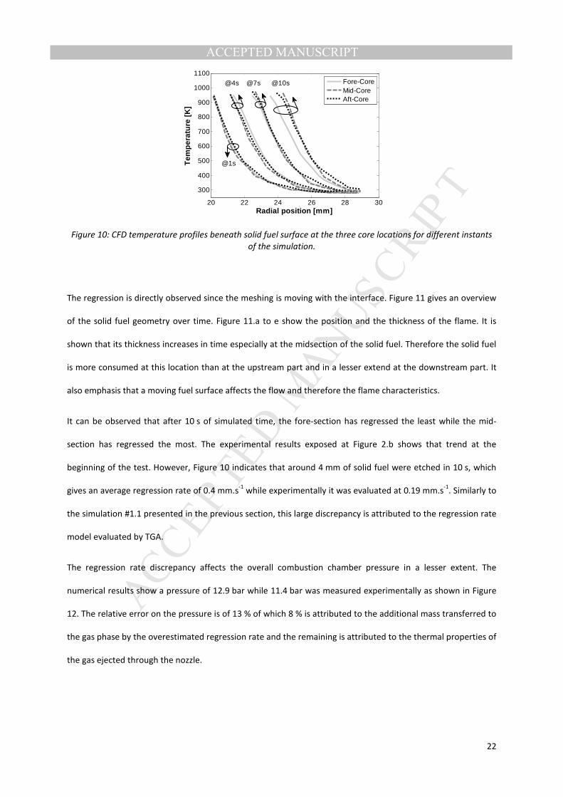
During this simulation the meshing follows the regression of the solid fuel. This allows the temperature field
under the solid fuel to reach a quasi-steady state. It is due to the interface moving at the same speed as the
thermal wave being diffused into the solid fuel. Thanks to the thermal inertia of the solid fuel, it is also noted
that the combustion instabilities does not impact the fuel subsurface temperatures. Subsurface temperature
profiles are plotted in Figure 10 and match the model of Eq. 12. The fuel surface temperature is about 950 K
which is comparable with the thermocouple measurements which vary from 800 to 1000 K (it is difficult to get
a precise measurement of the surface solid fuel temperature given the instrumentation [21]).
MANUSCRIP
T
ACCEPTED
ACCEPTED MANUSCRIPT
22
Figure 10: CFD temperature profiles beneath solid fuel surface at the three core locations for different instants
of the simulation.
The regression is directly observed since the meshing is moving with the interface. Figure 11 gives an overview
of the solid fuel geometry over time. Figure 11.a to e show the position and the thickness of the flame. It is
shown that its thickness increases in time especially at the midsection of the solid fuel. Therefore the solid fuel
is more consumed at this location than at the upstream part and in a lesser extend at the downstream part. It
also emphasis that a moving fuel surface affects the flow and therefore the flame characteristics.
It can be observed that after 10 s of simulated time, the fore-section has regressed the least while the mid-
section has regressed the most. The experimental results exposed at Figure 2.b shows that trend at the
beginning of the test. However, Figure 10 indicates that around 4 mm of solid fuel were etched in 10 s, which
gives an average regression rate of 0.4 mm.s-1
while experimentally it was evaluated at 0.19 mm.s-1
. Similarly to
the simulation #1.1 presented in the previous section, this large discrepancy is attributed to the regression rate
model evaluated by TGA.
The regression rate discrepancy affects the overall combustion chamber pressure in a lesser extent. The
numerical results show a pressure of 12.9 bar while 11.4 bar was measured experimentally as shown in Figure
12. The relative error on the pressure is of 13 % of which 8 % is attributed to the additional mass transferred to
the gas phase by the overestimated regression rate and the remaining is attributed to the thermal properties of
the gas ejected through the nozzle.
20 22 24 26 28 30
300
400
500
600
700
800
900
1000
1100
Radial position [mm]
Tem
per
atu
re [
K]
Fore-CoreMid-CoreAft-Core
@4s @7s @10s
@1s

MANUSCRIP
T
ACCEPTED
ACCEPTED MANUSCRIPT
23
a)
b)
c)
d)
e)
f)
Figure 11: Frames at 1 s (a), 3 s (b), 5 s (c), 7 s (d) and 9 s (e) showing the flame thickening overtime at the
midsection of the solid fuel where it regresses the fastest. The solid fuel interface is moving over time. The focus
on the fuel surface shows the evolution the fuel grain shape overtime (f).
Figure 12: Overestimation of the numerical pressure compared measurement conducted during the
experimental burn.
0 2 4 6 8 108
9
10
11
12
13
14
Time [s]
Pre
ssu
re [
bar
]
Num.Exp.
← iniPal surface posiPon
last computed surface position ↓
1s ← → 5s 9s ←

MANUSCRIP
T
ACCEPTED
ACCEPTED MANUSCRIPT
24
4 Conclusions and perspectives
The goal of this work was to build an operational model suited for hybrid rocket engine numerical simulations.
Some of the simplifications used were necessary to ease the development phase. Nevertheless, the model has
already produced interesting results (simulation #1.2). The fuel surface temperature is retrieved within 3% of
error. The regression rate is comparable to what was measured experimentally. The deviation is found less
than 0.03 mm.s-1
. With a comparable fuel mass flow rate, the combustion chamber pressure and its variations
are also reproduced.
The parameter study emphasized that regression kinetic deduced from TGA produce large inaccuracy (up to
+200%) on the regression rate despite fairly comparable fuel surface temperature. Consequently of this
overestimation, the averaged combustion chamber pressure is also affected.
From an hypothetical rocket development perspective one can understand why TGA kinetic could be
interesting. It is a much smaller and cheaper experimental setup than a combustor test bench. But this work
has clearly shown that results from TGA kinetic (simulation #1.1 and #2) are not comparable with the
experimental measurements. This shows that lab-scale experiments cannot be used to deduce a suitable
regression kinetic which is a fundamental input to the numerical model. Consequently, full scale combustor
test bench should precede numerical development, which is not a trivial workflow.
This work also demonstrates that it is possible to adapt the meshing to the unsteady geometry of the solid fuel
interface (simulation #2). With little computational effort, it can be done on a combustion chamber scale.
However, in order to produce significant results, the CFD solver must compute several seconds of simulation, if
not several tens of seconds. This later constraint may be found impractical. In that case, significant results are
obtained in shorter simulations by keeping the fuel interface fixed (simulation #1.1). As shown in this paper,
the solid fuel introduces a bias into the fuel surface temperature due the decreasing sub surface heat flux over
time. This side effect can be overcome by replacing the solid fuel by a boundary condition (simulation #1.2).
However it has been shown that the fuel grain geometry affects the flow pattern in the combustion chamber.
Since the regression rate is not uniform, it produces a fuel shape which can be computed with a moving
interface. The interaction between the flow pattern and the combustion chamber geometry gives valuable
information when compared to experimental data.
MANUSCRIP
T
ACCEPTED
ACCEPTED MANUSCRIPT
25
As for perspectives, the numerical model should be used to simulate the working conditions of other
experimental burns. It has been found in the literature that numerical works that does not take into account
turbulence are very rare. The lack of turbulence in this work is a major drawback. Therefore, turbulence model
should be added on the early stage of the follow ups. Finally, after two simulations showing large discrepancies
on regression rate using TGA kinetic, it should be definitively disregarded.
Acknowledgements
The present work was sponsored by CAPRYSSES project (ANR-11-LABX-006-01) funded by ANR through the PIA
(Programme d’Investissement d’Avenir) and is gratefully acknowledged. The earlier doctoral thesis work was
cofunded by Roxel and CNES, the French space agency.

MANUSCRIP
T
ACCEPTED
ACCEPTED MANUSCRIPT
26
References
[1] N. Serin and Y. A. Gogus, “A Fast Computer Code for Hybrid Motor Design, Eulec, and Results Obtained
for HTPB/O2 Combination,” in 39th AIAA/ASME/SAE/ASEE Joint Propulsion Conference & Exhibit, 2003.
[2] M. Stoia-Djeska and F. Mingireanu, “A Computational Fluid Dynamics Based Stability Analysis For
Hybrid Rocket Motor Combustion,” in 16th AIAA/CEAS Aeroacoustics Conference, 2010.
[3] J.-Y. Lestrade, J. Anthoine, and G. Lavergne, “Liquefying Fuel Regression Rate Modeling in Hybrid
Propulsion,” Aerosp. Sci. Technol., vol. 42, pp. 80–87, 2015.
[4] A. Antoniou and K. M. Akyuzlu, “A Physics Based Comprehensive Mathematical Model to Predict Motor
Performance in Hybrid Rocket Propulsion Systems,” in 41st AIAA/ASME/SAE/ASEE Joint Propulsion
Conference & Exhibit, 2005.
[5] K. Akyuzlu, R. Kagoo, and A. Antoniou, “A Physics Based Mathematical Model to Predict the Regression
Rate in an Ablating Hybrid Rocket Solid Fuel,” in 37th AIAA/ASME/SAE/ASEE Joint Propulsion
Conference & Exhibit, 2001.
[6] K. M. Akyuzlu, A. Antoniou, and M. W. Martin, “Determination of Regression Rate in an Ablating Hybrid
Rocket Solid Fuel Using a Physics Based Comprehensive Mathematical Model,” in 38th
AIAA/ASME/SAE/ASEE Joint Propulsion Conference & Exhibit, 2002.
[7] Y. Yang, C. Hu, T. Cai, and D. Sun, “Instantaneous Regression Rate Computation of Hybrid Rocket Motor
Based on Fluid-Solid Coupling Technique,” in 43rd AIAA/ASME/SAE/ASEE Joint Propulsion Conference &
Exhibit, 2007.
[8] J. L. Lin, “Two-Phase Flow Effect on Hybrid Rocket Combustion,” Acta Astronaut., vol. 65, no. 7–8, pp.
1042–1057, 2009.
[9] G. C. Cheng, R. C. Farmer, H. S. Jones, and J. S. Mcfarlane, “Numerical Simulation of the Internal
Ballistics of a Hybrid Rocket Motor,” in 32nd Aerospace Sciences Meeting & Exhibit, 1994.
[10] G. Gariani, F. Maggi, and L. Galfetti, “Simulation Code for Hybrid Rocket Combustion,” in 46th

MANUSCRIP
T
ACCEPTED
ACCEPTED MANUSCRIPT
27
AIAA/ASME/SAE/ASEE Joint Propulsion Conference & Exhibit, 2010.
[11] G. Gariani, F. Maggi, and L. Galfetti, “Numerical Simulation of HTPB Combustion in a 2D Hybrid Slab
Combustor,” Acta Astronaut., vol. 69, no. 5–6, pp. 289–296, 2011.
[12] G. Cai, P. Zeng, X. Li, H. Tian, and N. Yu, “Scale Effect of Fuel Regression Rate in Hybrid Rocket Motor,”
Aerosp. Sci. Technol., vol. 24, no. 1, pp. 141–146, 2013.
[13] V. Sankaran, “Computational Fluid Dynamics Modeling of Hybrid Rocket Flowfields,” in Fundamentals
of Hybrid Rocket Combustion and Propulsion, M. J. Chiaverini and K. K. Kuo, Eds. AIAA, 2007, pp. 323–
350.
[14] H. Tian, X. Sun, Y. Guo, and P. Wang, “Combustion Characteristics of Hybrid Rocket Motor with
Segmented Grain,” Aerosp. Sci. Technol., vol. 46, pp. 537–547, 2015.
[15] H. Tian, X. Li, P. Zeng, N. Yu, and G. Cai, “Numerical and Experimental Studies of the Hybrid Rocket
Motor with Multi-Port Fuel Grain,” Acta Astronaut., vol. 96, pp. 261–268, 2014.
[16] G. Cai and H. Tian, “Numerical Simulation of the Operation Process of a Hybrid Rocket Motor,” in 42nd
AIAA/ASME/SAE/ASEE Joint Propulsion Conference & Exhibit, 2006.
[17] Y.-S. Chen, T. H. Chou, B. R. Gu, J. S. Wu, B. Wu, Y. Y. Lian, and L. Yang, “Multiphysics Simulations of
Rocket Engine Combustion,” Comput. Fluids, vol. 45, no. 1, pp. 29–36, 2011.
[18] Y.-S. Chen, B. Wu, Y. Y. Lian, and L. Yang, “Multiphysics Computational Modeling of Hybrid Rocket
Combustion,” in 47th AIAA/ASME/SAE/ASEE Joint Propulsion Conference & Exhibit, 2011.
[19] Y. Chen, A. Lai, T. H. Chou, and J. S. Wu, “N2O-HTPB Hybrid Rocket Combustion Modeling with Mixing
Enhancement Designs,” in 49th AIAA/ASME/SAE/ASEE Joint Propulsion Conference, 2013.
[20] N. Gascoin, G. Fau, P. Gillard, and A. Mangeot, “Experimental Flash Pyrolysis of High Density
Polyethylene under Hybrid Propulsion Conditions,” J. Anal. Appl. Pyrolysis, vol. 101, pp. 45–52, 2013.
[21] N. Gascoin, A. Mangeot, P. Gillard, C. Marin, S. Rouvreau, J. Prevost, and D. Piton, “Firing Tests of
Hybrid Engine with Varying Oxidizer Nature and Operating Conditions,” J. Aerosp. Eng., vol. 228, no. 5,
pp. 755–765, 2014.

MANUSCRIP
T
ACCEPTED
ACCEPTED MANUSCRIPT
28
[22] B. E. Poling, J. M. Prausnitz, and J. P. O’Connell, The Properties of Gases and Liquids, 5th ed. McGraw-
Hill, 2007.
[23] R. B. Bird, W. E. Stewart, and E. N. Lightfoot, Transport Phenomena, 2nd ed. John Wiley & Sons Inc.,
2001.
[24] C. K. Westbrook and F. L. Dryer, “Simplified Reaction Mechanisms for the Oxidation of Hydrocarbon
Fuels in Flames,” Combust. Sci. Technol., vol. 27, no. 1–2, pp. 31–43, Dec. 1981.
[25] M. J. Chiaverini, “Review of Solid-Fuel Regression Rate Behavior in Classical and Nonclassical Hybrid
Rocket Motors,” in Fundamentals of Hybrid Rocket Combustion and Propulsion, M. J. Chiaverini and K.
K. Kuo, Eds. AIAA, 2007, pp. 37–125.
[26] W. A. Fiveland, “Three Dimensional Radiative Heat-Transfer Solutions by the Discrete Ordinates
Method,” J. Thermophys. Heat Transf., vol. 2, no. 4, pp. 209–316, 1988.
[27] A. Mangeot, “Étude Expérimentale et Développement Numérique d’une Modélisation des Phénomènes
Physicochimiques dans un Propulseur Hybride Spatial,” Université d’Orléans, 2012.
[28] P. B. Taylor and P. J. Foster, “The Total Emissivities of Luminous and non-Luminous Flames,” Int. J. Heat
Mass Transf., vol. 17, no. 12, pp. 1591–1605, 1974.
[29] R. Siegel, “Radiative Behavior of a Gas Layer Seeded with Soot,” Jul. 1976.
[30] R. O. Buckius and C.-L. Tien, “Infrared Flame Radiation,” Int. J. Heat Mass Transf., vol. 20, no. 2, pp. 93–
106, 1977.
[31] S. Prasanna, P. Rivière, and A. Soufiani, “Effect of Fractal Parameters on Absorption Properties of Soot
in the Infrared Region,” J. Quant. Spectrosc. Radiat. Transf., vol. 148, pp. 141–155, 2014.
[32] H. . Udaykumar, R. Mittal, and W. Shyy, “Computation of Solid–Liquid Phase Fronts in the Sharp
Interface Limit on Fixed Grids,” J. Comput. Phys., vol. 153, no. 2, pp. 535–574, 1999.
[33] C. Zhang, N. Lin, Y. Tang, and C. Zhao, “A sharp interface immersed boundary/VOF model coupled with
wave generating and absorbing options for wave-structure interaction,” Comput. Fluids, vol. 89, pp.
214–231, 2014.

MANUSCRIP
T
ACCEPTED
ACCEPTED MANUSCRIPT
29
[34] A. Gronskis and G. Artana, “A simple and efficient direct forcing immersed boundary method combined
with a high order compact scheme for simulating flows with moving rigid boundaries,” Comput. Fluids,
vol. 124, pp. 86–104, 2016.
[35] S. K. Sambasivan and H. S. UdayKumar, “Sharp interface simulations with Local Mesh Refinement for
multi-material dynamics in strongly shocked flows,” Comput. Fluids, vol. 39, no. 9, pp. 1456–1479,
2010.
[36] J. J. Choi, M. Cakmak, and S. Menon, “Simulations of Composite Solid Propellant Combustion Using
Adaptive Mesh Refinement,” in 49th AIAA Aerospace Sciences Meeting including the New Horizons
Forum and Aerospace Exposition, 2011.
[37] X. Wang, T. L. Jackson, and L. Massa, “Numerical simulation of heterogeneous propellant combustion
by a level set method,” Combust. Theory Model., vol. 8, pp. 227–254, 2004.
[38] G. Lengellé, “Solid-Fuel Pyrolysis Phenomena and Regression Rate, Part 1 : Mechanisms,” in
Fundamentals of Hybrid Rocket Combustion and Propulsion, M. J. Chiaverini and K. K. Kuo, Eds. AIAA,
2007, pp. 127–165.
[39] W.S. Blazowski, R.B. Cole, and R.F. Mc Alevy, “An Investigation of the Combustion Characteristics of
Some Polymers Using the Diffusion-Flame Technique,” Stevens Inst. of Technology, Technical Rept. TR
ME-RT 71004, June 1971.

MANUSCRIP
T
ACCEPTED
ACCEPTED MANUSCRIPT• Meshing can be adapted to follow the fuel geometry while fuel is regressing
• Combustion rates in both phases coupled through interface energy band mass balances
• The unsteadiness of the geometry influences the flow field and flame characteristics
• TGA kinetics are compared with those obtained in the combustion chamber