HAL Id: hal-00418197https://hal.archives-ouvertes.fr/hal-00418197

Submitted on 17 Sep 2009

HAL is a multi-disciplinary open accessarchive for the deposit and dissemination of sci-entific research documents, whether they are pub-lished or not. The documents may come fromteaching and research institutions in France orabroad, or from public or private research centers.

L’archive ouverte pluridisciplinaire HAL, estdestinée au dépôt et à la diffusion de documentsscientifiques de niveau recherche, publiés ou non,émanant des établissements d’enseignement et derecherche français ou étrangers, des laboratoirespublics ou privés.

Static et dynamic scheduling of maintenance activitiesunder the constraints of skills.

François Marmier, Christophe Varnier, Noureddine Zerhouni

To cite this version:François Marmier, Christophe Varnier, Noureddine Zerhouni. Static et dynamic scheduling of main-tenance activities under the constraints of skills.. Journal of Operations and Logistics, InternationalInstitute of Innovation, Industrial Engineering and Entrepreneurship I4e2, 2009, 2 (3), pp.I.1 - I.16.�hal-00418197�

Static and Dynamic Scheduling of Maintenance Activities Under the

Constraints of Skills

Francois Marmier, Christophe Varnier, Noureddine Zerhouni

FEMTO-ST Institut AS2M Dept. – CNRS/ENSMM/UFC/UTBM24, rue Alain Savary - 25000 Besancon - FRANCE

email: cvarnier@ens2m.fr

2009

Abstract

Skill management in industry is one of the most important factors required in order to ob-tain optimal performance of the production system. This is of particular importance in the fieldof maintenance where the different practical knowledge or skills are the working tools used. Weaddress, in this paper, both the assignment and scheduling problems that may be found in a main-tenance service. Each task that has to be performed is characterized by the level of skill required.The problem lies with making the decision of which time is the right time for the assignment andscheduling of the correct resource to do the task.

We introduce both static and dynamic scheduling, applied to the maintenance task assignment.To confer a maximum robustness to the obtained schedule, the approach proposed in this paper iscompleted by a proactive methodology which takes into account possible variations.

1 Introduction

To remain competitive, companies must decrease their costs as much as possible and optimize theirproduction means operations. In order to confer a better availability of equipment, and through it abetter availability of the company, the maintenance service intervenes. It deals with problems beforeand after breakdowns. This improvement mainly requires better management of the workforce and itsskills. The reactivity and the organization of the maintenance service will depend on the importanceof the treatment required.

Most information systems are built following the Herbert A. Simon [12] pyramid concept. Thelatter uses the classical diagram of organization: strategic / tactical / operational. Crespo-Marquezet al. proposed a decomposition to align maintenance management in this frame [1].

The highest level concerns non-schedulable tasks. This level concerns the maintenance servicepolicy and maintenance strategies definition. At the tactical level it is possible to schedule decisions.It concerns the implementation of maintenance policies for the assignment and scheduling of tasks andresources. This information is given to the operational level where the corresponding action is carriedout. Data concerning the work is recorded in the information system and available for decision-making.The figure, in figure 1, shows how maintenance services work.

If we focus on the tactical level of the maintenance service, we can observe that skills are importantto determine the role of the personnel and to take the appropriate decision. Grabot et al. carried outa study on nineteen companies to obtain their opinions on the operators’ assignment problem [4]. Itshowed that the management of operators, according to their skills, is important for industry leadersand that there is still no software available which takes this into account. 79% of the companies thinkthat the management of operators is useful or essential in scheduling. While in current software the

1

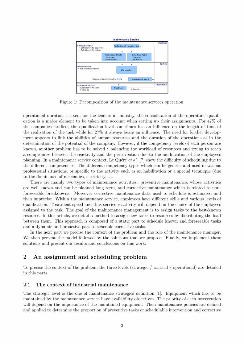
Figure 1: Decomposition of the maintenance services operation.

operational duration is fixed, for the leaders in industry, the consideration of the operators’ qualifi-cation is a major element to be taken into account when setting up their assignments. For 47% ofthe companies studied, the qualification level sometimes has an influence on the length of time ofthe realization of the task while for 27% it always bears an influence. The need for further develop-ment appears to link the abilities of human resources and the duration of the operations as in thedetermination of the potential of the company. However, if the competency levels of each person areknown, another problem has to be solved : balancing the workload of resources and trying to reacha compromise between the reactivity and the perturbation due to the modification of the employeesplanning. In a maintenance service context, Le Quere et al. [?] show the difficulty of scheduling due tothe different competencies. The different competency types which can be generic and used in variousprofessional situations, or specific to the activity such as an habilitation or a special technique (dueto the dominance of mechanics, electricity,...).

There are mainly two types of maintenance activities: preventive maintenance, whose activitiesare well known and can be planned long term, and corrective maintenance which is related to non-foreseeable breakdowns. Moreover corrective maintenance data used to schedule is estimated andthen imprecise. Within the maintenance service, employees have different skills and various levels ofqualification. Treatment speed and thus service reactivity will depend on the choice of the employeesassigned to the task. The goal of the maintenance management is to assign tasks to the best-knownresource. In this article, we detail a method to assign new tasks to resources by distributing the loadbetween them. This approach is composed of a static part to schedule known and foreseeable tasksand a dynamic and proactive part to schedule corrective tasks.

In the next part we precise the context of the problem and the role of the maintenance manager.We then present the model followed by the solutions that we propose. Finally, we implement thesesolutions and present our results and conclusions on this work.

2 An assignment and scheduling problem

To precise the context of the problem, the three levels (strategic / tactical / operational) are detailedin this parts.

2.1 The context of industrial maintenance

The strategic level is the one of maintenance strategies definition [1]. Equipment which has to bemaintained by the maintenance service have availability objectives. The priority of each interventionwill depend on the importance of the maintained equipment. Then maintenance policies are definedand applied to determine the proportion of preventive tasks or schedulable intervention and corrective

2

tasks which are non-schedulable. For this reason, failings in critical equipment are anticipated by apreventive policy.

At the tactical level the maintenance manager receives work requests. These requests come fromthe information system if tasks were planed like the preventive maintenance ones. They would alsocome from the production service if tasks were not scheduled such as the corrective maintenance ones.The maintenance policies are carried out by assigning and scheduling tasks to the different resources.After the assignment, work requests are re-injected as work orders in the information system.

Work orders are consulted by human resources at the operational level. Workers have to carryout tasks and to record indicators in the information system. These data permits us to know if thepolicies and the equipment priorities have to be modified.

2.2 Problems for the decision maker

Human resources are able to deal with the majority of maintenance tasks. Due to this versatility theyhave differences of efficiency following the type of tasks to achieve [4]. In this work, we suppose thatspare parts and tools are available for the intervention. The maintenance manager has an assignmentand scheduling problem of maintenance tasks [?]. He has to take into consideration the particularityof the maintenance context such as the differences between resources, the differences between tasks(some are preventive others are corrective) and the fact that some tasks are already assigned andscheduled and others are new ones. The manager has to schedule tasks to achieve some objectives likethe availability for equipment or the balancing of the load between the various resources.

The manager also has to take care of the different uncertainties of the context. Among uncertaintiesthere is the fact that some tasks are randomly generated by events like breakdowns but also the factthat most data used to make the schedule provide from estimations. Estimations provided fromdiagnosis. These ones, can be obtained with tools such as Case base Reasoning [?]. Therefore thedifferent level of competence of all operators are uncertain.

The issue is then an assignment and scheduling problem of maintenance tasks which is multi-objective and in an uncertain context.

2.3 A parallel machine problem

A maintenance service is an environment composed of m operators working in parallel. All of themare capable of performing each task, but not with the same efficiency. Moreover, the resource which isthe most effective for one task, may not necessarily be effective for all tasks. Since the main resourceare operators we are faced with a parallel machine problem, but with unrelated machines which isnoted R or Rm| β| γ , where β represents the processing characteristics and constraints and the γ fieldcontains the objective to be minimized [11].

Pfund and al. [10] presented a state of the art, unrelated parallel-machine. One part is moreprecisely devoted to the problem: Rm‖Cmax in the non-premptive task cases. Among all unrelatedparallel-machine scheduling problems, the ones which aim at minimizing the makespan, are the moststudied. Some authors have developed approximate methods, which can be executed quickly but haveno guarantee of reaching the optimum level. Ibarra and al. presented a methodology always used asa basis of comparison for current research in this field [6]. Their heuristic is based on a list algorithmand can lead to the worst case. Many others base their methodologies on a two-phase approach withan assignment problem solved by linear programming followed by a heuristic for the tasks which havenot been assigned during the first part. It is in the particular case of Hariri and Potts [5] or Lenstraand al. [7] who used amongst other things, the heuristic of Ibarra and al. in the second phase. Otherauthors have developed exact methods which make the obtaining of the optimal solution possible.Mokotoff and Chretienne [9] presented results obtained using an exact cutting plane algorithm andcompared it with the exact algorithms of Van de Velde [2] and Martello [8]. However the minimization

3

of the Cmax does not take into account priorities between tasks. In this way, problems which aim tominimize the weighted tardiness (Rm‖wjTj) are rarely found in literature.

In this paper we propose to decompose this problem in two sub-problems. The first one is a staticproblem, mainly to assign and to schedule preventive maintenance tasks. These tasks are considered asbeing well known. The second sub-problem deals with dynamic arrival of new tasks (mainly correctivemaintenance tasks). As most of the data is estimated, we consider in this sub-problem that theinformation about the tasks present some uncertainties. Task characteristics are modelled in the nextpart.

3 Model

Our problem is composed of two sub-problems. The first one consists in assigning and scheduling aset of m resources to a set of n known tasks. The second one consists in inserting a new task in acurrent schedule composed of m resources already assigned to n scheduled tasks. The m resources aresupposed to be available during the whole scheduling horizon.

3.1 Precise data

Given the fact that this problem is made with different precise and imprecise data, we model in thisfirst part the precise data.

3.1.1 Tasks

Task characterics are modelled as follows : for each task j,

• pj : standard duration of task j (this duration is subject to variations depending on the resourceassignment),

• rj : release date of task j,

• dj : due date of task j (this value is estimated in function of the current availability of theequipment concerned),

• wj : priority of the task due to the penalties which could be claimed if the treatment of task jis not performed on time.

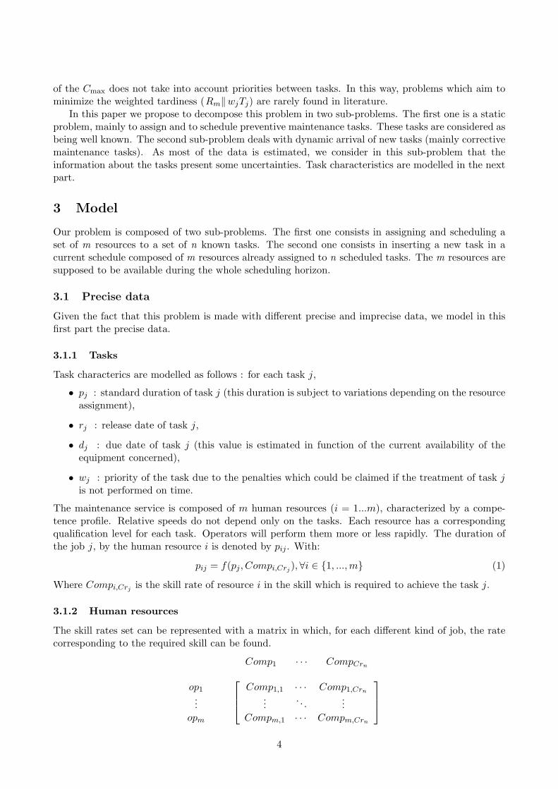
The maintenance service is composed of m human resources (i = 1...m), characterized by a compe-tence profile. Relative speeds do not depend only on the tasks. Each resource has a correspondingqualification level for each task. Operators will perform them more or less rapidly. The duration ofthe job j, by the human resource i is denoted by pij . With:

pij = f(pj , Compi,Crj ), ∀i ∈ {1, ...,m} (1)

Where Compi,Crj is the skill rate of resource i in the skill which is required to achieve the task j.

3.1.2 Human resources

The skill rates set can be represented with a matrix in which, for each different kind of job, the ratecorresponding to the required skill can be found.

Comp1 · · · CompCrn

op1...

opm

Comp1,1 · · · Comp1,Crn

.... . .

...Compm,1 · · · Compm,Crn

4

Skill levels are independent from one operation to another. A second factor being that, an operatorcan be the most efficient operator for one kind of operation and the least efficient for another.

3.2 Imprecise data

Imprecisions mainly concern corrective tasks which are non-foreseeable events. The diagnosis of theevent enable us to evaluate the duration of the task. The release date of the task depends mainly onthe date of the breakdown but also on the availability or on the delivery date of spare parts. The duedate of the task is determined regarding the objectives of the maintenance service.

For these reasons this different data is judged as being imprecise. Moreover, these tasks beinguncommon, the resource skill levels can vary. That is why, for the insertion of a new and correctivetask, task data is imprecise.

Concerning task duration, we assume that a part of the total treatment time is sensitive to vari-ations. The duration is then composed of an incompressible part and a variable part. Contrary toEsswein et al. who used a probability law in order to determine the presence of variations, we thinkthat a schedule is made up of task duration previsions [3]. The totality of the tasks is subject tovariations. The pij , rj or dj real values are obtained by using a normal law on their variable part.Each time we generate disturbances, we do it a hundred times and conserve the average.

3.3 Variables

The variables of our problem are the following ones for each task j:

• tj (j = 1...n) : starting of task j,

• xij (j = 1...n and i = 1...m) : 0-1 value representing the tasks’ assignment. xij = 1 if task j isassigned to a resource i, else xij = 0,

• Tj (j = 1...n) : lateness of task j,

• modj (j = 1...n) : represents the number of modifications made to the employees timetable.modj is incremented each time the assignment j is modified,

• PLi (i = 1...m) : potential load of the human resource i. It corresponds to the sum of thetasks durations assigned to i.

With :

PLi =n∑

j=1

xij ∗ pij (2)

3.4 Constraints

Constraints considered in this problem are as follows:

Each task has to be assigned only once to only one resource:

n∑j=1

xij = 1,∀i ∈ {1, ...,m} (3)

Task j cannot be planned before the equipment i is available:

tj > rj ,∀j ∈ {1, ..., n} (4)

5

Resources are disjunctive. That means that resource can only be used by a task at the sametime. Any couple of tasks (j1, j2) using the same resource is associated to the pair of disjunction(j1 ≺ j2) ∨ (j2 ≺ j1) [?]. Tasks using the same resource are then totally sequenced and there is adisjunction between the two inequalities of potential :

(tj1 − tj2 ≥ pj2) ∨ (tj2 − tj1 ≥ pj1) (5)

then :

∀t,∀i,n∑

j=1

aij(t) ≤ 1 (6)

3.5 Objective

Any equipment, which may be subject to maintenance activities, is framed with a contract. In thosecontracts, we find specifications regarding consequences of the availability losses for the maintenanceservice provider. These consequences are modelled with the weight wj . The penalties depend on theequipment contract, and they may be of a different form from one piece of equipment to another.

Tasks which are finished late, decreasing the equipment availability ratio, have an impact which isproportional to their weight. It implies that we have to minimize the total weighted tardiness.

minn∑

j=1

wjTj , (7)

With Tj the tardiness of the task j.

3.6 Optimization problem

Our problem can then be summarized as follow:

minn∑

j=1wjTj ,

So :n∑

j=1xij = 1, ∀i ∈ {1, ...,m},

tj > rj , ∀j ∈ {1, ..., n},

∀t,∀i,n∑

j=1aij(t) ≤ 1,

with Tj = max(O,Cj − dj) and Cj = tj + pij ,

with pij =n∑

j=1xij ∗ f(pj , compi,crj ).

4 Resolution approaches

The maintenance manager has to assign and schedule a set of known tasks to a set of resources. Thesetasks are mainly preventive ones which have t be scheduled in an horizon of medium term. This canbe done for each horizon period with a static scheduling approach. However regularly, in the short-term horizon, events (such as breakdowns) lead to the insertion of new tasks in the current schedule.Then, a new schedule must be generated with a dynamic scheduling approach. Both approaches arepresented in this part.

6

4.1 A static scheduling approach

In this part we detail the heuristic which has been developed in order to solve the static problem.This will be applied to the preventive maintenance task assignment. The developed heuristic is atwo-phase heuristic. The fact that tasks are assigned to human resources and the comparison of ourproblem with the problem of the parallel machines justifies that we balance and reduce the load. Thefirst phase consists in minimizing the makespan in order to balance the load between resources. Tominimize the makespan we introduce a lower bound. The second phase of the heuristic consists intaking into account due dates and release dates.

4.1.1 Lower Bound

We used the lower bound which is the simplest limit for a problem like Rm‖Cmax and that we find inparticular in the work of Ibarra and al. or of Mokotoff and Chretienne. It consists of taking for eachof the n tasks, the most powerful of the m resource and deducing the shortest duration pij for eachtask. Thus we obtain for the Lower Bound:

LB(Cmax) = max

{⌈1m

n∑i=1

pmini

⌉; maxi∈{1,...,m}

pmini

}(8)

with:pmin

j = min pij , j ∈ {1, ..., n} (9)

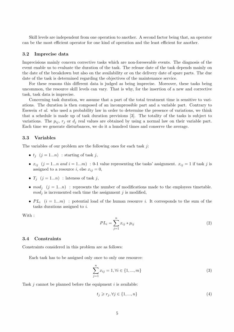
4.1.2 Assignment algorithm

This algorithm corresponds to the first heuristic phase and permits the makespan to be minimized.In a first stage, tasks are sorted according to the longest duration in a decreasing order and assigned,one by one, to the most efficient corresponding resource. If the assignment of a task to a resourceimplicates that the resource workload should be higher than the lower Bound, we try to assign thetask to the next most efficient resource which would have a lower workload than LB. This resourcemust not be the worst one for that type of task. In the letter case we will search the resource, whichwould finish the task treatment first. If this resource is the worst one, we would use the exceptionalgorithm. We propose two approaches in reply to these two problems.• The main algorithm :

L = { tasks order by decreasing longest duration pij } ;L = ∅;While (L 6= ∅) Then

k ← first task of L;i ← fastest resource for process task k;If

∑j∈L

pijxij + pik 6 LB Then

xik ← 1;xak ← 0, for a = 1 . . . n and a 6= i;L← L + k;L← L− k;

Else try to assign task k to the fastest resource l,With l = 1 . . . n and l 6= worst casethat respect

∑j∈L

pijxij + pik 6 LB;

If l not foundfind resource l so that:

7

minl=1...n

∑j∈L

pljxlj + plk

If l = worst caseException algorithm;

End IfEnd If

xlk ← 1;xak ← 0, for a = 1 . . . n and a 6= l;L← L + k;L← L− k;End If

End While

The exception algorithm evoked in the main algorithm has for objective to reduce as much aspossible the number of tasks assigned to the least efficient resource. The first task which would notbe treated by the worst resource is moved to the top of the list. If it is impossible to find one taskwhich would not be assigned to another one, it is assigned to the resource which would complete thetreatment of the first.• The exception algorithm :

Insert the first task on the list which would not be treatedby the worst resource at the top of the listIf all tasks ∈ L check pmax

j = max pij ThenThen assign the tasks without being worried by the factthat it could be to the worst resource

End

4.1.3 Tardiness penalties

Tardiness is the respect of the tasks due-dates. There exist various methods for taking tardiness intoaccount. In the previous algorithm we worked on minimizing the maximal completion time (Cmax).We compared results already obtained, reorganized with an Earliest Due Date (EDD) post-treatmentwithin each resource solution, with two other possibilities.

To consider tardiness, we replaced the pre-treatment with fixed tasks by decreasing longest dura-tion, by another with sorted tasks by the due-date dj in increasing order (EDD). In order to take intoaccount the potential penalties of each late task, we also tried a Weighted Shortest Processing Timefirst (WSPT) pre-treatment which sort tasks by their decreasing wi/pi.

After the assignment phase, the sorting of the tasks can generate a high number of late tasks. Toavoid this effect, we placed an EDD post-treatment sort for each resource assignment. Results of thisadaptation are presented in table 2, where H-EDD is our heuristic followed by an EDD post-treatment,EDD-H-EDD means that the Longest Processing Time (LPT) pre-treatment has replaced an EDDand finally WSPT-H-EDD means that the pre-treatment is a WSPT one.

5 A dynamic scheduling approach

As new tasks are mainly maintenance corrective tasks, their characteristics are stochastic as longas a diagnosis has not been made. When a new task has to be inserted and when their is not anyobvious solution, two ways are possible. The first way consists in generating a completely new staticscheduling. This methodology does not take into account any potential disturbance for employees who

8

have a new planning. The second one consists in searching new scheduling with a few modificationsto the current schedule. This kind of approach enables to disturbed as little as possible the existingplanning and the employees’ organization.

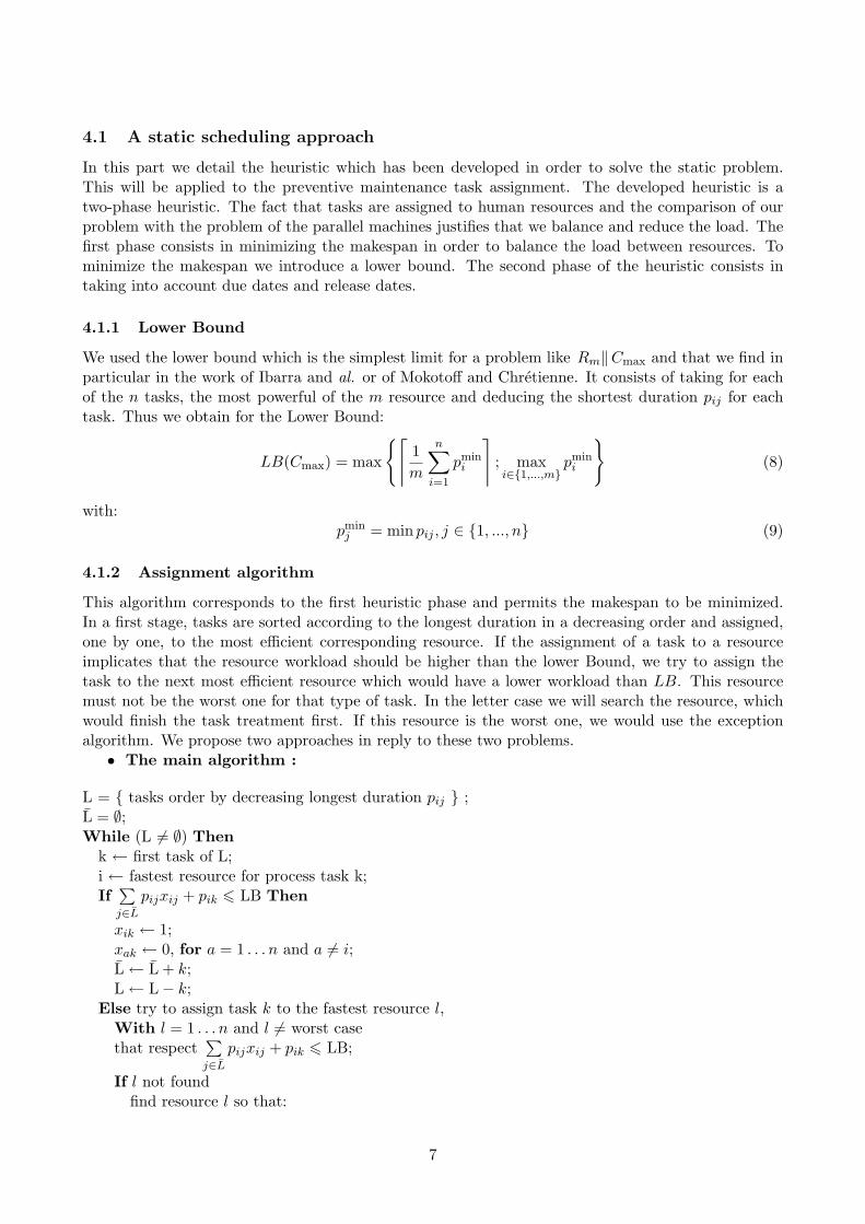
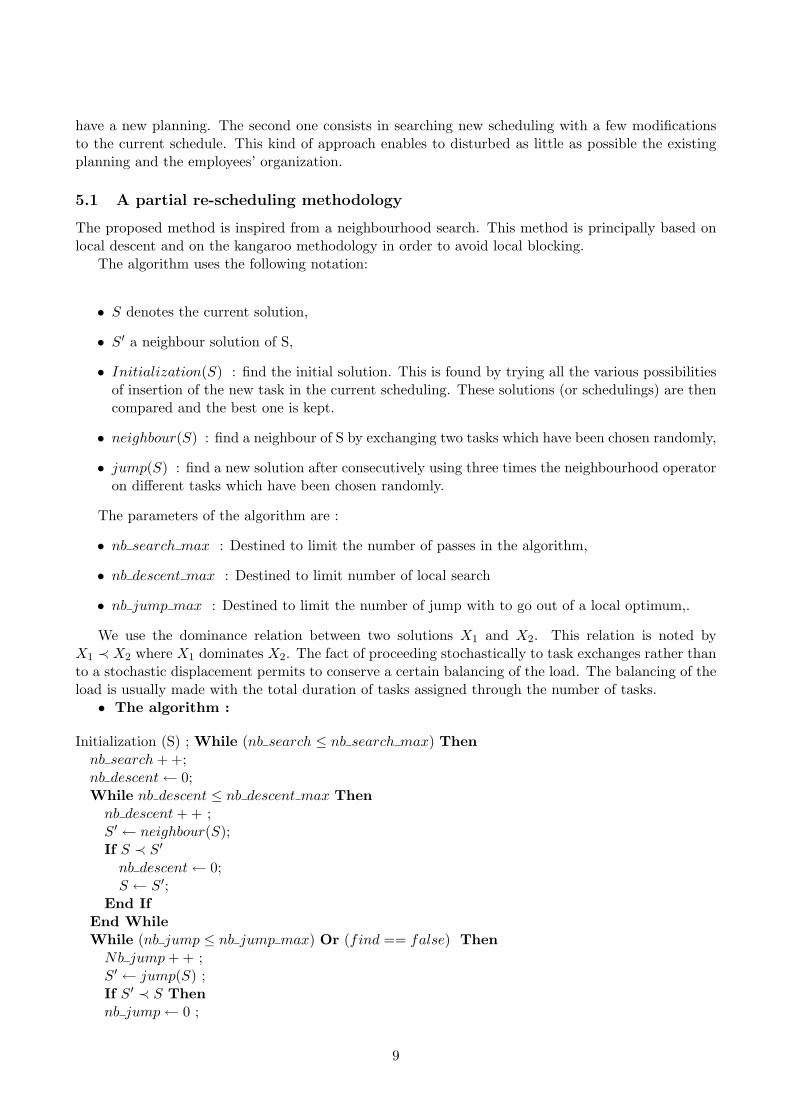
5.1 A partial re-scheduling methodology

The proposed method is inspired from a neighbourhood search. This method is principally based onlocal descent and on the kangaroo methodology in order to avoid local blocking.

The algorithm uses the following notation:

• S denotes the current solution,

• S′ a neighbour solution of S,

• Initialization(S) : find the initial solution. This is found by trying all the various possibilitiesof insertion of the new task in the current scheduling. These solutions (or schedulings) are thencompared and the best one is kept.

• neighbour(S) : find a neighbour of S by exchanging two tasks which have been chosen randomly,

• jump(S) : find a new solution after consecutively using three times the neighbourhood operatoron different tasks which have been chosen randomly.

The parameters of the algorithm are :

• nb search max : Destined to limit the number of passes in the algorithm,

• nb descent max : Destined to limit number of local search

• nb jump max : Destined to limit the number of jump with to go out of a local optimum,.

We use the dominance relation between two solutions X1 and X2. This relation is noted byX1 ≺ X2 where X1 dominates X2. The fact of proceeding stochastically to task exchanges rather thanto a stochastic displacement permits to conserve a certain balancing of the load. The balancing of theload is usually made with the total duration of tasks assigned through the number of tasks.• The algorithm :

Initialization (S) ; While (nb search ≤ nb search max) Thennb search+ +;nb descent← 0;While nb descent ≤ nb descent max Thennb descent+ + ;S′ ← neighbour(S);If S ≺ S′nb descent← 0;S ← S′;

End IfEnd WhileWhile (nb jump ≤ nb jump max) Or (find == false) ThenNb jump+ + ;S′ ← jump(S) ;If S′ ≺ S Thennb jump← 0 ;

9

S ← S′;find← true;End If

End WhileEnd While

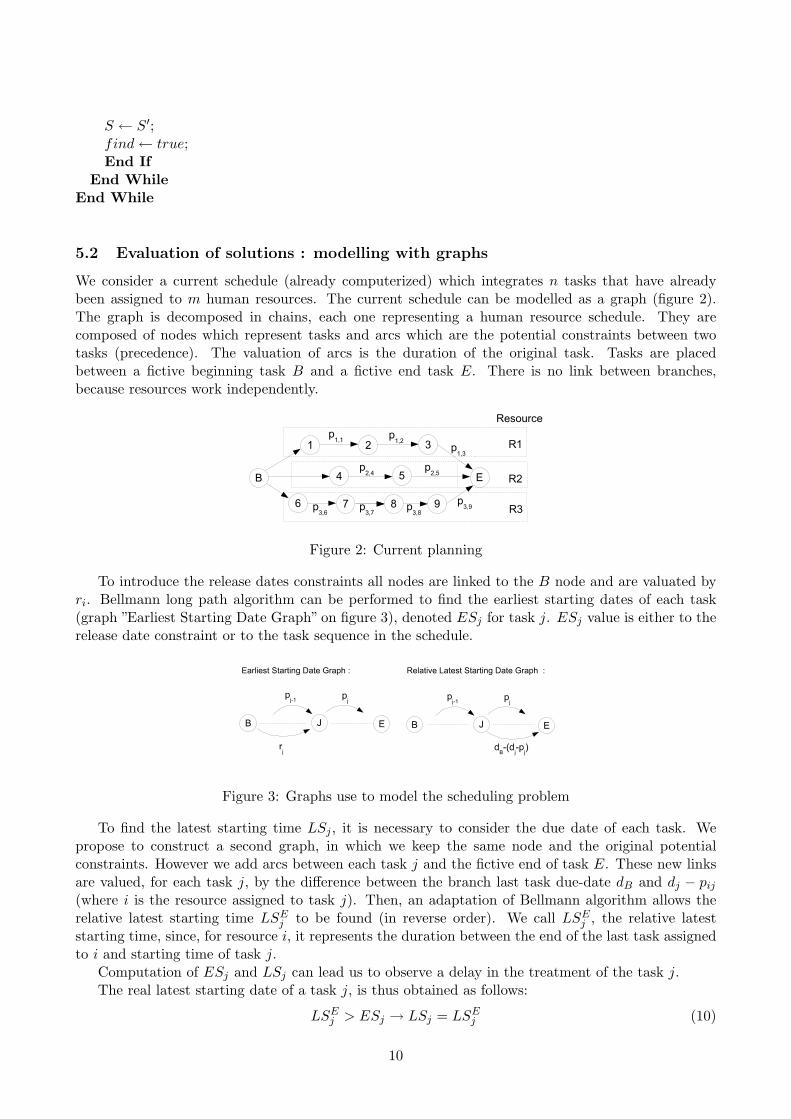
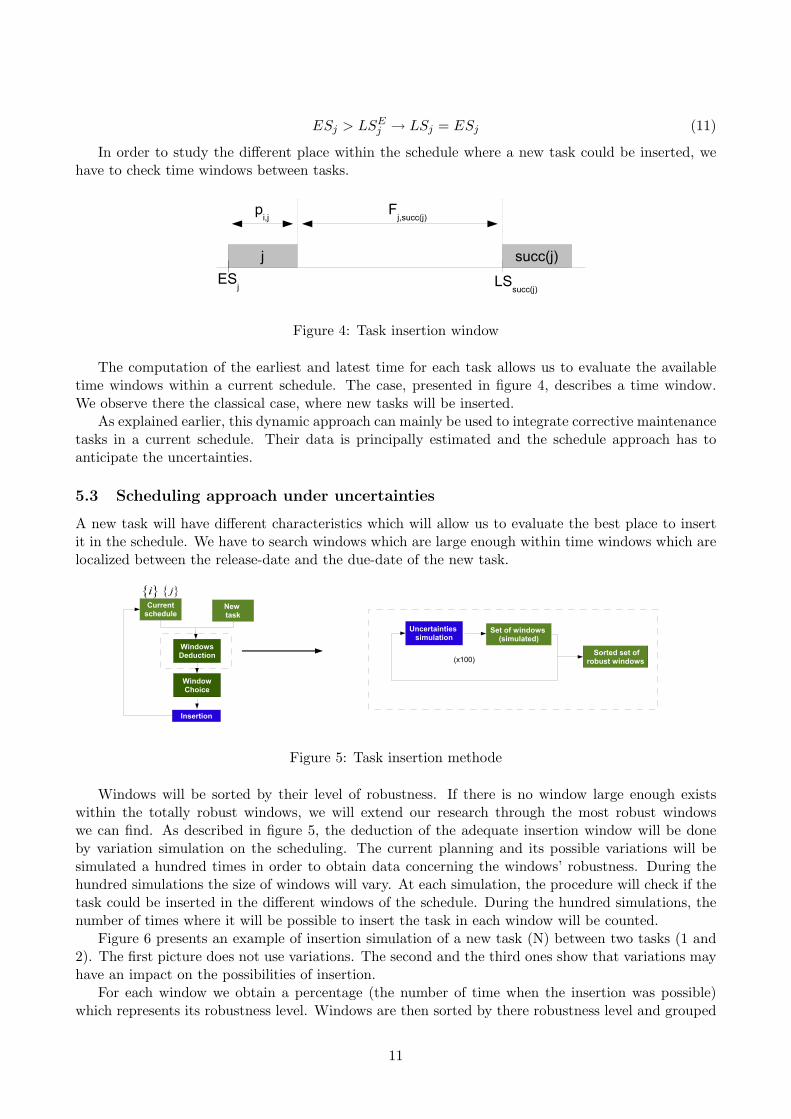
5.2 Evaluation of solutions : modelling with graphs

We consider a current schedule (already computerized) which integrates n tasks that have alreadybeen assigned to m human resources. The current schedule can be modelled as a graph (figure 2).The graph is decomposed in chains, each one representing a human resource schedule. They arecomposed of nodes which represent tasks and arcs which are the potential constraints between twotasks (precedence). The valuation of arcs is the duration of the original task. Tasks are placedbetween a fictive beginning task B and a fictive end task E. There is no link between branches,because resources work independently.

Figure 2: Current planning

To introduce the release dates constraints all nodes are linked to the B node and are valuated byri. Bellmann long path algorithm can be performed to find the earliest starting dates of each task(graph ”Earliest Starting Date Graph” on figure 3), denoted ESj for task j. ESj value is either to therelease date constraint or to the task sequence in the schedule.

Figure 3: Graphs use to model the scheduling problem

To find the latest starting time LSj , it is necessary to consider the due date of each task. Wepropose to construct a second graph, in which we keep the same node and the original potentialconstraints. However we add arcs between each task j and the fictive end of task E. These new linksare valued, for each task j, by the difference between the branch last task due-date dB and dj − pij

(where i is the resource assigned to task j). Then, an adaptation of Bellmann algorithm allows therelative latest starting time LSE

j to be found (in reverse order). We call LSEj , the relative latest

starting time, since, for resource i, it represents the duration between the end of the last task assignedto i and starting time of task j.

Computation of ESj and LSj can lead us to observe a delay in the treatment of the task j.The real latest starting date of a task j, is thus obtained as follows:

LSEj > ESj → LSj = LSE

j (10)

10

ESj > LSEj → LSj = ESj (11)

In order to study the different place within the schedule where a new task could be inserted, wehave to check time windows between tasks.

Figure 4: Task insertion window

The computation of the earliest and latest time for each task allows us to evaluate the availabletime windows within a current schedule. The case, presented in figure 4, describes a time window.We observe there the classical case, where new tasks will be inserted.

As explained earlier, this dynamic approach can mainly be used to integrate corrective maintenancetasks in a current schedule. Their data is principally estimated and the schedule approach has toanticipate the uncertainties.

5.3 Scheduling approach under uncertainties

A new task will have different characteristics which will allow us to evaluate the best place to insertit in the schedule. We have to search windows which are large enough within time windows which arelocalized between the release-date and the due-date of the new task.

Figure 5: Task insertion methode

Windows will be sorted by their level of robustness. If there is no window large enough existswithin the totally robust windows, we will extend our research through the most robust windowswe can find. As described in figure 5, the deduction of the adequate insertion window will be doneby variation simulation on the scheduling. The current planning and its possible variations will besimulated a hundred times in order to obtain data concerning the windows’ robustness. During thehundred simulations the size of windows will vary. At each simulation, the procedure will check if thetask could be inserted in the different windows of the schedule. During the hundred simulations, thenumber of times where it will be possible to insert the task in each window will be counted.

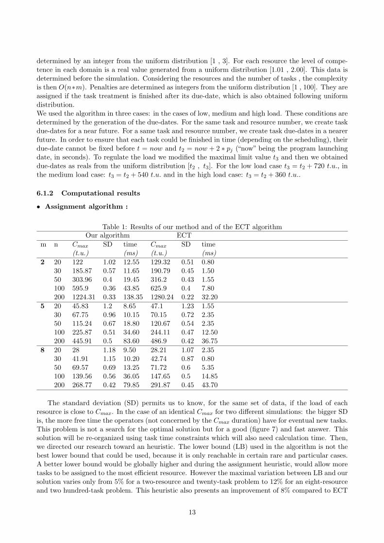
Figure 6 presents an example of insertion simulation of a new task (N) between two tasks (1 and2). The first picture does not use variations. The second and the third ones show that variations mayhave an impact on the possibilities of insertion.

For each window we obtain a percentage (the number of time when the insertion was possible)which represents its robustness level. Windows are then sorted by there robustness level and grouped

11

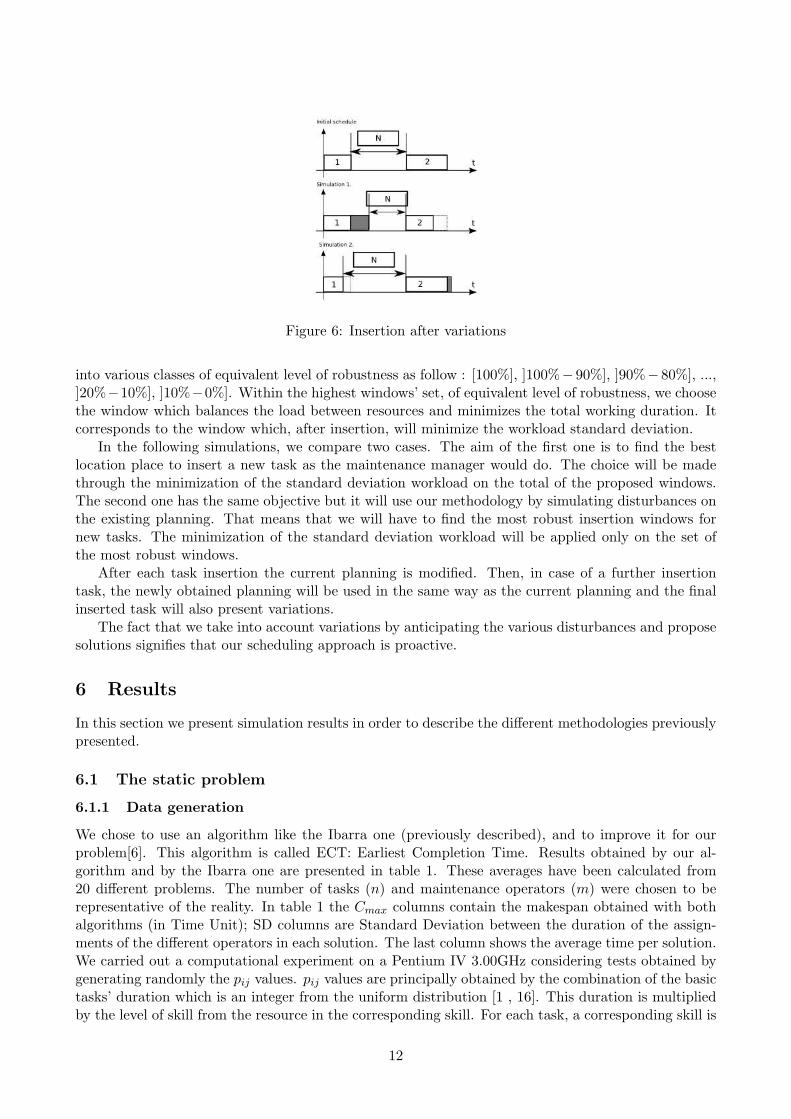
Figure 6: Insertion after variations

into various classes of equivalent level of robustness as follow : [100%], ]100%− 90%], ]90%− 80%], ...,]20%−10%], ]10%−0%]. Within the highest windows’ set, of equivalent level of robustness, we choosethe window which balances the load between resources and minimizes the total working duration. Itcorresponds to the window which, after insertion, will minimize the workload standard deviation.

In the following simulations, we compare two cases. The aim of the first one is to find the bestlocation place to insert a new task as the maintenance manager would do. The choice will be madethrough the minimization of the standard deviation workload on the total of the proposed windows.The second one has the same objective but it will use our methodology by simulating disturbances onthe existing planning. That means that we will have to find the most robust insertion windows fornew tasks. The minimization of the standard deviation workload will be applied only on the set ofthe most robust windows.

After each task insertion the current planning is modified. Then, in case of a further insertiontask, the newly obtained planning will be used in the same way as the current planning and the finalinserted task will also present variations.

The fact that we take into account variations by anticipating the various disturbances and proposesolutions signifies that our scheduling approach is proactive.

6 Results

In this section we present simulation results in order to describe the different methodologies previouslypresented.

6.1 The static problem

6.1.1 Data generation

We chose to use an algorithm like the Ibarra one (previously described), and to improve it for ourproblem[6]. This algorithm is called ECT: Earliest Completion Time. Results obtained by our al-gorithm and by the Ibarra one are presented in table 1. These averages have been calculated from20 different problems. The number of tasks (n) and maintenance operators (m) were chosen to berepresentative of the reality. In table 1 the Cmax columns contain the makespan obtained with bothalgorithms (in Time Unit); SD columns are Standard Deviation between the duration of the assign-ments of the different operators in each solution. The last column shows the average time per solution.We carried out a computational experiment on a Pentium IV 3.00GHz considering tests obtained bygenerating randomly the pij values. pij values are principally obtained by the combination of the basictasks’ duration which is an integer from the uniform distribution [1 , 16]. This duration is multipliedby the level of skill from the resource in the corresponding skill. For each task, a corresponding skill is

12

determined by an integer from the uniform distribution [1 , 3]. For each resource the level of compe-tence in each domain is a real value generated from a uniform distribution [1.01 , 2.00]. This data isdetermined before the simulation. Considering the resources and the number of tasks , the complexityis then O(n∗m). Penalties are determined as integers from the uniform distribution [1 , 100]. They areassigned if the task treatment is finished after its due-date, which is also obtained following uniformdistribution.We used the algorithm in three cases: in the cases of low, medium and high load. These conditions aredetermined by the generation of the due-dates. For the same task and resource number, we create taskdue-dates for a near future. For a same task and resource number, we create task due-dates in a nearerfuture. In order to ensure that each task could be finished in time (depending on the scheduling), theirdue-date cannot be fixed before t = now and t2 = now + 2 ∗ pj (“now” being the program launchingdate, in seconds). To regulate the load we modified the maximal limit value t3 and then we obtaineddue-dates as reals from the uniform distribution [t2 , t3]. For the low load case t3 = t2 + 720 t.u., inthe medium load case: t3 = t2 + 540 t.u. and in the high load case: t3 = t2 + 360 t.u..

6.1.2 Computational results

• Assignment algorithm :

Table 1: Results of our method and of the ECT algorithmOur algorithm ECT

m n Cmax SD time Cmax SD time(t.u.) (ms) (t.u.) (ms)

2 20 122 1.02 12.55 129.32 0.51 0.8030 185.87 0.57 11.65 190.79 0.45 1.5050 303.96 0.4 19.45 316.2 0.43 1.55100 595.9 0.36 43.85 625.9 0.4 7.80200 1224.31 0.33 138.35 1280.24 0.22 32.20

5 20 45.83 1.2 8.65 47.1 1.23 1.5530 67.75 0.96 10.15 70.15 0.72 2.3550 115.24 0.67 18.80 120.67 0.54 2.35100 225.87 0.51 34.60 244.11 0.47 12.50200 445.91 0.5 83.60 486.9 0.42 36.75

8 20 28 1.18 9.50 28.21 1.07 2.3530 41.91 1.15 10.20 42.74 0.87 0.8050 69.57 0.69 13.25 71.72 0.6 5.35100 139.56 0.56 36.05 147.65 0.5 14.85200 268.77 0.42 79.85 291.87 0.45 43.70

The standard deviation (SD) permits us to know, for the same set of data, if the load of eachresource is close to Cmax. In the case of an identical Cmax for two different simulations: the bigger SDis, the more free time the operators (not concerned by the Cmax duration) have for eventual new tasks.This problem is not a search for the optimal solution but for a good (figure 7) and fast answer. Thissolution will be re-organized using task time constraints which will also need calculation time. Then,we directed our research toward an heuristic. The lower bound (LB) used in the algorithm is not thebest lower bound that could be used, because it is only reachable in certain rare and particular cases.A better lower bound would be globally higher and during the assignment heuristic, would allow moretasks to be assigned to the most efficient resource. However the maximal variation between LB and oursolution varies only from 5% for a two-resource and twenty-task problem to 12% for an eight-resourceand two hundred-task problem. This heuristic also presents an improvement of 8% compared to ECT

13

for the eight-resource and two hundred-task problem, which is a large-sized problem. This is logicalbecause of the added treatment of this algorithm. That treatment time is slightly increased with ouralgorithm, but this is not perceptible for the program user, as it does not represent a problem.• Tardiness management :

Table 2: Tardiness considerationLow load Medium Load High Load

H-EDD∑Ui 3 22 148∑wiTi 173 1141 7301

Cmax 448 464 461EDD-H-EDD

∑Ui 33 71 136∑wiTi 1656 3487 6841

Cmax 456 473 468WSPT-H-EDD

∑Ui 3 21 143∑wiTi 162 1027 7142

Cmax 454 469 466

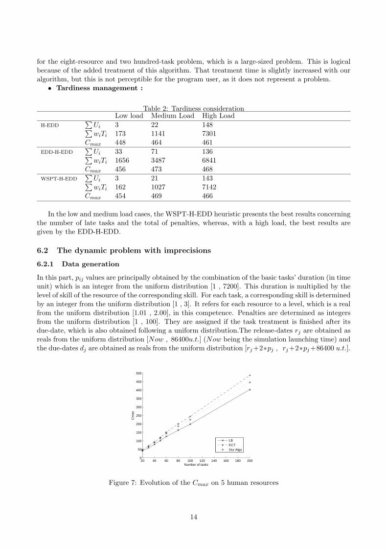
In the low and medium load cases, the WSPT-H-EDD heuristic presents the best results concerningthe number of late tasks and the total of penalties, whereas, with a high load, the best results aregiven by the EDD-H-EDD.

6.2 The dynamic problem with imprecisions

6.2.1 Data generation

In this part, pij values are principally obtained by the combination of the basic tasks’ duration (in timeunit) which is an integer from the uniform distribution [1 , 7200]. This duration is multiplied by thelevel of skill of the resource of the corresponding skill. For each task, a corresponding skill is determinedby an integer from the uniform distribution [1 , 3]. It refers for each resource to a level, which is a realfrom the uniform distribution [1.01 , 2.00], in this competence. Penalties are determined as integersfrom the uniform distribution [1 , 100]. They are assigned if the task treatment is finished after itsdue-date, which is also obtained following a uniform distribution.The release-dates rj are obtained asreals from the uniform distribution [Now , 86400u.t.] (Now being the simulation launching time) andthe due-dates dj are obtained as reals from the uniform distribution [rj +2∗pj , rj +2∗pj +86400 u.t.].

20 40 60 80 100 120 140 160 180 2000

50

100

150

200

250

300

350

400

450

500

Number of tasks

Cm

ax

LBECTOur Algo

Figure 7: Evolution of the Cmax on 5 human resources

14

6.2.2 Computational results

A classical schedule, which does not take into account the possible disturbance, will search the dif-ferent windows and will obtain a certain number of positions. Our procedure considers the differentdisturbances as explained above which is why we will compare insertion propositions on the sameproblem instances with and without uncertainties.

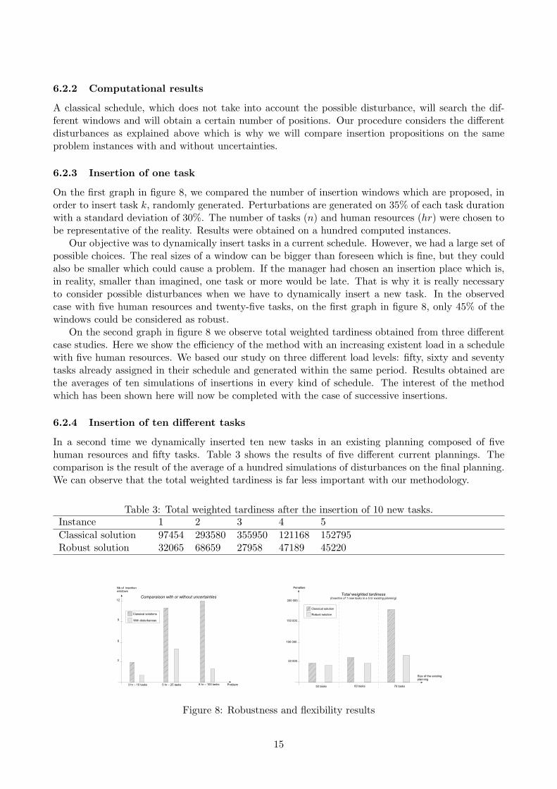
6.2.3 Insertion of one task

On the first graph in figure 8, we compared the number of insertion windows which are proposed, inorder to insert task k, randomly generated. Perturbations are generated on 35% of each task durationwith a standard deviation of 30%. The number of tasks (n) and human resources (hr) were chosen tobe representative of the reality. Results were obtained on a hundred computed instances.

Our objective was to dynamically insert tasks in a current schedule. However, we had a large set ofpossible choices. The real sizes of a window can be bigger than foreseen which is fine, but they couldalso be smaller which could cause a problem. If the manager had chosen an insertion place which is,in reality, smaller than imagined, one task or more would be late. That is why it is really necessaryto consider possible disturbances when we have to dynamically insert a new task. In the observedcase with five human resources and twenty-five tasks, on the first graph in figure 8, only 45% of thewindows could be considered as robust.

On the second graph in figure 8 we observe total weighted tardiness obtained from three differentcase studies. Here we show the efficiency of the method with an increasing existent load in a schedulewith five human resources. We based our study on three different load levels: fifty, sixty and seventytasks already assigned in their schedule and generated within the same period. Results obtained arethe averages of ten simulations of insertions in every kind of schedule. The interest of the methodwhich has been shown here will now be completed with the case of successive insertions.

6.2.4 Insertion of ten different tasks

In a second time we dynamically inserted ten new tasks in an existing planning composed of fivehuman resources and fifty tasks. Table 3 shows the results of five different current plannings. Thecomparison is the result of the average of a hundred simulations of disturbances on the final planning.We can observe that the total weighted tardiness is far less important with our methodology.

Table 3: Total weighted tardiness after the insertion of 10 new tasks.Instance 1 2 3 4 5Classical solution 97454 293580 355950 121168 152795Robust solution 32065 68659 27958 47189 45220

Figure 8: Robustness and flexibility results

15

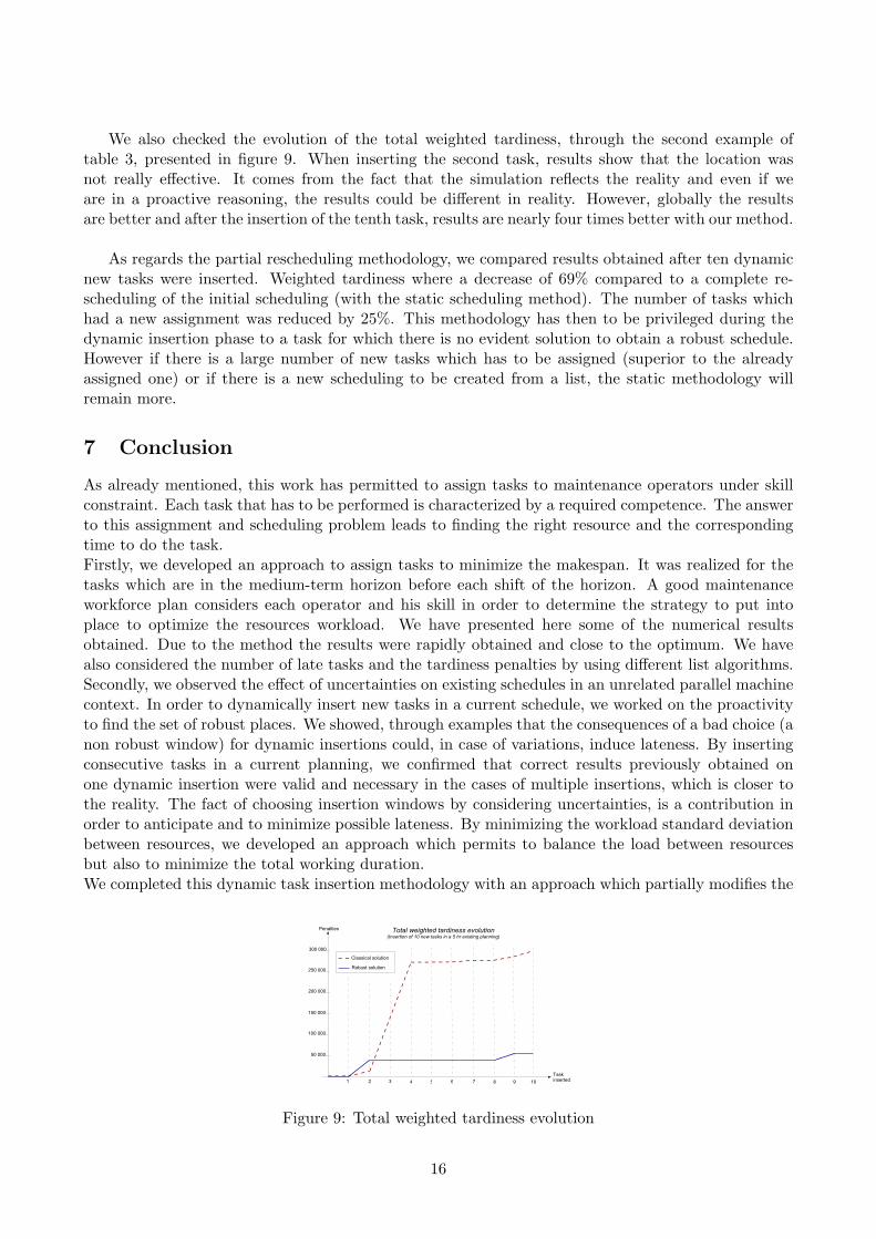
We also checked the evolution of the total weighted tardiness, through the second example oftable 3, presented in figure 9. When inserting the second task, results show that the location wasnot really effective. It comes from the fact that the simulation reflects the reality and even if weare in a proactive reasoning, the results could be different in reality. However, globally the resultsare better and after the insertion of the tenth task, results are nearly four times better with our method.

As regards the partial rescheduling methodology, we compared results obtained after ten dynamicnew tasks were inserted. Weighted tardiness where a decrease of 69% compared to a complete re-scheduling of the initial scheduling (with the static scheduling method). The number of tasks whichhad a new assignment was reduced by 25%. This methodology has then to be privileged during thedynamic insertion phase to a task for which there is no evident solution to obtain a robust schedule.However if there is a large number of new tasks which has to be assigned (superior to the alreadyassigned one) or if there is a new scheduling to be created from a list, the static methodology willremain more.

7 Conclusion

As already mentioned, this work has permitted to assign tasks to maintenance operators under skillconstraint. Each task that has to be performed is characterized by a required competence. The answerto this assignment and scheduling problem leads to finding the right resource and the correspondingtime to do the task.Firstly, we developed an approach to assign tasks to minimize the makespan. It was realized for thetasks which are in the medium-term horizon before each shift of the horizon. A good maintenanceworkforce plan considers each operator and his skill in order to determine the strategy to put intoplace to optimize the resources workload. We have presented here some of the numerical resultsobtained. Due to the method the results were rapidly obtained and close to the optimum. We havealso considered the number of late tasks and the tardiness penalties by using different list algorithms.Secondly, we observed the effect of uncertainties on existing schedules in an unrelated parallel machinecontext. In order to dynamically insert new tasks in a current schedule, we worked on the proactivityto find the set of robust places. We showed, through examples that the consequences of a bad choice (anon robust window) for dynamic insertions could, in case of variations, induce lateness. By insertingconsecutive tasks in a current planning, we confirmed that correct results previously obtained onone dynamic insertion were valid and necessary in the cases of multiple insertions, which is closer tothe reality. The fact of choosing insertion windows by considering uncertainties, is a contribution inorder to anticipate and to minimize possible lateness. By minimizing the workload standard deviationbetween resources, we developed an approach which permits to balance the load between resourcesbut also to minimize the total working duration.We completed this dynamic task insertion methodology with an approach which partially modifies the

Figure 9: Total weighted tardiness evolution

16

existing scheduling. It enables to improve the solution concerning weighted lateness by moving sometasks which have been compared to the static heuristic and shows that it gives comparable results.It has mainly for interest to reduce the employees disturbances in the case of too frequent changes ofschedule.

References

[1] Adolfo Crespo-Marquez and Jatinder N.D. Gupta. Contemporary maintenance management:process, framework and supporting pillars. Omega, 36:313–326, 2006.

[2] S.L. Van de Velde. Duality-based algorithms for scheduling unrelated parallel machines. ORSAJournal of Computing, 5:192–205, 1993.

[3] Carl Esswein, Jean-Charles Billaut, and V.-A. Strusevich. Two-machine shop scheduling: com-promise between flexibility and makespan value. In European Journal of Operational Research,2005.

[4] B. Grabot and A. Letouzey. Short-term manpower management in manufacturing systems : newrequirement and dss prototyping. Computers in Industry, 43:11–29, 2000.

[5] A. Hariri and C. N. Potts. Heuristics for scheduling unrelated parallel machines. Computers &Operations Research, 18(3):323–331, 1991.

[6] O. Ibarra and C. Kim. Heuristic algorithms for scheduling independent tasks of non identicalprocessors. Journal of the Association for Computing Machinery, 24:280–289, 1977.

[7] J. K. Lenstra, D. B. Shmoys, and E. Tardos. Approximation algorithms for scheduling unrelatedmachines. Mathematical programming, 46:259–271, 1990.

[8] Silvano Martello, Francois Soumis, and Paolo Toth. Exact and approximation algorithms formakespan minimisation on unrelated parallel machines. Discrete Applied Mathematics, 75:169–188, 1997.

[9] E. Mokotoff and P.Chretienne. A cutting plane algorithm for the unrelated parallel machinescheduling problem. European Journal of Operational Research, 141:515–525, 2002.

[10] Michele Pfund, John W. Fowler, and Jatinder N. D. Gupta. A survey of algorithms for singleand multi-objective unrelated machine deterministic scheduling problems. Journal of the ChineseInstitute of Industrial Engineers, 21(3):230–241, 2004.

[11] Mickael Pinedo. Scheduling, Theory, Algorithms and Systems. Prentice, 1995.

[12] H.A. Simon. Administrative behaviour: a study of Decision Making Processes in AdministrativeOrganizations. Mac Millan, New York, 1947.

17