Statistical Adjustments to

Engineering Models

V. ROSHAN JOSEPH∗and SHREYES N. MELKOTE†

Georgia Institute of Technology, Atlanta, GA 30332

Abstract

Statistical models are commonly used in quality improvement studies. However,

such models tend to perform poorly when predictions are made away from the observed

data points. On the other hand, engineering models derived using the underlying

physics of the process do not always match satisfactorily with reality. This article

proposes engineering-statistical models that overcomes the disadvantages of engineering

models and statistical models. The engineering-statistical model is obtained through

some adjustments to the engineering model using experimental data. The adjustments

are done in a sequential way and are based on empirical Bayes methods. We also

develop approximate frequentist procedures for adjustments that are computationally

much easier to implement. The usefulness of the methodology is illustrated using a

problem of predicting surface roughness in a micro-cutting process and the optimization

of a spot welding process.

Key Words: Bayesian methods; Calibration; Computer experiments; Gaussian process; Pre-

diction; Semi-empirical models; Validation.

∗Dr. Joseph is an Associate Professor in the H. Milton Stewart School of Industrial and Systems Engi-

neering at Georgia Tech. He is a Member of ASQ. His email address is roshan@gatech.edu.†Dr. Melkote is a Professor in the George W. Woodruff School of Mechanical Engineering at Georgia

Tech. His email address is smelkote@gatech.edu.

1

Introduction

Models describing the performance of a physical process are essential for prediction, control,

and optimization. In general, there are two approaches for developing models. One approach

is to develop models based on the engineering/physical laws governing the process, which

include analytical models and finite element models. We call such models engineering mod-

els. For example, in a metal cutting process, an analytical model can be developed using

the slip line field method for the analysis of stresses and strains induced in the material

during the cutting (Oxley 1989). A finite element model for the same process can also be

developed, which accounts for the process geometry/kinematics and the intricate physics of

finite material deformation during cutting (Marusich and Ortiz 1995). Another approach to

develop models is to postulate statistical models and estimate them based on the data gen-

erated from the process. Although engineering models are quite common in product design

(Santner, Williams, and Notz 2003), statistical models are more commonly used in quality

improvement (Wu and Hamada 2000).

Both modeling approaches have drawbacks. Predictions derived from engineering models

are often not accurate. This is because engineering models are developed based on several

simplifying assumptions, which may not hold true in practice. On the other hand, statistical

models can give good prediction at points close to the observed data. However, when trying

to predict in regions away from data, predictions can be poor and may at times make

no physical sense. Moreover, the experimental data required for estimating the statistical

models can be expensive.

Our objective is to develop a modeling approach that utilizes both engineering models

and statistical models. We term such models engineering-statistical models. This approach

combines the advantages of the two models and thus, mitigates their individual drawbacks.

Engineering-statistical models are expected to produce more realistic predictions than engi-

neering models and are less expensive to estimate than statistical models.

To illustrate the idea, consider the problem of predicting surface roughness as a function

of feed in a micro-cutting process. Figure 1 shows an illustration of a turning operation

2

Workpiece

ToolPrimary cutting edge

Feed (x)

Secondary cutting edge

Ykinematic

Nose radius (rn)

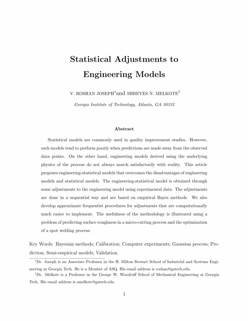
Figure 1: Illustration of turning operation showing surface roughness.

(adapted from Shaw 1997). As can be seen in the figure, the waveform left on the finished

surface is mainly due to the tool nose geometry and feed. An analytical model for the peak-

to-valley surface roughness (Y ) considering only the kinematics of machining is given by

(Shaw 1997)

Ykinematic =x2

8rn, (1)

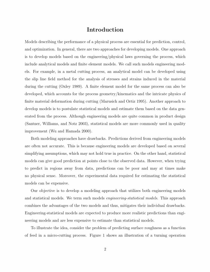
where x is the feed (in microns/revolution) and rn is the tool nose radius (in microns). Figure

2 shows the surface roughness data obtained from micro-turning of an aluminium alloy using

a diamond tool with nose radius of 800 microns (Liu and Melkote 2006). Clearly, the predic-

tions of the engineering model (dashed line) are poor. Now consider the statistical modeling

approach. Suppose that we have data only up to x = 20. A quadratic model is fitted to the

data and is also shown in the figure (dotted line). We can see that although the statistical

model is useful for predicting surface roughness in the range 5-20 microns/revolution, it be-

haves poorly outside this range. An engineering-statistical model is also fitted using the data

with x ≤ 20 and is shown in the figure (solid line). The details of the model and estimation

will be given later. Clearly, the engineering-statistical model is much better than both the

engineering model and the statistical model. Note that the statistical model gave the best fit

to the data, but seems to be the worst among the three models. The engineering-statistical

3

model came out as the best model because it behaves like the engineering model and is also

close to the data. This provides the intuition that statistical adjustments to the engineering

model should be made in such a way that they bring the engineering model closer to the

data by making minimal changes to it.

20 40 60 80 100

01

23

45

6

feed (x)

surf

ace

roug

hnes

s

Engineering model

Statistical model Engineering−Statistical model

Figure 2: Comparison of different models. The statistical model and the engineering-

statistical model are fitted using data for which feed ≤ 20.

The basic idea of improving engineering models using experimental data is not new. The

so-called mechanistic models are obtained by estimating the unknown parameters (known

as calibration parameters) in the engineering model from real data (see, for examples, Box

and Hunter 1962, Kapoor et al. 1998). However, such models are not general. For example,

there can be an engineering model with no calibration parameters and thus, the mechanistic

modeling approach cannot be used. Moreover, such models do not correct for model in-

adequacy. Kennedy and O’Hagan (2001) proposed a model using Gaussian process that is

capable of accounting for the model inadequacy. Other recent work in this area include Reese

et al. (2004), Higdon et al. (2004), Bayarri et al. (2007), and Qian and Wu (2008). Our

approach for developing engineering-statistical models is built on this earlier work. However,

our approach differs in terms of the modeling and estimation, which will be explained in later

sections.

4

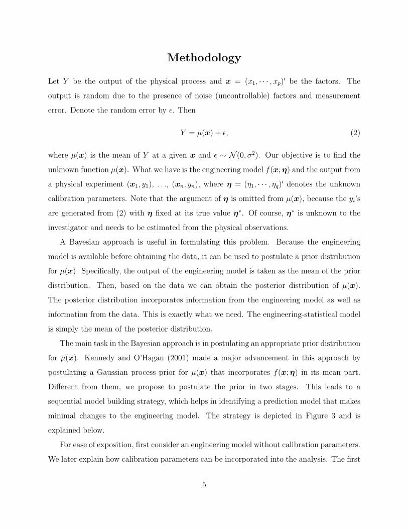
Methodology

Let Y be the output of the physical process and x = (x1, · · · , xp)′ be the factors. The

output is random due to the presence of noise (uncontrollable) factors and measurement

error. Denote the random error by ε. Then

Y = µ(x) + ε, (2)

where µ(x) is the mean of Y at a given x and ε ∼ N (0, σ2). Our objective is to find the

unknown function µ(x). What we have is the engineering model f(x;η) and the output from

a physical experiment (x1, y1), . . ., (xn, yn), where η = (η1, · · · , ηq)′ denotes the unknown

calibration parameters. Note that the argument of η is omitted from µ(x), because the yi’s

are generated from (2) with η fixed at its true value η∗. Of course, η∗ is unknown to the

investigator and needs to be estimated from the physical observations.

A Bayesian approach is useful in formulating this problem. Because the engineering

model is available before obtaining the data, it can be used to postulate a prior distribution

for µ(x). Specifically, the output of the engineering model is taken as the mean of the prior

distribution. Then, based on the data we can obtain the posterior distribution of µ(x).

The posterior distribution incorporates information from the engineering model as well as

information from the data. This is exactly what we need. The engineering-statistical model

is simply the mean of the posterior distribution.

The main task in the Bayesian approach is in postulating an appropriate prior distribution

for µ(x). Kennedy and O’Hagan (2001) made a major advancement in this approach by

postulating a Gaussian process prior for µ(x) that incorporates f(x;η) in its mean part.

Different from them, we propose to postulate the prior in two stages. This leads to a

sequential model building strategy, which helps in identifying a prediction model that makes

minimal changes to the engineering model. The strategy is depicted in Figure 3 and is

explained below.

For ease of exposition, first consider an engineering model without calibration parameters.

We later explain how calibration parameters can be incorporated into the analysis. The first

5

Check & Correct

No

Is MIlarge?

Functional Adjustment Model

Yes

No

Yes

No Engineering Model

Constant adjustment

Useful?

Is MIlarge?

Constant Adjustment Model

Yes

Engineering Model

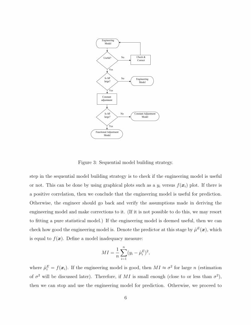
Figure 3: Sequential model building strategy.

step in the sequential model building strategy is to check if the engineering model is useful

or not. This can be done by using graphical plots such as a yi versus f(xi) plot. If there is

a positive correlation, then we conclude that the engineering model is useful for prediction.

Otherwise, the engineer should go back and verify the assumptions made in deriving the

engineering model and make corrections to it. (If it is not possible to do this, we may resort

to fitting a pure statistical model.) If the engineering model is deemed useful, then we can

check how good the engineering model is. Denote the predictor at this stage by µE(x), which

is equal to f(x). Define a model inadequacy measure:

MI =1

n

n∑i=1

(yi − µEi )2,

where µEi = f(xi). If the engineering model is good, then MI ≈ σ2 for large n (estimation

of σ2 will be discussed later). Therefore, if MI is small enough (close to or less than σ2),

then we can stop and use the engineering model for prediction. Otherwise, we proceed to

6

make statistical adjustments.

First we do a simple location-scale adjustment:

µ(x)− f(x) = β0 + β1(f(x)− f),

where f =∑n

i=1 f(xi)/n. The prior for µ(x) is postulated through the parameters: β0 ∼

N (0, τ 20 ) and β1 ∼ N (0, τ 2

1 ), where β0 and β1 are independent. Note that the mean of µ(x)

is f(x). We call this a constant adjustment model, because two constants are used for the

adjustments. The predictor at this stage is denoted by µC(x) = f(x) + β0 + β1(f(x) − f).

We again compute the model inadequacy measure:

MI =1

n

n∑i=1

(yi − µCi )2,

where µCi = f(xi) + β0 + β1(f(xi) − f) and βj denotes the estimate of βj from the data.

If MI is small enough (close to or less than σ2), we stop and use the constant adjustment

model for prediction. Otherwise, we proceed to make a more sophisticated adjustment to

the engineering model.

Let

µ(x)− µC(x) = δ(x;α),

where δ(x;α) is used for capturing the inadequacy of the constant adjustment model. We

call this a functional adjustment model, because the functional form of the predictor is

different from the engineering model. The form of the function δ is obtained using residual

analysis from the constant adjustment model. A simple method is to use a linear model

given by δ(x;α) =∑m

i=0 αiui(x), where ui’s are known functions in x. The prior for α is

chosen to make E(δ(x;α)) = 0. Thus, we must have E(α) = 0 in the linear model. Now,

µC(x) and α can be estimated from data. The functional adjustment predictor is given by

µF (x) = µC(x) + δ(x; α). Although simultaneously estimating µC(x) and α from the data

may lead to better fitting, we propose to do it in two stages, i.e., use the estimate of µC(x)

from the previous stage and estimate only α in the current stage. This two-stage estimation

procedure reduces the tendency for the statistical model to replace the engineering model

7

by forcing it to be present in the final predictor. This may not give the best fit in terms

of the observed data, but as illustrated in Figure 2, it may give a better prediction at the

unobserved points. Moreover, it helps in avoiding certain identifiability problems and makes

the computations much simpler.

The functional adjustment model is closely related to the model in Kennedy and O’Hagan

(2001). Their model can be written as µ(x) = ρ0 + ρ1f(x) + δ(x), where f(x) and δ(x) are

assumed to be independent Gaussian processes. A Gaussian process prior is used for f(x)

because the engineering model is assumed to be computationally intensive to evaluate and

could be observed only at some finite locations. First, following the suggestion of Bayarri et

al. (2007), we do not use physical data to estimate f(x). Therefore, we only need to consider

models for given f(x). When f(x) is complex, it will be replaced by an easy-to-evaluate

metamodel (a model that approximates f(x)). Apart from the two-stage fitting of the

functional adjustment model, there are other differences in our approach compared to that

of Kennedy and O’Hagan. The prior specification in our model is quite different. Kennedy

and O’Hagan assume independent and improper priors for ρ0 and ρ1, whereas because of the

reparameterization, we use dependent and proper priors for these two parameters. Different

from the Gaussian process model, we use a linear/nonlinear regression model for δ(x). This

enables us to identify important factors affecting the model discrepancy through variable

selection and use minimal adjustments to the engineering model. This agrees with our

overall objective of identifying a simple adjustment model, which is a major difference from

the Kennedy and O’Hagan’s approach.

The unknown calibration parameters (η) can be easily incorporated into the sequential

model building strategy by treating them as hyperparameters. This is quite legitimate be-

cause η enters the Bayesian model only through f(x;η), which is taken as the mean of the

prior distribution of µ(x). We start the procedure with a least squares estimate of η and

in the next stage obtain an empirical Bayes estimate from the constant adjustment model.

Because η does not appear in δ(x;α), the fitting of functional adjustment model remains

the same as before. This approach is markedly different from the previous approaches (see,

Kennedy and O’Hagan 2001, Bayarri et al. 2007), wherein η and δ are simultaneously

8

estimated from the data. Researchers have pointed out identifiability problems with such

an approach and associated convergence problems with Markov chain Monte Carlo imple-

mentation (see, e.g., Loeppky, Bingham, and Welch 2006). This identifiability problem is

completely avoided by virtue of our two-stage fitting procedure.

Note that Kennedy and O’Hagan (2001) and others directly fit the functional adjustment

model, but we do it only at the last stage of our sequential model building strategy and only

if it is necessary. This is because, a functional adjustment model may completely change the

basic shape of the engineering model. Such a major change should be considered necessary

only when the constant adjustment model is not working well. To draw an analogy, a surgery

may be considered for treatment only when the patient is not satisfactorily responding to

the prescribed drugs.

We use empirical Bayes methods for estimation of the models and derive explicit ex-

pressions for some of the results. This makes our approach much easier to implement than

the procedures in Kennedy and O’Hagan (2001), Reese et al. (2004), Higdon et al. (2004),

Bayarri et al. (2007), and Qian and Wu (2008). We also develop approximate frequentist

procedures to our empirical Bayes approach, which are computationally very efficient and

should appeal to many practitioners. Of course, there is no free lunch; we admit that un-

certainties about the hyperparameters are not accounted for in our approach and therefore,

the prediction intervals are not as accurate as those obtained by using hierarchical Bayes

methods.

In the next two sections, we explain the details of fitting constant and functional adjust-

ment models.

Constant Adjustment Model

To make the exposition simple, consider first an engineering model with no calibration pa-

rameters. The details of the adjustments when calibration parameters are present will be

9

discussed later. The constant adjustment model is given by

Y − f(x) = β0 + β1(f(x)− f) + ε,

where ε ∼ N (0, σ2), β0 ∼ N (0, τ 20 ), β1 ∼ N (0, τ 2

1 ), and they are independent. For the

moment, assume that σ2 is known.

We have the data (x1, y1), . . . , (xn, yn). Let y = (y1, . . . , yn)′, β = (β0, β1)′, and ε =

(ε1, . . . , εn)′. Let F be an n× 2 matrix, whose first column is a column of 1’s and the second

column is (f1 − f , . . . , fn − f)′ and f = (f1, . . . , fn)′, where f(xi) = fi. Then, the constant

adjustment model can be written as

y − f = Fβ + ε, ε ∼ N (0, σ2I), β ∼ N (0,Σ), (3)

where 0 is a vector of 0’s, I is the n-dimensional identity matrix, and Σ = diag{τ 20 , τ

21 }. The

posterior distribution of β is given by

β|y ∼ N((F ′F + σ2Σ−1)−1F ′(y − f), σ2(F ′F + σ2Σ−1)−1

). (4)

Denote the posterior mean of β by β = (F ′F + σ2Σ−1)−1F ′(y − f). Then, the constant

adjustment predictor is given by

µC(x) = f(x) + β0 + β1(f(x)− f). (5)

The formulas can be simplified. Let β = (F ′F )−1F ′(y − f), which is the least squares

estimate of β. We obtain

β0 = y − f and β1 =n∑i=1

(yi − fi)(fi − f)/S, (6)

where S =∑n

i=1(fi − f)2. Then,

β0 =τ 20

τ 20 + σ2/n

β0 and β1 =τ 21

τ 21 + σ2/S

β1. (7)

Thus, β0 and β1 are shrinkage estimates of their least squares estimates.

10

If the model inadequacy measure MI for the constant adjustment model is small, then

it can be used for prediction. The (1− α)-Bayesian prediction interval is given by

µC(x)± zα/2σ{

1 +1

n+ σ2/τ 20

+(f(x)− f)2

S + σ2/τ 21

}1/2

, (8)

where zα/2 is the (1− α/2)-quantile of the standard normal distribution. Note that we had

assumed the engineering model to be known. However, in some cases the engineering model

can be quite complex and observable only at some finite locations. As mentioned before,

in such cases the predictions can be made by replacing f(x) with a metamodel f(x), i.e.,

µC(x) = f(x) + β0 + β1(f(x) − f). However, the prediction interval needs to be modified

to account for the uncertainty in the metamodel. Let v(x) denote the prediction variance

of the metamodel at the location x. Assume that the engineering model evaluations are

available at the locations of the physical experiment. Then, as shown in the Appendix, an

approximate prediction interval is given by

µC(x)± zα/2σ{

1 +1

n+ σ2/τ 20

+(f(x)− f)2 + v(x)

S + σ2/τ 21

+ (1 + β1)2v(x)

}1/2

. (9)

Of course, the predictions can be made only after specifying the values of σ2, τ 20 , and

τ 21 . First consider the case of σ2. It can be estimated from replicates and prior knowledge.

Suppose that we have r replicates at d distinct values of x. Thus, n = rd. Let yij be the jth

replicate in the ith group, i = 1, . . . , d and j = 1, . . . , r. Let s2i =

∑rj=1(yij−yi)2/(r−1) be the

sample variance of the ith group and s2 =∑d

i=1 s2i /d the pooled variance. Assume an inverse

gamma prior distribution for σ2 with parameters ν/2 and νσ20/2, where σ2

0 is an estimate of

σ2 from the prior knowledge (which could come from gage repeatability and reproducibility

studies and experience with the product/process) and ν controls its uncertainty. Then, σ2|s2

also has an inverse gamma distribution with parameters (d(r − 1) + ν)/2 and (d(r − 1)s2 +

νσ20)/2. Therefore, σ2 can be estimated by

σ2 =d(r − 1)s2 + νσ2

0

d(r − 1) + ν, (10)

which is a weighted average of s2 and σ20 (This estimate lies between the posterior mean and

posterior mode of σ2|s2 and thus is closer to the posterior median). However, after obtaining

11

this estimate we act as though it was known. In other words, we assume d(r − 1) + ν to be

large enough to neglect the uncertainty of σ2 in the subsequent inference.

The hyperparameters τ 20 and τ 2

1 can be estimated from data using empirical Bayes

methods. By integrating out β from (3), we obtain the marginal distribution of y as

N (f ,FΣF ′ + σ2I). Thus, the marginal log-likelihood is given by

l = −1

2log det(FΣF ′ + σ2I)− 1

2(y − f)′(FΣF ′ + σ2I)−1(y − f), (11)

where the constant term is omitted. Now l can be maximized with respect to τ 20 and τ 2

1 to

obtain their estimates.

We can derive explicit expressions for the maximum likelihood estimates. It can be shown

that maximizing l with respect to τ 20 and τ 2

1 is equivalent to minimizing

log(nτ 20 + σ2) + log(τ 2

1S + σ2) +nβ2

0

nτ 20 + σ2

+Sβ2

1

τ 21S + σ2

.

Under the nonnegativity constraints τ 20 ≥ 0 and τ 2

1 ≥ 0, we obtain

τ 20 =

(β2

0 − σ2/n)

+and τ 2

1 =(β2

1 − σ2/S)

+, (12)

where (x)+ = x if x > 0 and 0 otherwise. Substituting in (7), we obtain

β0 =

(1− 1

z20

)+

β0 and β1 =

(1− 1

z21

)+

β1, (13)

where

z0 =β0

σ/√n

and z1 =β1

σ/√S. (14)

Thus, βj is shrunk to 0 when |zj| ≥ 1. Note that zj is the test statistic for testing the

hypotheses H0 : βj = 0. Thus, although we started with a Bayesian approach, the final

results are close to a frequentist approach. As shown by Joseph and Delaney (2008), the

best approximated version of the frequentist testing to the Bayesian shrinkage estimation

uses a critical value of√

2. This amounts to making the shrinkage coefficient (1 − 1/z2j )+

equal to 0 when the shrinkage coefficient is less than 1/2 and 1 otherwise. Thus, to obtain a

constant adjustment model, we may use simple linear regression to fit yi− fi = β0 + β1(fi−

12

f) + εi and force βj to be 0 if |zj| <√

2. This clearly shows the simplicity of the proposed

approach. Because of its simplicity and ease of implementation, which will be more evident

from the next section, we recommend using the frequentist approach over the empirical Bayes

approach.

By letting τ 20 and τ 2

1 go to ∞ in (8), we obtain the familiar prediction interval for the

frequentist approach given by

µC(x)± zα/2σ{

1 +1

n+

(f(x)− f)2

S

}1/2

. (15)

Note that if any of the coefficients is truncated to 0, then the corresponding term in the

prediction variance should be removed (note that 1/n and (f(x) − f)2/S correspond to β0

and β1, respectively). The approximate prediction interval that incorporates the uncertainty

in the metamodel can be obtained from (9) as

µC(x)± zα/2σ{

1 +1

n+

(f(x)− f)2 + v(x)

S+ (1 + β1)

2v(x)

}1/2

, (16)

where β1 = β1 if |z1| <√

2 and 0 otherwise.

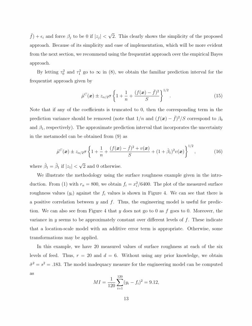
We illustrate the methodology using the surface roughness example given in the intro-

duction. From (1) with rn = 800, we obtain fi = x2i /6400. The plot of the measured surface

roughness values (yi) against the fi values is shown in Figure 4. We can see that there is

a positive correlation between y and f . Thus, the engineering model is useful for predic-

tion. We can also see from Figure 4 that y does not go to 0 as f goes to 0. Moreover, the

variance in y seems to be approximately constant over different levels of f . These indicate

that a location-scale model with an additive error term is appropriate. Otherwise, some

transformations may be applied.

In this example, we have 20 measured values of surface roughness at each of the six

levels of feed. Thus, r = 20 and d = 6. Without using any prior knowledge, we obtain

σ2 = s2 = .183. The model inadequacy measure for the engineering model can be computed

as

MI =1

120

120∑i=1

(yi − fi)2 = 9.12,

13

0.0 0.5 1.0 1.5

2.5

3.0

3.5

4.0

4.5

5.0

5.5

6.0

f

y

Figure 4: Plot of y against f in the surface roughness example.

which is much larger than σ2 and therefore, the engineering model is not adequate.

A hypothesis test can be performed to check this. Because the engineering model is

deterministic fij = fi. for all j = 1, . . . , r. Let µi. be the true mean value for the ith group,

i = 1, . . . , d. Then, testing the adequacy of the engineering model can be formulated as

H0 : µi. = fi. against H1 : µi. 6= fi., i = 1, . . . , d. Now, H0 can be rejected if∑d

i=1(yi−fi.)2 >

σ2/rχ2d,α, where χ2

d,α is the upper α-quantile of the χ2d distribution. This can be written in

terms of MI as

MI >r − 1

rs2 +

σ2

nχ2d,α.

Note that when σ2 is not known, it should be replaced with σ2. At α = .05, 19/20× .183 +

.183/120 × 12.59 = .193 < MI, which confirms that the engineering model is not good for

prediction. Hence we proceed to fit the constant adjustment model.

Using a simple linear regression for y − f(x) on f(x) − f , we obtain β0 = 2.98 and

β1 = −.11. From (14), |z0| = 2.98/√.183/120 = 76.2 and |z1| = .11/

√.183/39.1 = 1.60.

Thus, the empirical Bayes method gives µC(x) − f(x) = 2.98 − .07(f(x) − .4857), whereas

the frequentist approximation gives

µC(x)− f(x) = 2.98− .11(f(x)− .4857). (17)

14

20 40 60 80 100

01

23

45

6

x

y

Engineering model

Constant adjustment model

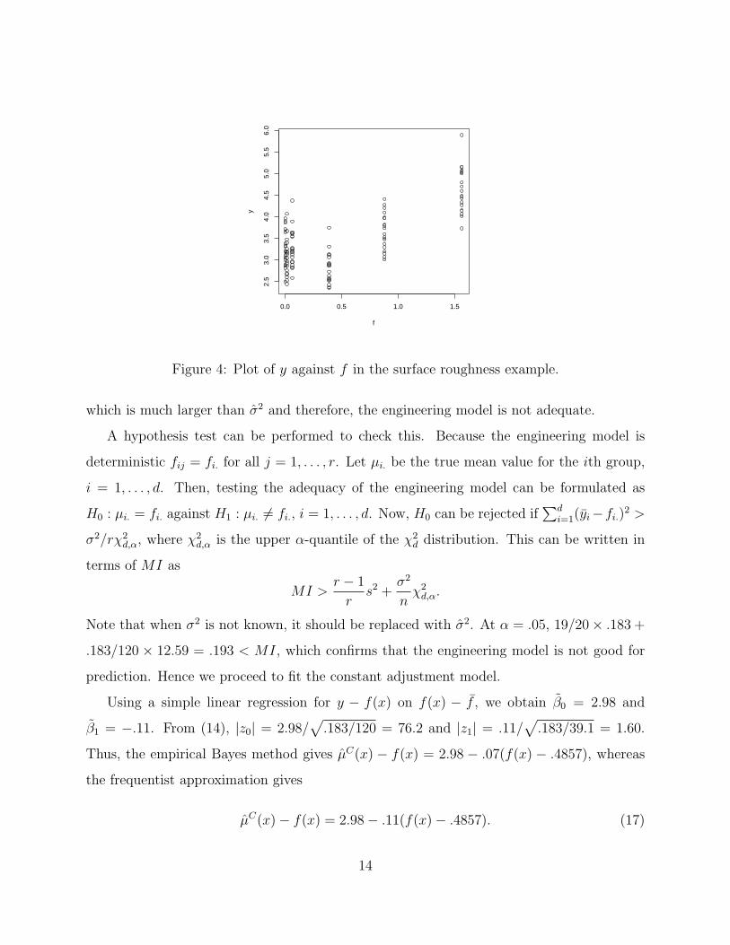
Figure 5: Constant adjustment model in the surface roughness example.

Hereafter, we use the model obtained through frequentist approximation.

A plot of the predictor is shown in Figure 5, which clearly shows great improvement

compared to the engineering model. To quantify the performance, we can compute the

model inadequacy measure for the constant adjustment model as

MI =1

120

120∑i=1

(yi − µCi )2 = .255.

This is much smaller than the engineering model and only slightly larger than σ2 = .183,

showing that the constant adjustment model has greatly improved the prediction. If the

constant adjustment model is true, then∑d

i=1(yi − µCi. )2/(σ2/r) follows a χ2d−2 distribution

(χ2d−1 if β0 or β1 is truncated to 0). Therefore, the constant adjustment model is inadequate

if

MI >r − 1

rs2 +

σ2

nχ2d−2,α.

Note that if we replace σ2 with s2 and use the approximation χ2d−2,α ≈ (d − 2)Fd−2,d(r−1),α,

then the above test reduces to the well known lack-of-fit test in regression analysis (see, e.g.,

Neter et al. 1996, page 123). The two tests are approximately the same when d(r − 1) is

large. We obtain at α = .05, 19/20 × .183 + .183/120 × 9.49 = .188 < MI, and thus, the

15

constant adjustment model still has some model inadequacy. Therefore, we proceed to fit a

functional adjustment model.

Functional Adjustment Model

The functional adjustment model is given by

Y − µC(x) = δ(x;α) + ε,

where ε ∼ N (0, σ2), δ(x;α) captures the discrepancy between the observations and the

constant adjustment model, and α is a set of unknown parameters. Kennedy and O’Hagan

(2001) proposed using a Gaussian process prior for the model inadequacy term in their model.

Such priors are popular in the analysis of deterministic computer experiments (see Sacks et

al. 1989). However, the data from the physical process are corrupted by random errors and

therefore, there is no compelling reason to use such priors in this problem. A more common

approach is to use linear and nonlinear regression models.

Consider a linear model

δ(x;α) = α0 +m∑i=1

αiui(x), (18)

where ui(x)’s are known functions of x and α = (α0, . . . , αm)′ are unknown parameters.

Center the ui’s such that∑n

j=1 ui(xj) = 0. Now we can put a prior on α, say α ∼ N (0, γ2R)

(see Joseph 2006a, Joseph and Delaney 2007). As discussed before, we use µC(x) from the

previous stage and estimate only α at this stage. Let µC be the fitted values from the

constant adjustment model and U be the n× (m+ 1) model matrix corresponding to (18),

i.e., the first column of U is a column of 1’s and the other m columns correspond to the

ui(x)’s which take values depending on the n data points. Then, the functional adjustment

predictor is given by

µF (x) = µC(x) +m∑i=0

αiui(x), (19)

where µC(x) is given in (5) and

α = (U ′U +σ2

γ2R−1)−1U ′(y − µC).

16

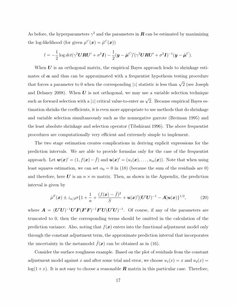
As before, the hyperparameters γ2 and the parameters in R can be estimated by maximizing

the log-likelihood (for given µC(x) = µC(x))

l = −1

2log det(γ2URU ′ + σ2I)− 1

2(y − µC)′(γ2URU ′ + σ2I)−1(y − µC).

When U is an orthogonal matrix, the empirical Bayes approach leads to shrinkage esti-

mates of α and thus can be approximated with a frequentist hypothesis testing procedure

that forces a parameter to 0 when the corresponding |z| statistic is less than√

2 (see Joseph

and Delaney 2008). When U is not orthogonal, we may use a variable selection technique

such as forward selection with a |z| critical value-to-enter as√

2. Because empirical Bayes es-

timation shrinks the coefficients, it is even more appropriate to use methods that do shrinkage

and variable selection simultaneously such as the nonnegative garrote (Breiman 1995) and

the least absolute shrinkage and selection operator (Tibshirani 1996). The above frequentist

procedures are computationally very efficient and extremely simple to implement.

The two stage estimation creates complications in deriving explicit expressions for the

prediction intervals. We are able to provide formulas only for the case of the frequentist

approach. Let w(x)′ = (1, f(x)− f) and u(x)′ = (u1(x), . . . , um(x)). Note that when using

least squares estimation, we can set α0 = 0 in (18) (because the sum of the residuals are 0)

and therefore, here U is an n×m matrix. Then, as shown in the Appendix, the prediction

interval is given by

µF (x)± zα/2σ{1 +1

n+

(f(x)− f)2

S+ u(x)′[(U ′U)−1 −A]u(x)}1/2, (20)

where A = (U ′U)−1U ′F (F ′F )−1F ′U(U ′U)−1. Of course, if any of the parameters are

truncated to 0, then the corresponding terms should be omitted in the calculation of the

prediction variance. Also, noting that f(x) enters into the functional adjustment model only

through the constant adjustment term, the approximate prediction interval that incorporates

the uncertainty in the metamodel f(x) can be obtained as in (16).

Consider the surface roughness example. Based on the plot of residuals from the constant

adjustment model against x and after some trial and error, we choose u1(x) = x and u2(x) =

log(1 + x). It is not easy to choose a reasonable R matrix in this particular case. Therefore,

17

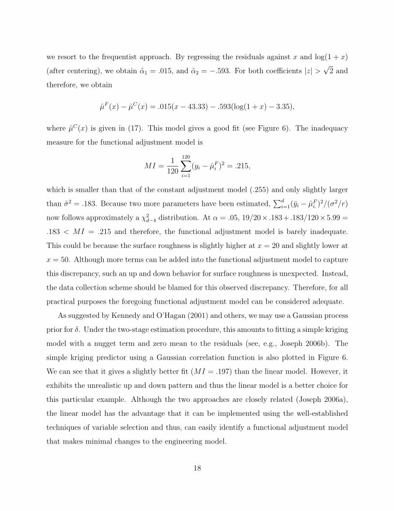
we resort to the frequentist approach. By regressing the residuals against x and log(1 + x)

(after centering), we obtain α1 = .015, and α2 = −.593. For both coefficients |z| >√

2 and

therefore, we obtain

µF (x)− µC(x) = .015(x− 43.33)− .593(log(1 + x)− 3.35),

where µC(x) is given in (17). This model gives a good fit (see Figure 6). The inadequacy

measure for the functional adjustment model is

MI =1

120

120∑i=1

(yi − µFi )2 = .215,

which is smaller than that of the constant adjustment model (.255) and only slightly larger

than σ2 = .183. Because two more parameters have been estimated,∑d

i=1(yi − µFi. )2/(σ2/r)

now follows approximately a χ2d−4 distribution. At α = .05, 19/20× .183+ .183/120×5.99 =

.183 < MI = .215 and therefore, the functional adjustment model is barely inadequate.

This could be because the surface roughness is slightly higher at x = 20 and slightly lower at

x = 50. Although more terms can be added into the functional adjustment model to capture

this discrepancy, such an up and down behavior for surface roughness is unexpected. Instead,

the data collection scheme should be blamed for this observed discrepancy. Therefore, for all

practical purposes the foregoing functional adjustment model can be considered adequate.

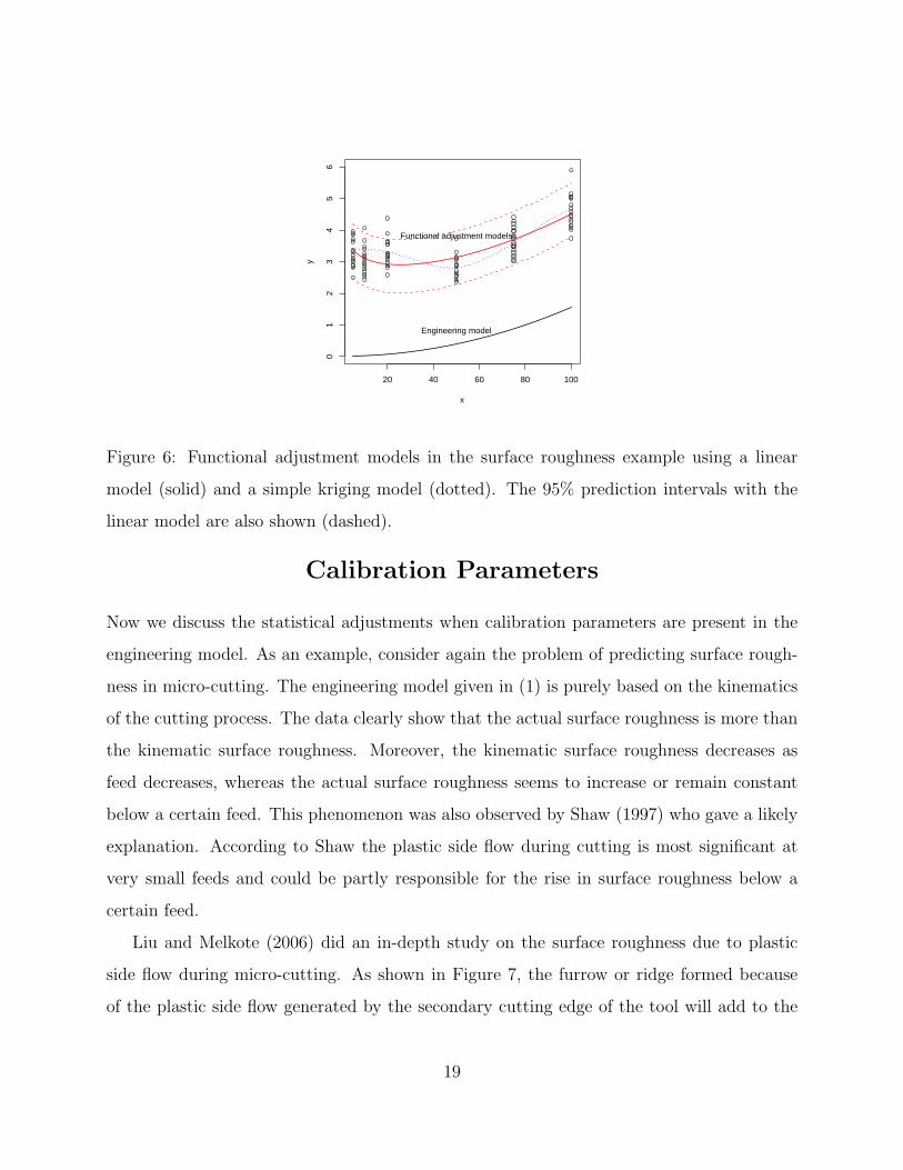
As suggested by Kennedy and O’Hagan (2001) and others, we may use a Gaussian process

prior for δ. Under the two-stage estimation procedure, this amounts to fitting a simple kriging

model with a nugget term and zero mean to the residuals (see, e.g., Joseph 2006b). The

simple kriging predictor using a Gaussian correlation function is also plotted in Figure 6.

We can see that it gives a slightly better fit (MI = .197) than the linear model. However, it

exhibits the unrealistic up and down pattern and thus the linear model is a better choice for

this particular example. Although the two approaches are closely related (Joseph 2006a),

the linear model has the advantage that it can be implemented using the well-established

techniques of variable selection and thus, can easily identify a functional adjustment model

that makes minimal changes to the engineering model.

18

20 40 60 80 100

01

23

45

6

x

y

Engineering model

Functional adjustment models

Figure 6: Functional adjustment models in the surface roughness example using a linear

model (solid) and a simple kriging model (dotted). The 95% prediction intervals with the

linear model are also shown (dashed).

Calibration Parameters

Now we discuss the statistical adjustments when calibration parameters are present in the

engineering model. As an example, consider again the problem of predicting surface rough-

ness in micro-cutting. The engineering model given in (1) is purely based on the kinematics

of the cutting process. The data clearly show that the actual surface roughness is more than

the kinematic surface roughness. Moreover, the kinematic surface roughness decreases as

feed decreases, whereas the actual surface roughness seems to increase or remain constant

below a certain feed. This phenomenon was also observed by Shaw (1997) who gave a likely

explanation. According to Shaw the plastic side flow during cutting is most significant at

very small feeds and could be partly responsible for the rise in surface roughness below a

certain feed.

Liu and Melkote (2006) did an in-depth study on the surface roughness due to plastic

side flow during micro-cutting. As shown in Figure 7, the furrow or ridge formed because

of the plastic side flow generated by the secondary cutting edge of the tool will add to the

19

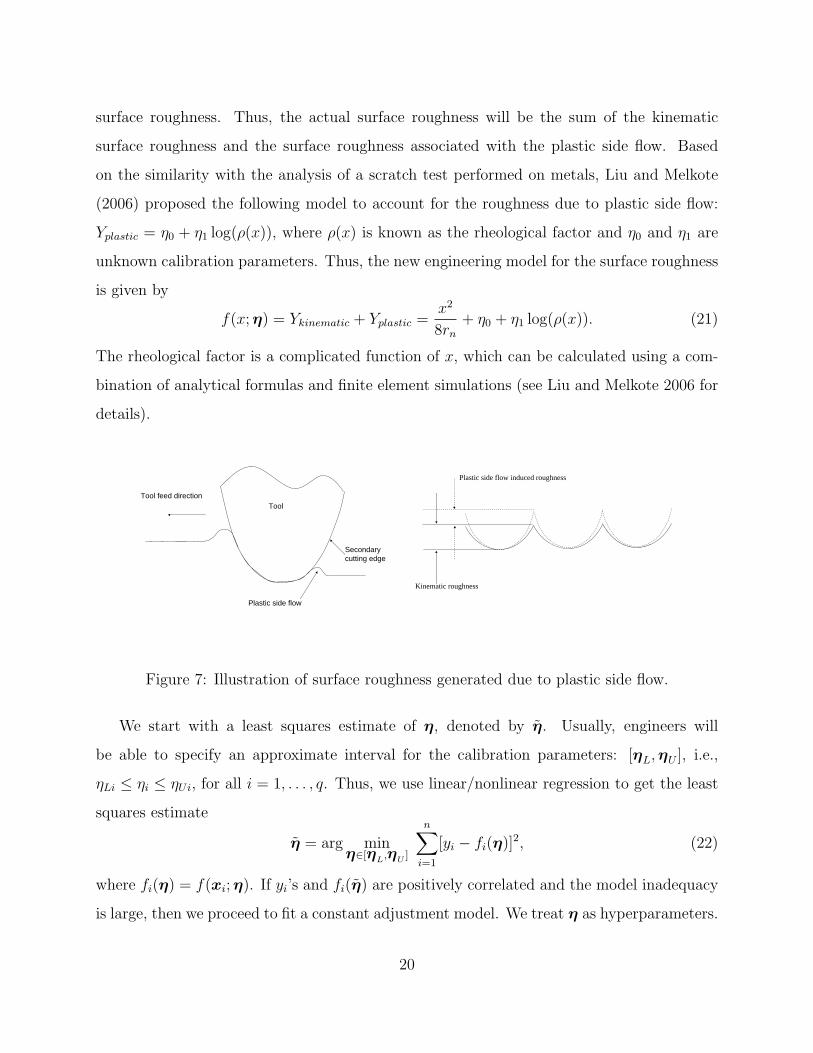
surface roughness. Thus, the actual surface roughness will be the sum of the kinematic

surface roughness and the surface roughness associated with the plastic side flow. Based

on the similarity with the analysis of a scratch test performed on metals, Liu and Melkote

(2006) proposed the following model to account for the roughness due to plastic side flow:

Yplastic = η0 + η1 log(ρ(x)), where ρ(x) is known as the rheological factor and η0 and η1 are

unknown calibration parameters. Thus, the new engineering model for the surface roughness

is given by

f(x;η) = Ykinematic + Yplastic =x2

8rn+ η0 + η1 log(ρ(x)). (21)

The rheological factor is a complicated function of x, which can be calculated using a com-

bination of analytical formulas and finite element simulations (see Liu and Melkote 2006 for

details).

Tool

Plastic side flow

Tool feed direction

Secondary cutting edge

Kinematic roughness

Plastic side flow induced roughness

Figure 7: Illustration of surface roughness generated due to plastic side flow.

We start with a least squares estimate of η, denoted by η. Usually, engineers will

be able to specify an approximate interval for the calibration parameters: [ηL,ηU ], i.e.,

ηLi ≤ ηi ≤ ηUi, for all i = 1, . . . , q. Thus, we use linear/nonlinear regression to get the least

squares estimate

η = arg minη∈[ηL,ηU ]

n∑i=1

[yi − fi(η)]2, (22)

where fi(η) = f(xi;η). If yi’s and fi(η) are positively correlated and the model inadequacy

is large, then we proceed to fit a constant adjustment model. We treat η as hyperparameters.

20

The constant adjustment model is given by

Y − f(x;η) = β0 + β1(f(x;η)− f(η)) + ε, (23)

where f(η) =∑n

i=1 fi(η)/n. As before β ∼ N (0,Σ) and ε ∼ N (0, σ2). Let f(η) =

(f1(η), · · · , fn(η))′ and define the model matrix F (η) similarly. Then, the hyperparameters

can be estimated by maximizing

l = −1

2log det(F (η)ΣF ′(η) + σ2I) (24)

−1

2(y − f(η))′(F (η)ΣF ′(η) + σ2I)−1(y − f(η)),

with respect to τ 20 , τ 2

1 , and η.

The foregoing optimization can be simplified as follows. First fix η and maximize l with

respect to τ 20 and τ 2

1 . We obtain

τ 20 (η) =

(β2

0(η)− σ2/n)

+and τ 2

1 (η) =(β2

1(η)− σ2/S(η))

+,

where βj(η) is the least squares estimate of βj and S(η) =∑n

i=1(fi(η)−f(η))2. Substituting

in (24), we obtain the profile log-likelihood of η. It is easy to show that maximizing the

profile log-likelihood is equivalent to minimizing

A(η) =1

σ2

n∑i=1

[yi − fi(η)]2 + log(nτ 20 (η) + σ2)

+ log(τ12(η)S(η) + σ2)− n2τ 2

0 (η)β20(η)

σ2(nτ 20 (η) + σ2)

− τ 21 (η)S2(η)β2

1(η)

σ2(τ 21 (η)S(η) + σ2)

.

After some simplification, we obtain (constant term omitted)

A(η) =1

σ2

n∑i=1

[yi − fi(η)]2 + log(1 + (z20(η)− 1)+) (25)

+ log(1 + (z21(η)− 1)+)− (z2

0(η)− 1)+ − (z21(η)− 1)+,

where z0(η) =√nβ0(η)/σ and z1(η) =

√S(η)β1(η)/σ. Now, by minimizing A(η) under

the constraints η ∈ [ηL,ηU ], we can obtain η. Then, the estimates of β0 and β1 can be

obtained as

β0 =

(1− 1

z20(η)

)+

β0(η) and β1 =

(1− 1

z21(η)

)+

β1(η). (26)

21

The foregoing empirical Bayes estimation is closely related to the following nonlinear

least squares estimation:

minβ0,β1,η

1

σ2

n∑i=1

[yi − fi(η)− β0 − β1(fi(η)− f(η))]2. (27)

By minimizing with respect to β0 and β1, we obtain

Q(η) =1

σ2

n∑i=1

[yi − fi(η)− β0(η)− β1(η)(fi(η)− f(η))]2

=1

σ2

n∑i=1

[yi − fi(η)]2 − z20(η)− z2

1(η). (28)

For large values of z20(η) and z2

1(η), A(η) behaves like Q(η) and therefore, minimizing A(η)

is approximately equivalent to minimizing Q(η). Thus, a frequentist version of the empirical

Bayes approach is to fit a nonlinear regression model yi = fi(η) + β0 + β1(fi(η)− f(η)) + εi

and truncate β0 and β1 to 0 if their |z| statistics are less than√

2. Note that if β0 = 0 and/or

β1 = 0, then η should be reestimated from the reduced model. This is quite intuitive and

very easy to implement. The implementation can be easily done using a standard statistical

software without requiring the need for additional programming work.

If the model inadequacy for the constant adjustment model is large, then we can proceed

to fit a functional adjustment model. As explained in the previous section, this can be done

by fitting a linear/nonlinear regression model to the residuals from the constant adjustment

model. By virtue of the two-stage estimation, we do not need to estimate η again. This

is extremely simple compared to the procedures in Kennedy and O’Hagan (2001), Bayarri

et al. (2007), and others. One could argue that because η is fixed at η when estimating

the functional adjustment model, we are not getting a good estimate of the true value of

the calibration parameters. However, since the functional form of the model is altered, the

calibration parameters lose their physical meaning and therefore the notion of “true” value

becomes questionable. Moreover, as shown by Loeppky et al. (2006), final prediction is not

affected much by η, because the errors in its estimation get compensated through the model

inadequacy part δ(x;α).

22

We explain the approach using the new surface roughness model. The rheological values

are computed using a combination of analytical formulas and finite element simulations for

the six values of feed as ρ(5) = 521, ρ(10) = 508, ρ(20) = 490, ρ(50) = 463, ρ(75) = 460,

and ρ(100) = 475. First we use the least squares method to obtain an initial estimate of η.

In this example, this can be easily done by using a simple linear regression for y − x2/(8r)

against log(ρ(x)). We obtain η = (−27.1, 4.86)′. The model inadequacy measure can be

computed as MI = .209, which is very small compared to the kinematic surface roughness

model (MI = 9.12). Thus, the new surface roughness model that includes the effect of

plastic side flow gives a much better prediction than the kinematic surface roughness model.

Because the prediction error from the calibrated engineering model is small, in this ex-

ample, we may not need any statistical adjustments. However, for illustrative purposes, we

fit a constant adjustment model. By minimizing Q(η) in (28), we obtain η = (−30.47, 5.41)′.

Then using simple linear regression yi = fi(η) +β0 +β1(fi(η)− f(η)) + εi, we obtain β0 = 0

and β1 = .23. Thus, the constant adjustment predictor is

µC(x) = f(x; η) + .23(f(x; η)− 3.46).

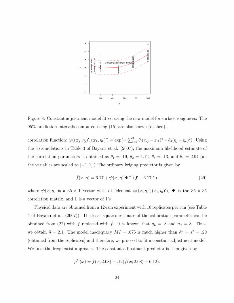
The model is plotted in Figure 8, which shows a reasonably good fit to the data (MI = .199).

We may consider fitting a functional adjustment model to obtain further improvement over

the constant adjustment model, however, in this case little would be achieved by doing that.

An Example: Spot Welding Experiment

Consider the spot welding experiment given in Higdon et al. (2004) and Bayarri et al. (2007).

There are three factors in this experiment: load (x1), current (x2), and gage (x3), and the

objective is to optimize the nugget diameter of the weld (y). The engineering model is quite

complex and contains one calibration parameter (η).

The first step is to approximate the engineering model. Because there is no random error

in the engineering model simulations, an interpolating model such as kriging is suitable for

the model approximation (Sacks et al. 1989). We fit an ordinary kriging model with Gaussian

23

20 40 60 80 100

01

23

45

6

x

y

Constant adjustment model

Figure 8: Constant adjustment model fitted using the new model for surface roughness. The

95% prediction intervals computed using (15) are also shown (dashed).

correlation function: ψ((xj, ηj)′, (xk, ηk)

′) = exp(−∑3

i=1 θi(xij − xik)2− θ4(ηj − ηk)2). Using

the 35 simulations in Table 3 of Bayarri et al. (2007), the maximum likelihood estimate of

the correlation parameters is obtained as θ1 = .19, θ2 = 1.12, θ3 = .13, and θ4 = 2.94 (all

the variables are scaled to [−1, 1].) The ordinary kriging predictor is given by

f(x; η) = 6.17 +ψ(x, η)′Ψ−1(f − 6.17 1), (29)

where ψ(x, η) is a 35 × 1 vector with ith element ψ((x, η)′, (xi, ηi)′), Ψ is the 35 × 35

correlation matrix, and 1 is a vector of 1’s.

Physical data are obtained from a 12-run experiment with 10 replicates per run (see Table

4 of Bayarri et al. (2007)). The least squares estimate of the calibration parameter can be

obtained from (22) with f replaced with f . It is known that ηL = .8 and ηU = 8. Thus,

we obtain η = 2.1. The model inadequacy MI = .675 is much higher than σ2 = s2 = .20

(obtained from the replicates) and therefore, we proceed to fit a constant adjustment model.

We take the frequentist approach. The constant adjustment predictor is then given by

µC(x) = f(x; 2.08)− .12(f(x; 2.08)− 6.12).

24

The MI = .669, which shows no significant improvement over the engineering model. There-

fore, we fit a functional adjustment model. Consider the main effects and two-factor inter-

actions of the three variables. Thus, after centering, u1 = x1, u2 = x2 − .03, u3 = x3,

u4 = x1x2, u5 = x1x3, and u6 = x2x3 − .33. We find that all the effects except u5 are

significant (|z| >√

2). Thus, we obtain the following functional adjustment model

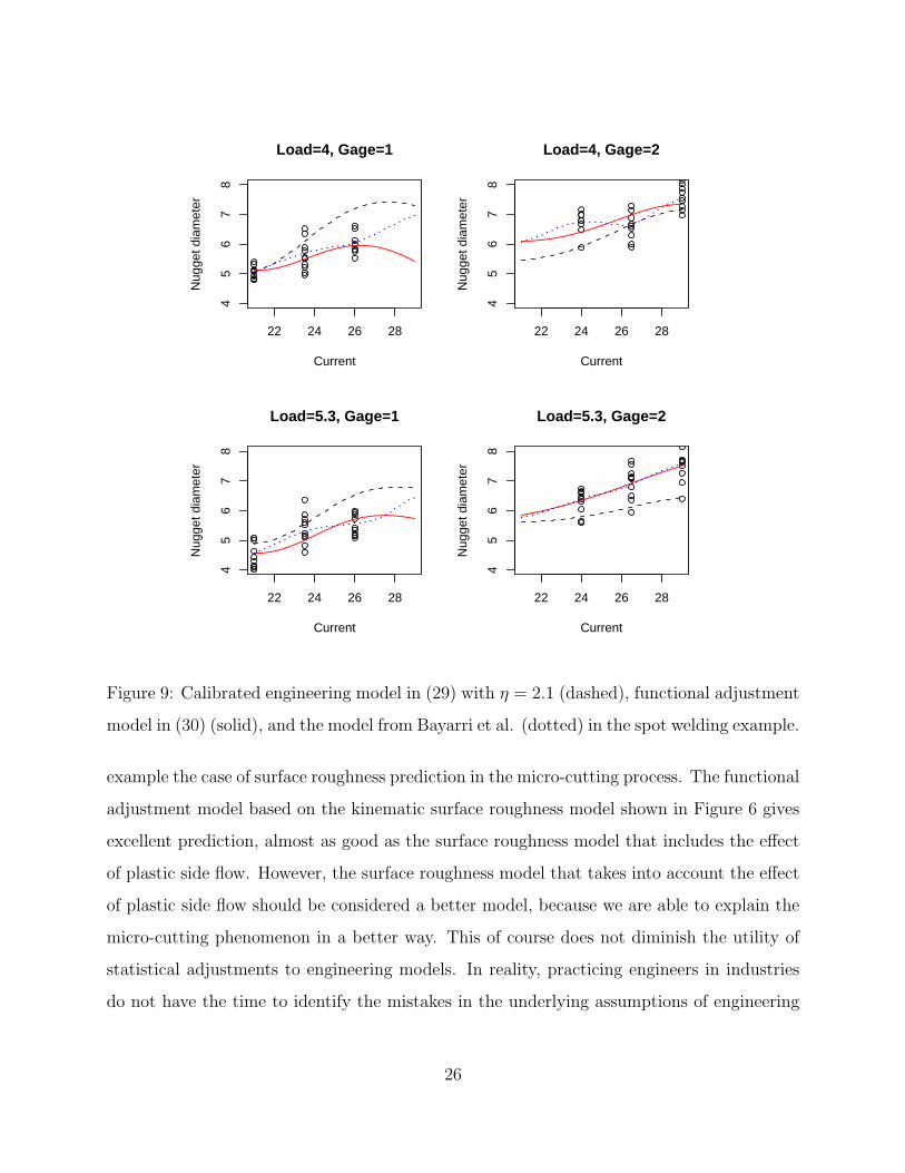
µF (x)− µC(x) = .12x1 − .21(x2 − .03) + .65x3 + .44x1x2 + .40(x2x3 − .33). (30)

The model inadequacy MI = .229 is not significant at 5% level and thus, it is a good

model for prediction. The functional adjustment model is plotted in Figure 9 for various

combinations of current, load, and gage. Clearly, the predictions are much closer to the data

than those from the calibrated engineering model (f(x; 2.1)). The model from Bayarri et al.

(2007) is also plotted in the figure (see Figure 5 in their paper). The prediction performances

of the two models near the data points are comparable, but Bayarri et al.’s model completely

changes the shape of the engineering model, which is undesirable. Whereas the proposed

model approximately preserves the shape of the engineering model and therefore, it is more

reliable and clearly better for optimizing the nugget diameter. Moreover, the fitting in

Bayarri et al. uses Markov Chain Monte Carlo methods, which are computationally much

more intensive compared to the proposed approach.

Conclusions

Engineering models and statistical models have their own pros and cons. It is shown that

through careful integration we can develop models that mitigate the drawbacks of both types

of models. Such models can help engineers develop improved process control strategies and

find better processing conditions.

The statistical adjustments correct the engineering model without trying to understand

the mistakes made in modeling the physics of the process. This is good in the sense that

we are able to quickly develop models that yield more realistic predictions. The drawback

is that we are not able to determine what went wrong in the engineering model. Take for

25

22 24 26 28

45

67

8

Load=4, Gage=1

Current

Nug

get d

iam

eter

22 24 26 28

45

67

8

Load=4, Gage=2

Current

Nug

get d

iam

eter

22 24 26 28

45

67

8

Load=5.3, Gage=1

Current

Nug

get d

iam

eter

22 24 26 28

45

67

8

Load=5.3, Gage=2

Current

Nug

get d

iam

eter

Figure 9: Calibrated engineering model in (29) with η = 2.1 (dashed), functional adjustment

model in (30) (solid), and the model from Bayarri et al. (dotted) in the spot welding example.

example the case of surface roughness prediction in the micro-cutting process. The functional

adjustment model based on the kinematic surface roughness model shown in Figure 6 gives

excellent prediction, almost as good as the surface roughness model that includes the effect

of plastic side flow. However, the surface roughness model that takes into account the effect

of plastic side flow should be considered a better model, because we are able to explain the

micro-cutting phenomenon in a better way. This of course does not diminish the utility of

statistical adjustments to engineering models. In reality, practicing engineers in industries

do not have the time to identify the mistakes in the underlying assumptions of engineering

26

models, develop new theory, and make corrections to the predictions. The engineering-

statistical models are a better alternative for them.

Although not directly evident, the engineering-statistical models may help researchers

in pin-pointing the mistakes in the assumptions and guide them in developing a better

engineering model. We leave this important topic for future research.

Appendix: Proofs

Proof of Equation (9)

Assume that the engineering model is evaluated at {x1, . . . ,xn, . . . ,xN}, which contains

the locations for the physical experiment. Therefore, β0, β1, and S are constants for given

f c = (f(x1), . . . , f(xN))′. As mentioned before, only the information from f c is used for

constructing the metamodel. Thus, let f(x) = E(f(x)|f c) and v(x) = var(f(x)|f c). Then,

E(µ(x)|y,f c) = E{E[µ(x)|y,f c, f(x)]}

= E{f(x) + β0 + β1(f(x)− f)|y,f c}

= f(x) + β0 + β1(f(x)− f),

and

var(µ(x)|y,f c) = E{var[µ(x)|y,f c, f(x)]}+ var{E[µ(x)|y,f c, f(x)]}

= E{ 1

n+ σ2/τ 20

+(f(x)− f)2

S + σ2/τ 21

|y,f c}

+var{f(x) + β0 + β1(f(x)− f)|y,f c}

=1

n+ σ2/τ 20

+(f(x)− f)2 + v(x)

S + σ2/τ 21

+ (1 + β1)2v(x).

Using a normal approximation to the distribution of µ(x) + ε|{y,f c}, we obtain the predic-

tion interval given in (9).

Proof of Equation (20)

Let β = (F ′F )−1F ′(y − f) and α = (U ′U)−1U ′(y − f − F β) be the least squares

estimates of β and α, respectively. Then, the prediction variance of a new observation is

27

given by

V = var{f(x) +w(x)′β + u(x)′α+ ε}

= var{w(x)′β + u(x)′α}+ σ2

= var{w(x)′(F ′F )−1F ′(y − f) + u(x)′(U ′U)−1U ′(y − f − F (F ′F )−1F ′(y − f))}+ σ2

= var{a(x)′(y − f)}+ σ2,

where

a(x)′ = w(x)′(F ′F )−1F ′ + u(x)′(U ′U)−1U ′(I − F (F ′F )−1F ′).

Therefore,

V = σ2a(x)′a(x) + σ2

= σ2{1 +w(x)′(F ′F )−1w(x) + u(x)′(U ′U)−1U ′(I − F (F ′F )−1F ′)U(U ′U)−1u(x)}

= σ2{1 +1

n+

(f(x)− f)2

S+ u(x)′[(U ′U)−1 −A]u(x)},

where A = (U ′U )−1U ′F (F ′F )−1F ′U(U ′U)−1. Thus, f(x) + w(x)′β + u(x)′α + ε has a

normal distribution with mean µF (x) and variance V . Therefore, the prediction interval is

given by µF (x)± zα/2√V .

Acknowledgments

This research was supported by U. S. National Science Foundation grant CMMI-0654369.

References

Bayarri, M. J.; Berger, J. O.; Paulo, R.; Sacks, J.; Cafeo, J.; Cavendish, J.; Lin, C. H.; Tu,

J. (2007). “A Framework for Validation of Computer Models”. Technometrics 49, pp.

138-154.

Box, G. E. P. and Hunter, W. G. (1962). “A Useful Method for Model-Building”. Techno-

metrics 4, pp. 301-318.

28

Breiman, L. (1995). “Better Subset Regression Using the Nonnegative Garrote”. Techno-

metrics 37, pp. 373-384.

Higdon, D.; Kennedy, M.; Cavendish, J. C.; Cafeo, J. A.; and Ryne, R. D. (2004). “Com-

bining Field Data and Computer Simulations for Calibration and Prediction”. SIAM

Journal of Scientific Computing 26, pp. 448-466.

Joseph, V. R. (2006a). “A Bayesian Approach to the Design and Analysis of Fractionated

Experiments”. Technometrics 48, pp. 219-229.

Joseph, V. R. (2006b). “Limit Kriging”. Technometrics 48, pp. 458-466.

Joseph, V. R. and Delaney, J. D. (2007). “Functionally Induced Priors for the Analysis of

Experiments”. Technometrics 49, pp. 1-11.

Joseph, V. R. and Delaney, J. D. (2008). “Analysis of Optimization Experiments”. Journal

of Quality Technology 40, pp. 282-298.

Kapoor, S. G.; DeVor, R. E.; Zhu, R.; Gajjela, R.; Parakkal, G.; and Smithey, D. (1998).

“Development of Mechanistic Models for the Prediction of Machining Performance:

Model Building Methodology”. Machining Science and Technology 2, pp. 213-238.

Kennedy, M. C. and O’Hagan, A. (2001). “Bayesian Calibration of Computer Models”

(with discussion). Journal of Royal Statistical Society - Series B 63, pp. 425-464.

Liu, K. and Melkote, S. N. (2006). “Effect of Plastic Side Flow on Surface Roughness in

Micro-Turning Process”. International Journal of Machine Tools and Manufacture 46,

pp. 1778-1785.

Loeppky, J. L.; Bingham, D.; and Welch, W. J. (2006). “Computer Model Calibration

or Tuning in Practice”. Technical Report 221, Department of Statistics, University of

British Columbia, Canada.

Marusich, T. D. and Ortiz, M. (1995). “Modeling and Simulation of High-Speed Machin-

ing”. International Journal for Numerical Methods in Engineering 38, pp. 3675-3694.

29

Neter, J.; Kutner, M. H.; Nachtsheim, C. J.; and Wasserman, W. (1996). Applied Linear

Statistical Models. McGraw-Hill, Boston, MA.

Oxley, P. L. B. (1989). Mechanics of Machining. Ellis Harwood Ltd., Chichester.

Qian, P. and Wu, C. F. J. (2008). “Bayesian Hierarchical Modeling for Integrating Low-

Accuracy and High-Accuracy Experiments”. Technometrics 50, pp. 192-204.

Reese, C. S.; Wilson, A. G.; Hamada, M.; Martz, H. F.; and Ryan, K. J. (2004). “Integrated

Analysis of Computer and Physical Experiments”. Technometrics 46, pp. 153-164.

Sacks, J.; Welch, W. J.; Mitchell, T. J.; and Wynn, H. P. (1989). “Design and Analysis of

Computer Experiments”. Statistical Science 4, pp. 409-423.

Santner, T. J.; Williams, B. J.; and Notz, W. I. (2003). The Design and Analysis of

Computer Experiments. Springer, New York, NY.

Shaw, M. C. (1997). Metal Cutting Principles. Oxford University Press, London.

Tibshirani, R. (1996). “Regression Shrinkage and Selection via the LASSO”. Journal of the

Royal Statistical Society, Ser. B 58, pp. 267-288.

Wu, C. F. J. and Hamada, M. (2000), Experiments: Planning, Analysis, and Parameter

Design Optimization, Wiley, New York, NY.

30