Embed Size (px)
Citation preview

Statistical Analysis of Compositional Data
Statistical Analysis of
Compositional Data
Carles Barcelo Vidal
J. Antoni Martın Fernandez
Santiago Thio Fdez-Henestrosa
Dept. d’Informatica i Matematica Aplicada
Universitat de Girona
Campus de Montilivi
E-17071 Girona
Catalunya – Spain.

Statistical Analysis of Compositional Data 2
What is compositional data?
Traditionally,
Composition
| |positive vector x = (x1, . . . , xD)′
whose components are subject to
a constant sum restriction:
x1 + . . . + xD = constant.
Compositional data ≡ Closed data

Statistical Analysis of Compositional Data 3
What is compositional data?
A positive vector w = (w1, . . . , wD)′
is compositional when our interest
lies on the relative magnitudes wj/wk of
its parts and not on the absolute values
Scale-invariance property
If a positive vector w = (w1, . . . , wD)′ is
compositional, the vectors w and kw,
with k > 0, give us the same information

Statistical Analysis of Compositional Data 4
USA - President election - 2000
States Bush Gore Others Total
Alabama 943799 696741 26270 1666810
Alaska 136068 64252 30347 230667
......
......
...
Wisconsin 1235035 1240431 114415 2589881
Wyoming 147674 60421 5331 213426
Alabama 56,6% 41,8% 1,6% 100%
Alaska 59,0% 27,9% 13,1% 100%
..
....
..
.... 100%
Wisconsin 47,7% 47,9% 4,4% 100%
Wyoming 69,2% 28,3% 2,5% 100%

Statistical Analysis of Compositional Data 5
Activity patterns of a statistician
Daily time (hours) devoted by an academic statistician to
different activities: te = teaching; co = consultation; ad
= administration; re = research; ot = other wakeful
activities; sl = sleep.
D te co ad re ot sl Total
1 3,5 2,0 4,5 2,5 6,5 5,0 24
2 4,0 2,0 2,5 3,0 6,5 6,0 24
.
.
.
.
.
.
.
.
.
.
.
.
.
.
.
.
.
.
.
.
.
.
.
.
19 2,5 2,5 3,0 2,0 5,0 8,5 24
20 2,5 2,0 3,0 3,0 4,0 9,0 24
1 14,4% 8,3% 18,8% 10,4% 27,1% 20,8% 100%
2 16,7% 8,3% 10,4% 2,5% 27,1% 25,0% 100%
.
.
.
.
.
.
.
.
.
.
.
.
.
.
.
.
.
.
.
.
. 100%
19 10,4% 10,4% 12,5% 8,3% 20,8% 35,4% 100%
20 10,5% 8,3% 12,5% 12,5% 16,7% 37,5% 100%

Statistical Analysis of Compositional Data 6
Artic lake
Sand, silt, clay composition (% by weight) of 39sediment samples from an Artic lake
Sample Sand Silt Clay Total
S01 77.5 19.5 3.0 100%
S02 71.9 24.9 3.2 100%
.
.....
.
..... 100%
S39 2.0 47.8 50.2 100%

Statistical Analysis of Compositional Data 7
Volcano H
Percentage of Cl, K2O, P2O5, TiO2 and SiO2 in46 samples of volcanic rocks from a volcano H
Sample Cl K2O P2O5 TiO2 SiO2 Total
1 0.0638 1.83 1.01 3.70 44.99 51.59%
2 0.1116 1.36 0.81 3.83 43.45 49.56%
3 0.0611 1.36 1.09 4.10 42.98 49.59%
.
.
.
.
.
.
.
.
.
.
.
.
.
.
.
.
.
.
.
.
.
44 0.0477 1.67 0.96 3.64 45.14 51.46%
45 0.0015 1.70 0.95 3.64 45.15 51.44%
46 0.0986 3.22 0.50 1.87 54.41 60.10%

Statistical Analysis of Compositional Data 8
Halimba boreholes
Percentages of Al2O3, SiO2, Fe2O3, TiO2, H2OCaO and MgO in some samples from differentdrills in Halimba region (Hungary)
Al2O3 SiO2 Fe2O3 TiO2 H2O CaO MgO Total
52,5 6,7 23,6 2,6 12,0 0,2 0,1 97,7%
47,7 4,6 32,1 2,3 12,0 2,0 0,0 100,7%
50,6 8,9 25,4 2,5 11,9 1,1 0,0 100,4%
.
.
.
.
.
.
.
.
.
.
.
.
.
.
.
.
.
.
.
.
.
.
.
.

Statistical Analysis of Compositional Data 9
The space of compositions
Any D × 1 real vector w = (w1, . . . , wD)′ withpositive components w1, . . . , wD will be called aD-observational vector.
Therefore, the set of these vectors will be IRD+ , the
positive orthant of IRD.
Definition Two D-observational vectors w andw∗ are compositionally equivalent, w ∼ w∗, whenthere exists a positive proportionality constant k
such that w = kw∗.
This relation classifies the vectors of IRD+ in
classes of equivalence, called D-compositions.
The composition generated by an observationalvector w will be symbolized by w, i.e.,
w = {kw : k ∈ IR+}.

Statistical Analysis of Compositional Data 10
Scale invariance
Definition A function f defined on IRD+ is said
to be scale invariant if
f(kw) = f(w) for every w ∈ IRD+ and k ∈ IR+
or equivalently
f(w) = f(w∗) when w ∼ w∗.
Property Any scale invariant function f(w)defined on IRD
+ can be expressed in terms of ratiosof the components w1, . . . , wD of w, such as
w1/wD, . . . wD−1/wD or w1/g(w), . . . , wD/g(w),
where g(w) = (w1w2 . . . wD)1/D is the geometricmean of the components of w.
Property Any function defined on thecompositional space CD−1 arises from a scaleinvariant function defined on the positive realspace IRD
+ .
Statistical Analysis of Compositional Data 11
The space of compositions
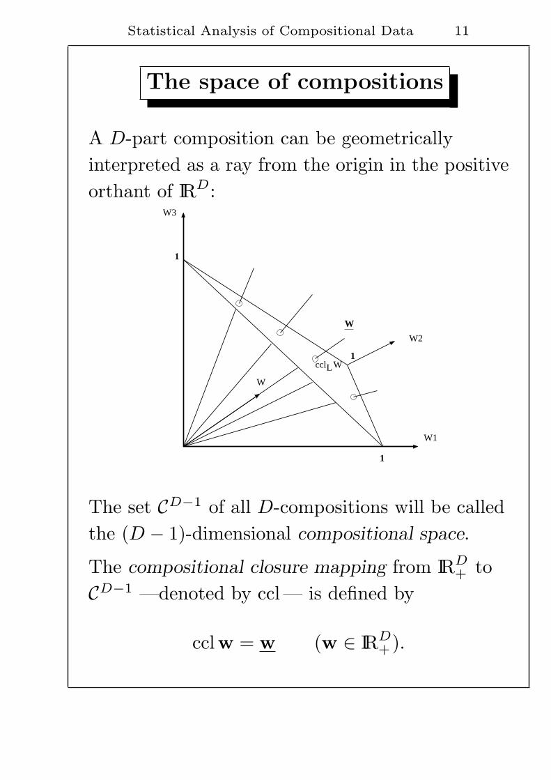
A D-part composition can be geometricallyinterpreted as a ray from the origin in the positiveorthant of IRD:
W3
W2
W1
Lccl W
W
W
1
1
1
The set CD−1 of all D-compositions will be calledthe (D − 1)-dimensional compositional space.
The compositional closure mapping from IRD+ to
CD−1 —denoted by ccl — is defined by
cclw = w (w ∈ IRD+).

Statistical Analysis of Compositional Data 12
Representation of a composition
Linear criterion
Definition The linear criterion selects fromeach D-composition w the D-observational vectorw∗ —with components w∗1 , . . . , w∗D— whose sumis equal to 1. If this vector is symbolized bycclL w —or by Cw— then
cclL w = Cw = w/D∑
j=1
wj (w ∈ IRD+).
The set of all the vectors x = cclL w (w ∈ IRD+) is
the well-known (D − 1)-dimensional simplex SD.

Statistical Analysis of Compositional Data 13
Linear criterion
W3
W2
W1
Lccl W
W
W
1
1
1
1
2 3
x2
x3
x1

Statistical Analysis of Compositional Data 14
Representation of a composition
Other criteria
Spherical criterionW3
W2
W1
W
E
1
1
1ccl W
W
Hyperbolic criterion
1
W2
1 W1
W
Hccl W
W

Statistical Analysis of Compositional Data 15
Subcompositions
Sometimes, given a composition w in CD−1, wemay wish to focus attention on the relativemagnitudes of a subset of components.
Definition If S is any subset of the indices1, . . . , D of a given a D-composition w ∈ CD−1,and wS is the subvector formed from thecorresponding components of w, thenwS = cclwS is termed a subcomposition.
If the subset S is formed by C indices, with2 ≤ C < D, the subcomposition wS belongs tothe compositional space CC−1.
Definition The formation of a C-subcompo-sition wS from a D-composition w may beconsidered as the mapping subS from CD−1 toCC−1:
subS w = wS (w ∈ CD−1)

Statistical Analysis of Compositional Data 16
Subcompositions
W3
W2
W1
W
W
1
1
1
W12
W 12
Lccl W
1
2 3
L 12ccl W
Lccl W

Statistical Analysis of Compositional Data 17
Compositional Problems
1. Percentage of Cl, K2O, P2O5, TiO2 and SiO2
in 46 samples of volcanic rocks from a volcanoH:
Num. Cl K2O P2O5 TiO2 SiO2
1 0.0638 1.83 1.01 3.70 44.99
2 0.1116 1.36 0.81 3.83 43.45
3 0.0611 1.36 1.09 4.10 42.98
......
......
......
44 0.0477 1.67 0.96 3.64 45.14
45 0.0015 1.70 0.95 3.64 45.15
46 0.0986 3.22 0.50 1.87 54.41
Statistical Analysis of Compositional Data 18
Compositional Problems
1.a It is possible to describe the pattern ofvariability of these volcanic rocks and todefine a covariance or correlation structure?
1.b Is it possible to define a measure of totalvariability of this set of volcanic rocks?
1.c For a new volcanic rock specimen with knowncomposition (Cl,K2O,P2O5,TiO2,SiO2)’ andclaimed to be from the same volcano, can wesay whether it is fairly typical from thisvolcano? If not, can we place some measureon its atypicality?
1.d To what extent, if any, do the subcomposition(Cl,K2O,P2O5) explain the pattern ofvariability of the full composition?

Statistical Analysis of Compositional Data 19
Compositional Problems
1.e From this ternary diagram it seems that thepattern of (K2O,P2O5,TiO2) can be welladjusted by a curve. How can we confirmthis?

Statistical Analysis of Compositional Data 20
Compositional Problems
2. Percentage of Cl, K2O, P2O5, TiO2 and SiO2:65 samples of volcanic rocks from a volcanoA, and 19 samples from another volcano D.
Num. Cl K2O P2O5 TiO2 SiO2
1A 0.1776 0.64 0.34 1.57 49.26
2A 0.2050 1.55 0.43 1.61 48.22
.
.....
.
.....
.
.....
65A 0.0391 1.70 0.55 1.63 50.91
1D 0.0181 0.64 0.31 2.55 49.33
2D 0.0053 1.10 0.59 2.81 46.89
.
.....
.
.....
.
.....
19D 0.0200 0.99 0.37 3.16 45.85

Statistical Analysis of Compositional Data 21
Compositional Problems
2.a Can we detect any differences between thecompositional pattern of volcano A andvolcano D?
If so, how can we choose a 3-partsubcomposition which somehow captures theessence of the two patterns individually andyet emphasizes the differences between thepatterns?
2.b Is it possible to establish a classification rulefor discriminating between volcanos A and D?

Statistical Analysis of Compositional Data 22
Compositional Problems
3. Sand, silt,clay composition (% by weight) of39 sediment samples at different water depthsin an Artic lake:
Num. Sand Silt Clay Depth (m)
S01 77.5 19.5 3.0 10.4
S02 71.9 24.9 3.2 11.7
.
.....
.
.....
.
..
S39 2.0 47.8 50.2 103.7
3.a Is sediment composition dependent onwater depth?
3.b If so, how can we quantify the extent ofthe dependence?

Statistical Analysis of Compositional Data 23
How to analyze ”closed” raw data?
Spurious correlations
Pearson (1897) ”If u = f(x, y) andv = g(z, y) be two functions of three variablesx, y, z, and these variables be selected at randomso that there exists no correlation between x andy, y and z, or z and x, there will still be found toexist correlation between u and v. . . . That islikely to occur when u and v are indices with thesame denominator”.
Consequence The standard covariance matrix[sij ] of a closed data set from SD is alwayssingular because
D∑
j=1
sij = 0, for i = 1, . . . , D.

Statistical Analysis of Compositional Data 24
How to analyze ”closed” raw data?
Subcompositional incoherence
Example
Scientist A Scientist B
Full compositions from S4 Subcompositions from S3
(x1, x2, x3, x4) (s1, s2, s3)
(0.1, 0.2, 0.1, 0.6) (0.250, 0.500, 0.250)
(0.2, 0.1, 0.1, 0.6) (0.500, 0.250, 0.250)
(0.3, 0.3, 0.2, 0.2) (0.375, 0.375, 0.250)
corr{x(1),x(2)} = 0.5 corr{s(1), s(2)} = −1
Any statement that scientists A and B makeabout the common parts 1,2 and 3 must agree.

Statistical Analysis of Compositional Data 25
Statistics in IRD
Translation In IRD the inner operation istranslation. If t ∈ IRD, the translation t movesthe random vector X in IRD to a random vectorX + t in such a way that
E{X + t} = E{X}+ t and Σ{X + t} = Σ{X}.
Scalar product For any random vector X onIRD and for any λ ∈ R,
E{λX} = λE{X} and Σ{λX} = λ2Σ{X}.

Statistical Analysis of Compositional Data 26
Perturbations on CD−1
Scale invariance is the property which characteri-zes compositional data. Therefore, any ”opera-tion” involving compositions must be compatiblewith this property.
Definition We define an inner operation ⊕ inCD−1 as
w ⊕w∗ = ccl (w1w∗1 , . . . , wDw∗D)′.
(CD−1,⊕) is a commutative group:
• Composition 1D = ccl (1, . . . , 1)′ is theneutral element.
• The inverse composition w−1 ofw = ccl (w1, . . . , wD)′ is the compositionw−1 = ccl (1/w1, . . . , 1/wD)′.

Statistical Analysis of Compositional Data 27
The group of perturbations in CD−1
Definition Given a composition p ∈ CD−1, theperturbation associated to p is the transformationfrom CD−1 to CD−1 defined by
c → p⊕ c (c ∈ CD−1).
Then, we say that p⊕ c is the composition whichresults when the perturbation p is applied to thecomposition c.
Moreover, given two compositions of CD−1
w = ccl (w1, . . . , wD)′, w∗ = ccl (w∗1 , . . . , w∗D)′,
there exists a unique perturbation p which trans-forms w on w∗:
p = w∗ ⊕w−1 = ccl(
w∗1w1
, . . . ,w∗DwD
)′.

Statistical Analysis of Compositional Data 28
The group of perturbations in CD−1
X1
X2 X3
X1
X2 X3
e
x
pox
p
X1
X2 X3
x
x*
xox* −1

Statistical Analysis of Compositional Data 29
The group of perturbations in CD−1
Perturbation in compositional space plays thesame role as translation plays in real space. Theset of all perturbations in CD−1 is a commutativegroup isomorphic to (CD−1,⊕). For this reason,we will also call perturbation the inner operation⊕ defined on CD−1.
The assumption that the group of perturbationsis the operating group on the compositional spaceis the keystone of the methodology introduced byAitchison (1986). In fact, it implies to accept thatthe “difference” between two compositionsw = ccl (w1, . . . , wD)′ and w∗ = ccl (w∗1 , . . . , w∗D)′
will be based on the ratios w∗j /wj between partsinstead of on the arithmetic differences w∗j − wj .

Statistical Analysis of Compositional Data 30
Perturbations on CD−1
Interpretation
• Some natural processes in nature can beinterpreted as a succession of changes fromone initial composition w0 to a finalcomposition wn through the application ofsuccessive perturbations:
w0 −→ p1 ⊕w0 = w1
−→ p2 ⊕w1 = w2
. . .
−→ pn ⊕wn−1 = wn.
In this manner,
wn = (pn ⊕ pn−1 ⊕ . . .p1)⊕w0.

Statistical Analysis of Compositional Data 31
Genesis of normal distribution
Particles fall from a funnel onto tips of triangles, where
they are deviated to the left or to the right with equal
probability (0.5) and finally fall into receptacles. If the tip
of a triangle is at distance x from the left edge of the
board, triangle tips to the right and to the left below it are
placed at x + k and x− k (k constant).

Statistical Analysis of Compositional Data 32
Genesis of lognormal distribution
Particles fall from a funnel onto tips of triangles, where
they are deviated to the left or to the right with equal
probability (0.5) and finally fall into receptacles. If the tip
of a triangle is at distance x from the left edge of the
board, triangle tips to the right and to the left below it are
placed at x/k and x.k (k constant).

Statistical Analysis of Compositional Data 33
Perturbations on CD−1
Interpretation
• If w = ccl (wSiO2 , . . . , wP2O5)′ expresses the
percentage composition of major oxides of arock, its molecular composition will be
w∗ = ccl (wSiO2/mSiO2 , . . . , wP2O5/mP2O5)′,
where mj symbolizes the molecular weight ofoxide j.
Therefore, composition w∗ can be obtainedapplying the perturbation
m−1 = (ccl (mSiO2 , . . . , mP2O5)′)−1
to composition w:
w∗ = m−1 ⊕w.

Statistical Analysis of Compositional Data 34
The vector space (CD−1,⊕,⊗)
Definition The external operation ⊗ in CD−1 isdefined as
λ⊗w = ccl (wλ1 , . . . , wλ
D)′,
for each λ ∈ IR and each w ∈ CD−1.
(CD−1,⊕,⊗) is a vector space of dimension D− 1.
X1
X2 X3
X1
X2 X3
X1
X2 X3
X1
X2 X3
X1
X2 X3
e
x
2.x
−2.x

Statistical Analysis of Compositional Data 35
The log and the exp transformations
between IRD+ and IRD
The logarithmic transformation on IRD+ trans-
forms the rays from the origin —which representthe compositions of the space CD−1—, to straightlines of IRD parallel to vector 1D = (1,
D. . ., 1)′.
Inversely, the exponential transformation on IRD
transforms these straight lines of IRD parallel tovector 1D, to rays from the origin of IRD
+ .

Statistical Analysis of Compositional Data 36
W2
W1
W
W
ccl W
1
1
U
z+U
Z2
Z1
z
ucl z V
1
1

Statistical Analysis of Compositional Data 37
Centered logratio transformation
Definition The centered logratio transforma-
tion —denoted by clr — is the one-to-one functionfrom the compositional space CD−1 to thesubspaceV = {z = (z1, . . . , zD)′ ∈ IRD : z1 + . . . + zD = 0}of IRD, defined by
clrw = logw
g(w)(w ∈ CD−1).
The inverse transformation, from V to CD−1, isgiven by
clr−1 z = ccl (exp z) (z ∈ V ).
The logarithmic and the exponential transforma-tions establish a one-to-one correspondencebetween the simplex SD and the hyperplan V inIRD.

Statistical Analysis of Compositional Data 38
Centered logratio transformation
W2
W1
W
W
ccl W
1
1
U
z+U
Z2
Z1
z
ucl z V
1
1

Statistical Analysis of Compositional Data 39
Centered logratio transformation
Property The centered logratio transforma-
tion is an isomorphism between the vector space(CD−1,⊕,⊗) and the vector subspace
V = {z = (z1, . . . , zD)′ ∈ IRD : z1 + . . . + zD = 0}
of (IRD, +, .). Therefore,
clr (w ⊕w∗) = clrw + clrw∗ ;
clr (λ⊗w) = λ clrw,
where w,w∗ ∈ CD−1, and λ ∈ <.
Equally,
clr−1 (z + z∗) = clr−1 z⊕ clr−1 z∗ ;
clr−1 (λ z) = λ⊗ clr−1 z,
where z, z∗ ∈ V , and λ ∈ IR.

Statistical Analysis of Compositional Data 40
Isometric logratio transformation
Let V = {v1, . . . ,vD−1} an orthonormal basis ofthe subspace
V = {z = (z1, . . . , zD)′ ∈ IRD : z1 + . . . + zD = 0}.Then, since clrw ∈ V , it will be always possibleto write
clrw = u1v1 + . . . + uD−1vD−1,
for any w ∈ CD−1.
Definition The isometric logratio
transformation —denoted by ilrV — is theone-to-one function from the compositional spaceCD−1 to IRD−1 defined by
ilrV w = (u1, . . . , uD−1)′ (w ∈ CD−1).
Like clr , the transformation ilrV is anisomorphism between the vector spaces(CD−1,⊕,⊗) and (IRD−1,+, .).

Statistical Analysis of Compositional Data 41
Skye Lavas
Sample Na2O + K2O Fe2O3 MgO
S1 52 42 6
S2 52 44 4
S3 47 48 5
clr (Na2O + K2O) clr (Fe2O3) clr (MgO)
S1 0,7910 0,5775 -1,3685
S2 0,9107 0,7436 -1,6543
S3 0,7399 0,7609 -1,5008
ilr 1 [u1] ilr 2 [u2]
S1 0,1510 1,6760
S2 0,1181 2,0261
S3 -0,0149 1,8381
Hint The orthonormal basis V of the subspace V ⊂ IR3
linked to the ilr coordinates is
v1 = (1√2
,− 1√2
, 0)′, v2 = (1√6
,1√6
,− 2√6)′

Statistical Analysis of Compositional Data 42
Skye Lavas
Ternary diagram
clr-coordinates ilr-coordinates

Statistical Analysis of Compositional Data 43
CD−1 as an Euclidean space
The clr transformation between CD−1 and thesubspace V of IRD allows to translate to CD−1 thereal Euclidean structure defined on V :
<w,w∗>C = (clrw)′ clrw∗
= (log w)′HD log w∗,
‖w‖C = ‖clrw‖= [(log w)′HD log w]1/2,
d C(w,w∗) = d Euc(clrw, clrw∗)
= [(log w∗ − log w)′HD
(log w∗ − log w)]1/2,
where HD is the (D ×D)-centering matrix. Thismatrix is equal ID −D−1JD, where ID is theidentity matrix and JD = 1D1′D.
Therefore, by construction, transformations clrand clr−1 —and also ilr and ilr−1— preservethe distances defined in CD−1 and IRD−1.

Statistical Analysis of Compositional Data 44
Compositional geometry in CD−1
• We can not analyze the simplex SD as weanalyze the Euclidean real space.
Let
w1 = ccl (1.000, 49.500, 39.500)′
w2 = ccl (0.010, 49.995, 39.995)′
w3 = ccl (25.0, 50.0, 25.0)′
w4 = ccl (35.0, 30.0, 35.0)′
be four compositions from S3.
Then,
d Euc(w1,w2) ≈ 1.21 < 24.49 ≈ d Euc(w3,w4),
whereas
d C(w1,w2) ≈ 3.77 > 0.69 ≈ d C(w3,w4).

Statistical Analysis of Compositional Data 45
Compositional geometry in CD−1
• Any linear variety on CD−1 —straight lines,planes, etc— can always be implicitlyexpressed by a system of linear equations inlog w1, . . . , log wD in the form
a11 log w1+ . . . +a1D log wD = b1
. . . . . . . . .
am1 log w1+ . . . +amD log wD = bm
,
with ai1 + . . . + aiD = 0, for each i = 1, . . . , m.
• In particular, the parametric equation—varying t ∈ IR— of a straight line on CD−1
is given by
w(t) = ccl (exp(α1+λ1t), . . . , exp(αD+λDt))′,
where∑D
j=1 alphaj = 0 and∑D
j=1 λj = 0.
• Similarly to real space, the concepts ofparallelism and orthogonality can beintroduced in CD−1.

Statistical Analysis of Compositional Data 46
Parallelism in C2
1
2 3
k>0 k=0 k<0
log w2 − log w3 = k
1
2 3
k=−4
k=−2
k=0
k=2
k=4
log w1 − 2 log w2 + log w3 = k

Statistical Analysis of Compositional Data 47
Orthogonality in C2
1
2
3
w2 − w3 = 0
−2 log w1 + log w2 + log w3 = 0
1
2 3
log w1 − 3 log w2 + 2 log w3 = 0
5 log w1 − log w2 − 4 log w3 = 0

Statistical Analysis of Compositional Data 48
Circles in C2
Simplex S3
−0.5 0 0.5 1 1.5 2
−1.5
−1
−0.5
0
0.5
clr -space

Statistical Analysis of Compositional Data 49
The alr transformation
Definition The additive logratio transforma-
tion of index j (j = 1, . . . , D) — denoted byalrj — is the one-to-one transformation fromCD−1 to IRD−1 defined by
w −→ y = alrj w = logw−j
wj.
where
w−j = (w1, w2, . . . , wj−1, wj+1, . . . , wD)′.
The inverse transformation of alrD , from IRD−1
to CD−1, is given by
alr−1D y = ccl (exp y1, . . . , exp yD−1, 1)′ (y ∈ IRD−1).

Statistical Analysis of Compositional Data 50
The alr transformation
Property The alrj transformations(j = 1, . . . , D) are isomorphisms between thevector spaces (CD−1,⊕,⊗) and (IRD−1,+, .), i.e.,
alrj (w ⊕w∗) = alrj w + alrj w∗ ;
alrj (λ⊗w) = λ alrj w,
alr−1j (y + y∗) = alr−1
j y ⊕ alr−1j y∗ ;
alr−1j (λ y) = λ⊗ alr−1
j y,
where w,w∗ ∈ CD−1, y,y∗ ∈ IRD−1 and λ ∈ IR.
Property The alrj transformations(j = 1, . . . , D) do not preserve the distancesdefined in the metric spaces CD−1 and IRD−1, i.e.,
d C(w,w∗) 6= d Euc(alrj w, alrj w∗);
d Euc(y,y∗) 6= d C(alr−1j y, alr−1
j y∗).

Statistical Analysis of Compositional Data 51
Determination of a composition
A composition w ∈ CD−1 can be determined inseveral forms:
(i) Giving any D-observational vector belongingto w. Usually, we will choose the vectorx = Cw = cclL w belonging to SD.
(ii) Giving the components (z1, . . . , zD)′ = z ofthe centered logratio transformed vectorclrw. Since z belongs to the subspace V ofIRD, its components are related by theequality z1 + . . . + zD = 0.
(iii) Giving the components (y1, . . . , yD−1)′ = y ofthe additive logratio transformed vectoralrD w. If it is needed, we can choose thecomponents of any other logratio alrjw(j 6= D).
(iv) Giving the components (u1, . . . , uD−1)′ = u ofthe isometric logratio transformed vectorilrV w, where V is a known orthonormal basisof the subspace V of IRD.

Statistical Analysis of Compositional Data 52
Determination of a composition
• Skye lavas: A = Na2O + K2O, F = Fe2O3, M = MgO
Sample A F M
S1 52 42 6
S2 52 44 4
clr (A) clr (F) clr (M)
S1 0.7910 0.5775 -1.3685
S2 0.9107 0.7436 -1.6543
ilr 1 [u1] ilr 2 [u2]
S1 0,1510 1,6760
S2 0,1181 2,0261
alrMA alrMF
S1 2.159 1.946
S2 2.565 2.398
alrAF alrAM
S1 -0.214 -2.159
S2 -0.167 -2.565
Hint The orthonormal basis V of the subspace V ⊂ IR3
linked to the ilr coordinates is
v1 = (1√2
,− 1√2
, 0)′, v2 = (1√6
,1√6
,− 2√6)′.

Statistical Analysis of Compositional Data 53

Statistical Analysis of Compositional Data 54
Compositional data set
• Raw data matrix
W = [wij : i = 1, . . . , n; j = 1, . . . , D],
or
X = [xij : i = 1, . . . , n; j = 1, . . . , D],
where xi = (xi1, . . . , xiD)′ ∈ SD.
Example AFM composition of 23 aphyric Skyelavas [A = Na2O + K2O, F = Fe2O3, M = MgO].
Obs. A% F% M%
S1 52 42 6
..
....
..
....
S23 24 56 20
X =
52 42 6...
......
24 56 20
.

Statistical Analysis of Compositional Data 55
Compositional data set
• Centred logratio (clr ) data matrix
Z = [zij : i = 1, . . . , n; j = 1, . . . , D],
where zij = log (wij/g(wi)), withg(wi) = (
∏Dk=1 wik)1/D.
Example AFM composition of 23 aphyric Skyelavas [A = Na2O + K2O, F = Fe2O3, M = MgO].
Obs. A% F% M%
S1 52 42 6
..
....
..
....
S23 24 56 20
clr A clr F clr M
Z =
0.791 0.577 −1.368...
......
−0.222 0.626 −0.404
.
Statistical Analysis of Compositional Data 56
Compositional data set
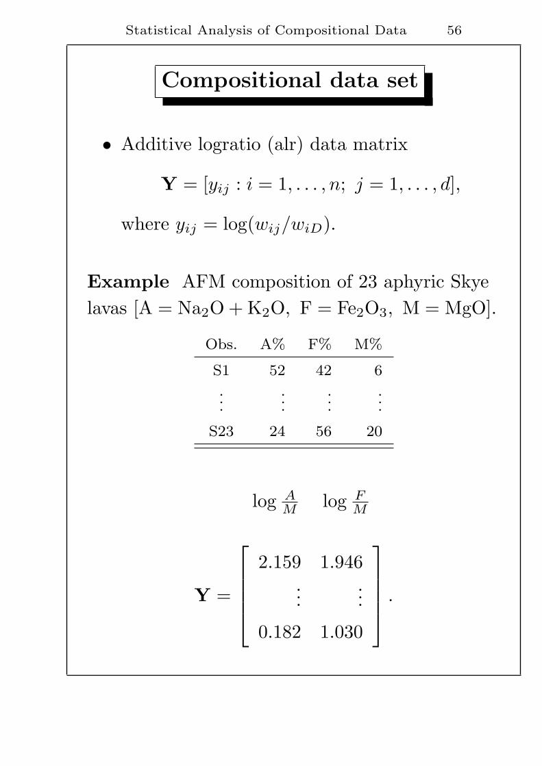
• Additive logratio (alr) data matrix
Y = [yij : i = 1, . . . , n; j = 1, . . . , d],
where yij = log(wij/wiD).
Example AFM composition of 23 aphyric Skyelavas [A = Na2O + K2O, F = Fe2O3, M = MgO].
Obs. A% F% M%
S1 52 42 6
.
.....
.
.....
S23 24 56 20
log AM log F
M
Y =
2.159 1.946...
...
0.182 1.030
.

Statistical Analysis of Compositional Data 57
Center of a compositional data set
• The center of a set W of n compositions w1,
. . . ,wn of CD−1, is the composition g definedby
cenW = g = (1n⊗w1)⊕ . . .⊕ (
1n⊗wn).
This center is equal to
g = ccl
(n∏
i=1
wi1
)1/n
, . . . ,
(n∏
i=1
wiD
)1/n′
.
• It verifies that
clrg = z =n∑
i=1
1nzi =
n∑
i=1
1n
clrwi.
and
alrD g = y =n∑
i=1
1nyi =
n∑
i=1
1n
alrD wi.

Statistical Analysis of Compositional Data 58
Center of a compositional data set
Properties
cenW = ccl
(n∏
i=1
wi1
)1/n
, . . . ,
(n∏
i=1
wiD
)1/n′
.
• cenW = argmin︸ ︷︷ ︸ξ∈CD−1
{dC(w1,ξ)+...+dC(wn,ξ)
n
}.
• cen {p⊕W} = p⊕ cenW, where p ∈ CD−1.
• cen {t⊗W} = t⊗ cenW, where t ∈ IR.
• cen {W ⊕W∗} = cenW ⊕ cenW∗.

Statistical Analysis of Compositional Data 59
Center of a compositional data set
Example AFM composition of 23 aphyric Skyelavas
? Compositional (”geometric”) center:
g = ccl (25.85, 56.65, 17.50)′.
? ”Arithmetic” center:
a = ccl (26.83, 53.74, 19.43)′.

Statistical Analysis of Compositional Data 60
Centering
To ”centre” a compositional data set w1, . . .wn
with centre g, it suffices to consider the new dataset w∗
1 = g−1 ⊕w1, . . . ,w∗n = g−1 ⊕wn.
Obviously, the centre of the new ”centered” dataset w∗
1, . . . ,w∗n is ccl (1/D, . . . , 1/D)′.

Statistical Analysis of Compositional Data 61
Compositional covariance structure
• Variation matrix
T = [τjk] =[var
{log
w(j)
w(k)
}].
? τjk = 0 means a perfect relationship between w(j)
and w(k) in the sense that the ratio w(j)/w(k) is
constant.
? The larger the value of τjk the more departure
from proportionality between w(j) and w(k).
? A measure of degree of proportionality between
two parts j and k is given by
exp(−√τjk).
In this way, exp(−√τjk) = 0 means zero
propotionality, and exp(−√τjk) = 1 means
perfect propotionality.
? The variation matrix of any subcomposition is
simply obtained by picking out on T all the
logratio variances τjk associated with the parts j
and k of the subcomposition.

Statistical Analysis of Compositional Data 62
Compositional covariance structure
• Logratio covariance matrix
Σ = [σjk] =[cov
{y(j),y(k)
}]
=[cov
{log w(j)
w(D), log w(k)
w(D)
}].,
where
yj =(
logw1j
w1D, . . . , log
wnj
wnD
)′,
for j = 1, . . . , D − 1.

Statistical Analysis of Compositional Data 63
Compositional covariance structure
• Centered covariance matrix
Γ = [γjk] =[cov
{z(j), z(k)
}].
where
z(j) = (log (w1j/g(w1)) , . . . , log (wnj/g(wn)))′ ,
for j = 1, . . . , D.
Hint. Correlation corr{z(j), z(k)
}is not a
measure of a relationship between parts j andk because is subcompositionally incoherent.
• Total (relative) variability
totvarC{W} =∑n
i=11nd2
C(wi,g) = trace {Γ}
= 12D1
′DT1D = 1
D
∑i<j τij .

Statistical Analysis of Compositional Data 64
Compositional covariance structure
• The centered covariance matrix Γ =[γjk
]is singular
becauseD∑
k=1
γjk = 0 (j = 1, . . . , D).
• The relationships between the three covariance
matrices T,Σ and Γ are linear.
• The dimensionality of the covariance structure of a
compositional raw data matrix from CD−1 is equal to12D(D − 1).
• The covariance matrix T —and also Σ and Γ— is
coherent with the algebraic structure of (CD−1,⊕,⊗),
i.e.,
T{p⊕W} = T{W} and T{λ⊗W} = λ2T{W},
where W is a compositional raw data matrix from
CD−1, p ∈ CD−1 and λ ∈ IR.
Therefore,
totvar C{p⊕W} = totvarC{W};
totvarC{λ⊗W} = λ2totvarC{W}.

Statistical Analysis of Compositional Data 65
Compositional covariance structure
Example AFM composition of 23 Skye lavas
? Variation matrix
T =
0 0.251 1.144
0.251 0 0.350
1.144 0.350 0
.
? Logratio covariance matrix
ΣA =
[0.251 0.523
0.523 1.144
]ΣF =
[0.251 −0.271
−0.271 0.350
]
ΣM =
[1.144 0.622
0.622 0.350
].
? Centered covariance matrix
Γ =
0.271 0.013 −0.284
0.013 0.007 −0.020
−0.284 −0.020 0.304
.
? Total variability: totvarC = 0.582.

Statistical Analysis of Compositional Data 66
Biplots
In general, the biplot is a simultaneous represen-tation of the rows (observations) and columns(variables) of a n× p matrix X by means of arank-2 approximation.
Usually, biplot analysis starts with performingsome transformations on X, depending on thenature of the data, to obtain a transformedmatrix Z which is the one that is actuallydisplayed.

Statistical Analysis of Compositional Data 67
Biplots
• The singular value decomposition (SVD) of Zprovides a decomposition of this matrix:
Z = [u1 : . . . : ur] diag{λ1, . . . , λr} [v1 : . . . : vr]′,
where
? r is the rank of Z;
? u1, . . . ,ur are the standardizedeigenvectors of Z′;
? v1, . . . ,vr are the standardizedeigenvectors of Z;
? and λ1, . . . , λr the corresponding positiveeigenvalues in decreasing order.
• From this SVD of Z, and using only the twofirst eigenvectors, a rank-2 approximation Zis obtained:
Z = [u1 : u2] diag{λ1, λ2} [v1 : v2]′.
Statistical Analysis of Compositional Data 68
Biplots
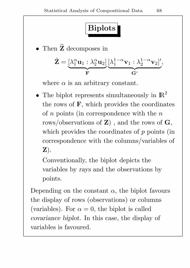
• Then Z decomposes in
Z = [λα1 u1 : λα
2 u2]︸ ︷︷ ︸F
[λ1−α1 v1 : λ1−α
2 v2]′︸ ︷︷ ︸G′
,
where α is an arbitrary constant.
• The biplot represents simultaneously in IR2
the rows of F, which provides the coordinatesof n points (in correspondence with the n
rows/observations of Z) , and the rows of G,which provides the coordinates of p points (incorrespondence with the columns/variables ofZ).
Conventionally, the biplot depicts thevariables by rays and the observations bypoints.
Depending on the constant α, the biplot favoursthe display of rows (observations) or columns(variables). For α = 0, the biplot is calledcovariance biplot. In this case, the display ofvariables is favoured.

Statistical Analysis of Compositional Data 69
Biplots
• Singular value decomposition (SVD) of Z:
Z = [u1 : . . . : ur] diag{λ1, . . . , λr} [v1 : . . . : vr]′,
• Rank-2 approximation Z:
Z = [λα1 u1 : λα
2 u2]︸ ︷︷ ︸F
[λ1−α1 v1 : λ1−α
2 v2]′︸ ︷︷ ︸G′
,
• The ratioλ1 + λ2
λ1 + . . . + λr
is a measure of the proportion of the”variability” of Z captured by the biplot.

Statistical Analysis of Compositional Data 70
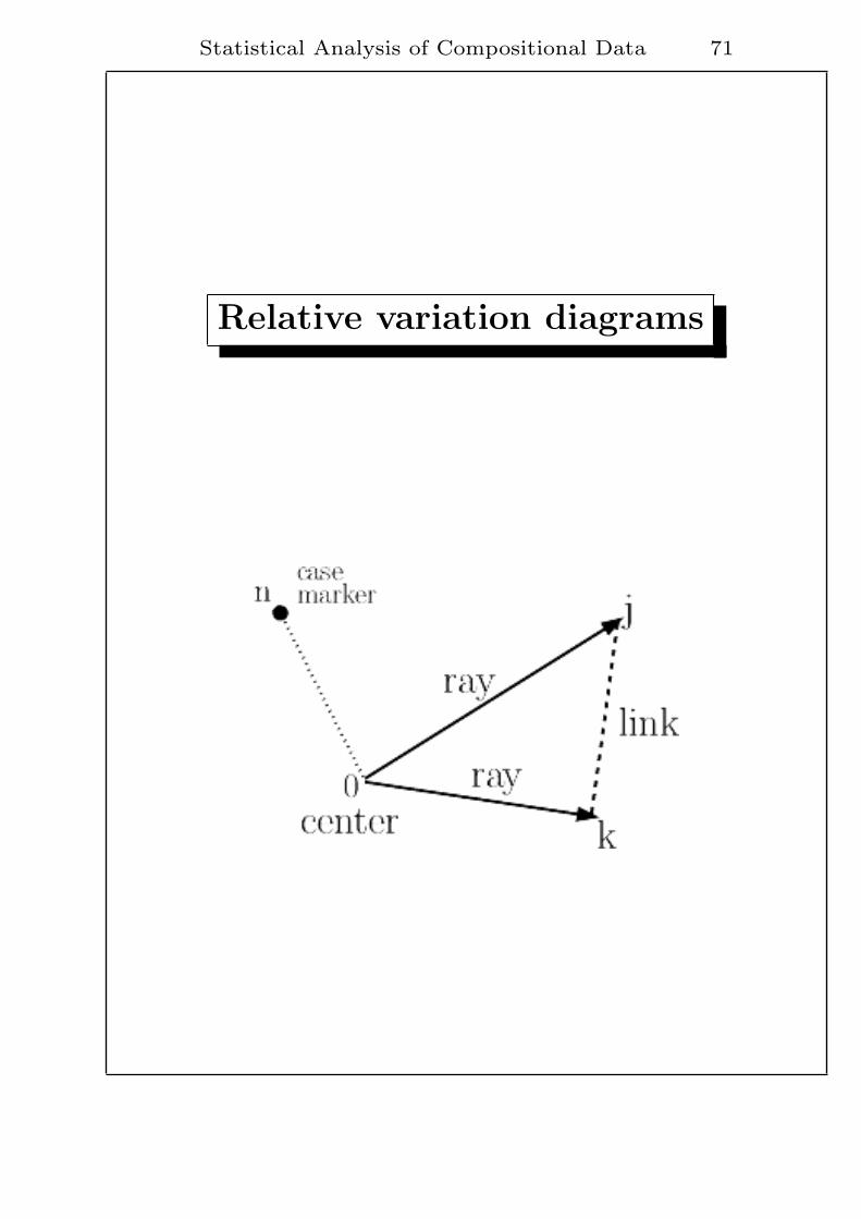
Relative variation diagrams
Definition The relative variation diagram of acompositional data set w1, . . . ,wn of CD−1 is thecovariance biplot of the matrix Zc which weobtain after centering the D columns of thecentered logratio matrix Z.
• Elements
? Origin, labeled O.
? Vertices, for each of the D parts(variables/columns) of compositions,labeled 1, . . . , j, . . .D.
? Case marker, for each of the n
observations (rows), labeled 1, . . . , i, . . . n.
? Ray. Is the join Oj of origin O to a vertexj.
? Link. Is the join jk of two vertices j and k.
Statistical Analysis of Compositional Data 71
Relative variation diagrams

Statistical Analysis of Compositional Data 72
Relative variation diagrams
• The vertices and case markers are bothcentered at the origin O.
• Rays and inter-ray angles represent thecentered logratio matrix Γ:
|Oj|2 = γjj = estimate of var{z(j)
},
|Oj| · |Ok| = γjk = estimate of cov{z(j), z(k)
},
so that
cos jOk = estimate of corr{z(j), z(k)
}.
Hint. Remember that correlationcorr
{z(j), z(k)
}is not a measure of a
relationship between parts j and k because issubcompositionally incoherent.

Statistical Analysis of Compositional Data 73
Relative variation diagrams
• The squared lengths of the links represent theset of estimated relative variances:
|jk|2 = τjk = estimate of var{
logw(j)
w(k)
}.
Therefore, if two vertices j and k coincide orare close together then components w(j) andw(k) are in constant proportion or nearly so.
jk
0

Statistical Analysis of Compositional Data 74
Relative variation diagrams
• Links jl and kl, with a common vertex l,represent the estimated logratio covariancematrix Σl:
|jl| · |kl| ≈∣∣∣∣cov
{log
w(j)
w(l), log
w(k)
w(l)
}∣∣∣∣ ,
so that
cos jlk ≈ corr{
logw(j)
w(l), log
w(k)
w(l)
}.
jl
0
k
Statistical Analysis of Compositional Data 75
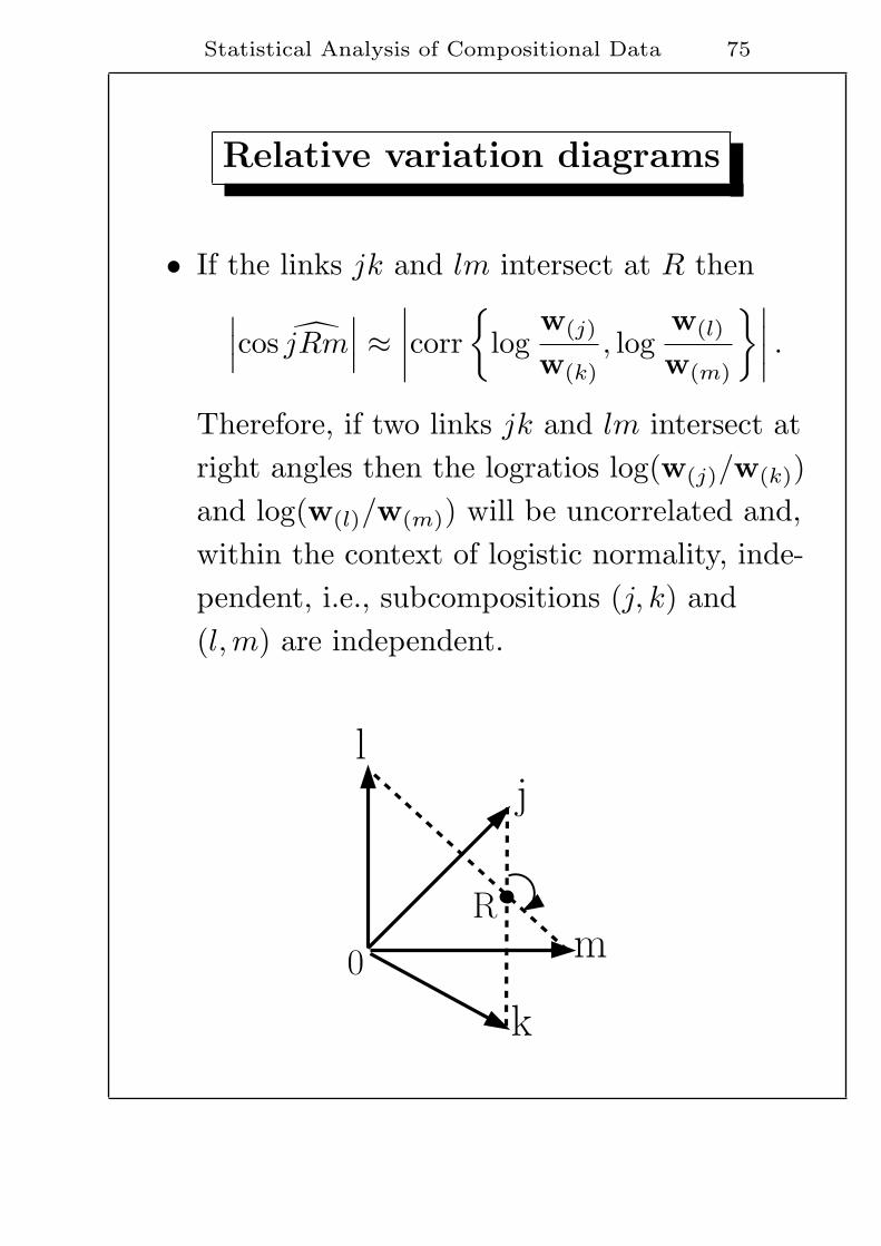
Relative variation diagrams
• If the links jk and lm intersect at R then∣∣∣cos jRm
∣∣∣ ≈∣∣∣∣corr
{log
w(j)
w(k), log
w(l)
w(m)
}∣∣∣∣ .
Therefore, if two links jk and lm intersect atright angles then the logratios log(w(j)/w(k))and log(w(l)/w(m)) will be uncorrelated and,within the context of logistic normality, inde-pendent, i.e., subcompositions (j, k) and(l,m) are independent.
j
k
0m
l
R

Statistical Analysis of Compositional Data 76
Relative variation diagrams
• The relative variation diagram for any sub-composition S is simply the subdiagramformed by selecting the vertices correspondingto the parts of the subcomposition and takingthe centroide OS of these vertices as thecenter of the subcompositional biplot.
Therefore, if a subset — say 1, . . . , C— ofvertices is approximately collinear then theassociated subcomposition has a ”composi-tional” one-dimensional structure.
j
k0
l0S
jk
0
l

Statistical Analysis of Compositional Data 77
Volcano H
• Parts: 1=Cl; 2=K2O; 3=P2O5; 4=TiO2; 5=SiO2.
• Variation matrix T
0 2, 784 4, 134 3, 970 2, 966
2, 784 0 0, 647 0, 645 0, 146
4, 134 0, 647 0 0, 071 0, 304
3, 970 0, 645 0, 071 0 0, 249
2, 966 0, 146 0, 304 0, 249 0
• Centered covariance matrix Γ
2, 134 −0, 221 −0, 803 −0, 743 −0, 368
−0, 221 0, 208 −0, 022 −0, 043 0, 079
−0, 803 −0, 022 0, 394 0, 337 0, 094
−0, 743 −0, 043 0, 337 0, 350 0, 099
−0, 368 0, 079 0, 094 0, 099 0, 096

Statistical Analysis of Compositional Data 78
Volcano H

Statistical Analysis of Compositional Data 79
Volcano H

Statistical Analysis of Compositional Data 80
Dimension-reducing techniques
Compositional PCA
Given a set of compositions w1, . . . ,wn of CD−1
with center g, the PCA will start looking for adirection —determined by a C-unitary composi-tion c1— such that the total variability of theC-orthogonal projections of w1, . . . ,wn on thecompositional straight line through g with direc-tion c1 will be maximum. And so on.
Property The compositional principal compo-nents of a set of compositions w1, . . . ,wn of CD−1
can be determined from the standard principalcomponents of the clr -transformed observationsclrw1, . . . , clrwn.

Statistical Analysis of Compositional Data 81
Compositional PCA
In this manner, the positive eigenvalues λ1 ≥ . . .
≥ λD−1 of the centered logratio covariance matrixΓ give the decomposition of totvarC , and thecorresponding unitary eigenvectors z∗1, . . . , z
∗D−1
determine the corresponding directionsclr−1z∗1, . . . , clr
−1z∗D−1 of the principal axes.

Statistical Analysis of Compositional Data 82
Skye Lavas
PC1: 0.4436 log A− 0.8154 log F + 0.3719 log M ≈ −0.7849

Statistical Analysis of Compositional Data 83
Volcano H
(Cl, K2O, P2O5, TiO2, SiO2)
PC1: (0.4246,0.1656,0.1264,0.1296,0.1538)’ (87.8%)
PC2: (0.1469,0.3836,0.1230,0.1182,0.2293)’ (acum 98.1%)

Statistical Analysis of Compositional Data 84
Dimension-reducing techniques
Subcomposition analysis
Let w1, . . . ,wn be a compositional data set ofCD−1, and let subS w1, . . . , subS wn be the set ofthe corresponding subcompositions of CC−1
associated to a subset S of parts 1, . . . , D. Then,the ratio
totvarC{subS w1, . . . , subS wn}totvarC{w1, . . . ,wn}
gives the proportion of total variabilitiy retainedby the subcompositions.
If the purpose of subcompositional analysis is toretain as much variability as possible for a givennumber C of parts, then we have to search forsubcompositions of this size which maximize thisratio.

Statistical Analysis of Compositional Data 85
Volcano H

Statistical Analysis of Compositional Data 86
Subcomposition analysis
Example Percentage of Cl, K2O, P2O5, TiO2
and SiO2 in 46 samples of volcanic rocks from ananonymous volcano H
? Total variability: totvarC = 3.1829.
? Total variability of 3-parts subcompositions:
Subcomposition Percentage
P2O5, TiO2, SiO2 6.53%
K2O, TiO2, SiO2 10.90%
K2O, P2O5, SiO2 11.48%
K2O, P2O5, TiO2 14.27%
Cl, K2O, SiO2 61.74%
Cl, TiO2, SiO2 75.25%
Cl, K2O, TiO2 77.48%
Cl, P2O5, SiO2 77.53%
Cl, K2O, P2O5 79.21%
Cl, P2O5, TiO2 85.61%

Statistical Analysis of Compositional Data 87
Zeros in compositional data
• Logratio methodology is incompatible withcomposition with zeros in one or more parts.
• Two kinds of zeros:
? Essential zeros: part completely absent.
? Rounded zeros: no quantifiable proportionhas been recorded.
• Treatment of essential zeros:
? Is it suitable to amalgamate some parts?
? Pre-classification: create initial groupsaccording to the number and location ofzeros, and analyze each group separately.
• Treatment of rounded zeros:
? Consider the zero values as missing values.
? Imputation: replace zero values by a smallamount using non-parametric orparametric techniques.
? Apply log-ratio methodology to replacedobservations of resulting data set.

Statistical Analysis of Compositional Data 88
Rounded zeros
Multiplicative replacement
Let be w = ccl (w1, . . . , wD)′ ∈ CD−1 anycomposition with some wj = 0 (rounded zero).
The multiplicative replacement replaces w bythe composition w(r) = ccl (w(r)
1 , . . . , w(r)D )′
defined by
if wj = 0 → w(r)j = δj ;
if wj 6= 0 → w(r)j = wj
(1−
∑wl=0
δl
).
where δj are the ”small” values replacing zerosparts.

Statistical Analysis of Compositional Data 89
Rounded zeros
Multiplicative replacement
• It is a ”natural” replacement.
• Ratio between two non-zero parts ispreserved.
• It is compatible with subcompositions,perturbation and power transformation.
• Covariance structure of subcompositions withno zeros is preserved.

Statistical Analysis of Compositional Data 90
Modeling compositional data
In practice, many of the probability densityfunctions (pdf) on the compositional space CD−1
will be defined from a pdf on the real space IRD−1.Then the alrj
−1 transformations will allow toinduce on the simplex SD the corresponding pdf.
The most important pdf on CD−1 are:
• The Dirichlet class.
• The (additive) logistic normal class.
• The (additive) logistic skewnormal class.
Definition A random composition w on CD−1
is said to have an additive logistic normaldistribution (aln) of parameters µ and Σ—written w ∼ LD−1(µ,Σ)— if the randomvector y = alrD w = log(w−D/wD) has aND−1(µ,Σ) on IRD−1.

Statistical Analysis of Compositional Data 91
Logistic normal distributions on CD−1
Property Let w be a random vector on CD−1.If alrD w ∼ ND−1(µ,Σ), then all the otherlogratio random vectors alrjw (j = 1, . . . , d) arenormally distributed.
Property Let w be a random composition onCD−1. Let wS be the random subcomposition onCC−1 corresponding to a subset S of C parts ofw. If w ∼ LD−1(µ,Σ), thenwS ∼ LC−1(µS ,ΣS), where µS and ΣS can beeasily calculated from µ and Σ.
Property Let w be a random vector on CD−1,which w ∼ LD−1(µ,Σ). If we perturb w by aconstant composition p ∈ CD−1, then theperturbed random vectorp⊕w ∼ LD−1(µ + alrD p,Σ).

Statistical Analysis of Compositional Data 92
Logistic normal distributions on CD−1
Estimation of parameters
To estimate the parameters µ and Σ of a randomcomposition w ∼ LD−1(µ,Σ) from a randomsample w1, . . . ,wn of w, we estimate by standardprocedures the vector mean and the covariancematrix of a multivariate normal distribution fromthe alrD-transformed random sample
y1 = alrDw1, . . . ,yn = alrD wn.
The maximum likelihood estimations of µ and Σare given by
µj =1n
n∑
i=1
yij ,
σjk =1n
n∑
i=1
(yij − µj)(yik − µk),
for j, k = 1, . . . , D − 1.

Statistical Analysis of Compositional Data 93
Predictive regions
Definition Let w be a random composition aln
distributed on CD−1. If µ and Σ are the estima-tes of the unknown parameters of w from arandom sample of size n, the 1− α predictiveregion is defined as{
w∗ ∈ CD−1 : (alrD w∗ − µ)′Σ−1
(alrD w∗ − µ) ≤ r2}
,
where r2 is a real number such that
Prob
[FD−1,n−(D−1) ≤
n(n− (D − 1))
(n2 − 1)(D − 1)r2
]= 1− α.
99% Predictive region - Skye lavas

Statistical Analysis of Compositional Data 94
Atypicality index
Definition If a random composition w on CD−1
is LD−1(µ,Σ) distributed, the atypicality indexof a composition w∗ ∈ CD−1 in relation to therandom composition w is defined as
Prob[χ2
D−1 ≤ (alrD w∗ − µ)′Σ−1(alrD w∗ − µ)]
.
Definition Let w be a random composition aln
distributed on CD−1. If µ and Σ are the estimatesof the unknown parameters of w from a randomsample w1, . . . ,wn of size n, the atypicality index
of a composition w∗ ∈ CD−1 in relation to thecompositional data set w1, . . . ,wn is defined as
Prob
[FD−1,n−(D−1) ≤ k(alrD w∗ − µ)′Σ
−1(alrD w∗ − µ)
],
where k =n(n−(D−1))
(n2−1)(D−1).

Statistical Analysis of Compositional Data 95
Compositional Regression
Artic lake
Sand, silt,clay composition of 39 sedimentsamples at different water depths in an Artic lake:
Num. Sand Silt Clay Depth (m)
S01 77.5 19.5 3.0 10.4
S02 71.9 24.9 3.2 11.7
.
.....
.
.....
.
..
S39 2.0 47.8 50.2 103.7
a. Is sediment composition dependent on waterdepth?
b. If so, how can we quantify the extent of thedependence?

Statistical Analysis of Compositional Data 96
Compositional Regression
• Compositions wi ∈ CD−1 regressing on a realconcomitant ti (i = 1, . . . , n):
wi = β0 ⊕ (ti ⊗ β1)⊗ εi (i = 1, . . . , n),
where
? β0: constant;
? β1: regression coefficient;
? εi (i = 1, . . . , n): errors.
• alr version of the regression model
alrwi = alr β0+tialr β1+alr εi (i = 1, . . . , n).
Can be reparametrized as
alrwi = α0 + tiα1 + εi (i = 1, . . . , n).

Statistical Analysis of Compositional Data 97
Compositional Regression
alrwi = α0 + tiα1 + εi (i = 1, . . . , n).
• Estimations α0 and α1 are obtained byapplication of the least squares method. Then
β0 = alr−1α0 , β1 = alr−1α1
• The error (residual) of wi (i = 1, . . . , n) willbe
ei = wi ª wi,
where wi = β0 ⊕ (ti ⊗ β1).
• Sum of squares of errors:
SSError =n∑
i=1
‖ei‖2C =n∑
i=1
(dC(wi, wi)
)2.
• Proportion of variability explained by thefitted linear regression model:
1− SSError
totvarC{w1, . . . ,wn} .

Statistical Analysis of Compositional Data 98
Artic lake
Num. Sand Silt Clay Depth (m)
S01 77.5 19.5 3.0 10.4
..
....
..
....
..
.
S39 2.0 47.8 50.2 103.7
• alr fitted simple linear regression model:
log(sand/clay) = 9.697− 2.743 log(depth) + ε1;
log(silt/clay) = 4.805− 1.096 log(depth) + ε2.
• Fitted regression model in S3:
cclL (sand, silt, clay)′ = (0.992849, 0.007145, 0.00006)′⊕
log(depth)⊗ (0.04604, 0.238291, 0.71505)′.
• Proportion of variability explained by the fitted
simple linear regression model:
1− 0.7006
2.4692= 0.716 ≡ 71.6%.

Statistical Analysis of Compositional Data 99
Artic lake
Num. Sand Silt Clay Depth (m)
S01 77.5 19.5 3.0 10.4
.
.....
.
.....
.
..
S39 2.0 47.8 50.2 103.7


![DOC HOLLIDAY MOLDS CURRENT PRICE LIST Prices Effective ... · DH282 22.98 Cup, Eight [8] Sided 5 4.5'T 4th DH390 84.98 Picture Frame, Collage 22 1O'Tx12"W 4th DH283 42.98 Picture](https://img.pdfslide.net/doc/110x75/600494b51abaaf5b831a1f1f/doc-holliday-molds-current-price-list-prices-effective-dh282-2298-cup-eight.jpg)


![Geometry Design of a Pitch Controlling Type Horizontal ... · % MS NACA 63-8xx 6 îï 7k , pq,r ¨ / Table 2]h . O 8 b ... 1 NACA63-824 0.0500 12.50 0.0611 27.4 2 NACA63-823 0.0675](https://img.pdfslide.net/doc/110x75/5adecf437f8b9a595f8eaa90/geometry-design-of-a-pitch-controlling-type-horizontal-ms-naca-63-8xx-6-7k-.jpg)