Embed Size (px)
Citation preview

compositional data Aitchison geometry exploratory analysis distributions on SD conclusions
Statistical analysis of compositional data
G. Mateu-Figueras
Dep. d’Informatica, Matematica Aplicada i EstadısticaUniversitat de Girona
February 26, 2014

compositional data Aitchison geometry exploratory analysis distributions on SD conclusions
Outline
1 compositional data
2 Aitchison geometry of the simplex
3 exploratory analysis
4 distributions on SD
5 conclusions

compositional data Aitchison geometry exploratory analysis distributions on SD conclusions
introduction
compositional data
compositional data are parts of some whole which onlycarry relative informationthe simplex (for κ a constant)
SD =
x = (x1, . . . , xD) ∈ RD
∣∣∣∣∣ xi > 0,D∑
i=1
xi = κ
standard representationfor D = 3: ternary diagram

compositional data Aitchison geometry exploratory analysis distributions on SD conclusions
examples
some compositional problems
MN blood system: frequencies of MM, NN and MN bloodtypes and the ethnic population. Despite the hightvariability, is there any stability in the data? do they followany genetic law?elections to the Parlament de Catalunya: the total votesachieved by each party in each counties. To characterizethe regions.skye lavas: relative proportions of A (Na2O + K2O), F(Fe2O3) and M (MgO) of 23 basalt specimens from the Isleof Skye. To describe the variability of the geochemicalcomposition.

compositional data Aitchison geometry exploratory analysis distributions on SD conclusions
difficulties
spurious correlations (Pearson, 1897)
x = (x1, . . . , xD)∑D
i=1 xi = κ cov(xi , x1)+· · ·+cov(xi , xD) = 0
sample x1 x2 x3 x4
1 0.1 0.2 0.1 0.62 0.2 0.2 0.3 0.33 0.3 0.3 0.1 0.3
cov x1 x2 x3 x4
x1 0.007 0.003 0.000 -0.010x2 0.003 0.002 -0.002 -0.003x3 0.000 -0.002 0.009 -0.007x4 -0.010 -0.003 -0.007 0.020
corr x1 x2 x3 x4
x1 1.000 0.866 0.000 -0.866x2 0.866 1.000 -0.500 -0.500x3 0.000 -0.500 1.000 -0.500x4 -0.866 -0.500 -0.500 1.000

compositional data Aitchison geometry exploratory analysis distributions on SD conclusions
difficulties
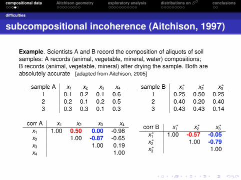
subcompositional incoherence (Aitchison, 1997)
Example. Scientists A and B record the composition of aliquots of soilsamples: A records (animal, vegetable, mineral, water) compositions;B records (animal, vegetable, mineral) after drying the sample. Both areabsolutely accurate [adapted from Aitchison, 2005]
sample A x1 x2 x3 x4
1 0.1 0.2 0.1 0.62 0.2 0.1 0.2 0.53 0.3 0.3 0.1 0.3
sample B x∗1 x∗2 x∗31 0.25 0.50 0.252 0.40 0.20 0.403 0.43 0.43 0.14
corr A x1 x2 x3 x4
x1 1.00 0.50 0.00 -0.98x2 1.00 -0.87 -0.65x3 1.00 0.19x4 1.00
corr B x∗1 x∗2 x∗3x∗1 1.00 -0.57 -0.05x∗2 1.00 -0.79x∗3 1.00

compositional data Aitchison geometry exploratory analysis distributions on SD conclusions
difficulties
subcompositional incoherence (Aitchison, 1997)
Example. Scientists A and B record the composition of aliquots of soilsamples: A records (animal, vegetable, mineral, water) compositions;B records (animal, vegetable, mineral) after drying the sample. Both areabsolutely accurate [adapted from Aitchison, 2005]
sample A x1 x2 x3 x4
1 0.1 0.2 0.1 0.62 0.2 0.1 0.2 0.53 0.3 0.3 0.1 0.3
sample B x∗1 x∗2 x∗31 0.25 0.50 0.252 0.40 0.20 0.403 0.43 0.43 0.14
corr A x1 x2 x3 x4
x1 1.00 0.50 0.00 -0.98x2 1.00 -0.87 -0.65x3 1.00 0.19x4 1.00
corr B x∗1 x∗2 x∗3x∗1 1.00 -0.57 -0.05x∗2 1.00 -0.79x∗3 1.00

compositional data Aitchison geometry exploratory analysis distributions on SD conclusions
principles
scale invariance: the analysis should not depend on theclosure constant κ
f (αx) = f (x) , α > 0
subcompositional coherence: studies performed onsubcompositions should not stand in contradiction withthose performed on the full composition

compositional data Aitchison geometry exploratory analysis distributions on SD conclusions
Euclidean space structure of SD
for x,y ∈ SD, α ∈ R, and C is the closure operation
perturbation: x⊕ y = C(x1y1, . . . , xDyD)
powering: α x = C(xα1 , . . . , xαD )
inner product:
〈x,y〉a =1D
∑i<j
lnxi
xjln
yi
yj
associated norm and distance:
‖x‖2a =1D
∑i<j
(ln
xi
xj
)2
; d2a (x,y) =
1D
∑i<j
(ln
xi
xj− ln
yi
yj
)2

compositional data Aitchison geometry exploratory analysis distributions on SD conclusions
orthonormal coordinates
orthonormal basis on SD: e1,e2, . . . ,eD−1 (not unique)coordinates in this basis for x ∈ SD or ilr coordinatesx∗ = (〈x,e1〉a, . . . , 〈x,eD−1〉a)
example:e1 = C(exp( 1√
6, 1√
6, −2√
6)), e2 = C(exp( 1√
2, −1√
2,0))
x∗ =
(√23
ln(x1 · x2)1/2
x3,
1√2
lnx1
x2
)Egozcue et al. (2003)
compositional operations are reduced to ordinary vectoroperations when representing compositions by theircoordinatesthe principle of working on coordinates
compositional data Aitchison geometry exploratory analysis distributions on SD conclusions
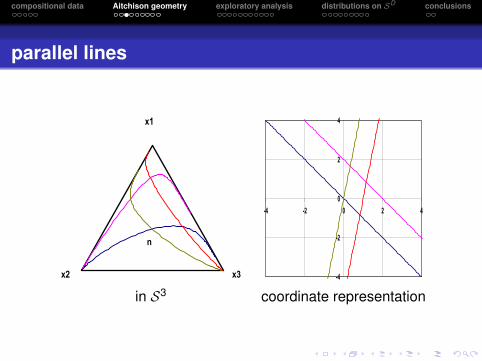
parallel lines
x2
x1
x3
n
-4
-2
0
2
4
-4 -2 0 2 4
in S3 coordinate representation

compositional data Aitchison geometry exploratory analysis distributions on SD conclusions
circles and ellipses
-2
-1
0
1
2
3
4
-2 -1 0 1 2 3
in S3 coordinate representation

compositional data Aitchison geometry exploratory analysis distributions on SD conclusions
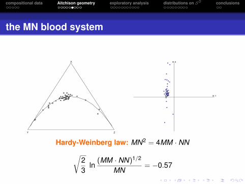
the MN blood system
√23
ln(MM · NN)1/2
MN= −0.57
compositional data Aitchison geometry exploratory analysis distributions on SD conclusions
the MN blood system
Hardy-Weinberg law: MN2 = 4MM · NN√23
ln(MM · NN)1/2
MN= −0.57

compositional data Aitchison geometry exploratory analysis distributions on SD conclusions
building an orthonormal basis
using sequential binary partitions (SBP)
example: sequential binary partition for x ∈ S5;coordinates in the corresponding orthonormal basis
order x1 x2 x3 x4 x5 coordinate
1 +1 −1 +1 +1 −1 x∗1 =√
3·23+2 ln (x1·x3·x4)
1/3
(x2·x5)1/2
2 0 +1 0 0 −1 x∗2 =√
1·11+1 ln x2
x5
3 +1 0 −1 −1 0 x∗3 =√
1·21+2 ln x1
(x3·x4)1/2
4 0 0 +1 −1 0 x∗4 =√
1·11+1 ln x3
x4

compositional data Aitchison geometry exploratory analysis distributions on SD conclusions
coordinates⇒ balances
coordinates in an orthonormal basis obtained from a sequentialbinary partition:
x∗i =
√ri · si
ri + siln
(∏
j∈Rixj)
1/ri
(∏`∈Si
x`)1/si
where i = order of partition, Ri and Si index sets,ri the number of indices in Ri , si the number in Si
Egozcue, Pawlowsky-Glahn (2005)

compositional data Aitchison geometry exploratory analysis distributions on SD conclusions
Log-ratio approach (Aitchison, 1980-86)
log-ratio transformations introduced by J. Aitchison:
alr: SD → RD−1, alr(x) =(
ln x1xD, . . . , ln xD−1
xD
)drawback: not an isometry
clr: SD → RD, clr(x) =(
ln x1g(x) , . . . , ln
xDg(x)
),
g(x) =D∏
i=1x1/D
i
drawback: a constrained transformed vector

compositional data Aitchison geometry exploratory analysis distributions on SD conclusions
the treatment of zeros
case 1: the part with zeros is not important for the study⇒ the part should be omitted
case 2: the part is important, the zeros are essential⇒ divide the sample into two or more populations,according to the presence/absence of zeros
case 3: the part is important, the zeros are rounded zeros⇒ use imputation techniques
for a review, see Martın-Fernandez et al. (2011)

compositional data Aitchison geometry exploratory analysis distributions on SD conclusions
center and variability
let X = xi = (xi1, . . . , xiD) ∈ SD : i = 1, . . . ,n
center (closed geometric mean) of X:
g = C(g1,g2, . . . ,gD), with gj =
(n∏
i=1
xij
)1/n
total variance of X: TotVar[X] = 1n
∑ni=1 d2
a (xi ,g)
variation array of X:
− var[ln x1
x2
]· · · var
[ln x1
xD
]E[ln x1
x2
]−
. . ....
.... . . − var
[ln xD−1
xD
]E[ln x1
xD
]· · · E
[ln xD−1
xD
]−

compositional data Aitchison geometry exploratory analysis distributions on SD conclusions
example: ParlCat2010 data set
votes achieved by PP, CiU, SI, C’s, ERC, PSC, ICV
g = (0.097,0.505,0.044,0.017,0.102,0.179,0.056)

compositional data Aitchison geometry exploratory analysis distributions on SD conclusions
clr biplot
graphical display of a multivariate data set (individuals andvariables)clr-biplotparticular rules of interpretation
‖ray‖ ≈ variance clr component‖link‖ ≈ variance logratioperpendicular links⇒ possible incorrelated logratiosparallel links⇒ possible hight correlated logratioscoincident vertices⇒ two redundant partscollinear vertices⇒ possible one-dimensional variability
Aitchison and Greenacre (2002)

compositional data Aitchison geometry exploratory analysis distributions on SD conclusions
example: ParlCat2010 data set (explains 86% variance)
var(
ln(
ICVg
))= 0.0417 var
(ln(
C′sg
))= 0.2898

compositional data Aitchison geometry exploratory analysis distributions on SD conclusions
example: ParlCat2010 data set (explains 86% variance)
var(
ln(
ICVg
))= 0.0417 var
(ln(
C′sg
))= 0.2898

compositional data Aitchison geometry exploratory analysis distributions on SD conclusions
example: ParlCat2010 data set (explains 86% variance)
var(ln( SI
C′s
))= 0.8915 var
(ln( CiU
ERC
))= 0.0732

compositional data Aitchison geometry exploratory analysis distributions on SD conclusions
example: ParlCat2010 data set (explains 86% variance)
corr(
ln(
C′sERC
), ln(PSC
ICV
))= −0.041

compositional data Aitchison geometry exploratory analysis distributions on SD conclusions
example: ParlCat2010 data set (explains 86% variance)

compositional data Aitchison geometry exploratory analysis distributions on SD conclusions
coda-dendrogram
to visualizesequential binary partitioncenter of each balanceproportion of the sample total variance corresponding toeach balance.summary statistics of each balance (box-plot ofpercentiles 5, 25, 50, 75, 95)adequate to represent different groups
Pawlowsky-Glahn and Egozcue (2011)

compositional data Aitchison geometry exploratory analysis distributions on SD conclusions
example: ParlCat2010 data set

compositional data Aitchison geometry exploratory analysis distributions on SD conclusions
example: ParlCat2010 data set

compositional data Aitchison geometry exploratory analysis distributions on SD conclusions
logistic normal (Aitchison 1980-86)
x : Ω −→ SD
transform x to RD−1 using a log-ratio transformationdefine the density of the transformed vector and go backto SD using the change of variable theoremthe result is a density function for x with respect to λ on SD
⇓(Aitchison, 1997)
E [x] is not a meaningful measure of central locationcen[x] is the alternative which minimizes E[d2
a (x, cen[x])]

compositional data Aitchison geometry exploratory analysis distributions on SD conclusions
densities and measures
on SD: density functions expressed with respect to theAitchison measure λa
density functions of the vector of coordinates with respectto λ.
dλ/dλa =√
D x1x2 · · · xD, λa(A) = λ(A∗)

compositional data Aitchison geometry exploratory analysis distributions on SD conclusions
densities and measures
on SD: density functions expressed with respect to theAitchison measure λa
density functions of the vector of coordinates with respectto λ.
dλ/dλa =√
D x1x2 · · · xD, λa(A) = λ(A∗)

compositional data Aitchison geometry exploratory analysis distributions on SD conclusions
normal on SD
x : Ω −→ SD
a random composition x is normally distributed on SD withparameters µ and Σ if its density function is
fx(x) = (2π)−(D−1)/2|Σ|−1/2 exp[−1
2(x∗ − µ∗)′Σ−1 (x∗ − µ∗)
]usual normal density applied to coordinates x∗ and fx = dP
dλa
µ = Ea[x] = cen[x]
Mateu-Figueras et al (2013)
compositional data Aitchison geometry exploratory analysis distributions on SD conclusions
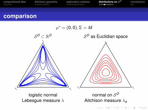
comparison
µ∗ = (0,0),Σ = Id
SD ⊂ RD SD as Euclidian spacex
1
x2
x3
x1
x2
x3
logistic normal normal on SD
Lebesgue measure λ Aitchison measure λa

compositional data Aitchison geometry exploratory analysis distributions on SD conclusions
invariance under perturbation
p=(0.93, 0.05,0.02) x∗ =(
1√2
ln(
x1x2
), 1√
6ln(
x1x2x3x3
))x
1
x2
x3
−3 −2 −1 0 1 2 3 4
−2
−1
0
1
2
3
normal on S3 coordinate representation
µ∗ = (−0.5,−0.5), µ∗ = (1.5,1.5), Σ = Id
compositional data Aitchison geometry exploratory analysis distributions on SD conclusions
tests of normality on SD
H0: the sample of coordinates comes from a multivariatenormal distribution
based on empirical distribution function (EDF) testsAnderson-Darling, Cramer-von Mises and Watson statisticsthree possible cases
all (D − 1) marginal, univariate distributionsall (D − 1)(D − 2)/2 bivariate angle distributionsthe (D − 1)-dimensional radius distribution
problem: dependence of the orthonormal basis

compositional data Aitchison geometry exploratory analysis distributions on SD conclusions
example: aphyric Skye lavas
X=(A,F,M) composition of 23 basalt specimens from the Isle ofSkye (Aitchison,1986)
µ∗ = (0.555,0.639) Σ =
(0.126 −0.229−0.229 0.456
)F
A M

compositional data Aitchison geometry exploratory analysis distributions on SD conclusions
kernel density estimation
the normal on SD for the kernel in the density estimatorinvariance with respect to the orthonormal basis
A
F M
90
90
90
75
75
75
50
50
50
25
25
25
10
10
10
−2 −1 0 1−1
0
1
2
3
y1
y2
Chacon et al (2010)

compositional data Aitchison geometry exploratory analysis distributions on SD conclusions
other distributions on SD
the skew-normal distribution on SD
the Dirichlet distributionthe shifted-scaled Dirichlet distribution...

compositional data Aitchison geometry exploratory analysis distributions on SD conclusions
conclusions
treat compositional data (CoDa) in the simplex, with itsspecific geometrydo not apply ordinary multivariate statistics directly toCoDathe simplex has an Euclidean structure: orthonormalcoordinates are availablemultivariate statistical models and methods work properlyon coordinates of CoDaproblem (or advantage): interpretation of coordinates

compositional data Aitchison geometry exploratory analysis distributions on SD conclusions
referencesAitchison, J. (1986): The statistical analysis of compositional data. Monographs onstatistics and applied Probability: Chapman and Hall, London.Aitchison, J., Greenacre, M. (2002): Biplots for compositional data .Journal of theRoyal Statistical Society, Series C (Applied Statistics) 51 (4), 375–392. 2002Billheimer, D.; Guttorp, P.; Fagan, W. (2001): Statistical interpretation of speciescomposition.J. Am. Statistical Ass., 96(456), 1205–1214.Chacon, J.E.; Mateu-Figueras, G.; Martın-Fernandez, J.A. (2010): Gaussian kernels fordensity estimation with compositional data.Computers and Geosciences., 37, 702–711.Egozcue, J.J.; Pawlowsky-Glahn, V. (2005): Groups of parts and their balances incompositional data analysis. Math. Geol., 37(7), 795–828.Egozcue, J.J.; Pawlowsky-Glahn, V., Mateu-Figueras, G.; Barcelo-Vidal, C. (2003):Isometric logratio transformations for compositional data analysis. MathematicalGeology, 35(3), 279–300.Martın-Fernandez, J.A.; Palarea-Albaladejo, J.; Olea, R.A. (2011): Dealing with zeros.In Pawlowsky-Glahn, V. and Buccianti A. (Eds.) Compositional Data Analysis: Theoryand Applications, Wiley, Chichester UK.Mateu-Figueras, G.; Pawlowsky-Glahn, V.; Egozcue, J.J. (2013): The normaldistribution in some constrained sample spaces. SORT, 37(1),29-56.Pawlowsky-Glahn, V.; Egozcue, J.J. (2001): Geometric approach to statistical analysison the simplex. SERRA, 15(5), 384–398.Pawlowsky-Glahn, V.; Egozcue, J.J. (2011): Exploring Compositional Data with theCoda-Dendrogram, Austrian Journal of Statistics, 40, 1-2.