Statistical Analysis of Persistent Homology

Genki Kusano (Tohoku University, D1)

Topology and Computer 2016, Oct 28 @ Akita.

Collaborators：Kenji Fukumizu (The Institute of Statistical Mathematics）Yasuaki Hiraoka (Tohoku University, AIMR)

Persistence weighted Gaussian kernel for topological data analysis. Proceedings of the 33rd ICML, pp. 2004–2013, 2016

• Interests : Applied topology, topological data analysisB3 : Homology group, homological algebraB4 : Persistent homology, computational homology M1 : Applied topology to sensor network “Relative interleavings and applications to sensor networks”, JJIAM, 33(1),99-120, 2016.M2 : Statistics, machine learning, kernel methods “Persistence weighted Gaussian kernel for topological data analysis”, ICML, pp. 2004–2013, 2016.D1(now) : Time series analysis, dynamics, information geometry, …

Self introduction

• Announcement : Joint Mathematics Meetings, January 4, 2017, Atlanta ★Statistical Methods in Computational Topology and Applications

　Sheaves in Topological Data Analysis

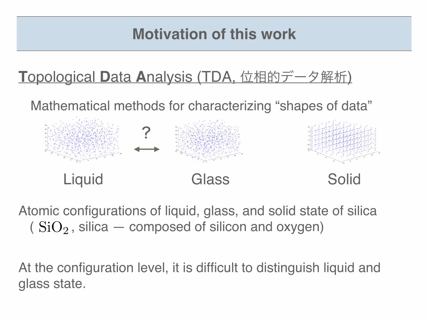
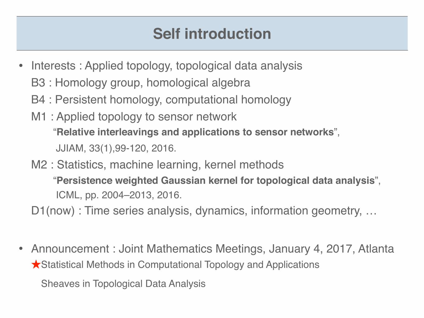
Topological Data Analysis (TDA, 位相的データ解析)

Mathematical methods for characterizing “shapes of data”

−10−5

05

1015

−5

0

5

10−15

−10

−5

0

5

10

05

1015

2025

05

1015

20250

5

10

15

20

25

30

05

1015

2025

05

1015

20250

5

10

15

20

25

30

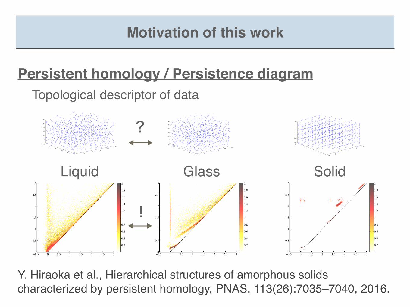
Liquid　　　　 　 Glass 　　　 　 Solid

Motivation of this work

Atomic configurations of liquid, glass, and solid state of silica ( , silica — composed of silicon and oxygen)SiO2

At the configuration level, it is difficult to distinguish liquid and glass state.

？

[A2]

[A2]

−0.5 0 0.5 1 1.5 2 2.5 30

0.5

1

1.5

2

2.5

3

Mu

ltip

licity

0.2

0.4

0.6

0.8

1

1.2

1.4

1.6

1.8

2

[A2]

[A2]

−0.5 0 0.5 1 1.5 2 2.5 30

0.5

1

1.5

2

2.5

3

Mu

ltip

licity

0.2

0.4

0.6

0.8

1

1.2

1.4

1.6

1.8

2

[A2]

[A2]

−0.5 0 0.5 1 1.5 2 2.5 30

0.5

1

1.5

2

2.5

3

Mu

ltip

licity

0.2

0.4

0.6

0.8

1

1.2

1.4

1.6

1.8

2

−10−5

05

1015

−5

0

5

10−15

−10

−5

0

5

10

05

1015

2025

05

1015

20250

5

10

15

20

25

30

05

1015

2025

05

1015

20250

5

10

15

20

25

30

Persistent homology / Persistence diagram　Topological descriptor of data

Y. Hiraoka et al., Hierarchical structures of amorphous solids characterized by persistent homology, PNAS, 113(26):7035–7040, 2016.

Motivation of this work

Liquid　　　　 　 Glass 　　　 　 Solid

！

？

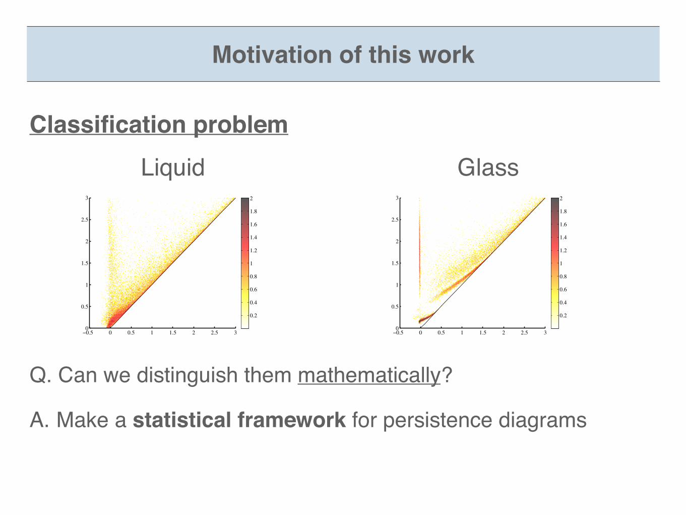
Liquid　　　　　 　 Glass 　

[A2]

[A2]

−0.5 0 0.5 1 1.5 2 2.5 30

0.5

1

1.5

2

2.5

3

Multi

plic

ity

0.2

0.4

0.6

0.8

1

1.2

1.4

1.6

1.8

2

[A2]

[A2]

−0.5 0 0.5 1 1.5 2 2.5 30

0.5

1

1.5

2

2.5

3

Multi

plic

ity

0.2

0.4

0.6

0.8

1

1.2

1.4

1.6

1.8

2

Classification problem

Q. Can we distinguish them mathematically?

A. Make a statistical framework for persistence diagrams

Motivation of this work

Section 1What is a persistence diagram

-2 0 2 4

-20

24

x1

y1

-2 0 2 4

-20

24

x1

y1

-2 0 2 4

-20

24

x1

y1

-2 0 2 4

-20

24

x1

y1

-2 0 2 4

-20

24

x1

y1

�

-2 0 2 4

-20

24

x1

y1

X

b�

d�

b�

x�d�

R2

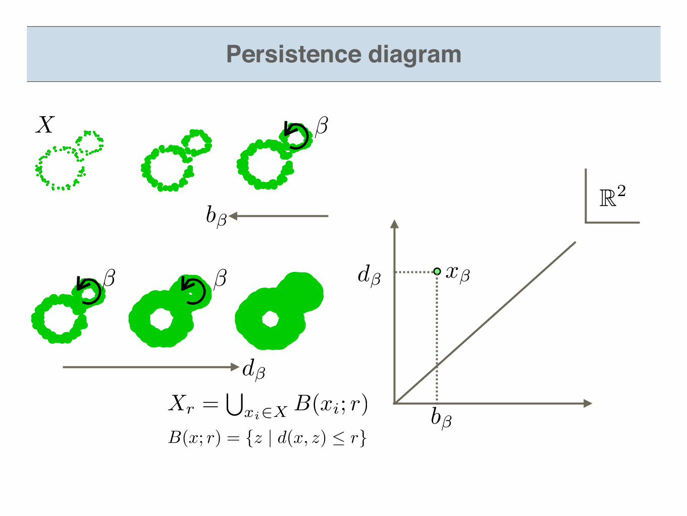
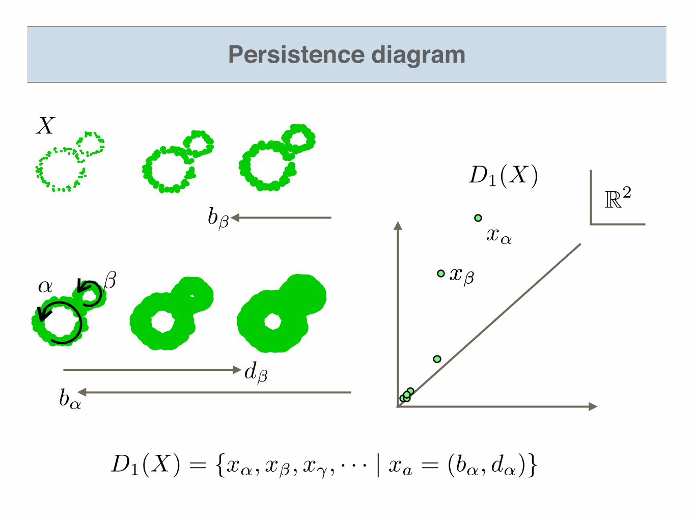
Persistence diagram

� �

X

r

=S

xi2X

B(xi

; r)

B(x; r) = {z | d(x, z) r}

-2 0 2 4

-20

24

x1

y1

-2 0 2 4

-20

24

x1

y1

-2 0 2 4

-20

24

x1

y1

-2 0 2 4

-20

24

x1

y1

-2 0 2 4

-20

24

x1

y1

↵

-2 0 2 4

-20

24

x1

y1

X

D1(X) = {x↵, x� , x� , · · · | xa = (b↵, d↵)}

d�b↵

D1(X)

x�

x↵

x�

R2

b�

Persistence diagram

�

Definition of persistence diagram

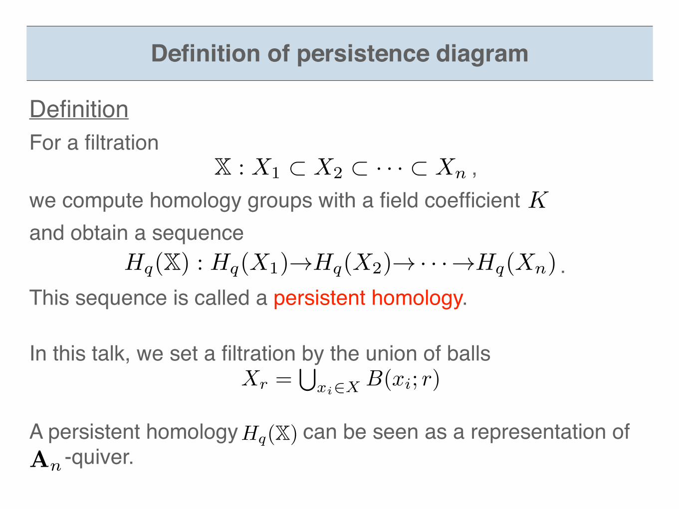
For a filtration ,we compute homology groups with a field coefficient and obtain a sequence .

Definition

This sequence is called a persistent homology.

A persistent homology can be seen as a representation of -quiver.

Hq(X)An

In this talk, we set a filtration by the union of ballsX

r

=S

xi2X

B(xi

; r)

X : X1 ⇢ X2 ⇢ · · · ⇢ Xn

Hq(X) : Hq(X1)!Hq(X2)! · · ·!Hq(Xn)

K

Hq(X) ⇠=M

i2I

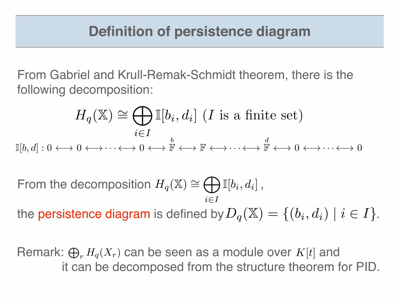
I[bi, di] (I is a finite set)

From the decomposition　 ,

the persistence diagram is defined by .

Hq(X) ⇠=M

i2I

I[bi, di]

Dq(X) = {(bi, di) | i 2 I}

I[b, d] : 0 ! 0 ! · · · ! 0 !bF ! F ! · · · !

dF ! 0 ! · · · ! 0

From Gabriel and Krull-Remak-Schmidt theorem, there is the following decomposition:

Definition of persistence diagram

Remark: 　　　　 can be seen as a module over and it can be decomposed from the structure theorem for PID.

K[t]L

r Hq(Xr)

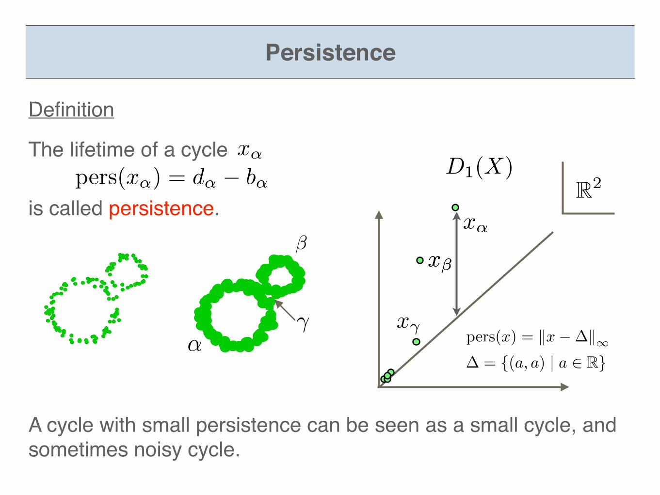
The lifetime of a cycle

is called persistence.

-2 0 2 4

-20

24

x1

y1

-2 0 2 4

-20

24

x1

y1

�

↵

Persistence

pers(x↵) = d↵ � b↵

Definition

-2 0 2 4

-20

24

x1

y1

x↵D1(X)

x�

x↵

x�

R2

pers(x) = kx��k1� x�

A cycle with small persistence can be seen as a small cycle, and sometimes noisy cycle.

� = {(a, a) | a 2 R}

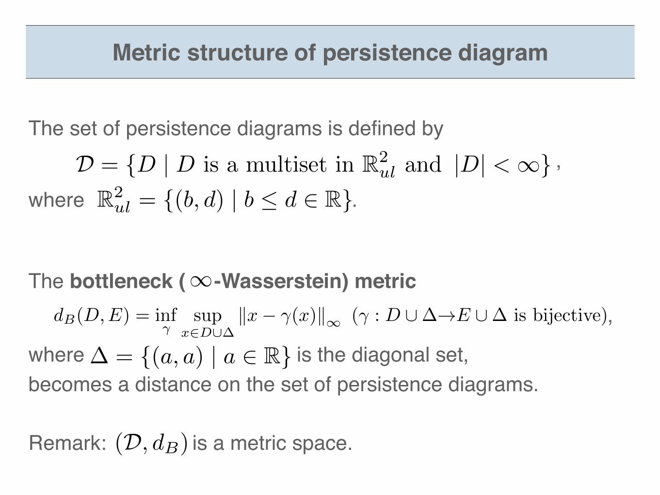
Remark: is a metric space.

Metric structure of persistence diagram

(D, dB)

The set of persistence diagrams is defined by ,

where 　 .R2ul = {(b, d) | b d 2 R}

D = {D | D is a multiset in R2ul and |D| < 1}

The bottleneck ( -Wasserstein) metric ,

where is the diagonal set,becomes a distance on the set of persistence diagrams.

� = {(a, a) | a 2 R}

d

B

(D,E) = inf�

supx2D[�

kx� �(x)k1 (� : D [�!E [� is bijective)

1

Stability theorem

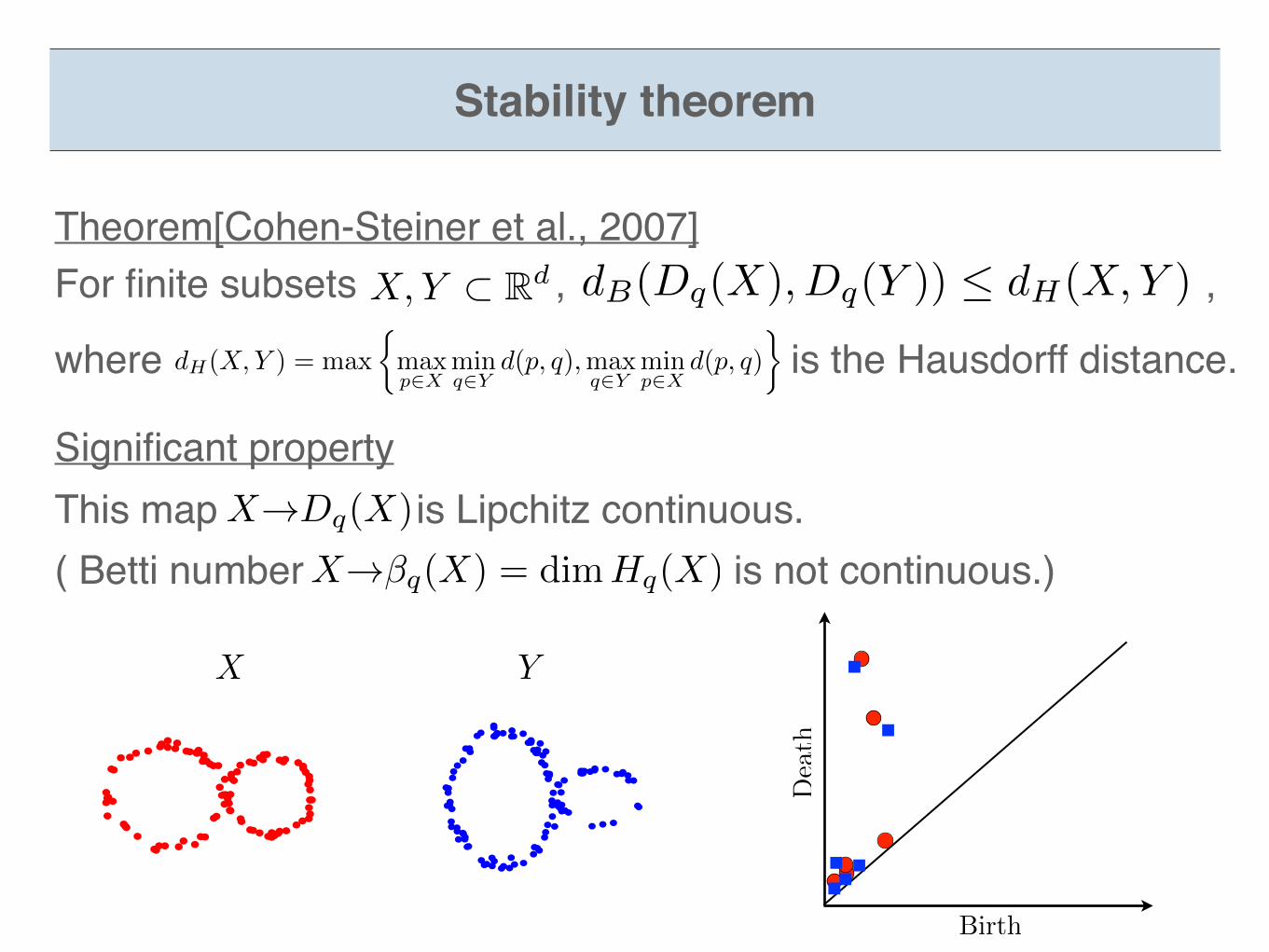
This map is Lipchitz continuous.( Betti number is not continuous.)

Significant propertyX!Dq(X)

X!�q(X) = dimHq(X)

-10 -5 0 5 10 15

-10

-50

510

15

x1

y1

-10 -5 0 5 10 15

-10

-50

510

15

x1

y1

X Y

Birth

Death

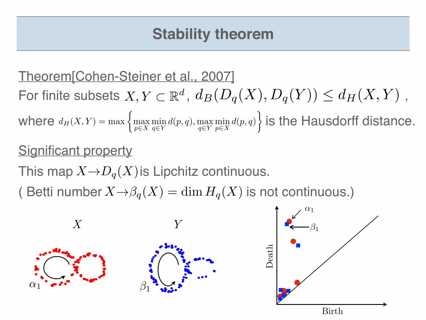
For finite subsets , 　　　　　　　　　　　　　　　 ,

where　　　　　　　　　　　　　　　 is the Hausdorff distance.dH(X,Y ) = max

⇢max

p2Xmin

q2Yd(p, q),max

q2Ymin

p2Xd(p, q)

�

Theorem[Cohen-Steiner et al., 2007]dB(Dq(X), Dq(Y )) dH(X,Y )X,Y ⇢ Rd

Stability theorem

-10 -5 0 5 10 15

-10

-50

510

15

x1

y1

-10 -5 0 5 10 15

-10

-50

510

15

x1

y1

X Y

�1↵1

Birth

Death

↵1

�1

This map is Lipchitz continuous.( Betti number is not continuous.)

Significant propertyX!Dq(X)

X!�q(X) = dimHq(X)

For finite subsets , 　　　　　　　　　　　　　　　 ,

where　　　　　　　　　　　　　　　 is the Hausdorff distance.dH(X,Y ) = max

⇢max

p2Xmin

q2Yd(p, q),max

q2Ymin

p2Xd(p, q)

�

Theorem[Cohen-Steiner et al., 2007]dB(Dq(X), Dq(Y )) dH(X,Y )X,Y ⇢ Rd

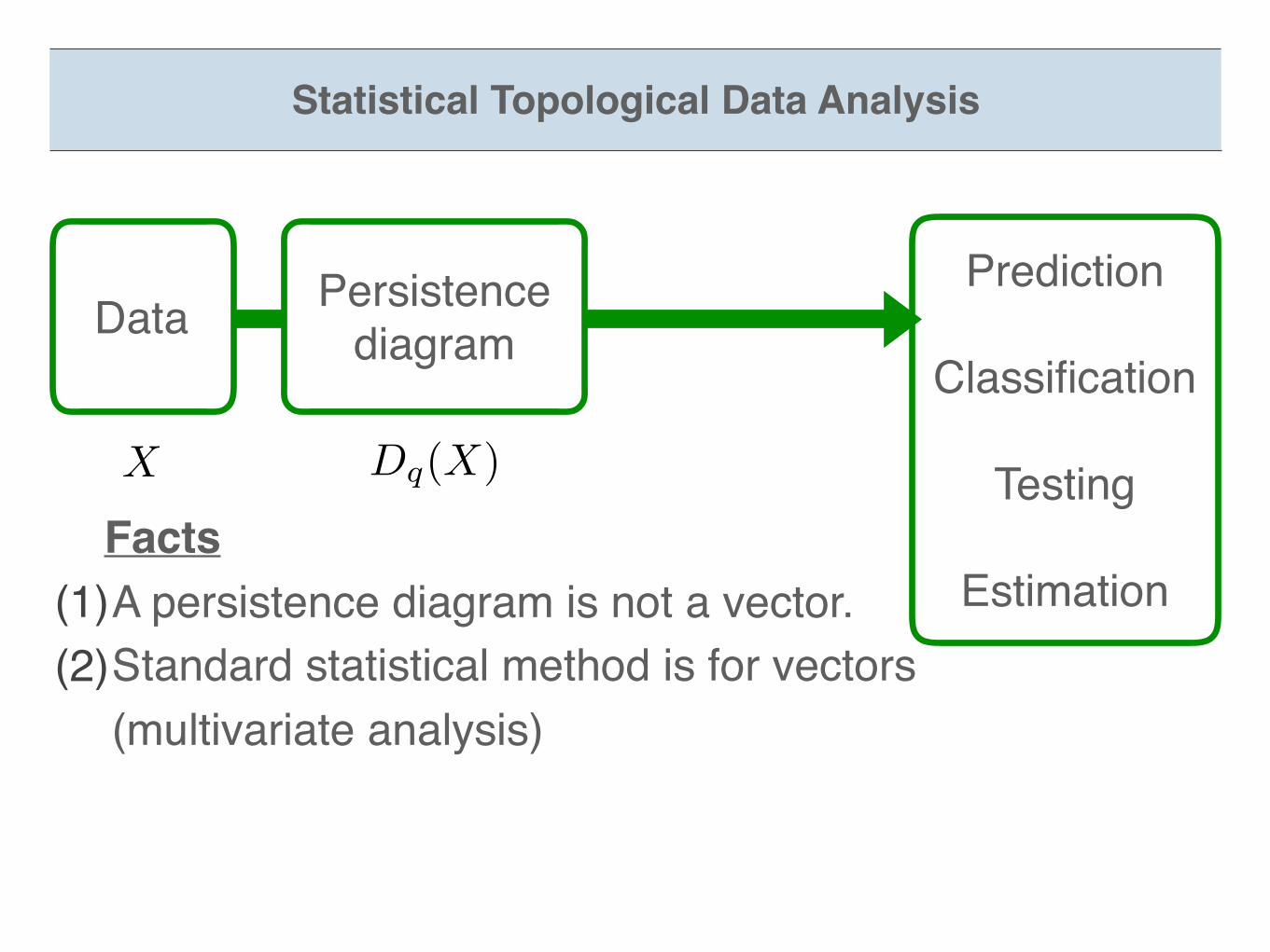
Statistical Topological Data Analysis

Data Persistence diagram

X Dq(X)

Prediction

Classification

Testing

Estimation Facts(1)A persistence diagram is not a vector.(2)Standard statistical method is for vectors

(multivariate analysis)

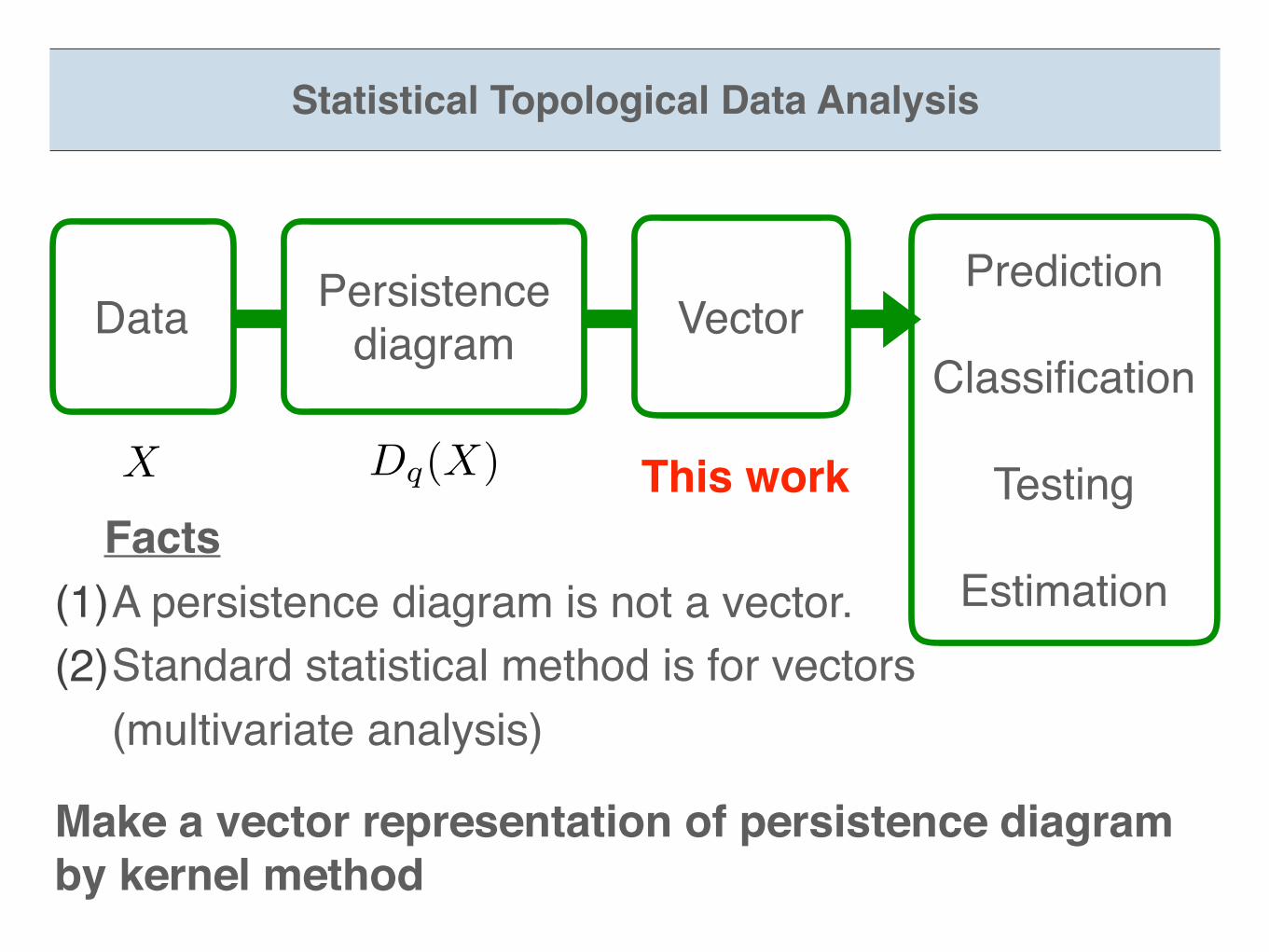
Statistical Topological Data Analysis

Data Persistence diagram

X Dq(X)

VectorPrediction

Classification

Testing

Estimation Facts(1)A persistence diagram is not a vector.(2)Standard statistical method is for vectors

(multivariate analysis)

Make a vector representation of persistence diagram by kernel method

This work

Section 2Kernel method

~Statistical method for non-vector data~

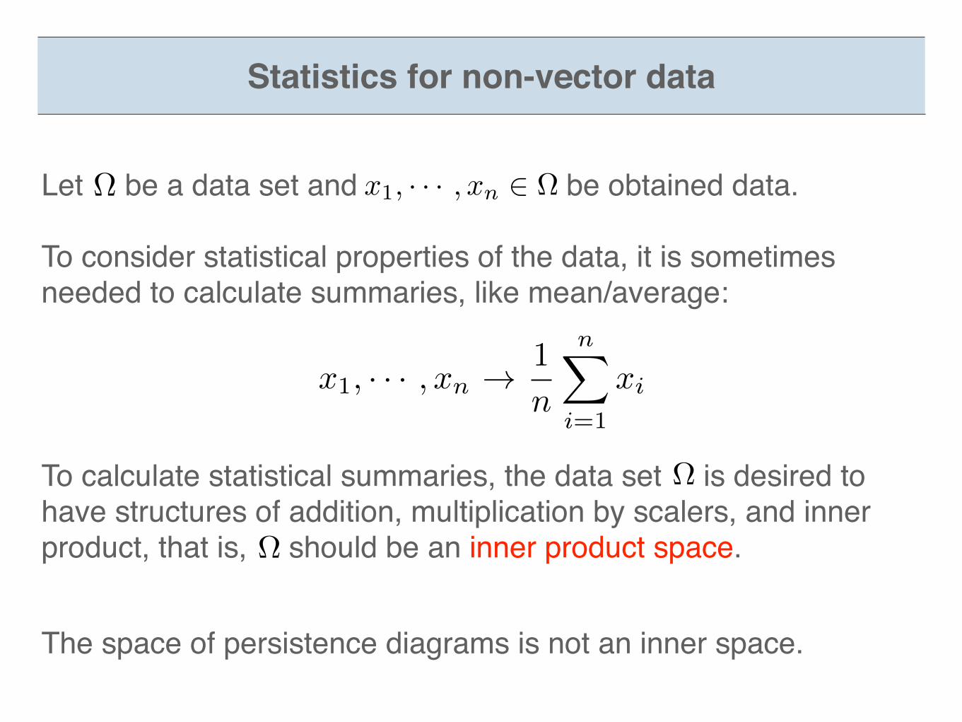
Statistics for non-vector data

Let be a data set and be obtained data.

To consider statistical properties of the data, it is sometimes needed to calculate summaries, like mean/average:

⌦ x1, · · · , xn 2 ⌦

x1, · · · , xn ! 1

n

nX

i=1

xi

To calculate statistical summaries, the data set is desired to have structures of addition, multiplication by scalers, and inner product, that is, should be an inner product space.⌦

⌦

The space of persistence diagrams is not an inner space.

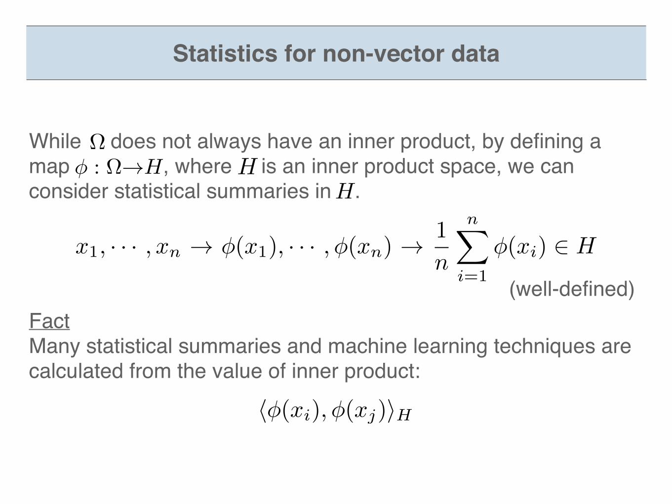
While does not always have an inner product, by defining a map , where is an inner product space, we can consider statistical summaries in .

⌦� : ⌦!H H

H

x1, · · · , xn ! �(x1), · · · ,�(xn) !1

n

nX

i=1

�(xi) 2 H

(well-defined)FactMany statistical summaries and machine learning techniques are calculated from the value of inner product:

h�(xi),�(xj)iH

Statistics for non-vector data

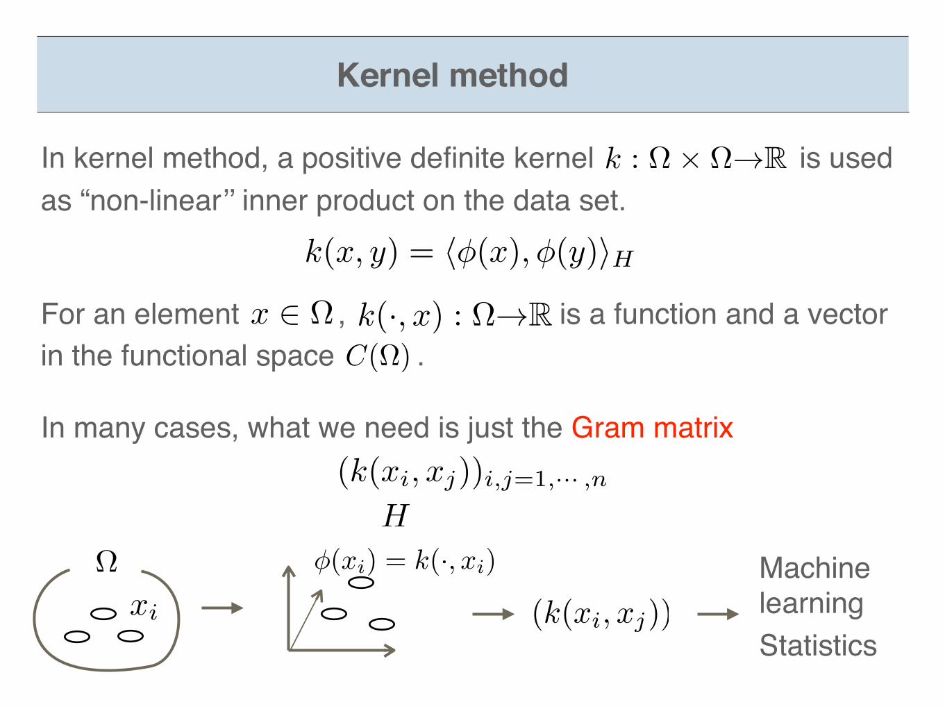
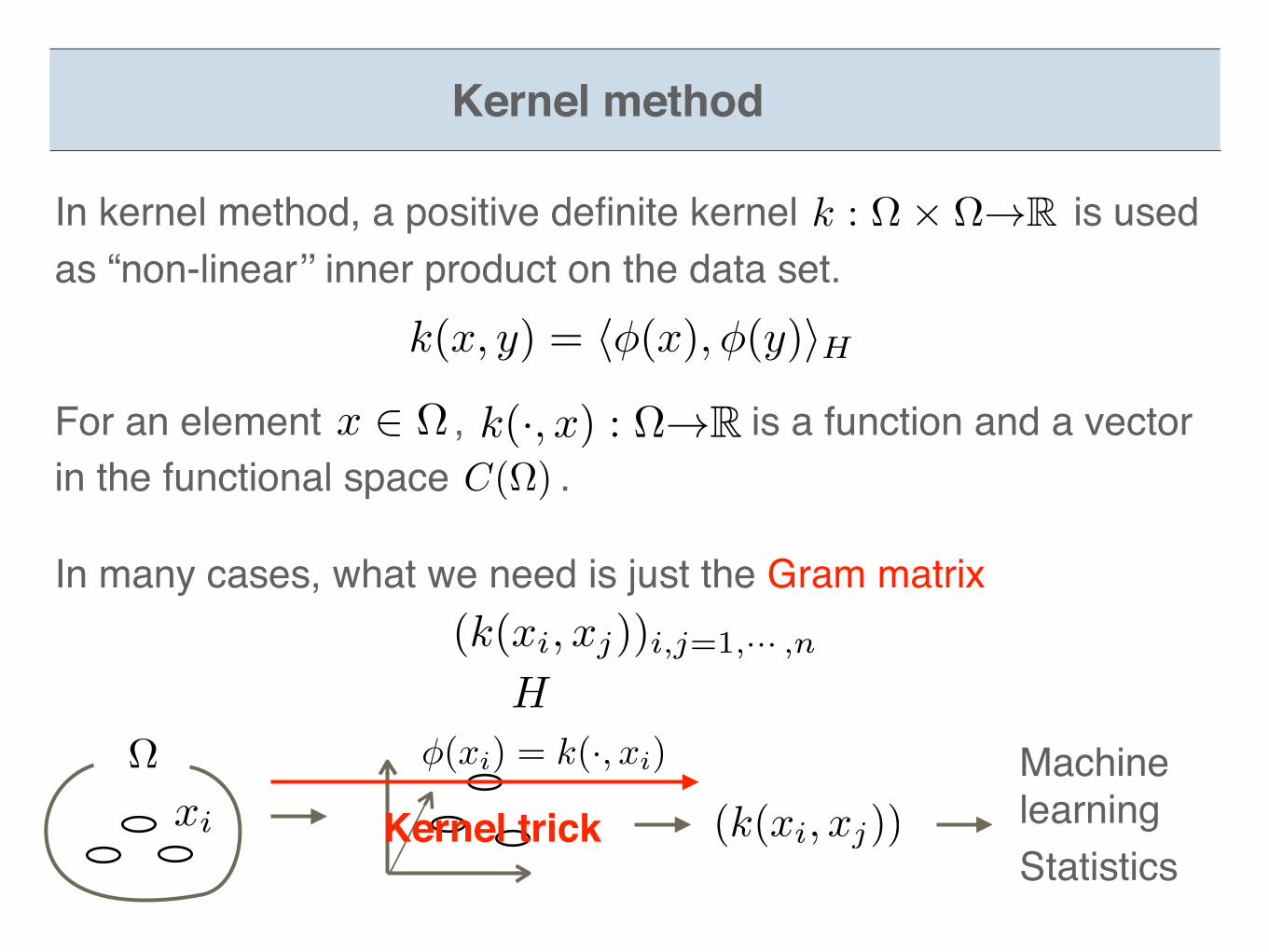
In kernel method, a positive definite kernel is used as “non-linear’’ inner product on the data set.

k : ⌦⇥ ⌦!R

k(x, y) = h�(x),�(y)iH

For an element , is a function and a vector in the functional space .

k(·, x) : ⌦!RC(⌦)

x 2 ⌦

In many cases, what we need is just the Gram matrix(k(xi, xj))i,j=1,··· ,n

Kernel method

⌦

H

(k(xi, xj))

MachinelearningStatistics

xi

�(xi) = k(·, xi)

(k(xi, xj))

MachinelearningStatistics

xi

H

�(xi) = k(·, xi)

Kernel trick

Kernel method

In kernel method, a positive definite kernel is used as “non-linear’’ inner product on the data set.

k : ⌦⇥ ⌦!R

k(x, y) = h�(x),�(y)iH

For an element , is a function and a vector in the functional space .

k(·, x) : ⌦!RC(⌦)

x 2 ⌦

In many cases, what we need is just the Gram matrix(k(xi, xj))i,j=1,··· ,n

⌦

Kernel method

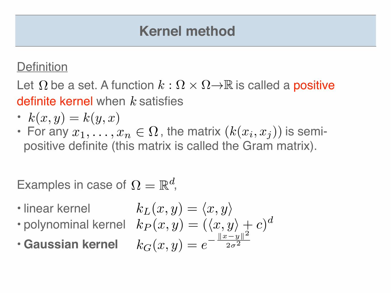
DefinitionLet be a set. A function is called a positive definite kernel when satisfies • • For any , the matrix is semi-

positive definite (this matrix is called the Gram matrix).

k : ⌦⇥ ⌦!R⌦k

k(x, y) = k(y, x)(k(xi, xj))x1, . . . , xn 2 ⌦

Examples in case of ,

• linear kernel• polynominal kernel• Gaussian kernel

⌦ = Rd

kL(x, y) = hx, yikP (x, y) = (hx, yi+ c)d

kG(x, y) = e

� kx�yk2

2�2

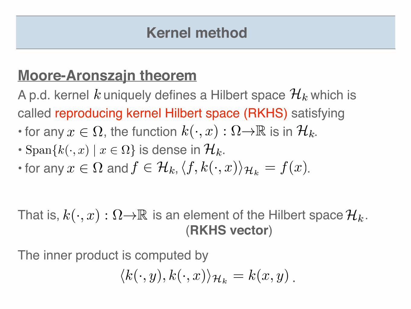
That is, is an element of the Hilbert space . (RKHS vector)

k(·, x) : ⌦!R Hk

The inner product is computed by　　　　　　　　　　　　　　　　　　　.hk(·, y), k(·, x)iHk = k(x, y)

Moore-Aronszajn theoremA p.d. kernel uniquely defines a Hilbert space which is called reproducing kernel Hilbert space (RKHS) satisfying• for any , the function is in . • is dense in . • for any and , .

k Hk

x 2 ⌦ k(·, x) : ⌦!R Hk

Hk

x 2 ⌦ f 2 Hk hf, k(·, x)iHk = f(x)Span{k(·, x) | x 2 ⌦}

Kernel method

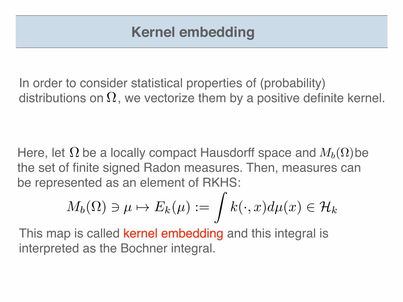
µ 7! Ek(µ) :=

Zk(·, x)dµ(x) 2 HkMb(⌦) 3

Here, let be a locally compact Hausdorff space and be the set of finite signed Radon measures. Then, measures can be represented as an element of RKHS:

Mb(⌦)⌦

This map is called kernel embedding and this integral is interpreted as the Bochner integral.

Kernel embedding

In order to consider statistical properties of (probability) distributions on , we vectorize them by a positive definite kernel.⌦

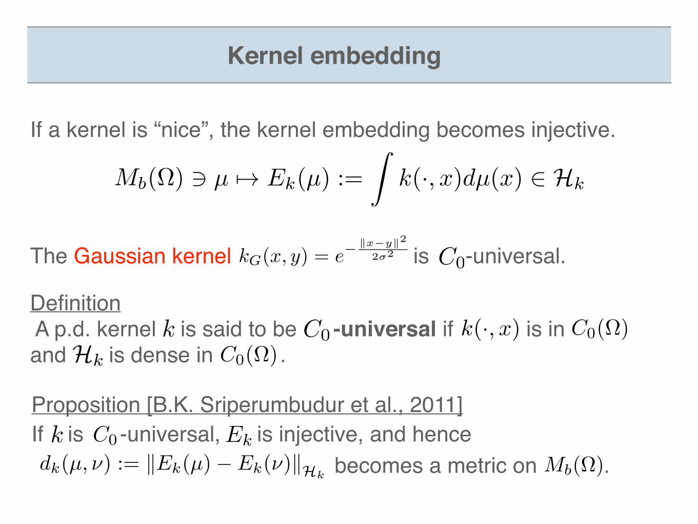
If is -universal, is injective, and hence becomes a metric on .

EkC0kdk(µ, ⌫) := kEk(µ)� Ek(⌫)kHk

Mb(⌦)

Proposition [B.K. Sriperumbudur et al., 2011]

Definition A p.d. kernel is said to be -universal if is in and is dense in .

k C0 C0(⌦)Hk C0(⌦)

k(·, x)

µ 7! Ek(µ) :=

Zk(·, x)dµ(x) 2 HkMb(⌦) 3

If a kernel is “nice”, the kernel embedding becomes injective.

The Gaussian kernel is -universal.kG(x, y) = e

� kx�yk2

2�2 C0

Kernel embedding

Section 3Kernel on persistence diagram

Birth

Death

Birth

Death

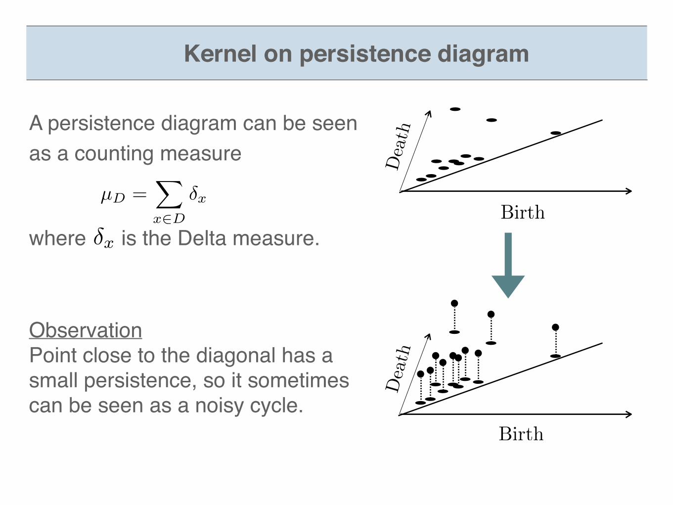
A persistence diagram can be seen as a counting measure

where is the Delta measure.�x

µD

=X

x2D

�x

ObservationPoint close to the diagonal has a small persistence, so it sometimes can be seen as a noisy cycle.

Kernel on persistence diagram

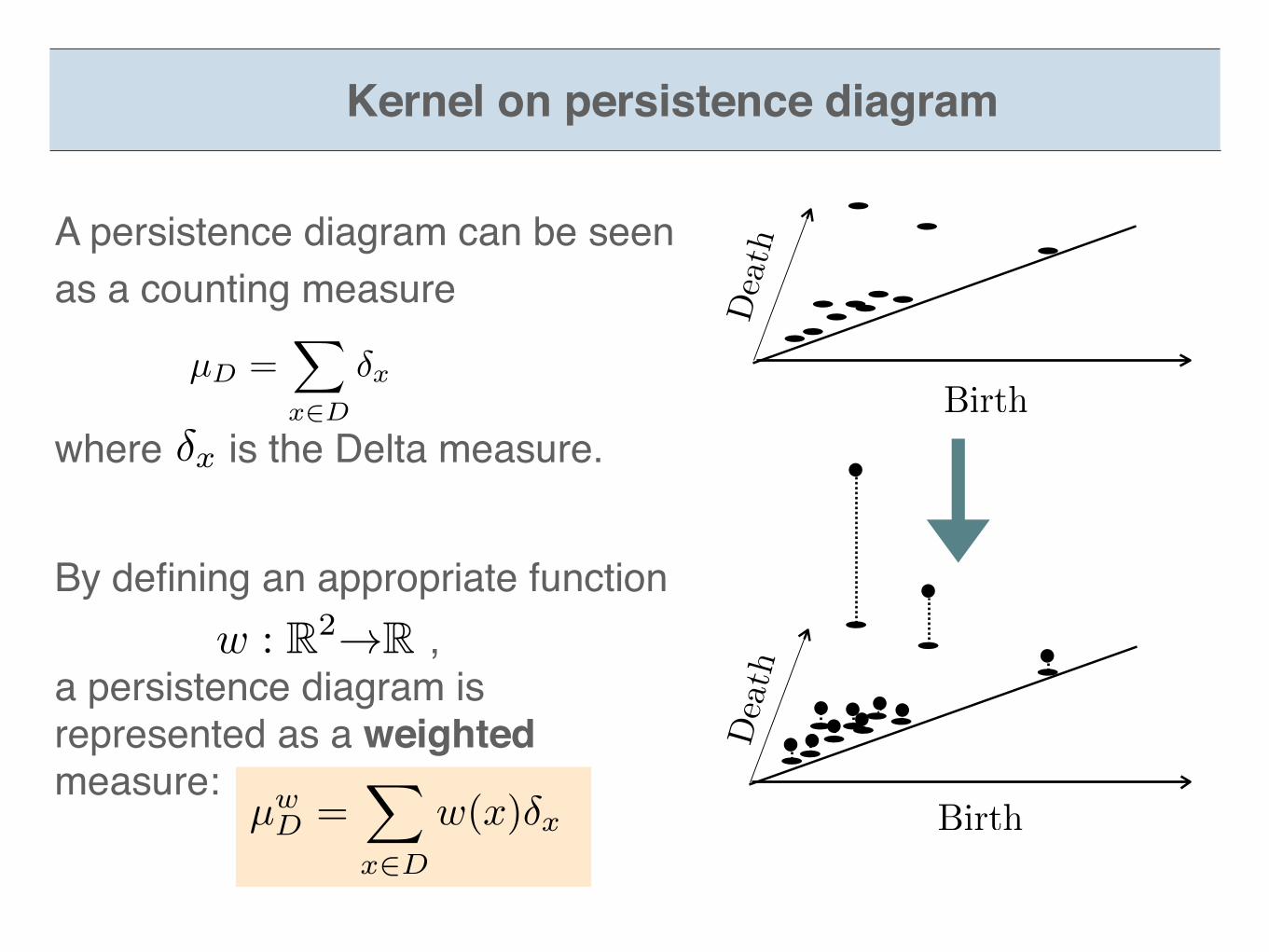
By defining an appropriate function ,a persistence diagram is represented as a weighted measure:

µ

w

D

=X

x2D

w(x)�x

Birth

Death

Birth

Death

w : R2!R

A persistence diagram can be seen as a counting measure

where is the Delta measure.�x

µD

=X

x2D

�x

Kernel on persistence diagram

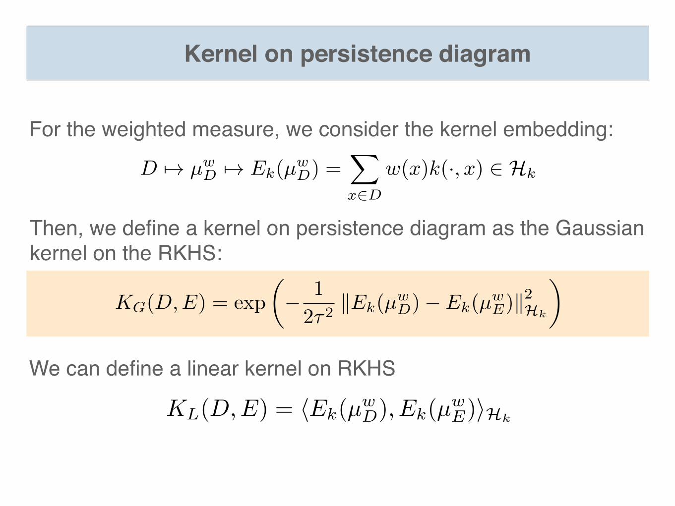
For the weighted measure, we consider the kernel embedding:

D 7! µ

w

D

7! E

k

(µw

D

) =X

x2D

w(x)k(·, x) 2 Hk

Then, we define a kernel on persistence diagram as the Gaussian kernel on the RKHS:

KG(D,E) = exp

✓� 1

2⌧2kEk(µ

wD)� Ek(µ

wE)k

2Hk

◆

We can define a linear kernel on RKHS

KL(D,E) = hEk(µwD), Ek(µ

wE)iHk

Kernel on persistence diagram

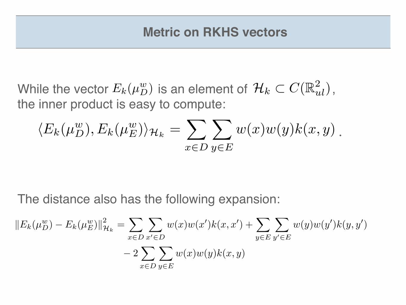
While the vector is an element of ,the inner product is easy to compute:

.

Hk ⇢ C(R2ul)

The distance also has the following expansion:

hEk

(µw

D

), Ek

(µw

E

)iHk =X

x2D

X

y2E

w(x)w(y)k(x, y)

Ek(µwD)

Metric on RKHS vectors

kEk

(µw

D

)� E

k

(µw

E

)k2Hk=

X

x2D

X

x

02D

w(x)w(x0)k(x, x0) +X

y2E

X

y

02E

w(y)w(y0)k(y, y0)

� 2X

x2D

X

y2E

w(x)w(y)k(x, y)

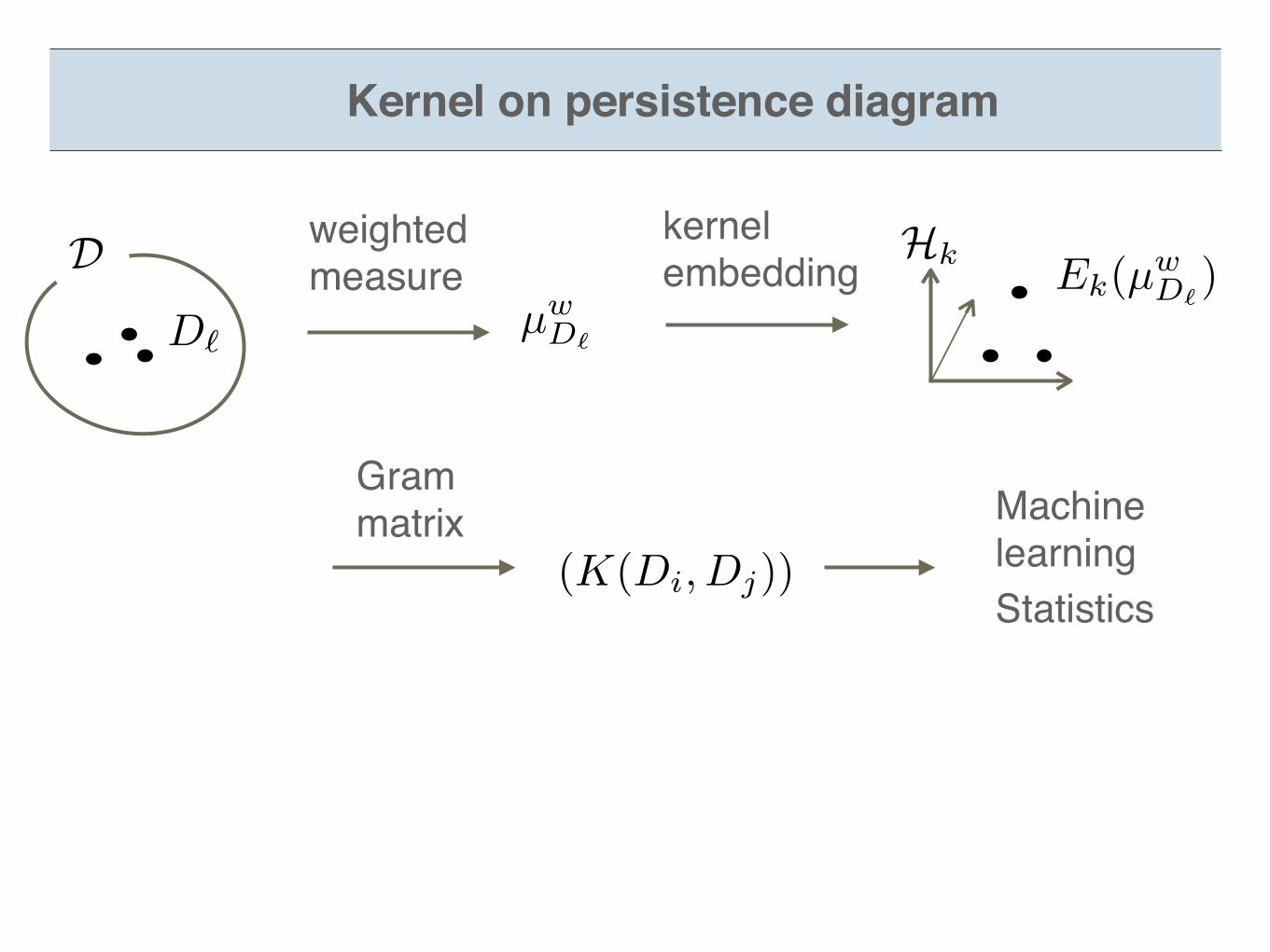
MachinelearningStatistics

D Hk

D`

Ek(µwD`

)

(K(Di, Dj))

µwD`

weighted measure

kernel embedding

Gram matrix

Kernel on persistence diagram

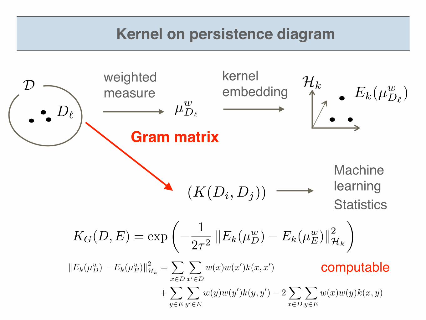
MachinelearningStatistics

(K(Di, Dj))

Gram matrix

KG(D,E) = exp

✓� 1

2⌧2kEk(µ

wD)� Ek(µ

wE)k

2Hk

◆

kEk

(µw

D

)� E

k

(µw

E

)k2Hk=

X

x2D

X

x

02D

w(x)w(x0)k(x, x0)

+X

y2E

X

y

02E

w(y)w(y0)k(y, y0)� 2X

x2D

X

y2E

w(x)w(y)k(x, y)

D Hk

D`

Ek(µwD`

)µwD`

weighted measure

kernel embedding

Kernel on persistence diagram

computable

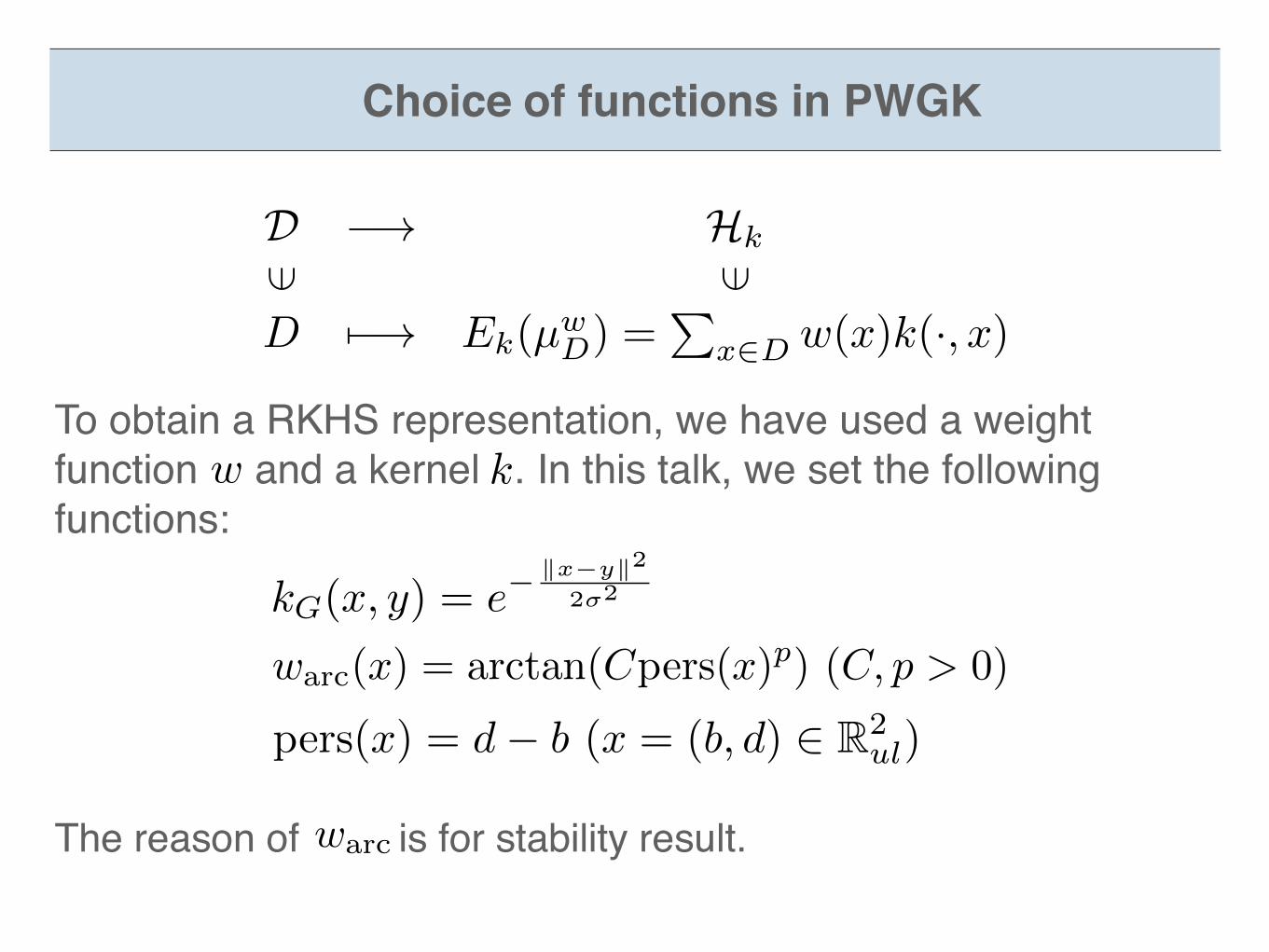
The reason of is for stability result. warc(x) = arctan(Cpers(x)p) (C, p > 0)

pers(x) = d� b (x = (b, d) 2 R2ul)

To obtain a RKHS representation, we have used a weight function and a kernel . In this talk, we set the following functions:

D �! Hk

2 2

D 7�! E

k

(µw

D

) =P

x2D

w(x)k(·, x)

w k

kG(x, y) = e

� kx�yk2

2�2

Choice of functions in PWGK

warc(x) = arctan(Cpers(x)p) (C, p > 0)

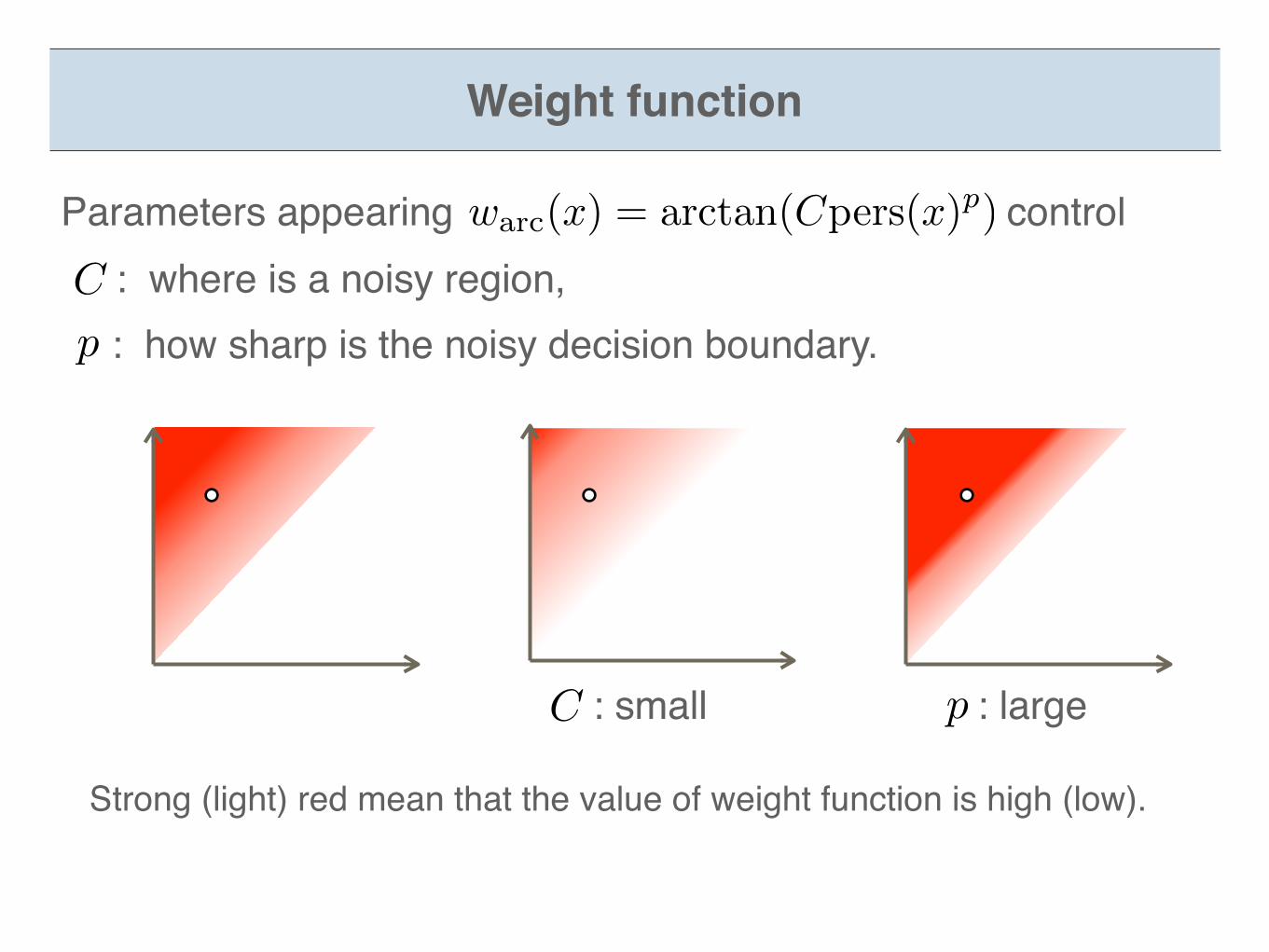
C p: small : large

Weight function

Strong (light) red mean that the value of weight function is high (low).

Parameters appearing 　　　　　　　　　　　　 control : where is a noisy region,　 : how sharp is the noisy decision boundary.p

C

warc(x) = arctan(Cpers(x)p)

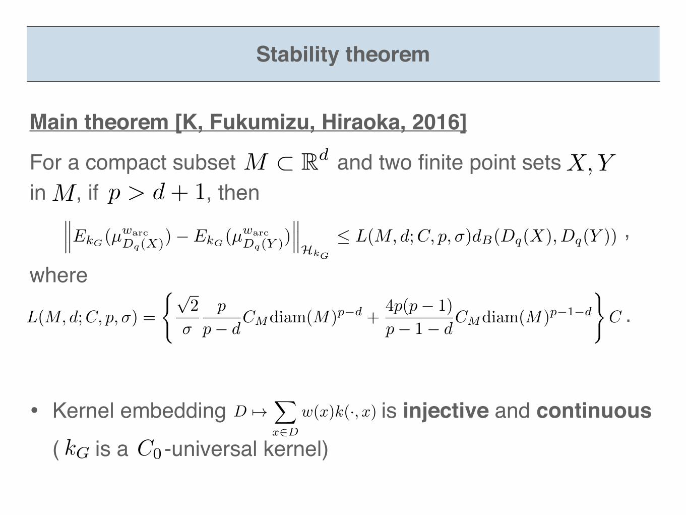
Main theorem [K, Fukumizu, Hiraoka, 2016]

Stability theorem

For a compact subset and two finite point sets in , if , then　　　 ,

where

.

M ⇢ Rd

p > d+ 1

L(M,d;C, p,�) =

(p2

�

p

p� dCMdiam(M)p�d +

4p(p� 1)

p� 1� dCMdiam(M)p�1�d

)C

X,YM���EkG(µ

warc

Dq(X))� EkG(µwarc

Dq(Y ))���HkG

L(M,d;C, p,�)dB(Dq(X), Dq(Y ))

• Kernel embedding is injective and continuous ( is a -universal kernel)

D 7!X

x2D

w(x)k(·, x)

C0kG

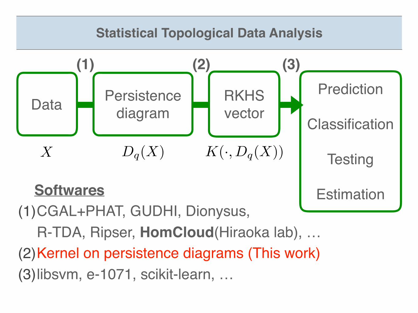
Statistical Topological Data Analysis

DataPrediction

Classification

Testing

Estimation

Persistence diagram

X Dq(X)

RKHSvector

K(·, Dq(X))

(1) (2) (3)

Softwares(1)CGAL+PHAT, GUDHI, Dionysus,

R-TDA, Ripser, HomCloud(Hiraoka lab), …(2)Kernel on persistence diagrams (This work)(3)libsvm, e-1071, scikit-learn, …

Section 4Demonstrations

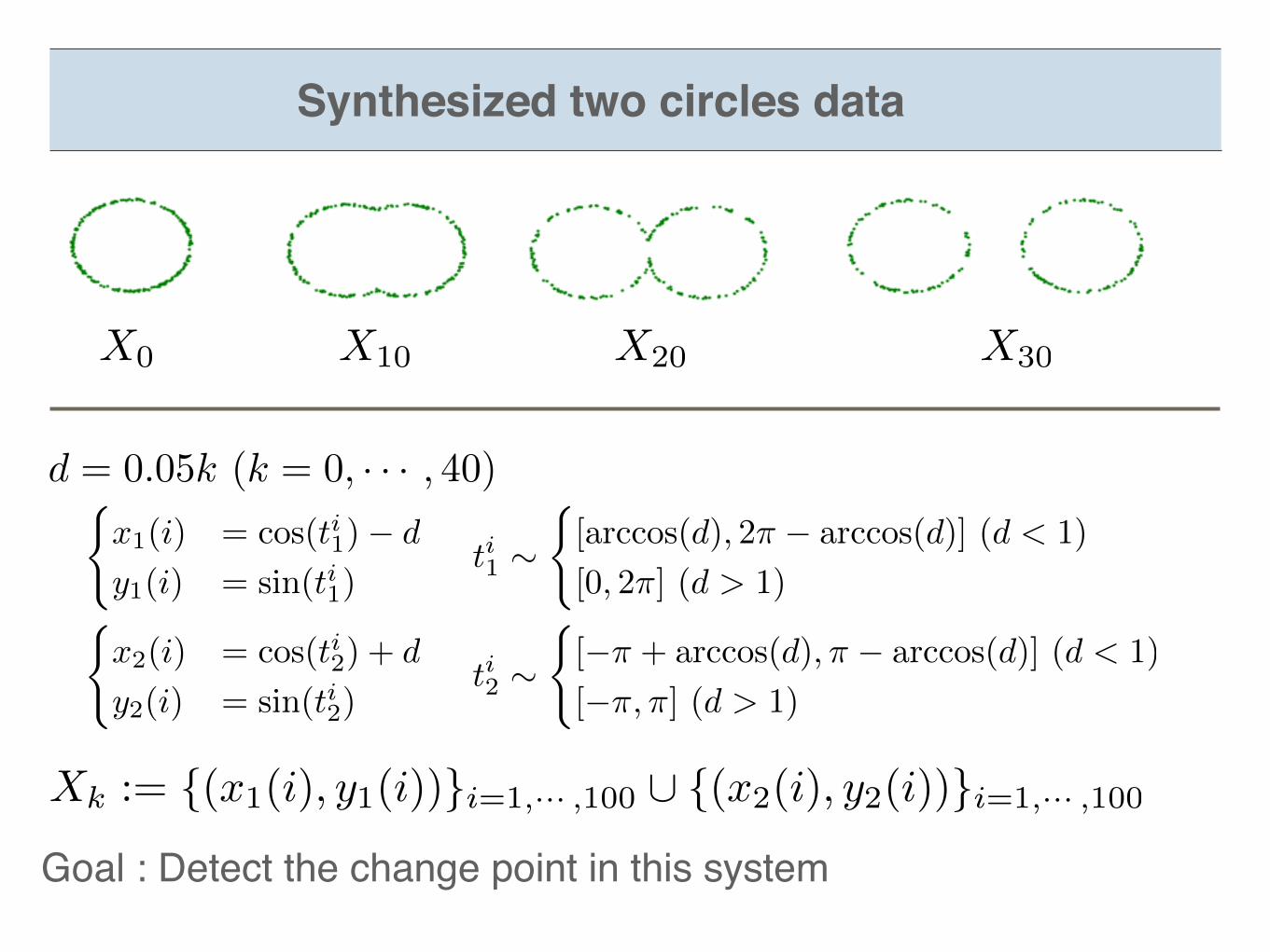
Synthesized two circles data

d = 0.05k (k = 0, · · · , 40)

(x2(i) = cos(t

i2) + d

y2(i) = sin(t

i2)

(x1(i) = cos(t

i1)� d

y1(i) = sin(t

i1)

ti1 ⇠([arccos(d), 2⇡ � arccos(d)] (d < 1)

[0, 2⇡] (d > 1)

ti2 ⇠([�⇡ + arccos(d),⇡ � arccos(d)] (d < 1)

[�⇡,⇡] (d > 1)

Xk := {(x1(i), y1(i))}i=1,··· ,100 [ {(x2(i), y2(i))}i=1,··· ,100

X0 X10 X20 X30

Goal : Detect the change point in this system

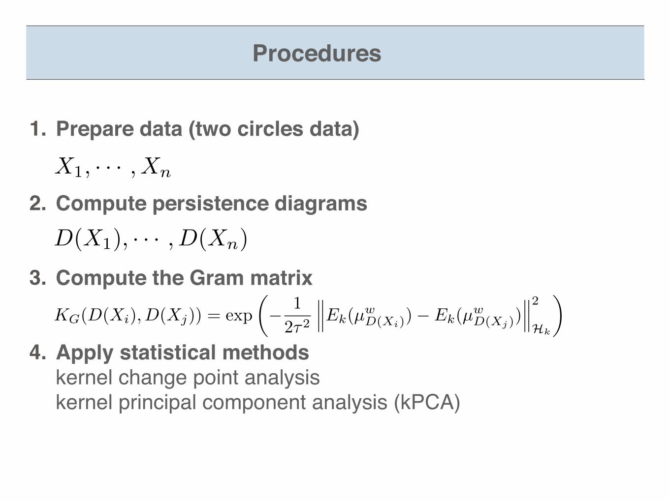
Procedures

1. Prepare data (two circles data)

2. Compute persistence diagrams

3. Compute the Gram matrix

4. Apply statistical methods kernel change point analysiskernel principal component analysis (kPCA)

X1, · · · , Xn

D(X1), · · · , D(Xn)

KG(D(Xi), D(Xj)) = exp

✓� 1

2⌧2

���Ek(µwD(Xi)

)� Ek(µwD(Xj)

)

���2

Hk

◆

Section 5Applications

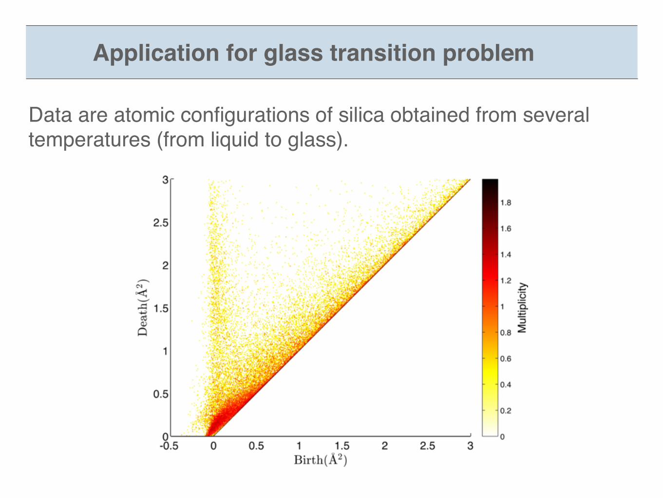
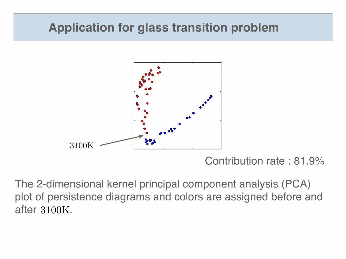
Application for glass transition problem

Data are atomic configurations of silica obtained from several temperatures (from liquid to glass).

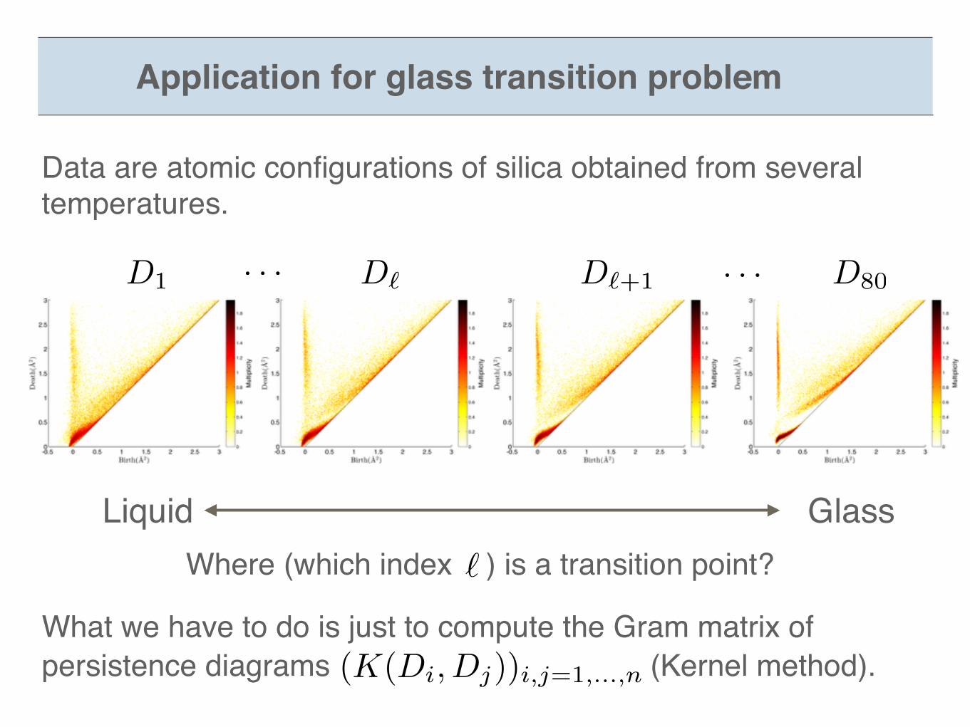
Liquid GlassWhere (which index ) is a transition point?

Application for glass transition problem

D1 D80D` D`+1· · · · · ·

`

Data are atomic configurations of silica obtained from several temperatures.

What we have to do is just to compute the Gram matrix ofpersistence diagrams (Kernel method).(K(Di, Dj))i,j=1,...,n

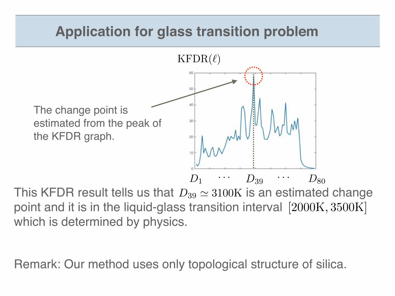
This KFDR result tells us that is an estimated change point and it is in the liquid-glass transition interval which is determined by physics.

The change point is estimated from the peak of the KFDR graph.

D1 D80· · · · · ·

KFDR(`)

[2000K, 3500K]

Remark: Our method uses only topological structure of silica.

Application for glass transition problem

D39 ' 3100KD39

-0.5 0 0.5 1-0.6

-0.4

-0.2

0

0.2

0.4

0.6Glass: KPCA, PWGK

The 2-dimensional kernel principal component analysis (PCA) plot of persistence diagrams and colors are assigned before and after .

Application for glass transition problem

Contribution rate : 81.9%3100K

3100K

Conclusion

Our contribution

Acknowledgment

Reference

Thank you for your attention

: Kernel based statistical framework on persistence diagram

: Takenobu Nakamura (Tohoku University) Ippei Obayashi (Tohoku University) Emerson Escolar (Tohoku University)

G. Kusano, Kenji Fukumizu, and Yasuaki Hiraoka. Persistence weighted Gaussian kernel for topological data analysis, ICML, pp. 2004–2013, 2016.