Embed Size (px)
Citation preview
Statistical Analysis of Repeated Measurements Data
Dimitris RizopoulosDepartment of Biostatistics, Erasmus University Medical Center
@drizopoulos
Contents
1 Motivating Data Sets 1
1.1 Motivating Longitudinal Studies . . . . . . . . . . . . . . . . . . . . . . . . . . 2
1.2 Features of Longitudinal Data . . . . . . . . . . . . . . . . . . . . . . . . . . . 14
1.3 Review of Key Points . . . . . . . . . . . . . . . . . . . . . . . . . . . . . . . 27
2 Marginal Models for Continuous Data 28
2.1 Simple Methods . . . . . . . . . . . . . . . . . . . . . . . . . . . . . . . . . 29
2.2 Review of Linear Regression . . . . . . . . . . . . . . . . . . . . . . . . . . . . 39
2.3 Marginal Models . . . . . . . . . . . . . . . . . . . . . . . . . . . . . . . . . 48
Statistical Analysis of Repeated Measurements Data – D. Rizopoulos ii
2.4 Interpretation . . . . . . . . . . . . . . . . . . . . . . . . . . . . . . . . . . 54
2.5 Estimation . . . . . . . . . . . . . . . . . . . . . . . . . . . . . . . . . . . 72
2.6 Fitting Marginal Models in R . . . . . . . . . . . . . . . . . . . . . . . . . . . 78
2.7 Covariance Matrix . . . . . . . . . . . . . . . . . . . . . . . . . . . . . . . . 82
2.8 Model Building . . . . . . . . . . . . . . . . . . . . . . . . . . . . . . . . . 93
2.9 Hypothesis Testing . . . . . . . . . . . . . . . . . . . . . . . . . . . . . . . . 96
2.10 Confidence Intervals . . . . . . . . . . . . . . . . . . . . . . . . . . . . . . . 120
2.11 Design Considerations - Sample Size . . . . . . . . . . . . . . . . . . . . . . . . 122
2.12 Residuals . . . . . . . . . . . . . . . . . . . . . . . . . . . . . . . . . . . 127
2.13 Review of Key Points . . . . . . . . . . . . . . . . . . . . . . . . . . . . . . 143
Statistical Analysis of Repeated Measurements Data – D. Rizopoulos iii
3 The Linear Mixed Effects Model 145
3.1 The Linear Mixed Model . . . . . . . . . . . . . . . . . . . . . . . . . . . . . 146
3.2 Interpretation . . . . . . . . . . . . . . . . . . . . . . . . . . . . . . . . . . 152
3.3 Hierarchical vs Marginal . . . . . . . . . . . . . . . . . . . . . . . . . . . . . 160
3.4 Estimation . . . . . . . . . . . . . . . . . . . . . . . . . . . . . . . . . . . 170
3.5 Mixed-Effects Models in R . . . . . . . . . . . . . . . . . . . . . . . . . . . . 180
3.6 Nested and Crossed Random Effects∗ . . . . . . . . . . . . . . . . . . . . . . . . 188
3.7 Mixed Models with Correlated Errors . . . . . . . . . . . . . . . . . . . . . . . . 199
3.8 Time-Varying Covariates∗ . . . . . . . . . . . . . . . . . . . . . . . . . . . . . 205
3.9 Model Building . . . . . . . . . . . . . . . . . . . . . . . . . . . . . . . . . 215
3.10 Hypothesis Testing . . . . . . . . . . . . . . . . . . . . . . . . . . . . . . . 218
Statistical Analysis of Repeated Measurements Data – D. Rizopoulos iv
3.11 Residuals . . . . . . . . . . . . . . . . . . . . . . . . . . . . . . . . . . . 241
3.12 Review of Key Points . . . . . . . . . . . . . . . . . . . . . . . . . . . . . . 251
4 Marginal Models for Discrete Data 254
4.1 Review of Generalized Linear Models . . . . . . . . . . . . . . . . . . . . . . . . 255
4.2 Generalized Estimating Equations . . . . . . . . . . . . . . . . . . . . . . . . . 268
4.3 Interpretation . . . . . . . . . . . . . . . . . . . . . . . . . . . . . . . . . . 276
4.4 Generalized Estimating Equations in R . . . . . . . . . . . . . . . . . . . . . . . 283
4.5 Working Correlation Matrix . . . . . . . . . . . . . . . . . . . . . . . . . . . . 286
4.6 Hypothesis Testing . . . . . . . . . . . . . . . . . . . . . . . . . . . . . . . . 297
4.7 Review of Key Points . . . . . . . . . . . . . . . . . . . . . . . . . . . . . . . 306
Statistical Analysis of Repeated Measurements Data – D. Rizopoulos v
5 Mixed Models for Discrete Data 308
5.1 Generalized Linear Mixed Models . . . . . . . . . . . . . . . . . . . . . . . . . . 309
5.2 Interpretation . . . . . . . . . . . . . . . . . . . . . . . . . . . . . . . . . . 316
5.3 Estimation . . . . . . . . . . . . . . . . . . . . . . . . . . . . . . . . . . . 344
5.4 GLMMs in R . . . . . . . . . . . . . . . . . . . . . . . . . . . . . . . . . . 356
5.5 Model Building . . . . . . . . . . . . . . . . . . . . . . . . . . . . . . . . . 361
5.6 Hypothesis Testing . . . . . . . . . . . . . . . . . . . . . . . . . . . . . . . . 363
5.7 Review of Key Points . . . . . . . . . . . . . . . . . . . . . . . . . . . . . . . 368
6 Statistical Analysis with Incomplete Grouped Data 370
6.1 Missing Data in Longitudinal Studies . . . . . . . . . . . . . . . . . . . . . . . . 371
Statistical Analysis of Repeated Measurements Data – D. Rizopoulos vi
6.2 Missing Data Mechanisms . . . . . . . . . . . . . . . . . . . . . . . . . . . . 376
6.3 Analysis with Incomplete Data . . . . . . . . . . . . . . . . . . . . . . . . . . . 391
6.4 Summary . . . . . . . . . . . . . . . . . . . . . . . . . . . . . . . . . . . . 413
6.5 Review of Key Points . . . . . . . . . . . . . . . . . . . . . . . . . . . . . . . 415
7 Closing 417
7.1 Concluding Remarks . . . . . . . . . . . . . . . . . . . . . . . . . . . . . . . 418
7.2 Statistical Analysis Section . . . . . . . . . . . . . . . . . . . . . . . . . . . . 421
Practicals 423
Practical 1: Marginal Models Continuous . . . . . . . . . . . . . . . . . . . . . . . . 424
Practical 2: Mixed Models Continuous . . . . . . . . . . . . . . . . . . . . . . . . . 434
Statistical Analysis of Repeated Measurements Data – D. Rizopoulos vii
Practical 3: Marginal Models Discrete . . . . . . . . . . . . . . . . . . . . . . . . . 443
Practical 4: Mixed Models Discrete . . . . . . . . . . . . . . . . . . . . . . . . . . 451
Statistical Analysis of Repeated Measurements Data – D. Rizopoulos viii

What is this Course About
Grouped data arise in a wide range of disciplines
• Typical examples of grouped data
◃ repeated measurements: measuring the same outcome multiple times on the samesample unit (e.g., biomarkers in patients)
◃ multilevel data: outcomes measured on sample units that are organized indifferent levels (e.g., patients in medical centers or students in schools)
Statistical Analysis of Repeated Measurements Data – D. Rizopoulos ix
What is this Course About (cont’d)
• Statistical analysis of clustered/grouped data
◃ Features of grouped data
◃ describe their distribution
◃ inference using suitable regression models
Statistical Analysis of Repeated Measurements Data – D. Rizopoulos x
Lexical convention
• The following terms are used interchangeably to denote multivariate outcomes
◃ clustered data
◃ repeated measurements data
◃ multilevel data
◃ grouped data
Statistical Analysis of Repeated Measurements Data – D. Rizopoulos xi
Learning Objectives
• Goals: After this course participants will be able to
◃ identify settings in which a repeated measurements model is required,
◃ construct and fit an appropriate model to the data at hand, and
◃ correctly interpret the results
• Even though the course will be primarily explanatory
◃ sufficient mathematical detail will be provided in order participants to obtain aclear view on the different modeling approaches, and how they should be used inpractice
Statistical Analysis of Repeated Measurements Data – D. Rizopoulos xii
Agenda
• Chapter 1: Motivating Data Sets
◃ Data sets that we will use throughout the course
◃ Formulation of possible research questions
◃ Features of repeated measurements data
• Chapter 2: Marginal Models for Continuous Data
◃ Naive approaches
◃ Review linear regression
◃ Marginal models
Statistical Analysis of Repeated Measurements Data – D. Rizopoulos xiii
Agenda (cont’d)
• Chapter 3: The Linear Mixed Effects Model
◃ Mixed effects models
◃ Mixed models with correlated errors
◃ Nested and cross random effects
◃ Time-varying covariates
• Chapter 4: Marginal Models for Discrete Data
◃ Review generalized linear models
◃ Generalized estimating equations
Statistical Analysis of Repeated Measurements Data – D. Rizopoulos xiv
Agenda (cont’d)
• Chapter 5: Mixed Models for Discrete Data
◃ Generalized linear mixed effects models
◃ interpretation of parameters
◃ approximations of the integrand & integral
• Chapter 6: Statistical Analysis with Incomplete Grouped Data
◃ Problems with incomplete data
◃ Missing data mechanisms
◃ Valid inferential approaches
Statistical Analysis of Repeated Measurements Data – D. Rizopoulos xv
Structure of the Course & Material
• Lectures & software practicals using R
• Material:
◃ Course Notes
◃ R code in soft format
• Within the course notes there are several examples of R syntax – these are denotedby the symbol ‘R> ’
Statistical Analysis of Repeated Measurements Data – D. Rizopoulos xvi
Software Requirements
• The up-to-date versions of R and Rstudio; downloadable from
◃ https://cran.r-project.org/
◃ https://www.rstudio.com/
• Additional required packages
◃ nlme, lme4, GLMMadaptive, geepack,
◃ MASS, lattice, shiny, corrplot
Statistical Analysis of Repeated Measurements Data – D. Rizopoulos xvii
Software Requirements
• Up-to-date versions of these packages and their dependencies can be installed usingthe command
install.packages(c("shiny", "nlme", "lattice", "lme4",
"GLMMadaptive", "geepack", "MASS", "corrplot"),
dependencies = TRUE)
• Up-to-date version of a modern web browser, e.g.,
◃ Mozilla Firefox (https://www.mozilla.org/firefox/)
◃ Google Chrome (https://www.google.com/chrome/)
Statistical Analysis of Repeated Measurements Data – D. Rizopoulos xviii
Software Requirements
• We will use a shiny web app that replicates all analyses in the course including alsosome additional illustrations
• The app is available on GitHub and can be invoked using the following two-stepprocedure (assuming internet connection is available and you have installed the aforementioned packages)
1. Start R
2. Run the command
shiny::runGitHub("Repeated_Measurements", "drizopoulos")
this will open a new web browser window (or tab) with the app
• Note: in order the app to be functional you should not close R
Statistical Analysis of Repeated Measurements Data – D. Rizopoulos xix
References
• Some texts in longitudinal data analysis
◃ Demidenko, E. (2004). Mixed Models: Theory and Applications. New York: JohnWiley & Sons.
◃ Diggle, P., Heagerty, P., Liang, K.-Y., and Zeger, S. (2002). Analysis ofLongitudinal Data, 2nd edition. New York: Oxford University Press.
◃ Galecki, A. and Burzykowski, T. (2013). Linear Mixed-Effects Models Using R.New York: Springer-Verlag.
◃ Molenberghs, G. and Verbeke, G. (2005). Models for Discrete Longitudinal Data.New York: Springer-Verlag.
◃ Fitzmaurice, G., Laird, N., and Ware, J. (2011). Applied Longitudinal Analysis,2nd Ed. Hoboken: John Wiley & Sons.
◃ Hand, D. and Crowder, M. (1995). Practical Longitudinal Data Analysis. London:Chapman & Hall.
Statistical Analysis of Repeated Measurements Data – D. Rizopoulos xx
References (cont’d)
• Some texts in longitudinal data analysis
◃ Hedeker, D. and Gibbons, R. (2006). Longitudinal Data Analysis. New York:John Wiley & Sons.
◃ Lindsey, J. (1993). Models for Repeated Measurements. Oxford: OxfordUniversity Press.
◃ Pinheiro, J. and Bates, D. (2000). Mixed Effects Models in S and S-plus. NewYork: Springer-Verlag.
◃ Verbeke, G. and Molenberghs, G. (2000). Linear Mixed Models for LongitudinalData. New York: Springer-Verlag.
Statistical Analysis of Repeated Measurements Data – D. Rizopoulos xxi

Exams
• Written exams
• Scope: Convincingly demonstrate that you have understood the basics of thestatistical analysis of grouped data, and you can apply it on your own
• Format
◃ You will split in groups of 3-4 persons
◃ On the last day of the course you will receive a data set and specific questions
◃ On the exams deadline (see CANVAS) you will need to submit your report onCANVAS – reports submitted after the deadline will NOT be accepted
Statistical Analysis of Repeated Measurements Data – D. Rizopoulos xxii
Disclaimer & Warning!
As you will see, the analysis of repeated measurements data is rathercomplex, and the statistical regression models we have available forthese data cannot be introduced without the use of mathematical
equations
I will try to explain all material simply and intuitively, nevertheless, aweek of equations follows . . .
Statistical Analysis of Repeated Measurements Data – D. Rizopoulos xxiii
Use of Statistical Models
. . . the megalomaniacal strategy of fitting a grand unified model,supposedly capable of answering any conceivable question that might
be posed, is, in our view, dangerous, unnecessary andcounterproductive.
Drum and McCullach (1993, Statistical Science 8, 300–301)
Statistical Analysis of Repeated Measurements Data – D. Rizopoulos xxiv
Chapter 1
Motivating Data Sets
Statistical Analysis of Repeated Measurements Data – D. Rizopoulos 1
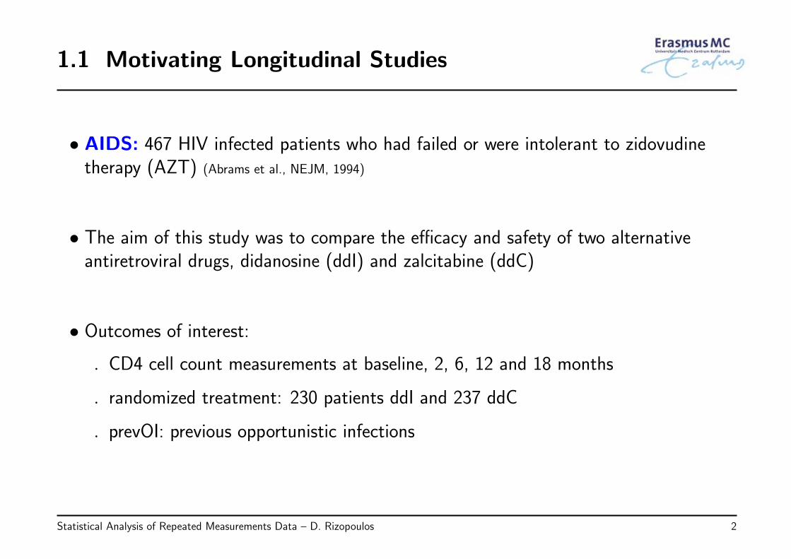
1.1 Motivating Longitudinal Studies
• AIDS: 467 HIV infected patients who had failed or were intolerant to zidovudinetherapy (AZT) (Abrams et al., NEJM, 1994)
• The aim of this study was to compare the efficacy and safety of two alternativeantiretroviral drugs, didanosine (ddI) and zalcitabine (ddC)
• Outcomes of interest:
◃ CD4 cell count measurements at baseline, 2, 6, 12 and 18 months
◃ randomized treatment: 230 patients ddI and 237 ddC
◃ prevOI: previous opportunistic infections
Statistical Analysis of Repeated Measurements Data – D. Rizopoulos 2
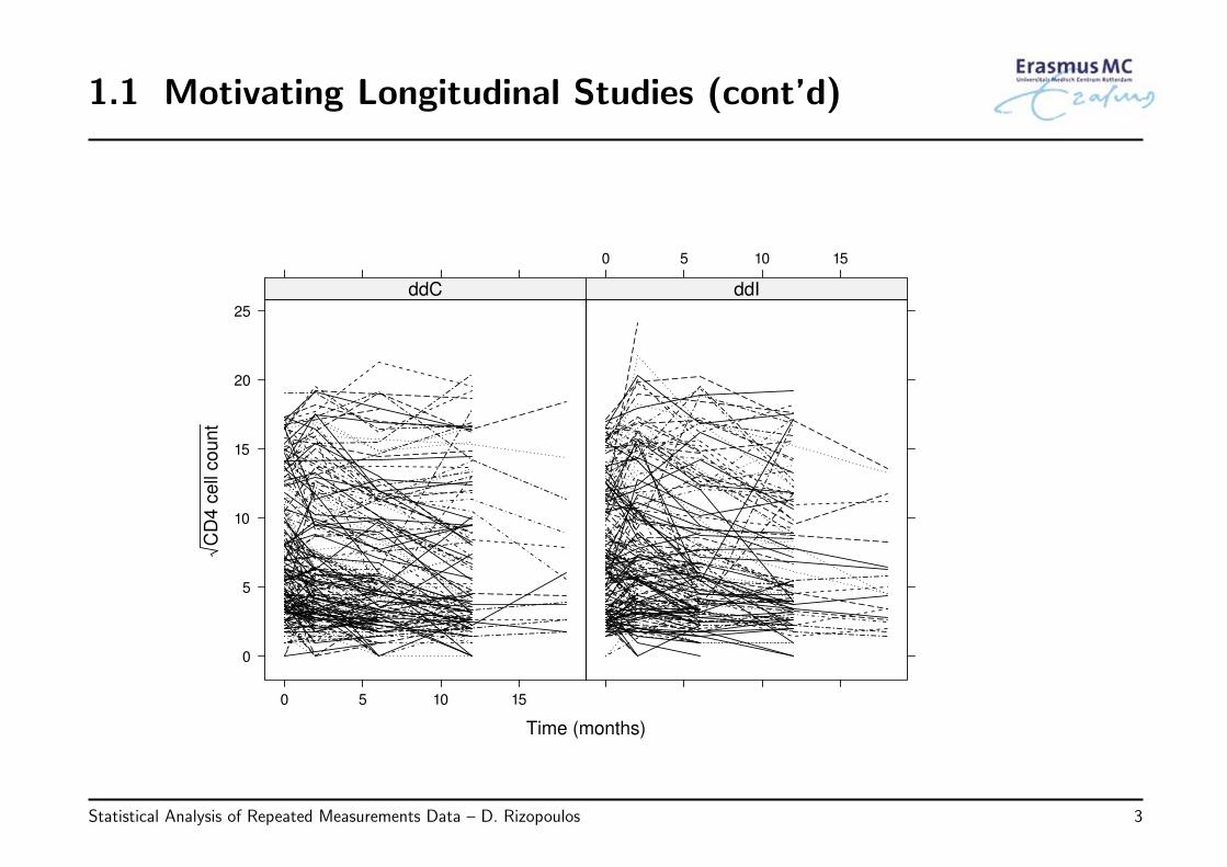
1.1 Motivating Longitudinal Studies (cont’d)
Time (months)
CD
4 c
ell
cou
nt
0
5
10
15
20
25
0 5 10 15
ddC
0 5 10 15
ddI
Statistical Analysis of Repeated Measurements Data – D. Rizopoulos 3
1.1 Motivating Longitudinal Studies (cont’d)
• Research Questions:
◃ How CD4 cell count evolves over time for this cohort of patients?
◃ Does treatment improve average longitudinal evolutions?
Statistical Analysis of Repeated Measurements Data – D. Rizopoulos 4

1.1 Motivating Longitudinal Studies (cont’d)
• PBC: Primary Biliary Cirrhosis:
◃ a chronic, fatal but rare liver disease
◃ characterized by inflammatory destruction of the small bile ducts within the liver
• Data collected by Mayo Clinic from 1974 to 1984 (Murtaugh et al., Hepatology, 1994)
• Outcomes of interest:
◃ longitudinal serum bilirubin, serum cholesterol, prothrombin time
◃ randomized treatment: 158 patients received D-penicillamine and 154 placebo
Statistical Analysis of Repeated Measurements Data – D. Rizopoulos 5
1.1 Motivating Longitudinal Studies (cont’d)
Time (years)
log
(se
rum
Bili
rub
in (
mg
/dL)) −1
0123
38
0 5 10
39 51
0 5 10
68
70 82 90
−10123
93
−10123
134 148 173 200
0 5 10
216 242
0 5 10
269
−10123
290
Statistical Analysis of Repeated Measurements Data – D. Rizopoulos 6
1.1 Motivating Longitudinal Studies (cont’d)
• Research Questions:
◃ Do men have higher serum bilirubin during follow-up than women?
◃ Is there a difference in the average longitudinal evolutions of serum bilirubinbetween the two treatments when we correct for age and gender at baseline?
Statistical Analysis of Repeated Measurements Data – D. Rizopoulos 7

1.1 Motivating Longitudinal Studies (cont’d)
• Prothro: Prednisone versus placebo in liver cirrhosis patients
◃ slowly progressing disease in which healthy liver tissue is replaced with scar tissue,eventually preventing the liver from functioning properly
• Randomized trial in Denmark (Andersen et al., Springer, 1993)
• Outcomes of interest:
◃ randomized treatment: 237 patients received prednisone and 251 placebo
◃ longitudinal prothrombin times
Statistical Analysis of Repeated Measurements Data – D. Rizopoulos 8
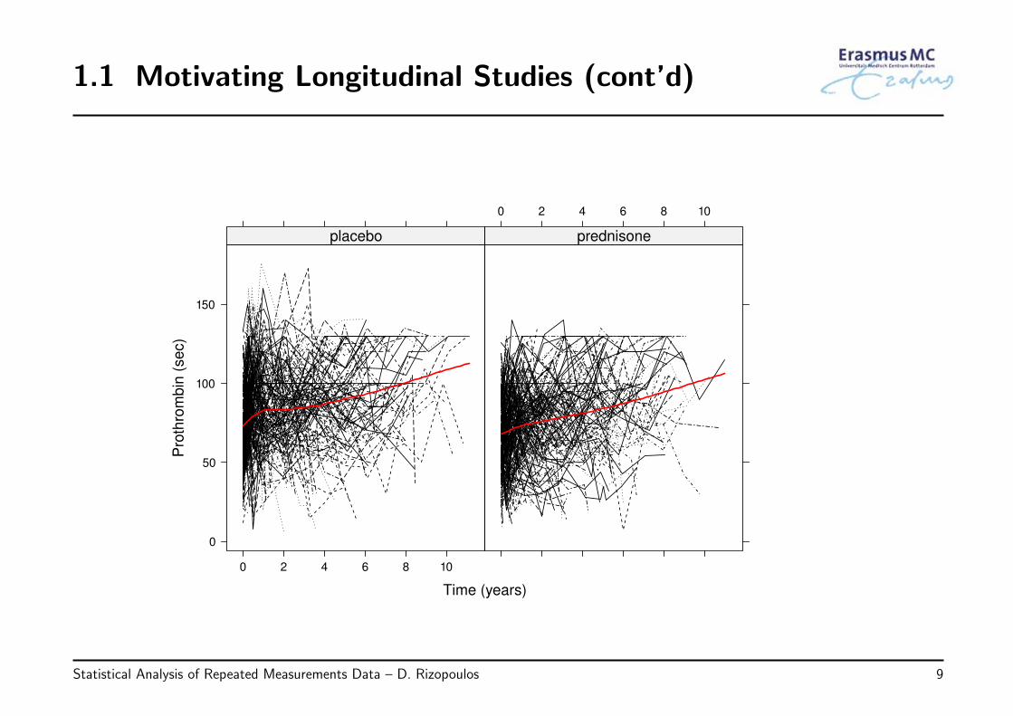
1.1 Motivating Longitudinal Studies (cont’d)
Time (years)
Pro
thro
mb
in (
se
c)
0
50
100
150
0 2 4 6 8 10
placebo
0 2 4 6 8 10
prednisone
Statistical Analysis of Repeated Measurements Data – D. Rizopoulos 9

1.1 Motivating Longitudinal Studies (cont’d)
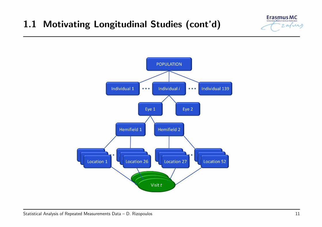
• Glaucoma: A group of eye conditions resulting in optic nerve damage, which maycause loss of vision
• Ongoing prospective cohort study on 139 patients (80% men) conducted by theRotterdam Eye Hospital in the Netherlands http://rod-rep.com
• Outcome of interest:
◃ Visual field (VF) sensitivity collected at approximately 6-months intervals
Statistical Analysis of Repeated Measurements Data – D. Rizopoulos 10
1.1 Motivating Longitudinal Studies (cont’d)
Statistical Analysis of Repeated Measurements Data – D. Rizopoulos 11
1.1 Motivating Longitudinal Studies (cont’d)
Time (years)
Sensitiv
ity E
stim
ate
(dB
)0 2 4 6 8 10 0 2 4 6 8 10
51015202530
51015202530
51015202530
0 2 4 6 8 10 0 2 4 6 8 10
51015202530
Statistical Analysis of Repeated Measurements Data – D. Rizopoulos 12
1.1 Motivating Longitudinal Studies (cont’d)
• Research Questions:
◃ Study disease progression using VF sensitivity
◃ Predict rate of progression for future patients
Statistical Analysis of Repeated Measurements Data – D. Rizopoulos 13
1.2 Features of Longitudinal Data
• Repeated evaluations of the same outcome in each subject over time
◃ CD4 cell count in HIV-infected patients
◃ serum bilirubin in PBC patients
• Visiting process
◃ some times fixed by design (e.g., in randomized trials) but often not everybodyadheres to them
◃ completely determined by the physicians and/or the patients
Statistical Analysis of Repeated Measurements Data – D. Rizopoulos 14
1.2 Features of Longitudinal Data (cont’d)
Measurements on the same subject are expected tobe (positively) correlated
• This implies that standard statistical tools, such as the t-test and simple linearregression that assume independent observations, are not optimal for longitudinaldata analysis
Statistical Analysis of Repeated Measurements Data – D. Rizopoulos 15
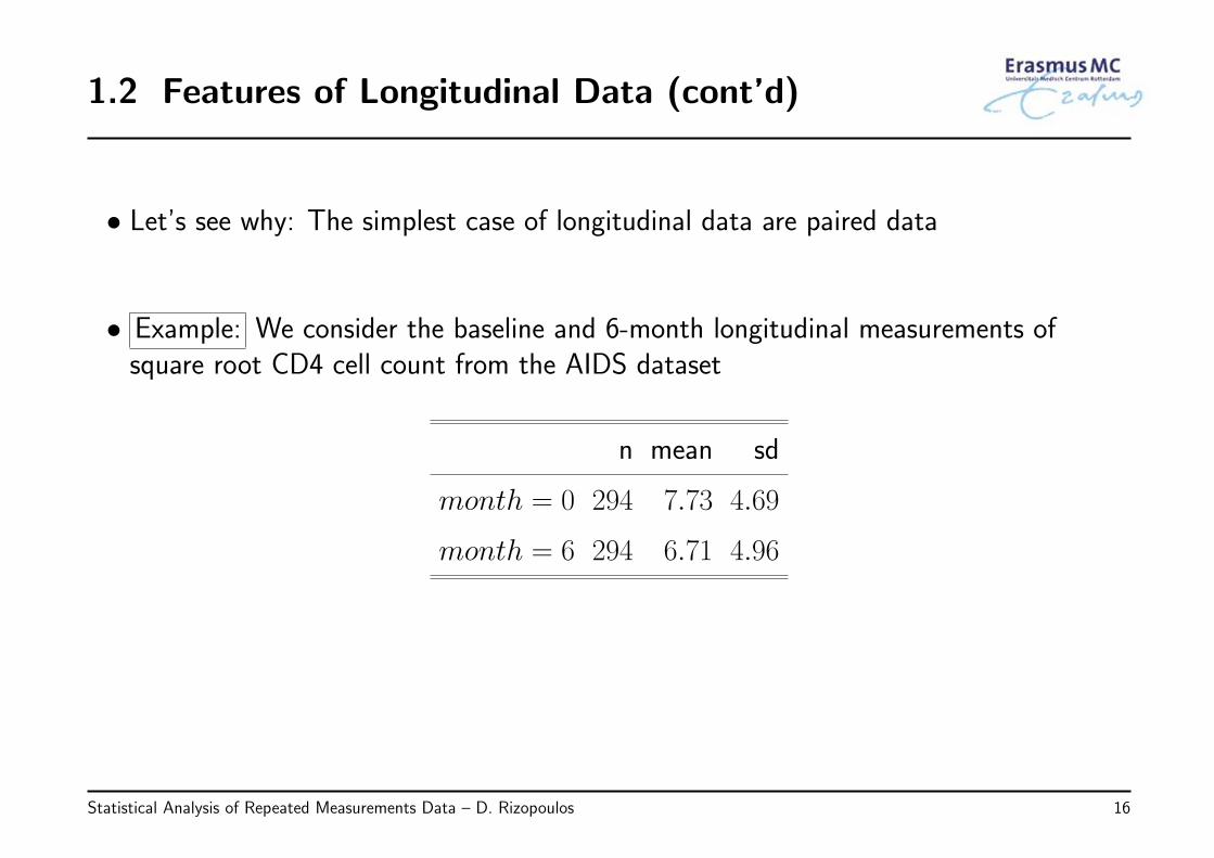
1.2 Features of Longitudinal Data (cont’d)
• Let’s see why: The simplest case of longitudinal data are paired data
• Example: We consider the baseline and 6-month longitudinal measurements ofsquare root CD4 cell count from the AIDS dataset
n mean sd
month = 0 294 7.73 4.69
month = 6 294 6.71 4.96
Statistical Analysis of Repeated Measurements Data – D. Rizopoulos 16
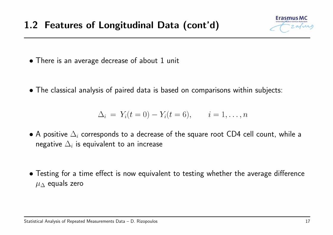
1.2 Features of Longitudinal Data (cont’d)
• There is an average decrease of about 1 unit
• The classical analysis of paired data is based on comparisons within subjects:
∆i = Yi(t = 0)− Yi(t = 6), i = 1, . . . , n
• A positive ∆i corresponds to a decrease of the square root CD4 cell count, while anegative ∆i is equivalent to an increase
• Testing for a time effect is now equivalent to testing whether the average differenceµ∆ equals zero
Statistical Analysis of Repeated Measurements Data – D. Rizopoulos 17
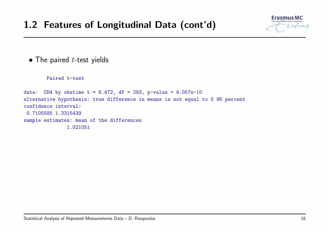
1.2 Features of Longitudinal Data (cont’d)
• The paired t-test yields
Paired t-test
data: CD4 by obstime t = 6.472, df = 293, p-value = 4.057e-10
alternative hypothesis: true difference in means is not equal to 0 95 percent
confidence interval:
0.7105585 1.3315439
sample estimates: mean of the differences
1.021051
Statistical Analysis of Repeated Measurements Data – D. Rizopoulos 18
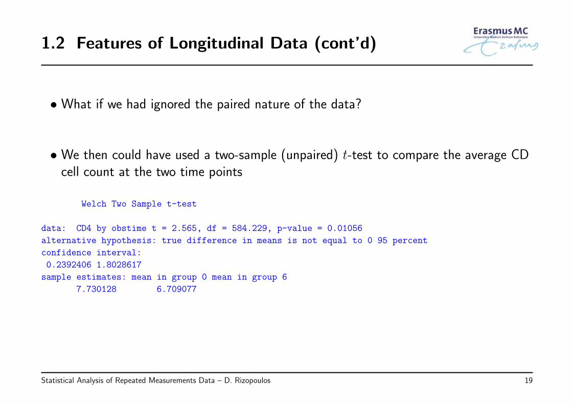
1.2 Features of Longitudinal Data (cont’d)
• What if we had ignored the paired nature of the data?
• We then could have used a two-sample (unpaired) t-test to compare the average CDcell count at the two time points
Welch Two Sample t-test
data: CD4 by obstime t = 2.565, df = 584.229, p-value = 0.01056
alternative hypothesis: true difference in means is not equal to 0 95 percent
confidence interval:
0.2392406 1.8028617
sample estimates: mean in group 0 mean in group 6
7.730128 6.709077
Statistical Analysis of Repeated Measurements Data – D. Rizopoulos 19
1.2 Features of Longitudinal Data (cont’d)
• We would still have found a significant difference (p = 0.0106), but the p-valuewould have been several orders of the magnitude larger than the one obtained fromthe paired t-test
• The two-sample t-test does not take into account that the measurements are notindependent
◃ p-values wrongly too small for between subjects effects
◃ p-values wrongly too large for within subjects effects
• The different effects
◃ between subjects: examine differences between subjects (e.g., males vs females)
◃ within subjects: examine how much subjects tend to change over time
Statistical Analysis of Repeated Measurements Data – D. Rizopoulos 20
1.2 Features of Longitudinal Data (cont’d)
• This illustrates that classical statistical models which assume independentobservations will not be optimal for the analysis of clustered data
Statistical Analysis of Repeated Measurements Data – D. Rizopoulos 21
1.2 Features of Longitudinal Data (cont’d)
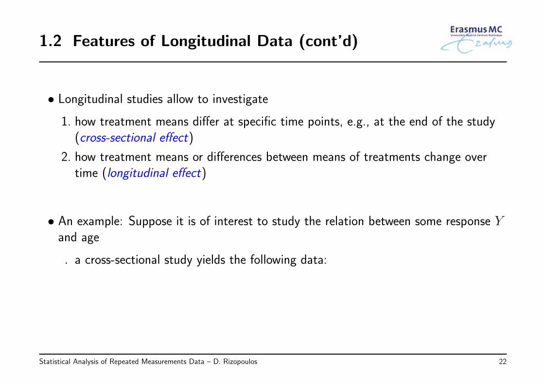
• Longitudinal studies allow to investigate
1. how treatment means differ at specific time points, e.g., at the end of the study(cross-sectional effect)
2. how treatment means or differences between means of treatments change overtime (longitudinal effect)
• An example: Suppose it is of interest to study the relation between some response Yand age
◃ a cross-sectional study yields the following data:
Statistical Analysis of Repeated Measurements Data – D. Rizopoulos 22
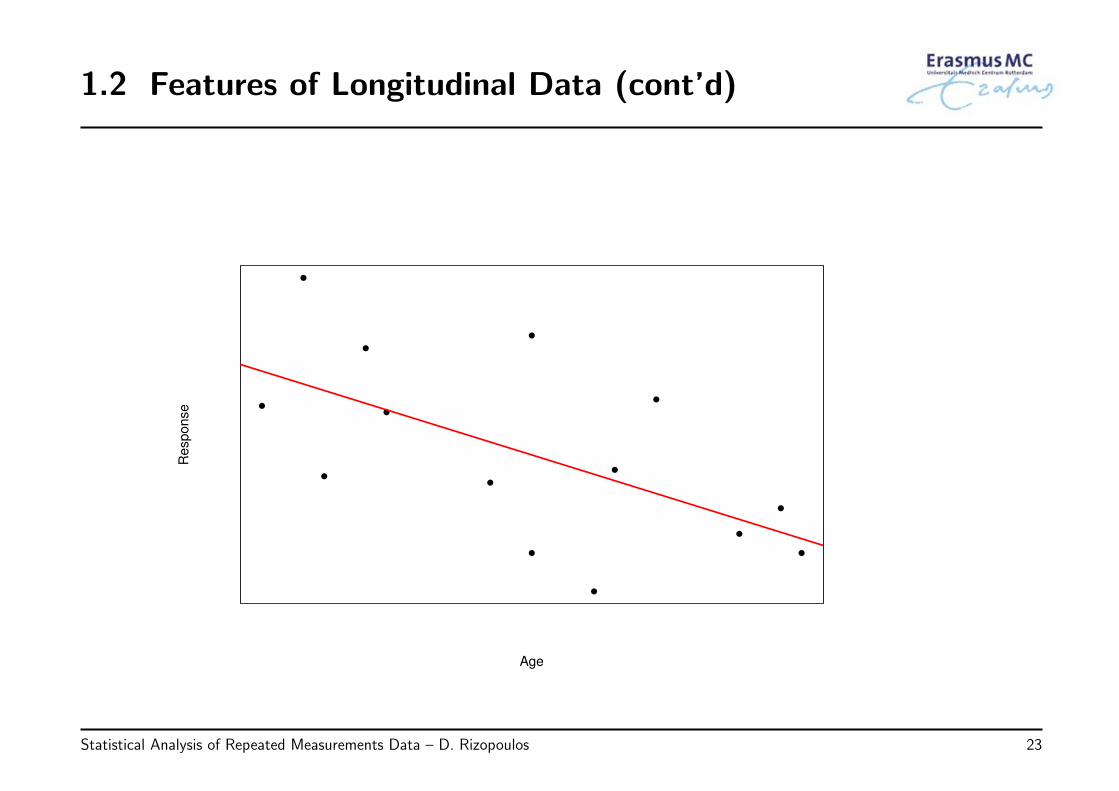
1.2 Features of Longitudinal Data (cont’d)
Age
Re
sp
on
se
Statistical Analysis of Repeated Measurements Data – D. Rizopoulos 23
1.2 Features of Longitudinal Data (cont’d)
• The graph clearly suggests a negative relation between Y and age
• Nevertheless, exactly the same observations also could have been obtained in alongitudinal study, with 2 measurements per subject
Statistical Analysis of Repeated Measurements Data – D. Rizopoulos 24
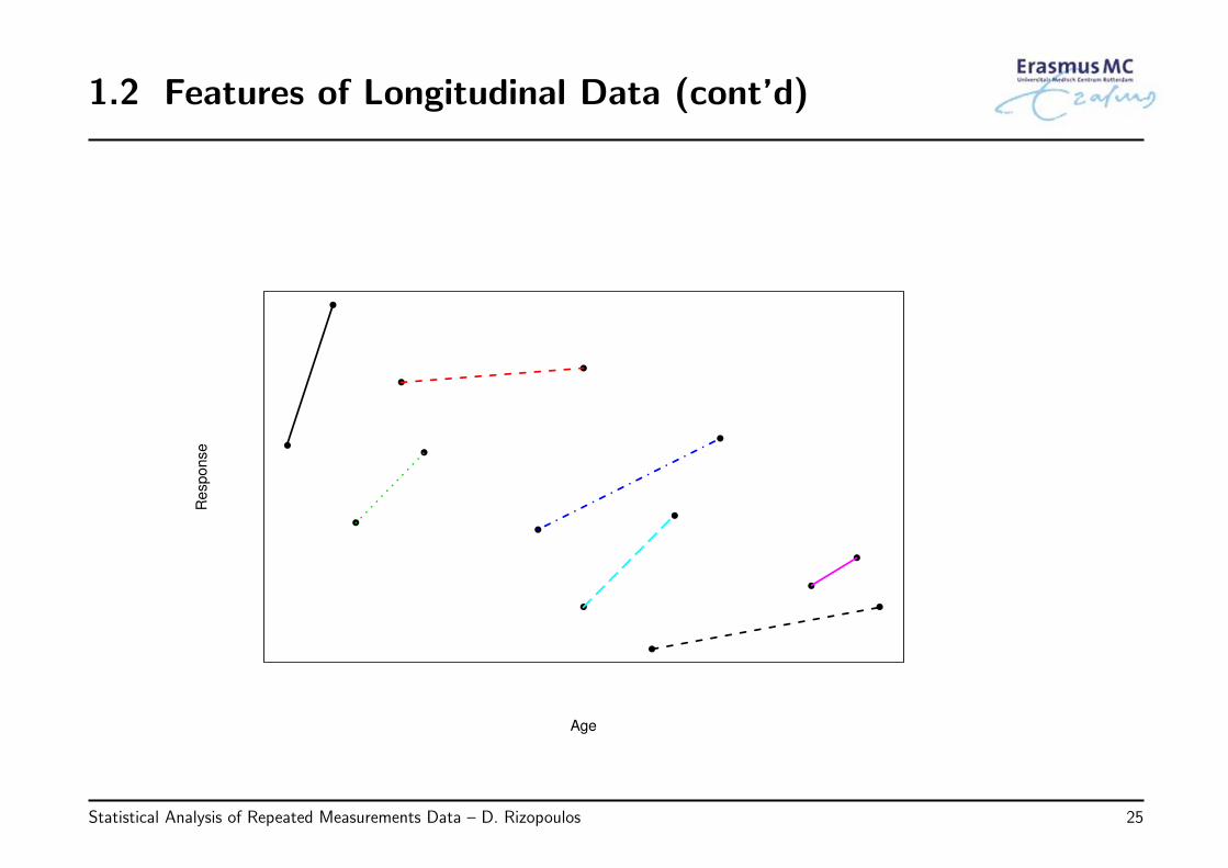
1.2 Features of Longitudinal Data (cont’d)
Age
Re
sp
on
se
Statistical Analysis of Repeated Measurements Data – D. Rizopoulos 25
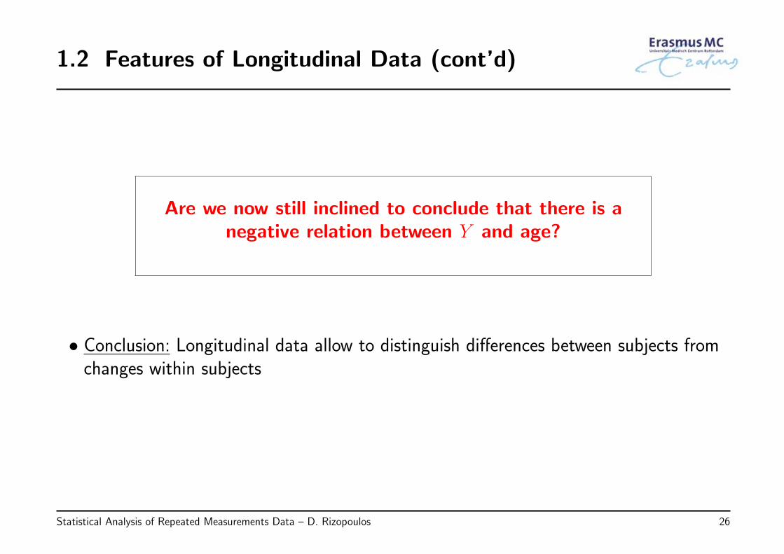
1.2 Features of Longitudinal Data (cont’d)
Are we now still inclined to conclude that there is anegative relation between Y and age?
• Conclusion: Longitudinal data allow to distinguish differences between subjects fromchanges within subjects
Statistical Analysis of Repeated Measurements Data – D. Rizopoulos 26
1.3 Review of Key Points
• Grouped & longitudinal data: Features
◃ measurements on the same subject are correlated
◃ allow to distinguish within and between subjects effects
Statistical Analysis of Repeated Measurements Data – D. Rizopoulos 27
Chapter 2
Marginal Models for Continuous Data
Statistical Analysis of Repeated Measurements Data – D. Rizopoulos 28
2.1 Simple Methods
• The reason why classical statistical techniques fail in the context of longitudinal datais that observations within subjects are correlated
◃ often the correlation between two repeated measurements decreases as the timespan between those measurements increases
• The paired t-test accounts for this by considering subject-specific differences∆i = Yi1 − Yi2
◃ this reduces the number of measurements to just one per subject, which impliesthat classical techniques can be applied again
Statistical Analysis of Repeated Measurements Data – D. Rizopoulos 29
2.1 Simple Methods (cont’d)
• In the case of more than 2 measurements per subject, similar simple techniques areoften applied to reduce the number of measurements for the i-th subject, from ni to 1
◃ Analysis at each time point separately
◃ Analysis of Area Under the Curve (AUC)
◃ Analysis of endpoints
◃ Analysis of increments
Statistical Analysis of Repeated Measurements Data – D. Rizopoulos 30
2.1 Simple Methods (cont’d)
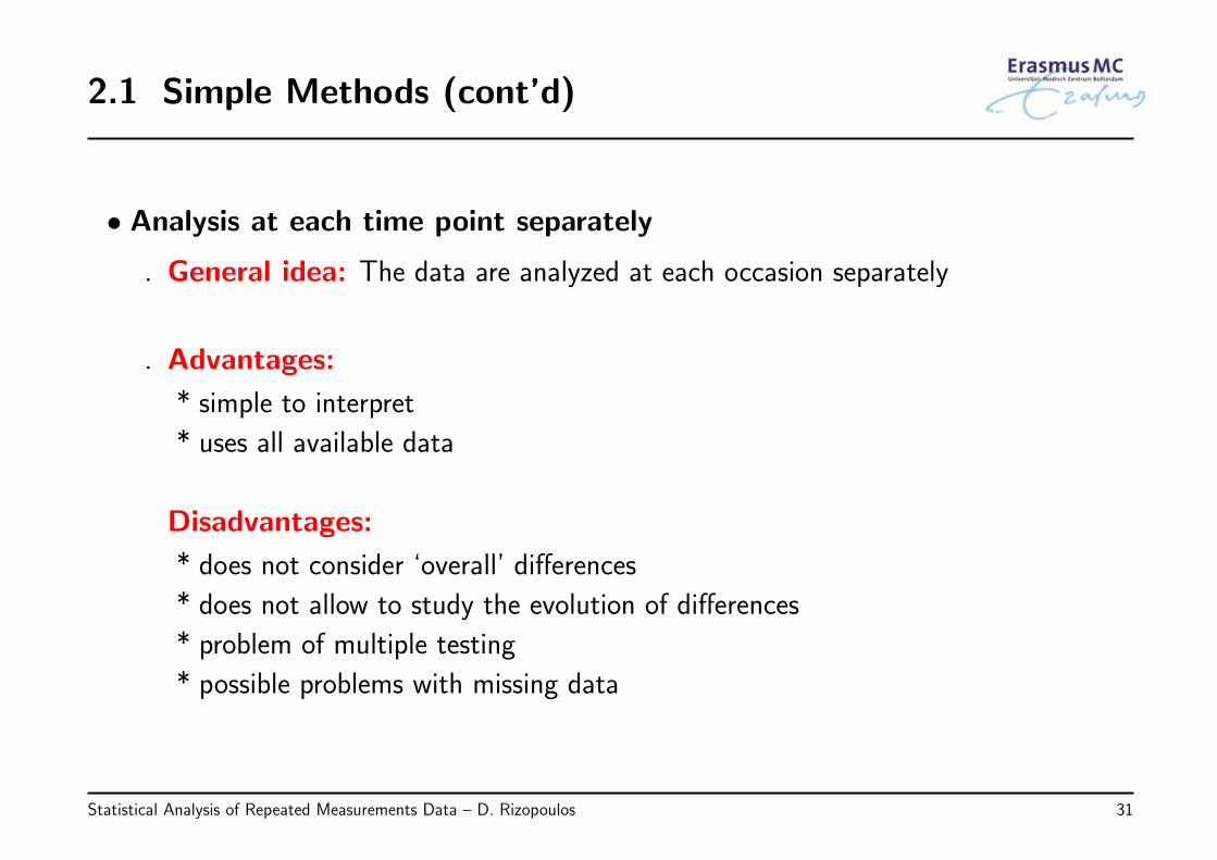
• Analysis at each time point separately
◃ General idea: The data are analyzed at each occasion separately
◃ Advantages:
* simple to interpret
* uses all available data
Disadvantages:
* does not consider ‘overall’ differences
* does not allow to study the evolution of differences
* problem of multiple testing
* possible problems with missing data
Statistical Analysis of Repeated Measurements Data – D. Rizopoulos 31
2.1 Simple Methods (cont’d)
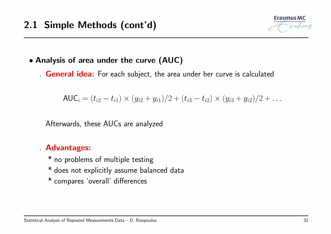
• Analysis of area under the curve (AUC)
◃ General idea: For each subject, the area under her curve is calculated
AUCi = (ti2 − ti1)× (yi2 + yi1)/2 + (ti3 − ti2)× (yi3 + yi2)/2 + . . .
Afterwards, these AUCs are analyzed
◃ Advantages:
* no problems of multiple testing
* does not explicitly assume balanced data
* compares ‘overall’ differences
Statistical Analysis of Repeated Measurements Data – D. Rizopoulos 32
2.1 Simple Methods (cont’d)
• Analysis of area under the curve (AUC)
◃ Disadvantages:
* subjects could have the same AUC but completely different profiles
* possible problems with missing data
Statistical Analysis of Repeated Measurements Data – D. Rizopoulos 33
2.1 Simple Methods (cont’d)
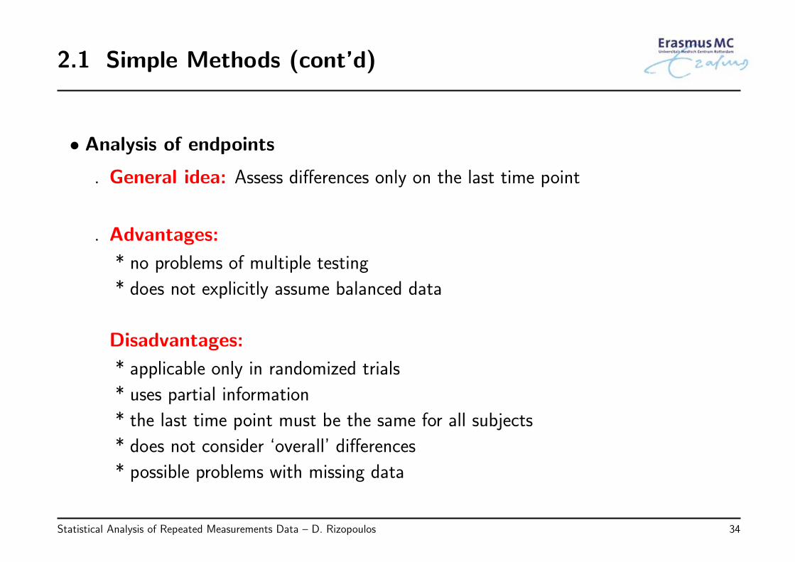
• Analysis of endpoints
◃ General idea: Assess differences only on the last time point
◃ Advantages:
* no problems of multiple testing
* does not explicitly assume balanced data
Disadvantages:
* applicable only in randomized trials
* uses partial information
* the last time point must be the same for all subjects
* does not consider ‘overall’ differences
* possible problems with missing data
Statistical Analysis of Repeated Measurements Data – D. Rizopoulos 34
2.1 Simple Methods (cont’d)
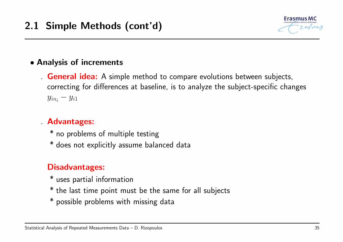
• Analysis of increments
◃ General idea: A simple method to compare evolutions between subjects,correcting for differences at baseline, is to analyze the subject-specific changesyini − yi1
◃ Advantages:
* no problems of multiple testing
* does not explicitly assume balanced data
Disadvantages:
* uses partial information
* the last time point must be the same for all subjects
* possible problems with missing data
Statistical Analysis of Repeated Measurements Data – D. Rizopoulos 35
2.1 Simple Methods (cont’d)
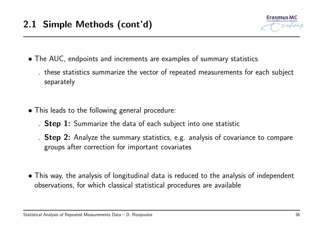
• The AUC, endpoints and increments are examples of summary statistics
◃ these statistics summarize the vector of repeated measurements for each subjectseparately
• This leads to the following general procedure:
◃ Step 1: Summarize the data of each subject into one statistic
◃ Step 2: Analyze the summary statistics, e.g. analysis of covariance to comparegroups after correction for important covariates
• This way, the analysis of longitudinal data is reduced to the analysis of independentobservations, for which classical statistical procedures are available
Statistical Analysis of Repeated Measurements Data – D. Rizopoulos 36
2.1 Simple Methods (cont’d)
• However, all these methods have the disadvantage that (lots of) information is lost
This has led to the development of statisticaltechniques that overcome these disadvantages
Statistical Analysis of Repeated Measurements Data – D. Rizopoulos 37
2.1 Simple Methods (cont’d)
• These techniques are based on extensions of simple regression models for univariatedata
• Before introducing these extensions we start with a short review of the classical linearregression model for continuous outcomes. . .
Statistical Analysis of Repeated Measurements Data – D. Rizopoulos 38
2.2 Review of Linear Regression
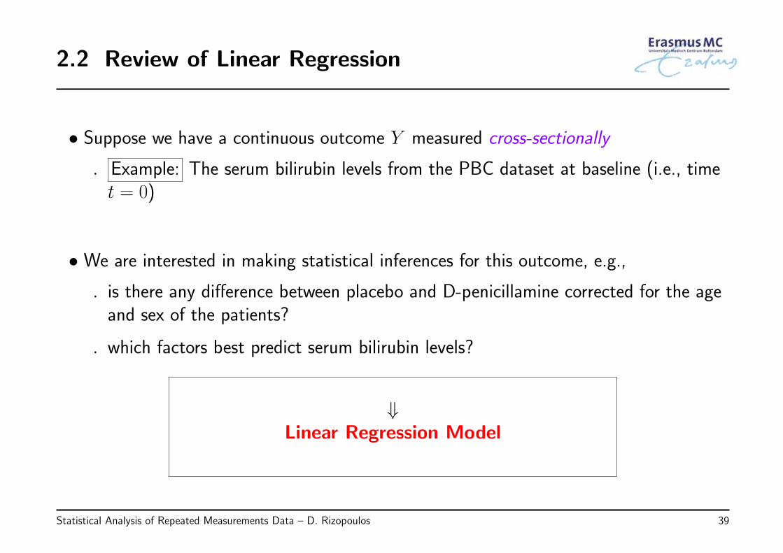
• Suppose we have a continuous outcome Y measured cross-sectionally
◃ Example: The serum bilirubin levels from the PBC dataset at baseline (i.e., timet = 0)
• We are interested in making statistical inferences for this outcome, e.g.,
◃ is there any difference between placebo and D-penicillamine corrected for the ageand sex of the patients?
◃ which factors best predict serum bilirubin levels?
⇓Linear Regression Model
Statistical Analysis of Repeated Measurements Data – D. Rizopoulos 39
2.2 Review of Linear Regression (cont’d)
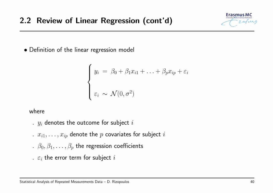
• Definition of the linear regression modelyi = β0 + β1xi1 + . . . + βpxip + εi
εi ∼ N (0, σ2)
where
◃ yi denotes the outcome for subject i
◃ xi1, . . . , xip denote the p covariates for subject i
◃ β0, β1, . . . , βp the regression coefficients
◃ εi the error term for subject i
Statistical Analysis of Repeated Measurements Data – D. Rizopoulos 40
2.2 Review of Linear Regression (cont’d)
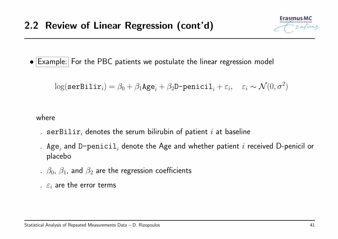
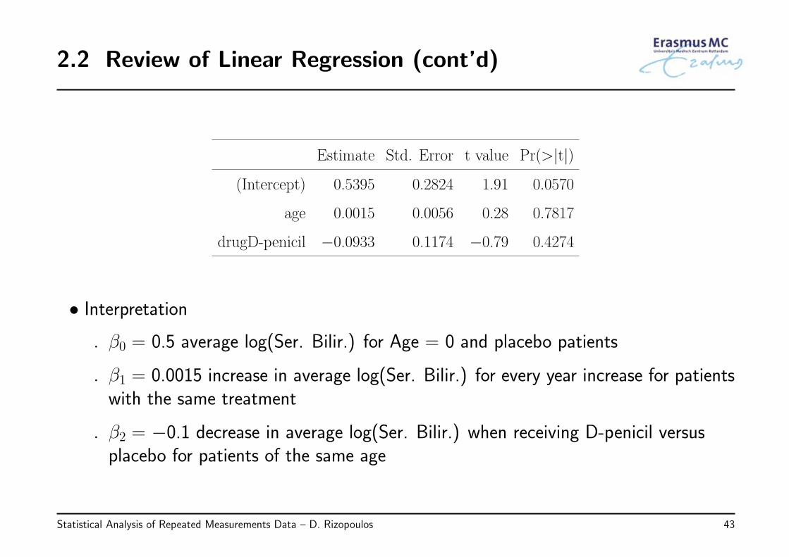
• Example: For the PBC patients we postulate the linear regression model
log(serBiliri) = β0 + β1Agei + β2D-penicili + εi, εi ∼ N (0, σ2)
where
◃ serBiliri denotes the serum bilirubin of patient i at baseline
◃ Agei and D-penicili denote the Age and whether patient i received D-penicil orplacebo
◃ β0, β1, and β2 are the regression coefficients
◃ εi are the error terms
Statistical Analysis of Repeated Measurements Data – D. Rizopoulos 41
2.2 Review of Linear Regression (cont’d)
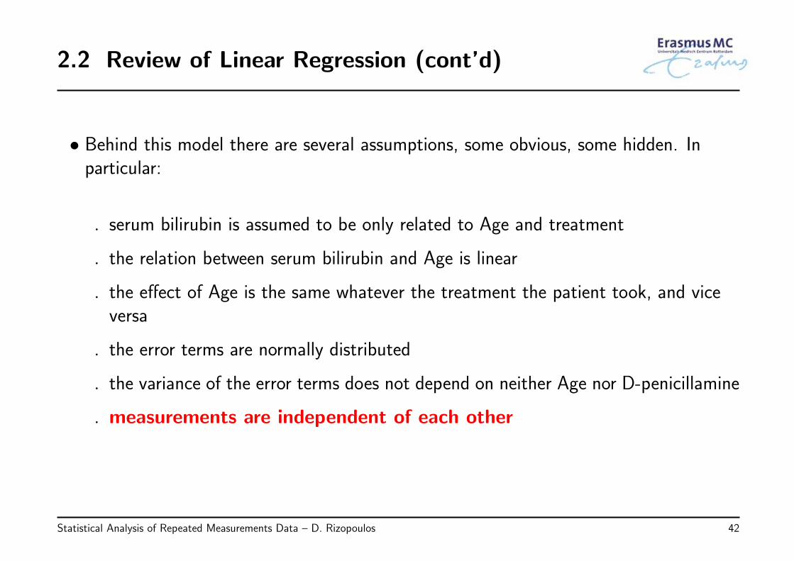
• Behind this model there are several assumptions, some obvious, some hidden. Inparticular:
◃ serum bilirubin is assumed to be only related to Age and treatment
◃ the relation between serum bilirubin and Age is linear
◃ the effect of Age is the same whatever the treatment the patient took, and viceversa
◃ the error terms are normally distributed
◃ the variance of the error terms does not depend on neither Age nor D-penicillamine
◃ measurements are independent of each other
Statistical Analysis of Repeated Measurements Data – D. Rizopoulos 42
2.2 Review of Linear Regression (cont’d)
Estimate Std. Error t value Pr(>|t|)
(Intercept) 0.5395 0.2824 1.91 0.0570
age 0.0015 0.0056 0.28 0.7817
drugD-penicil −0.0933 0.1174 −0.79 0.4274
• Interpretation
◃ β0 = 0.5 average log(Ser. Bilir.) for Age = 0 and placebo patients
◃ β1 = 0.0015 increase in average log(Ser. Bilir.) for every year increase for patientswith the same treatment
◃ β2 = −0.1 decrease in average log(Ser. Bilir.) when receiving D-penicil versusplacebo for patients of the same age
Statistical Analysis of Repeated Measurements Data – D. Rizopoulos 43
2.2 Review of Linear Regression (cont’d)
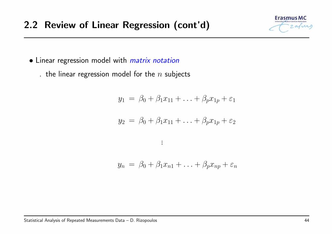
• Linear regression model with matrix notation
◃ the linear regression model for the n subjects
y1 = β0 + β1x11 + . . . + βpx1p + ε1
y2 = β0 + β1x11 + . . . + βpx1p + ε2
...
yn = β0 + β1xn1 + . . . + βpxnp + εn
Statistical Analysis of Repeated Measurements Data – D. Rizopoulos 44
2.2 Review of Linear Regression (cont’d)
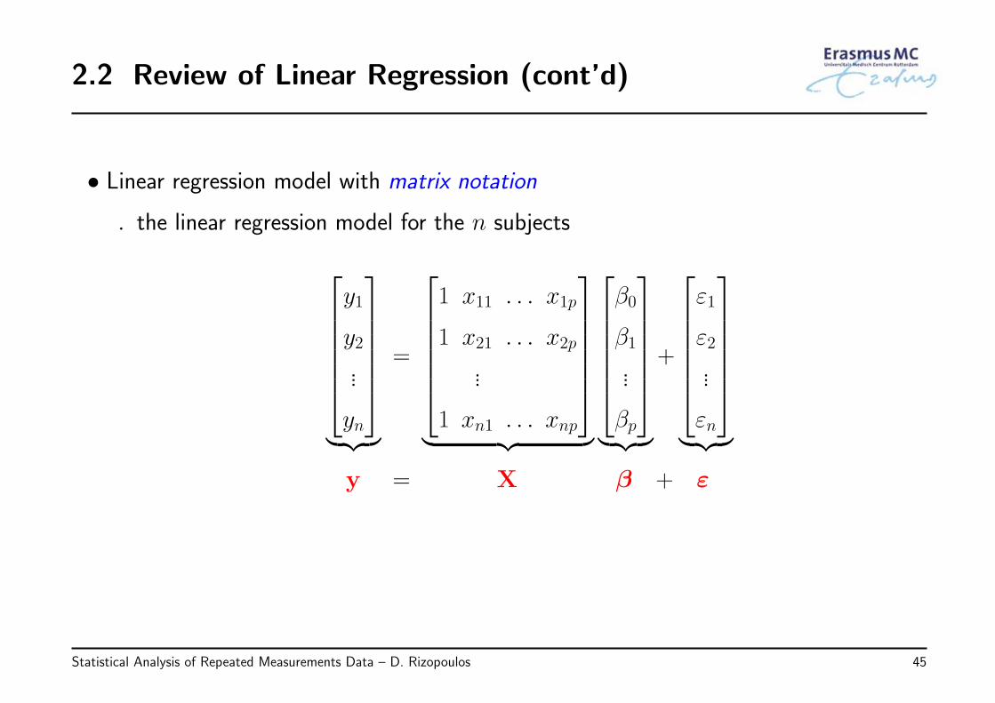
• Linear regression model with matrix notation
◃ the linear regression model for the n subjects
y1
y2...
yn
︸ ︷︷ ︸
=
1 x11 . . . x1p
1 x21 . . . x2p...
1 xn1 . . . xnp
︸ ︷︷ ︸
β0
β1...
βp
︸ ︷︷ ︸
+
ε1
ε2...
εn
︸ ︷︷ ︸
y = X β + ε
Statistical Analysis of Repeated Measurements Data – D. Rizopoulos 45
2.2 Review of Linear Regression (cont’d)
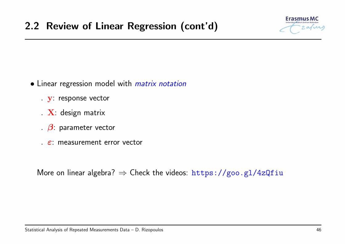
• Linear regression model with matrix notation
◃ y: response vector
◃ X: design matrix
◃ β: parameter vector
◃ ε: measurement error vector
More on linear algebra? ⇒ Check the videos: https://goo.gl/4zQfiu
Statistical Analysis of Repeated Measurements Data – D. Rizopoulos 46
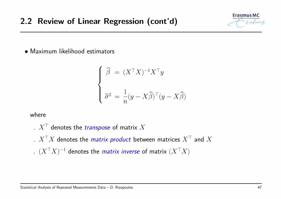
2.2 Review of Linear Regression (cont’d)
• Maximum likelihood estimatorsβ = (X⊤X)−1X⊤y
σ2 =1
n(y −Xβ)⊤(y −Xβ)
where
◃ X⊤ denotes the transpose of matrix X
◃ X⊤X denotes the matrix product between matrices X⊤ and X
◃ (X⊤X)−1 denotes the matrix inverse of matrix (X⊤X)
Statistical Analysis of Repeated Measurements Data – D. Rizopoulos 47
2.3 Marginal Models
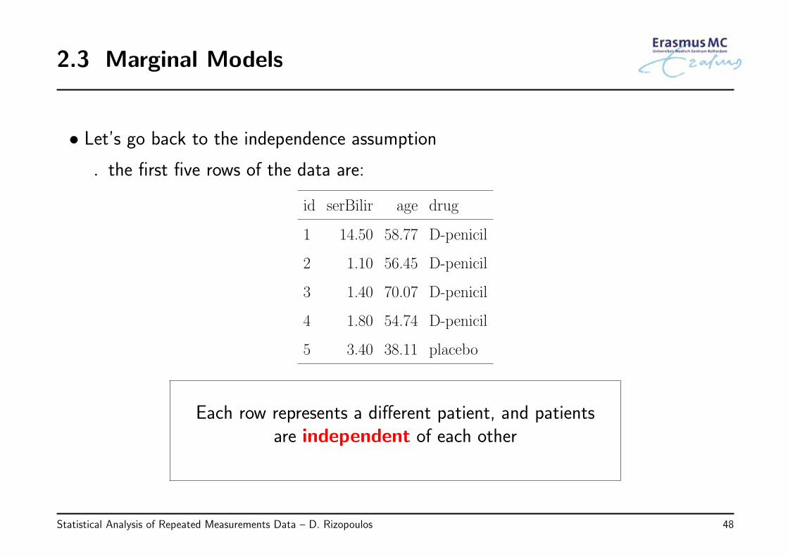
• Let’s go back to the independence assumption
◃ the first five rows of the data are:
id serBilir age drug
1 14.50 58.77 D-penicil
2 1.10 56.45 D-penicil
3 1.40 70.07 D-penicil
4 1.80 54.74 D-penicil
5 3.40 38.11 placebo
Each row represents a different patient, and patientsare independent of each other
Statistical Analysis of Repeated Measurements Data – D. Rizopoulos 48
2.3 Marginal Models (cont’d)
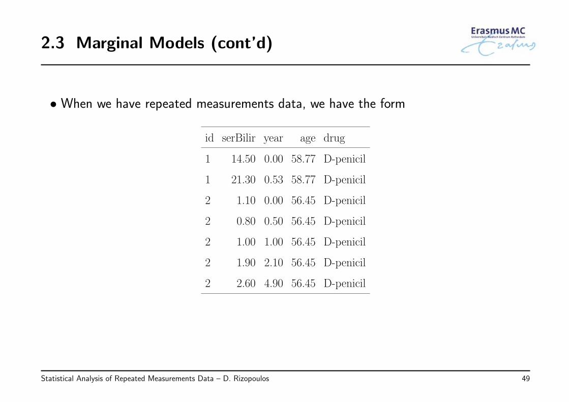
• When we have repeated measurements data, we have the form
id serBilir year age drug
1 14.50 0.00 58.77 D-penicil
1 21.30 0.53 58.77 D-penicil
2 1.10 0.00 56.45 D-penicil
2 0.80 0.50 56.45 D-penicil
2 1.00 1.00 56.45 D-penicil
2 1.90 2.10 56.45 D-penicil
2 2.60 4.90 56.45 D-penicil
Statistical Analysis of Repeated Measurements Data – D. Rizopoulos 49
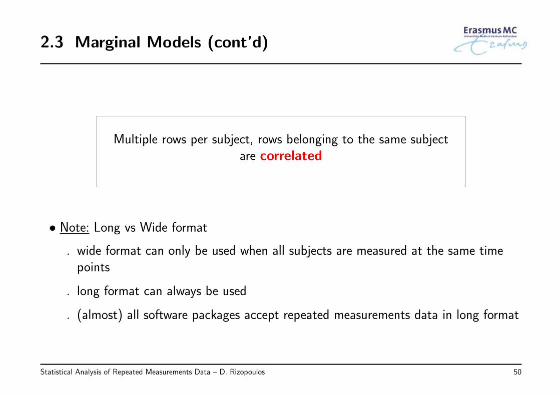
2.3 Marginal Models (cont’d)
Multiple rows per subject, rows belonging to the same subjectare correlated
• Note: Long vs Wide format
◃ wide format can only be used when all subjects are measured at the same timepoints
◃ long format can always be used
◃ (almost) all software packages accept repeated measurements data in long format
Statistical Analysis of Repeated Measurements Data – D. Rizopoulos 50
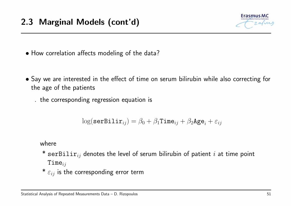
2.3 Marginal Models (cont’d)
• How correlation affects modeling of the data?
• Say we are interested in the effect of time on serum bilirubin while also correcting forthe age of the patients
◃ the corresponding regression equation is
log(serBilirij) = β0 + β1Timeij + β2Agei + εij
where
* serBilirij denotes the level of serum bilirubin of patient i at time pointTimeij
* εij is the corresponding error term
Statistical Analysis of Repeated Measurements Data – D. Rizopoulos 51
2.3 Marginal Models (cont’d)
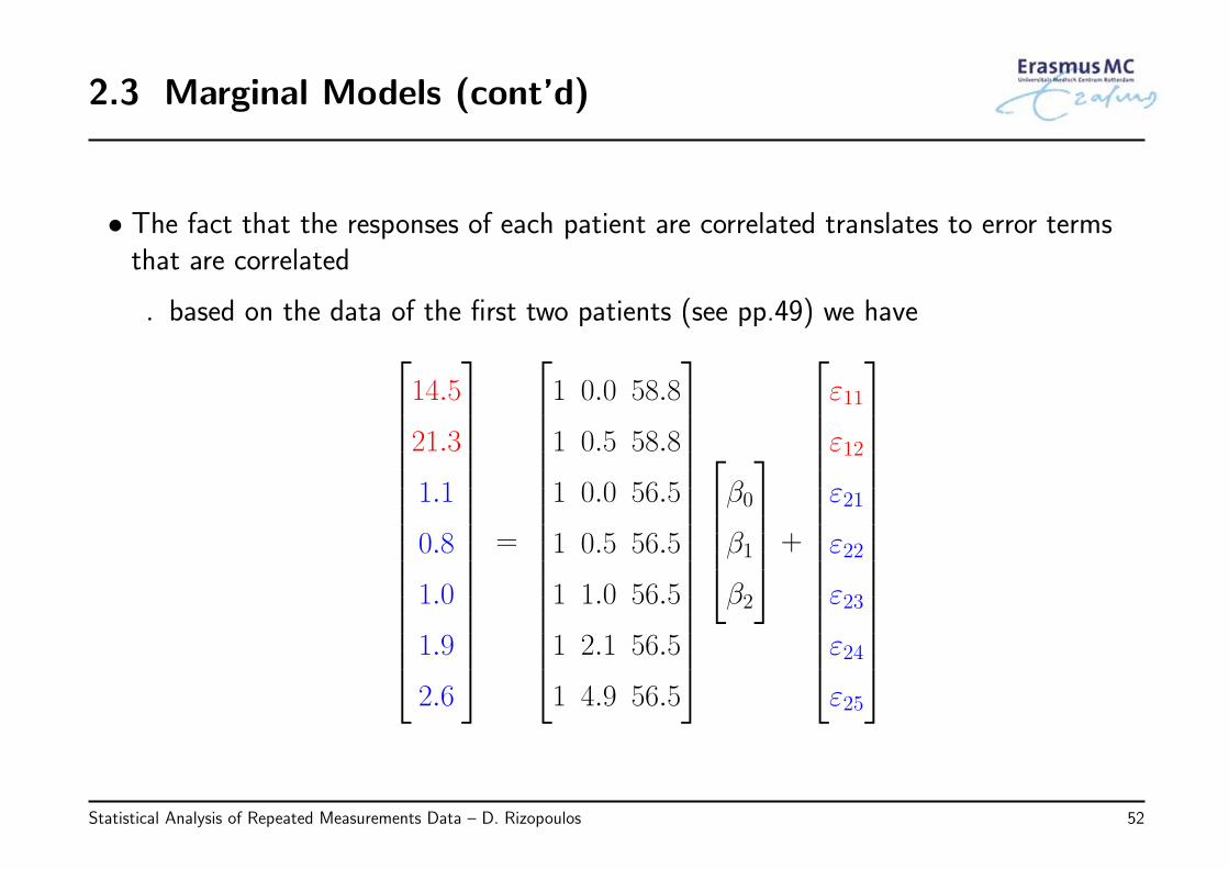
• The fact that the responses of each patient are correlated translates to error termsthat are correlated
◃ based on the data of the first two patients (see pp.49) we have
14.5
21.3
1.1
0.8
1.0
1.9
2.6
=
1 0.0 58.8
1 0.5 58.8
1 0.0 56.5
1 0.5 56.5
1 1.0 56.5
1 2.1 56.5
1 4.9 56.5
β0
β1
β2
+
ε11
ε12
ε21
ε22
ε23
ε24
ε25
Statistical Analysis of Repeated Measurements Data – D. Rizopoulos 52
2.3 Marginal Models (cont’d)
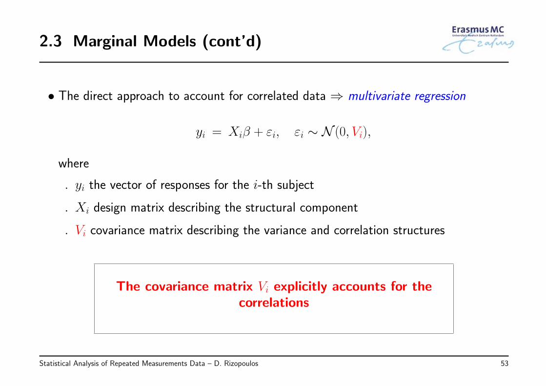
• The direct approach to account for correlated data ⇒ multivariate regression
yi = Xiβ + εi, εi ∼ N (0, Vi),
where
◃ yi the vector of responses for the i-th subject
◃ Xi design matrix describing the structural component
◃ Vi covariance matrix describing the variance and correlation structures
The covariance matrix Vi explicitly accounts for thecorrelations
Statistical Analysis of Repeated Measurements Data – D. Rizopoulos 53
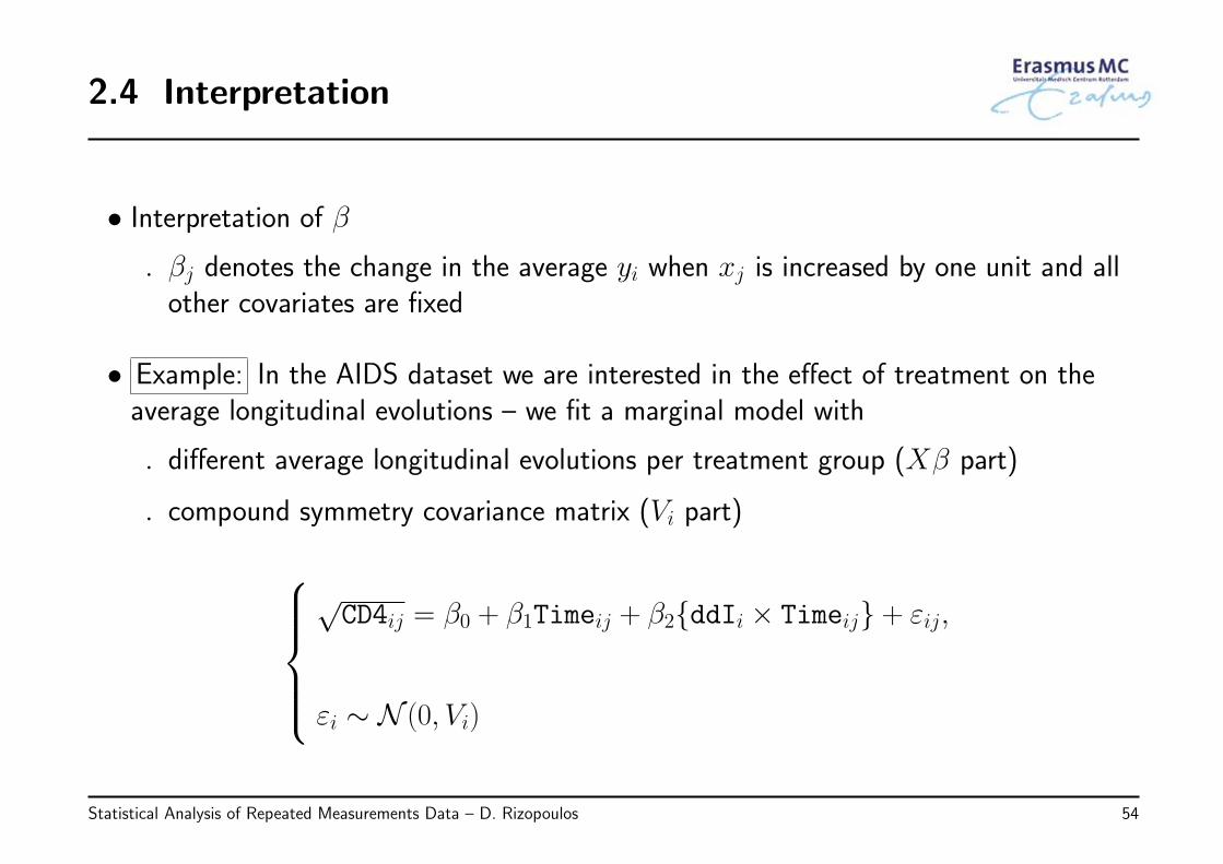
2.4 Interpretation
• Interpretation of β
◃ βj denotes the change in the average yi when xj is increased by one unit and allother covariates are fixed
• Example: In the AIDS dataset we are interested in the effect of treatment on theaverage longitudinal evolutions – we fit a marginal model with
◃ different average longitudinal evolutions per treatment group (Xβ part)
◃ compound symmetry covariance matrix (Vi part)
√CD4ij = β0 + β1Timeij + β2{ddIi × Timeij} + εij,
εi ∼ N (0, Vi)
Statistical Analysis of Repeated Measurements Data – D. Rizopoulos 54
2.4 Interpretation (cont’d)
Value Std.Err. t-value p-value
β0 7.189 0.221 32.593 < 0.001
β1 −0.156 0.017 −9.247 < 0.001
β2 0.016 0.024 0.662 0.508
◃ Coefficient β1: For patients in the ddC group, every month the average√CD4
changes by −0.156
◃ Coefficient β2:
* Is the difference of the time effect between ddI and ddC
* For patients in the ddI group, every month the average√CD4 changes by
(−0.156 + 0.016)
Statistical Analysis of Repeated Measurements Data – D. Rizopoulos 55
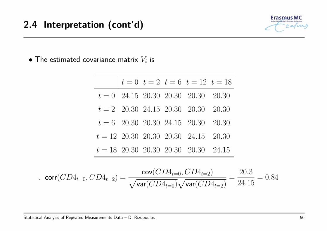
2.4 Interpretation (cont’d)
• The estimated covariance matrix Vi is
t = 0 t = 2 t = 6 t = 12 t = 18
t = 0 24.15 20.30 20.30 20.30 20.30
t = 2 20.30 24.15 20.30 20.30 20.30
t = 6 20.30 20.30 24.15 20.30 20.30
t = 12 20.30 20.30 20.30 24.15 20.30
t = 18 20.30 20.30 20.30 20.30 24.15
◃ corr(CD4t=0, CD4t=2) =cov(CD4t=0, CD4t=2)√
var(CD4t=0)√var(CD4t=2)
=20.3
24.15= 0.84
Statistical Analysis of Repeated Measurements Data – D. Rizopoulos 56
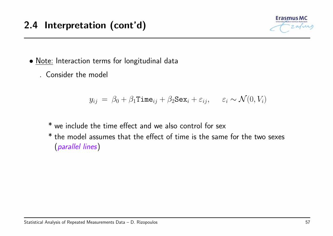
2.4 Interpretation (cont’d)
• Note: Interaction terms for longitudinal data
◃ Consider the model
yij = β0 + β1Timeij + β2Sexi + εij, εi ∼ N (0, Vi)
* we include the time effect and we also control for sex
* the model assumes that the effect of time is the same for the two sexes(parallel lines)
Statistical Analysis of Repeated Measurements Data – D. Rizopoulos 57
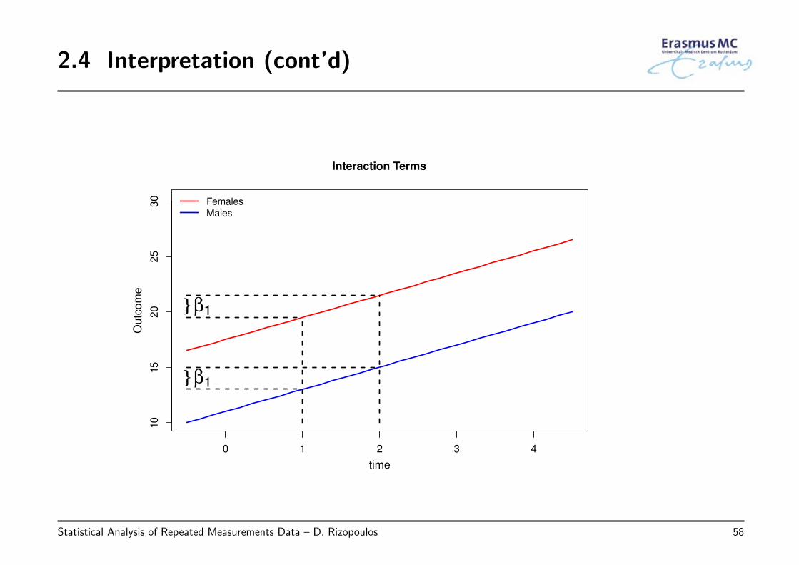
2.4 Interpretation (cont’d)
Interaction Terms
time
Ou
tco
me
0 1 2 3 4
10
15
20
25
30
}β1
}β1
Females
Males
Statistical Analysis of Repeated Measurements Data – D. Rizopoulos 58
2.4 Interpretation (cont’d)
• Note: Interaction terms for longitudinal data
◃ if we would like different longitudinal evolutions for the two sexes we need toinclude the interaction term
yij = β0 + β1Timeij + β2Sexi + β3{Sexi × Timeij} + εij, εi ∼ N (0, Vi)
Statistical Analysis of Repeated Measurements Data – D. Rizopoulos 59
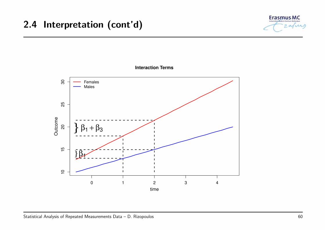
2.4 Interpretation (cont’d)
Interaction Terms
time
Ou
tco
me
0 1 2 3 4
10
15
20
25
30
}β1
} β1 + β3
Females
Males
Statistical Analysis of Repeated Measurements Data – D. Rizopoulos 60
2.4 Interpretation (cont’d)
• Note: Nonlinear terms for longitudinal data
◃ Consider the model
yij = β0 + β1Timeij + β2Sexi + εij, εi ∼ N (0, Vi)
* we include the time effect and we also control for sex
* the model assumes that the effect of time is linear
Statistical Analysis of Repeated Measurements Data – D. Rizopoulos 61
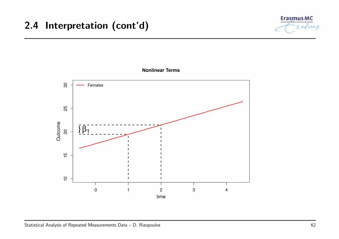
2.4 Interpretation (cont’d)
Nonlinear Terms
time
Ou
tco
me
0 1 2 3 4
10
15
20
25
30
}β1
Females
Statistical Analysis of Repeated Measurements Data – D. Rizopoulos 62
2.4 Interpretation (cont’d)
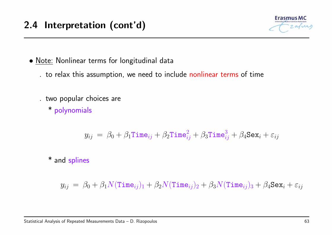
• Note: Nonlinear terms for longitudinal data
◃ to relax this assumption, we need to include nonlinear terms of time
◃ two popular choices are
* polynomials
yij = β0 + β1Timeij + β2Time2ij + β3Time
3ij + β4Sexi + εij
* and splines
yij = β0 + β1N(Timeij)1 + β2N(Timeij)2 + β3N(Timeij)3 + β4Sexi + εij
Statistical Analysis of Repeated Measurements Data – D. Rizopoulos 63
2.4 Interpretation (cont’d)
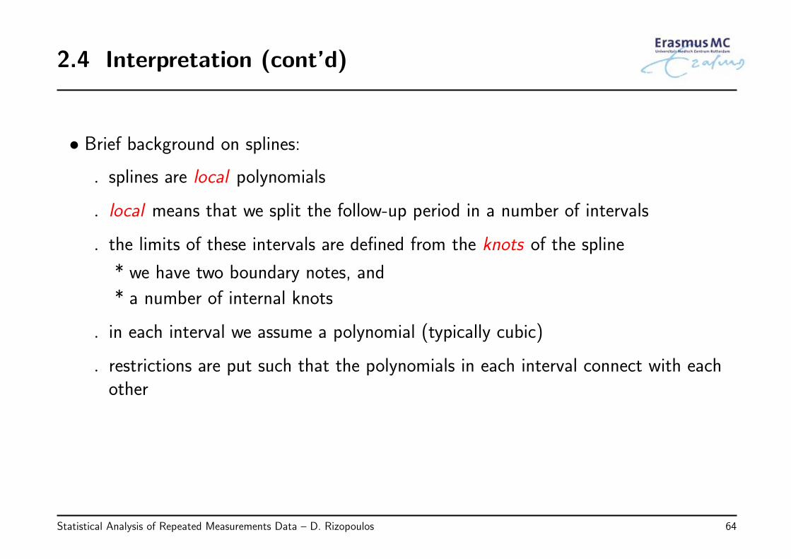
• Brief background on splines:
◃ splines are local polynomials
◃ local means that we split the follow-up period in a number of intervals
◃ the limits of these intervals are defined from the knots of the spline
* we have two boundary notes, and
* a number of internal knots
◃ in each interval we assume a polynomial (typically cubic)
◃ restrictions are put such that the polynomials in each interval connect with eachother
Statistical Analysis of Repeated Measurements Data – D. Rizopoulos 64
2.4 Interpretation (cont’d)
• In both polynomials and splines, increasing
◃ the degree in the former, and
◃ the number of internal knots in the latter
allows the time effect to be modeled more flexibly
• However, we should not overdo it because of the risk of over-fitting
◃ in the majority of the cases, a 2nd or 3rd degree polynomial or 2 or 3 internalknots are sufficient to capture nonlinearities
From the two approaches, splines arepreferable
Statistical Analysis of Repeated Measurements Data – D. Rizopoulos 65
2.4 Interpretation (cont’d)
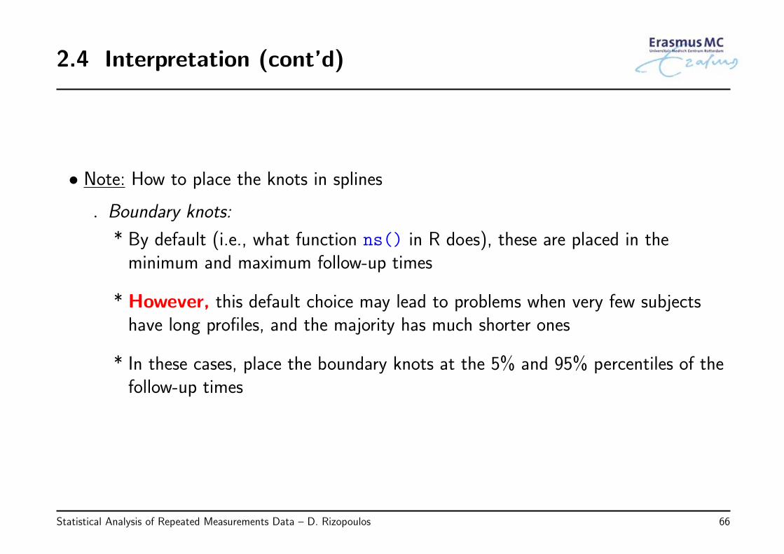
• Note: How to place the knots in splines
◃ Boundary knots:
* By default (i.e., what function ns() in R does), these are placed in theminimum and maximum follow-up times
* However, this default choice may lead to problems when very few subjectshave long profiles, and the majority has much shorter ones
* In these cases, place the boundary knots at the 5% and 95% percentiles of thefollow-up times
Statistical Analysis of Repeated Measurements Data – D. Rizopoulos 66
2.4 Interpretation (cont’d)
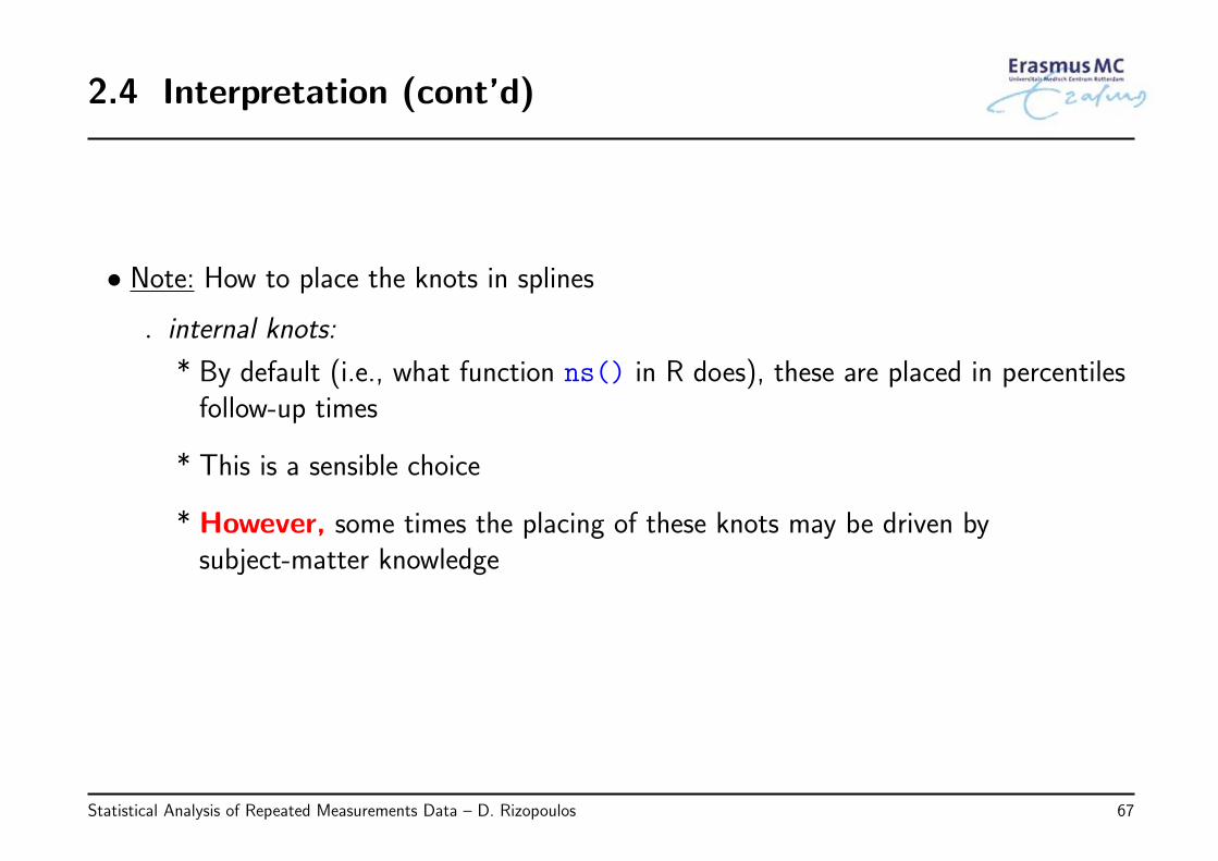
• Note: How to place the knots in splines
◃ internal knots:
* By default (i.e., what function ns() in R does), these are placed in percentilesfollow-up times
* This is a sensible choice
* However, some times the placing of these knots may be driven bysubject-matter knowledge
Statistical Analysis of Repeated Measurements Data – D. Rizopoulos 67
2.4 Interpretation (cont’d)
• Communicating a model with complex terms: Due to the elaborate structureof repeated measurements data it is often required to include complex terms in amodel
◃ interaction terms (e.g., between baseline and time-varying predictors)
◃ nonlinear terms (e.g., nonlinear evolutions over time modeled with polynomials orsplines)
• In such cases the regression coefficients β we obtain in the output do not often havea straightforward interpretation
Statistical Analysis of Repeated Measurements Data – D. Rizopoulos 68
2.4 Interpretation (cont’d)
• To overcome this issue we can use effect plots
◃ this is a figure that depicts the average outcome along with 95% confidenceintervals for specific combinations of the predictors’ levels
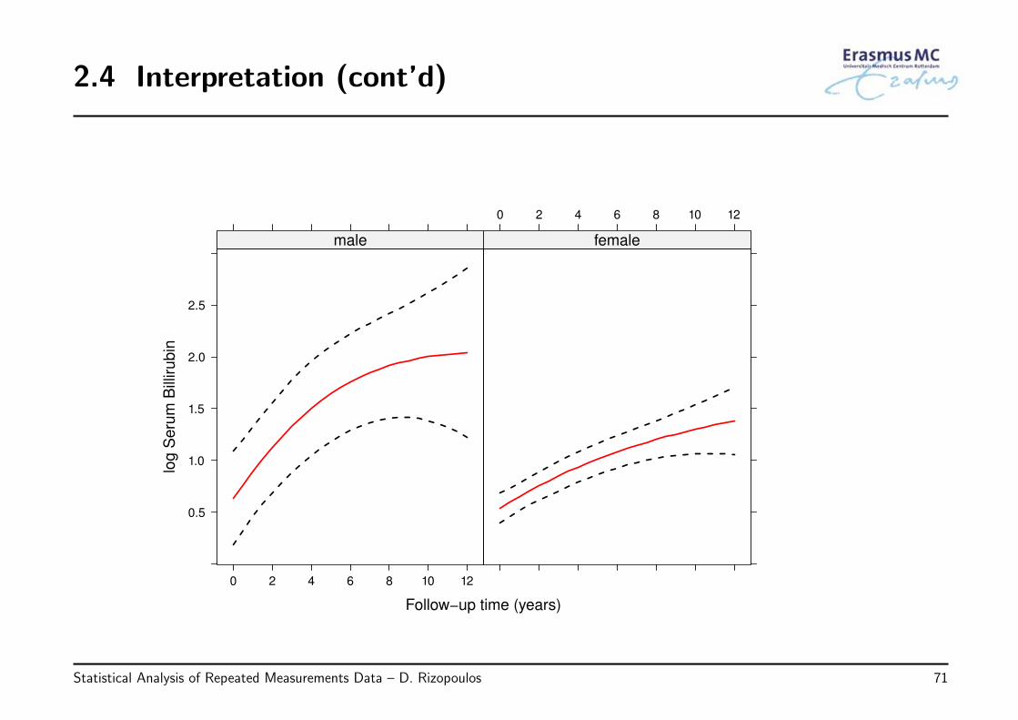
• Example: We have fitted the following model to the PBC dataset:
log(serBilirij) = β0 + β1N(Timeij)1 + β2N(Timeij)2 + β3Femalei + β4Agei+
β5{Femalei ×N(Timeij)1} + β6{Femalei ×N(Timeij)2}+β7{Femalei × Agei} + εij
εi ∼ N (0, Vi) Vi has a continuous AR1 structure
Statistical Analysis of Repeated Measurements Data – D. Rizopoulos 69
2.4 Interpretation (cont’d)
• The terms N(Timeij)1 and N(Timeij)2 denote the basis for a natural cubic splinewith two degrees of freedom to model possible nonlinearities in the time effect
• In this model not all coefficients have a direct interpretation in isolation
• Hence to understand the model we depict
◃ how the average longitudinal profiles evolve over time,
◃ separately for males and females, and
◃ for the average age of 49 years old (in the app different ages can be selected)
◃ including also the corresponding 95% pointwise confidence intervals
Statistical Analysis of Repeated Measurements Data – D. Rizopoulos 70
2.4 Interpretation (cont’d)
Follow−up time (years)
log
Se
rum
Bill
iru
bin
0.5
1.0
1.5
2.0
2.5
0 2 4 6 8 10 12
male
0 2 4 6 8 10 12
female
Statistical Analysis of Repeated Measurements Data – D. Rizopoulos 71
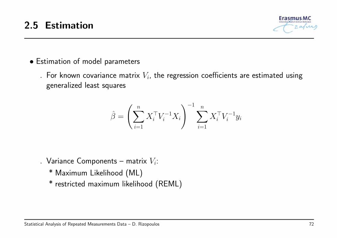
2.5 Estimation
• Estimation of model parameters
◃ For known covariance matrix Vi, the regression coefficients are estimated usinggeneralized least squares
β =
(n∑i=1
X⊤i V
−1i Xi
)−1 n∑i=1
X⊤i V
−1i yi
◃ Variance Components – matrix Vi:
* Maximum Likelihood (ML)
* restricted maximum likelihood (REML)
Statistical Analysis of Repeated Measurements Data – D. Rizopoulos 72
2.5 Estimation (cont’d)
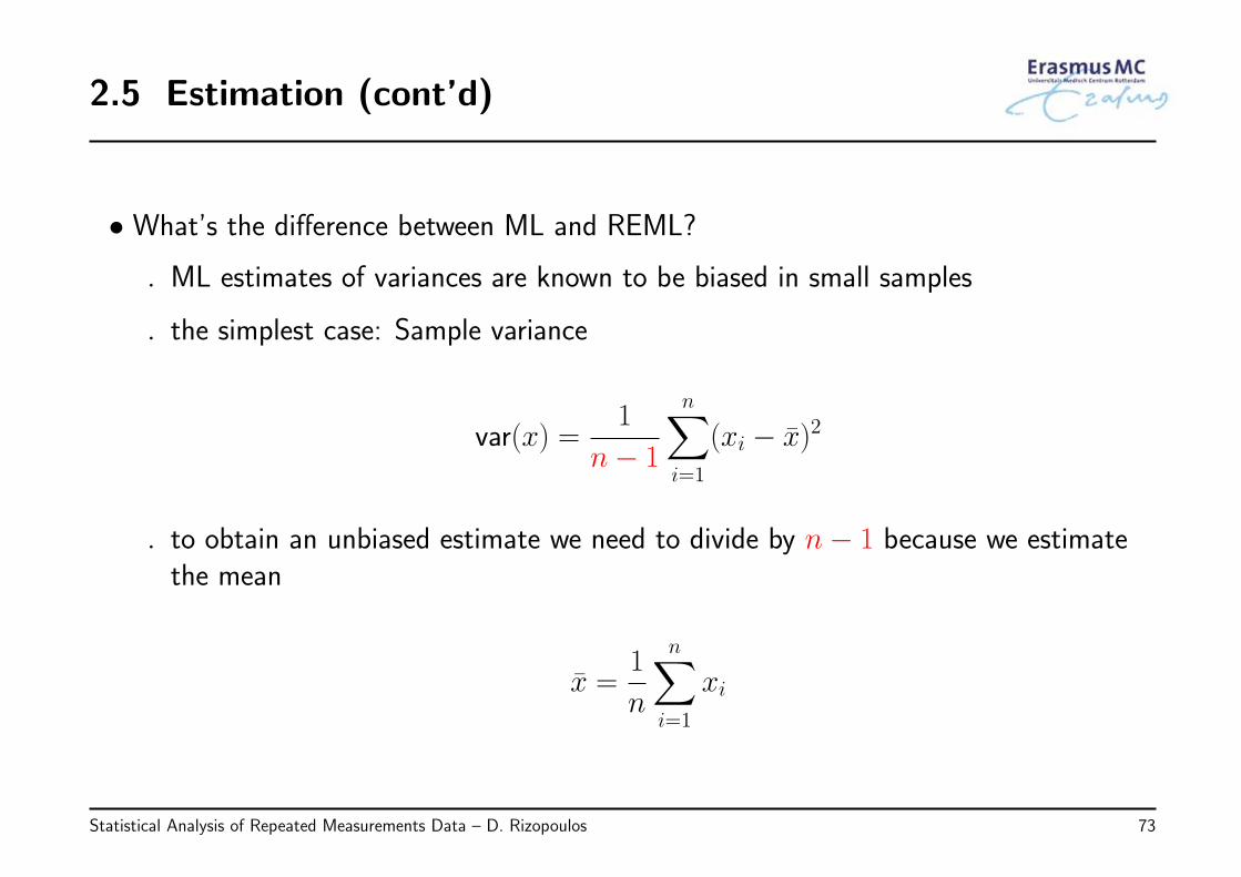
• What’s the difference between ML and REML?
◃ ML estimates of variances are known to be biased in small samples
◃ the simplest case: Sample variance
var(x) =1
n− 1
n∑i=1
(xi − x)2
◃ to obtain an unbiased estimate we need to divide by n− 1 because we estimatethe mean
x =1
n
n∑i=1
xi
Statistical Analysis of Repeated Measurements Data – D. Rizopoulos 73
2.5 Estimation (cont’d)
The REML estimation is a generalization of this idea
• It provides unbiased estimates of the parameters in the covariance matrix Vi in smallsamples
• Example: To illustrate the difference between REML and ML we consider fitting thesame model for the AIDS dataset we have seen before but using only the first 50 rows
Statistical Analysis of Repeated Measurements Data – D. Rizopoulos 74
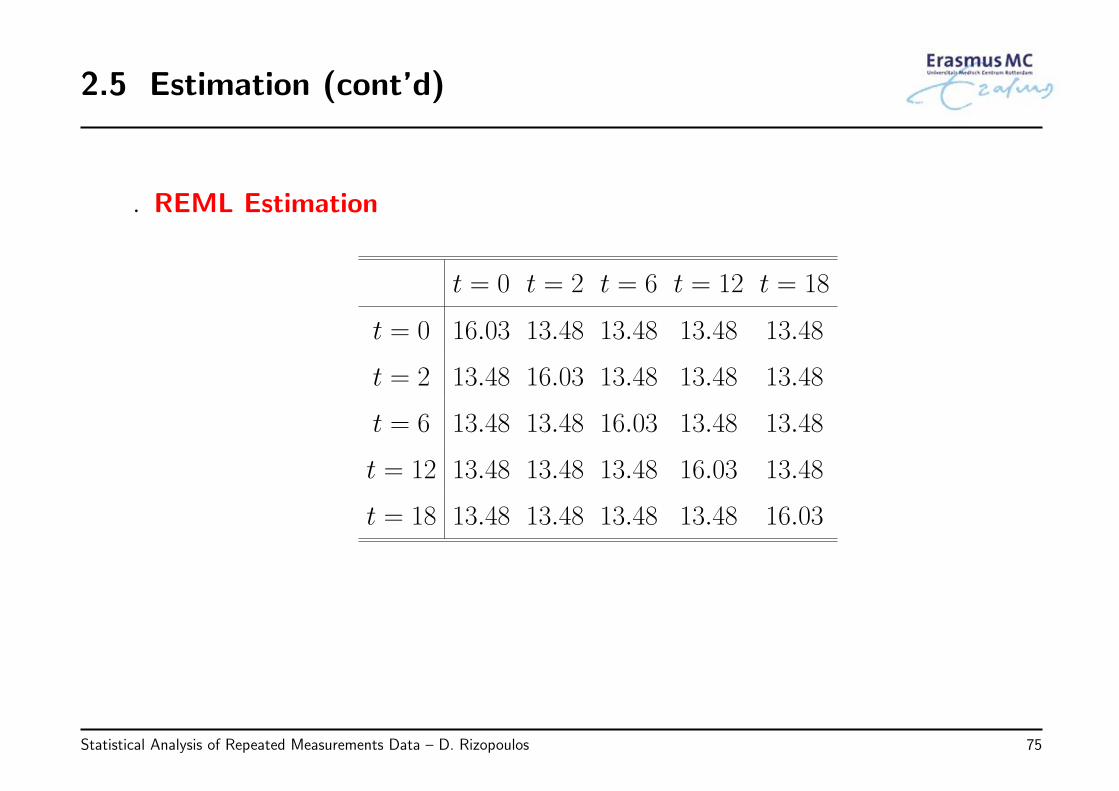
2.5 Estimation (cont’d)
◃ REML Estimation
t = 0 t = 2 t = 6 t = 12 t = 18
t = 0 16.03 13.48 13.48 13.48 13.48
t = 2 13.48 16.03 13.48 13.48 13.48
t = 6 13.48 13.48 16.03 13.48 13.48
t = 12 13.48 13.48 13.48 16.03 13.48
t = 18 13.48 13.48 13.48 13.48 16.03
Statistical Analysis of Repeated Measurements Data – D. Rizopoulos 75
2.5 Estimation (cont’d)
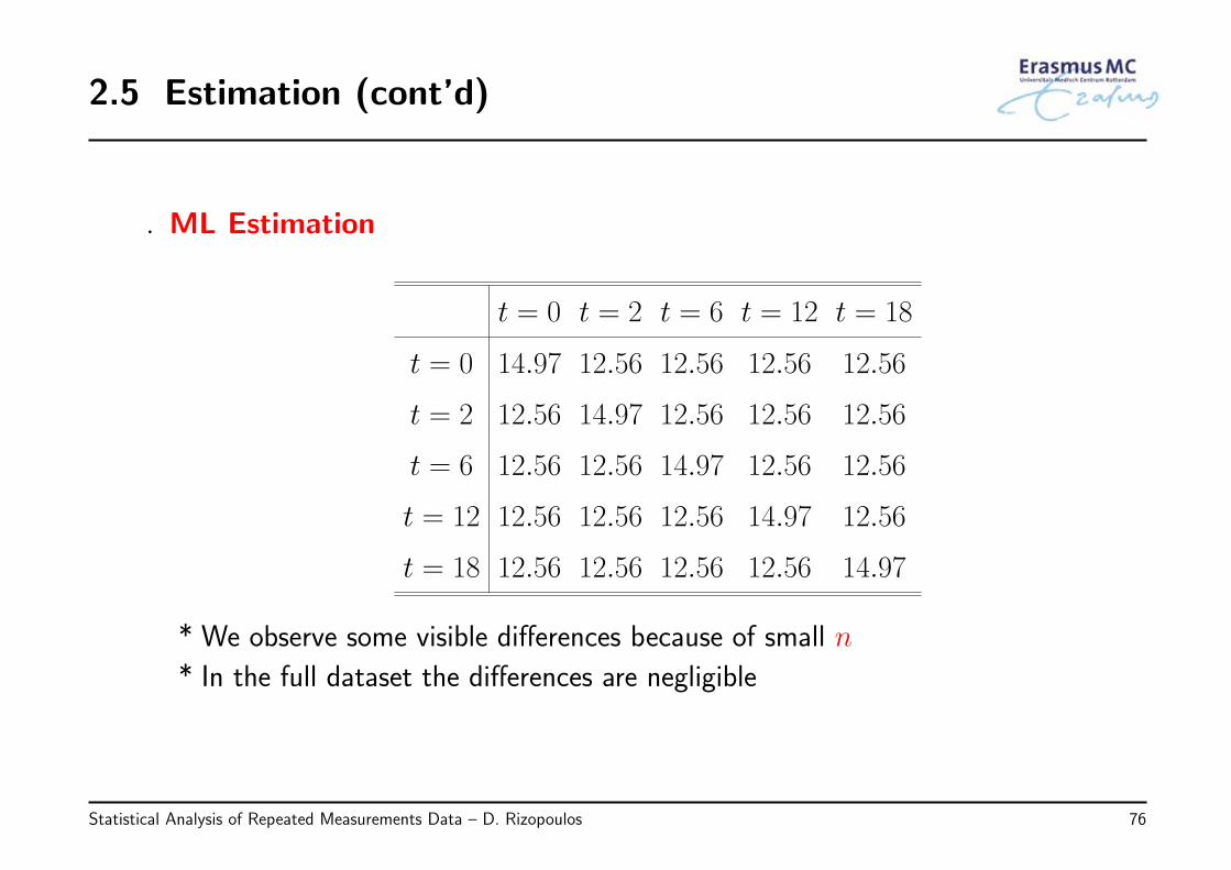
◃ ML Estimation
t = 0 t = 2 t = 6 t = 12 t = 18
t = 0 14.97 12.56 12.56 12.56 12.56
t = 2 12.56 14.97 12.56 12.56 12.56
t = 6 12.56 12.56 14.97 12.56 12.56
t = 12 12.56 12.56 12.56 14.97 12.56
t = 18 12.56 12.56 12.56 12.56 14.97
* We observe some visible differences because of small n
* In the full dataset the differences are negligible
Statistical Analysis of Repeated Measurements Data – D. Rizopoulos 76
2.5 Estimation (cont’d)
• Features of REML estimation:
◃ Available in all software that fit marginal and mixed effects models
◃ The way it works is by applying a transformation in the longitudinal outcome ybased on the chosen structure of the design matrix X(i.e., which predictors you have included in the model)
◃ Hence, we cannot compare the likelihoods of models fitted withREML and have different Xβ part
Statistical Analysis of Repeated Measurements Data – D. Rizopoulos 77
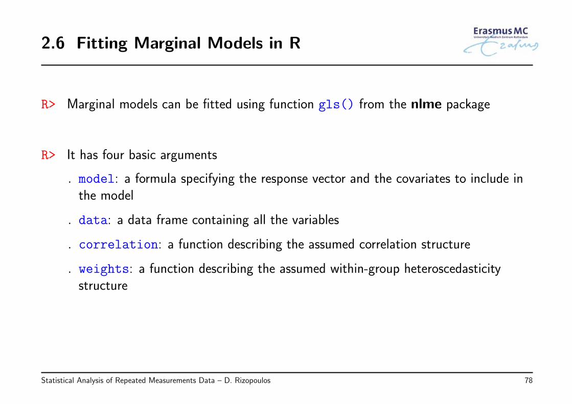
2.6 Fitting Marginal Models in R
R> Marginal models can be fitted using function gls() from the nlme package
R> It has four basic arguments
◃ model: a formula specifying the response vector and the covariates to include inthe model
◃ data: a data frame containing all the variables
◃ correlation: a function describing the assumed correlation structure
◃ weights: a function describing the assumed within-group heteroscedasticitystructure
Statistical Analysis of Repeated Measurements Data – D. Rizopoulos 78
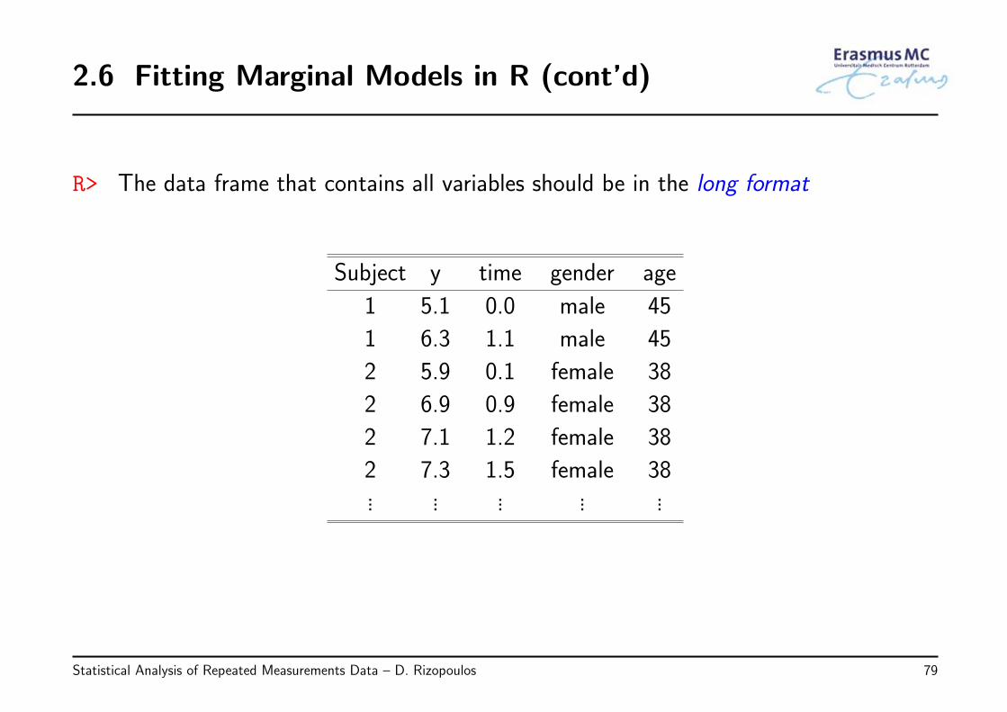
2.6 Fitting Marginal Models in R (cont’d)
R> The data frame that contains all variables should be in the long format
Subject y time gender age
1 5.1 0.0 male 45
1 6.3 1.1 male 45
2 5.9 0.1 female 38
2 6.9 0.9 female 38
2 7.1 1.2 female 38
2 7.3 1.5 female 38... ... ... ... ...
Statistical Analysis of Repeated Measurements Data – D. Rizopoulos 79
2.6 Fitting Marginal Models in R (cont’d)
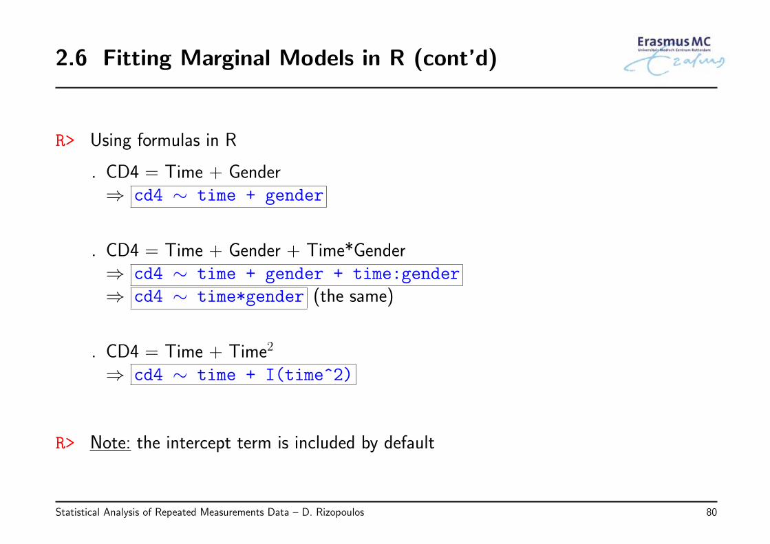
R> Using formulas in R
◃ CD4 = Time + Gender⇒ cd4 ∼ time + gender
◃ CD4 = Time + Gender + Time*Gender⇒ cd4 ∼ time + gender + time:gender
⇒ cd4 ∼ time*gender (the same)
◃ CD4 = Time + Time2
⇒ cd4 ∼ time + I(time^2)
R> Note: the intercept term is included by default
Statistical Analysis of Repeated Measurements Data – D. Rizopoulos 80
2.6 Fitting Marginal Models in R (cont’d)
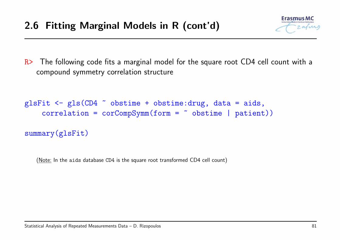
R> The following code fits a marginal model for the square root CD4 cell count with acompound symmetry correlation structure
glsFit <- gls(CD4 ~ obstime + obstime:drug, data = aids,
correlation = corCompSymm(form = ~ obstime | patient))
summary(glsFit)
(Note: In the aids database CD4 is the square root transformed CD4 cell count)
Statistical Analysis of Repeated Measurements Data – D. Rizopoulos 81
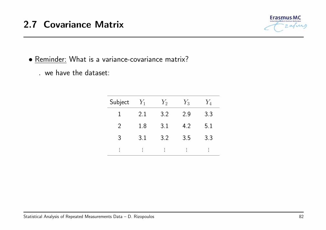
2.7 Covariance Matrix
• Reminder: What is a variance-covariance matrix?
◃ we have the dataset:
Subject Y1 Y2 Y3 Y4
1 2.1 3.2 2.9 3.3
2 1.8 3.1 4.2 5.1
3 3.1 3.2 3.5 3.3
... ... ... ... ...
Statistical Analysis of Repeated Measurements Data – D. Rizopoulos 82
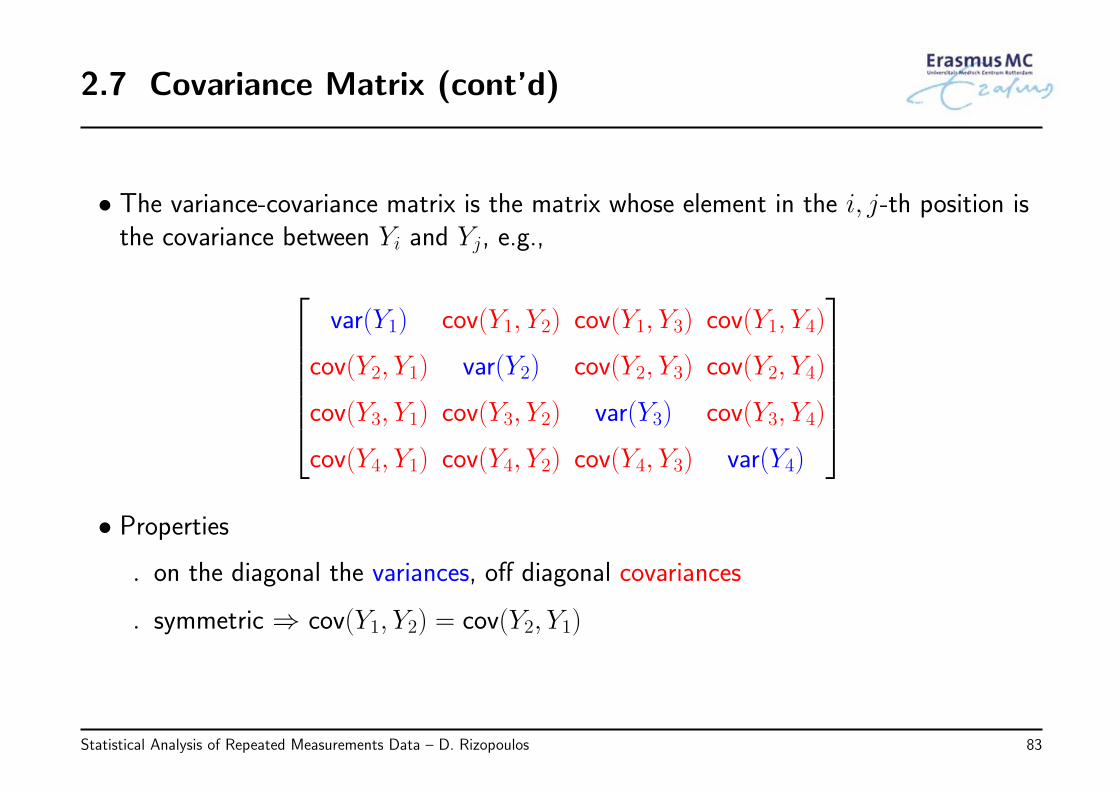
2.7 Covariance Matrix (cont’d)
• The variance-covariance matrix is the matrix whose element in the i, j-th position isthe covariance between Yi and Yj, e.g.,
var(Y1) cov(Y1, Y2) cov(Y1, Y3) cov(Y1, Y4)
cov(Y2, Y1) var(Y2) cov(Y2, Y3) cov(Y2, Y4)
cov(Y3, Y1) cov(Y3, Y2) var(Y3) cov(Y3, Y4)
cov(Y4, Y1) cov(Y4, Y2) cov(Y4, Y3) var(Y4)
• Properties
◃ on the diagonal the variances, off diagonal covariances
◃ symmetric ⇒ cov(Y1, Y2) = cov(Y2, Y1)
Statistical Analysis of Repeated Measurements Data – D. Rizopoulos 83
2.7 Covariance Matrix (cont’d)
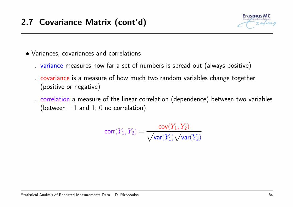
• Variances, covariances and correlations
◃ variance measures how far a set of numbers is spread out (always positive)
◃ covariance is a measure of how much two random variables change together(positive or negative)
◃ correlation a measure of the linear correlation (dependence) between two variables(between −1 and 1; 0 no correlation)
corr(Y1, Y2) =cov(Y1, Y2)√
var(Y1)√
var(Y2)
Statistical Analysis of Repeated Measurements Data – D. Rizopoulos 84
2.7 Covariance Matrix (cont’d)
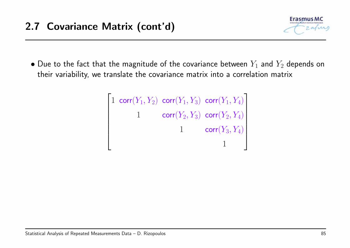
• Due to the fact that the magnitude of the covariance between Y1 and Y2 depends ontheir variability, we translate the covariance matrix into a correlation matrix
1 corr(Y1, Y2) corr(Y1, Y3) corr(Y1, Y4)
1 corr(Y2, Y3) corr(Y2, Y4)
1 corr(Y3, Y4)
1
Statistical Analysis of Repeated Measurements Data – D. Rizopoulos 85
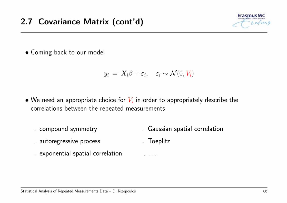
2.7 Covariance Matrix (cont’d)
• Coming back to our model
yi = Xiβ + εi, εi ∼ N (0, Vi)
• We need an appropriate choice for Vi in order to appropriately describe thecorrelations between the repeated measurements
◃ compound symmetry ◃ Gaussian spatial correlation
◃ autoregressive process ◃ Toeplitz
◃ exponential spatial correlation ◃ . . .
Statistical Analysis of Repeated Measurements Data – D. Rizopoulos 86
2.7 Covariance Matrix (cont’d)
• Let’s see some of those
◃ General/Unstructured σ21 σ12 σ13
σ12 σ22 σ23
σ13 σ23 σ23
◃ Diagonal
σ21 0 0
0 σ22 0
0 0 σ23
or
σ2 0 0
0 σ2 0
0 0 σ2
Statistical Analysis of Repeated Measurements Data – D. Rizopoulos 87
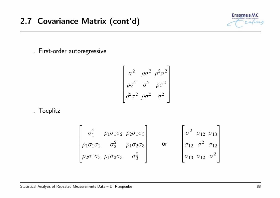
2.7 Covariance Matrix (cont’d)
◃ First-order autoregressive
σ2 ρσ2 ρ2σ2
ρσ2 σ2 ρσ2
ρ2σ2 ρσ2 σ2
◃ Toeplitz
σ21 ρ1σ1σ2 ρ2σ1σ3
ρ1σ1σ2 σ22 ρ1σ2σ3
ρ2σ1σ3 ρ1σ2σ3 σ23
or
σ2 σ12 σ13
σ12 σ2 σ12
σ13 σ12 σ2
Statistical Analysis of Repeated Measurements Data – D. Rizopoulos 88
2.7 Covariance Matrix (cont’d)
• The aforementioned structures for the covariance matrix are applicable in cases wehave discrete and equally spaced time points
• For continuous time and unbalanced data, alternative options are:
◃ continuous AR1
◃ exponential serial correlation
◃ linear correlation
◃ Gaussian serial correlation
Statistical Analysis of Repeated Measurements Data – D. Rizopoulos 89
2.7 Covariance Matrix (cont’d)
• These serial correlation structures are defined using the semi-variogram
◃ which we are not going to cover here because it is a bit technical (more info inany standard text for mixed models / longitudinal data analysis)
• The basic assumption is that correlations decay with the time lag |ti − tj| ⇒measurements at closer time points are more strongly correlated than measurementsat more distant time points
◃ the aforementioned structures for unbalanced data have one parameter thatcontrols how the correlations decay over time
Statistical Analysis of Repeated Measurements Data – D. Rizopoulos 90
2.7 Covariance Matrix (cont’d)
• Notes: On building covariance matrices
◃ variance function: in some cases, and especially for longitudinal data, it may notbe reasonable to assume that the variance of the outcome remains constant overtime
* we have seen versions of heteroscedastic covariance matrices, but these are onlyapplicable when we have balanced data and few time points
* for unbalanced designs we can specify other variance functions, e.g., thatvariances increase linearly or exponentially over time
◃ correlation at the same point: is it always reasonable that the correlation of theoutcome at the same point is set to 1?
Statistical Analysis of Repeated Measurements Data – D. Rizopoulos 91
2.7 Covariance Matrix (cont’d)
• Let’s try the app. . .
Statistical Analysis of Repeated Measurements Data – D. Rizopoulos 92
2.8 Model Building
• We have seen that marginal models consist of two parts:
◃ Mean part – Xβ: that describes how covariates we have put in the model explainthe average of the repeated measurements
◃ Covariance part – Vi: assumed covariance structure between the repeatedmeasurements
• In the majority of the cases scientific interest focuses on the mean part
However, to obtain valid and efficient inferences for themean part, the covariance part needs to be adequately
specified
Statistical Analysis of Repeated Measurements Data – D. Rizopoulos 93
2.8 Model Building (cont’d)
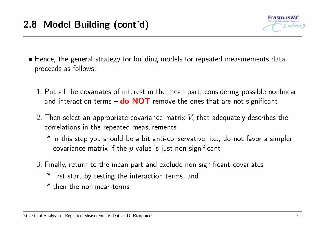
• Hence, the general strategy for building models for repeated measurements dataproceeds as follows:
1. Put all the covariates of interest in the mean part, considering possible nonlinearand interaction terms – do NOT remove the ones that are not significant
2. Then select an appropriate covariance matrix Vi that adequately describes thecorrelations in the repeated measurements
* in this step you should be a bit anti-conservative, i.e., do not favor a simplercovariance matrix if the p-value is just non-significant
3. Finally, return to the mean part and exclude non significant covariates
* first start by testing the interaction terms, and
* then the nonlinear terms
Statistical Analysis of Repeated Measurements Data – D. Rizopoulos 94
2.8 Model Building (cont’d)
• How many coefficients can we reliably estimate in the mean part?
• It depends on how strong the correlations between the repeated measurements are
◃ weak correlations ⇒ N/10 (N total number of measurements)
◃ strong correlations ⇒ n/10 (n number of subjects)
Statistical Analysis of Repeated Measurements Data – D. Rizopoulos 95
2.9 Hypothesis Testing
• Having fitted a marginal model using maximum likelihood we can use standardinferential tools for performing hypothesis testing
◃ Wald tests / t-tests / F-tests
◃ Score tests
◃ Likelihood ratio tests
• Following the model building strategy described above, we will
◃ first, describe how we can choose the appropriate covariance matrix, and
◃ then focus on hypothesis testing for the mean part of the model
Statistical Analysis of Repeated Measurements Data – D. Rizopoulos 96
2.9 Hypothesis Testing (cont’d)
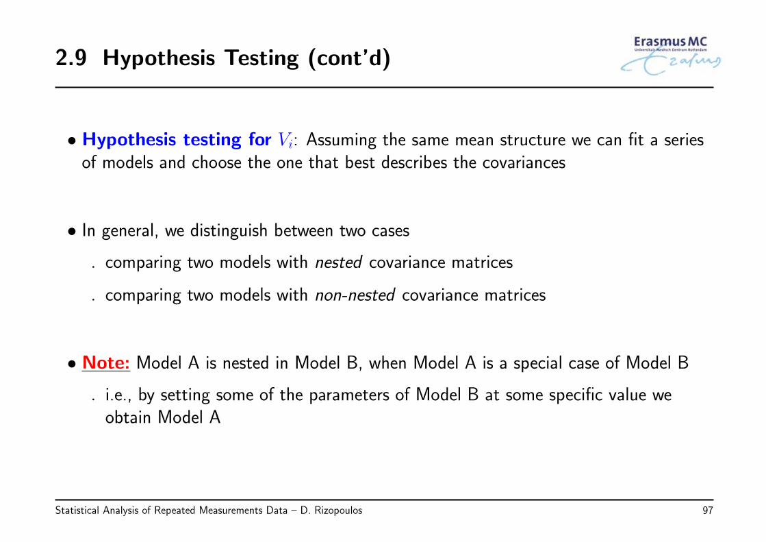
• Hypothesis testing for Vi: Assuming the same mean structure we can fit a seriesof models and choose the one that best describes the covariances
• In general, we distinguish between two cases
◃ comparing two models with nested covariance matrices
◃ comparing two models with non-nested covariance matrices
• Note: Model A is nested in Model B, when Model A is a special case of Model B
◃ i.e., by setting some of the parameters of Model B at some specific value weobtain Model A
Statistical Analysis of Repeated Measurements Data – D. Rizopoulos 97
2.9 Hypothesis Testing (cont’d)
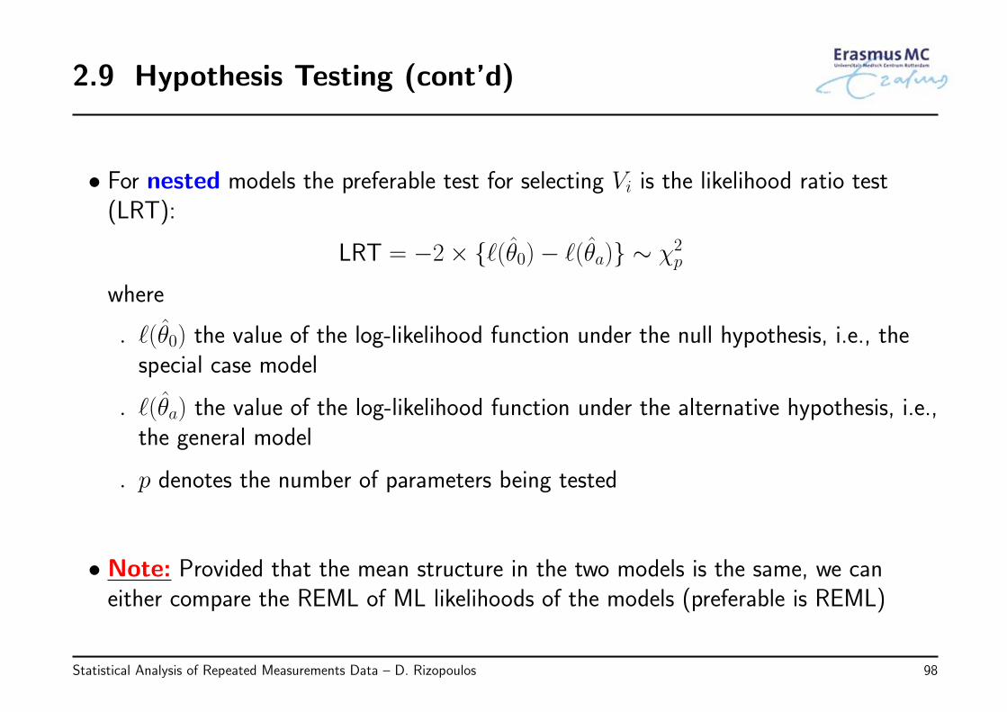
• For nested models the preferable test for selecting Vi is the likelihood ratio test(LRT):
LRT = −2× {ℓ(θ0)− ℓ(θa)} ∼ χ2p
where
◃ ℓ(θ0) the value of the log-likelihood function under the null hypothesis, i.e., thespecial case model
◃ ℓ(θa) the value of the log-likelihood function under the alternative hypothesis, i.e.,the general model
◃ p denotes the number of parameters being tested
• Note: Provided that the mean structure in the two models is the same, we caneither compare the REML of ML likelihoods of the models (preferable is REML)
Statistical Analysis of Repeated Measurements Data – D. Rizopoulos 98
2.9 Hypothesis Testing (cont’d)
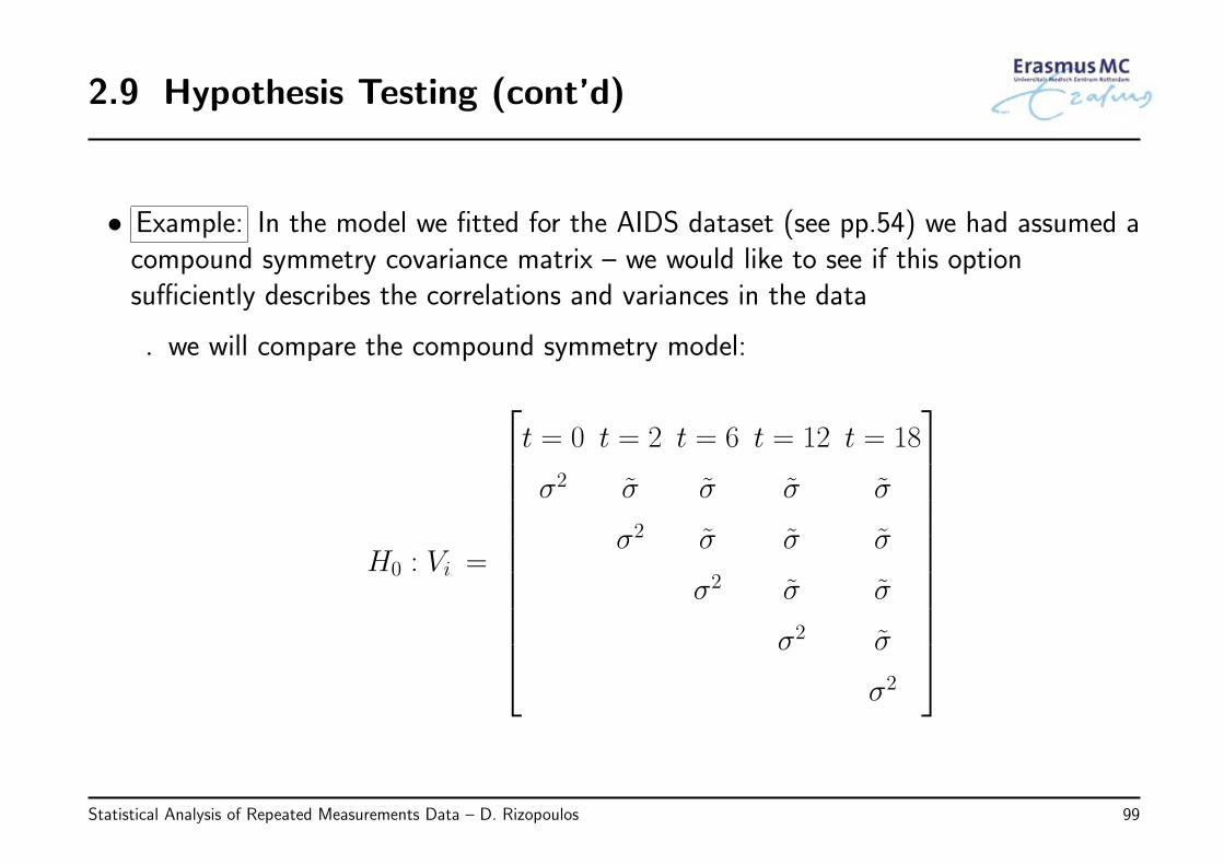
• Example: In the model we fitted for the AIDS dataset (see pp.54) we had assumed acompound symmetry covariance matrix – we would like to see if this optionsufficiently describes the correlations and variances in the data
◃ we will compare the compound symmetry model:
H0 : Vi =
t = 0 t = 2 t = 6 t = 12 t = 18
σ2 σ σ σ σ
σ2 σ σ σ
σ2 σ σ
σ2 σ
σ2
Statistical Analysis of Repeated Measurements Data – D. Rizopoulos 99
2.9 Hypothesis Testing (cont’d)
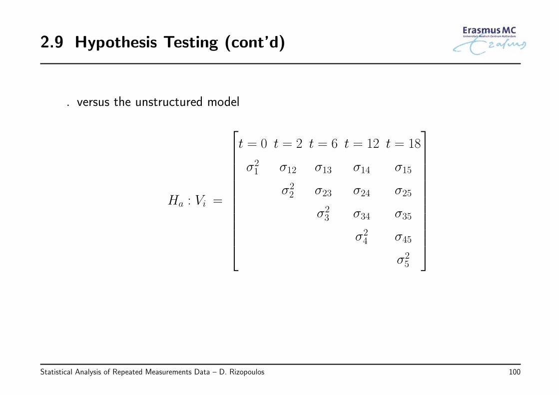
◃ versus the unstructured model
Ha : Vi =
t = 0 t = 2 t = 6 t = 12 t = 18
σ21 σ12 σ13 σ14 σ15
σ22 σ23 σ24 σ25
σ23 σ34 σ35
σ24 σ45
σ25
Statistical Analysis of Repeated Measurements Data – D. Rizopoulos 100
2.9 Hypothesis Testing (cont’d)
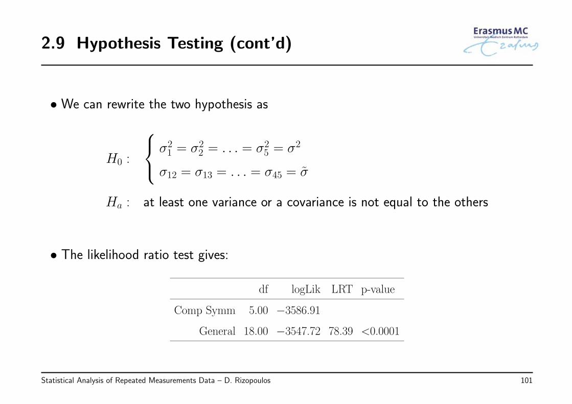
• We can rewrite the two hypothesis as
H0 :
σ21 = σ2
2 = . . . = σ25 = σ2
σ12 = σ13 = . . . = σ45 = σ
Ha : at least one variance or a covariance is not equal to the others
• The likelihood ratio test gives:
df logLik LRT p-value
Comp Symm 5.00 −3586.91
General 18.00 −3547.72 78.39 <0.0001
Statistical Analysis of Repeated Measurements Data – D. Rizopoulos 101
2.9 Hypothesis Testing (cont’d)
• When we have non-nested models we cannot use standard tests anymore
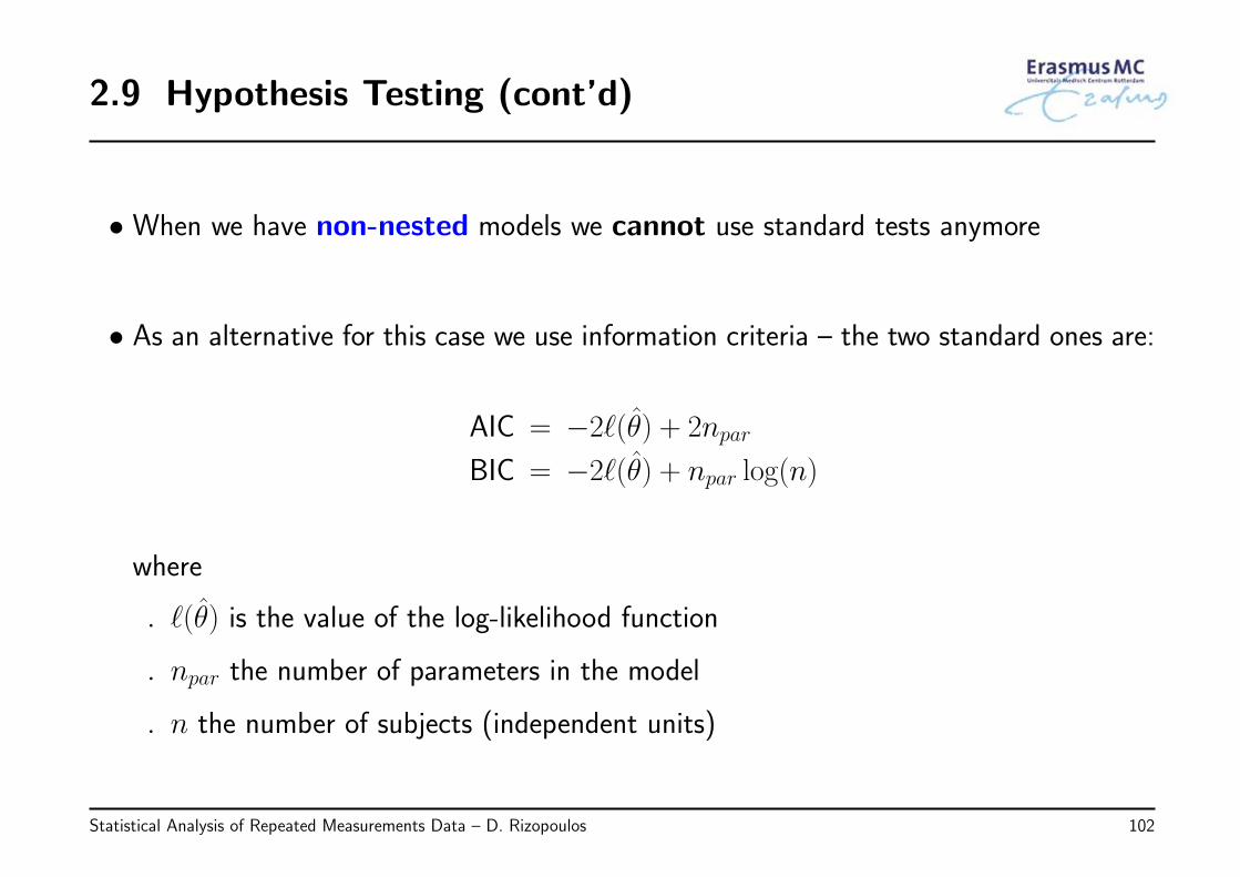
• As an alternative for this case we use information criteria – the two standard ones are:
AIC = −2ℓ(θ) + 2npar
BIC = −2ℓ(θ) + npar log(n)
where
◃ ℓ(θ) is the value of the log-likelihood function
◃ npar the number of parameters in the model
◃ n the number of subjects (independent units)
Statistical Analysis of Repeated Measurements Data – D. Rizopoulos 102
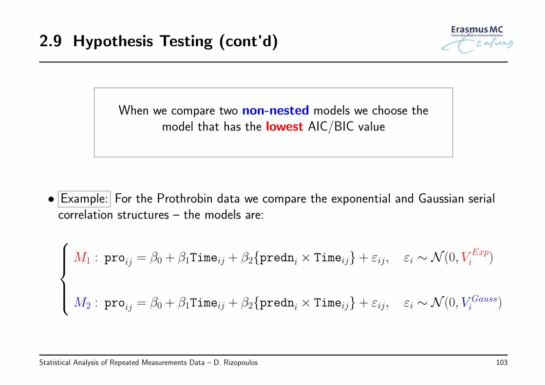
2.9 Hypothesis Testing (cont’d)
When we compare two non-nested models we choose themodel that has the lowest AIC/BIC value
• Example: For the Prothrobin data we compare the exponential and Gaussian serialcorrelation structures – the models are:
M1 : proij = β0 + β1Timeij + β2{predni × Timeij} + εij, εi ∼ N (0, V Expi )
M2 : proij = β0 + β1Timeij + β2{predni × Timeij} + εij, εi ∼ N (0, V Gaussi )
Statistical Analysis of Repeated Measurements Data – D. Rizopoulos 103
2.9 Hypothesis Testing (cont’d)
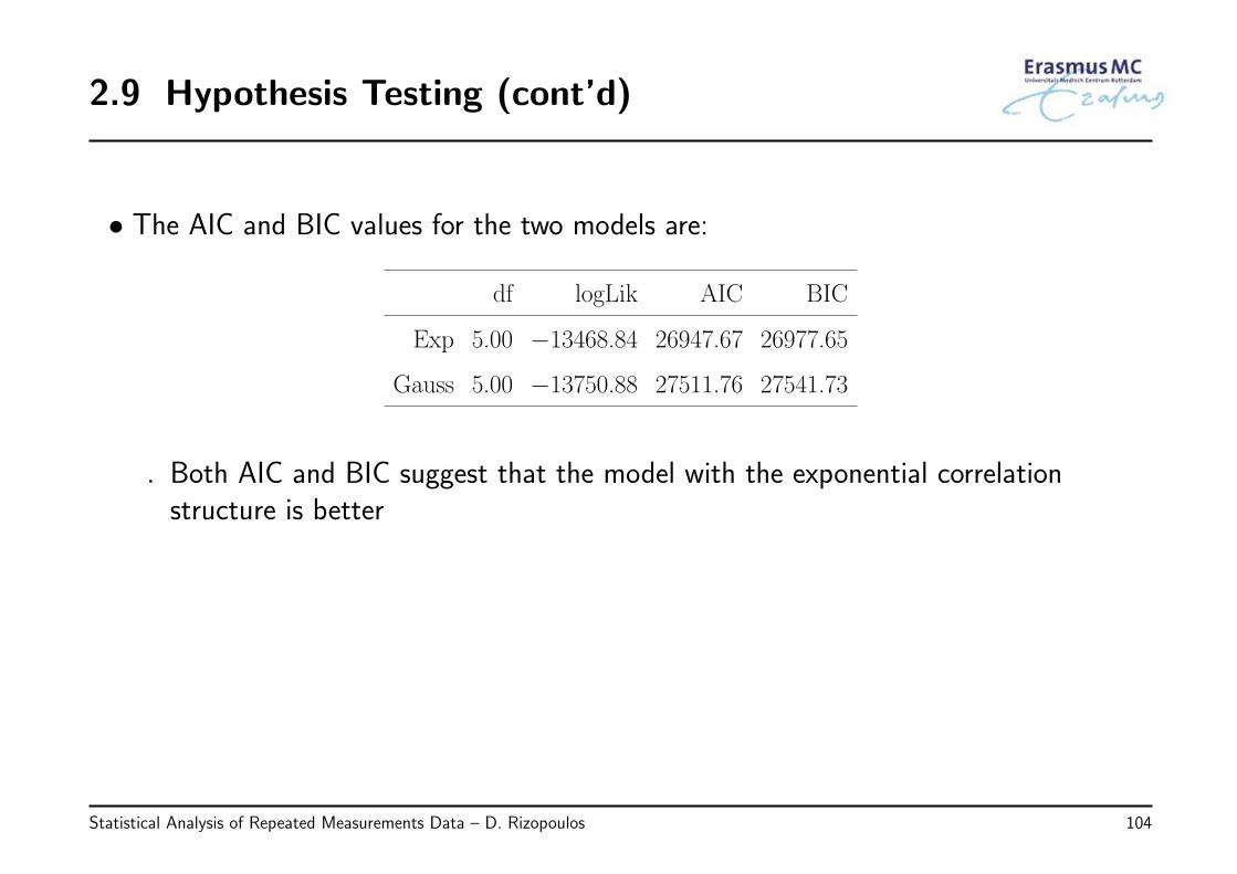
• The AIC and BIC values for the two models are:
df logLik AIC BIC
Exp 5.00 −13468.84 26947.67 26977.65
Gauss 5.00 −13750.88 27511.76 27541.73
◃ Both AIC and BIC suggest that the model with the exponential correlationstructure is better
Statistical Analysis of Repeated Measurements Data – D. Rizopoulos 104
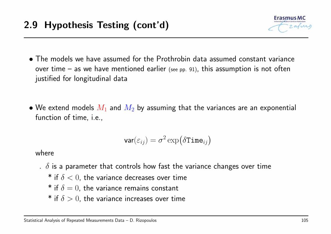
2.9 Hypothesis Testing (cont’d)
• The models we have assumed for the Prothrobin data assumed constant varianceover time – as we have mentioned earlier (see pp. 91), this assumption is not oftenjustified for longitudinal data
• We extend models M1 and M2 by assuming that the variances are an exponentialfunction of time, i.e.,
var(εij) = σ2 exp(δTimeij
)where
◃ δ is a parameter that controls how fast the variance changes over time
* if δ < 0, the variance decreases over time
* if δ = 0, the variance remains constant
* if δ > 0, the variance increases over time
Statistical Analysis of Repeated Measurements Data – D. Rizopoulos 105
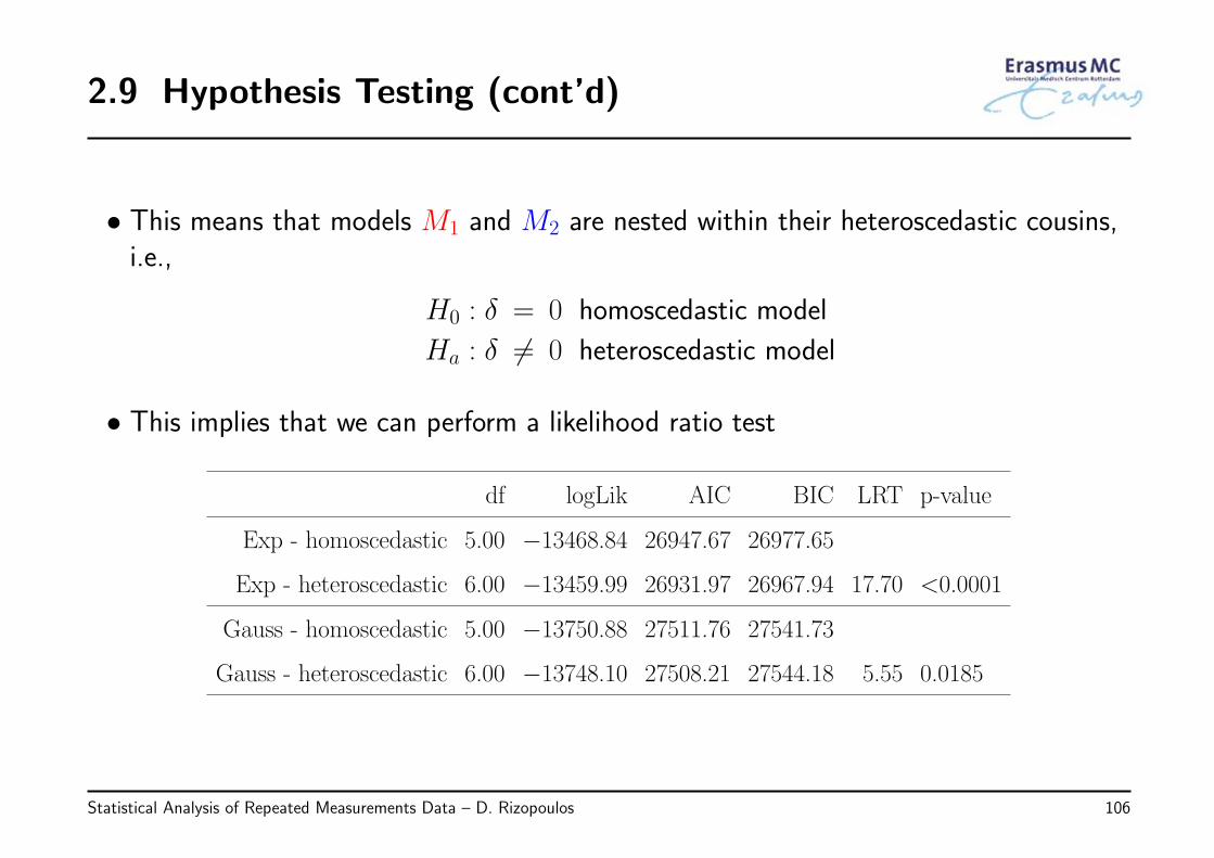
2.9 Hypothesis Testing (cont’d)
• This means that models M1 and M2 are nested within their heteroscedastic cousins,i.e.,
H0 : δ = 0 homoscedastic model
Ha : δ = 0 heteroscedastic model
• This implies that we can perform a likelihood ratio test
df logLik AIC BIC LRT p-value
Exp - homoscedastic 5.00 −13468.84 26947.67 26977.65
Exp - heteroscedastic 6.00 −13459.99 26931.97 26967.94 17.70 <0.0001
Gauss - homoscedastic 5.00 −13750.88 27511.76 27541.73
Gauss - heteroscedastic 6.00 −13748.10 27508.21 27544.18 5.55 0.0185
Statistical Analysis of Repeated Measurements Data – D. Rizopoulos 106
2.9 Hypothesis Testing (cont’d)
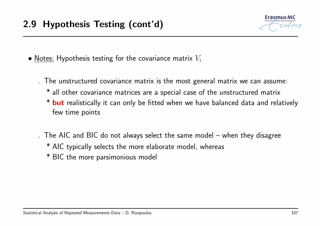
• Notes: Hypothesis testing for the covariance matrix Vi
◃ The unstructured covariance matrix is the most general matrix we can assume:
* all other covariance matrices are a special case of the unstructured matrix
* but realistically it can only be fitted when we have balanced data and relativelyfew time points
◃ The AIC and BIC do not always select the same model – when they disagree
* AIC typically selects the more elaborate model, whereas
* BIC the more parsimonious model
Statistical Analysis of Repeated Measurements Data – D. Rizopoulos 107
2.9 Hypothesis Testing (cont’d)
• Hypothesis testing for the regression coefficients β: We assume that first asuitable choice for the covariance matrix has been made
• In the majority of the cases we compare nested models, and hence standard tests canbe used
• We distinguish between two cases
◃ tests for individual coefficients
◃ tests for groups of coefficients
Statistical Analysis of Repeated Measurements Data – D. Rizopoulos 108
2.9 Hypothesis Testing (cont’d)
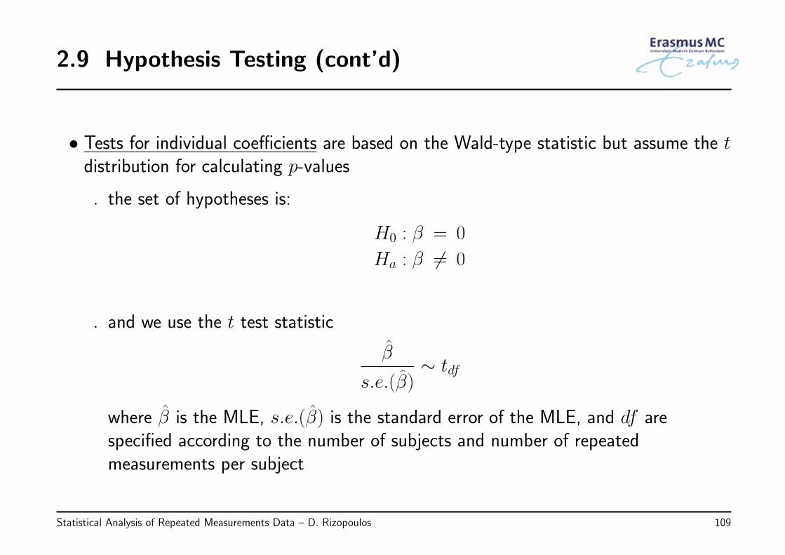
• Tests for individual coefficients are based on the Wald-type statistic but assume the tdistribution for calculating p-values
◃ the set of hypotheses is:
H0 : β = 0
Ha : β = 0
◃ and we use the t test statistic
β
s.e.(β)∼ tdf
where β is the MLE, s.e.(β) is the standard error of the MLE, and df arespecified according to the number of subjects and number of repeatedmeasurements per subject
Statistical Analysis of Repeated Measurements Data – D. Rizopoulos 109
2.9 Hypothesis Testing (cont’d)
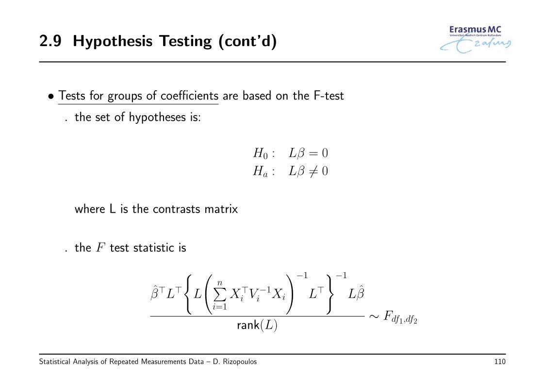
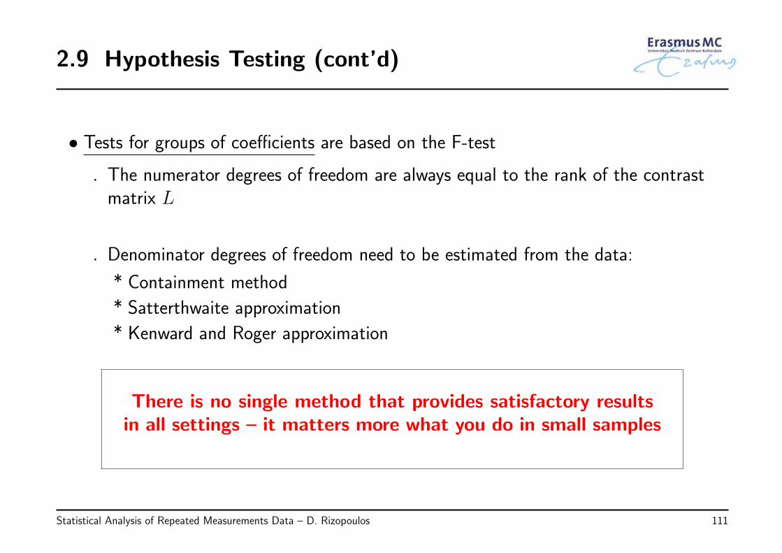
• Tests for groups of coefficients are based on the F-test
◃ the set of hypotheses is:
H0 : Lβ = 0
Ha : Lβ = 0
where L is the contrasts matrix
◃ the F test statistic is
β⊤L⊤
{L
(n∑
i=1
X⊤i V
−1i Xi
)−1
L⊤
}−1
Lβ
rank(L)∼ Fdf1,df2
Statistical Analysis of Repeated Measurements Data – D. Rizopoulos 110
2.9 Hypothesis Testing (cont’d)
• Tests for groups of coefficients are based on the F-test
◃ The numerator degrees of freedom are always equal to the rank of the contrastmatrix L
◃ Denominator degrees of freedom need to be estimated from the data:
* Containment method
* Satterthwaite approximation
* Kenward and Roger approximation
There is no single method that provides satisfactory resultsin all settings – it matters more what you do in small samples
Statistical Analysis of Repeated Measurements Data – D. Rizopoulos 111
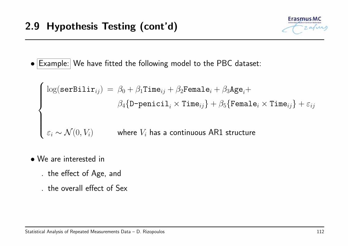
2.9 Hypothesis Testing (cont’d)
• Example: We have fitted the following model to the PBC dataset:
log(serBilirij) = β0 + β1Timeij + β2Femalei + β3Agei+
β4{D-penicili × Timeij} + β5{Femalei × Timeij} + εij
εi ∼ N (0, Vi) where Vi has a continuous AR1 structure
• We are interested in
◃ the effect of Age, and
◃ the overall effect of Sex
Statistical Analysis of Repeated Measurements Data – D. Rizopoulos 112
2.9 Hypothesis Testing (cont’d)
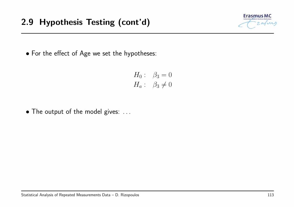
• For the effect of Age we set the hypotheses:
H0 : β3 = 0
Ha : β3 = 0
• The output of the model gives: . . .
Statistical Analysis of Repeated Measurements Data – D. Rizopoulos 113
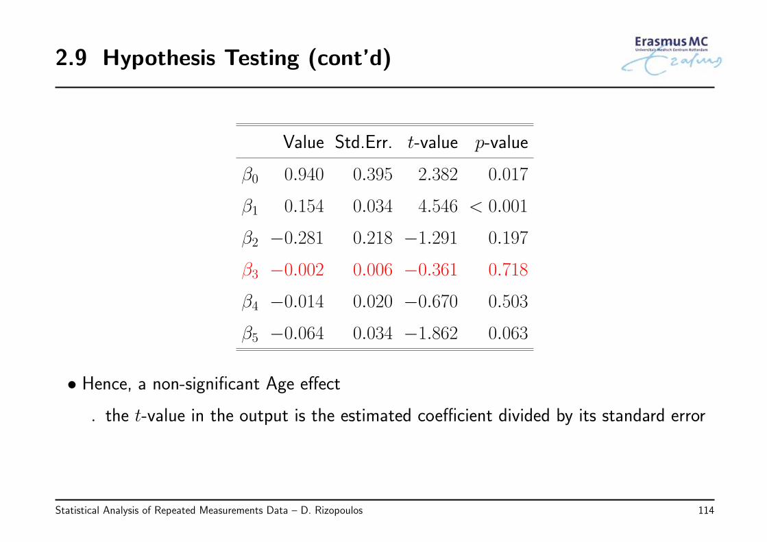
2.9 Hypothesis Testing (cont’d)
Value Std.Err. t-value p-value
β0 0.940 0.395 2.382 0.017
β1 0.154 0.034 4.546 < 0.001
β2 −0.281 0.218 −1.291 0.197
β3 −0.002 0.006 −0.361 0.718
β4 −0.014 0.020 −0.670 0.503
β5 −0.064 0.034 −1.862 0.063
• Hence, a non-significant Age effect
◃ the t-value in the output is the estimated coefficient divided by its standard error
Statistical Analysis of Repeated Measurements Data – D. Rizopoulos 114
2.9 Hypothesis Testing (cont’d)
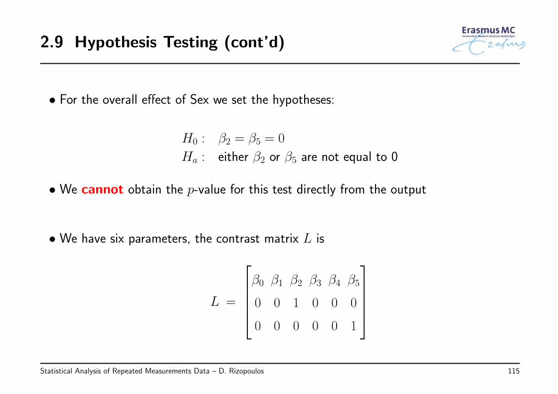
• For the overall effect of Sex we set the hypotheses:
H0 : β2 = β5 = 0
Ha : either β2 or β5 are not equal to 0
• We cannot obtain the p-value for this test directly from the output
• We have six parameters, the contrast matrix L is
L =
β0 β1 β2 β3 β4 β5
0 0 1 0 0 0
0 0 0 0 0 1
Statistical Analysis of Repeated Measurements Data – D. Rizopoulos 115
2.9 Hypothesis Testing (cont’d)
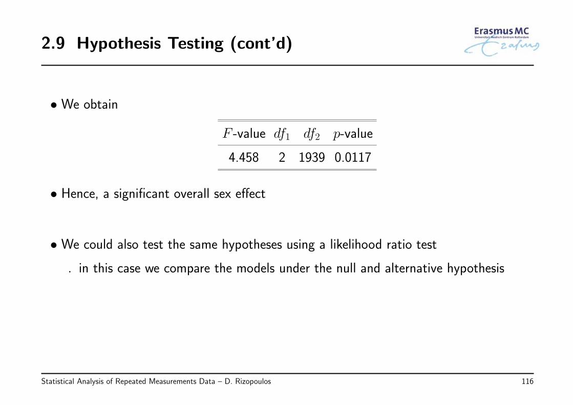
• We obtain
F -value df1 df2 p-value
4.458 2 1939 0.0117
• Hence, a significant overall sex effect
• We could also test the same hypotheses using a likelihood ratio test
◃ in this case we compare the models under the null and alternative hypothesis
Statistical Analysis of Repeated Measurements Data – D. Rizopoulos 116
2.9 Hypothesis Testing (cont’d)
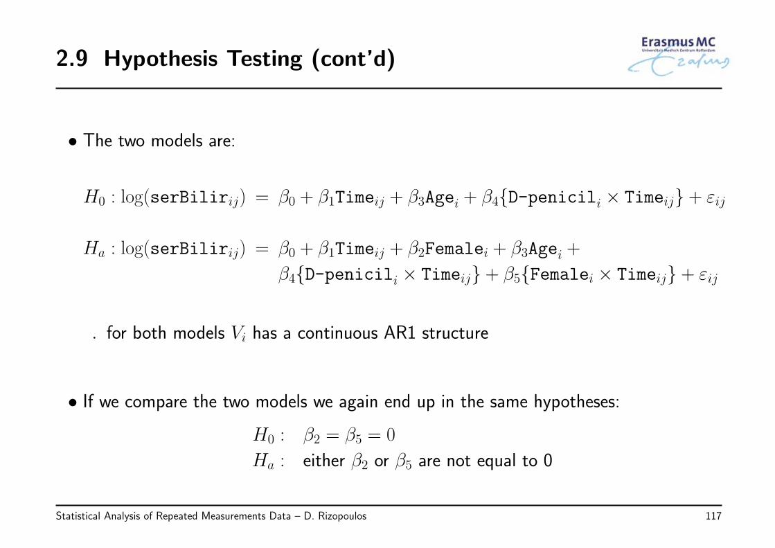
• The two models are:
H0 : log(serBilirij) = β0 + β1Timeij + β3Agei + β4{D-penicili × Timeij} + εij
Ha : log(serBilirij) = β0 + β1Timeij + β2Femalei + β3Agei +
β4{D-penicili × Timeij} + β5{Femalei × Timeij} + εij
◃ for both models Vi has a continuous AR1 structure
• If we compare the two models we again end up in the same hypotheses:
H0 : β2 = β5 = 0
Ha : either β2 or β5 are not equal to 0
Statistical Analysis of Repeated Measurements Data – D. Rizopoulos 117
2.9 Hypothesis Testing (cont’d)
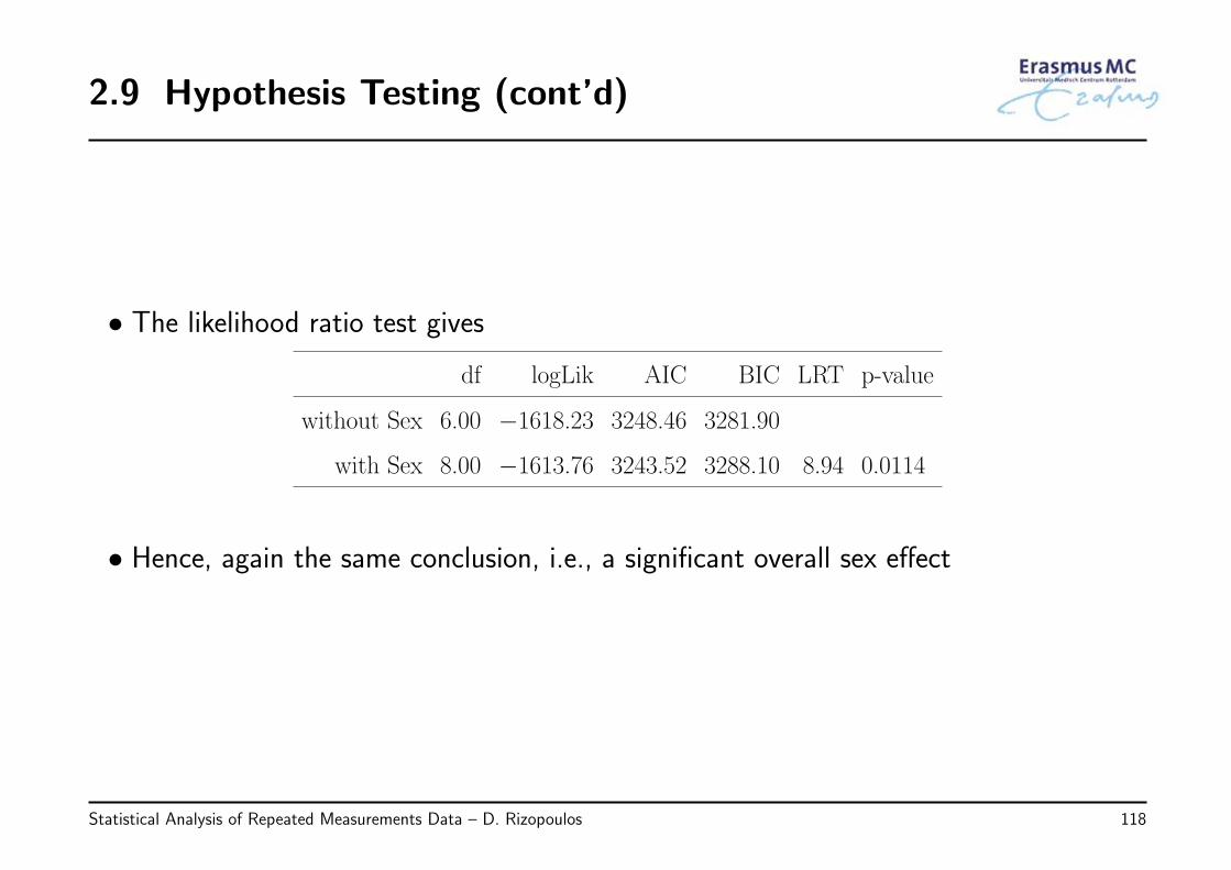
• The likelihood ratio test gives
df logLik AIC BIC LRT p-value
without Sex 6.00 −1618.23 3248.46 3281.90
with Sex 8.00 −1613.76 3243.52 3288.10 8.94 0.0114
• Hence, again the same conclusion, i.e., a significant overall sex effect
Statistical Analysis of Repeated Measurements Data – D. Rizopoulos 118
2.9 Hypothesis Testing (cont’d)
• Notes: Hypothesis testing for the regression coefficients β
◃ The likelihood ratio test, and the classical univariate and multivariate Wald tests(i.e., using the χ2 distribution instead of the t or F distributions) are ‘liberal’
* they give smaller p-values than the ones they should give, especially in smallsamples
◃ Important: The likelihood ratio test for comparing models with different Xβparts is only valid when the models have been fitted using maximum likelihoodand not REML (see also pp. 73–77)
Statistical Analysis of Repeated Measurements Data – D. Rizopoulos 119
2.10 Confidence Intervals
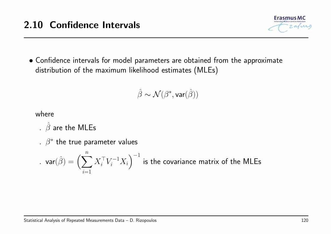
• Confidence intervals for model parameters are obtained from the approximatedistribution of the maximum likelihood estimates (MLEs)
β ∼ N (β∗, var(β))
where
◃ β are the MLEs
◃ β∗ the true parameter values
◃ var(β) =( n∑
i=1
X⊤i V
−1i Xi
)−1
is the covariance matrix of the MLEs
Statistical Analysis of Repeated Measurements Data – D. Rizopoulos 120
2.10 Confidence Intervals (cont’d)
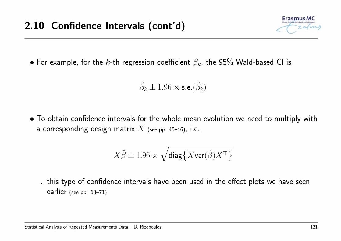
• For example, for the k-th regression coefficient βk, the 95% Wald-based CI is
βk ± 1.96× s.e.(βk)
• To obtain confidence intervals for the whole mean evolution we need to multiply witha corresponding design matrix X (see pp. 45–46), i.e.,
Xβ ± 1.96×√diag
{Xvar(β)X⊤
}◃ this type of confidence intervals have been used in the effect plots we have seenearlier (see pp. 68–71)
Statistical Analysis of Repeated Measurements Data – D. Rizopoulos 121
2.11 Design Considerations - Sample Size
• Two interrelated questions relevant to hypothesis testing are how to perform power& sample size calculations
◃ power: is the probability that we will find a statistically significant differencebetween the two groups, given that this difference truly exists
◃ sample size: in the design phase of a study, and for a given a priori postulatedsetting, we often want to find how many subjects we need to enrol to detect thedifference of interest, with a prespecified level of power (and a prespecifiedsignificance level)
Statistical Analysis of Repeated Measurements Data – D. Rizopoulos 122
2.11 Design Considerations - Sample Size (cont’d)
• In the literature several formulas for sample size calculations have been developed formarginal and linear mixed models (see Chapter 3)
• However, in the majority of the cases these formulas are only applicable in simplesettings, and cannot account for common features of longitudinal data, e.g.,
◃ complex correlation structures
◃ unbalanced data
◃ missing data (see Chapter 6)
Statistical Analysis of Repeated Measurements Data – D. Rizopoulos 123
2.11 Design Considerations - Sample Size (cont’d)
• The only viable and trustworthy approach is to use simulationThis entails the following generic steps
S1: Simulate longitudinal responses under the postulated model, and a specificsample size n
* in this step the covariates could be set fixed or also simulated
S2: Fit the postulated model in the simulated data
S3: Perform the hypothesis test of interest and retain the p-value
Statistical Analysis of Repeated Measurements Data – D. Rizopoulos 124
2.11 Design Considerations - Sample Size (cont’d)
• Repeat Steps 1–3 M times (e.g., M = 500 or M = 1000), and calculate how manytimes the p-value was significant at significance level α (e.g., α = 0.05)
◃ the percentage of times the test was significant is the estimated power for thespecific setting under consideration
Statistical Analysis of Repeated Measurements Data – D. Rizopoulos 125
2.11 Design Considerations - Sample Size (cont’d)
• Notes: On power calculation for repeated measurement models
◃ To perform a sample size calculation we just repeat the above simulationprocedure with increasing n until the power reaches the prespecified level
◃ The simulation approach allows very easily to investigate how power is affected byspecific changes in the design, e.g.,
* increasing the number of repeated measurements per subject ni versusincreasing the number of subjects n
* different percentages of missing data
* . . .
◃ The downside is that each time a new syntax needs to be written to do thesecalculations
Statistical Analysis of Repeated Measurements Data – D. Rizopoulos 126
2.12 Residuals
All statistical models are based on assumptions
• Hence, to extract meaningful conclusions we need to check whether theseassumptions are (crudely) violated
Statistical Analysis of Repeated Measurements Data – D. Rizopoulos 127
2.12 Residuals (cont’d)
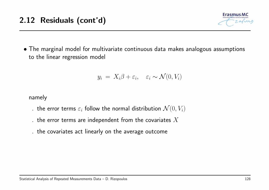
• The marginal model for multivariate continuous data makes analogous assumptionsto the linear regression model
yi = Xiβ + εi, εi ∼ N (0, Vi)
namely
◃ the error terms εi follow the normal distribution N (0, Vi)
◃ the error terms are independent from the covariates X
◃ the covariates act linearly on the average outcome
Statistical Analysis of Repeated Measurements Data – D. Rizopoulos 128
2.12 Residuals (cont’d)
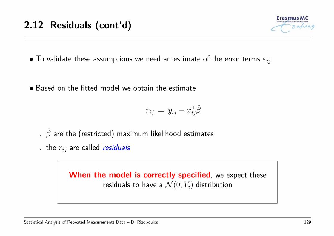
• To validate these assumptions we need an estimate of the error terms εij
• Based on the fitted model we obtain the estimate
rij = yij − x⊤ijβ
◃ β are the (restricted) maximum likelihood estimates
◃ the rij are called residuals
When the model is correctly specified, we expect theseresiduals to have a N (0, Vi) distribution
Statistical Analysis of Repeated Measurements Data – D. Rizopoulos 129
2.12 Residuals (cont’d)
• Hence, we expect these residuals to be correlated and possibly also heteroscedastic
◃ ‘heteroscedastic’ means that they exhibit non-constant variance
• This feature complicates matters because it is not easy to assess if the residualsexhibit the assumed properties
• To overcome this problem we need to transform rij to a scale that has easier tocheck properties
◃ for example, in general, it is easier to assess whether a particular variable has astandard normal distribution
Statistical Analysis of Repeated Measurements Data – D. Rizopoulos 130
2.12 Residuals (cont’d)
• To achieve this we multiply the residual with the inverse Choleski factor
rnormi = H−1i ri = H−1
i (yi −Xiβ)
where
◃ Hi is an upper-triangular matrix with the property H⊤i Hi = Vi, with Vi denoting
the estimated covariance matrix
◃ rnormij are called normalized residuals and when the covariance matrix is correctlyspecified, they should be approximately distributed as N (0, 1) random variables
Statistical Analysis of Repeated Measurements Data – D. Rizopoulos 131
2.12 Residuals (cont’d)
• When we have assumed a homoscedastic covariance matrix (i.e., variance remainsconstant), another transformation that it is often used is
rPearsi = σ−1ri = σ−1(yi −Xiβ)
where
◃ σ denotes the estimated standard deviation of the error term, i.e., Vi has thestructure σ2Ri, with Ri denoting a correlation matrix
◃ rPearsij are called Pearson residuals and when the covariance matrix is correctlyspecified, they should be approximately distributed as N (0, Ri) random variables
Statistical Analysis of Repeated Measurements Data – D. Rizopoulos 132
2.12 Residuals (cont’d)
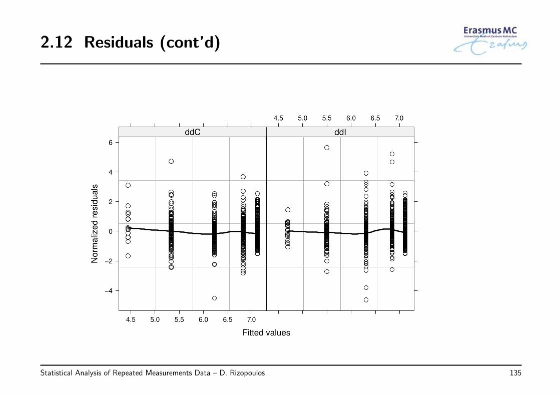
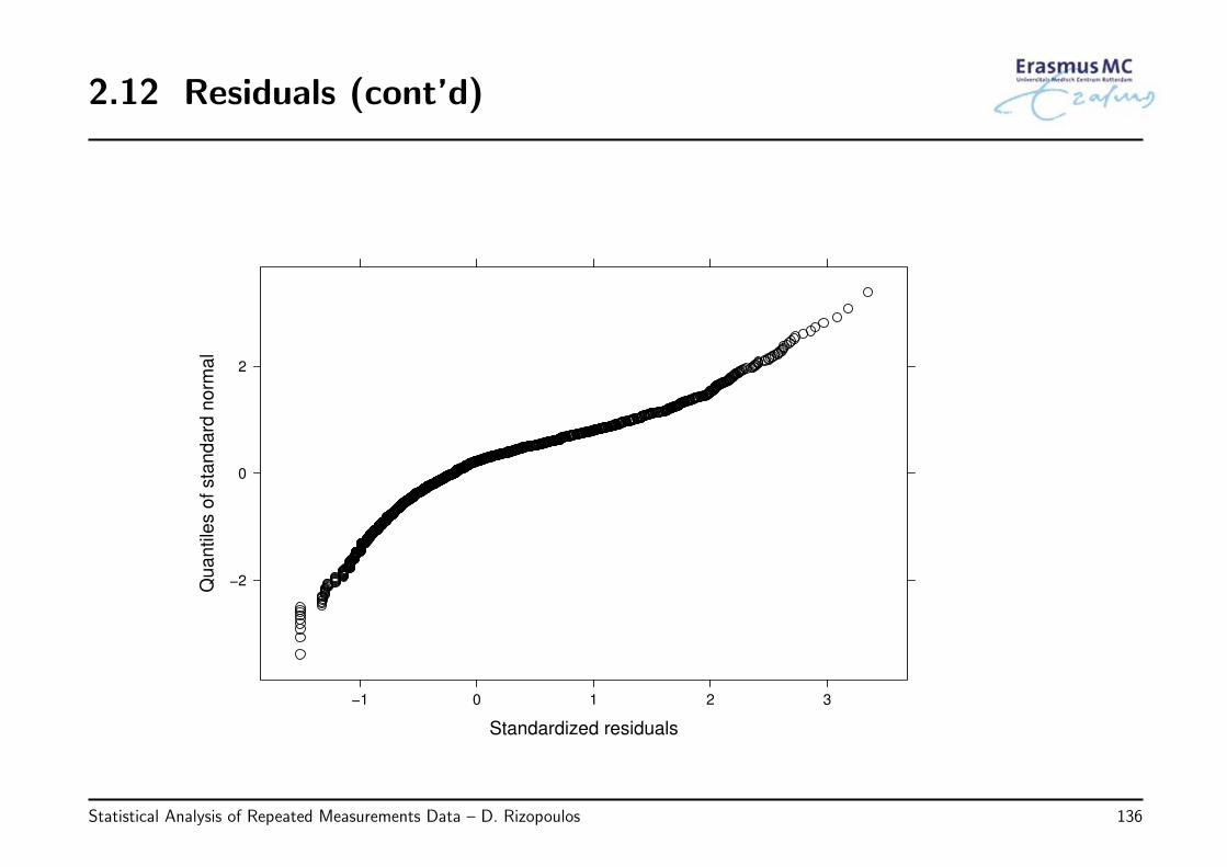
• Example: We evaluate the assumptions behind the following model fitted to theAIDS dataset:
√CD4ij = β0 + β1Timeij + β2{ddIi × Timeij} + εij,
εi ∼ N (0, Vi), Vi is unstructured
by plotting
◃ the standardized residuals versus fitted values
◃ the normalized residuals versus fitted values per treatment group
◃ QQ-plot of the standardized residuals
Statistical Analysis of Repeated Measurements Data – D. Rizopoulos 133
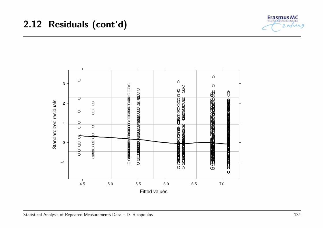
2.12 Residuals (cont’d)
Fitted values
Sta
nd
ard
ized
resid
ua
ls
−1
0
1
2
3
4.5 5.0 5.5 6.0 6.5 7.0
Statistical Analysis of Repeated Measurements Data – D. Rizopoulos 134
2.12 Residuals (cont’d)
Fitted values
No
rma
lize
d r
esid
ua
ls
−4
−2
0
2
4
6
4.5 5.0 5.5 6.0 6.5 7.0
ddC
4.5 5.0 5.5 6.0 6.5 7.0
ddI
Statistical Analysis of Repeated Measurements Data – D. Rizopoulos 135
2.12 Residuals (cont’d)
Standardized residuals
Qu
an
tile
s o
f sta
nda
rd n
orm
al
−2
0
2
−1 0 1 2 3
Statistical Analysis of Repeated Measurements Data – D. Rizopoulos 136
2.12 Residuals (cont’d)
• Observations
◃ the plots of the residuals versus the fitted values do show a slightly systematicbehavior with more positive residuals in the range of low fitted values
◃ the QQ-plot is not perfect, but does not show a big discrepancy from normality
Statistical Analysis of Repeated Measurements Data – D. Rizopoulos 137
2.12 Residuals (cont’d)
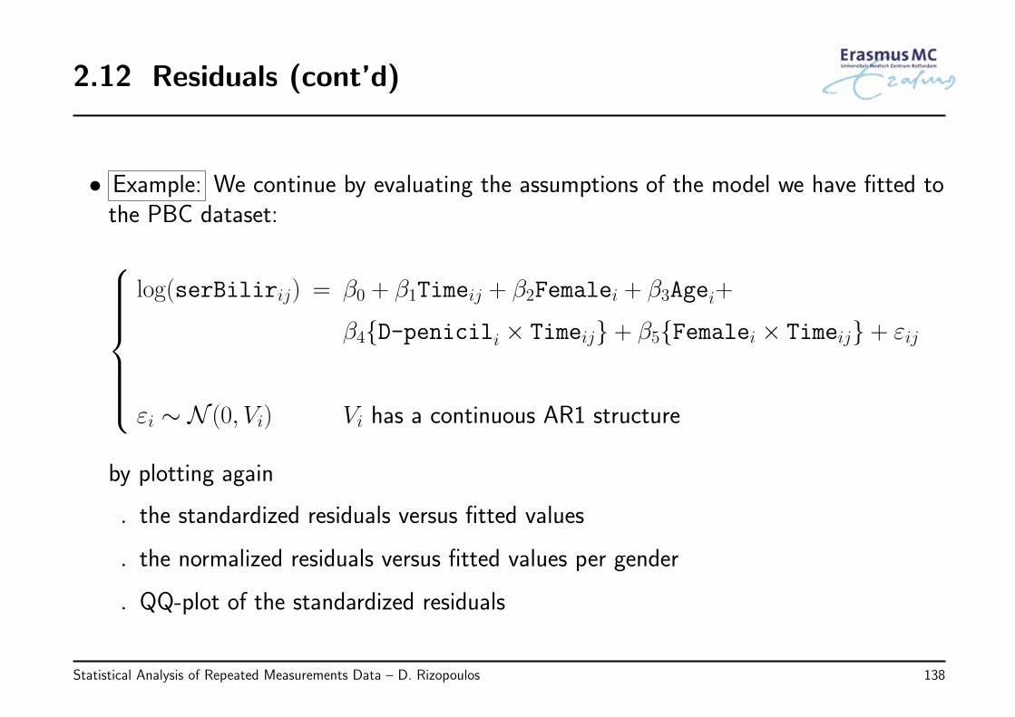
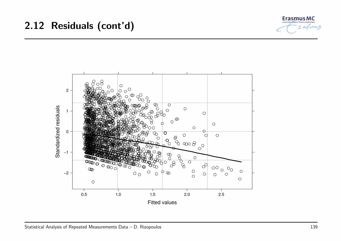
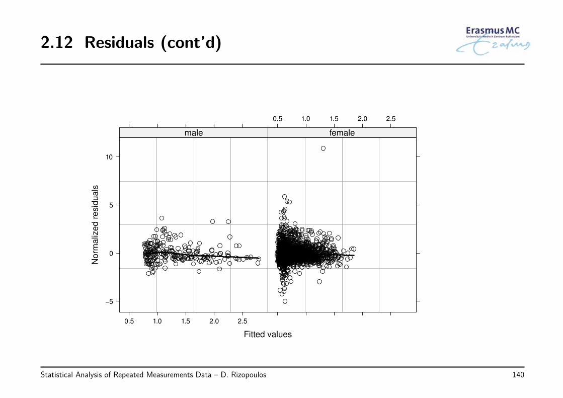
• Example: We continue by evaluating the assumptions of the model we have fitted tothe PBC dataset:
log(serBilirij) = β0 + β1Timeij + β2Femalei + β3Agei+
β4{D-penicili × Timeij} + β5{Femalei × Timeij} + εij
εi ∼ N (0, Vi) Vi has a continuous AR1 structure
by plotting again
◃ the standardized residuals versus fitted values
◃ the normalized residuals versus fitted values per gender
◃ QQ-plot of the standardized residuals
Statistical Analysis of Repeated Measurements Data – D. Rizopoulos 138
2.12 Residuals (cont’d)
Fitted values
Sta
nd
ard
ized
resid
ua
ls
−2
−1
0
1
2
0.5 1.0 1.5 2.0 2.5
Statistical Analysis of Repeated Measurements Data – D. Rizopoulos 139
2.12 Residuals (cont’d)
Fitted values
No
rma
lize
d r
esid
ua
ls
−5
0
5
10
0.5 1.0 1.5 2.0 2.5
male
0.5 1.0 1.5 2.0 2.5
female
Statistical Analysis of Repeated Measurements Data – D. Rizopoulos 140
2.12 Residuals (cont’d)
Standardized residuals
Qu
an
tile
s o
f sta
nda
rd n
orm
al
−2
0
2
−2 −1 0 1 2
Statistical Analysis of Repeated Measurements Data – D. Rizopoulos 141
2.12 Residuals (cont’d)
• Observations
◃ the plot of the standardized residuals versus fitted values shows a clear systematictrend with more negative residuals in the range of high fitted values
◃ the plot of normalized residuals versus fitted values shows an outlying observationfor female and some slight heteroscedasticity (higher spread of residuals for lowfitted values than for high)
◃ the QQ-plot suggests a good fit of the normal distribution
Statistical Analysis of Repeated Measurements Data – D. Rizopoulos 142
2.13 Review of Key Points
• Methods for analyzing grouped/correlated data
◃ naive approaches working on parts or summaries of the data ⇒ loss of information
◃ marginal models ⇒ extension of simple linear regression to the context ofcorrelated data
• Marginal models: Features
◃ error terms are assumed correlated ⇒ we need to make an appropriate assumption
◃ mean structure is build as in standard regression models – however, need toaccount for potential nonlinear effects of time and/or interaction terms
◃ model building: we start from a ‘fully’ specified mean structure, we select anappropriate covariance structure, and then we return to make inference for themean structure
Statistical Analysis of Repeated Measurements Data – D. Rizopoulos 143
2.13 Review of Key Points (cont’d)
• Hypothesis testing
◃ for the covariance structure and for nested models likelihood ratio tests are mostoften used, for non-nested models AIC/BIC
◃ for the mean structure t and F tests with appropriate degrees of freedom
• Residuals
◃ standard residuals plots are used to check the model assumptions
◃ standardized and normalized residuals
Statistical Analysis of Repeated Measurements Data – D. Rizopoulos 144
Chapter 3
The Linear Mixed Effects Model
Statistical Analysis of Repeated Measurements Data – D. Rizopoulos 145
3.1 The Linear Mixed Model
• In the previous chapter we focused on the multivariate regression model
yi = Xiβ + εi, εi ∼ N (0, Vi),
where
◃ yi the vector of responses for the ith subject
◃ Xi design matrix describing structural component
◃ Vi covariance matrix describing the correlation structure
Statistical Analysis of Repeated Measurements Data – D. Rizopoulos 146
3.1 The Linear Mixed Model (cont’d)
• Alternative intuitive approach: Each subject in the population has her ownsubject-specific mean response profile over time
Statistical Analysis of Repeated Measurements Data – D. Rizopoulos 147
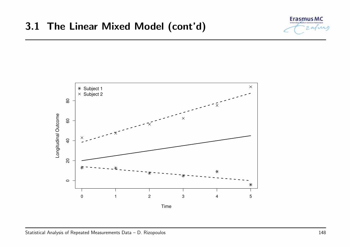
3.1 The Linear Mixed Model (cont’d)
0 1 2 3 4 5
02
04
06
08
0
Time
Longitudin
al O
utc
om
e
Subject 1
Subject 2
Statistical Analysis of Repeated Measurements Data – D. Rizopoulos 148
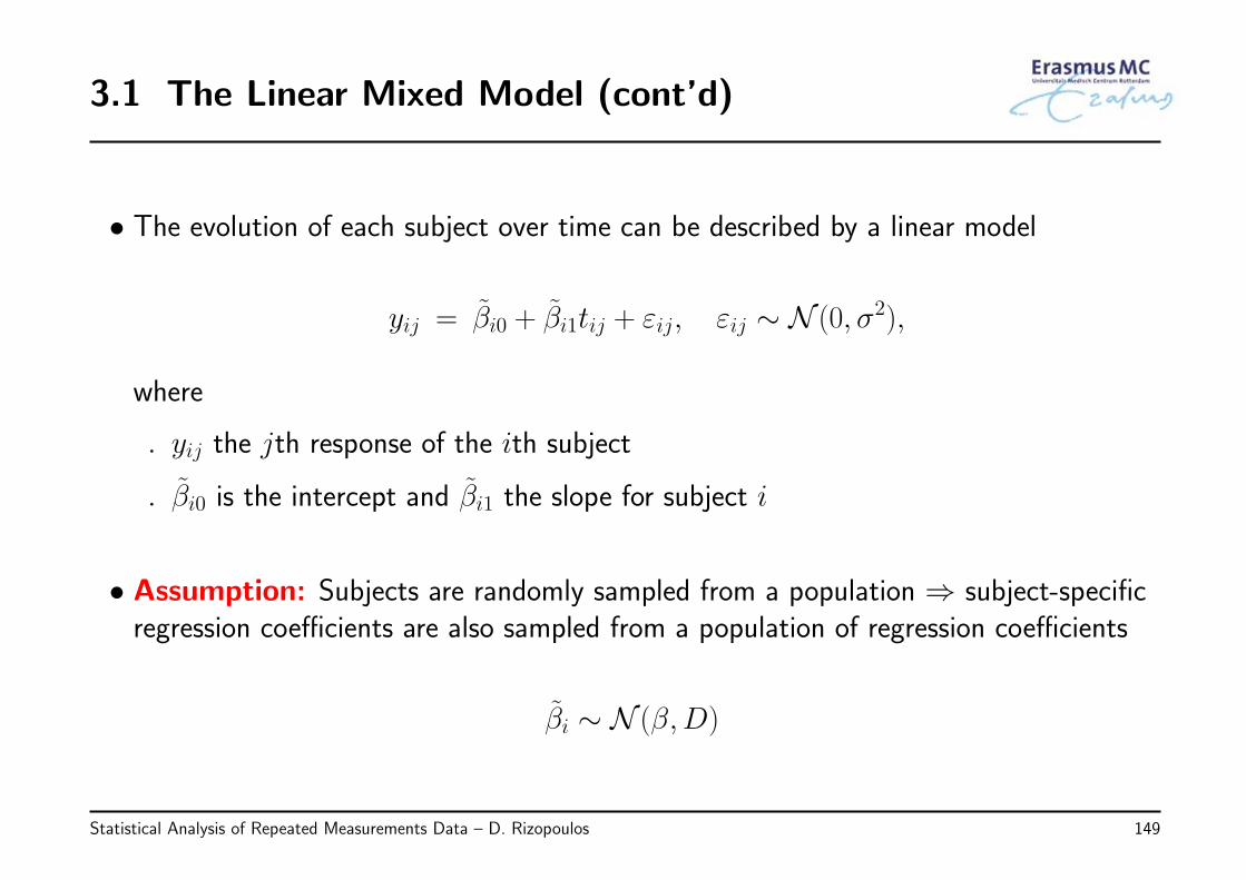
3.1 The Linear Mixed Model (cont’d)
• The evolution of each subject over time can be described by a linear model
yij = βi0 + βi1tij + εij, εij ∼ N (0, σ2),
where
◃ yij the jth response of the ith subject
◃ βi0 is the intercept and βi1 the slope for subject i
• Assumption: Subjects are randomly sampled from a population ⇒ subject-specificregression coefficients are also sampled from a population of regression coefficients
βi ∼ N (β,D)
Statistical Analysis of Repeated Measurements Data – D. Rizopoulos 149
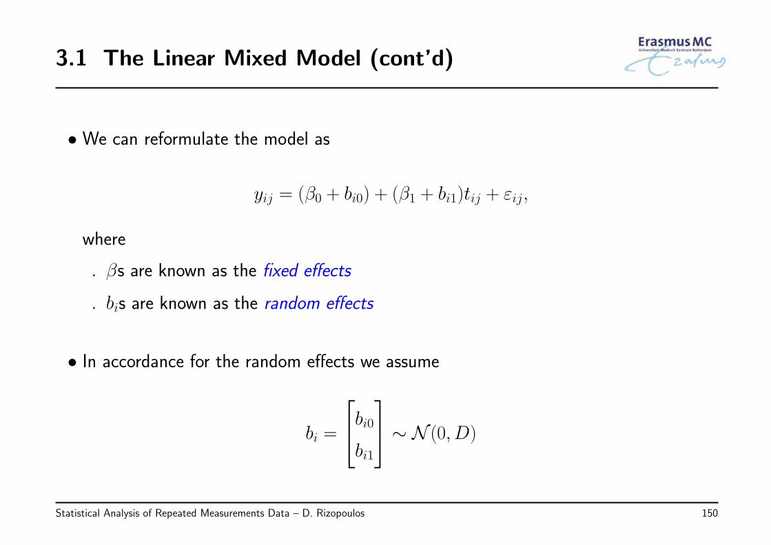
3.1 The Linear Mixed Model (cont’d)
• We can reformulate the model as
yij = (β0 + bi0) + (β1 + bi1)tij + εij,
where
◃ βs are known as the fixed effects
◃ bis are known as the random effects
• In accordance for the random effects we assume
bi =
bi0bi1
∼ N (0, D)
Statistical Analysis of Repeated Measurements Data – D. Rizopoulos 150
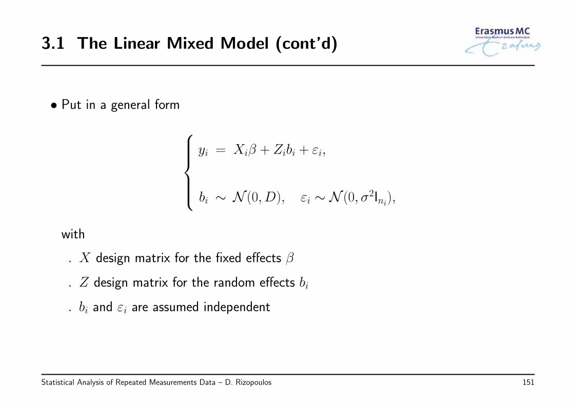
3.1 The Linear Mixed Model (cont’d)
• Put in a general formyi = Xiβ + Zibi + εi,
bi ∼ N (0, D), εi ∼ N (0, σ2Ini),
with
◃ X design matrix for the fixed effects β
◃ Z design matrix for the random effects bi
◃ bi and εi are assumed independent
Statistical Analysis of Repeated Measurements Data – D. Rizopoulos 151
3.2 Interpretation
• Fixed and random effects:
◃ βj denotes the change in the average yi when xj is increased by one unit
◃ bi are interpreted in terms of how a subset of the regression parameters for the ithsubject deviates from those in the population
• Advantageous feature: population + subject-specific predictions
◃ β describes mean response changes in the population
◃ β + bi describes individual response trajectories
Statistical Analysis of Repeated Measurements Data – D. Rizopoulos 152
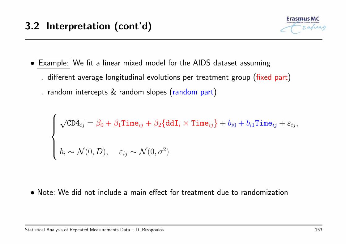
3.2 Interpretation (cont’d)
• Example: We fit a linear mixed model for the AIDS dataset assuming
◃ different average longitudinal evolutions per treatment group (fixed part)
◃ random intercepts & random slopes (random part)
√CD4ij = β0 + β1Timeij + β2{ddIi × Timeij} + bi0 + bi1Timeij + εij,
bi ∼ N (0, D), εij ∼ N (0, σ2)
• Note: We did not include a main effect for treatment due to randomization
Statistical Analysis of Repeated Measurements Data – D. Rizopoulos 153
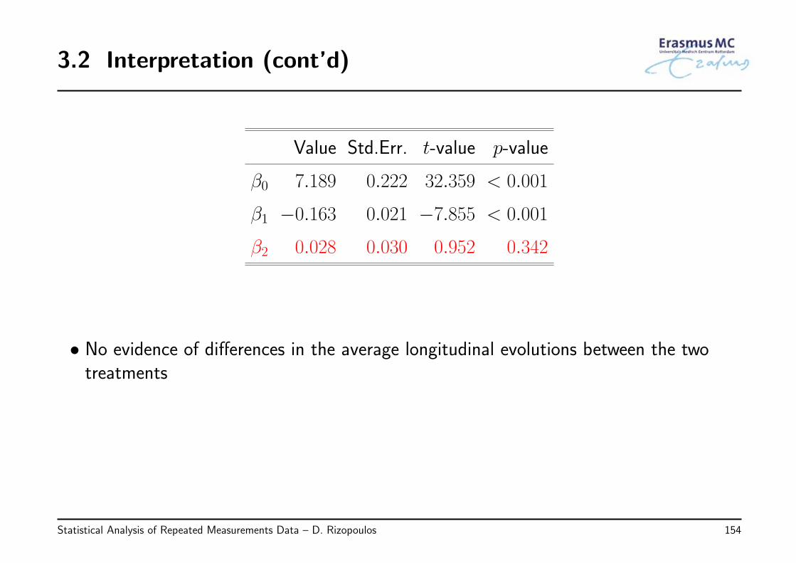
3.2 Interpretation (cont’d)
Value Std.Err. t-value p-value
β0 7.189 0.222 32.359 < 0.001
β1 −0.163 0.021 −7.855 < 0.001
β2 0.028 0.030 0.952 0.342
• No evidence of differences in the average longitudinal evolutions between the twotreatments
Statistical Analysis of Repeated Measurements Data – D. Rizopoulos 154
3.2 Interpretation (cont’d)
• Interaction & nonlinear terms: As we have seen in the previous chapter (see pp. 59–71),often
◃ the effect of some predictors may be nonlinear (e.g., time effect), and/or
◃ the effect of some predictors on the outcome may be influenced from otherpredictors (e.g., different average longitudinal evolutions per treatment group)
• In such cases, we need to consider more elaborate models that contain terms tocapture these features, namely
◃ polynomials or splines to model nonlinearities
◃ interaction effects
Statistical Analysis of Repeated Measurements Data – D. Rizopoulos 155
3.2 Interpretation (cont’d)
• When such terms are included in the model, the interpretation of the parameters canbecome quite complicated
• To understand a complex mixed model we can visualize it using effect plots
• Example: We fit a model to the PBC dataset for serum bilirubin that contains
◃ fixed effects:
* nonlinear time effect with splines, main effect of sex, age and baselineprothrombin
* interaction effects of sex with nonlinear time, age and baseline prothrombin
◃ random effects: nonlinear time effect
Statistical Analysis of Repeated Measurements Data – D. Rizopoulos 156
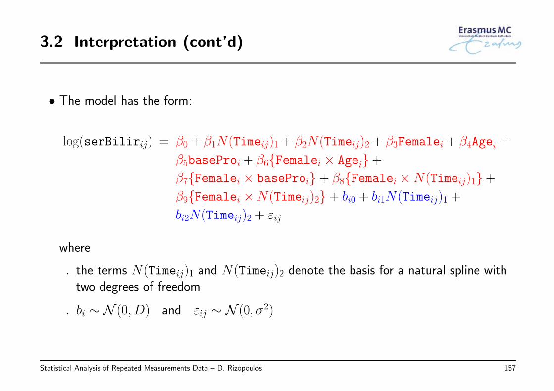
3.2 Interpretation (cont’d)
• The model has the form:
log(serBilirij) = β0 + β1N(Timeij)1 + β2N(Timeij)2 + β3Femalei + β4Agei +
β5baseProi + β6{Femalei × Agei} +β7{Femalei × baseProi} + β8{Femalei ×N(Timeij)1} +β9{Femalei ×N(Timeij)2} + bi0 + bi1N(Timeij)1 +
bi2N(Timeij)2 + εij
where
◃ the terms N(Timeij)1 and N(Timeij)2 denote the basis for a natural spline withtwo degrees of freedom
◃ bi ∼ N (0, D) and εij ∼ N (0, σ2)
Statistical Analysis of Repeated Measurements Data – D. Rizopoulos 157
3.2 Interpretation (cont’d)
• In this model not all coefficients have a direct interpretation in isolation
• Hence to understand the model we depict
◃ how the average longitudinal profiles evolve over time,
◃ separately for males and females, and prothrombin time of 10.6 sec
◃ for the average age of 49 years old
◃ including also the corresponding 95% pointwise confidence intervals
◃ (in the app different ages and prothrombin times can be selected)
Statistical Analysis of Repeated Measurements Data – D. Rizopoulos 158
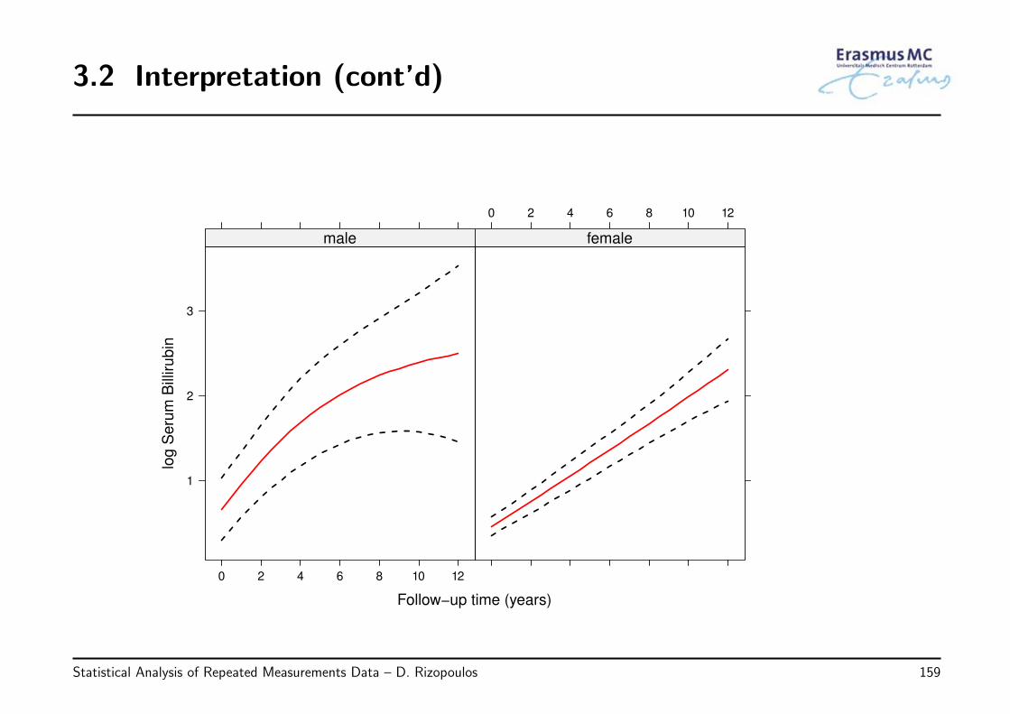
3.2 Interpretation (cont’d)
Follow−up time (years)
log
Se
rum
Bill
iru
bin
1
2
3
0 2 4 6 8 10 12
male
0 2 4 6 8 10 12
female
Statistical Analysis of Repeated Measurements Data – D. Rizopoulos 159
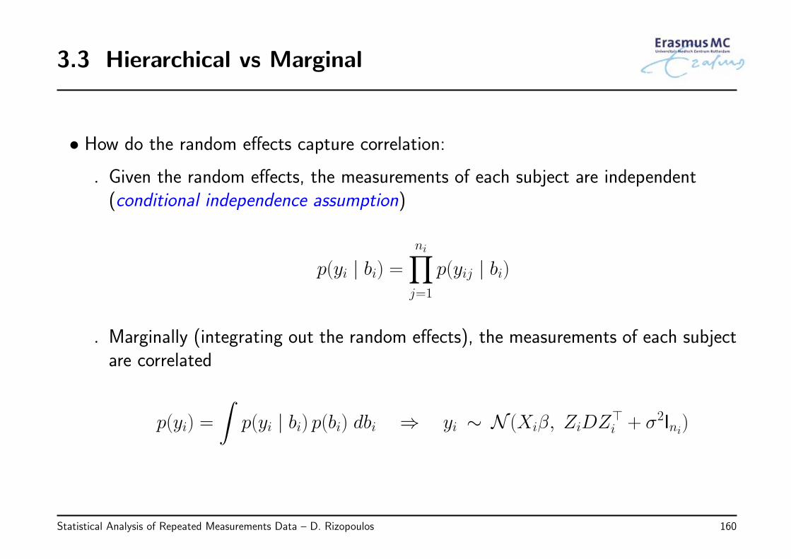
3.3 Hierarchical vs Marginal
• How do the random effects capture correlation:
◃ Given the random effects, the measurements of each subject are independent(conditional independence assumption)
p(yi | bi) =ni∏j=1
p(yij | bi)
◃ Marginally (integrating out the random effects), the measurements of each subjectare correlated
p(yi) =
∫p(yi | bi) p(bi) dbi ⇒ yi ∼ N (Xiβ, ZiDZ⊤
i + σ2Ini)
Statistical Analysis of Repeated Measurements Data – D. Rizopoulos 160
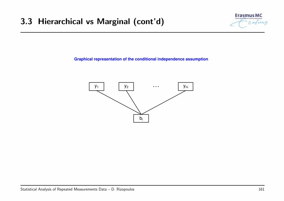
3.3 Hierarchical vs Marginal (cont’d)
Graphical representation of the conditional independence assumption
y1 y2 yni
bi
…
Statistical Analysis of Repeated Measurements Data – D. Rizopoulos 161
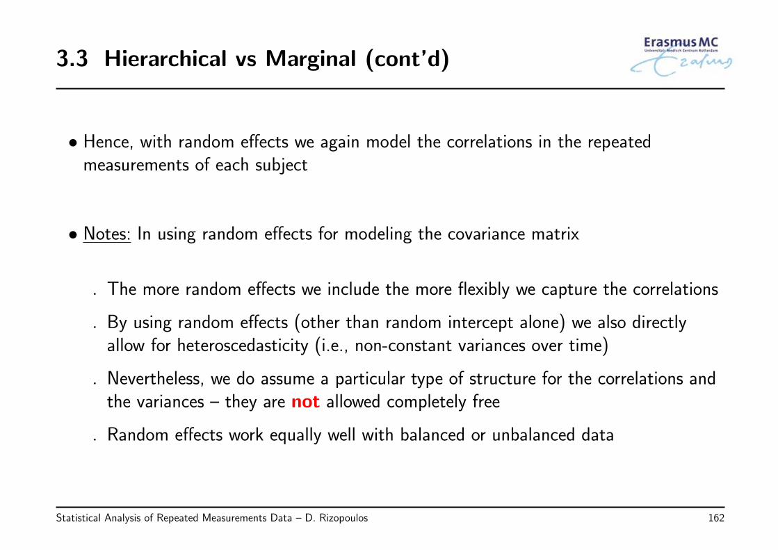
3.3 Hierarchical vs Marginal (cont’d)
• Hence, with random effects we again model the correlations in the repeatedmeasurements of each subject
• Notes: In using random effects for modeling the covariance matrix
◃ The more random effects we include the more flexibly we capture the correlations
◃ By using random effects (other than random intercept alone) we also directlyallow for heteroscedasticity (i.e., non-constant variances over time)
◃ Nevertheless, we do assume a particular type of structure for the correlations andthe variances – they are not allowed completely free
◃ Random effects work equally well with balanced or unbalanced data
Statistical Analysis of Repeated Measurements Data – D. Rizopoulos 162
3.3 Hierarchical vs Marginal (cont’d)
• Let’s try the app. . .
Statistical Analysis of Repeated Measurements Data – D. Rizopoulos 163
3.3 Hierarchical vs Marginal (cont’d)
• Hierarchical formulation
◃ a model for yi given bi, and a model for bi
◃ D is the covariance matrix of the random effects ⇒ needs to be positivedefinite
• Marginal formulation
◃ a model for yi, and a specific form of the marginal covariance matrixVi = ZiDZ⊤
i + σ2Ini
◃ only Vi needs to be positive definite
◃ Vi can be positive definite without D being positive definite
Statistical Analysis of Repeated Measurements Data – D. Rizopoulos 164
3.3 Hierarchical vs Marginal (cont’d)
The hierarchical model implies the marginal one,not vice versa
• A simple example: Random-intercepts modelyij = β0 + β1tij + bi0 + εij,
bi0 ∼ N (0, σ2b ), εij ∼ N (0, σ2).
Statistical Analysis of Repeated Measurements Data – D. Rizopoulos 165
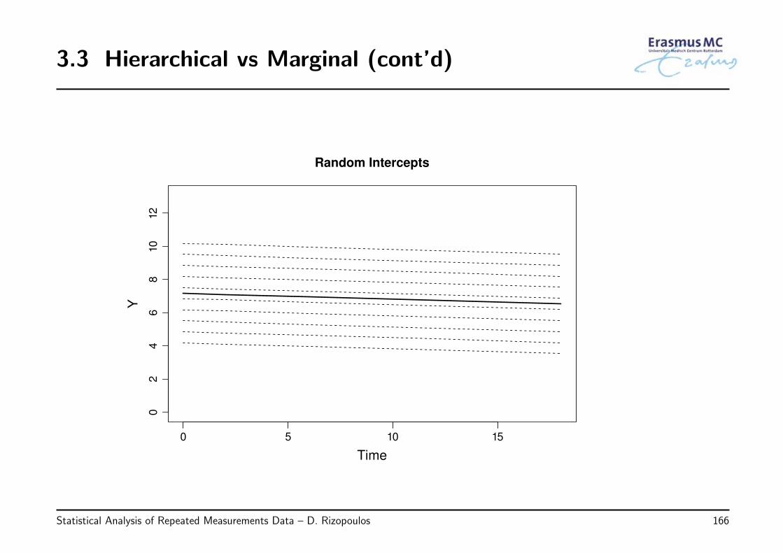
3.3 Hierarchical vs Marginal (cont’d)
0 5 10 15
02
46
810
12
Random Intercepts
Time
Y
Statistical Analysis of Repeated Measurements Data – D. Rizopoulos 166
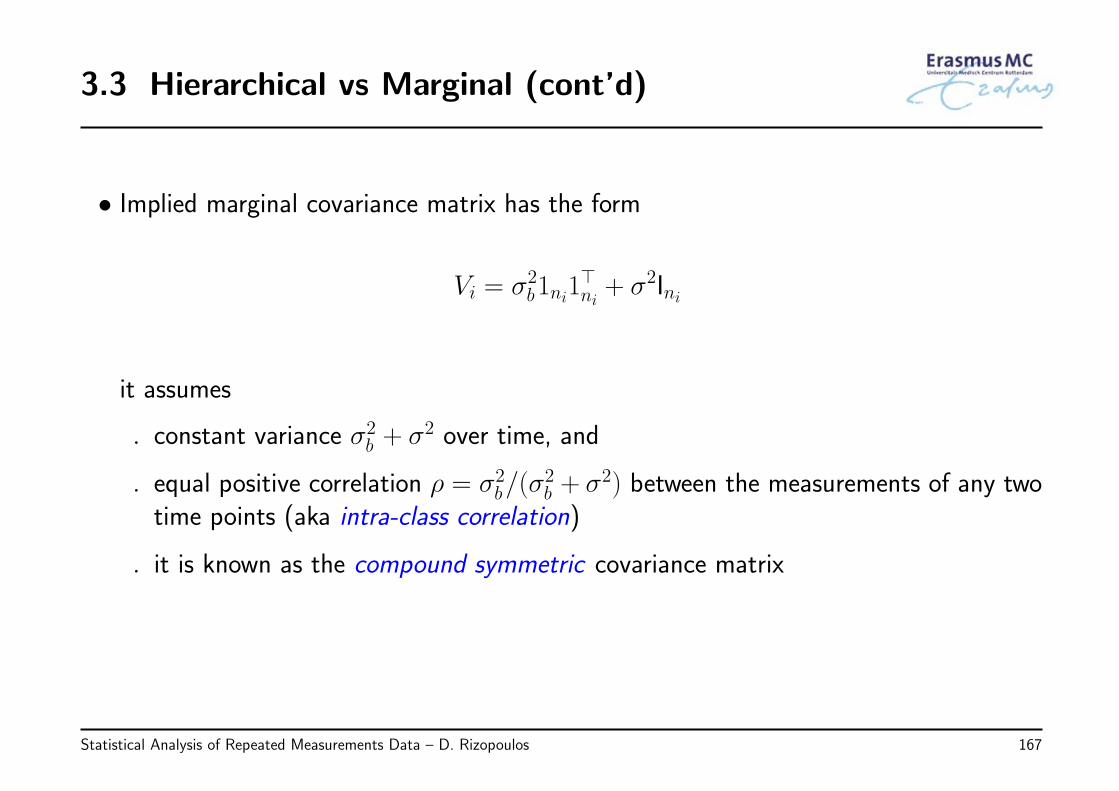
3.3 Hierarchical vs Marginal (cont’d)
• Implied marginal covariance matrix has the form
Vi = σ2b1ni1
⊤ni+ σ2Ini
it assumes
◃ constant variance σ2b + σ2 over time, and
◃ equal positive correlation ρ = σ2b/(σ
2b + σ2) between the measurements of any two
time points (aka intra-class correlation)
◃ it is known as the compound symmetric covariance matrix
Statistical Analysis of Repeated Measurements Data – D. Rizopoulos 167
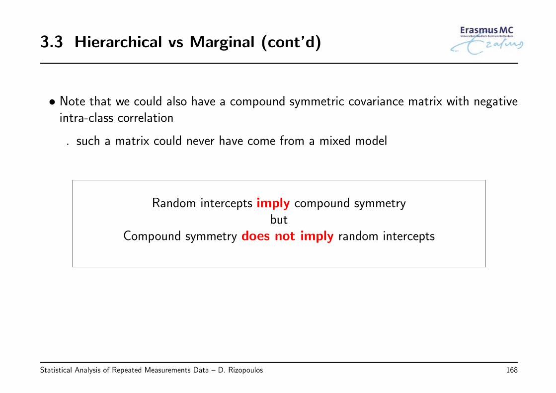
3.3 Hierarchical vs Marginal (cont’d)
• Note that we could also have a compound symmetric covariance matrix with negativeintra-class correlation
◃ such a matrix could never have come from a mixed model
Random intercepts imply compound symmetrybut
Compound symmetry does not imply random intercepts
Statistical Analysis of Repeated Measurements Data – D. Rizopoulos 168
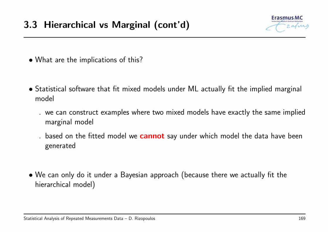
3.3 Hierarchical vs Marginal (cont’d)
• What are the implications of this?
• Statistical software that fit mixed models under ML actually fit the implied marginalmodel
◃ we can construct examples where two mixed models have exactly the same impliedmarginal model
◃ based on the fitted model we cannot say under which model the data have beengenerated
• We can only do it under a Bayesian approach (because there we actually fit thehierarchical model)
Statistical Analysis of Repeated Measurements Data – D. Rizopoulos 169
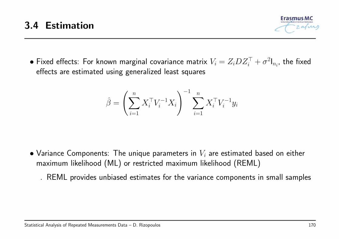
3.4 Estimation
• Fixed effects: For known marginal covariance matrix Vi = ZiDZ⊤i + σ2Ini, the fixed
effects are estimated using generalized least squares
β =
(n∑
i=1
X⊤i V
−1i Xi
)−1 n∑i=1
X⊤i V
−1i yi
• Variance Components: The unique parameters in Vi are estimated based on eithermaximum likelihood (ML) or restricted maximum likelihood (REML)
◃ REML provides unbiased estimates for the variance components in small samples
Statistical Analysis of Repeated Measurements Data – D. Rizopoulos 170
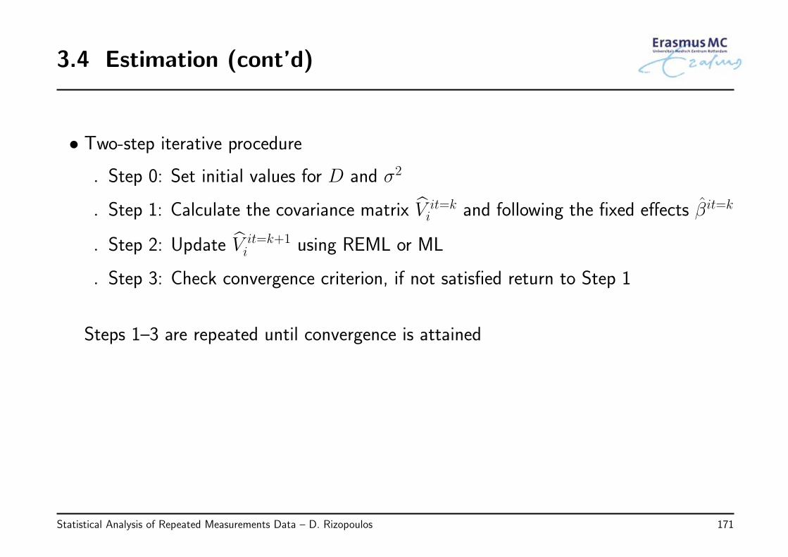
3.4 Estimation (cont’d)
• Two-step iterative procedure
◃ Step 0: Set initial values for D and σ2
◃ Step 1: Calculate the covariance matrix V it=ki and following the fixed effects βit=k
◃ Step 2: Update V it=k+1i using REML or ML
◃ Step 3: Check convergence criterion, if not satisfied return to Step 1
Steps 1–3 are repeated until convergence is attained
Statistical Analysis of Repeated Measurements Data – D. Rizopoulos 171
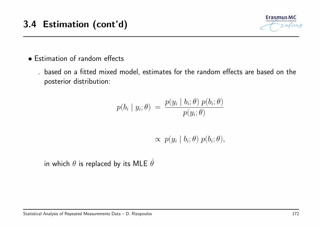
3.4 Estimation (cont’d)
• Estimation of random effects
◃ based on a fitted mixed model, estimates for the random effects are based on theposterior distribution:
p(bi | yi; θ) =p(yi | bi; θ) p(bi; θ)
p(yi; θ)
∝ p(yi | bi; θ) p(bi; θ),
in which θ is replaced by its MLE θ
Statistical Analysis of Repeated Measurements Data – D. Rizopoulos 172
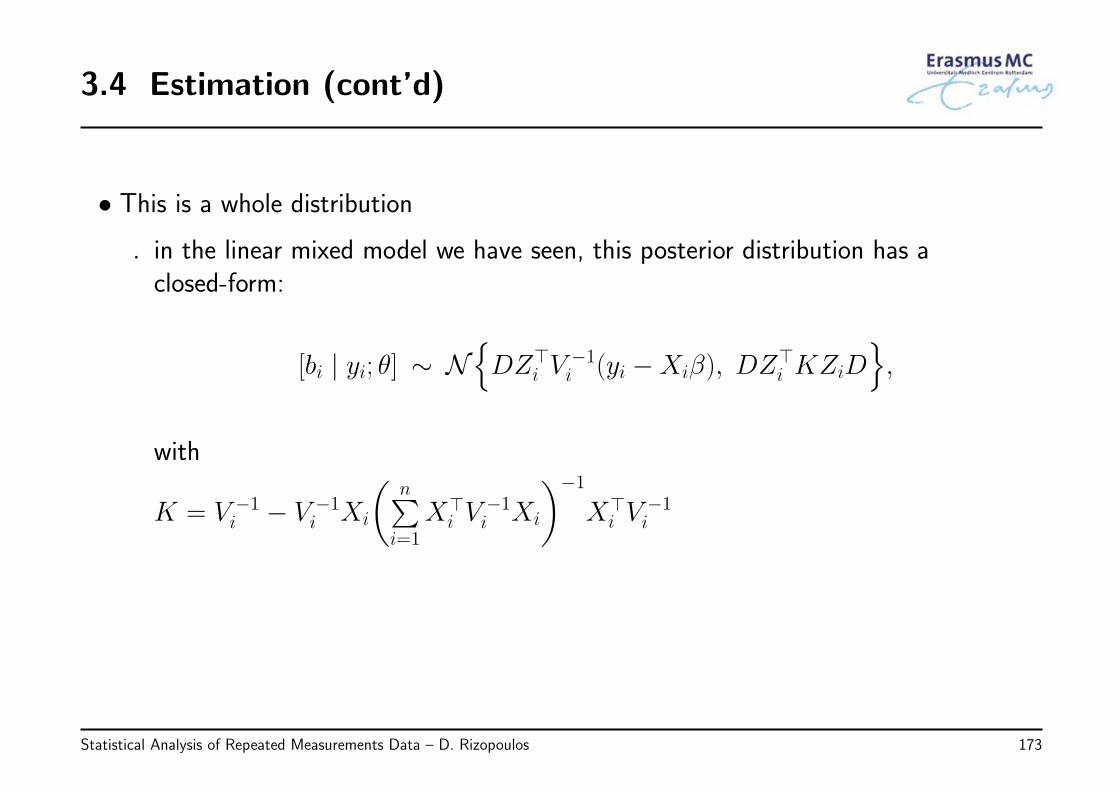
3.4 Estimation (cont’d)
• This is a whole distribution
◃ in the linear mixed model we have seen, this posterior distribution has aclosed-form:
[bi | yi; θ] ∼ N{DZ⊤
i V−1i (yi −Xiβ), DZ⊤
i KZiD},
with
K = V −1i − V −1
i Xi
(n∑i=1
X⊤i V
−1i Xi
)−1
X⊤i V
−1i
Statistical Analysis of Repeated Measurements Data – D. Rizopoulos 173
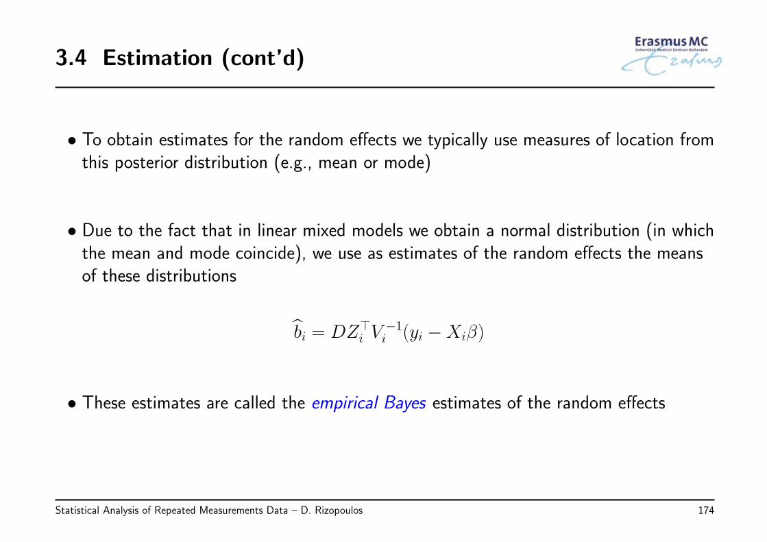
3.4 Estimation (cont’d)
• To obtain estimates for the random effects we typically use measures of location fromthis posterior distribution (e.g., mean or mode)
• Due to the fact that in linear mixed models we obtain a normal distribution (in whichthe mean and mode coincide), we use as estimates of the random effects the meansof these distributions
bi = DZ⊤i V
−1i (yi −Xiβ)
• These estimates are called the empirical Bayes estimates of the random effects
Statistical Analysis of Repeated Measurements Data – D. Rizopoulos 174
3.4 Estimation (cont’d)
• Estimates of the random effects are very useful in prediction
◃ in this context there is an important difference between the marginal models wehave seen in Chapter 2 and the mixed models of this chapter
• In particular, the predictions from a marginal model are
ymargi = Xiβ
whereas from the mixed model we obtain
ysubji = Xiβ + Zibi
Statistical Analysis of Repeated Measurements Data – D. Rizopoulos 175
3.4 Estimation (cont’d)
• The difference is that
◃ from the marginal model we obtain predictions for the ‘average’ patient havingcharacteristics Xi (i.e., age, sex, etc.)
◃ from the mixed model we obtain predictions for the ‘average’ patient that hascharacteristics Xi and observed data yi (i.e., they have a subject-specific nature)
• The predictions Xiβ + Zibi we obtain from the mixed model are called the BestLinear Unbiased Predictions (BLUPs)
◃ ‘linear’ because they are a linear combination of β and bi
◃ ‘unbiased’ because their average equals the true subject-specific mean
◃ ‘best’ because they have the smallest variance of all linear predictors
Statistical Analysis of Repeated Measurements Data – D. Rizopoulos 176
3.4 Estimation (cont’d)
• Example: To see an example of the difference between the marginal andsubject-specific predictions, we compare the two sets of predictions for the complexlinear mixed model we have seen in Section 3.2 (pp.156–159) for 16 randomlyselected patients
◃ red lines denote the marginal predictions,
◃ blue lines denote the subject-specific predictions
◃ black circles the observed data
Statistical Analysis of Repeated Measurements Data – D. Rizopoulos 177
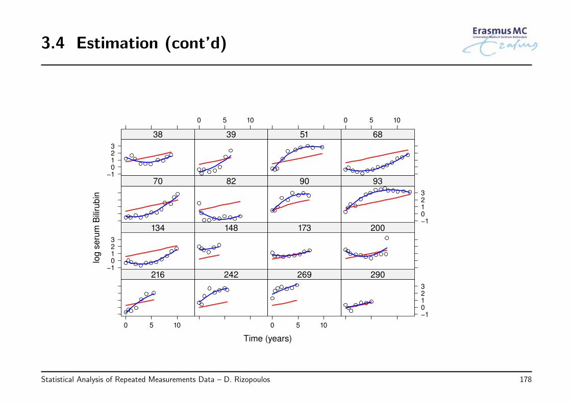
3.4 Estimation (cont’d)
Time (years)
log
se
rum
Bili
rub
in
−10123
38
0 5 10
39 51
0 5 10
68
70 82 90
−10123
93
−10123
134 148 173 200
0 5 10
216 242
0 5 10
269
−10123
290
Statistical Analysis of Repeated Measurements Data – D. Rizopoulos 178
3.4 Estimation (cont’d)
• We clearly observe that the subject-specific predictions are much closer to the data ofeach individual patient than the marginal ones
Statistical Analysis of Repeated Measurements Data – D. Rizopoulos 179
3.5 Mixed-Effects Models in R
R> There are two primary packages in R for mixed models analysis:
◃ Package nlme
* fits linear & nonlinear mixed effects models, and marginal models for normaldata
* allows for both random effects & correlated error terms
* several options for covariances matrices and variance functions
◃ Package lme4
* fits linear, nonlinear & generalized mixed effects models
* uses only random effects
* allows for nested and crossed random-effects designs
Statistical Analysis of Repeated Measurements Data – D. Rizopoulos 180
3.5 Mixed-Effects Models in R (cont’d)
R> The basic function to fit linear mixed models in the nlme package is lme(), andhas three basic arguments
◃ fixed: a formula specifying the response vector and the fixed-effects structure
◃ random: a formula specifying the random-effects structure
◃ data: a data frame containing all the variables
Statistical Analysis of Repeated Measurements Data – D. Rizopoulos 181

3.5 Mixed-Effects Models in R (cont’d)
R> The data frame that contains all variables should be in the long format
Subject y time gender age
1 5.1 0.0 male 45
1 6.3 1.1 male 45
2 5.9 0.1 female 38
2 6.9 0.9 female 38
2 7.1 1.2 female 38
2 7.3 1.5 female 38... ... ... ... ...
Statistical Analysis of Repeated Measurements Data – D. Rizopoulos 182
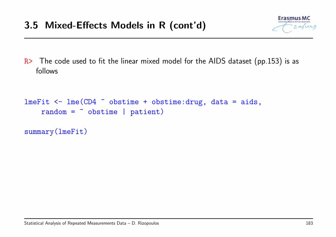
3.5 Mixed-Effects Models in R (cont’d)
R> The code used to fit the linear mixed model for the AIDS dataset (pp.153) is asfollows
lmeFit <- lme(CD4 ~ obstime + obstime:drug, data = aids,
random = ~ obstime | patient)
summary(lmeFit)
Statistical Analysis of Repeated Measurements Data – D. Rizopoulos 183
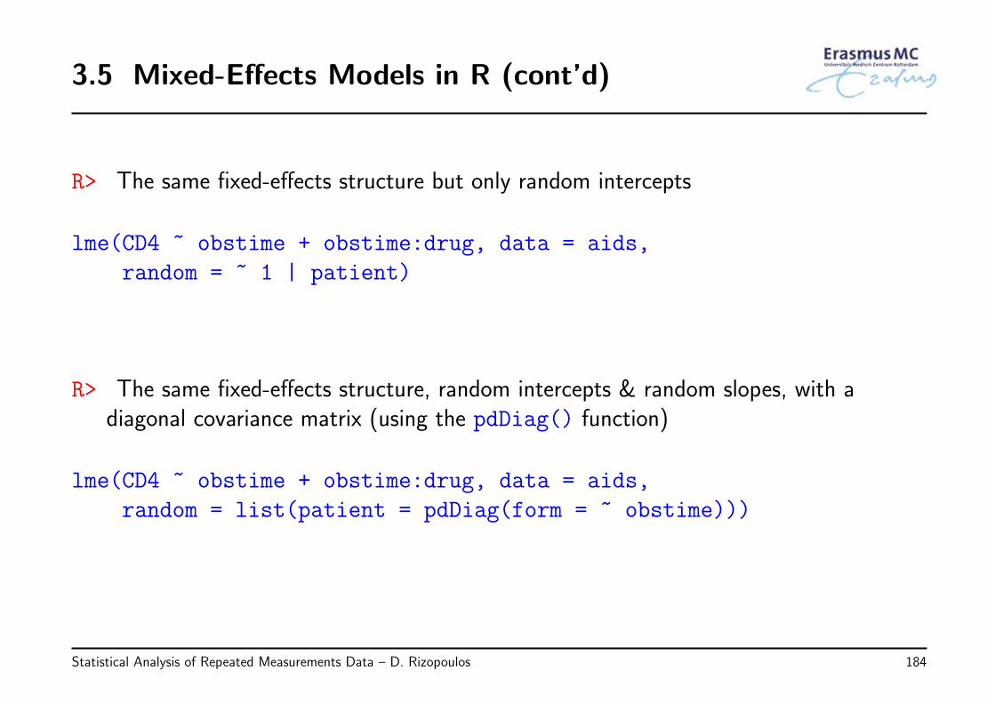
3.5 Mixed-Effects Models in R (cont’d)
R> The same fixed-effects structure but only random intercepts
lme(CD4 ~ obstime + obstime:drug, data = aids,
random = ~ 1 | patient)
R> The same fixed-effects structure, random intercepts & random slopes, with adiagonal covariance matrix (using the pdDiag() function)
lme(CD4 ~ obstime + obstime:drug, data = aids,
random = list(patient = pdDiag(form = ~ obstime)))
Statistical Analysis of Repeated Measurements Data – D. Rizopoulos 184
3.5 Mixed-Effects Models in R (cont’d)
R> The basic function to fit linear mixed models in the lme4 package is lmer(), andhas two basic arguments
◃ formula: a formula specifying the response vector, the fixed- and random-effectsstructure
◃ data: a data frame containing all the variables
R> Again the data should be in the long format
Statistical Analysis of Repeated Measurements Data – D. Rizopoulos 185
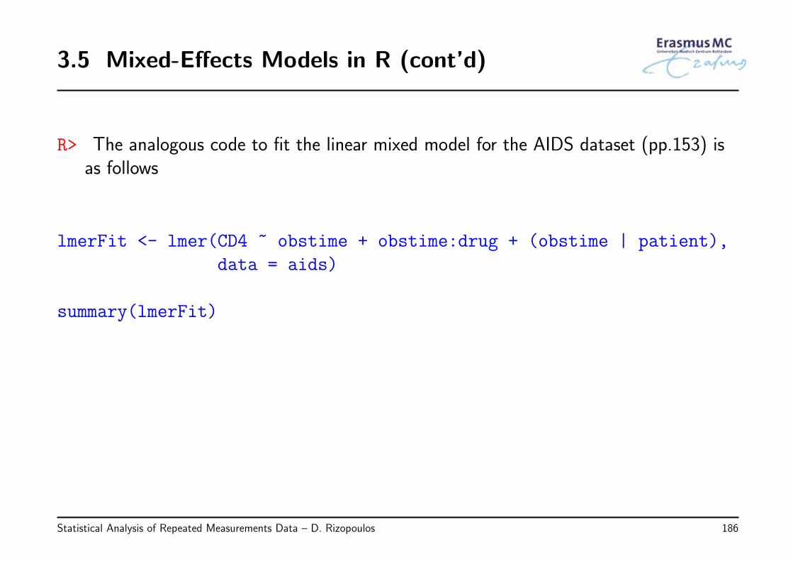
3.5 Mixed-Effects Models in R (cont’d)
R> The analogous code to fit the linear mixed model for the AIDS dataset (pp.153) isas follows
lmerFit <- lmer(CD4 ~ obstime + obstime:drug + (obstime | patient),
data = aids)
summary(lmerFit)
Statistical Analysis of Repeated Measurements Data – D. Rizopoulos 186
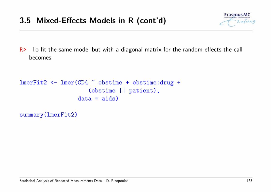
3.5 Mixed-Effects Models in R (cont’d)
R> To fit the same model but with a diagonal matrix for the random effects the callbecomes:
lmerFit2 <- lmer(CD4 ~ obstime + obstime:drug +
(obstime || patient),
data = aids)
summary(lmerFit2)
Statistical Analysis of Repeated Measurements Data – D. Rizopoulos 187
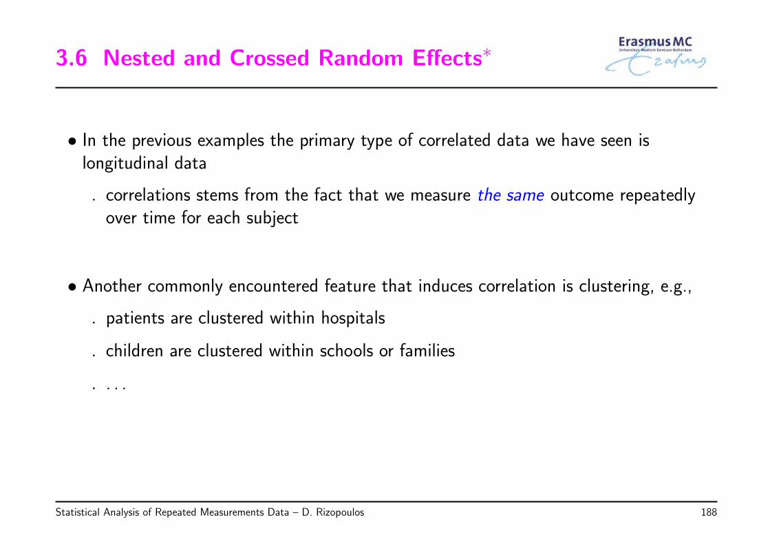
3.6 Nested and Crossed Random Effects∗
• In the previous examples the primary type of correlated data we have seen islongitudinal data
◃ correlations stems from the fact that we measure the same outcome repeatedlyover time for each subject
• Another commonly encountered feature that induces correlation is clustering, e.g.,
◃ patients are clustered within hospitals
◃ children are clustered within schools or families
◃ . . .
Statistical Analysis of Repeated Measurements Data – D. Rizopoulos 188
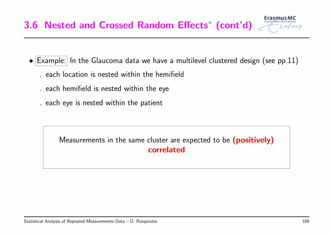
3.6 Nested and Crossed Random Effects∗ (cont’d)
• Example: In the Glaucoma data we have a multilevel clustered design (see pp.11)
◃ each location is nested within the hemifield
◃ each hemifield is nested within the eye
◃ each eye is nested within the patient
Measurements in the same cluster are expected to be (positively)correlated
Statistical Analysis of Repeated Measurements Data – D. Rizopoulos 189
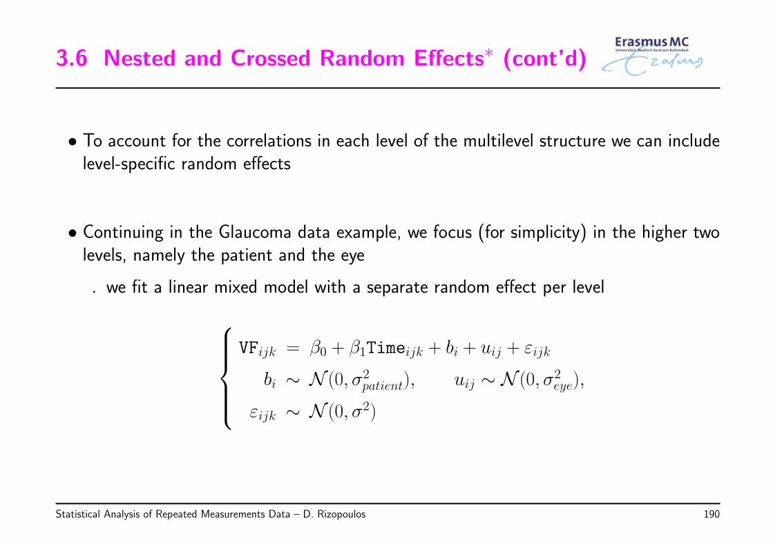
3.6 Nested and Crossed Random Effects∗ (cont’d)
• To account for the correlations in each level of the multilevel structure we can includelevel-specific random effects
• Continuing in the Glaucoma data example, we focus (for simplicity) in the higher twolevels, namely the patient and the eye
◃ we fit a linear mixed model with a separate random effect per levelVFijk = β0 + β1Timeijk + bi + uij + εijk
bi ∼ N (0, σ2patient), uij ∼ N (0, σ2
eye),
εijk ∼ N (0, σ2)
Statistical Analysis of Repeated Measurements Data – D. Rizopoulos 190
3.6 Nested and Crossed Random Effects∗ (cont’d)
where
◃ VFijk denotes the k-th visual field sensitivity measurement for the j-th eye of thei-th patient
◃ Timeijk denotes the corresponding time point this measurement was taken
◃ bi is the random effect for the patients – the measurements of the i-th patient arecorrelated because all these measurements share the same random effect bi
◃ uij is the random effect for the eye within the patient – the measurements of thej-th eye of the i-th patient are more correlated than the measurements of thej′-th eye because they share the same random effect uij
Statistical Analysis of Repeated Measurements Data – D. Rizopoulos 191
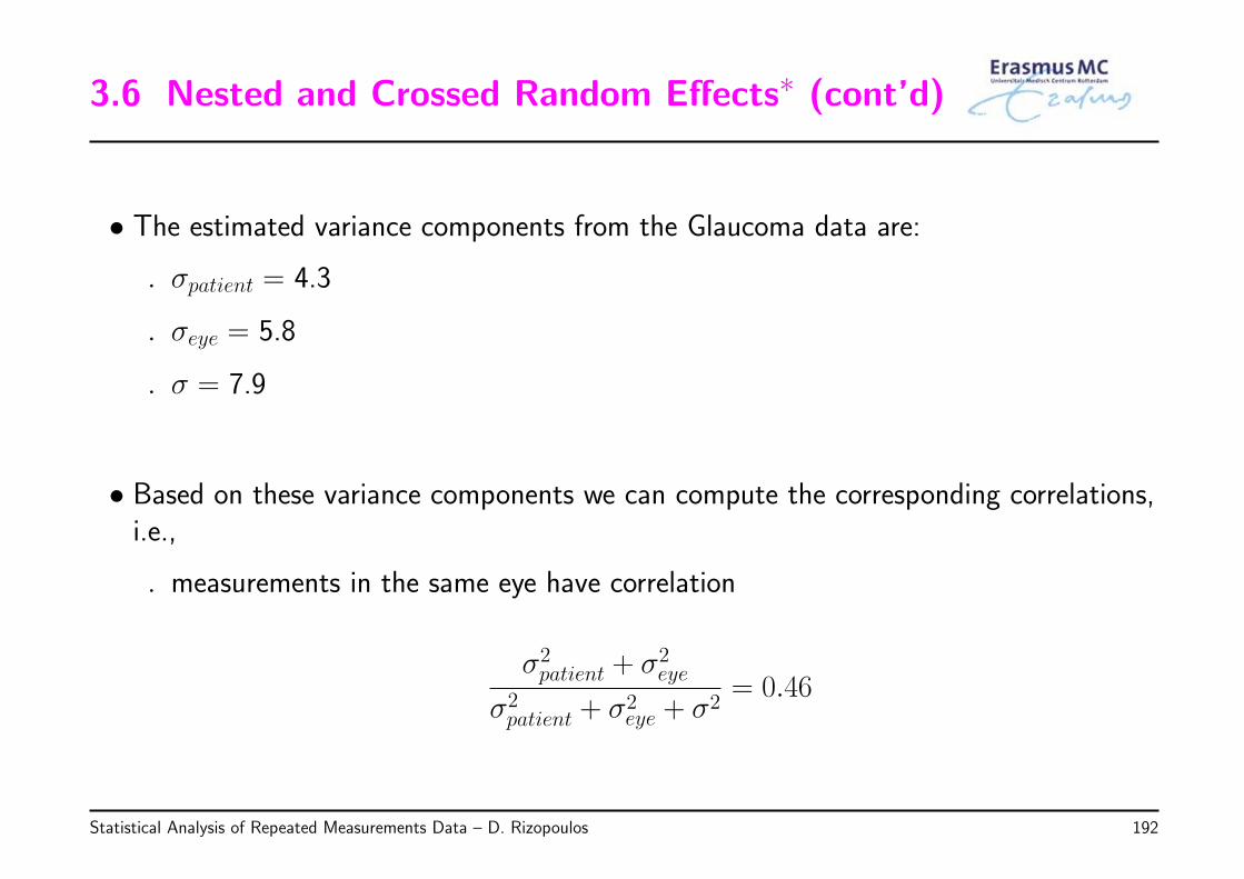
3.6 Nested and Crossed Random Effects∗ (cont’d)
• The estimated variance components from the Glaucoma data are:
◃ σpatient = 4.3
◃ σeye = 5.8
◃ σ = 7.9
• Based on these variance components we can compute the corresponding correlations,i.e.,
◃ measurements in the same eye have correlation
σ2patient + σ2
eye
σ2patient + σ2
eye + σ2= 0.46
Statistical Analysis of Repeated Measurements Data – D. Rizopoulos 192
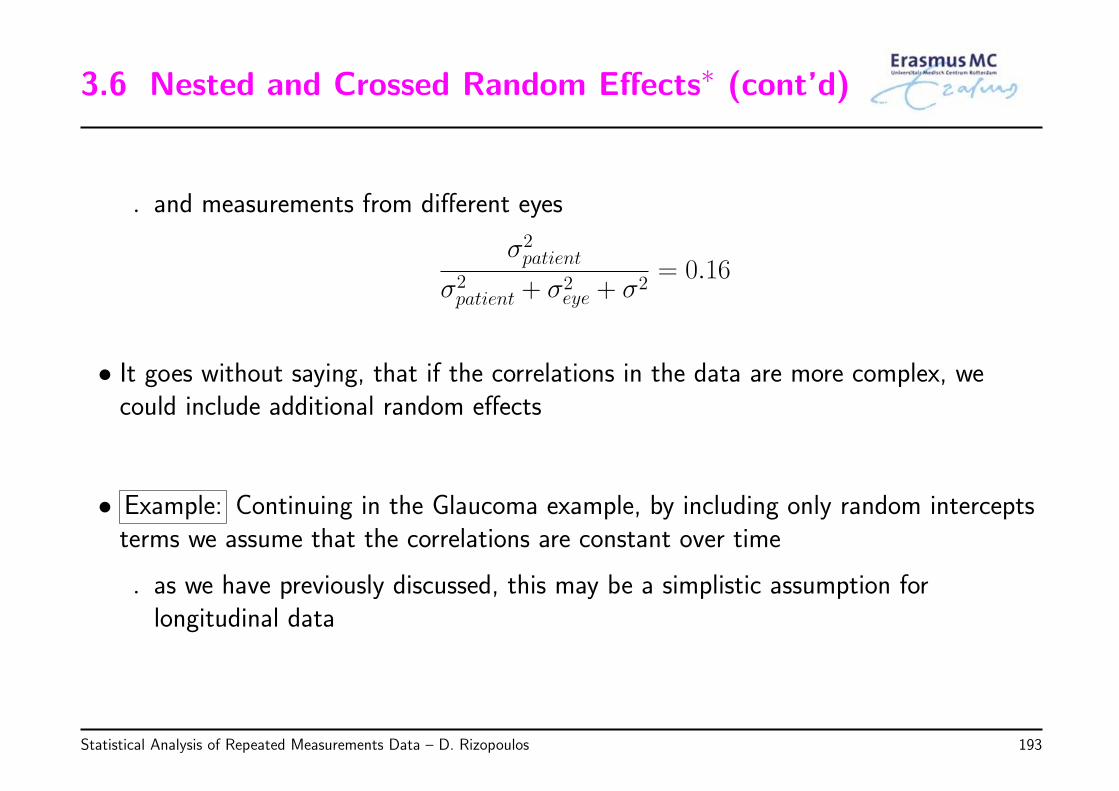
3.6 Nested and Crossed Random Effects∗ (cont’d)
◃ and measurements from different eyes
σ2patient
σ2patient + σ2
eye + σ2= 0.16
• It goes without saying, that if the correlations in the data are more complex, wecould include additional random effects
• Example: Continuing in the Glaucoma example, by including only random interceptsterms we assume that the correlations are constant over time
◃ as we have previously discussed, this may be a simplistic assumption forlongitudinal data
Statistical Analysis of Repeated Measurements Data – D. Rizopoulos 193
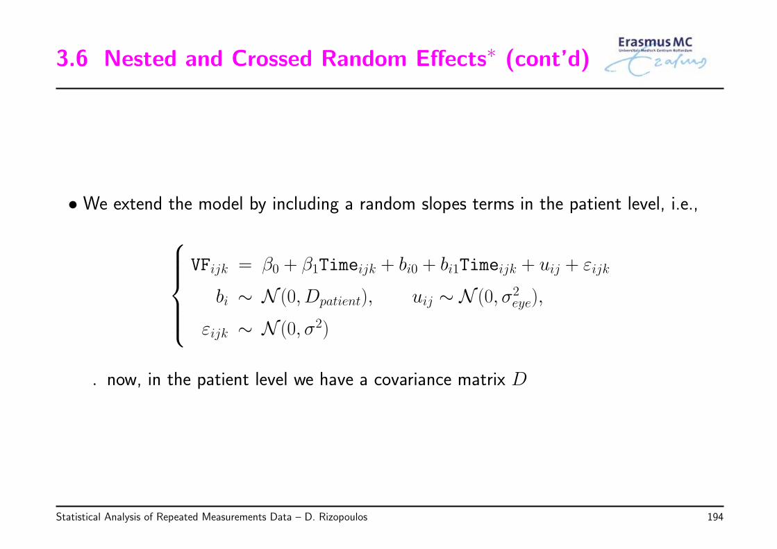
3.6 Nested and Crossed Random Effects∗ (cont’d)
• We extend the model by including a random slopes terms in the patient level, i.e.,VFijk = β0 + β1Timeijk + bi0 + bi1Timeijk + uij + εijk
bi ∼ N (0, Dpatient), uij ∼ N (0, σ2eye),
εijk ∼ N (0, σ2)
◃ now, in the patient level we have a covariance matrix D
Statistical Analysis of Repeated Measurements Data – D. Rizopoulos 194
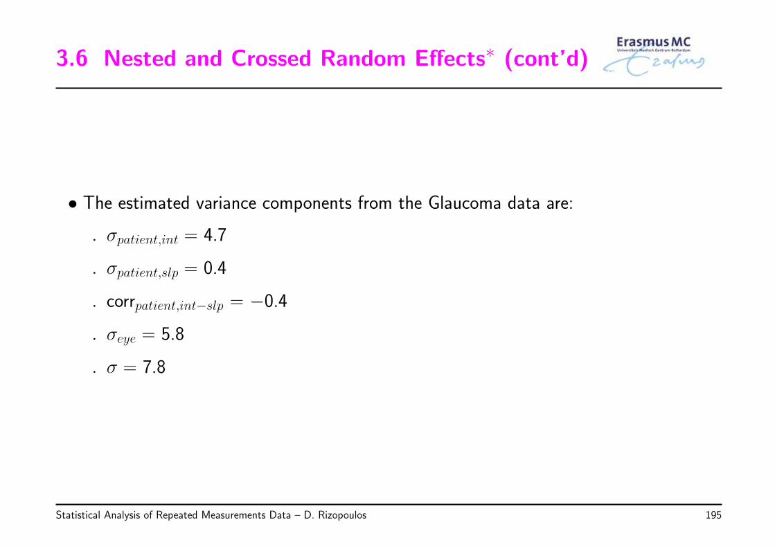
3.6 Nested and Crossed Random Effects∗ (cont’d)
• The estimated variance components from the Glaucoma data are:
◃ σpatient,int = 4.7
◃ σpatient,slp = 0.4
◃ corrpatient,int−slp = −0.4
◃ σeye = 5.8
◃ σ = 7.8
Statistical Analysis of Repeated Measurements Data – D. Rizopoulos 195
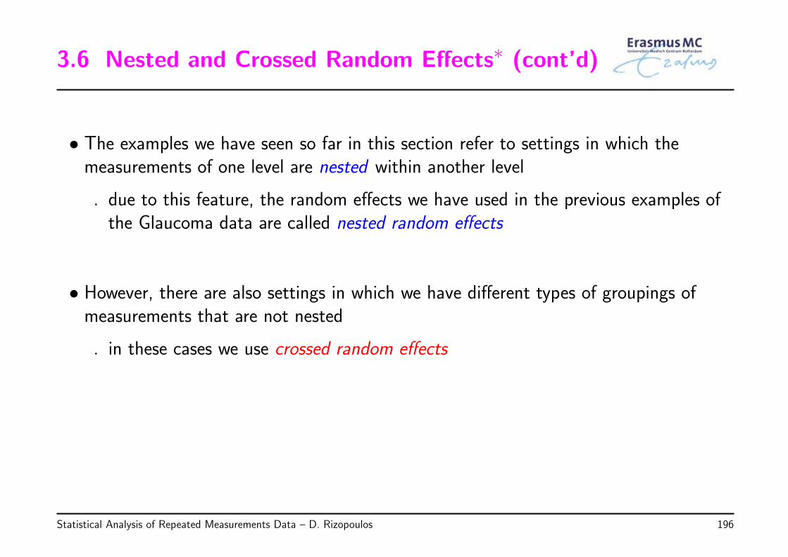
3.6 Nested and Crossed Random Effects∗ (cont’d)
• The examples we have seen so far in this section refer to settings in which themeasurements of one level are nested within another level
◃ due to this feature, the random effects we have used in the previous examples ofthe Glaucoma data are called nested random effects
• However, there are also settings in which we have different types of groupings ofmeasurements that are not nested
◃ in these cases we use crossed random effects
Statistical Analysis of Repeated Measurements Data – D. Rizopoulos 196
3.6 Nested and Crossed Random Effects∗ (cont’d)
• Example: One feature of visual field sensitivity measurements is that they exhibit theso-called Global Visit Effect (see pp.12)
◃ in particular, for some visits some patients showed strangely low sensitivity to thestimuli
◃ in the next visit, their sensitivity levels improved
◃ it is not possible this low sensitivity to be due to Glaucoma because it is anirreparable disease
◃ hence, the low sensitivity measurements are attributed to other reasons (e.g.,tiredness)
• To capture this Global Visit Effect we can include a random effect for each visit
◃ this random effect is not nested to the previously used random effects
Statistical Analysis of Repeated Measurements Data – D. Rizopoulos 197
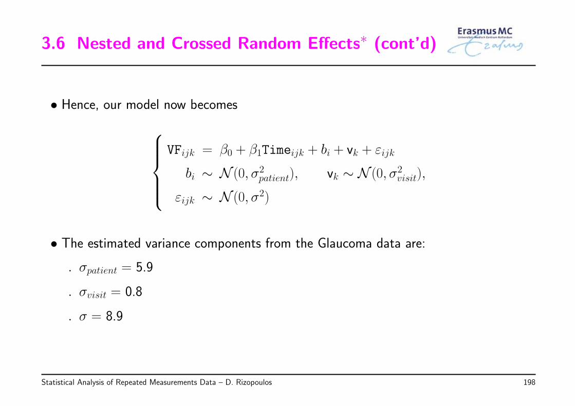
3.6 Nested and Crossed Random Effects∗ (cont’d)
• Hence, our model now becomesVFijk = β0 + β1Timeijk + bi + vk + εijk
bi ∼ N (0, σ2patient), vk ∼ N (0, σ2
visit),
εijk ∼ N (0, σ2)
• The estimated variance components from the Glaucoma data are:
◃ σpatient = 5.9
◃ σvisit = 0.8
◃ σ = 8.9
Statistical Analysis of Repeated Measurements Data – D. Rizopoulos 198
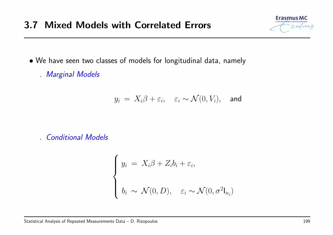
3.7 Mixed Models with Correlated Errors
• We have seen two classes of models for longitudinal data, namely
◃ Marginal Models
yi = Xiβ + εi, εi ∼ N (0, Vi), and
◃ Conditional Models yi = Xiβ + Zibi + εi,
bi ∼ N (0, D), εi ∼ N (0, σ2Ini)
Statistical Analysis of Repeated Measurements Data – D. Rizopoulos 199
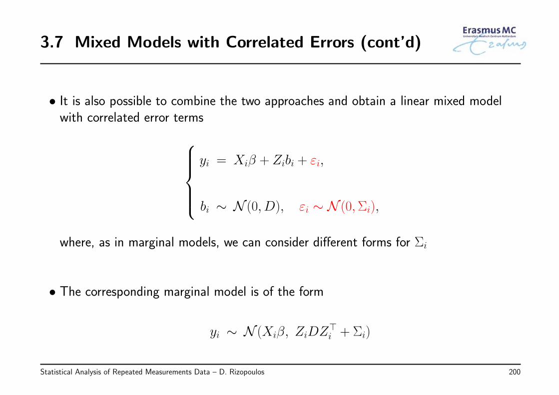
3.7 Mixed Models with Correlated Errors (cont’d)
• It is also possible to combine the two approaches and obtain a linear mixed modelwith correlated error terms
yi = Xiβ + Zibi + εi,
bi ∼ N (0, D), εi ∼ N (0,Σi),
where, as in marginal models, we can consider different forms for Σi
• The corresponding marginal model is of the form
yi ∼ N (Xiβ, ZiDZ⊤i + Σi)
Statistical Analysis of Repeated Measurements Data – D. Rizopoulos 200
3.7 Mixed Models with Correlated Errors (cont’d)
• Features
◃ both bi and Σi try to capture the correlation in the observed responses yi
◃ this model does not assume conditional independence
• Choice between the two approaches is to a large extent philosophical
◃ Random Effects: trajectory of a subject dictated by time-independent randomeffects ⇒ the shape of the trajectory is an inherent characteristic of this subject
◃ Serial Correlation: attempts to more precisely capture features of the trajectory byallowing subject-specific trends to vary over time
Statistical Analysis of Repeated Measurements Data – D. Rizopoulos 201
3.7 Mixed Models with Correlated Errors (cont’d)
Often in practice it is not possible to include both a serial correlation term andmany random effects because of numerical problems
• Example: In the AIDS dataset we investigate the fit of a mixed model withexponential serial correlation and increasing number of random effects – in particular:
◃ Model I: random intercepts
◃ Model II: random intercepts & random slopes
the fixed-effects part includes linear and quadratic slopes and their interaction withtreatment
Statistical Analysis of Repeated Measurements Data – D. Rizopoulos 202
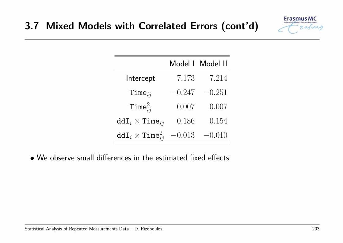
3.7 Mixed Models with Correlated Errors (cont’d)
Model I Model II
Intercept 7.173 7.214
Timeij −0.247 −0.251
Time2ij 0.007 0.007
ddIi × Timeij 0.186 0.154
ddIi × Time2ij −0.013 −0.010
• We observe small differences in the estimated fixed effects
Statistical Analysis of Repeated Measurements Data – D. Rizopoulos 203
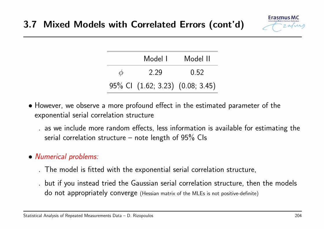
3.7 Mixed Models with Correlated Errors (cont’d)
Model I Model II
ϕ 2.29 0.52
95% CI (1.62; 3.23) (0.08; 3.45)
• However, we observe a more profound effect in the estimated parameter of theexponential serial correlation structure
◃ as we include more random effects, less information is available for estimating theserial correlation structure – note length of 95% CIs
• Numerical problems:
◃ The model is fitted with the exponential serial correlation structure,
◃ but if you instead tried the Gaussian serial correlation structure, then the modelsdo not appropriately converge (Hessian matrix of the MLEs is not positive-definite)
Statistical Analysis of Repeated Measurements Data – D. Rizopoulos 204
3.8 Time-Varying Covariates∗
• Up to now we have only included in mixed models covariates, which were fixed frombaseline (except of course the time variable)
• However, often we may also be interested in assessing how a longitudinal outcome isassociated with a covariate whose value changes over time
◃ such covariates are called time-varying covariates
• Example: In the PBC dataset we are interested in the effect of prothrombin time onserum bilirubin – prothrombin time has also been collected longitudinally duringfollow-up
Statistical Analysis of Repeated Measurements Data – D. Rizopoulos 205
3.8 Time-Varying Covariates∗ (cont’d)
• The handling of time-varying covariates poses some important challenges:
1. Not always the longitudinal outcome and the time-varying covariate are collectedat the same time points
2. The longitudinal outcome at a particular time point t may depend not only on thevalue of the covariate at the same time point but also at other time points
3. There are two types of time-varying covariates, endogenous and exogenous
◃ a time-varying covariate is exogenous if its distribution at time t is conditionallyindependent of all preceding outcomes
◃ a time-varying covariate is endogenous if it is not exogenous
Statistical Analysis of Repeated Measurements Data – D. Rizopoulos 206
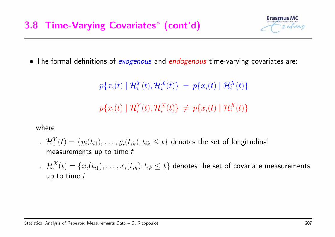
3.8 Time-Varying Covariates∗ (cont’d)
• The formal definitions of exogenous and endogenous time-varying covariates are:
p{xi(t) | HYi (t),HX
i (t)} = p{xi(t) | HXi (t)}
p{xi(t) | HYi (t),HX
i (t)} = p{xi(t) | HXi (t)}
where
◃ HYi (t) = {yi(ti1), . . . , yi(tik); tik ≤ t} denotes the set of longitudinal
measurements up to time t
◃ HXi (t) = {xi(ti1), . . . , xi(tik); tik ≤ t} denotes the set of covariate measurements
up to time t
Statistical Analysis of Repeated Measurements Data – D. Rizopoulos 207
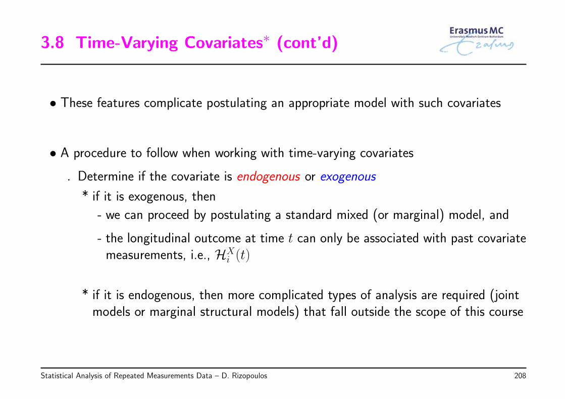
3.8 Time-Varying Covariates∗ (cont’d)
• These features complicate postulating an appropriate model with such covariates
• A procedure to follow when working with time-varying covariates
◃ Determine if the covariate is endogenous or exogenous
* if it is exogenous, then
- we can proceed by postulating a standard mixed (or marginal) model, and
- the longitudinal outcome at time t can only be associated with past covariatemeasurements, i.e., HX
i (t)
* if it is endogenous, then more complicated types of analysis are required (jointmodels or marginal structural models) that fall outside the scope of this course
Statistical Analysis of Repeated Measurements Data – D. Rizopoulos 208
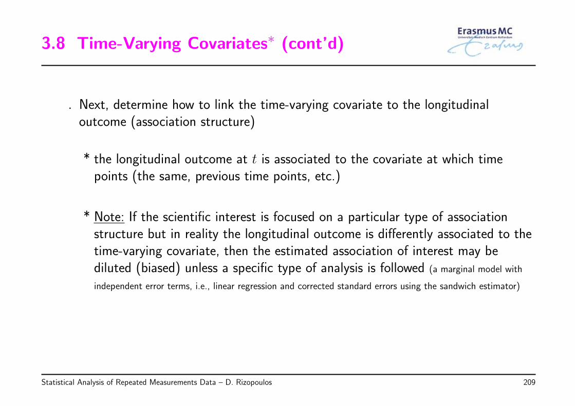
3.8 Time-Varying Covariates∗ (cont’d)
◃ Next, determine how to link the time-varying covariate to the longitudinaloutcome (association structure)
* the longitudinal outcome at t is associated to the covariate at which timepoints (the same, previous time points, etc.)
* Note: If the scientific interest is focused on a particular type of associationstructure but in reality the longitudinal outcome is differently associated to thetime-varying covariate, then the estimated association of interest may bediluted (biased) unless a specific type of analysis is followed (a marginal model with
independent error terms, i.e., linear regression and corrected standard errors using the sandwich estimator)
Statistical Analysis of Repeated Measurements Data – D. Rizopoulos 209
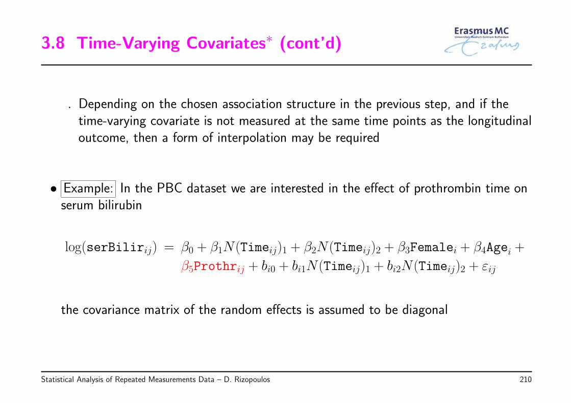
3.8 Time-Varying Covariates∗ (cont’d)
◃ Depending on the chosen association structure in the previous step, and if thetime-varying covariate is not measured at the same time points as the longitudinaloutcome, then a form of interpolation may be required
• Example: In the PBC dataset we are interested in the effect of prothrombin time onserum bilirubin
log(serBilirij) = β0 + β1N(Timeij)1 + β2N(Timeij)2 + β3Femalei + β4Agei +
β5Prothrij + bi0 + bi1N(Timeij)1 + bi2N(Timeij)2 + εij
the covariance matrix of the random effects is assumed to be diagonal
Statistical Analysis of Repeated Measurements Data – D. Rizopoulos 210
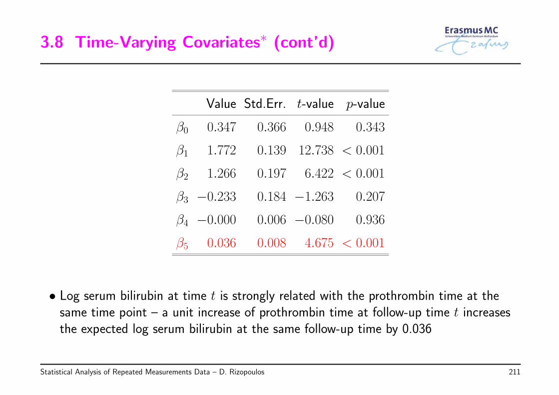
3.8 Time-Varying Covariates∗ (cont’d)
Value Std.Err. t-value p-value
β0 0.347 0.366 0.948 0.343
β1 1.772 0.139 12.738 < 0.001
β2 1.266 0.197 6.422 < 0.001
β3 −0.233 0.184 −1.263 0.207
β4 −0.000 0.006 −0.080 0.936
β5 0.036 0.008 4.675 < 0.001
• Log serum bilirubin at time t is strongly related with the prothrombin time at thesame time point – a unit increase of prothrombin time at follow-up time t increasesthe expected log serum bilirubin at the same follow-up time by 0.036
Statistical Analysis of Repeated Measurements Data – D. Rizopoulos 211
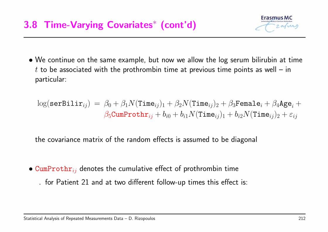
3.8 Time-Varying Covariates∗ (cont’d)
• We continue on the same example, but now we allow the log serum bilirubin at timet to be associated with the prothrombin time at previous time points as well – inparticular:
log(serBilirij) = β0 + β1N(Timeij)1 + β2N(Timeij)2 + β3Femalei + β4Agei +
β5CumProthrij + bi0 + bi1N(Timeij)1 + bi2N(Timeij)2 + εij
the covariance matrix of the random effects is assumed to be diagonal
• CumProthrij denotes the cumulative effect of prothrombin time
◃ for Patient 21 and at two different follow-up times this effect is:
Statistical Analysis of Repeated Measurements Data – D. Rizopoulos 212
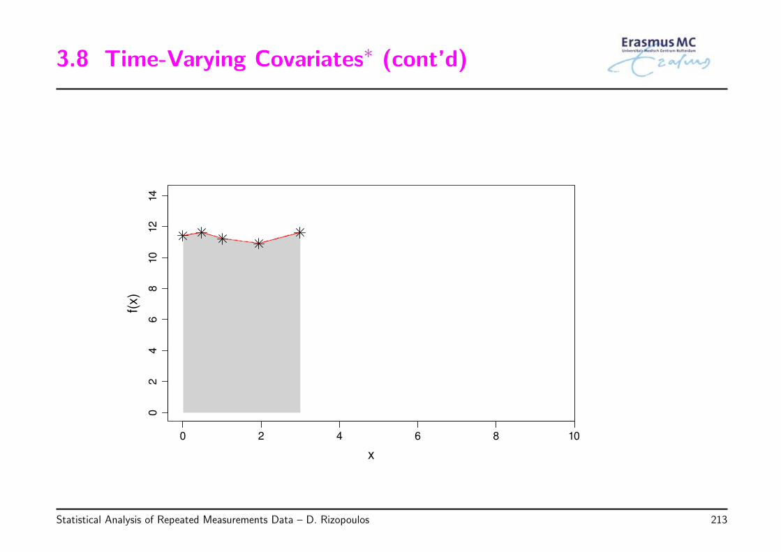
3.8 Time-Varying Covariates∗ (cont’d)
0 2 4 6 8 10
02
46
810
12
14
x
f(x)
Statistical Analysis of Repeated Measurements Data – D. Rizopoulos 213
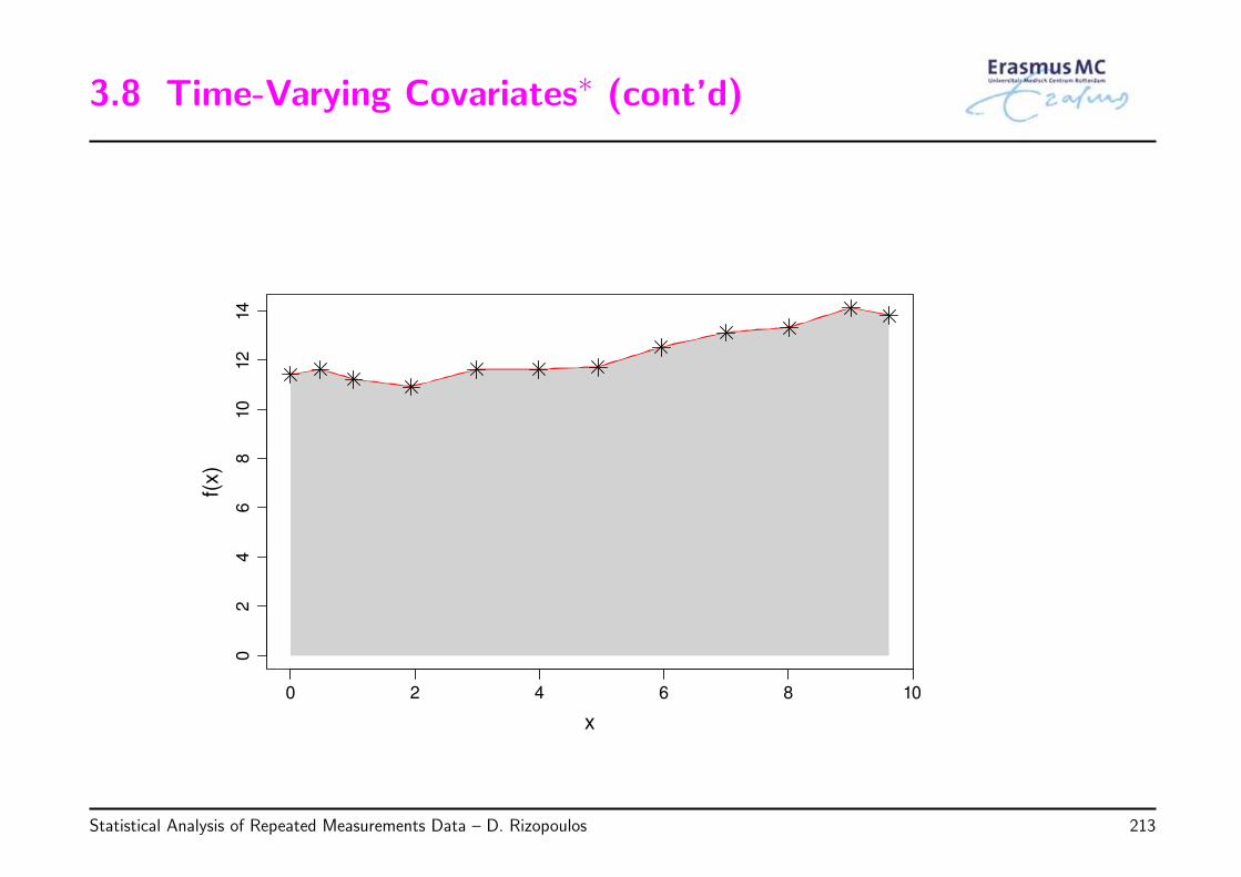
3.8 Time-Varying Covariates∗ (cont’d)
0 2 4 6 8 10
02
46
810
12
14
x
f(x)
Statistical Analysis of Repeated Measurements Data – D. Rizopoulos 213
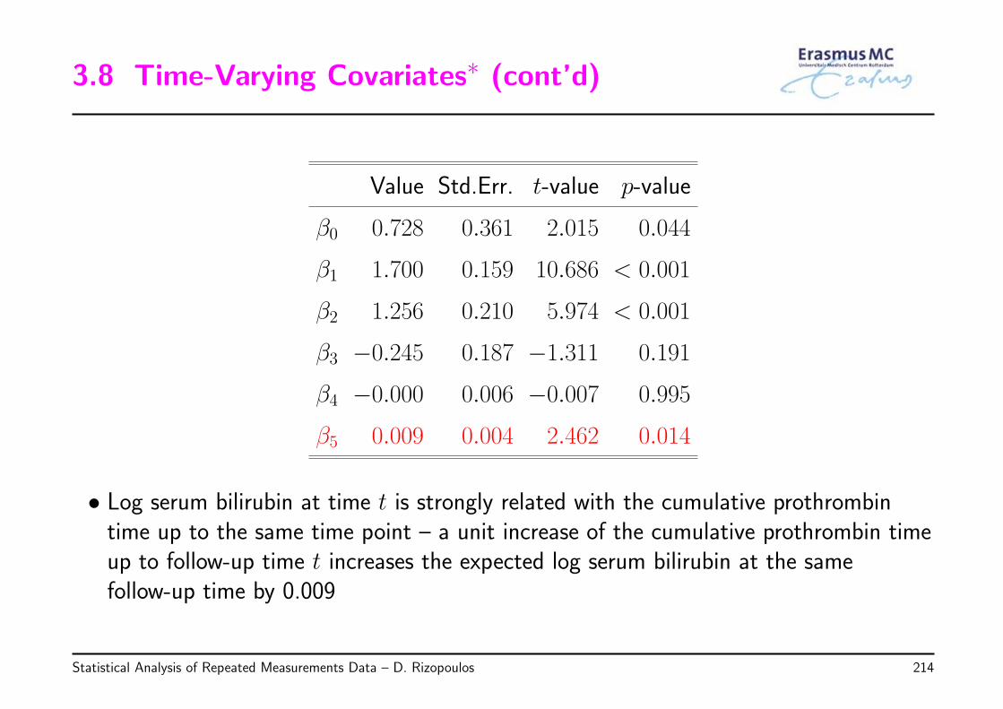
3.8 Time-Varying Covariates∗ (cont’d)
Value Std.Err. t-value p-value
β0 0.728 0.361 2.015 0.044
β1 1.700 0.159 10.686 < 0.001
β2 1.256 0.210 5.974 < 0.001
β3 −0.245 0.187 −1.311 0.191
β4 −0.000 0.006 −0.007 0.995
β5 0.009 0.004 2.462 0.014
• Log serum bilirubin at time t is strongly related with the cumulative prothrombintime up to the same time point – a unit increase of the cumulative prothrombin timeup to follow-up time t increases the expected log serum bilirubin at the samefollow-up time by 0.009
Statistical Analysis of Repeated Measurements Data – D. Rizopoulos 214
3.9 Model Building
• Mixed models consist of two parts, namely
◃ fixed effects that describe how specific covariates influence the averagelongitudinal evolutions
◃ random effects that describe how specific regression coefficients deviate from theoverall mean described by the fixed effects
* the random effects also model the correlations in the repeated measurements
• Interest can either be
◃ on the fixed-effects part alone (e.g., does treatment influence the averageevolutions) or
◃ on both parts (e.g., to obtain subject specific predictions)
Statistical Analysis of Repeated Measurements Data – D. Rizopoulos 215
3.9 Model Building (cont’d)
• The general model building strategy we have seen in the previous chapter formarginal models also applies in the case of mixed models – more specifically:
1. Put all the covariates of interest in the fixed-effects part, considering possiblenonlinear terms and/or interactions between them – do NOT remove the onesthat are not significant
2. Then select an appropriate random-effects structure that adequately describes thecorrelations in the repeated measurements
* typically we start from random intercepts and include each time an additionalrandom effect term to see if we improve the fit (i.e., random slopes, quadraticrandom slopes, etc.)
* you should be a bit anti-conservative, i.e., do not favor a simpler covariancematrix if the p-value is just non-significant
Statistical Analysis of Repeated Measurements Data – D. Rizopoulos 216
3.9 Model Building (cont’d)
3. Finally, return to the mean part and exclude non significant covariates
* first start by testing the nonlinear & interaction terms
Statistical Analysis of Repeated Measurements Data – D. Rizopoulos 217
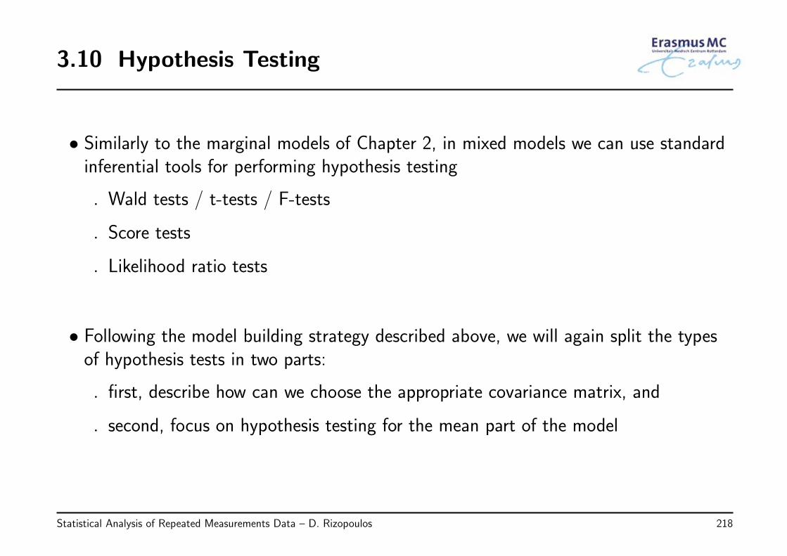
3.10 Hypothesis Testing
• Similarly to the marginal models of Chapter 2, in mixed models we can use standardinferential tools for performing hypothesis testing
◃ Wald tests / t-tests / F-tests
◃ Score tests
◃ Likelihood ratio tests
• Following the model building strategy described above, we will again split the typesof hypothesis tests in two parts:
◃ first, describe how can we choose the appropriate covariance matrix, and
◃ second, focus on hypothesis testing for the mean part of the model
Statistical Analysis of Repeated Measurements Data – D. Rizopoulos 218
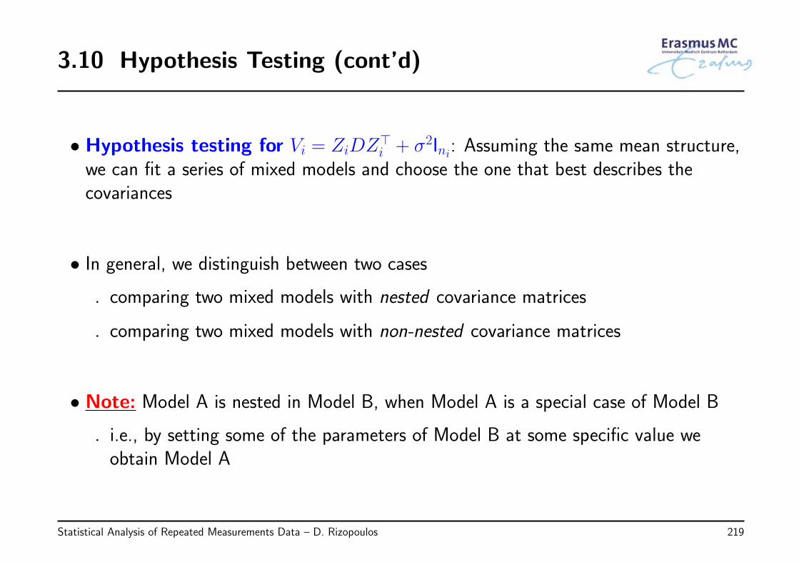
3.10 Hypothesis Testing (cont’d)
• Hypothesis testing for Vi = ZiDZ⊤i + σ2Ini: Assuming the same mean structure,
we can fit a series of mixed models and choose the one that best describes thecovariances
• In general, we distinguish between two cases
◃ comparing two mixed models with nested covariance matrices
◃ comparing two mixed models with non-nested covariance matrices
• Note: Model A is nested in Model B, when Model A is a special case of Model B
◃ i.e., by setting some of the parameters of Model B at some specific value weobtain Model A
Statistical Analysis of Repeated Measurements Data – D. Rizopoulos 219

3.10 Hypothesis Testing (cont’d)
• For nested models the preferable test for selecting Vi is the likelihood ratio test(LRT):
LRT = −2× {ℓ(θ0)− ℓ(θa)} ∼ χ2p
where
◃ ℓ(θ0) the value of the log-likelihood function under the null hypothesis, i.e., thespecial case model
◃ ℓ(θa) the value of the log-likelihood function under the alternative hypothesis, i.e.,the general model
◃ p denotes the number of parameters being tested
• Note: Provided that the mean structure in the two models is the same, we caneither compare the REML of ML likelihoods of the models (preferable is REML)
Statistical Analysis of Repeated Measurements Data – D. Rizopoulos 220
3.10 Hypothesis Testing (cont’d)
Though, there is a technical complication when we compare nestedmixed models for which one model has more random effects than the
other
Statistical Analysis of Repeated Measurements Data – D. Rizopoulos 221
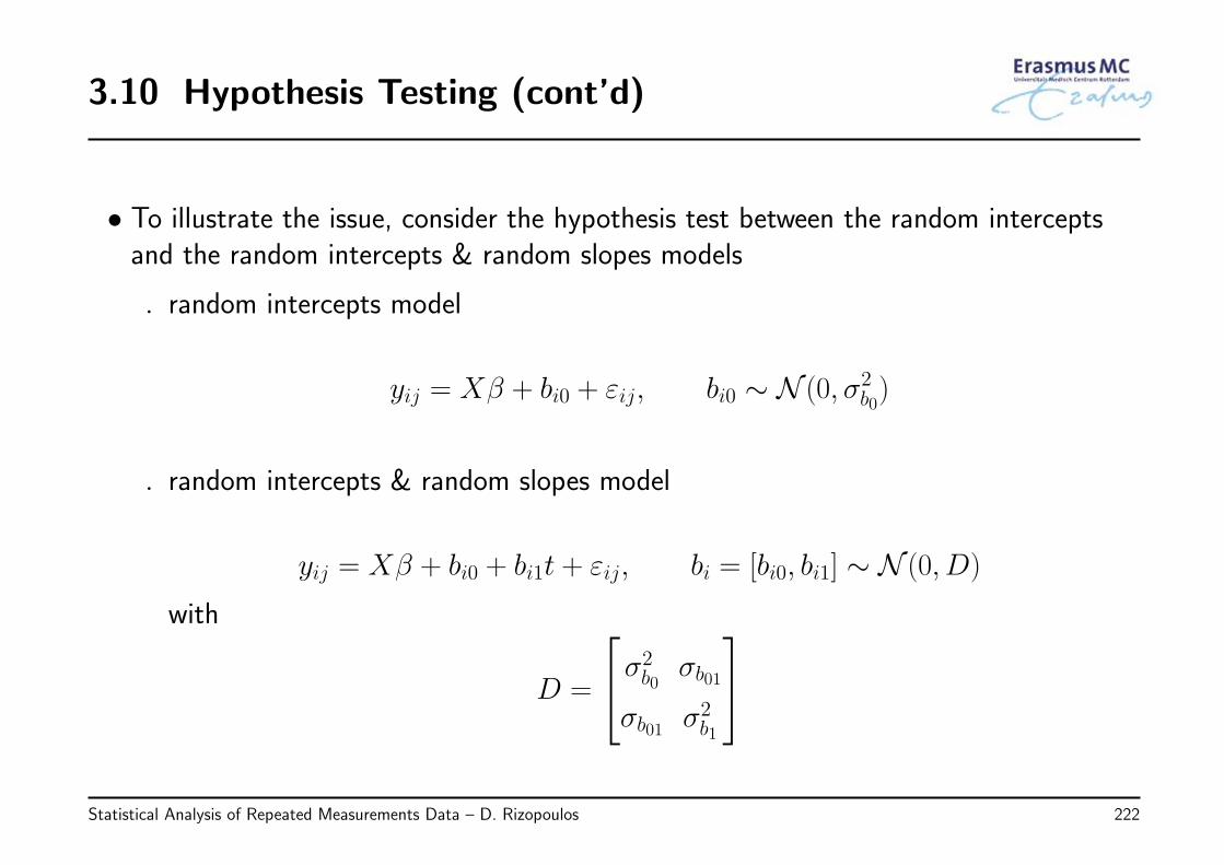
3.10 Hypothesis Testing (cont’d)
• To illustrate the issue, consider the hypothesis test between the random interceptsand the random intercepts & random slopes models
◃ random intercepts model
yij = Xβ + bi0 + εij, bi0 ∼ N (0, σ2b0)
◃ random intercepts & random slopes model
yij = Xβ + bi0 + bi1t + εij, bi = [bi0, bi1] ∼ N (0, D)
with
D =
σ2b0
σb01
σb01 σ2b1
Statistical Analysis of Repeated Measurements Data – D. Rizopoulos 222
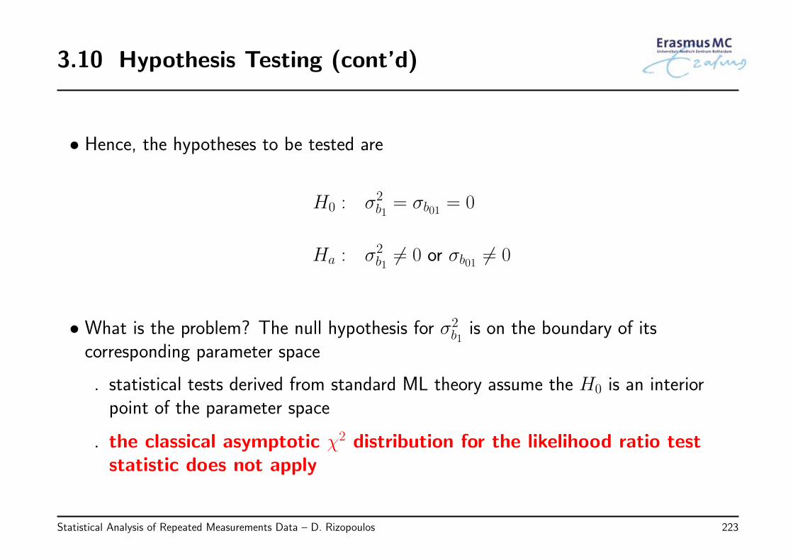
3.10 Hypothesis Testing (cont’d)
• Hence, the hypotheses to be tested are
H0 : σ2b1= σb01 = 0
Ha : σ2b1= 0 or σb01 = 0
• What is the problem? The null hypothesis for σ2b1is on the boundary of its
corresponding parameter space
◃ statistical tests derived from standard ML theory assume the H0 is an interiorpoint of the parameter space
◃ the classical asymptotic χ2 distribution for the likelihood ratio teststatistic does not apply
Statistical Analysis of Repeated Measurements Data – D. Rizopoulos 223
3.10 Hypothesis Testing (cont’d)
• For simple settings (as the one above), it has been proposed to use a mixture of χ2
distributions to derive p-values, namely
◃ 50% from the χ2 distribution with degrees of freedom the number of parametersbeing tested, and
◃ 50% from the χ2 distribution with degrees of freedom the number of parameterswhich are not on the boundary under H0
• Nonetheless, it has been suggested that this solution does not always worksatisfactorily
◃ e.g., see package RLRsim in R and the references therein
Statistical Analysis of Repeated Measurements Data – D. Rizopoulos 224
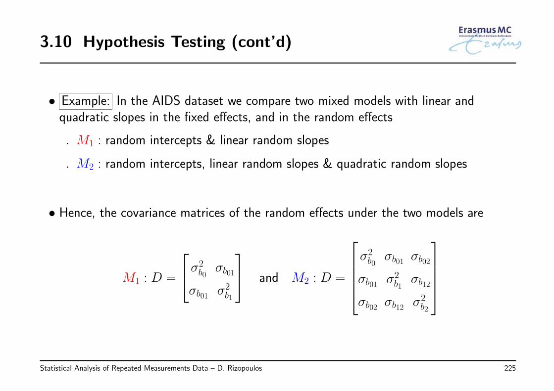
3.10 Hypothesis Testing (cont’d)
• Example: In the AIDS dataset we compare two mixed models with linear andquadratic slopes in the fixed effects, and in the random effects
◃ M1 : random intercepts & linear random slopes
◃ M2 : random intercepts, linear random slopes & quadratic random slopes
• Hence, the covariance matrices of the random effects under the two models are
M1 : D =
σ2b0
σb01
σb01 σ2b1
and M2 : D =
σ2b0
σb01 σb02
σb01 σ2b1
σb12
σb02 σb12 σ2b2
Statistical Analysis of Repeated Measurements Data – D. Rizopoulos 225
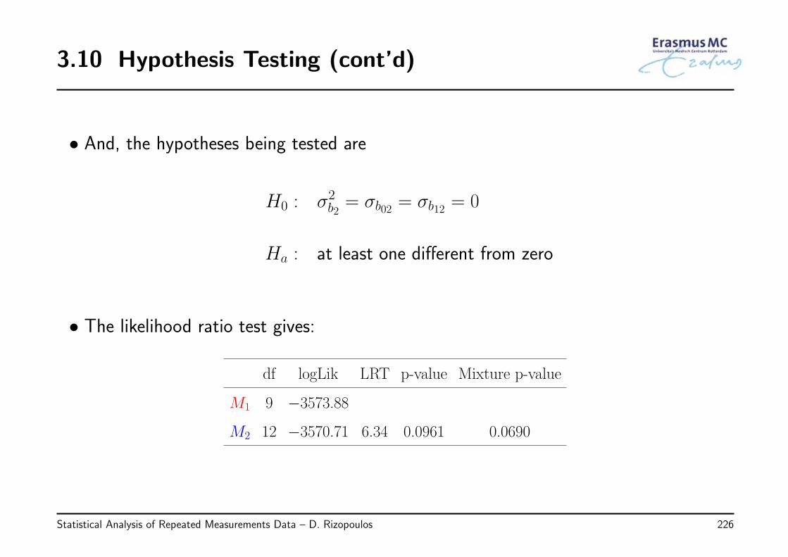
3.10 Hypothesis Testing (cont’d)
• And, the hypotheses being tested are
H0 : σ2b2= σb02 = σb12 = 0
Ha : at least one different from zero
• The likelihood ratio test gives:
df logLik LRT p-value Mixture p-value
M1 9 −3573.88
M2 12 −3570.71 6.34 0.0961 0.0690
Statistical Analysis of Repeated Measurements Data – D. Rizopoulos 226
3.10 Hypothesis Testing (cont’d)
• About the two p-values
◃ The first p-value is based on the classic χ2 distribution with degrees of freedomthe number of parameters being tested, i.e., in this case 3
◃ The second p-value is based on the mixture of χ2 distributions with 3 degrees offreedom (i.e., the classic one) and 2 degrees of freedom (the number ofparameters not on the boundary under H0), respectively
• We observe that the classic p-value is more conservative
◃ as we have seen in the previous section (see pp.216), when choosing the appropriaterandom effects we should be more liberal, and hence the mixture of χ2
distribution is to be preferred
Statistical Analysis of Repeated Measurements Data – D. Rizopoulos 227
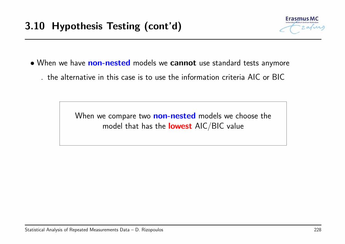
3.10 Hypothesis Testing (cont’d)
• When we have non-nested models we cannot use standard tests anymore
◃ the alternative in this case is to use the information criteria AIC or BIC
When we compare two non-nested models we choose themodel that has the lowest AIC/BIC value
Statistical Analysis of Repeated Measurements Data – D. Rizopoulos 228
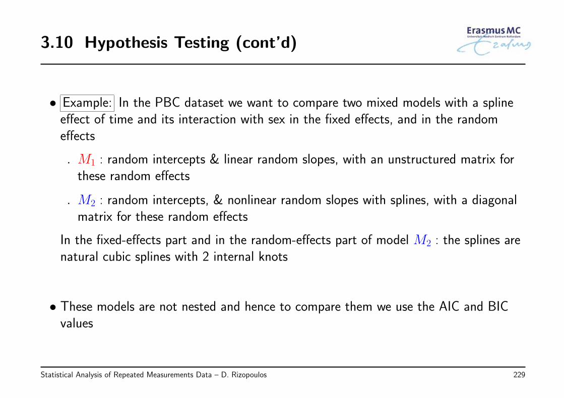
3.10 Hypothesis Testing (cont’d)
• Example: In the PBC dataset we want to compare two mixed models with a splineeffect of time and its interaction with sex in the fixed effects, and in the randomeffects
◃ M1 : random intercepts & linear random slopes, with an unstructured matrix forthese random effects
◃ M2 : random intercepts, & nonlinear random slopes with splines, with a diagonalmatrix for these random effects
In the fixed-effects part and in the random-effects part of model M2 : the splines arenatural cubic splines with 2 internal knots
• These models are not nested and hence to compare them we use the AIC and BICvalues
Statistical Analysis of Repeated Measurements Data – D. Rizopoulos 229
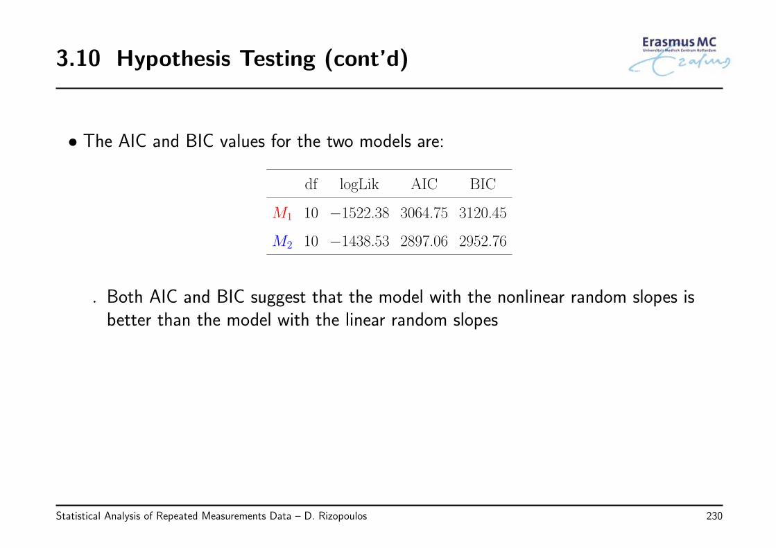
3.10 Hypothesis Testing (cont’d)
• The AIC and BIC values for the two models are:
df logLik AIC BIC
M1 10 −1522.38 3064.75 3120.45
M2 10 −1438.53 2897.06 2952.76
◃ Both AIC and BIC suggest that the model with the nonlinear random slopes isbetter than the model with the linear random slopes
Statistical Analysis of Repeated Measurements Data – D. Rizopoulos 230
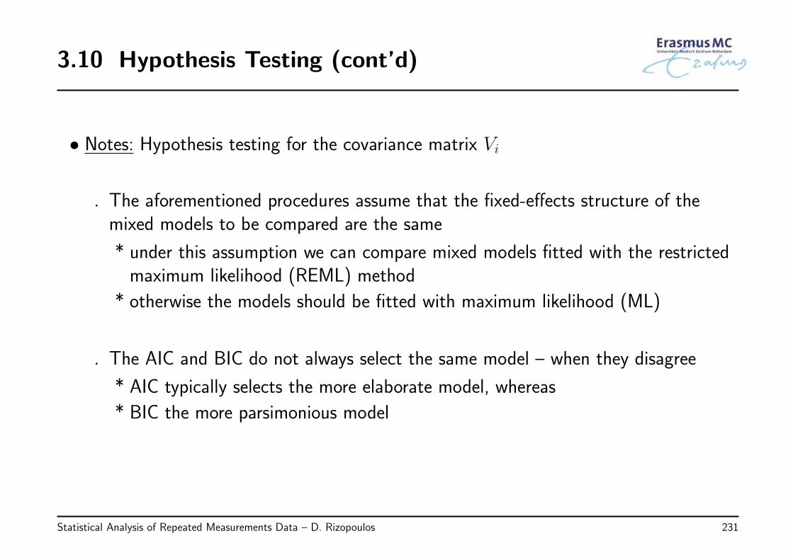
3.10 Hypothesis Testing (cont’d)
• Notes: Hypothesis testing for the covariance matrix Vi
◃ The aforementioned procedures assume that the fixed-effects structure of themixed models to be compared are the same
* under this assumption we can compare mixed models fitted with the restrictedmaximum likelihood (REML) method
* otherwise the models should be fitted with maximum likelihood (ML)
◃ The AIC and BIC do not always select the same model – when they disagree
* AIC typically selects the more elaborate model, whereas
* BIC the more parsimonious model
Statistical Analysis of Repeated Measurements Data – D. Rizopoulos 231
3.10 Hypothesis Testing (cont’d)
• Hypothesis testing for the regression coefficients β: We assume that first asuitable choice for the covariance matrix has been made
• In the majority of the cases we compare nested models, and hence standard tests canbe used
• We distinguish between two cases
◃ tests for individual coefficients
◃ tests for groups of coefficients
Statistical Analysis of Repeated Measurements Data – D. Rizopoulos 232
3.10 Hypothesis Testing (cont’d)
• Everything works in the same manner as we have seen for marginal models inChapter 2 (see pp.108–111)
◃ hence, we are not going to repeat the details here
• Example: We have fitted the following model to the Prothro dataset:
Statistical Analysis of Repeated Measurements Data – D. Rizopoulos 233
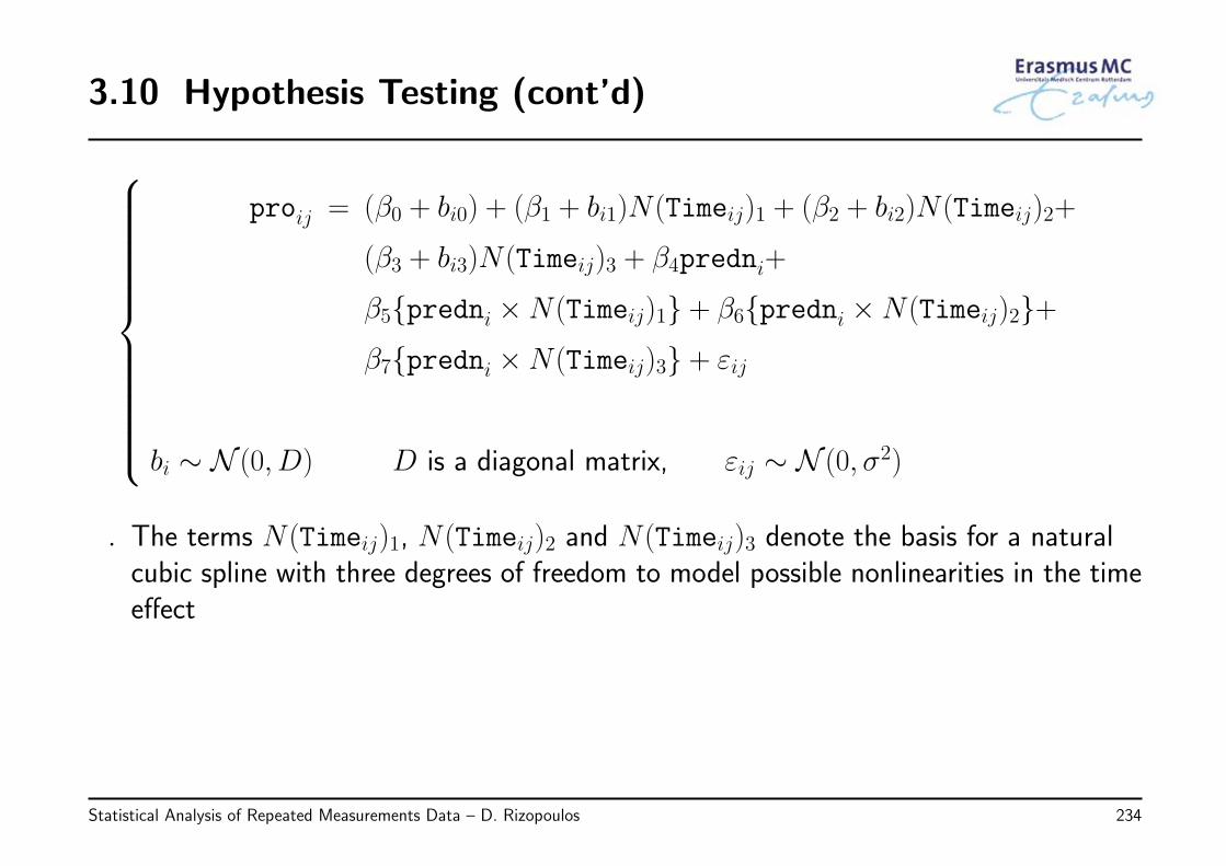
3.10 Hypothesis Testing (cont’d)
proij = (β0 + bi0) + (β1 + bi1)N(Timeij)1 + (β2 + bi2)N(Timeij)2+
(β3 + bi3)N(Timeij)3 + β4predni+
β5{predni ×N(Timeij)1} + β6{predni ×N(Timeij)2}+β7{predni ×N(Timeij)3} + εij
bi ∼ N (0, D) D is a diagonal matrix, εij ∼ N (0, σ2)
◃ The terms N(Timeij)1, N(Timeij)2 and N(Timeij)3 denote the basis for a naturalcubic spline with three degrees of freedom to model possible nonlinearities in the timeeffect
Statistical Analysis of Repeated Measurements Data – D. Rizopoulos 234
3.10 Hypothesis Testing (cont’d)
• We are interested in
◃ the main effect of treatment,
◃ the overall effect of time, and
◃ the overall effect of treatment (i.e., main effect + interactions)
• Under the postulated model the main effect of treatment is given by parameter β4,i.e.,
H0 : β4 = 0
Ha : β4 = 0
• The output of the model gives: . . .
Statistical Analysis of Repeated Measurements Data – D. Rizopoulos 235
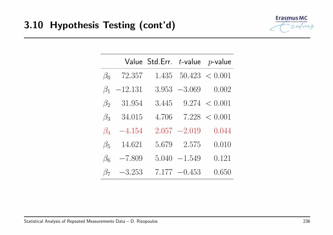
3.10 Hypothesis Testing (cont’d)
Value Std.Err. t-value p-value
β0 72.357 1.435 50.423 < 0.001
β1 −12.131 3.953 −3.069 0.002
β2 31.954 3.445 9.274 < 0.001
β3 34.015 4.706 7.228 < 0.001
β4 −4.154 2.057 −2.019 0.044
β5 14.621 5.679 2.575 0.010
β6 −7.809 5.040 −1.549 0.121
β7 −3.253 7.177 −0.453 0.650
Statistical Analysis of Repeated Measurements Data – D. Rizopoulos 236
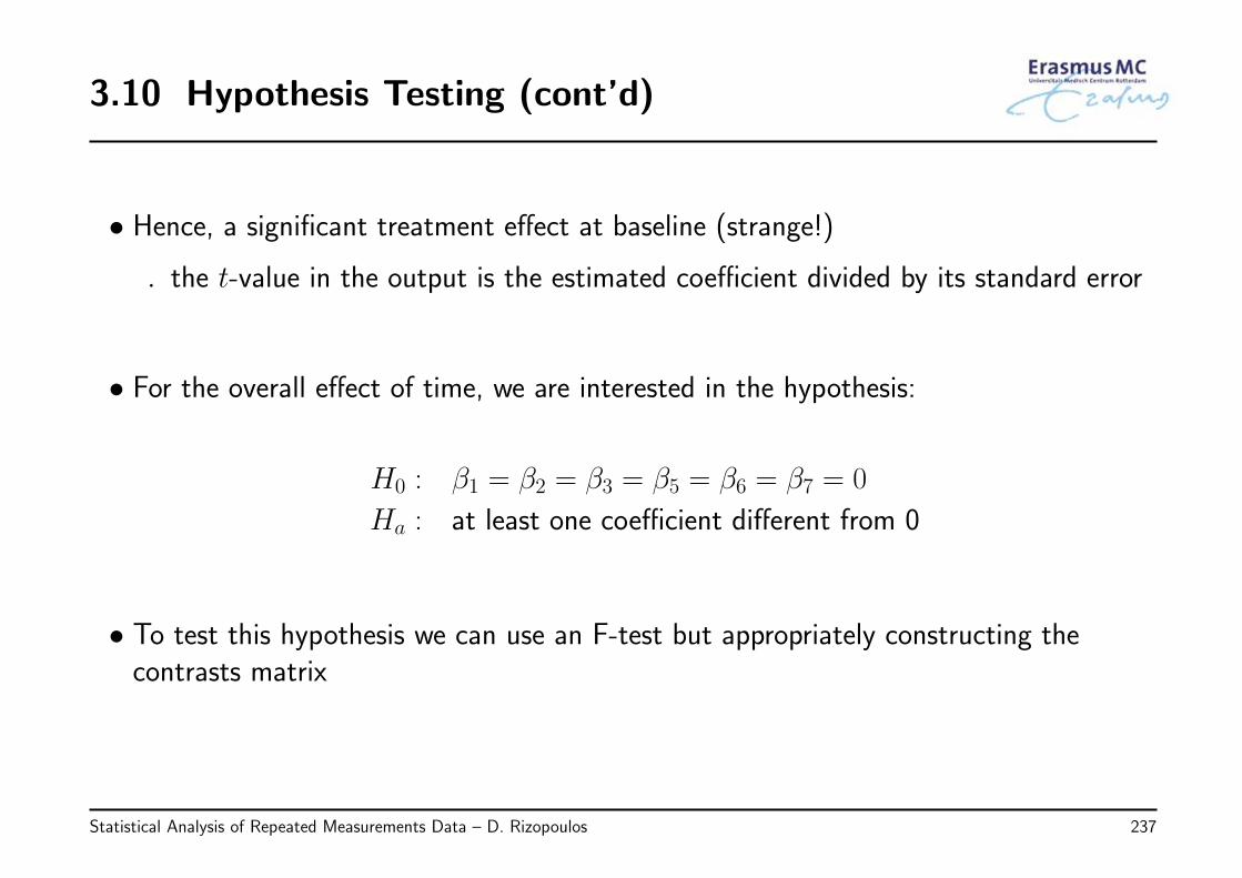
3.10 Hypothesis Testing (cont’d)
• Hence, a significant treatment effect at baseline (strange!)
◃ the t-value in the output is the estimated coefficient divided by its standard error
• For the overall effect of time, we are interested in the hypothesis:
H0 : β1 = β2 = β3 = β5 = β6 = β7 = 0
Ha : at least one coefficient different from 0
• To test this hypothesis we can use an F-test but appropriately constructing thecontrasts matrix
Statistical Analysis of Repeated Measurements Data – D. Rizopoulos 237
3.10 Hypothesis Testing (cont’d)
• We obtain
F -value df1 df2 p-value
23.555 6 1939 < 0.0001
◃ Hence, a significant overall time effect
Statistical Analysis of Repeated Measurements Data – D. Rizopoulos 238
3.10 Hypothesis Testing (cont’d)
• For the overall treatment effect, we obtain the hypothesis:
H0 : β4 = β5 = β6 = β7 = 0
Ha : at least one coefficient different from 0
• This cannot be tested with an F-test because of technical reasons
◃ the denominator degrees of freedom are not the same for the main effect and theterms involving time
• As an alternative we can use the likelihood ratio test
◃ i.e., we compare the model we fitted with the model that only has the nonlineareffect of time in the fixed effects
Statistical Analysis of Repeated Measurements Data – D. Rizopoulos 239
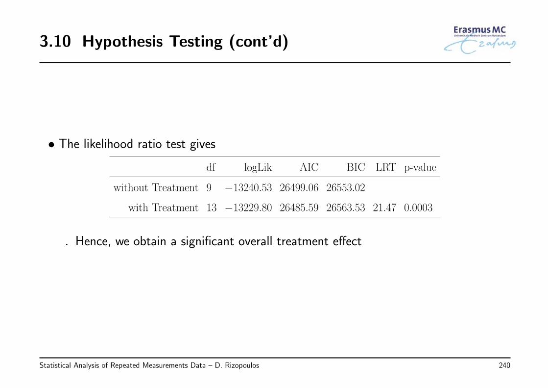
3.10 Hypothesis Testing (cont’d)
• The likelihood ratio test gives
df logLik AIC BIC LRT p-value
without Treatment 9 −13240.53 26499.06 26553.02
with Treatment 13 −13229.80 26485.59 26563.53 21.47 0.0003
◃ Hence, we obtain a significant overall treatment effect
Statistical Analysis of Repeated Measurements Data – D. Rizopoulos 240
3.11 Residuals
• As we have similarly done for marginal models in Chapter 2, before extractingconclusions from mixed models, we will first need to validate the underlyingassumptions they make
• To do this we can use the residuals of the model
• In the setting of mixed models we have two types of residuals
◃ Marginal residuals: These are based on the implied marginal model behind a linearmixed model (see pp.160)
◃ Conditional residuals: These are based on the hierarchical representation of themixed model and utilize the empirical Bayes estimates of the random effects (see
pp.174)
Statistical Analysis of Repeated Measurements Data – D. Rizopoulos 241
3.11 Residuals (cont’d)
• The exact definitions are as follows:
◃ Marginal residuals:yi = Xiβ + ε∗i , ε∗i ∼ N (0, ZiDZ⊤
i + σ2Ini)
rmargi = yi −Xiβ
◃ These residuals predict the marginal errors ε∗i
◃ They can be used to
* investigate misspecification of the mean structure Xiβ
* validate the assumptions for the within-subjects covariance structureZiDZ⊤
i + σ2Ini
Statistical Analysis of Repeated Measurements Data – D. Rizopoulos 242
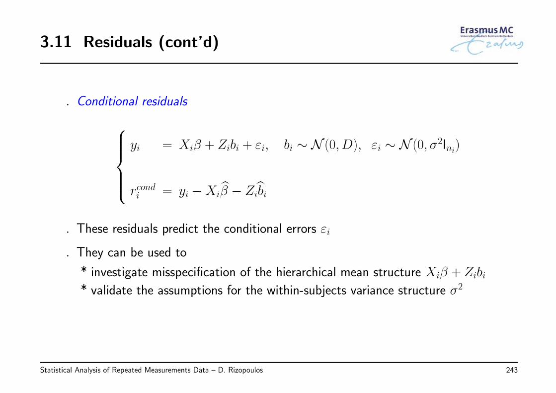
3.11 Residuals (cont’d)
◃ Conditional residualsyi = Xiβ + Zibi + εi, bi ∼ N (0, D), εi ∼ N (0, σ2Ini)
rcondi = yi −Xiβ − Zibi
◃ These residuals predict the conditional errors εi
◃ They can be used to
* investigate misspecification of the hierarchical mean structure Xiβ + Zibi* validate the assumptions for the within-subjects variance structure σ2
Statistical Analysis of Repeated Measurements Data – D. Rizopoulos 243
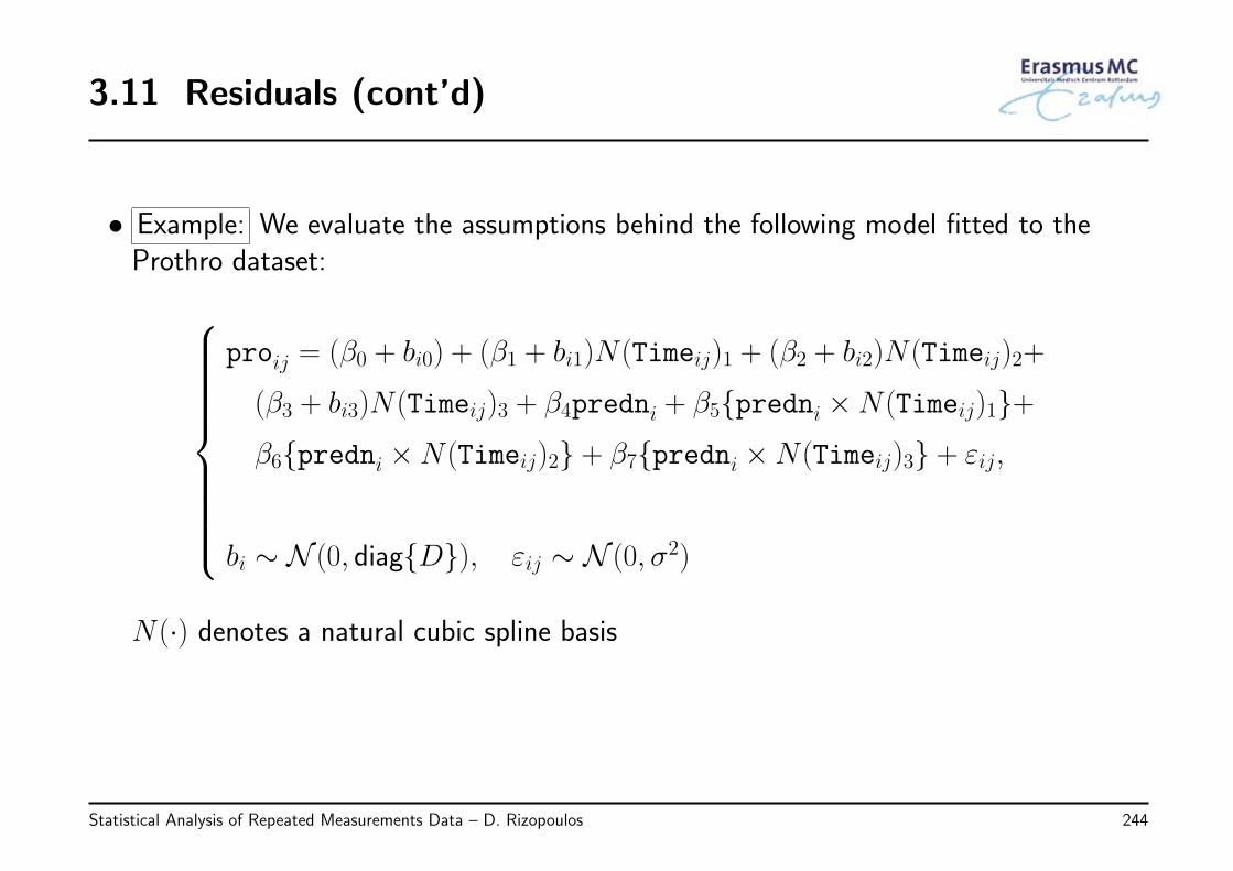
3.11 Residuals (cont’d)
• Example: We evaluate the assumptions behind the following model fitted to theProthro dataset:
proij = (β0 + bi0) + (β1 + bi1)N(Timeij)1 + (β2 + bi2)N(Timeij)2+
(β3 + bi3)N(Timeij)3 + β4predni + β5{predni ×N(Timeij)1}+β6{predni ×N(Timeij)2} + β7{predni ×N(Timeij)3} + εij,
bi ∼ N (0, diag{D}), εij ∼ N (0, σ2)
N(·) denotes a natural cubic spline basis
Statistical Analysis of Repeated Measurements Data – D. Rizopoulos 244
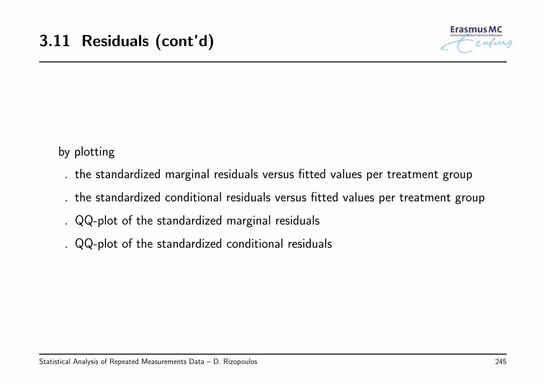
3.11 Residuals (cont’d)
by plotting
◃ the standardized marginal residuals versus fitted values per treatment group
◃ the standardized conditional residuals versus fitted values per treatment group
◃ QQ-plot of the standardized marginal residuals
◃ QQ-plot of the standardized conditional residuals
Statistical Analysis of Repeated Measurements Data – D. Rizopoulos 245
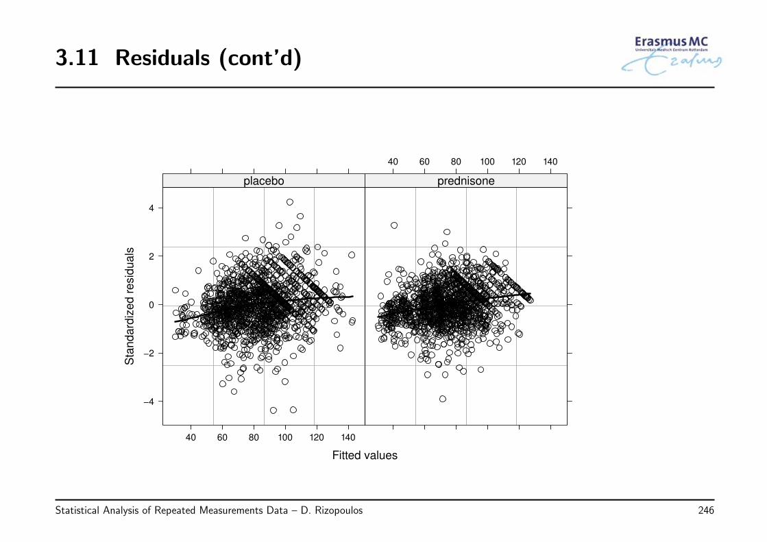
3.11 Residuals (cont’d)
Fitted values
Sta
nd
ard
ize
d r
esid
ua
ls
−4
−2
0
2
4
40 60 80 100 120 140
placebo
40 60 80 100 120 140
prednisone
Statistical Analysis of Repeated Measurements Data – D. Rizopoulos 246
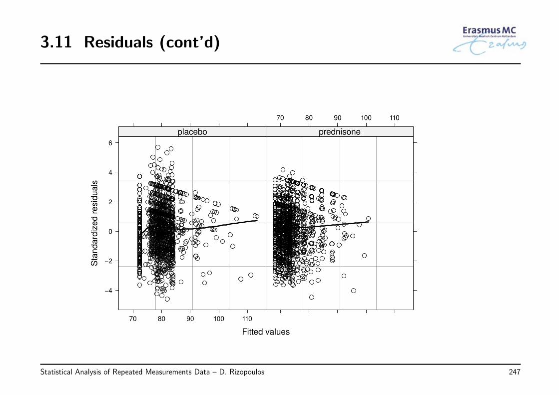
3.11 Residuals (cont’d)
Fitted values
Sta
nd
ard
ize
d r
esid
ua
ls
−4
−2
0
2
4
6
70 80 90 100 110
placebo
70 80 90 100 110
prednisone
Statistical Analysis of Repeated Measurements Data – D. Rizopoulos 247
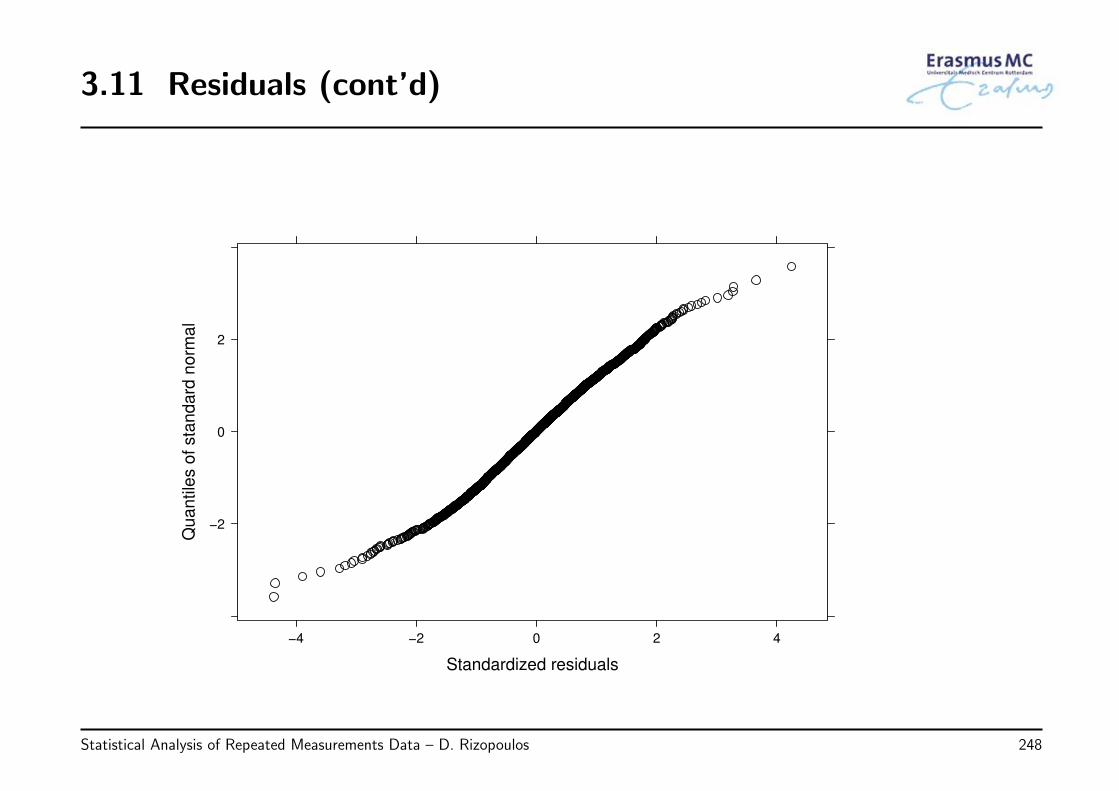
3.11 Residuals (cont’d)
Standardized residuals
Qu
an
tile
s o
f sta
nda
rd n
orm
al
−2
0
2
−4 −2 0 2 4
Statistical Analysis of Repeated Measurements Data – D. Rizopoulos 248
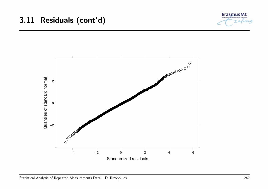
3.11 Residuals (cont’d)
Standardized residuals
Qu
an
tile
s o
f sta
nda
rd n
orm
al
−2
0
2
−4 −2 0 2 4 6
Statistical Analysis of Repeated Measurements Data – D. Rizopoulos 249
3.11 Residuals (cont’d)
• Observations
◃ the plots of the residuals versus the fitted values do show a slightly systematicbehavior
◃ the QQ-plots do not show big discrepancies from normality
Statistical Analysis of Repeated Measurements Data – D. Rizopoulos 250
3.12 Review of Key Points
• Mixed effects models constitute an alternative modeling framework for analyzinggrouped/clustered data
◃ basic idea: sample units in the same group/cluster share the same random effects
◃ the random effects are unobserved variables that induce correlation
• From a practical viewpoint, mixed models provide a more flexible framework to modelcorrelations when
◃ we have unbalanced data and/or
◃ the correlation structure has a complicated form (e.g., multilevel designs)
Statistical Analysis of Repeated Measurements Data – D. Rizopoulos 251
3.12 Review of Key Points (cont’d)
• The random effects can be estimated using empirical Bayes methodology
◃ mixed models provide subject-specific predictions that are more accurate thanmarginal predictions
• Mixed models can be extended to include correlated error terms
◃ this is in the same spirit as the marginal models of Chapter 2
◃ however, this extension often makes the model computationally unstable
Statistical Analysis of Repeated Measurements Data – D. Rizopoulos 252
3.12 Review of Key Points (cont’d)
• Hypothesis testing
◃ for the covariance structure and for nested models likelihood ratio tests are mostoften used, for non-nested models AIC/BIC
◃ for the mean structure t and F tests with appropriate degrees of freedom
• Residuals
◃ standard residuals plots are used to check the model assumptions
◃ marginal and conditional residuals available
Statistical Analysis of Repeated Measurements Data – D. Rizopoulos 253
Chapter 4
Marginal Models for Discrete Data
Statistical Analysis of Repeated Measurements Data – D. Rizopoulos 254
4.1 Review of Generalized Linear Models
• So far we have concentrated on continuous/normal repeated measurements data
◃ serum bilirubin and serum cholesterol in the PBC dataset
◃ CD4 cell counts in the AIDS dataset
◃ prothrombin time in the Prothro dataset
However often we may want to analyze other types ofrepeatedly measured outcomes that are not normally
distributed
Statistical Analysis of Repeated Measurements Data – D. Rizopoulos 255
4.1 Review of Generalized Linear Models (cont’d)
• Examples:
◃ in colon cancer studies the iFOBT test (presence or not of blood in stool) is usedto monitor patients ⇒ dichotomous data
◃ after a heart transplantation patients report their quality of life in frequentintervals, with the categories ‘Poor’, ‘Moderate’, ‘Good’ and ‘Very Good’ ⇒ordinal data
◃ in asthma studies often interest is in the number of asthma attacks patients havein a period of time ⇒ count data
◃ . . .
Statistical Analysis of Repeated Measurements Data – D. Rizopoulos 256
4.1 Review of Generalized Linear Models (cont’d)
• Suppose we have a dichotomous outcome Y measured cross-sectionally
◃ Example: The serum cholesterol levels from the PBC dataset at baseline (i.e.,time t = 0) that are higher than 210 mg/dL
• We are interested in making statistical inferences for this outcome, e.g.,
◃ is there any difference between placebo and D-penicillamine corrected for the ageand sex of the patients?
◃ which factors best predict serum cholesterol levels higher than 210 mg/dL?
⇓Generalized Linear Models
Statistical Analysis of Repeated Measurements Data – D. Rizopoulos 257
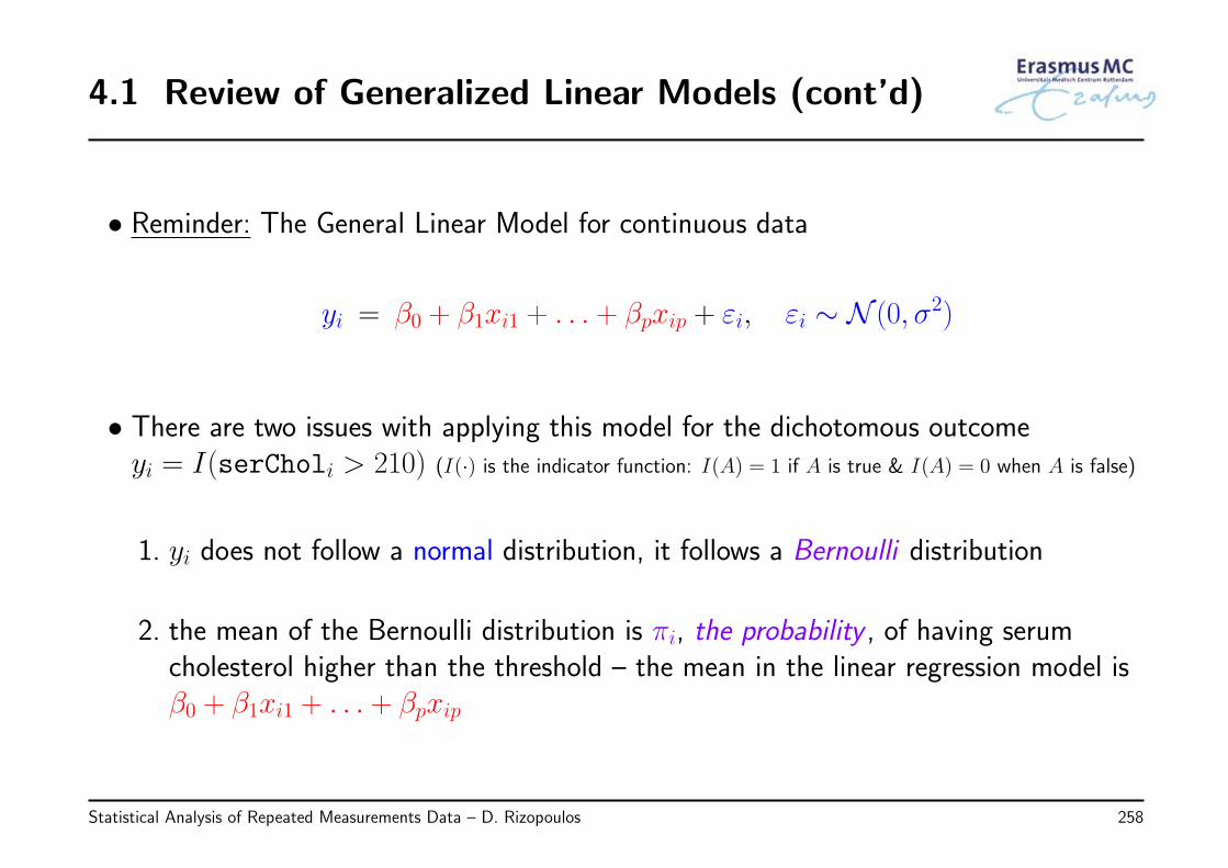
4.1 Review of Generalized Linear Models (cont’d)
• Reminder: The General Linear Model for continuous data
yi = β0 + β1xi1 + . . . + βpxip + εi, εi ∼ N (0, σ2)
• There are two issues with applying this model for the dichotomous outcomeyi = I(serCholi > 210) (I(·) is the indicator function: I(A) = 1 if A is true & I(A) = 0 when A is false)
1. yi does not follow a normal distribution, it follows a Bernoulli distribution
2. the mean of the Bernoulli distribution is πi, the probability , of having serumcholesterol higher than the threshold – the mean in the linear regression model isβ0 + β1xi1 + . . . + βpxip
Statistical Analysis of Repeated Measurements Data – D. Rizopoulos 258
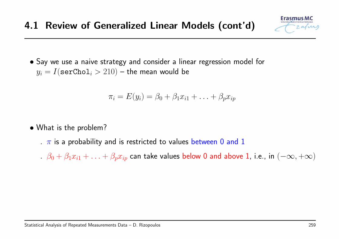
4.1 Review of Generalized Linear Models (cont’d)
• Say we use a naive strategy and consider a linear regression model foryi = I(serCholi > 210) – the mean would be
πi = E(yi) = β0 + β1xi1 + . . . + βpxip
• What is the problem?
◃ π is a probability and is restricted to values between 0 and 1
◃ β0 + β1xi1 + . . . + βpxip can take values below 0 and above 1, i.e., in (−∞,+∞)
Statistical Analysis of Repeated Measurements Data – D. Rizopoulos 259
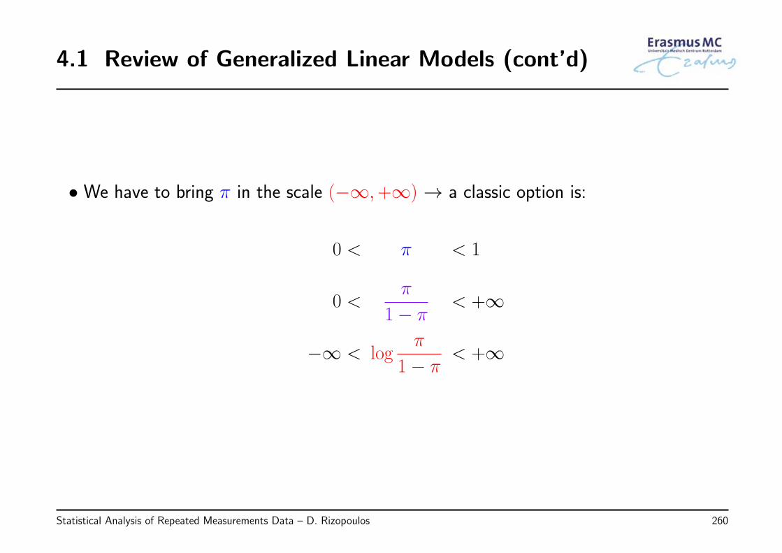
4.1 Review of Generalized Linear Models (cont’d)
• We have to bring π in the scale (−∞,+∞) → a classic option is:
0 < π < 1
0 <π
1− π< +∞
−∞ < logπ
1− π< +∞
Statistical Analysis of Repeated Measurements Data – D. Rizopoulos 260
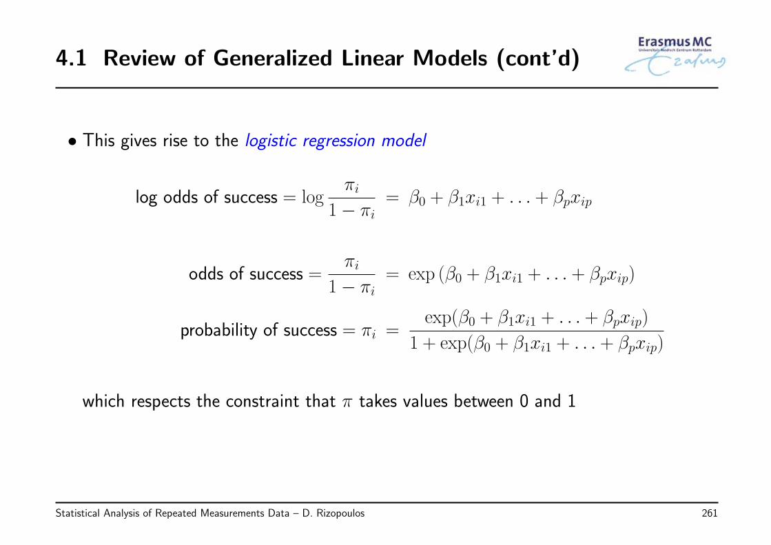
4.1 Review of Generalized Linear Models (cont’d)
• This gives rise to the logistic regression model
log odds of success = logπi
1− πi= β0 + β1xi1 + . . . + βpxip
odds of success =πi
1− πi= exp (β0 + β1xi1 + . . . + βpxip)
probability of success = πi =exp(β0 + β1xi1 + . . . + βpxip)
1 + exp(β0 + β1xi1 + . . . + βpxip)
which respects the constraint that π takes values between 0 and 1
Statistical Analysis of Repeated Measurements Data – D. Rizopoulos 261
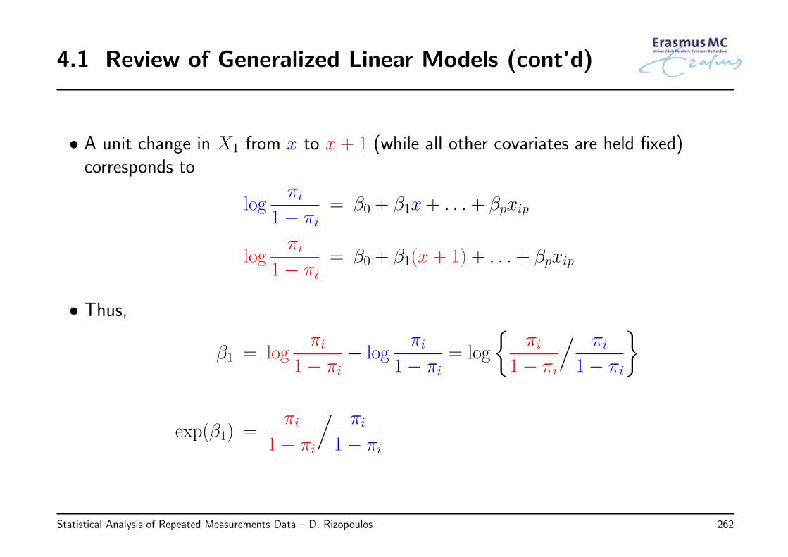
4.1 Review of Generalized Linear Models (cont’d)
• A unit change in X1 from x to x + 1 (while all other covariates are held fixed)corresponds to
logπi
1− πi= β0 + β1x + . . . + βpxip
logπi
1− πi= β0 + β1(x + 1) + . . . + βpxip
• Thus,
β1 = logπi
1− πi− log
πi1− πi
= log
{πi
1− πi
/ πi1− πi
}
exp(β1) =πi
1− πi
/ πi1− πi
Statistical Analysis of Repeated Measurements Data – D. Rizopoulos 262
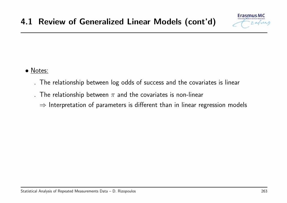
4.1 Review of Generalized Linear Models (cont’d)
• Notes:
◃ The relationship between log odds of success and the covariates is linear
◃ The relationship between π and the covariates is non-linear
⇒ Interpretation of parameters is different than in linear regression models
Statistical Analysis of Repeated Measurements Data – D. Rizopoulos 263
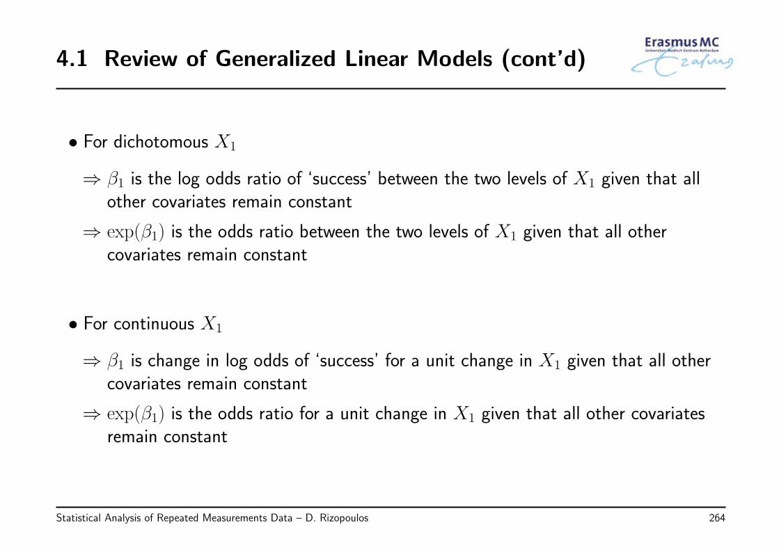
4.1 Review of Generalized Linear Models (cont’d)
• For dichotomous X1
⇒ β1 is the log odds ratio of ‘success’ between the two levels of X1 given that allother covariates remain constant
⇒ exp(β1) is the odds ratio between the two levels of X1 given that all othercovariates remain constant
• For continuous X1
⇒ β1 is change in log odds of ‘success’ for a unit change in X1 given that all othercovariates remain constant
⇒ exp(β1) is the odds ratio for a unit change in X1 given that all other covariatesremain constant
Statistical Analysis of Repeated Measurements Data – D. Rizopoulos 264
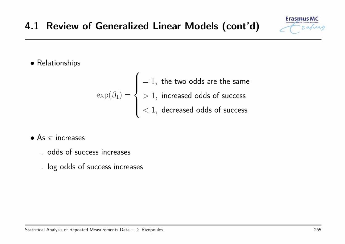
4.1 Review of Generalized Linear Models (cont’d)
• Relationships
exp(β1) =
= 1, the two odds are the same
> 1, increased odds of success
< 1, decreased odds of success
• As π increases
◃ odds of success increases
◃ log odds of success increases
Statistical Analysis of Repeated Measurements Data – D. Rizopoulos 265
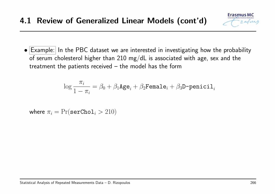
4.1 Review of Generalized Linear Models (cont’d)
• Example: In the PBC dataset we are interested in investigating how the probabilityof serum cholesterol higher than 210 mg/dL is associated with age, sex and thetreatment the patients received – the model has the form
logπi
1− πi= β0 + β1Agei + β2Femalei + β3D-penicili
where πi = Pr(serCholi > 210)
Statistical Analysis of Repeated Measurements Data – D. Rizopoulos 266
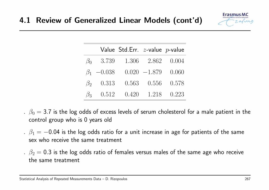
4.1 Review of Generalized Linear Models (cont’d)
Value Std.Err. z-value p-value
β0 3.739 1.306 2.862 0.004
β1 −0.038 0.020 −1.879 0.060
β2 0.313 0.563 0.556 0.578
β3 0.512 0.420 1.218 0.223
◃ β0 = 3.7 is the log odds of excess levels of serum cholesterol for a male patient in thecontrol group who is 0 years old
◃ β1 = −0.04 is the log odds ratio for a unit increase in age for patients of the samesex who receive the same treatment
◃ β2 = 0.3 is the log odds ratio of females versus males of the same age who receivethe same treatment
Statistical Analysis of Repeated Measurements Data – D. Rizopoulos 267
4.2 Generalized Estimating Equations
• We return our focus on repeated measurements data, namely, repeated categoricaldata
◃ we need to account for the correlations
• Reminder: In the marginal models for continuous multivariate data (Chapter 2) wetook account of the correlations by incorporating a correlation matrix in the errorterms
• For categorical data it is not straightforward to do that because there are no clearmultivariate analogues of the univariate distributions
◃ we will do something similar, not in the error terms but in the score equations
Statistical Analysis of Repeated Measurements Data – D. Rizopoulos 268
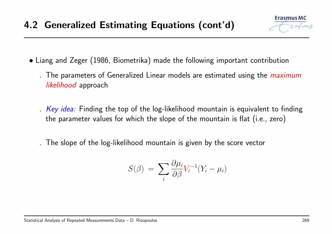
4.2 Generalized Estimating Equations (cont’d)
• Liang and Zeger (1986, Biometrika) made the following important contribution
◃ The parameters of Generalized Linear models are estimated using the maximumlikelihood approach
◃ Key idea: Finding the top of the log-likelihood mountain is equivalent to findingthe parameter values for which the slope of the mountain is flat (i.e., zero)
◃ The slope of the log-likelihood mountain is given by the score vector
S(β) =∑i
∂µi
∂βVi
−1(Yi − µi)
Statistical Analysis of Repeated Measurements Data – D. Rizopoulos 269
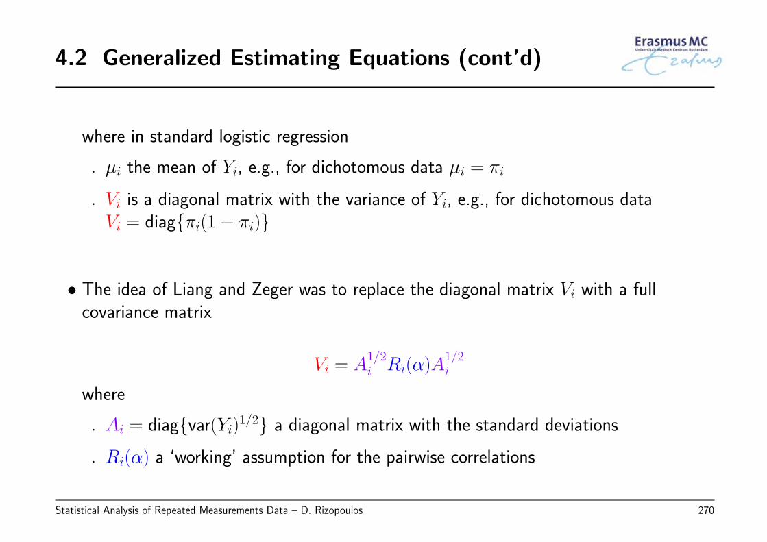
4.2 Generalized Estimating Equations (cont’d)
where in standard logistic regression
◃ µi the mean of Yi, e.g., for dichotomous data µi = πi
◃ Vi is a diagonal matrix with the variance of Yi, e.g., for dichotomous dataVi = diag{πi(1− πi)}
• The idea of Liang and Zeger was to replace the diagonal matrix Vi with a fullcovariance matrix
Vi = A1/2i Ri(α)A
1/2i
where
◃ Ai = diag{var(Yi)1/2} a diagonal matrix with the standard deviations
◃ Ri(α) a ‘working’ assumption for the pairwise correlations
Statistical Analysis of Repeated Measurements Data – D. Rizopoulos 270
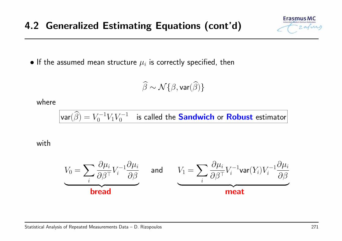
4.2 Generalized Estimating Equations (cont’d)
• If the assumed mean structure µi is correctly specified, then
β ∼ N{β, var(β)}
where
var(β) = V −10 V1V
−10 is called the Sandwich or Robust estimator
with
V0 =∑i
∂µi
∂β⊤V−1i
∂µi
∂β︸ ︷︷ ︸ and V1 =∑i
∂µi
∂β⊤V−1i var(Yi)V
−1i
∂µi
∂β︸ ︷︷ ︸bread meat
Statistical Analysis of Repeated Measurements Data – D. Rizopoulos 271
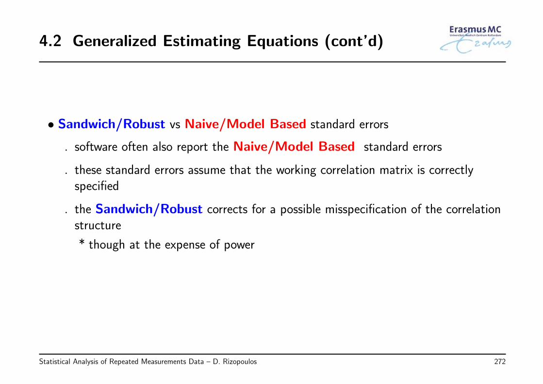
4.2 Generalized Estimating Equations (cont’d)
• Sandwich/Robust vs Naive/Model Based standard errors
◃ software often also report the Naive/Model Based standard errors
◃ these standard errors assume that the working correlation matrix is correctlyspecified
◃ the Sandwich/Robust corrects for a possible misspecification of the correlationstructure
* though at the expense of power
Statistical Analysis of Repeated Measurements Data – D. Rizopoulos 272
4.2 Generalized Estimating Equations (cont’d)
GEE is not a likelihood-based approach (i.e., a model)⇓
it is an estimation method
• No assumptions for the joint distribution of repeated measurements⇒ Semi-parametric approach
• Three components
1. Model for mean response E(Yi) = µi, e.g., binary data E(Yi) = πi
logπi
1− πi= β0 + β1xi1 + . . . + βpxip
Statistical Analysis of Repeated Measurements Data – D. Rizopoulos 273
4.2 Generalized Estimating Equations (cont’d)
2. Variance of Yi ⇒ follows from GLM assumption for each measurement, e.g.,binary data
var(Yi) = ϕπi(1− πi)
with ϕ a scale parameter that models over-dispersion
3. Pairwise correlations ⇒ we make a “working” assumption that possibly dependson parameters to be estimated
The mean and the correlations are separately defined!This is in contrast to the GLMMs we will see in the next chapter
Statistical Analysis of Repeated Measurements Data – D. Rizopoulos 274
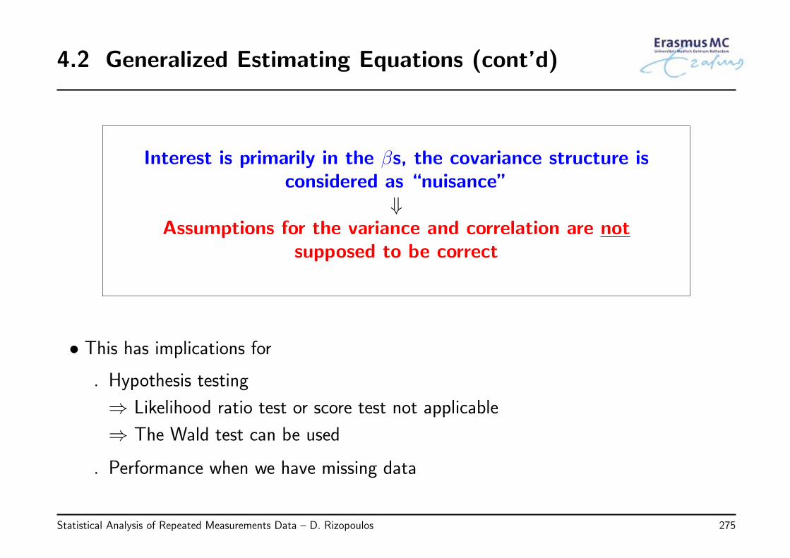
4.2 Generalized Estimating Equations (cont’d)
Interest is primarily in the βs, the covariance structure isconsidered as “nuisance”
⇓Assumptions for the variance and correlation are not
supposed to be correct
• This has implications for
◃ Hypothesis testing
⇒ Likelihood ratio test or score test not applicable
⇒ The Wald test can be used
◃ Performance when we have missing data
Statistical Analysis of Repeated Measurements Data – D. Rizopoulos 275
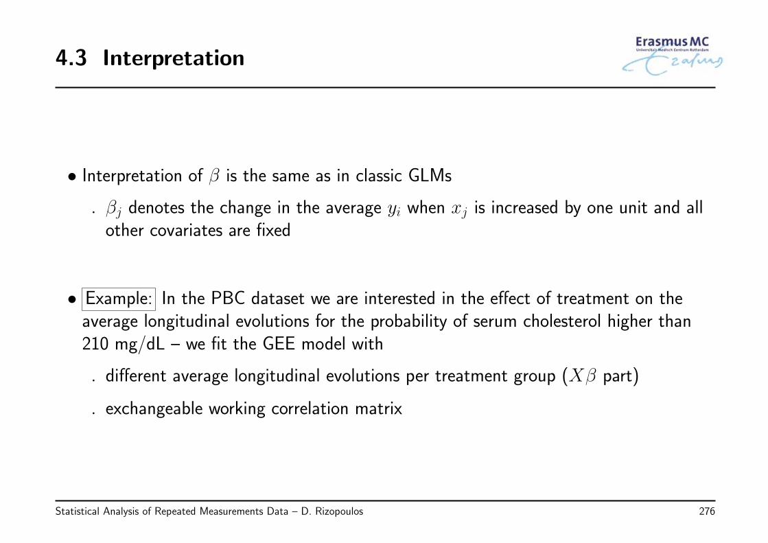
4.3 Interpretation
• Interpretation of β is the same as in classic GLMs
◃ βj denotes the change in the average yi when xj is increased by one unit and allother covariates are fixed
• Example: In the PBC dataset we are interested in the effect of treatment on theaverage longitudinal evolutions for the probability of serum cholesterol higher than210 mg/dL – we fit the GEE model with
◃ different average longitudinal evolutions per treatment group (Xβ part)
◃ exchangeable working correlation matrix
Statistical Analysis of Repeated Measurements Data – D. Rizopoulos 276
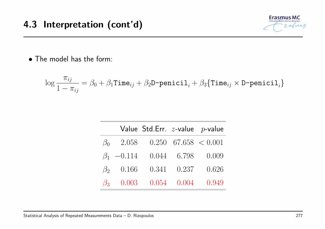
4.3 Interpretation (cont’d)
• The model has the form:
logπij
1− πij= β0 + β1Timeij + β2D-penicili + β3{Timeij × D-penicili}
Value Std.Err. z-value p-value
β0 2.058 0.250 67.658 < 0.001
β1 −0.114 0.044 6.798 0.009
β2 0.166 0.341 0.237 0.626
β3 0.003 0.054 0.004 0.949
Statistical Analysis of Repeated Measurements Data – D. Rizopoulos 277
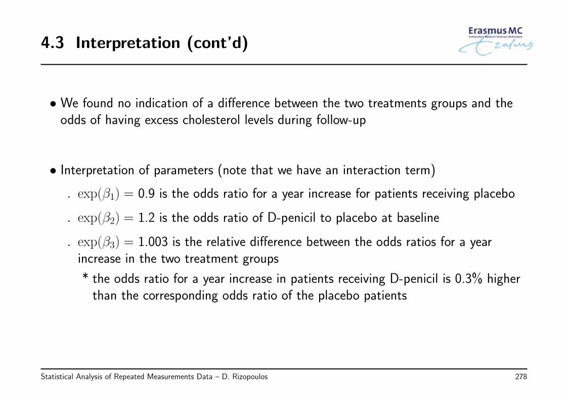
4.3 Interpretation (cont’d)
• We found no indication of a difference between the two treatments groups and theodds of having excess cholesterol levels during follow-up
• Interpretation of parameters (note that we have an interaction term)
◃ exp(β1) = 0.9 is the odds ratio for a year increase for patients receiving placebo
◃ exp(β2) = 1.2 is the odds ratio of D-penicil to placebo at baseline
◃ exp(β3) = 1.003 is the relative difference between the odds ratios for a yearincrease in the two treatment groups
* the odds ratio for a year increase in patients receiving D-penicil is 0.3% higherthan the corresponding odds ratio of the placebo patients
Statistical Analysis of Repeated Measurements Data – D. Rizopoulos 278
4.3 Interpretation (cont’d)
• As we have previously seen, to effectively communicate complex models we can useeffect plots
• Example: In the PBC dataset we are interested in the probability of having excessserum cholesterol levels
◃ we allow for nonlinear time and baseline age effects using natural cubic splineswith 3 degrees of freedom
◃ we also correct for treatment and gender
Statistical Analysis of Repeated Measurements Data – D. Rizopoulos 279
4.3 Interpretation (cont’d)
• The following two figures depict the relationship between
◃ the log odds of excess serum cholesterol level
◃ the probability of excess serum cholesterol level
for male and female patients receiving either the active drug or placebo, who are 49years old (in the app different ages can be selected)
Statistical Analysis of Repeated Measurements Data – D. Rizopoulos 280
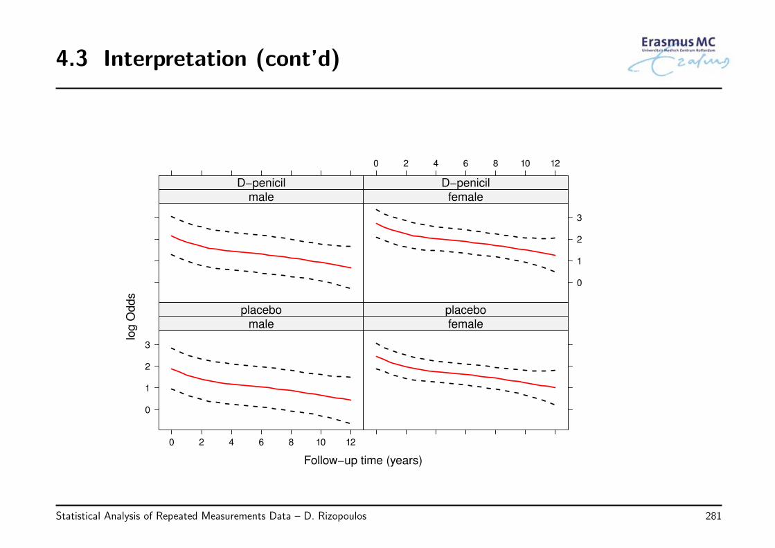
4.3 Interpretation (cont’d)
Follow−up time (years)
log
Odd
s
0
1
2
3
0 2 4 6 8 10 12
male
placebo
female
placebo
male
D−penicil
0 2 4 6 8 10 12
0
1
2
3
female
D−penicil
Statistical Analysis of Repeated Measurements Data – D. Rizopoulos 281
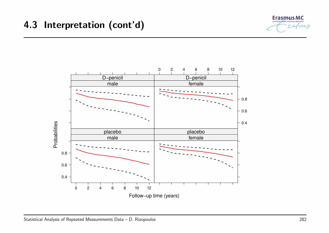
4.3 Interpretation (cont’d)
Follow−up time (years)
Pro
ba
bili
ties
0.4
0.6
0.8
0 2 4 6 8 10 12
male
placebo
female
placebo
male
D−penicil
0 2 4 6 8 10 12
0.4
0.6
0.8
female
D−penicil
Statistical Analysis of Repeated Measurements Data – D. Rizopoulos 282
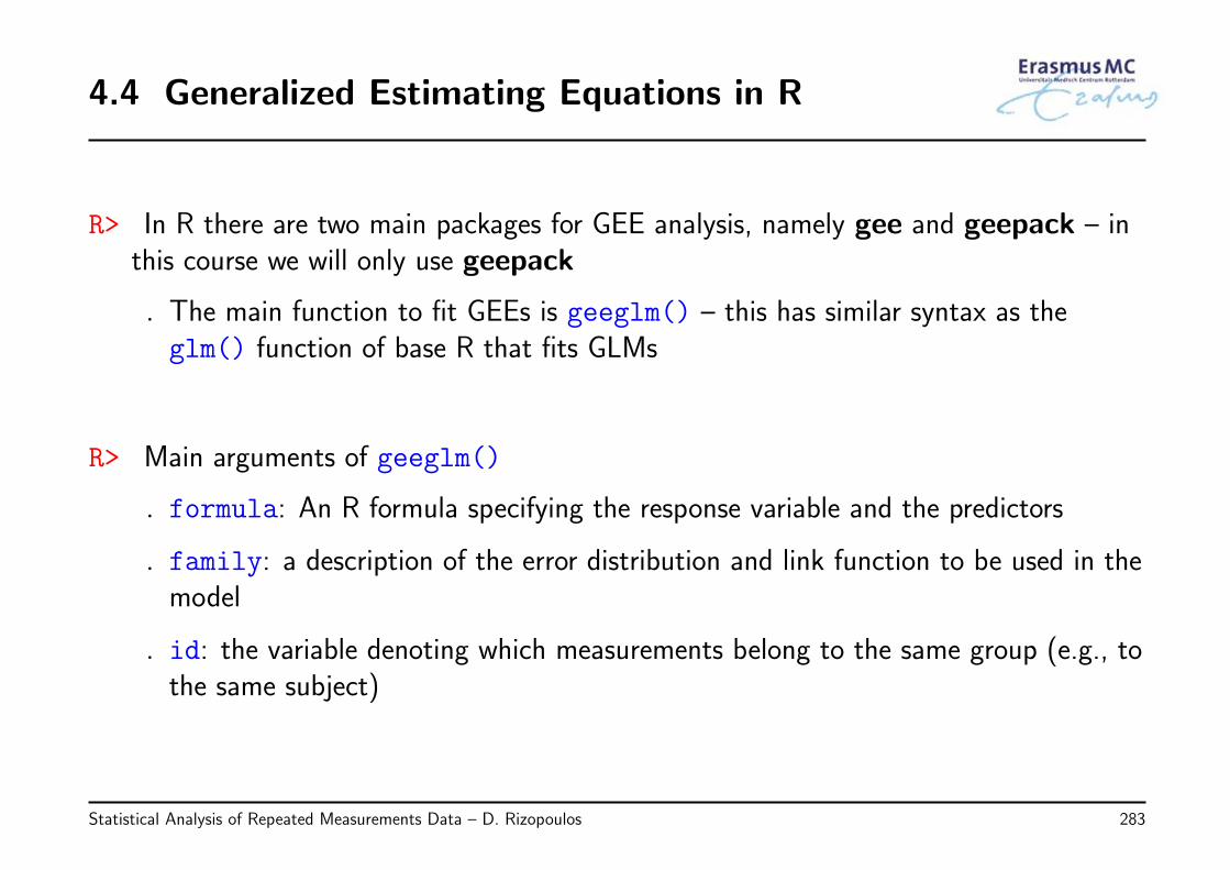
4.4 Generalized Estimating Equations in R
R> In R there are two main packages for GEE analysis, namely gee and geepack – inthis course we will only use geepack
◃ The main function to fit GEEs is geeglm() – this has similar syntax as theglm() function of base R that fits GLMs
R> Main arguments of geeglm()
◃ formula: An R formula specifying the response variable and the predictors
◃ family: a description of the error distribution and link function to be used in themodel
◃ id: the variable denoting which measurements belong to the same group (e.g., tothe same subject)
Statistical Analysis of Repeated Measurements Data – D. Rizopoulos 283
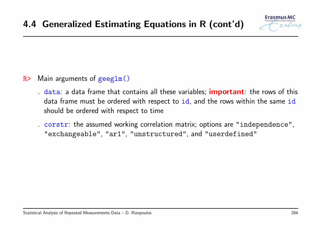
4.4 Generalized Estimating Equations in R (cont’d)
R> Main arguments of geeglm()
◃ data: a data frame that contains all these variables; important: the rows of thisdata frame must be ordered with respect to id, and the rows within the same idshould be ordered with respect to time
◃ corstr: the assumed working correlation matrix; options are "independence","exchangeable", "ar1", "unstructured", and "userdefined"
Statistical Analysis of Repeated Measurements Data – D. Rizopoulos 284
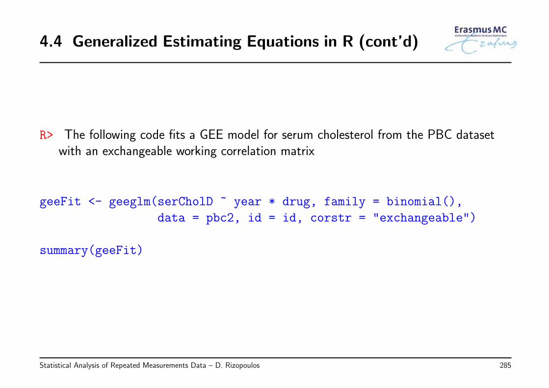
4.4 Generalized Estimating Equations in R (cont’d)
R> The following code fits a GEE model for serum cholesterol from the PBC datasetwith an exchangeable working correlation matrix
geeFit <- geeglm(serCholD ~ year * drug, family = binomial(),
data = pbc2, id = id, corstr = "exchangeable")
summary(geeFit)
Statistical Analysis of Repeated Measurements Data – D. Rizopoulos 285
4.5 Working Correlation Matrix
• As we have seen, the GEEs are a semiparametric approach
◃ using the sandwich estimator we obtain valid inferences even if the workingcorrelation matrix is misspecified
• Hence, one could wonder: Why not always use the sandwich estimator in order not tohave to care about the correlation structure?
◃ in other words, why do we need this course?
The sandwich estimator does have important limitations!
Statistical Analysis of Repeated Measurements Data – D. Rizopoulos 286
4.5 Working Correlation Matrix (cont’d)
• About the sandwich estimator:
◃ is based on asymptotic arguments ⇒ it only works for big samples
◃ more specifically, it works better under the following settings
* when the number of subjects is considerably larger than the number of repeatedmeasurements,
* balanced designs in which all subjects provide measurements at the same timepoints
* we do not have too many covariates (especially continuous)
• Therefore, the choice of the working correlation matrix is of particular importance
◃ this is why all statistical software offer several alternative options for this matrix
Statistical Analysis of Repeated Measurements Data – D. Rizopoulos 287
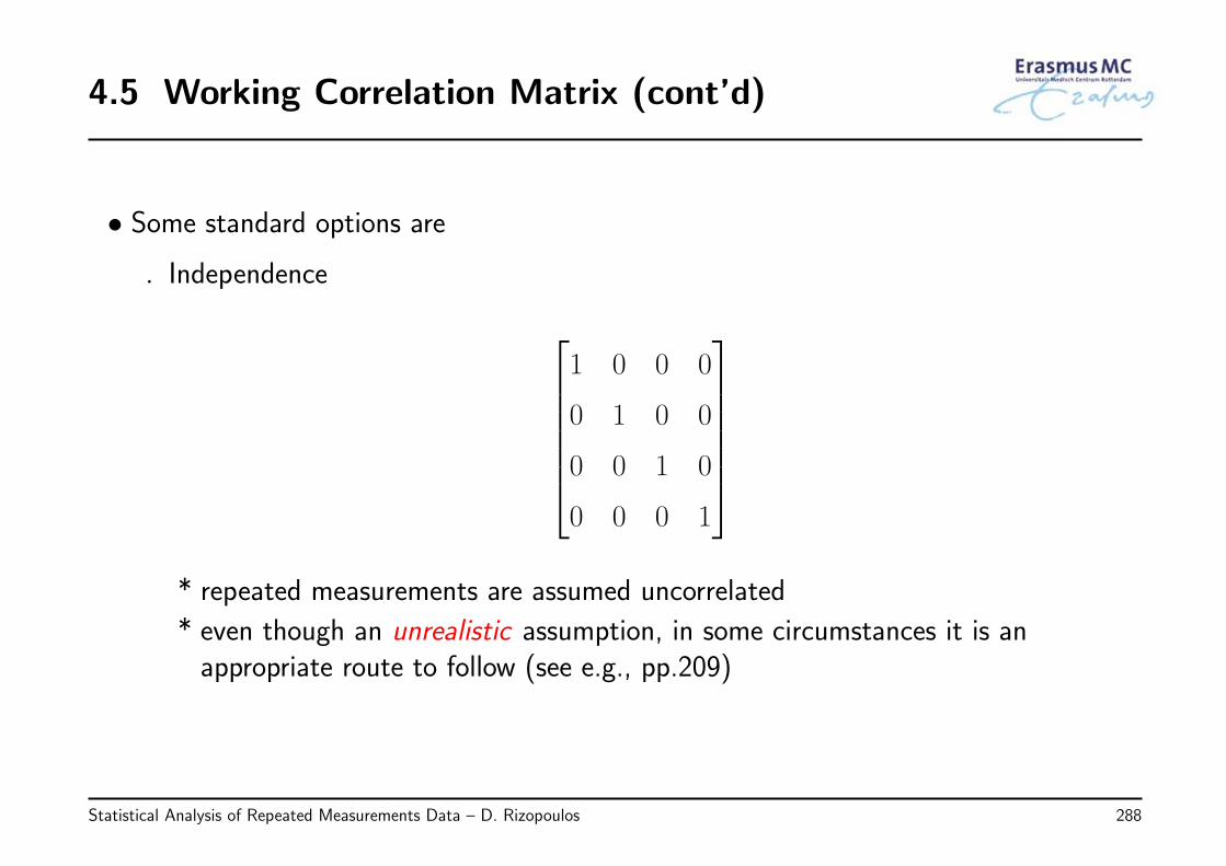
4.5 Working Correlation Matrix (cont’d)
• Some standard options are
◃ Independence
1 0 0 0
0 1 0 0
0 0 1 0
0 0 0 1
* repeated measurements are assumed uncorrelated
* even though an unrealistic assumption, in some circumstances it is anappropriate route to follow (see e.g., pp.209)
Statistical Analysis of Repeated Measurements Data – D. Rizopoulos 288
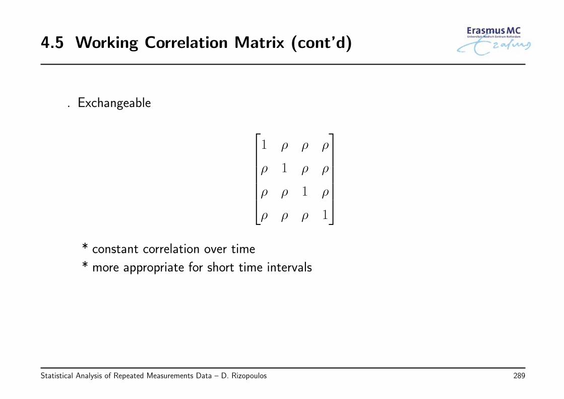
4.5 Working Correlation Matrix (cont’d)
◃ Exchangeable
1 ρ ρ ρ
ρ 1 ρ ρ
ρ ρ 1 ρ
ρ ρ ρ 1
* constant correlation over time
* more appropriate for short time intervals
Statistical Analysis of Repeated Measurements Data – D. Rizopoulos 289
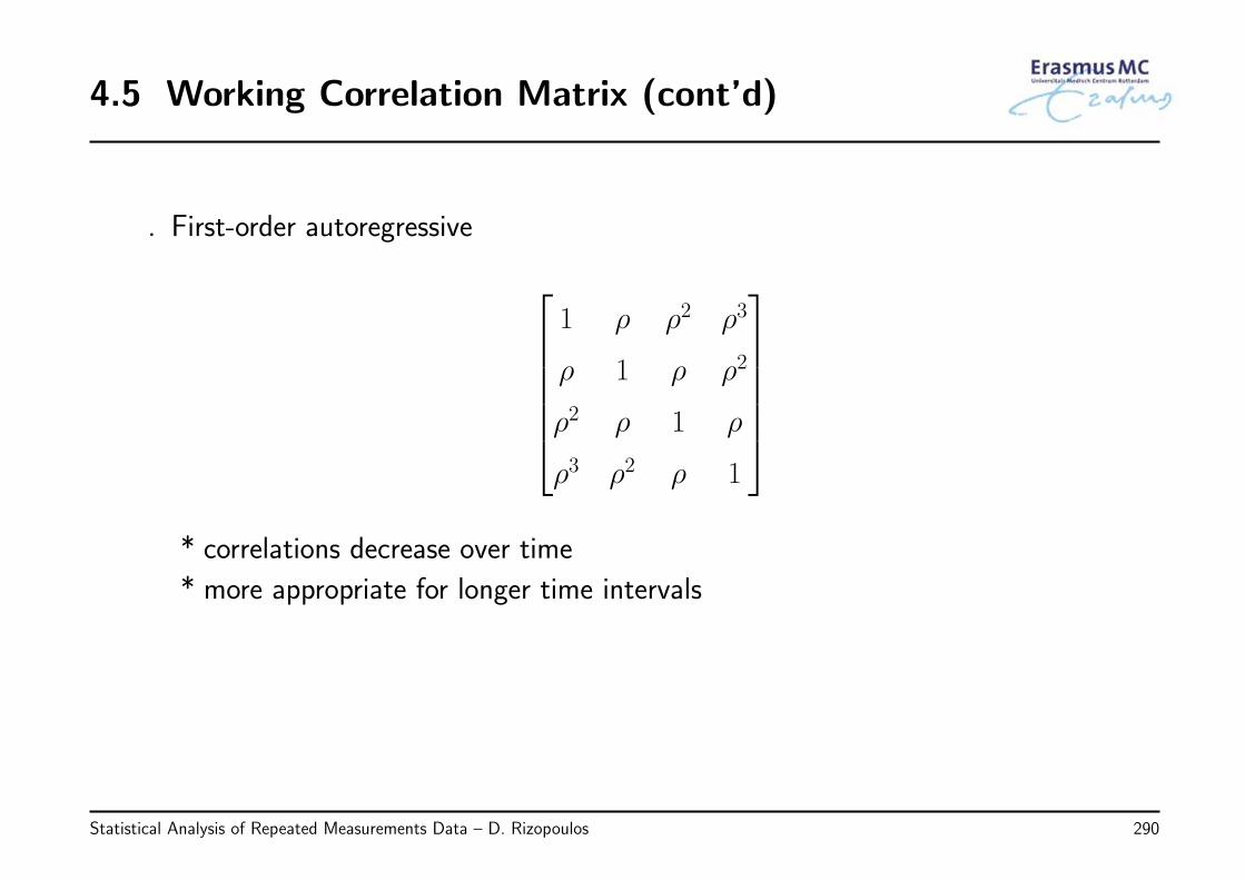
4.5 Working Correlation Matrix (cont’d)
◃ First-order autoregressive
1 ρ ρ2 ρ3
ρ 1 ρ ρ2
ρ2 ρ 1 ρ
ρ3 ρ2 ρ 1
* correlations decrease over time
* more appropriate for longer time intervals
Statistical Analysis of Repeated Measurements Data – D. Rizopoulos 290
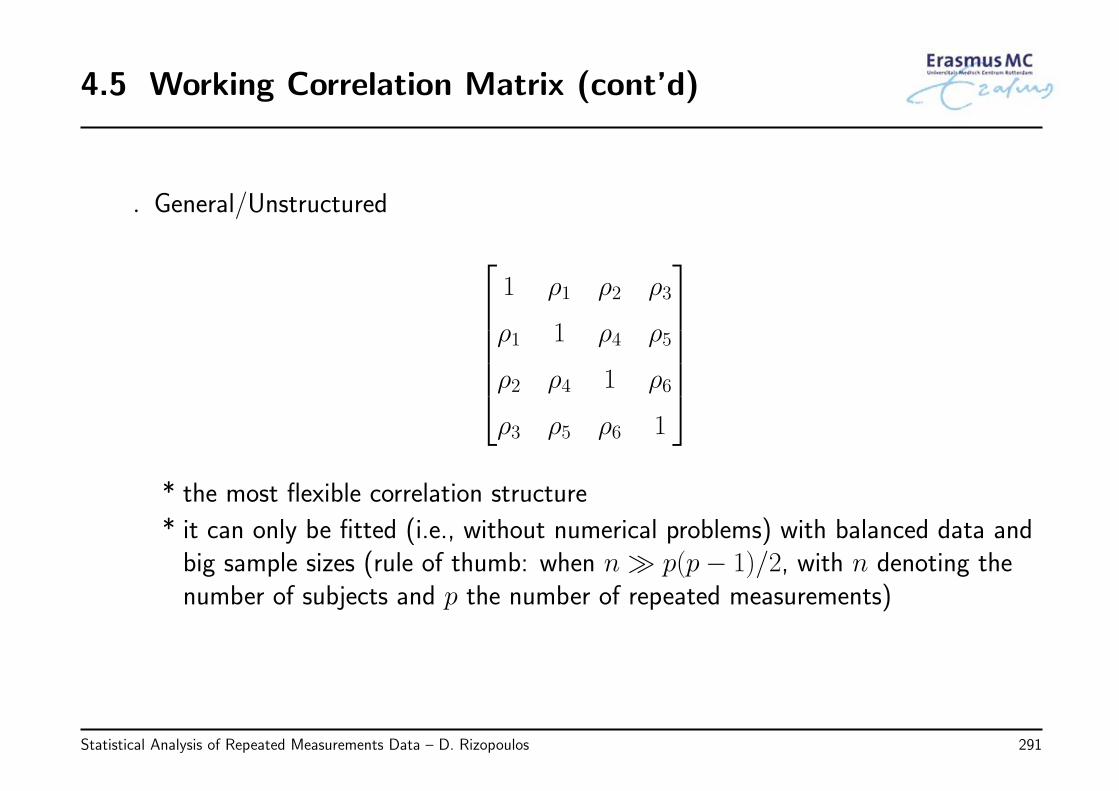
4.5 Working Correlation Matrix (cont’d)
◃ General/Unstructured
1 ρ1 ρ2 ρ3
ρ1 1 ρ4 ρ5
ρ2 ρ4 1 ρ6
ρ3 ρ5 ρ6 1
* the most flexible correlation structure
* it can only be fitted (i.e., without numerical problems) with balanced data andbig sample sizes (rule of thumb: when n ≫ p(p− 1)/2, with n denoting thenumber of subjects and p the number of repeated measurements)
Statistical Analysis of Repeated Measurements Data – D. Rizopoulos 291
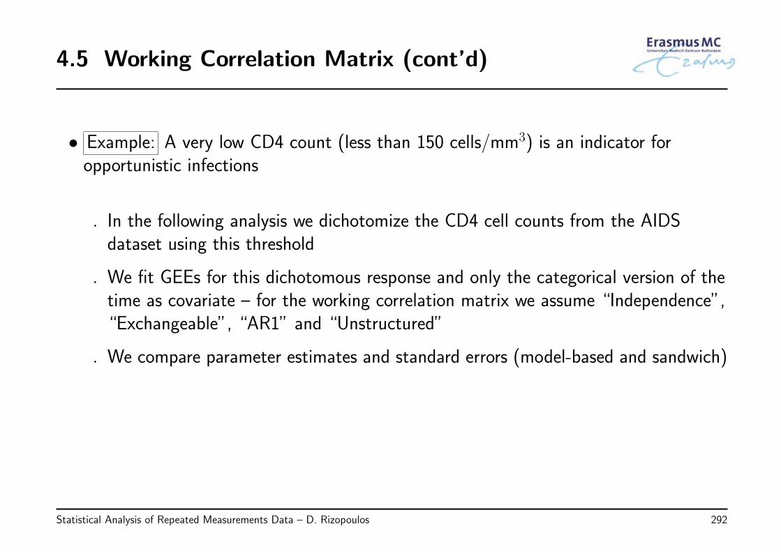
4.5 Working Correlation Matrix (cont’d)
• Example: A very low CD4 count (less than 150 cells/mm3) is an indicator foropportunistic infections
◃ In the following analysis we dichotomize the CD4 cell counts from the AIDSdataset using this threshold
◃ We fit GEEs for this dichotomous response and only the categorical version of thetime as covariate – for the working correlation matrix we assume “Independence”,“Exchangeable”, “AR1” and “Unstructured”
◃ We compare parameter estimates and standard errors (model-based and sandwich)
Statistical Analysis of Repeated Measurements Data – D. Rizopoulos 292
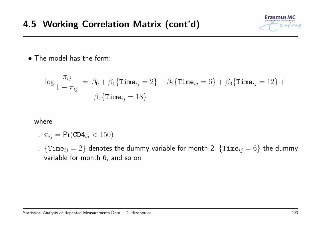
4.5 Working Correlation Matrix (cont’d)
• The model has the form:
logπij
1− πij= β0 + β1{Timeij = 2} + β2{Timeij = 6} + β3{Timeij = 12} +
β4{Timeij = 18}
where
◃ πij = Pr(CD4ij < 150)
◃ {Timeij = 2} denotes the dummy variable for month 2, {Timeij = 6} the dummyvariable for month 6, and so on
Statistical Analysis of Repeated Measurements Data – D. Rizopoulos 293
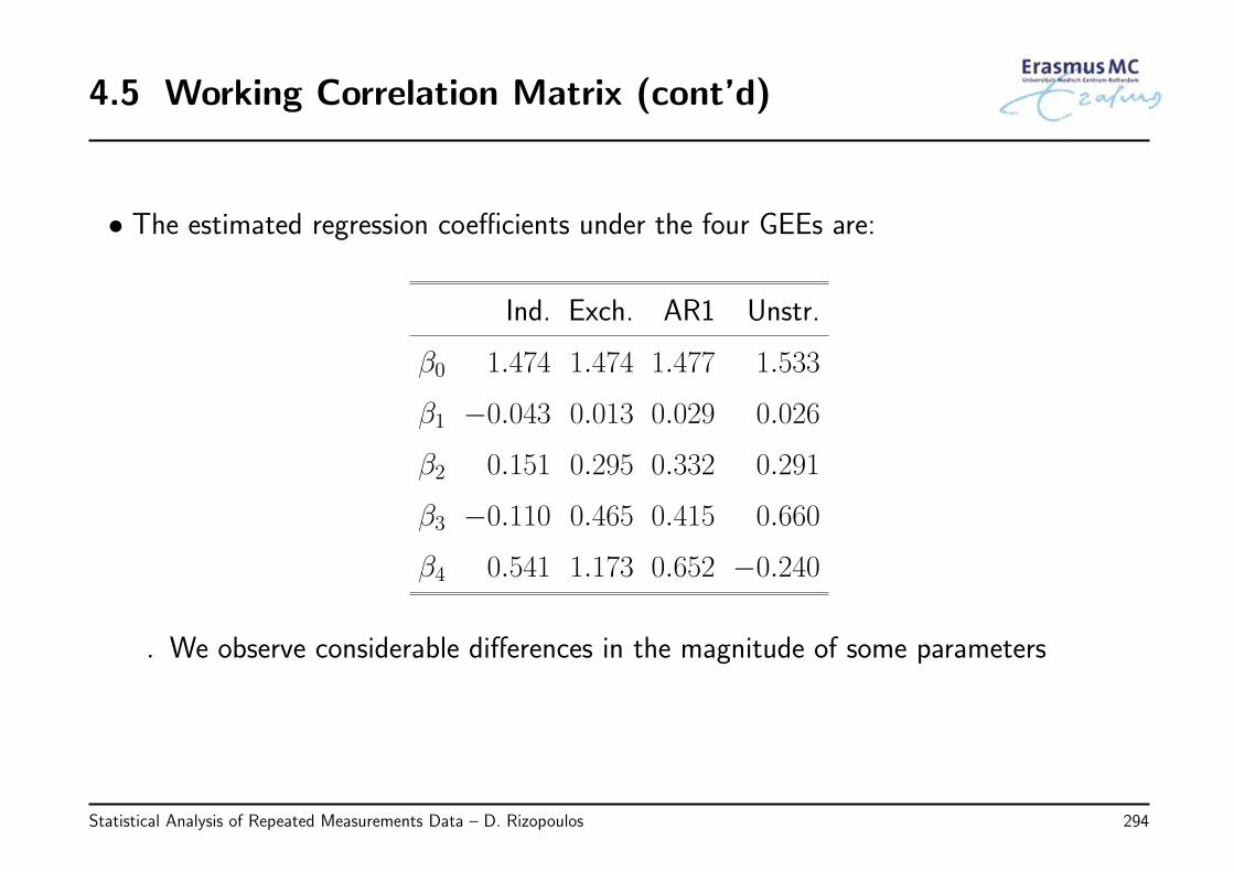
4.5 Working Correlation Matrix (cont’d)
• The estimated regression coefficients under the four GEEs are:
Ind. Exch. AR1 Unstr.
β0 1.474 1.474 1.477 1.533
β1 −0.043 0.013 0.029 0.026
β2 0.151 0.295 0.332 0.291
β3 −0.110 0.465 0.415 0.660
β4 0.541 1.173 0.652 −0.240
◃ We observe considerable differences in the magnitude of some parameters
Statistical Analysis of Repeated Measurements Data – D. Rizopoulos 294
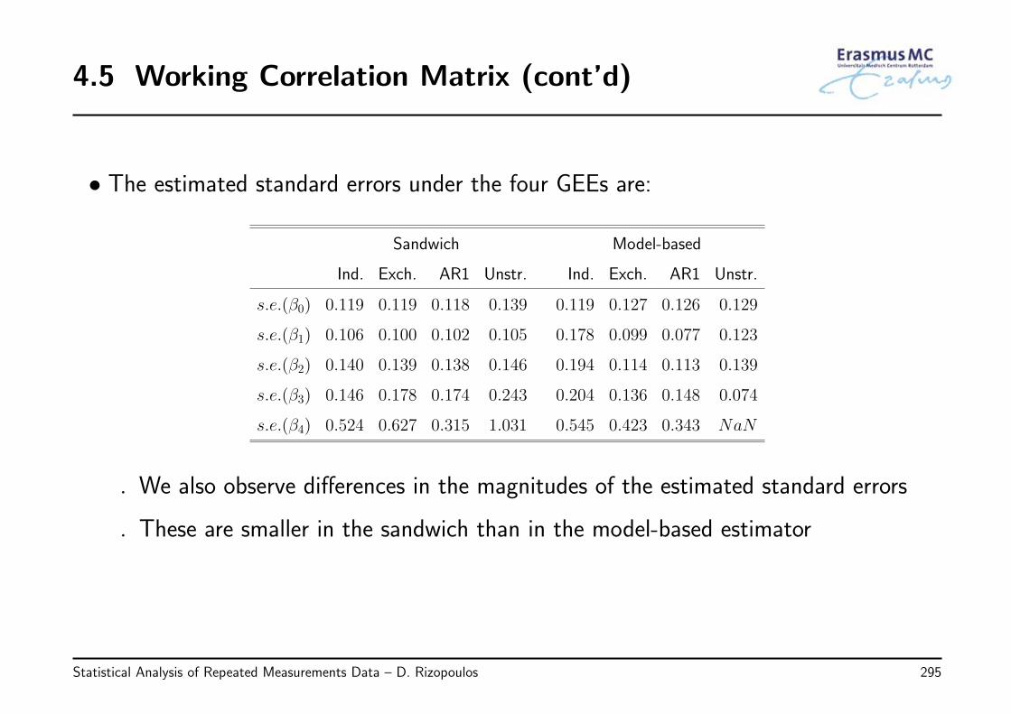
4.5 Working Correlation Matrix (cont’d)
• The estimated standard errors under the four GEEs are:
Sandwich Model-based
Ind. Exch. AR1 Unstr. Ind. Exch. AR1 Unstr.
s.e.(β0) 0.119 0.119 0.118 0.139 0.119 0.127 0.126 0.129
s.e.(β1) 0.106 0.100 0.102 0.105 0.178 0.099 0.077 0.123
s.e.(β2) 0.140 0.139 0.138 0.146 0.194 0.114 0.113 0.139
s.e.(β3) 0.146 0.178 0.174 0.243 0.204 0.136 0.148 0.074
s.e.(β4) 0.524 0.627 0.315 1.031 0.545 0.423 0.343 NaN
◃ We also observe differences in the magnitudes of the estimated standard errors
◃ These are smaller in the sandwich than in the model-based estimator
Statistical Analysis of Repeated Measurements Data – D. Rizopoulos 295
4.5 Working Correlation Matrix (cont’d)
• How to choose the most appropriate working correlation matrix?
◃ unfortunately, there are no generally accepted formal tests for choosing theworking correlation matrix
◃ the choice should not be based on the grounds of statistical significance
◃ consider appropriate choices based on the features of the data
* for balanced data with big sample size ⇒ Unstructured
* unbalanced data ⇒ Exchangeable or AR1
* when more than one options plausible ⇒ sensitivity analysis, report all results
Similarly to what we have seen in Chapter 2 and 3, a prerequisiteis that the mean structure is correctly specified
Statistical Analysis of Repeated Measurements Data – D. Rizopoulos 296
4.6 Hypothesis Testing
• Having fitted a GEE model often scientific interest lies in testing specific hypotheses
• Due to the fact that GEE models are semiparametric models, we can only employWald tests to test the hypothesis of interest
◃ score and likelihood ratio tests are not available
• In addition, in standard GEEs, these tests are only available for the mean parameters(i.e., the regression coefficients) and not the parameters of the working correlationmatrix
Statistical Analysis of Repeated Measurements Data – D. Rizopoulos 297
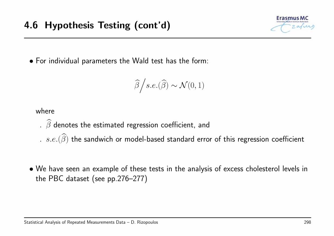
4.6 Hypothesis Testing (cont’d)
• For individual parameters the Wald test has the form:
β/s.e.(β) ∼ N (0, 1)
where
◃ β denotes the estimated regression coefficient, and
◃ s.e.(β) the sandwich or model-based standard error of this regression coefficient
• We have seen an example of these tests in the analysis of excess cholesterol levels inthe PBC dataset (see pp.276–277)
Statistical Analysis of Repeated Measurements Data – D. Rizopoulos 298
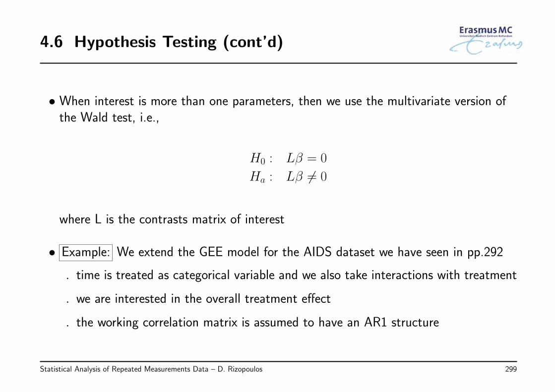
4.6 Hypothesis Testing (cont’d)
• When interest is more than one parameters, then we use the multivariate version ofthe Wald test, i.e.,
H0 : Lβ = 0
Ha : Lβ = 0
where L is the contrasts matrix of interest
• Example: We extend the GEE model for the AIDS dataset we have seen in pp.292
◃ time is treated as categorical variable and we also take interactions with treatment
◃ we are interested in the overall treatment effect
◃ the working correlation matrix is assumed to have an AR1 structure
Statistical Analysis of Repeated Measurements Data – D. Rizopoulos 299
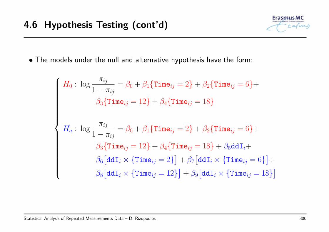
4.6 Hypothesis Testing (cont’d)
• The models under the null and alternative hypothesis have the form:
H0 : logπij
1− πij= β0 + β1{Timeij = 2} + β2{Timeij = 6}+
β3{Timeij = 12} + β4{Timeij = 18}
Ha : logπij
1− πij= β0 + β1{Timeij = 2} + β2{Timeij = 6}+
β3{Timeij = 12} + β4{Timeij = 18} + β5ddIi+
β6[ddIi × {Timeij = 2}
]+ β7
[ddIi × {Timeij = 6}
]+
β8[ddIi × {Timeij = 12}
]+ β9
[ddIi × {Timeij = 18}
]
Statistical Analysis of Repeated Measurements Data – D. Rizopoulos 300
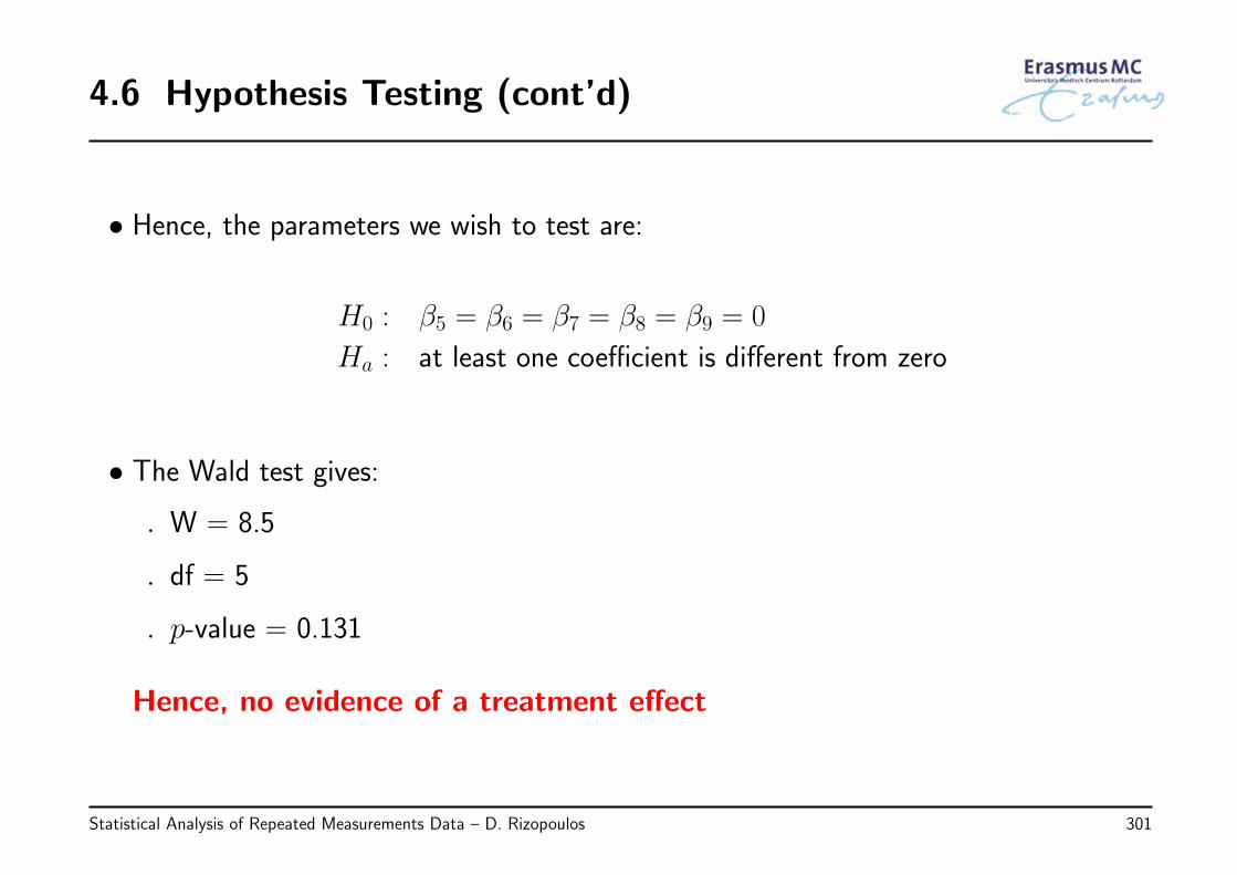
4.6 Hypothesis Testing (cont’d)
• Hence, the parameters we wish to test are:
H0 : β5 = β6 = β7 = β8 = β9 = 0
Ha : at least one coefficient is different from zero
• The Wald test gives:
◃ W = 8.5
◃ df = 5
◃ p-value = 0.131
Hence, no evidence of a treatment effect
Statistical Analysis of Repeated Measurements Data – D. Rizopoulos 301
4.6 Hypothesis Testing (cont’d)
• Note that we could also apply a multivariate test not only with a contrast matrix L,but also with a design matrix of interest X
• Example: We fit a GEE model for excess serum cholesterol levels in which we includethe following terms
◃ nonlinear effect of time with natural cubic splines with 3 degrees of freedom
◃ main effect of treatment
◃ interaction of treatment with nonlinear effect of time
◃ nonlinear effect of baseline age with natural cubic splines with 3 degrees offreedom
Statistical Analysis of Repeated Measurements Data – D. Rizopoulos 302
4.6 Hypothesis Testing (cont’d)
• As we have previously discussed, when we include nonlinear terms parameters do nothave a straightforward interpretation
• But we could still test meaningful hypothesis
◃ more specifically, we are interested in testing for a treatment effect at year 7 forpatients who are 49 years old
• Let X1 denote the design matrix of the placebo patient at year 7 and age 49, and X2
the analogous design matrix for the patient who receives D-penicillamine
Statistical Analysis of Repeated Measurements Data – D. Rizopoulos 303
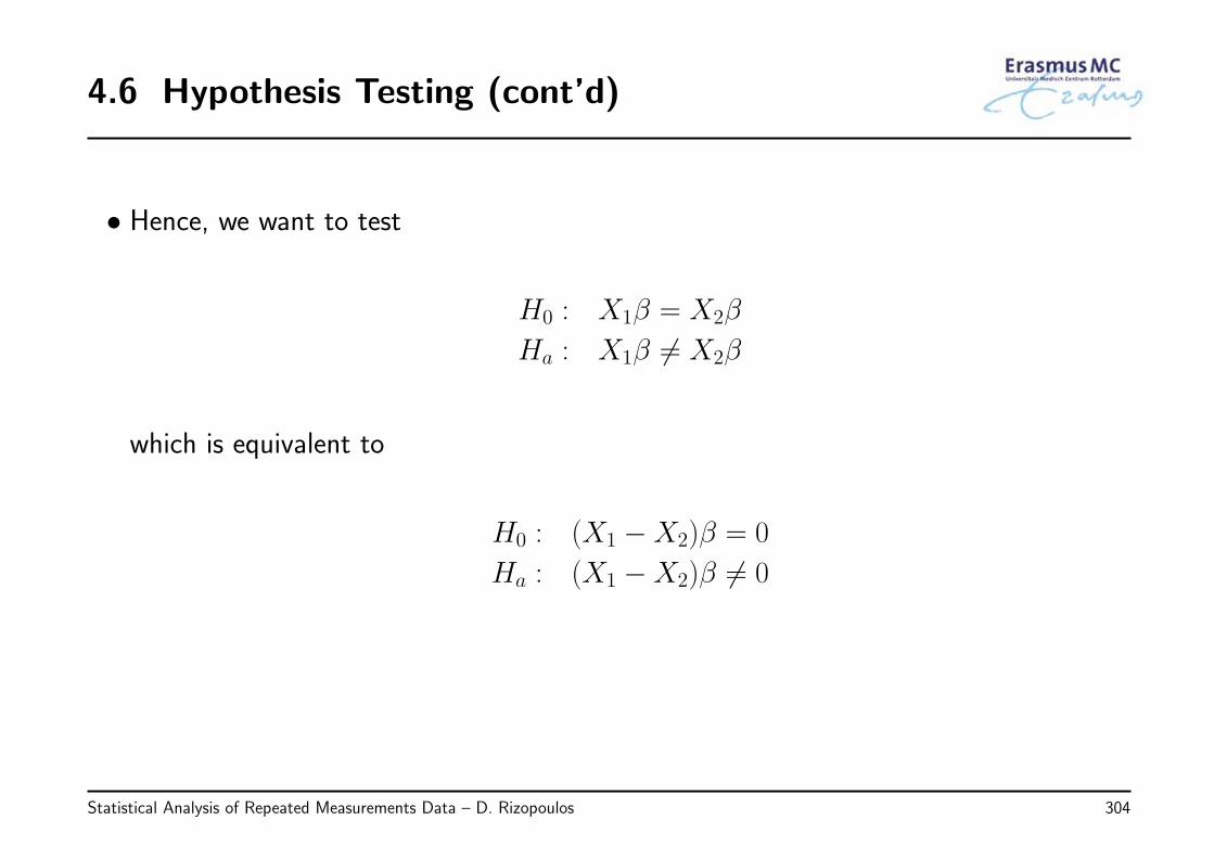
4.6 Hypothesis Testing (cont’d)
• Hence, we want to test
H0 : X1β = X2β
Ha : X1β = X2β
which is equivalent to
H0 : (X1 −X2)β = 0
Ha : (X1 −X2)β = 0
Statistical Analysis of Repeated Measurements Data – D. Rizopoulos 304
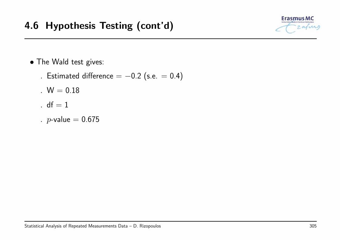
4.6 Hypothesis Testing (cont’d)
• The Wald test gives:
◃ Estimated difference = −0.2 (s.e. = 0.4)
◃ W = 0.18
◃ df = 1
◃ p-value = 0.675
Statistical Analysis of Repeated Measurements Data – D. Rizopoulos 305
4.7 Review of Key Points
• Generalized Estimating Equations: What they are
◃ extension of the marginal models we have seen in Chapter 2, in the setting ofcategorical data
◃ Three components: (i) a model for the mean, (ii) a model for the variance, &(iii) an assumption for the pairwise correlations
◃ semiparametric approach ⇒ no assumptions for the distribution of the data
• Generalized Estimating Equations: Features
◃ important to correctly specify the mean
◃ sandwich estimator protects against misspecification of the working correlationbut works (satisfactorily) under specific settings
Statistical Analysis of Repeated Measurements Data – D. Rizopoulos 306
4.7 Review of Key Points (cont’d)
• Generalized Estimating Equations: Features
◃ only Wald tests available
◃ strict assumptions with respect to incomplete data
Statistical Analysis of Repeated Measurements Data – D. Rizopoulos 307

Chapter 5
Mixed Models for Discrete Data
Statistical Analysis of Repeated Measurements Data – D. Rizopoulos 308
5.1 Generalized Linear Mixed Models
• The previous chapter focused on the framework of Generalized Estimating Equations
◃ this can be seen as the extension of the marginal models for continuous data ofChapter 2 to the setting of categorical longitudinal responses
• In this chapter we will see the analogue of linear mixed models for categorical data
⇓
Generalized Linear Mixed Models (GLMMs)
Statistical Analysis of Repeated Measurements Data – D. Rizopoulos 309
5.1 Generalized Linear Mixed Models (cont’d)
• The intuitive idea behind GLMMs is the same as in linear mixed models, i.e.,
◃ the correlation between the repeated categorical measurements is induced byunobserved random effects
◃ in other words: the categorical longitudinal measurements of a subject arecorrelated because all of them share the same unobserved random effect(conditional independence assumption)
Statistical Analysis of Repeated Measurements Data – D. Rizopoulos 310
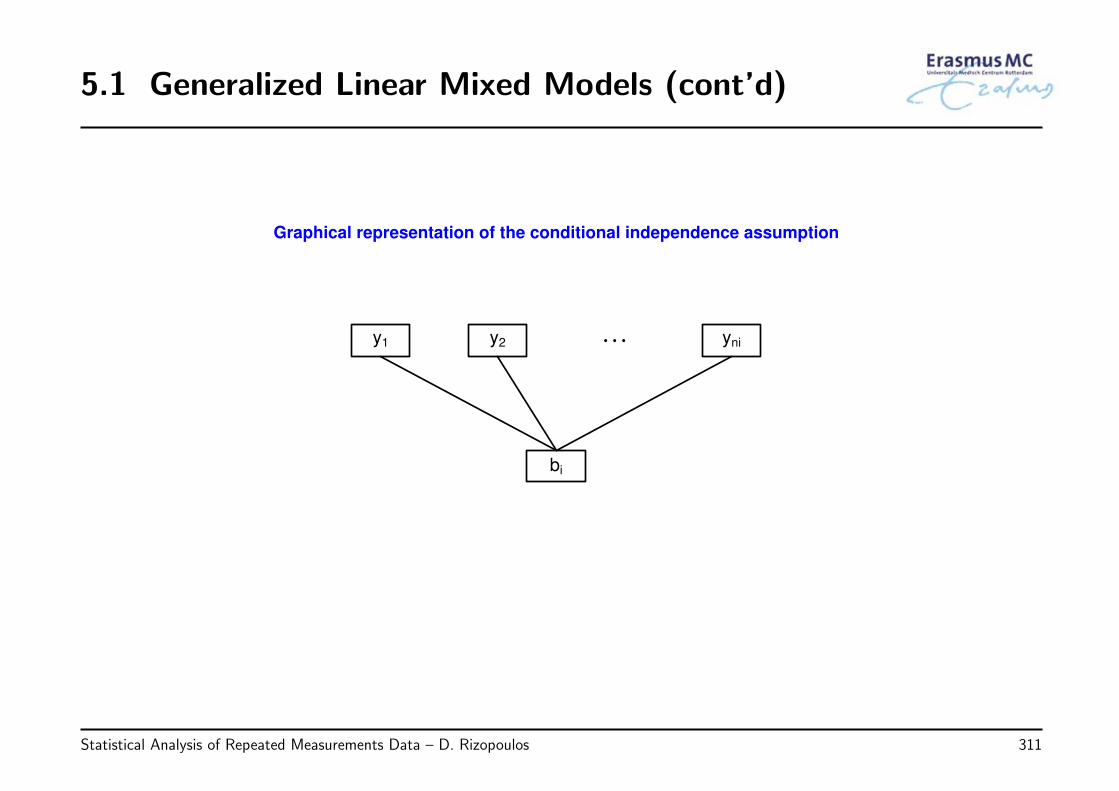
5.1 Generalized Linear Mixed Models (cont’d)
Graphical representation of the conditional independence assumption
y1 y2 yni
bi
…
Statistical Analysis of Repeated Measurements Data – D. Rizopoulos 311
5.1 Generalized Linear Mixed Models (cont’d)
• Similarly to Chapter 4, we will focus on clustered dichotomous/binary data
◃ nonetheless, the same ideas and issues also apply to other categorical responses(e.g., Poisson, ordinal data, multinomial data, etc.)
• Suppose we have a binary outcome yij
yij =
1, if subject i has a positive response at measurement j
0, if subject i has a negative response at measurement j
Statistical Analysis of Repeated Measurements Data – D. Rizopoulos 312
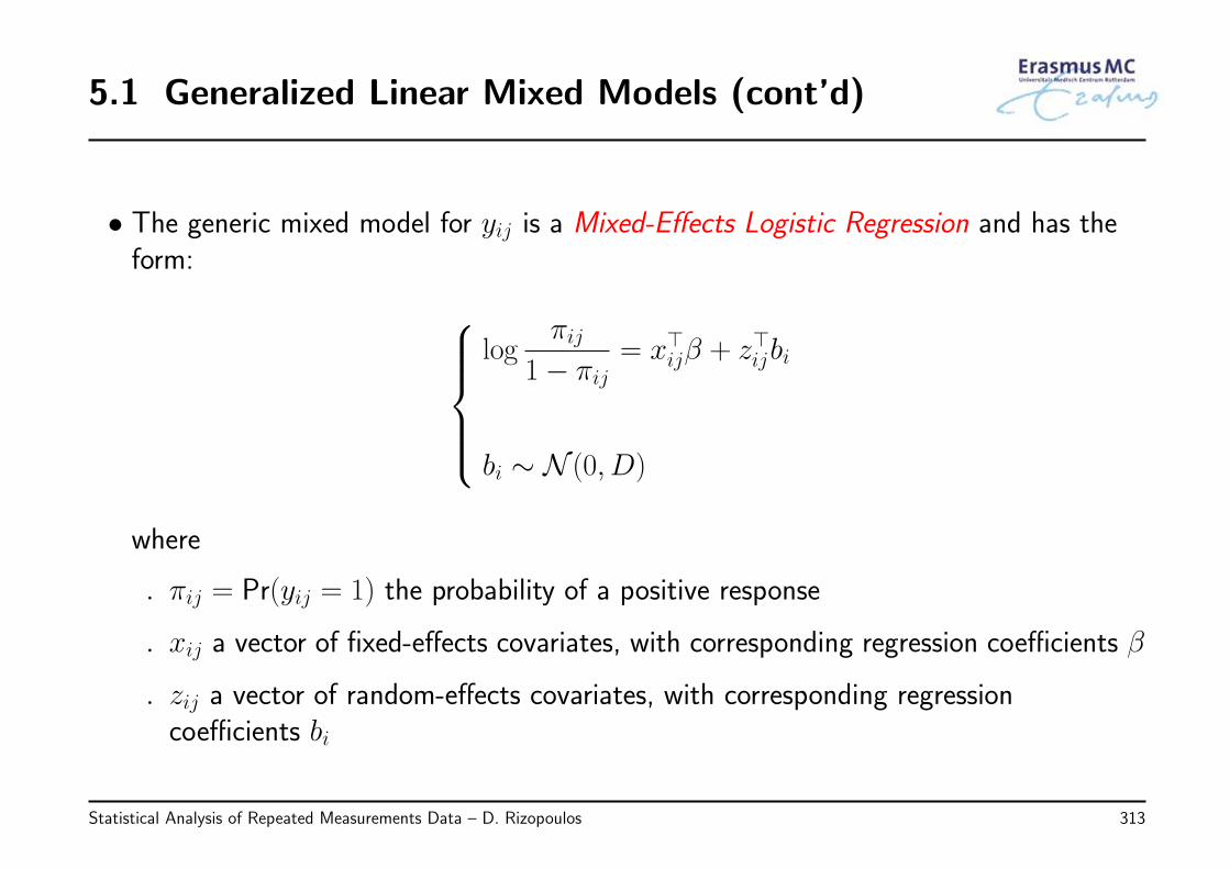
5.1 Generalized Linear Mixed Models (cont’d)
• The generic mixed model for yij is a Mixed-Effects Logistic Regression and has theform:
log
πij1− πij
= x⊤ijβ + z⊤ijbi
bi ∼ N (0, D)
where
◃ πij = Pr(yij = 1) the probability of a positive response
◃ xij a vector of fixed-effects covariates, with corresponding regression coefficients β
◃ zij a vector of random-effects covariates, with corresponding regressioncoefficients bi
Statistical Analysis of Repeated Measurements Data – D. Rizopoulos 313
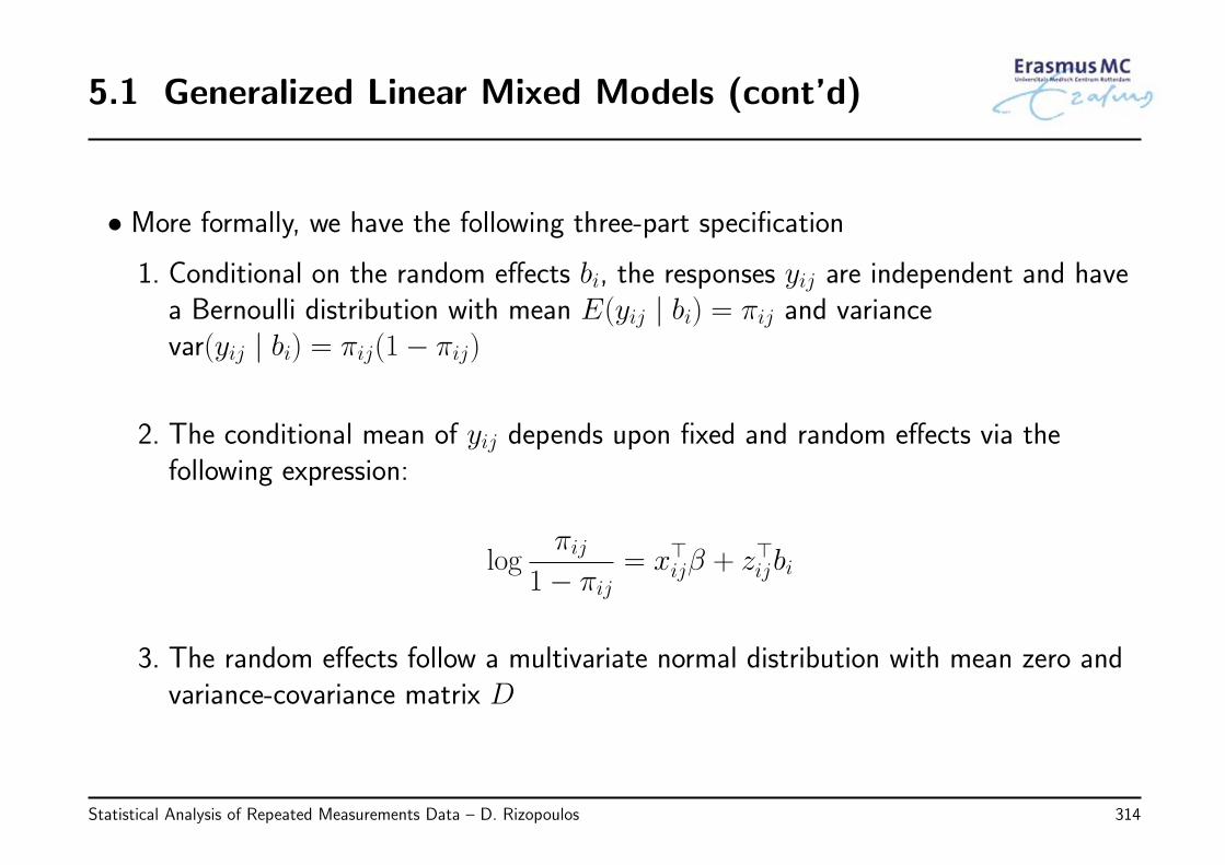
5.1 Generalized Linear Mixed Models (cont’d)
• More formally, we have the following three-part specification
1. Conditional on the random effects bi, the responses yij are independent and havea Bernoulli distribution with mean E(yij | bi) = πij and variancevar(yij | bi) = πij(1− πij)
2. The conditional mean of yij depends upon fixed and random effects via thefollowing expression:
logπij
1− πij= x⊤ijβ + z⊤ijbi
3. The random effects follow a multivariate normal distribution with mean zero andvariance-covariance matrix D
Statistical Analysis of Repeated Measurements Data – D. Rizopoulos 314
5.1 Generalized Linear Mixed Models (cont’d)
• Notes: On the definition of GLMMs
◃ The three-part specification of GLMMs corresponds to a full specification of thedistribution of the outcome yij – this is in contrast to the GEE approach, which isa semi-parametric method
◃ The mean and correlation structures are simultaneously defined using randomeffects⇒ As we will see next, this has direct and important implications with respect tothe interpretation of the parameters
Statistical Analysis of Repeated Measurements Data – D. Rizopoulos 315
5.2 Interpretation
• Example: In the AIDS dataset, a very low CD4 count (less than 150 cells/mm3) is anindicator for opportunistic infections
◃ In the following analysis we dichotomize the CD4 cell counts from the AIDSdataset using this threshold
◃ We fit a mixed effects logistic regression with
* fixed effects: time, treatment and their interaction
* random effects: random intercepts
Statistical Analysis of Repeated Measurements Data – D. Rizopoulos 316
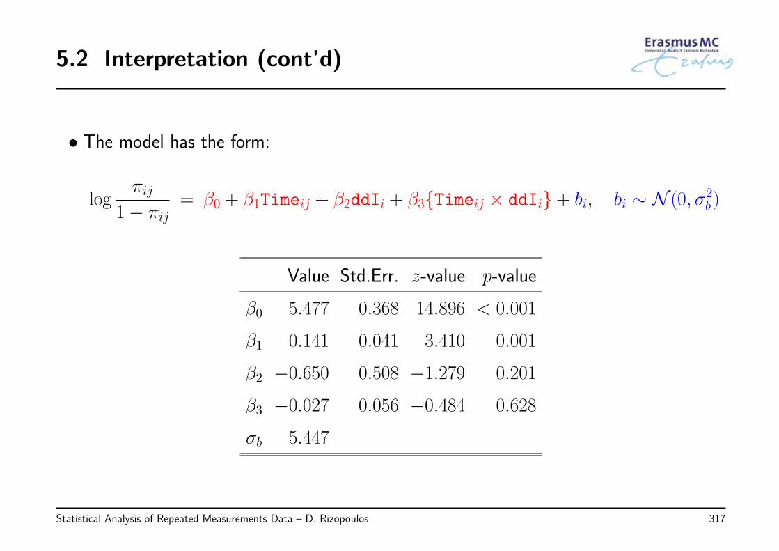
5.2 Interpretation (cont’d)
• The model has the form:
logπij
1− πij= β0 + β1Timeij + β2ddIi + β3{Timeij × ddIi} + bi, bi ∼ N (0, σ2
b )
Value Std.Err. z-value p-value
β0 5.477 0.368 14.896 < 0.001
β1 0.141 0.041 3.410 0.001
β2 −0.650 0.508 −1.279 0.201
β3 −0.027 0.056 −0.484 0.628
σb 5.447
Statistical Analysis of Repeated Measurements Data – D. Rizopoulos 317
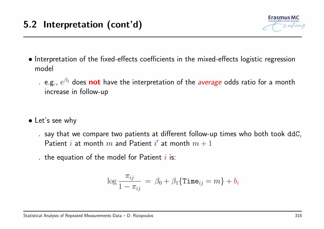
5.2 Interpretation (cont’d)
• Interpretation of the fixed-effects coefficients in the mixed-effects logistic regressionmodel
◃ e.g., eβ1 does not have the interpretation of the average odds ratio for a monthincrease in follow-up
• Let’s see why
◃ say that we compare two patients at different follow-up times who both took ddC,Patient i at month m and Patient i′ at month m + 1
◃ the equation of the model for Patient i is:
logπij
1− πij= β0 + β1{Timeij = m} + bi
Statistical Analysis of Repeated Measurements Data – D. Rizopoulos 318
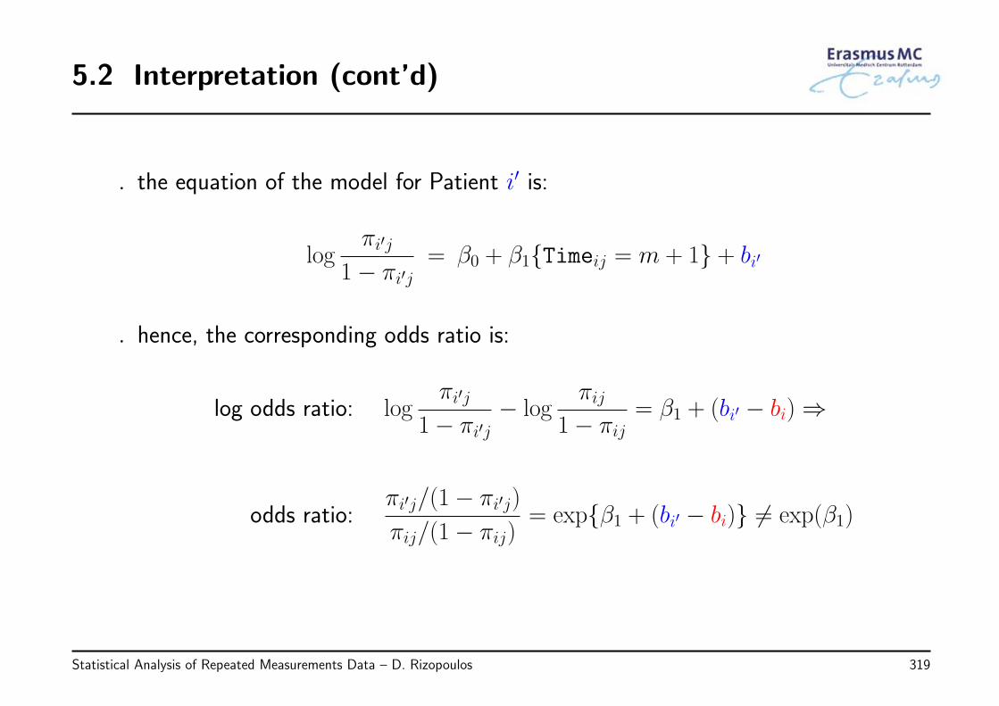
5.2 Interpretation (cont’d)
◃ the equation of the model for Patient i′ is:
logπi′j
1− πi′j= β0 + β1{Timeij = m + 1} + bi′
◃ hence, the corresponding odds ratio is:
log odds ratio: logπi′j
1− πi′j− log
πij1− πij
= β1 + (bi′ − bi) ⇒
odds ratio:πi′j/(1− πi′j)
πij/(1− πij)= exp{β1 + (bi′ − bi)} = exp(β1)
Statistical Analysis of Repeated Measurements Data – D. Rizopoulos 319
5.2 Interpretation (cont’d)
• Hence, the interpretation of eβ1 is not the odds ratio for unit increase of Timeaveraged over subjects, but rather for subjects with the same random-effect value
• To illustrate this graphically, we depict the relationship between time and theprobability of low CD4 cell counts. . .
Statistical Analysis of Repeated Measurements Data – D. Rizopoulos 320
5.2 Interpretation (cont’d)
0 2 4 6 8
0.0
0.2
0.4
0.6
0.8
1.0
Time
Pro
ba
bili
ty
Statistical Analysis of Repeated Measurements Data – D. Rizopoulos 321
5.2 Interpretation (cont’d)
◃ the grey lines depict 13 random subjects with increasing random effects
◃ the black line corresponds to the subject with bi = 0 (i.e., the mean individual)⇒ This line is actually 1/[1 + exp{−(β0 + β1Timeij)}]
◃ the red line that crosses the 13 lines denotes the average longitudinal evolution ofthe probability of low CD4 cells counts across subjects
Statistical Analysis of Repeated Measurements Data – D. Rizopoulos 322
5.2 Interpretation (cont’d)
Why is this happening? . . .
to connect the probabilities with covariates we need the non-linear logit function
Statistical Analysis of Repeated Measurements Data – D. Rizopoulos 323
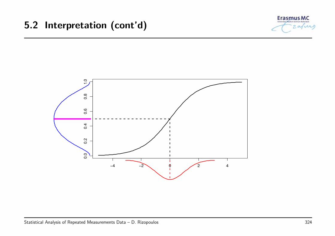
5.2 Interpretation (cont’d)
−4 −2 0 2 4
0.0
0.2
0.4
0.6
0.8
1.0
Statistical Analysis of Repeated Measurements Data – D. Rizopoulos 324
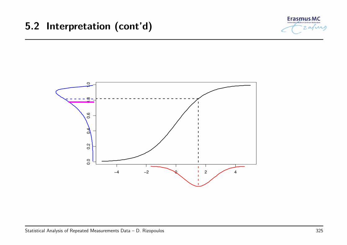
5.2 Interpretation (cont’d)
−4 −2 0 2 4
0.0
0.2
0.4
0.6
0.8
1.0
Statistical Analysis of Repeated Measurements Data – D. Rizopoulos 325
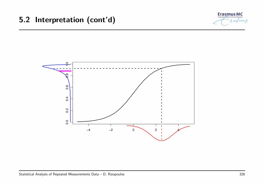
5.2 Interpretation (cont’d)
−4 −2 0 2 4
0.0
0.2
0.4
0.6
0.8
1.0
Statistical Analysis of Repeated Measurements Data – D. Rizopoulos 326
5.2 Interpretation (cont’d)
• We did not have this problem in the case of the linear mixed model because we didnot have a link function
◃ or to put it more precisely, the link function was the identity g(x) = x
• Let’s see graphically again why for linear mixed models we do not have the sameproblem . . .
Statistical Analysis of Repeated Measurements Data – D. Rizopoulos 327
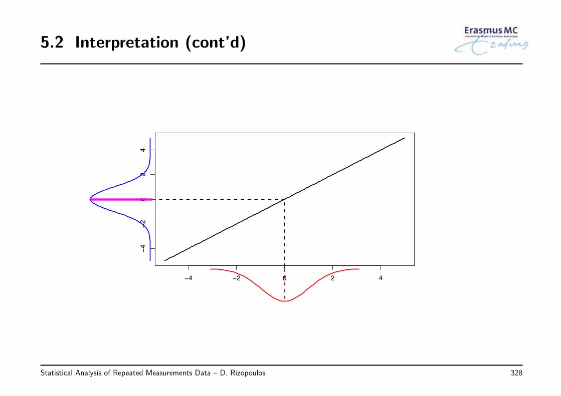
5.2 Interpretation (cont’d)
−4 −2 0 2 4
−4
−2
02
4
Statistical Analysis of Repeated Measurements Data – D. Rizopoulos 328
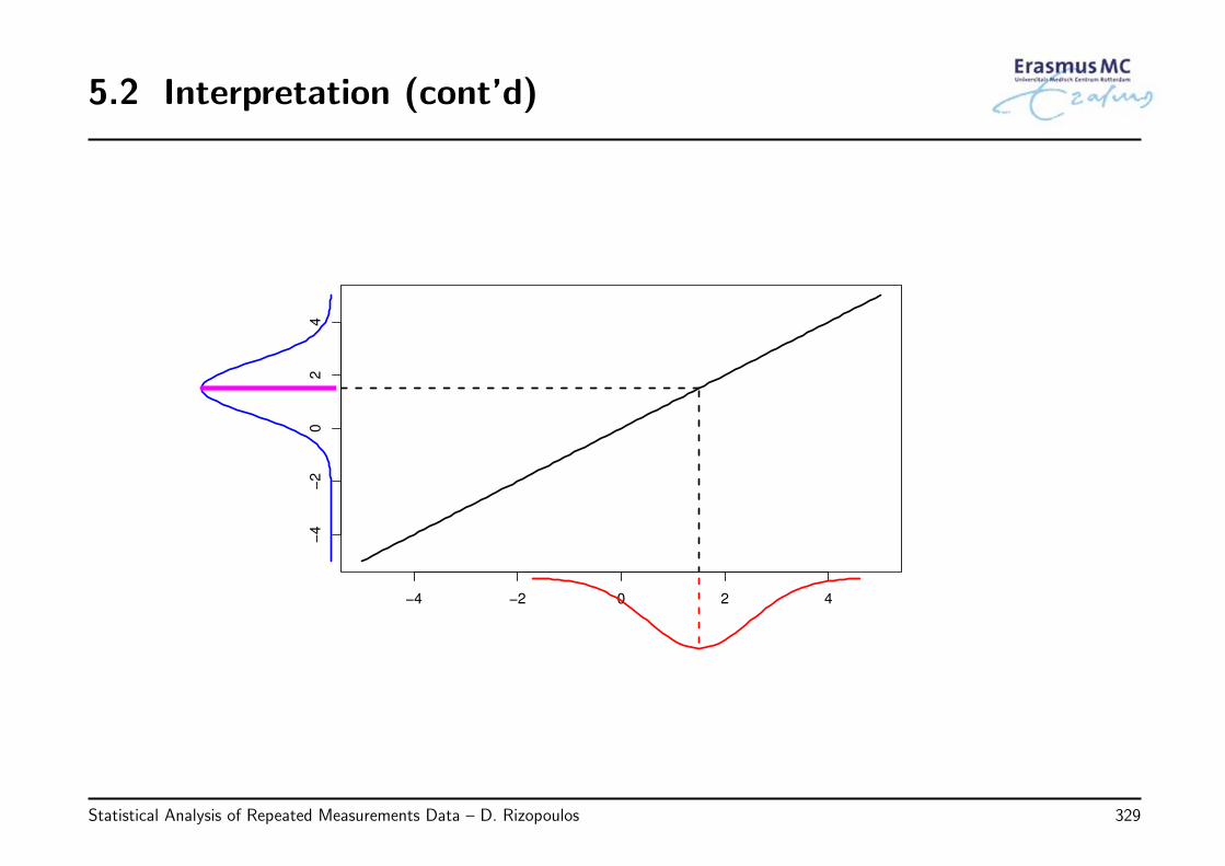
5.2 Interpretation (cont’d)
−4 −2 0 2 4
−4
−2
02
4
Statistical Analysis of Repeated Measurements Data – D. Rizopoulos 329
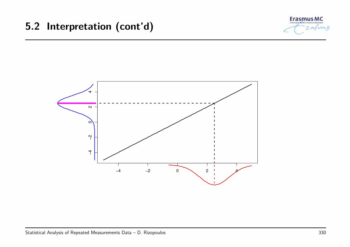
5.2 Interpretation (cont’d)
−4 −2 0 2 4
−4
−2
02
4
Statistical Analysis of Repeated Measurements Data – D. Rizopoulos 330
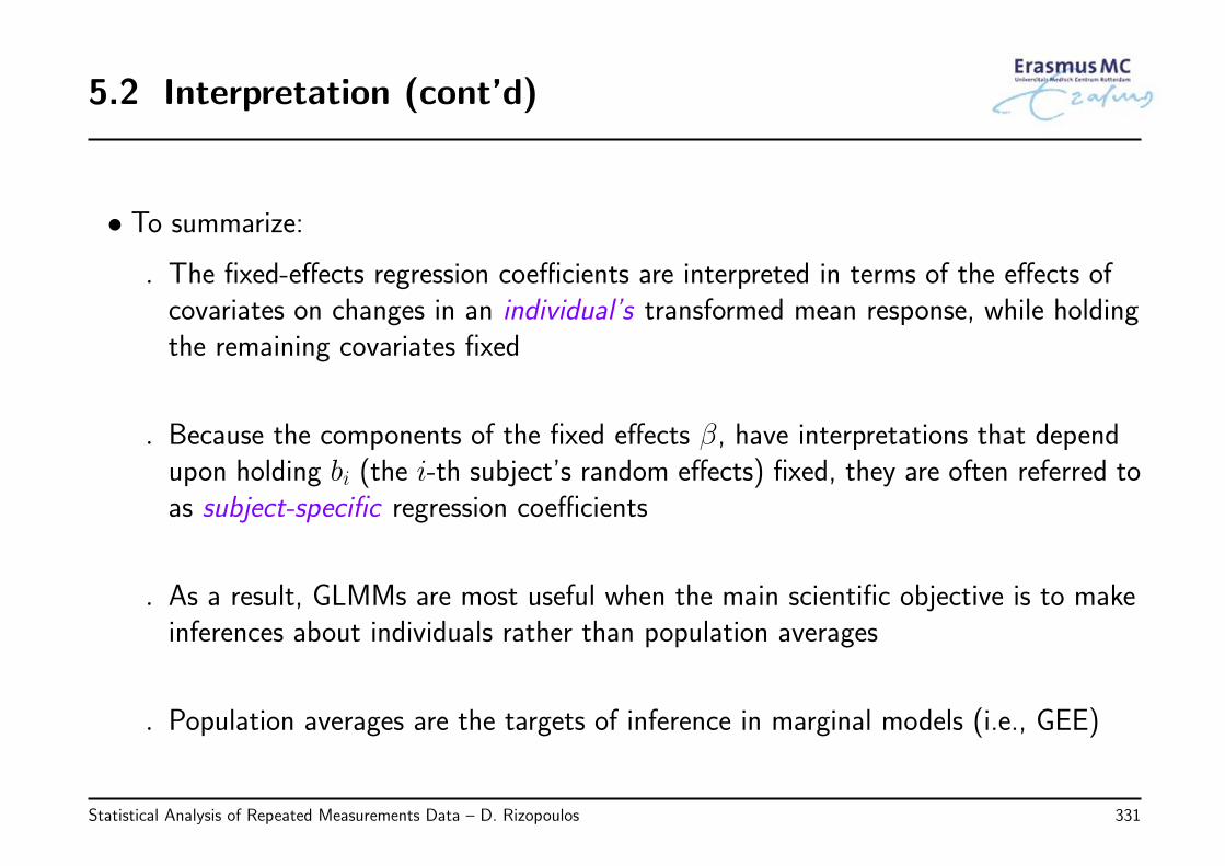
5.2 Interpretation (cont’d)
• To summarize:
◃ The fixed-effects regression coefficients are interpreted in terms of the effects ofcovariates on changes in an individual’s transformed mean response, while holdingthe remaining covariates fixed
◃ Because the components of the fixed effects β, have interpretations that dependupon holding bi (the i-th subject’s random effects) fixed, they are often referred toas subject-specific regression coefficients
◃ As a result, GLMMs are most useful when the main scientific objective is to makeinferences about individuals rather than population averages
◃ Population averages are the targets of inference in marginal models (i.e., GEE)
Statistical Analysis of Repeated Measurements Data – D. Rizopoulos 331
5.2 Interpretation (cont’d)
Hence, contrary to the marginal and mixed effects model for continuous data(Chapters 2 & 3), the regression coefficients from marginal models for discretedata do not have the same interpretation as the corresponding coefficients
from mixed effects models
Statistical Analysis of Repeated Measurements Data – D. Rizopoulos 332
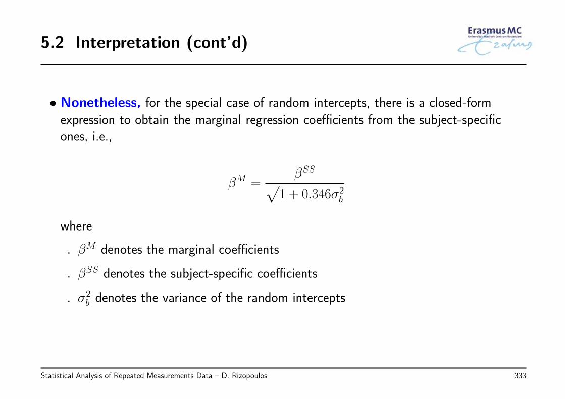
5.2 Interpretation (cont’d)
• Nonetheless, for the special case of random intercepts, there is a closed-formexpression to obtain the marginal regression coefficients from the subject-specificones, i.e.,
βM =βSS√
1 + 0.346σ2b
where
◃ βM denotes the marginal coefficients
◃ βSS denotes the subject-specific coefficients
◃ σ2b denotes the variance of the random intercepts
Statistical Analysis of Repeated Measurements Data – D. Rizopoulos 333
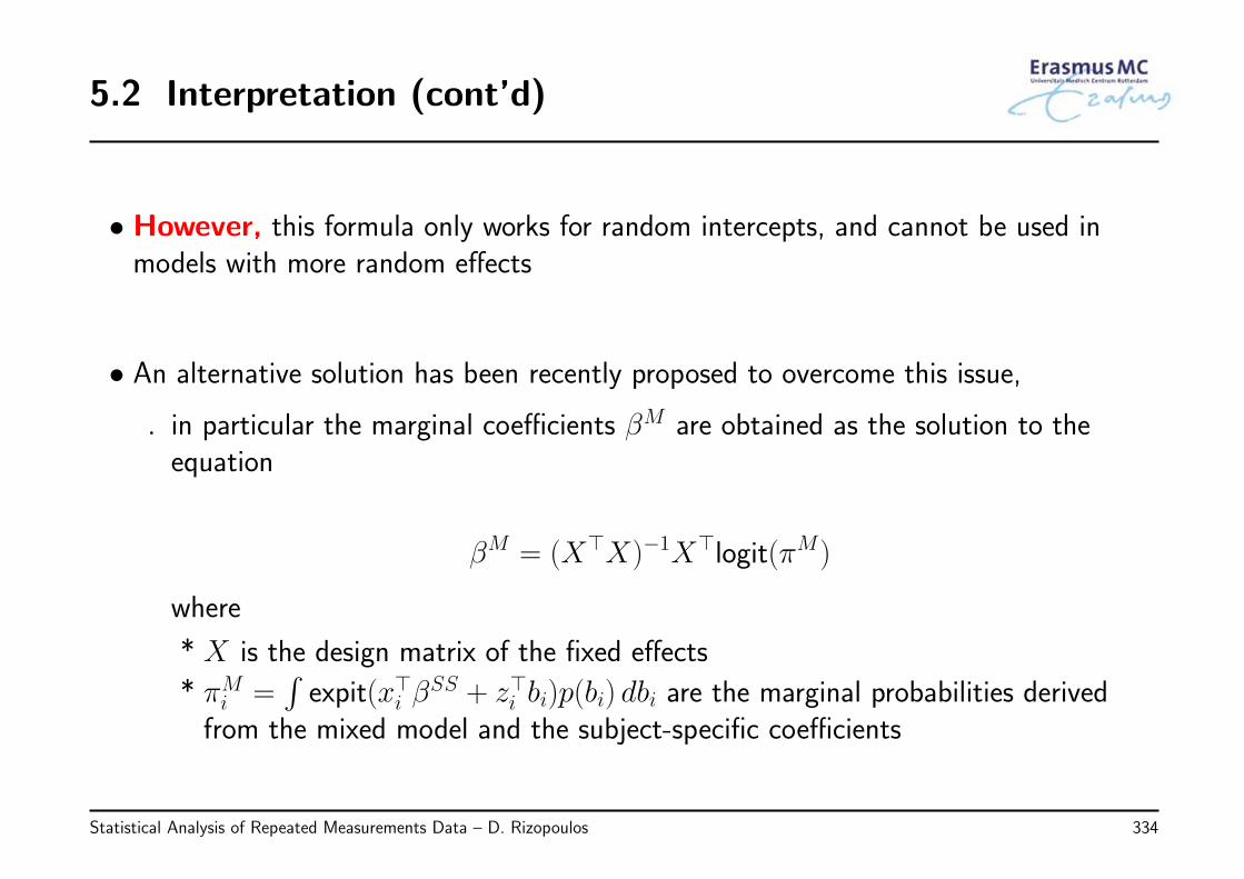
5.2 Interpretation (cont’d)
• However, this formula only works for random intercepts, and cannot be used inmodels with more random effects
• An alternative solution has been recently proposed to overcome this issue,
◃ in particular the marginal coefficients βM are obtained as the solution to theequation
βM = (X⊤X)−1X⊤logit(πM)
where
* X is the design matrix of the fixed effects
* πMi =
∫expit(x⊤i β
SS + z⊤i bi)p(bi) dbi are the marginal probabilities derivedfrom the mixed model and the subject-specific coefficients
Statistical Analysis of Repeated Measurements Data – D. Rizopoulos 334
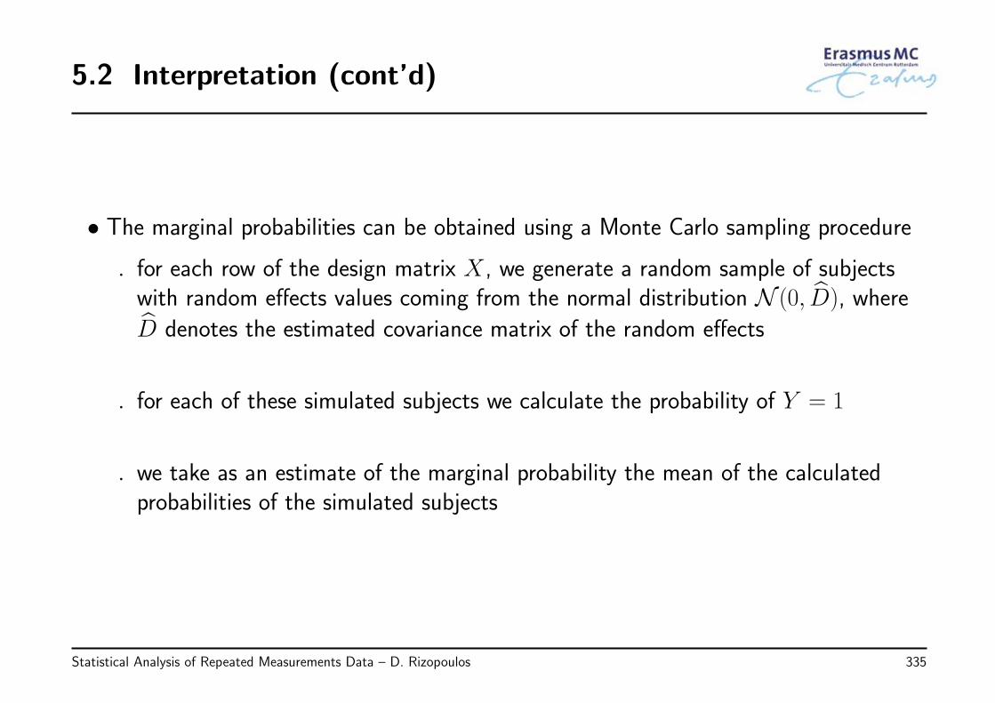
5.2 Interpretation (cont’d)
• The marginal probabilities can be obtained using a Monte Carlo sampling procedure
◃ for each row of the design matrix X , we generate a random sample of subjectswith random effects values coming from the normal distribution N (0, D), where
D denotes the estimated covariance matrix of the random effects
◃ for each of these simulated subjects we calculate the probability of Y = 1
◃ we take as an estimate of the marginal probability the mean of the calculatedprobabilities of the simulated subjects
Statistical Analysis of Repeated Measurements Data – D. Rizopoulos 335
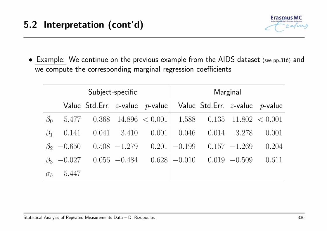
5.2 Interpretation (cont’d)
• Example: We continue on the previous example from the AIDS dataset (see pp.316) andwe compute the corresponding marginal regression coefficients
Subject-specific Marginal
Value Std.Err. z-value p-value Value Std.Err. z-value p-value
β0 5.477 0.368 14.896 < 0.001 1.588 0.135 11.802 < 0.001
β1 0.141 0.041 3.410 0.001 0.046 0.014 3.278 0.001
β2 −0.650 0.508 −1.279 0.201 −0.199 0.157 −1.269 0.204
β3 −0.027 0.056 −0.484 0.628 −0.010 0.019 −0.509 0.611
σb 5.447
Statistical Analysis of Repeated Measurements Data – D. Rizopoulos 336
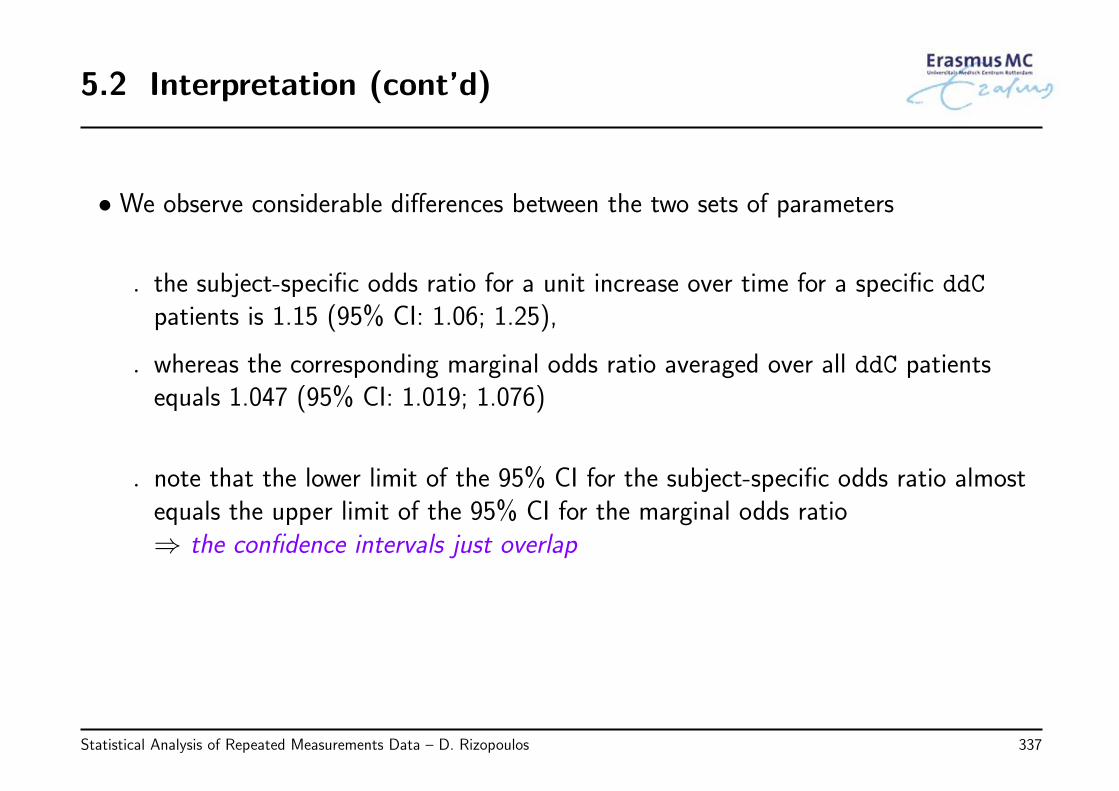
5.2 Interpretation (cont’d)
• We observe considerable differences between the two sets of parameters
◃ the subject-specific odds ratio for a unit increase over time for a specific ddCpatients is 1.15 (95% CI: 1.06; 1.25),
◃ whereas the corresponding marginal odds ratio averaged over all ddC patientsequals 1.047 (95% CI: 1.019; 1.076)
◃ note that the lower limit of the 95% CI for the subject-specific odds ratio almostequals the upper limit of the 95% CI for the marginal odds ratio⇒ the confidence intervals just overlap
Statistical Analysis of Repeated Measurements Data – D. Rizopoulos 337
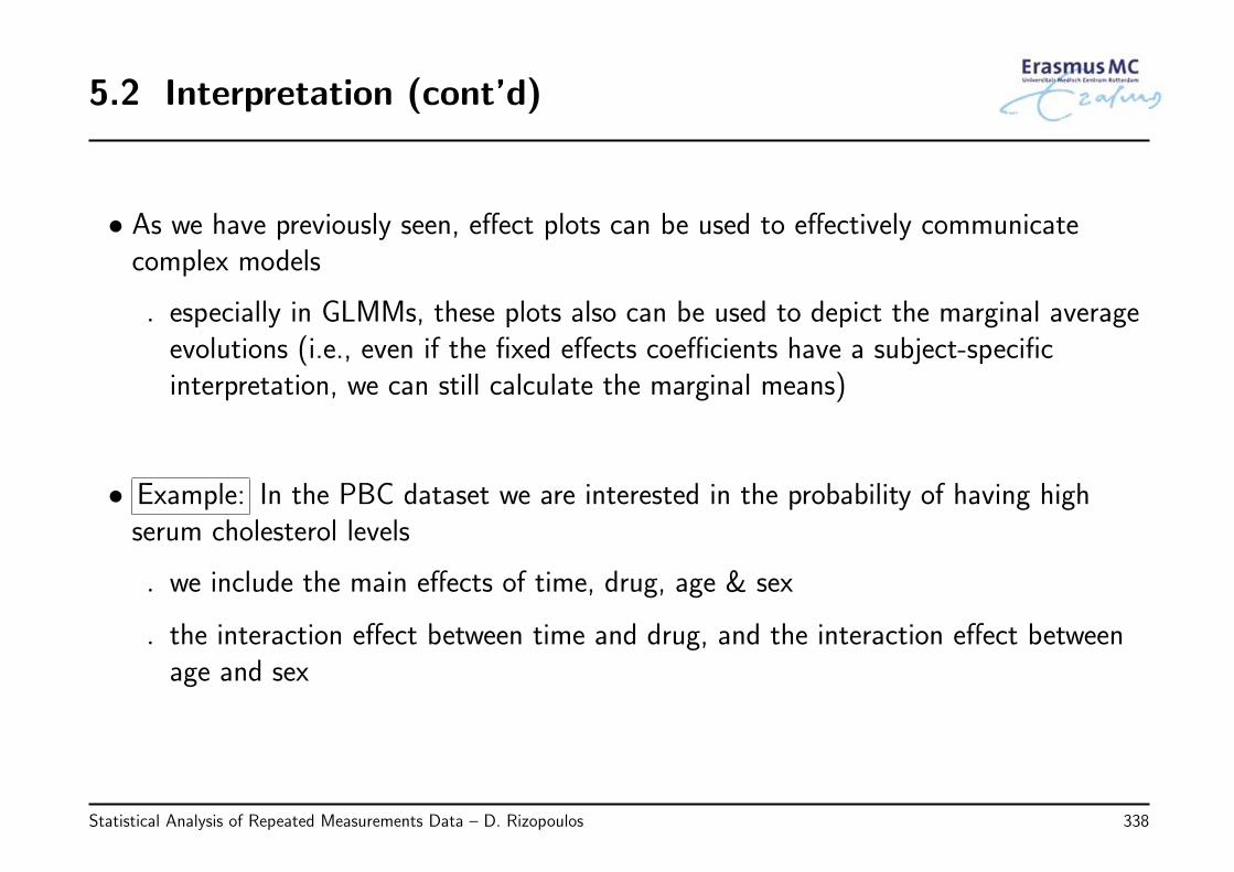
5.2 Interpretation (cont’d)
• As we have previously seen, effect plots can be used to effectively communicatecomplex models
◃ especially in GLMMs, these plots also can be used to depict the marginal averageevolutions (i.e., even if the fixed effects coefficients have a subject-specificinterpretation, we can still calculate the marginal means)
• Example: In the PBC dataset we are interested in the probability of having highserum cholesterol levels
◃ we include the main effects of time, drug, age & sex
◃ the interaction effect between time and drug, and the interaction effect betweenage and sex
Statistical Analysis of Repeated Measurements Data – D. Rizopoulos 338
5.2 Interpretation (cont’d)
• In the following figure we depict the log odds ratio as a function of time, separatelyfor each combination of the randomized treatment and sex, for the average/medianpatient
◃ average/median patient is the one with random effects values equal to zero
Statistical Analysis of Repeated Measurements Data – D. Rizopoulos 339
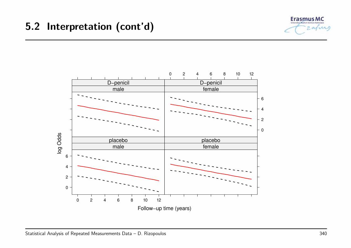
5.2 Interpretation (cont’d)
Follow−up time (years)
log
Odd
s
0
2
4
6
0 2 4 6 8 10 12
male
placebo
female
placebo
male
D−penicil
0 2 4 6 8 10 12
0
2
4
6
female
D−penicil
Statistical Analysis of Repeated Measurements Data – D. Rizopoulos 340

5.2 Interpretation (cont’d)
• In the following figure we depict the marginal probabilities, as a function for time,separately for each combination of randomized treatment and sex
◃ contrary to the previous figure, these probabilities are averaged over the patients
◃ they are obtained using the marginalized coefficients, presented in pp.334
◃ to see the difference, the blue line corresponds to the probabilities of the averagepatient
Statistical Analysis of Repeated Measurements Data – D. Rizopoulos 341
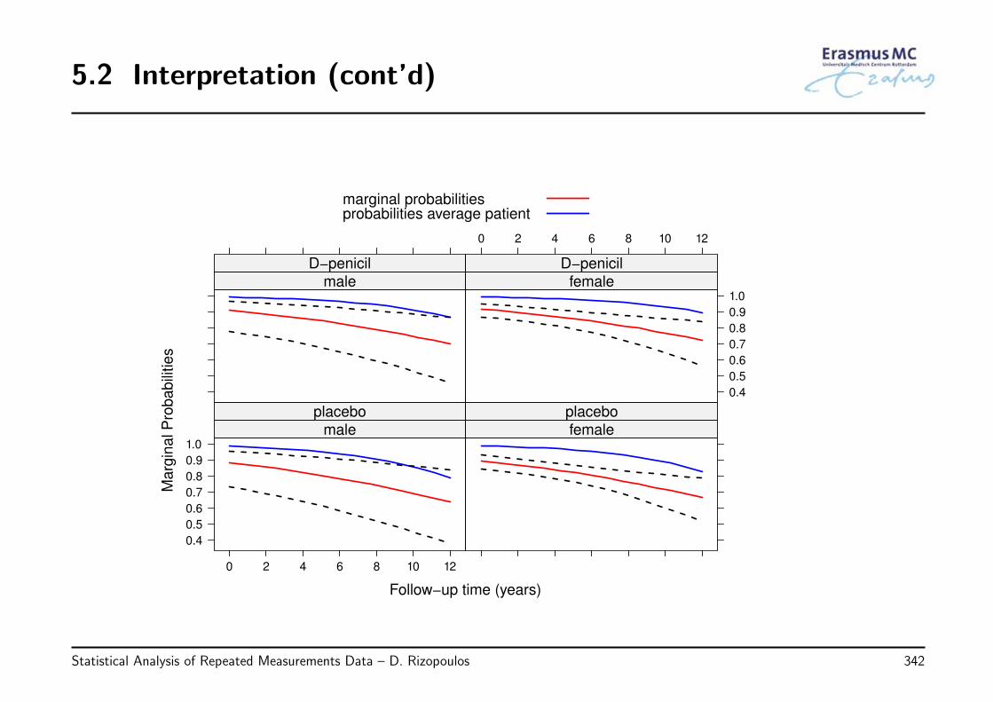
5.2 Interpretation (cont’d)
Follow−up time (years)
Ma
rgin
al P
rob
ab
ilitie
s
0.4
0.5
0.6
0.7
0.8
0.9
1.0
0 2 4 6 8 10 12
male
placebo
female
placebo
male
D−penicil
0 2 4 6 8 10 12
0.4
0.5
0.6
0.7
0.8
0.9
1.0female
D−penicil
marginal probabilitiesprobabilities average patient
Statistical Analysis of Repeated Measurements Data – D. Rizopoulos 342
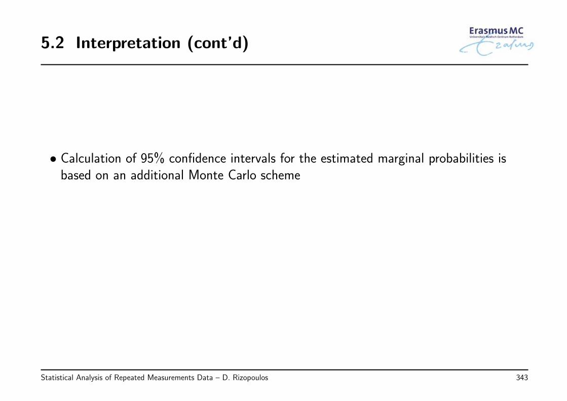
5.2 Interpretation (cont’d)
• Calculation of 95% confidence intervals for the estimated marginal probabilities isbased on an additional Monte Carlo scheme
Statistical Analysis of Repeated Measurements Data – D. Rizopoulos 343
5.3 Estimation
• The estimation of GLMMs is based on the same principles as in marginal and mixedmodels for continuous data
◃ i.e., we have a full specification of the distribution of the data (contrary to GEE),and hence we can use maximum likelihood
• Nevertheless, there is an important complication in GLMMs
The fitting of GLMMs is a computationally challenging task!
Statistical Analysis of Repeated Measurements Data – D. Rizopoulos 344
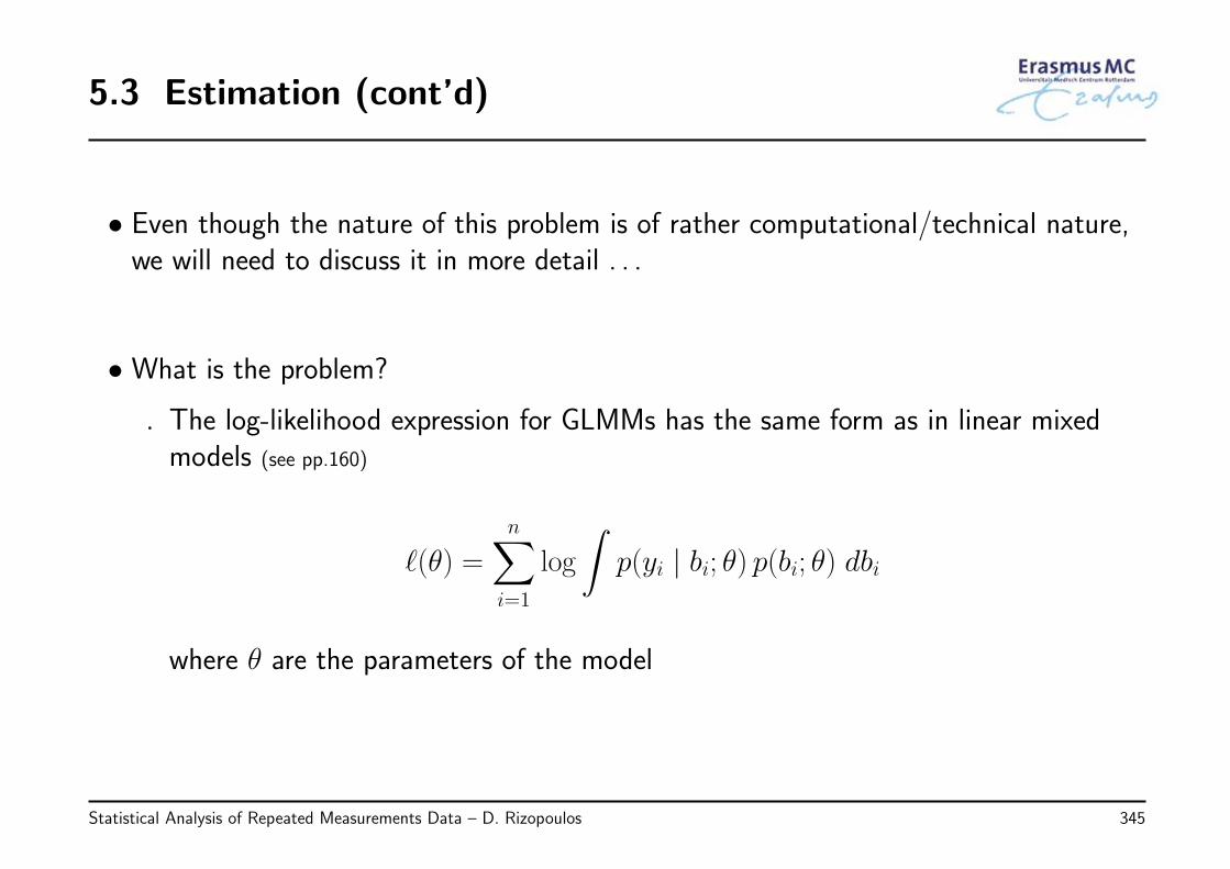
5.3 Estimation (cont’d)
• Even though the nature of this problem is of rather computational/technical nature,we will need to discuss it in more detail . . .
• What is the problem?
◃ The log-likelihood expression for GLMMs has the same form as in linear mixedmodels (see pp.160)
ℓ(θ) =
n∑i=1
log
∫p(yi | bi; θ) p(bi; θ) dbi
where θ are the parameters of the model
Statistical Analysis of Repeated Measurements Data – D. Rizopoulos 345
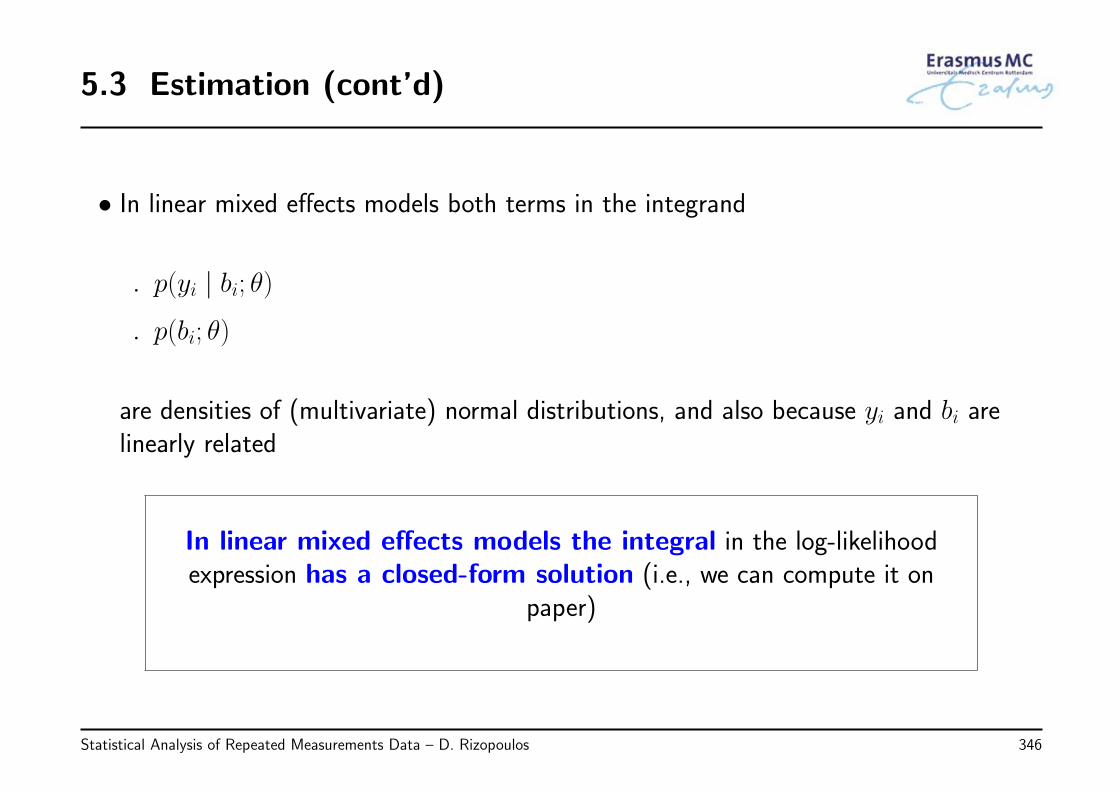
5.3 Estimation (cont’d)
• In linear mixed effects models both terms in the integrand
◃ p(yi | bi; θ)
◃ p(bi; θ)
are densities of (multivariate) normal distributions, and also because yi and bi arelinearly related
In linear mixed effects models the integral in the log-likelihoodexpression has a closed-form solution (i.e., we can compute it on
paper)
Statistical Analysis of Repeated Measurements Data – D. Rizopoulos 346
5.3 Estimation (cont’d)
• In GLMMs the two terms of the integrand denote densities of different distributions –e.g., in mixed effects logistic regression
◃ p(yi | bi; θ) ⇒ Bernoulli distribution
◃ p(bi; θ) ⇒ multivariate normal distribution
The implication is that
In GLMMs the same integral does not have a closed-formsolution
Statistical Analysis of Repeated Measurements Data – D. Rizopoulos 347
5.3 Estimation (cont’d)
• To overcome this problem two general types of solutions have been proposed in theliterature
◃ Approximation of the integrand: this entails approximating the product inside theintegral (i.e., {p(yi | bi; θ)p(yi | bi; θ)}) by a multivariate normal distribution forwhich the integral has a closed-form solution
* Penalized Quasi Likelihood (PQL)
* Laplace approximation
◃ Approximation of the integral: this entails approximating the whole integral (i.e.,∫p(yi | bi; θ)p(yi | bi; θ)dbi) by a sum
* Gaussian Quadrature & adaptive Gaussian Quadrature
* Monte Carlo & MCMC (Bayesian approach)
Statistical Analysis of Repeated Measurements Data – D. Rizopoulos 348
5.3 Estimation (cont’d)
From the two alternatives, methods that rely onapproximation of the integral have been shown to be superior
• Though they are (much) more computationally demanding – they have a parameterthat controls the accuracy of the approximation:
◃ in Gaussian quadrature rules it is the number of quadrature points (adaptiveGaussian quadrature with 1 point is equivalent to the Laplace approximation)
◃ in Monte Carlo/MCMC approaches it is the number of samples
Statistical Analysis of Repeated Measurements Data – D. Rizopoulos 349
5.3 Estimation (cont’d)
• Example: We continue on the AIDS example, but we now treat the time variable asa factor (i.e., categorical) – the model has the form:
logπij
1− πij= β0 + β1{Timeij = 2} + β2{Timeij = 6} + β3{Timeij = 12} +
β4{Timeij = 18} + bi
where
◃ πij = Pr(CD4ij < 150)
◃ {Timeij = 2} denotes the dummy variable for month 2, {Timeij = 6} the dummyvariable for month 6, and so on
Statistical Analysis of Repeated Measurements Data – D. Rizopoulos 350
5.3 Estimation (cont’d)
• We have fitted this model using
◃ PQL
◃ Laplace approximation (adaptive Gaussian quadrature with 1 point)
◃ adaptive Gaussian quadrature with 7, 10, 15 and 21 points
• The following figure depicts the estimated fixed effect coefficients under eachapproximation with corresponding 95% CIs
Statistical Analysis of Repeated Measurements Data – D. Rizopoulos 351
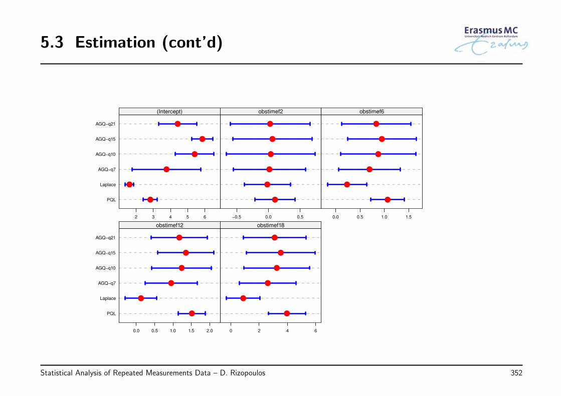
5.3 Estimation (cont’d)
PQL
Laplace
AGQ−q7
AGQ−q10
AGQ−q15
AGQ−q21
2 3 4 5 6
(Intercept)
−0.5 0.0 0.5
obstimef2
0.0 0.5 1.0 1.5
obstimef6
PQL
Laplace
AGQ−q7
AGQ−q10
AGQ−q15
AGQ−q21
0.0 0.5 1.0 1.5 2.0
obstimef12
0 2 4 6
obstimef18
Statistical Analysis of Repeated Measurements Data – D. Rizopoulos 352
5.3 Estimation (cont’d)
• We observe considerable differences between
◃ PQL & Laplace (approximation of the integrand), and
◃ adaptive Gaussian quadrature (approximation of the integral)
• In general, PQL and Laplace will work better as the data get more ‘continuous’, i.e.,
◃ in Bernoulli data as the number of repeated measurements increases considerably
◃ in Binomial data as the number of trials increases
◃ in Poisson data as the rate increases
Statistical Analysis of Repeated Measurements Data – D. Rizopoulos 353
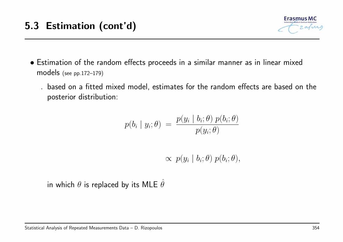
5.3 Estimation (cont’d)
• Estimation of the random effects proceeds in a similar manner as in linear mixedmodels (see pp.172–179)
◃ based on a fitted mixed model, estimates for the random effects are based on theposterior distribution:
p(bi | yi; θ) =p(yi | bi; θ) p(bi; θ)
p(yi; θ)
∝ p(yi | bi; θ) p(bi; θ),
in which θ is replaced by its MLE θ
Statistical Analysis of Repeated Measurements Data – D. Rizopoulos 354
5.3 Estimation (cont’d)
• This is a whole distribution
◃ to obtain estimates for the random effects we typically use measures of locationfrom this posterior distribution (e.g., mean or mode)
◃ as an estimate of the dispersion of the random effect we use the variance of thelocal curvature around the mode of the posterior distribution
• Contrary to linear mixed models in which this distribution has a closed-form, inGLMMs for categorical responses this is not the case
◃ calculation of the above mentioned measures of location and dispersion isachieved using numerical algorithms
Statistical Analysis of Repeated Measurements Data – D. Rizopoulos 355
5.4 GLMMs in R
R> In R there are several packages to fit GLMMs – in this course we are going to seelme4 and GLMMadaptive
• The function that fits GLMMs in lme4 is glmer() – this has similar syntax as thelmer() function that fits linear mixed models, namely
◃ formula: a formula specifying the response vector, the fixed- and random-effectsstructure
◃ data: a data frame containing all the variables
◃ family: a family object specifying the distribution of the outcome and the linkfunction
◃ nAGQ: the number of quadrature points
Statistical Analysis of Repeated Measurements Data – D. Rizopoulos 356
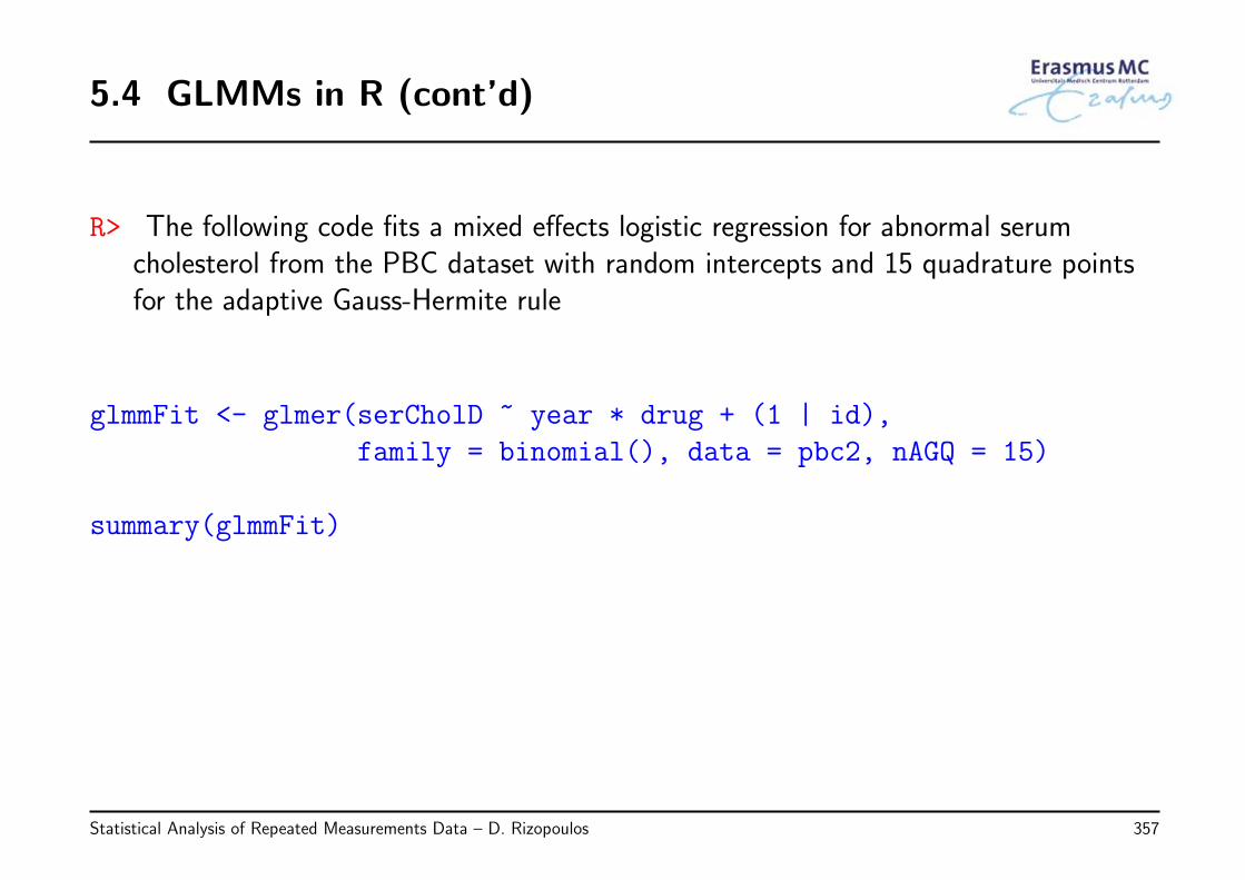
5.4 GLMMs in R (cont’d)
R> The following code fits a mixed effects logistic regression for abnormal serumcholesterol from the PBC dataset with random intercepts and 15 quadrature pointsfor the adaptive Gauss-Hermite rule
glmmFit <- glmer(serCholD ~ year * drug + (1 | id),
family = binomial(), data = pbc2, nAGQ = 15)
summary(glmmFit)
Statistical Analysis of Repeated Measurements Data – D. Rizopoulos 357
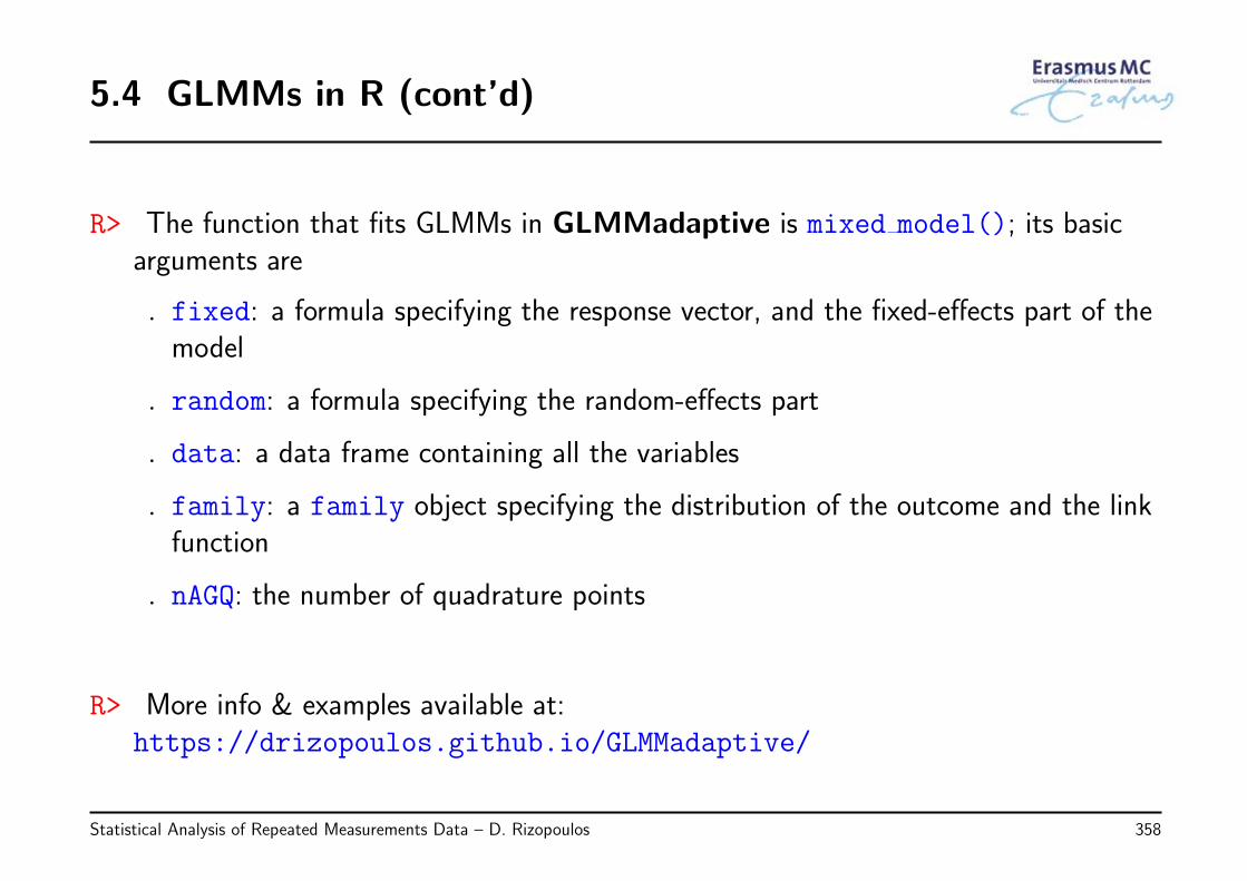
5.4 GLMMs in R (cont’d)
R> The function that fits GLMMs in GLMMadaptive is mixed model(); its basicarguments are
◃ fixed: a formula specifying the response vector, and the fixed-effects part of themodel
◃ random: a formula specifying the random-effects part
◃ data: a data frame containing all the variables
◃ family: a family object specifying the distribution of the outcome and the linkfunction
◃ nAGQ: the number of quadrature points
R> More info & examples available at:https://drizopoulos.github.io/GLMMadaptive/
Statistical Analysis of Repeated Measurements Data – D. Rizopoulos 358
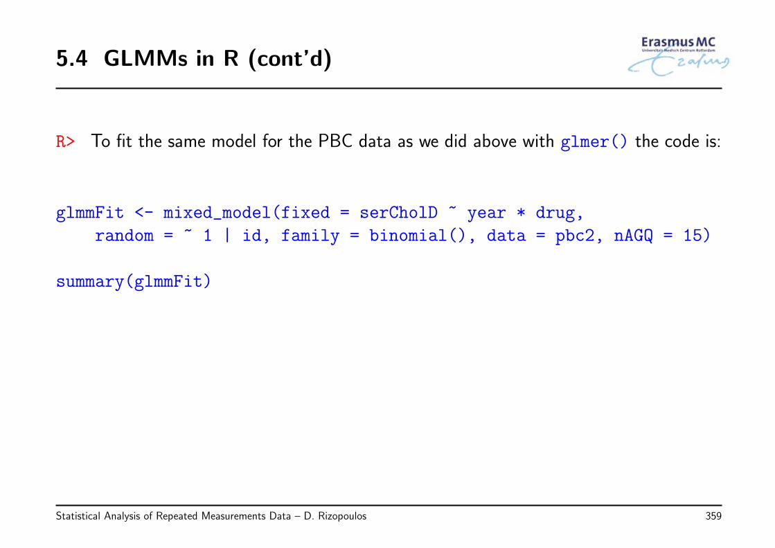
5.4 GLMMs in R (cont’d)
R> To fit the same model for the PBC data as we did above with glmer() the code is:
glmmFit <- mixed_model(fixed = serCholD ~ year * drug,
random = ~ 1 | id, family = binomial(), data = pbc2, nAGQ = 15)
summary(glmmFit)
Statistical Analysis of Repeated Measurements Data – D. Rizopoulos 359
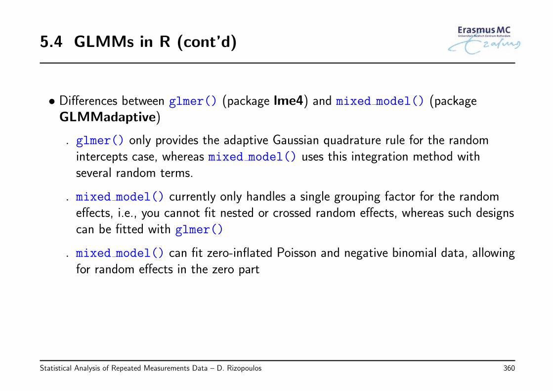
5.4 GLMMs in R (cont’d)
• Differences between glmer() (package lme4) and mixed model() (packageGLMMadaptive)
◃ glmer() only provides the adaptive Gaussian quadrature rule for the randomintercepts case, whereas mixed model() uses this integration method withseveral random terms.
◃ mixed model() currently only handles a single grouping factor for the randomeffects, i.e., you cannot fit nested or crossed random effects, whereas such designscan be fitted with glmer()
◃ mixed model() can fit zero-inflated Poisson and negative binomial data, allowingfor random effects in the zero part
Statistical Analysis of Repeated Measurements Data – D. Rizopoulos 360
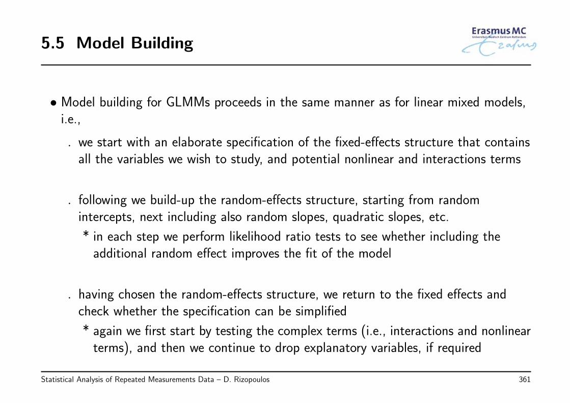
5.5 Model Building
• Model building for GLMMs proceeds in the same manner as for linear mixed models,i.e.,
◃ we start with an elaborate specification of the fixed-effects structure that containsall the variables we wish to study, and potential nonlinear and interactions terms
◃ following we build-up the random-effects structure, starting from randomintercepts, next including also random slopes, quadratic slopes, etc.
* in each step we perform likelihood ratio tests to see whether including theadditional random effect improves the fit of the model
◃ having chosen the random-effects structure, we return to the fixed effects andcheck whether the specification can be simplified
* again we first start by testing the complex terms (i.e., interactions and nonlinearterms), and then we continue to drop explanatory variables, if required
Statistical Analysis of Repeated Measurements Data – D. Rizopoulos 361
5.5 Model Building (cont’d)
• Nevertheless, quite often, and especially for dichotomous data, extending therandom-effects structure may lead to numerical/computational problems
◃ this is because dichotomous data contain the least amount of information
• Hence, for dichotomous data and when we have few to moderate number of repeatedmeasurements per subject, we often can only fit random intercepts models
Statistical Analysis of Repeated Measurements Data – D. Rizopoulos 362
5.6 Hypothesis Testing
• Having fitted a GLMM with maximum likelihood, testing of either the fixed- orrandom-effects structure proceeds in a similar manner as in linear mixed models
• Important difference: in GLMMs we do not have REML we always work with fullmaximum likelihood
◃ when we want to test the random-effects, the fixed-effects structure is alsoallowed to be different (though comparing nested models is a requirement forusing the standard tests)
Statistical Analysis of Repeated Measurements Data – D. Rizopoulos 363
5.6 Hypothesis Testing (cont’d)
• Example: In the PBC dataset and for the dichotomous longitudinal outcome highserum cholesterol levels (defined as before as above the threshold of 210 mg/dL), wefit a model that postulates
◃ fixed effects:
* main effects of time, treatment, and sex
* interaction effects between time and treatment, and between drug and sex
◃ random effects: random intercepts
We are interested in testing whether the model can be simplified by dropping theinteraction terms
Statistical Analysis of Repeated Measurements Data – D. Rizopoulos 364
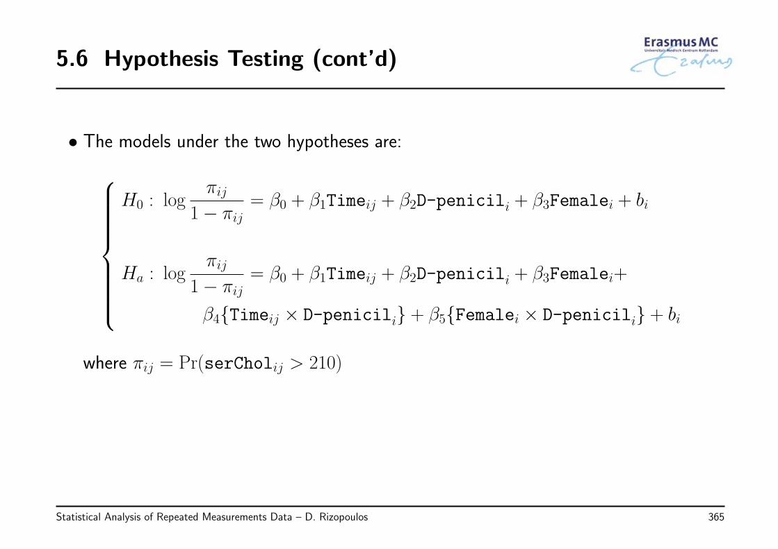
5.6 Hypothesis Testing (cont’d)
• The models under the two hypotheses are:
H0 : logπij
1− πij= β0 + β1Timeij + β2D-penicili + β3Femalei + bi
Ha : logπij
1− πij= β0 + β1Timeij + β2D-penicili + β3Femalei+
β4{Timeij × D-penicili} + β5{Femalei × D-penicili} + bi
where πij = Pr(serCholij > 210)
Statistical Analysis of Repeated Measurements Data – D. Rizopoulos 365
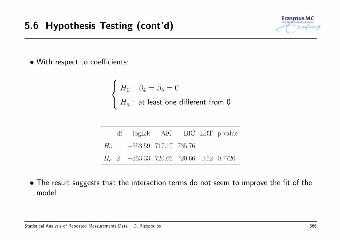
5.6 Hypothesis Testing (cont’d)
• With respect to coefficients:H0 : β4 = β5 = 0
Ha : at least one different from 0
df logLik AIC BIC LRT p-value
H0 −353.59 717.17 735.76
Ha 2 −353.33 720.66 720.66 0.52 0.7726
• The result suggests that the interaction terms do not seem to improve the fit of themodel
Statistical Analysis of Repeated Measurements Data – D. Rizopoulos 366
5.6 Hypothesis Testing (cont’d)
• Similarly to previous chapters, when we want to test non-nested models we can useinformation criteria, i.e., the AIC or the BIC
Statistical Analysis of Repeated Measurements Data – D. Rizopoulos 367
5.7 Review of Key Points
• GLMMs are the analogue of linear mixed models for categorical data
◃ we include random effects in the linear predictor to account for the correlations inthe outcomes belonging to the same group/cluster
• Features of GLMMs
◃ these models provide a complete specification of the distribution of thegrouped/longitudinal outcome – contrary to GEE, which is a semi-parametricmethod
◃ interpretation of parameters is conditional on the random effects – contrary toGEE, which provide coefficients with a marginal interpretation
Statistical Analysis of Repeated Measurements Data – D. Rizopoulos 368
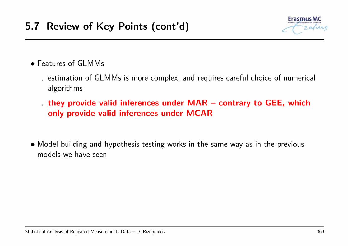
5.7 Review of Key Points (cont’d)
• Features of GLMMs
◃ estimation of GLMMs is more complex, and requires careful choice of numericalalgorithms
◃ they provide valid inferences under MAR – contrary to GEE, whichonly provide valid inferences under MCAR
• Model building and hypothesis testing works in the same way as in the previousmodels we have seen
Statistical Analysis of Repeated Measurements Data – D. Rizopoulos 369
Chapter 6
Statistical Analysis with Incomplete Grouped Data
Statistical Analysis of Repeated Measurements Data – D. Rizopoulos 370
6.1 Missing Data in Longitudinal Studies
A major challenge for the analysis of grouped/longitudinaldata is missing data
◃ Even though studies are designed to collect data on every subject at a set ofprespecified follow-up times
◃ Subjects often miss some of their planned measurements for a variety of reasons
Statistical Analysis of Repeated Measurements Data – D. Rizopoulos 371
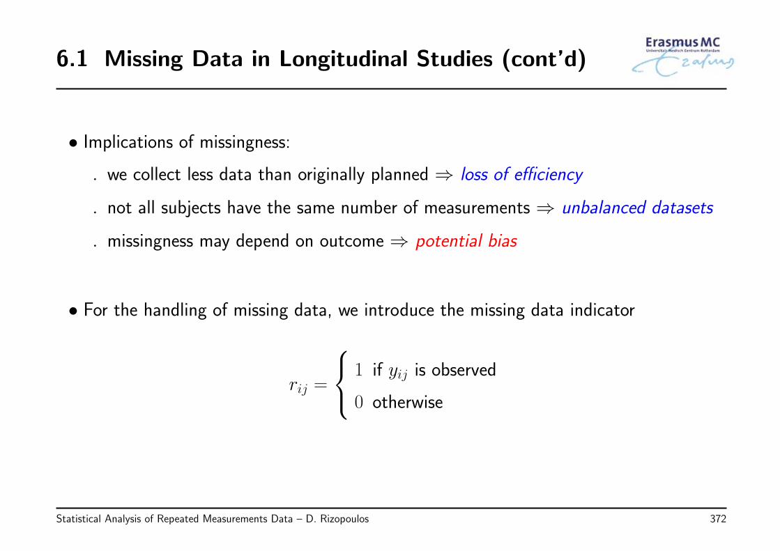
6.1 Missing Data in Longitudinal Studies (cont’d)
• Implications of missingness:
◃ we collect less data than originally planned ⇒ loss of efficiency
◃ not all subjects have the same number of measurements ⇒ unbalanced datasets
◃ missingness may depend on outcome ⇒ potential bias
• For the handling of missing data, we introduce the missing data indicator
rij =
1 if yij is observed
0 otherwise
Statistical Analysis of Repeated Measurements Data – D. Rizopoulos 372
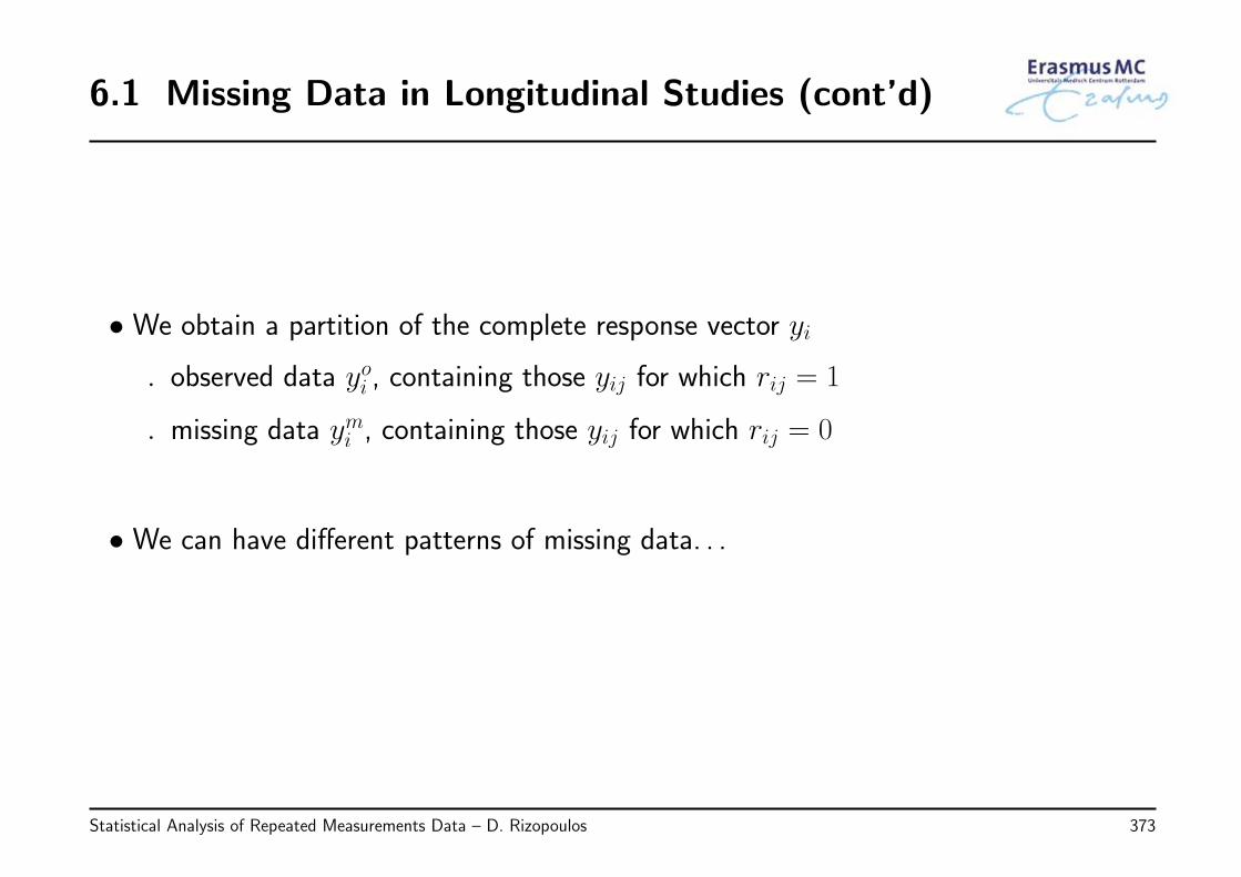
6.1 Missing Data in Longitudinal Studies (cont’d)
• We obtain a partition of the complete response vector yi
◃ observed data yoi , containing those yij for which rij = 1
◃ missing data ymi , containing those yij for which rij = 0
• We can have different patterns of missing data. . .
Statistical Analysis of Repeated Measurements Data – D. Rizopoulos 373
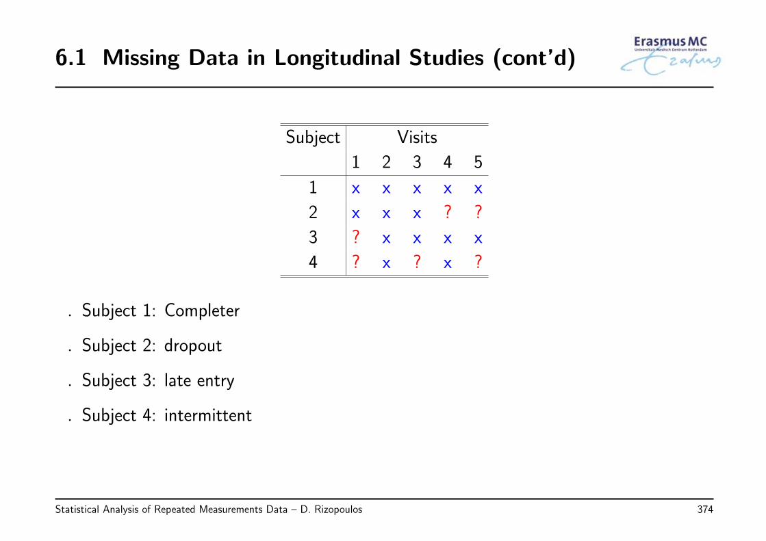
6.1 Missing Data in Longitudinal Studies (cont’d)
Subject Visits
1 2 3 4 5
1 x x x x x
2 x x x ? ?
3 ? x x x x
4 ? x ? x ?
◃ Subject 1: Completer
◃ Subject 2: dropout
◃ Subject 3: late entry
◃ Subject 4: intermittent
Statistical Analysis of Repeated Measurements Data – D. Rizopoulos 374
6.1 Missing Data in Longitudinal Studies (cont’d)
• When the focus is only on dropout the notation can be simplified
◃ Discrete dropout time: rdi = 1 +ni∑j=1
rij (ordinal variable)
◃ Continuous dropout time: T ∗i denotes the time to dropout
• Focusing on dropout only is justifiable because often intermittent missing data can beconsidered MAR (definition of MAR follows. . . )
Statistical Analysis of Repeated Measurements Data – D. Rizopoulos 375
6.2 Missing Data Mechanisms
• To describe the probabilistic relation between the measurement and missingnessprocesses Rubin (1976, Biometrika) has introduced three mechanisms
• Missing Completely At Random (MCAR): The probability that responses are missingis unrelated to both yoi and ymi
p(ri | yoi , ymi ) = p(ri)
• Examples
◃ subjects go out of the study after providing a pre-determined number ofmeasurements
◃ laboratory measurements are lost due to equipment malfunction
Statistical Analysis of Repeated Measurements Data – D. Rizopoulos 376
6.2 Missing Data Mechanisms (cont’d)
• Features of MCAR:
◃ The observed data yoi can be considered a random sample of the complete data yi
◃ We can use any statistical procedure that is valid for complete data
* sample averages per time point
* linear regression, ignoring the correlation (consistent, but not efficient)
* t-test at the last time point
* . . .
Statistical Analysis of Repeated Measurements Data – D. Rizopoulos 377

6.2 Missing Data Mechanisms (cont’d)
• Missing At Random (MAR): The probability that responses are missing is related toyoi , but is unrelated to ymi
p(ri | yoi , ymi ) = p(ri | yoi )
• Examples
◃ study protocol requires patients whose response value exceeds a threshold to beremoved from the study
◃ physicians give rescue medication to patients who do not respond to treatment
Statistical Analysis of Repeated Measurements Data – D. Rizopoulos 378
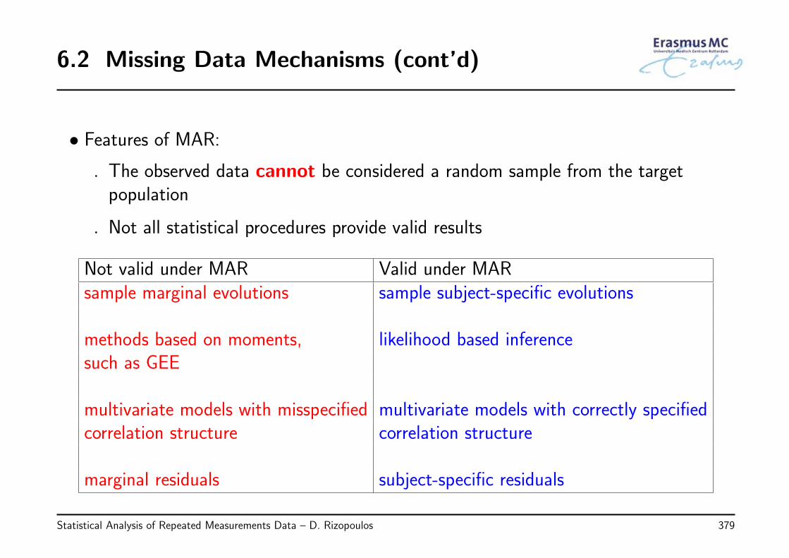
6.2 Missing Data Mechanisms (cont’d)
• Features of MAR:
◃ The observed data cannot be considered a random sample from the targetpopulation
◃ Not all statistical procedures provide valid results
Not valid under MAR Valid under MARsample marginal evolutions sample subject-specific evolutions
methods based on moments, likelihood based inferencesuch as GEE
multivariate models with misspecified multivariate models with correctly specifiedcorrelation structure correlation structure
marginal residuals subject-specific residuals
Statistical Analysis of Repeated Measurements Data – D. Rizopoulos 379
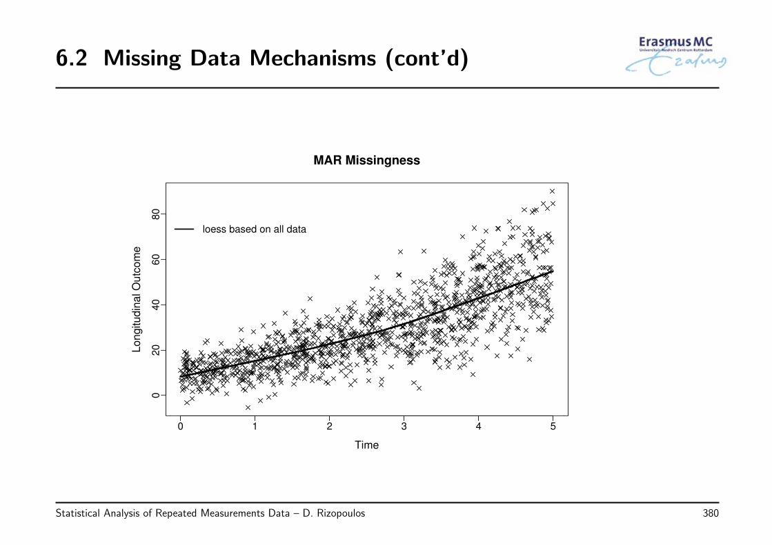
6.2 Missing Data Mechanisms (cont’d)
0 1 2 3 4 5
020
40
60
80
MAR Missingness
Time
Lo
ng
itu
din
al O
utc
om
e
loess based on all data
Statistical Analysis of Repeated Measurements Data – D. Rizopoulos 380
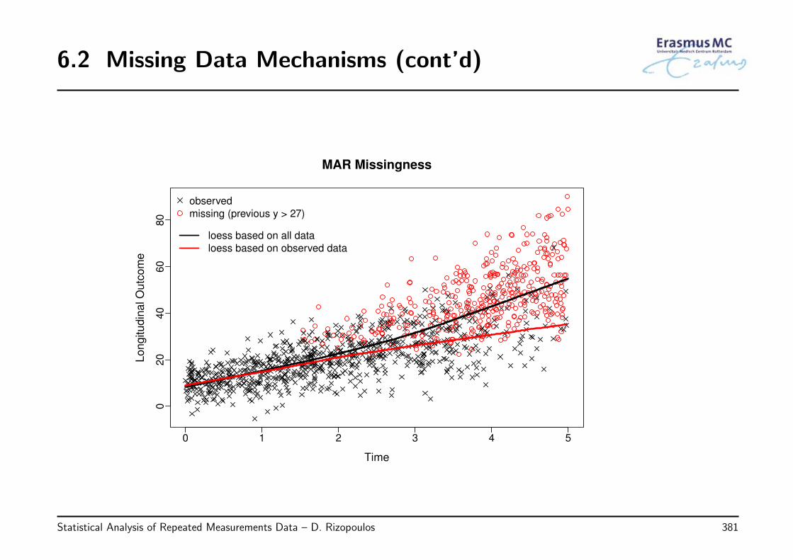
6.2 Missing Data Mechanisms (cont’d)
0 1 2 3 4 5
020
40
60
80
MAR Missingness
Time
Lo
ng
itu
din
al O
utc
om
e
observed
missing (previous y > 27)
loess based on all data
loess based on observed data
Statistical Analysis of Repeated Measurements Data – D. Rizopoulos 381
6.2 Missing Data Mechanisms (cont’d)
• To illustrate the important implications of incomplete data, let’s return to theresiduals plots we have seen in Chapter 2 (pp.138–142)
• We had fitted the following model to the PBC datasetlog(serBilirij) = β0 + β1Timeij + β2Femalei + β3Agei+
β4{D-penicili × Timeij} + β5{Femalei × Timeij} + εij
εi ∼ N (0, Vi) Vi has a continuous AR1 structure
and the scatterplot of the standardized residuals versus fitted values was
Statistical Analysis of Repeated Measurements Data – D. Rizopoulos 382
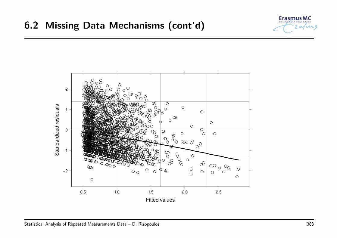
6.2 Missing Data Mechanisms (cont’d)
Fitted values
Sta
nd
ard
ized
resid
ua
ls
−2
−1
0
1
2
0.5 1.0 1.5 2.0 2.5
Statistical Analysis of Repeated Measurements Data – D. Rizopoulos 383
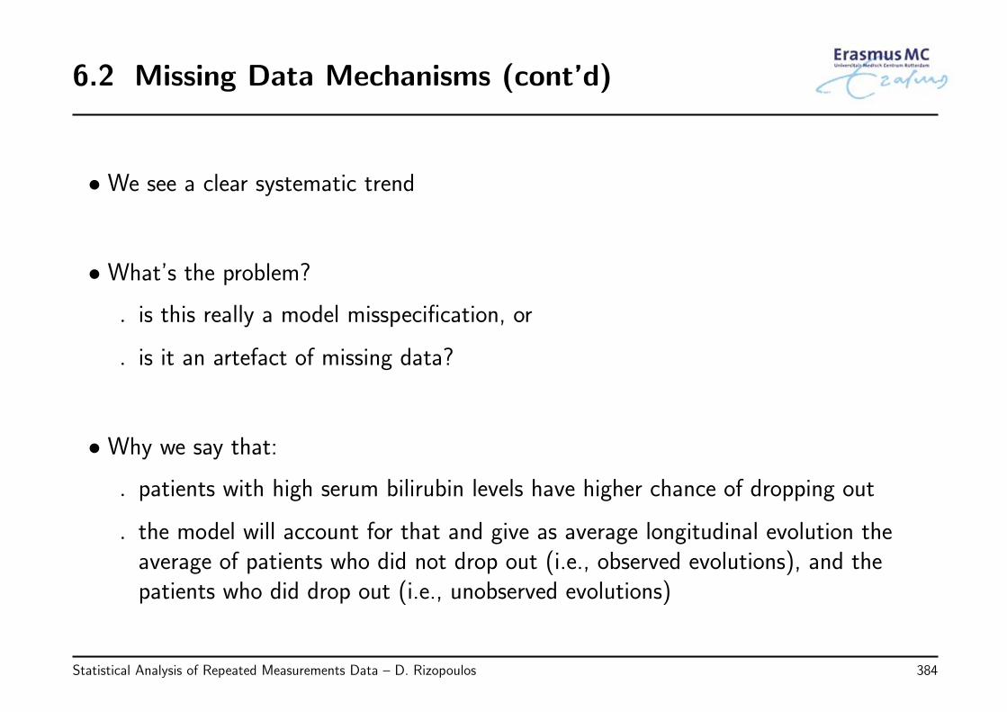
6.2 Missing Data Mechanisms (cont’d)
• We see a clear systematic trend
• What’s the problem?
◃ is this really a model misspecification, or
◃ is it an artefact of missing data?
• Why we say that:
◃ patients with high serum bilirubin levels have higher chance of dropping out
◃ the model will account for that and give as average longitudinal evolution theaverage of patients who did not drop out (i.e., observed evolutions), and thepatients who did drop out (i.e., unobserved evolutions)
Statistical Analysis of Repeated Measurements Data – D. Rizopoulos 384
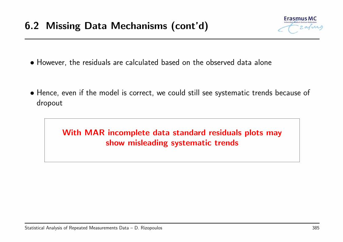
6.2 Missing Data Mechanisms (cont’d)
• However, the residuals are calculated based on the observed data alone
• Hence, even if the model is correct, we could still see systematic trends because ofdropout
With MAR incomplete data standard residuals plots mayshow misleading systematic trends
Statistical Analysis of Repeated Measurements Data – D. Rizopoulos 385
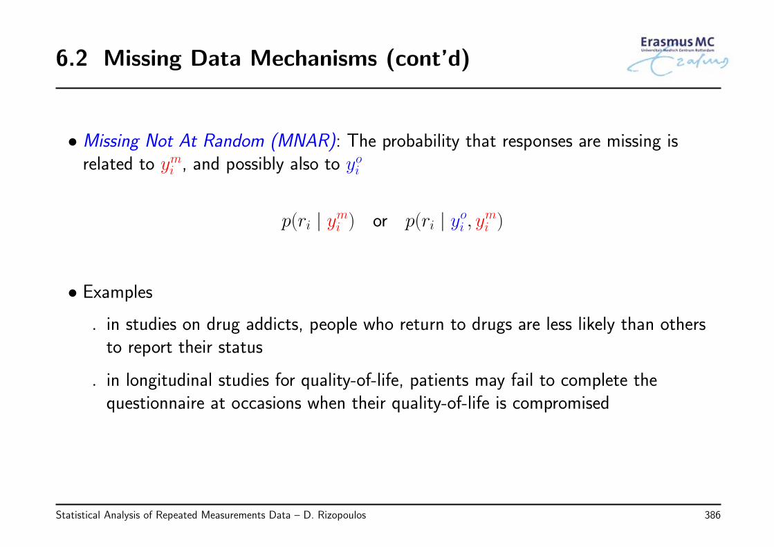
6.2 Missing Data Mechanisms (cont’d)
• Missing Not At Random (MNAR): The probability that responses are missing isrelated to ymi , and possibly also to yoi
p(ri | ymi ) or p(ri | yoi , ymi )
• Examples
◃ in studies on drug addicts, people who return to drugs are less likely than othersto report their status
◃ in longitudinal studies for quality-of-life, patients may fail to complete thequestionnaire at occasions when their quality-of-life is compromised
Statistical Analysis of Repeated Measurements Data – D. Rizopoulos 386
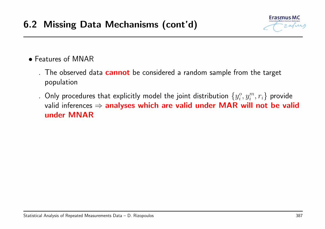
6.2 Missing Data Mechanisms (cont’d)
• Features of MNAR
◃ The observed data cannot be considered a random sample from the targetpopulation
◃ Only procedures that explicitly model the joint distribution {yoi , ymi , ri} providevalid inferences ⇒ analyses which are valid under MAR will not be validunder MNAR
Statistical Analysis of Repeated Measurements Data – D. Rizopoulos 387
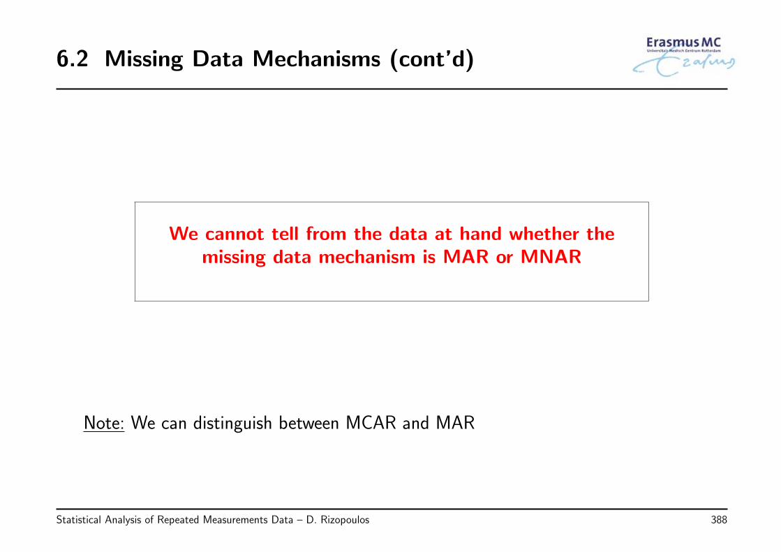
6.2 Missing Data Mechanisms (cont’d)
We cannot tell from the data at hand whether themissing data mechanism is MAR or MNAR
Note: We can distinguish between MCAR and MAR
Statistical Analysis of Repeated Measurements Data – D. Rizopoulos 388
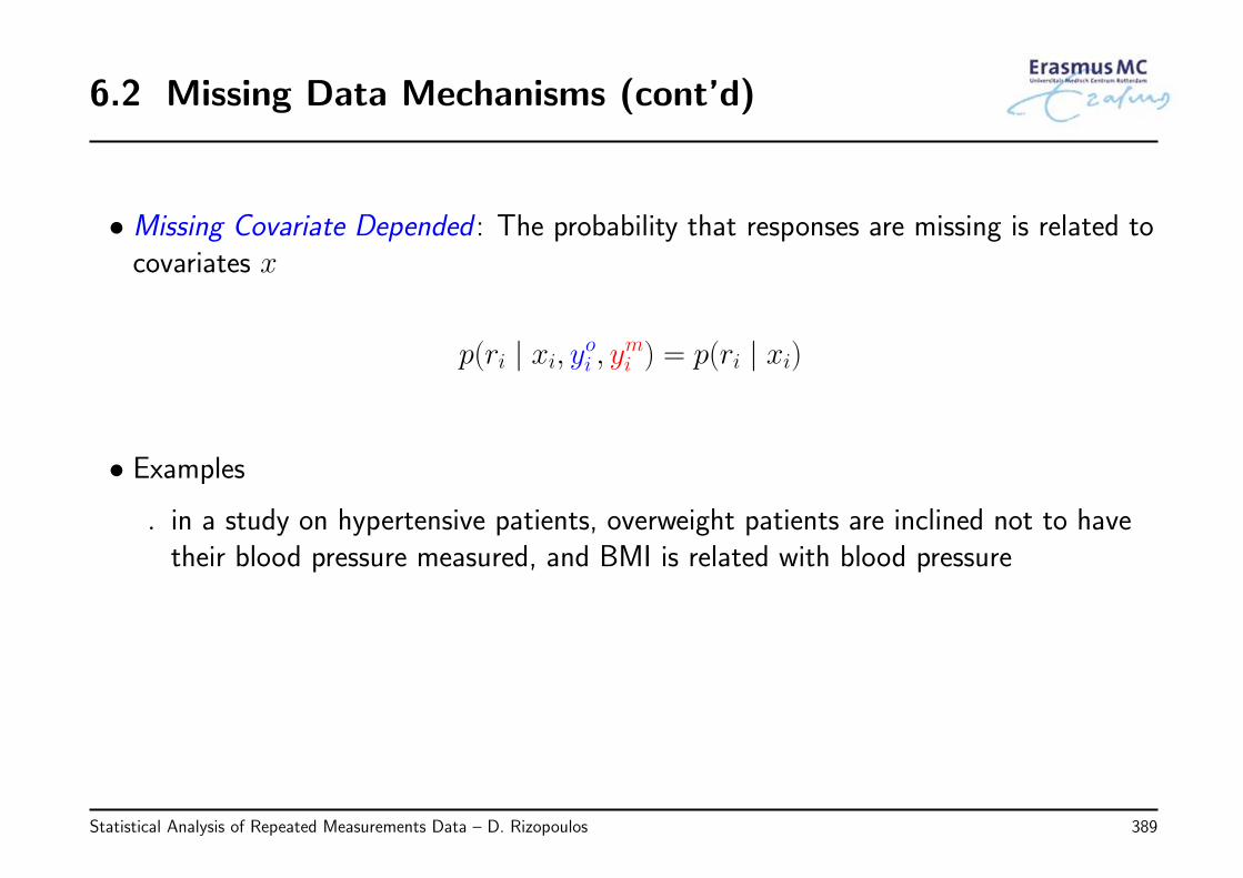
6.2 Missing Data Mechanisms (cont’d)
• Missing Covariate Depended : The probability that responses are missing is related tocovariates x
p(ri | xi, yoi , ymi ) = p(ri | xi)
• Examples
◃ in a study on hypertensive patients, overweight patients are inclined not to havetheir blood pressure measured, and BMI is related with blood pressure
Statistical Analysis of Repeated Measurements Data – D. Rizopoulos 389
6.2 Missing Data Mechanisms (cont’d)
• Features of Missing Covariate Depended
◃ If we do not include the covariates that drive the missingness process in theregression model for the longitudinal outcome Y , and these covariates areassociated with Y , then we obtain an MNAR mechanism
Statistical Analysis of Repeated Measurements Data – D. Rizopoulos 390
6.3 Analysis with Incomplete Data
• We have seen what the implications of missingness are and how they complicatematters
• To this end, several approaches have been proposed to account for missing data
◃ depending on the missing data mechanism, not all of them providevalid results!
Statistical Analysis of Repeated Measurements Data – D. Rizopoulos 391
6.3 Analysis with Incomplete Data (cont’d)
• Complete Cases Analysis
◃ General idea: Restrict analyses to only those subjects for which allmeasurements are observed
◃ Advantages:
* very simple to implement
* standard software can be used
Disadvantages:
* substantial loss of information
* valid inferences only when missingness is completely unrelated to the outcome(i.e., MCAR)
Statistical Analysis of Repeated Measurements Data – D. Rizopoulos 392
6.3 Analysis with Incomplete Data (cont’d)
• Last Observation Carried Forward (LOCF)
◃ General idea: Any missing value is replaced by the last observed value
◃ Advantages:
* very simple to implement
* standard software can be used
Disadvantages:
* extremely strong assumption that a subject’s measurement stays at the samelevel as soon as he/she is not observed
* even if the mechanism is MCAR, LOCF may not provide valid results
* overestimates precision
Statistical Analysis of Repeated Measurements Data – D. Rizopoulos 393
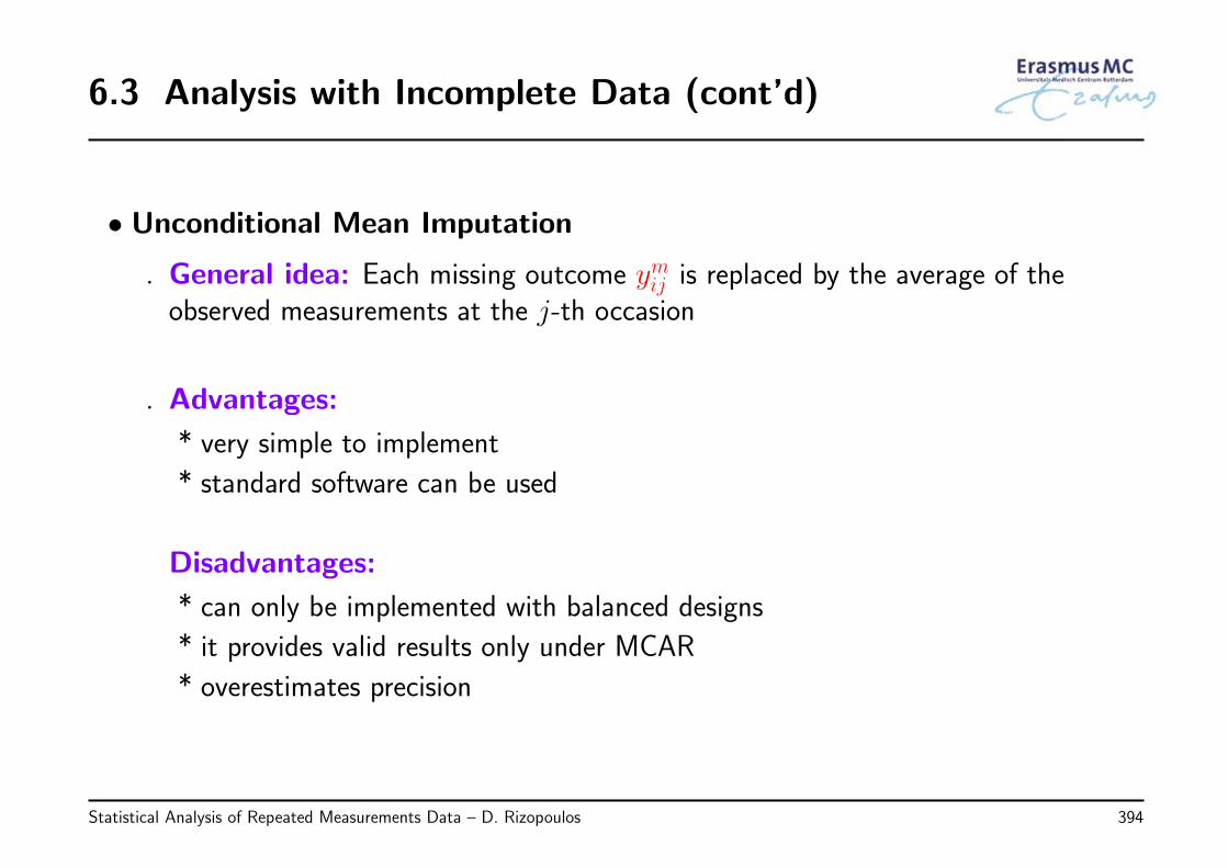
6.3 Analysis with Incomplete Data (cont’d)
• Unconditional Mean Imputation
◃ General idea: Each missing outcome ymij is replaced by the average of theobserved measurements at the j-th occasion
◃ Advantages:
* very simple to implement
* standard software can be used
Disadvantages:
* can only be implemented with balanced designs
* it provides valid results only under MCAR
* overestimates precision
Statistical Analysis of Repeated Measurements Data – D. Rizopoulos 394
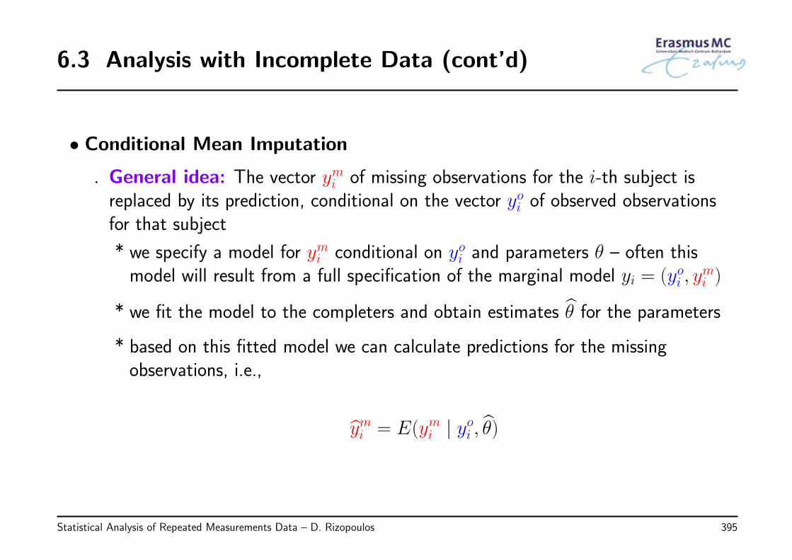
6.3 Analysis with Incomplete Data (cont’d)
• Conditional Mean Imputation
◃ General idea: The vector ymi of missing observations for the i-th subject isreplaced by its prediction, conditional on the vector yoi of observed observationsfor that subject
* we specify a model for ymi conditional on yoi and parameters θ – often thismodel will result from a full specification of the marginal model yi = (yoi , y
mi )
* we fit the model to the completers and obtain estimates θ for the parameters
* based on this fitted model we can calculate predictions for the missingobservations, i.e.,
ymi = E(ymi | yoi , θ)
Statistical Analysis of Repeated Measurements Data – D. Rizopoulos 395
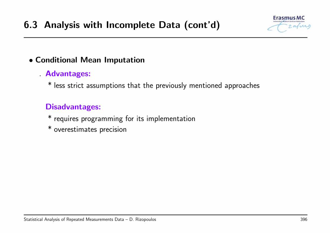
6.3 Analysis with Incomplete Data (cont’d)
• Conditional Mean Imputation
◃ Advantages:
* less strict assumptions that the previously mentioned approaches
Disadvantages:
* requires programming for its implementation
* overestimates precision
Statistical Analysis of Repeated Measurements Data – D. Rizopoulos 396
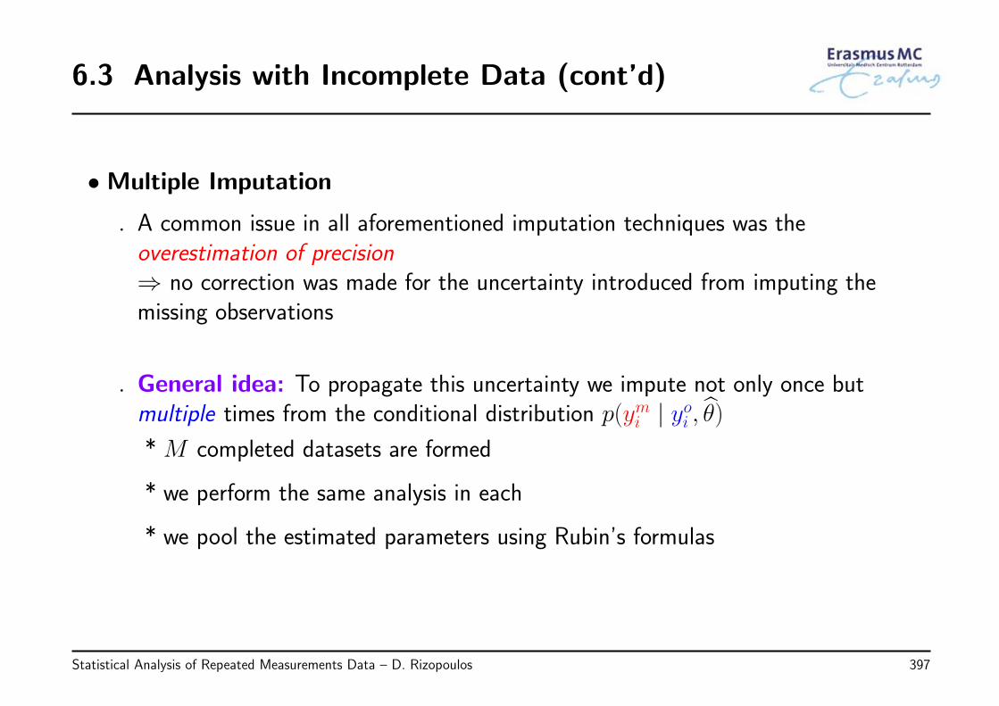
6.3 Analysis with Incomplete Data (cont’d)
• Multiple Imputation
◃ A common issue in all aforementioned imputation techniques was theoverestimation of precision⇒ no correction was made for the uncertainty introduced from imputing themissing observations
◃ General idea: To propagate this uncertainty we impute not only once butmultiple times from the conditional distribution p(ymi | yoi , θ)* M completed datasets are formed
* we perform the same analysis in each
* we pool the estimated parameters using Rubin’s formulas
Statistical Analysis of Repeated Measurements Data – D. Rizopoulos 397
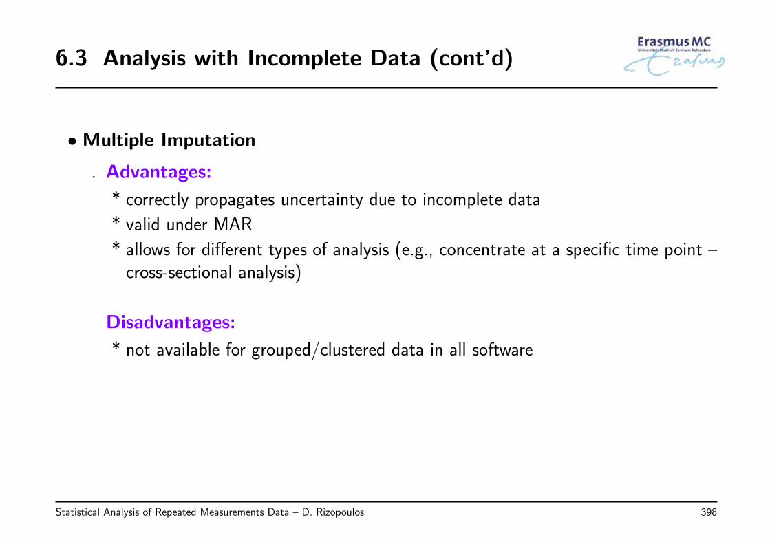
6.3 Analysis with Incomplete Data (cont’d)
• Multiple Imputation
◃ Advantages:
* correctly propagates uncertainty due to incomplete data
* valid under MAR
* allows for different types of analysis (e.g., concentrate at a specific time point –cross-sectional analysis)
Disadvantages:
* not available for grouped/clustered data in all software
Statistical Analysis of Repeated Measurements Data – D. Rizopoulos 398
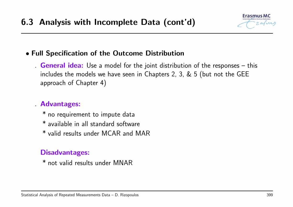
6.3 Analysis with Incomplete Data (cont’d)
• Full Specification of the Outcome Distribution
◃ General idea: Use a model for the joint distribution of the responses – thisincludes the models we have seen in Chapters 2, 3, & 5 (but not the GEEapproach of Chapter 4)
◃ Advantages:
* no requirement to impute data
* available in all standard software
* valid results under MCAR and MAR
Disadvantages:
* not valid results under MNAR
Statistical Analysis of Repeated Measurements Data – D. Rizopoulos 399
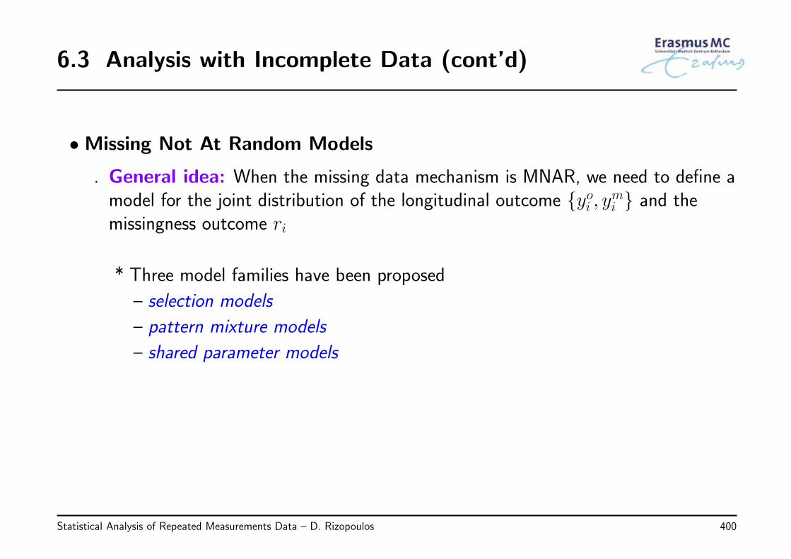
6.3 Analysis with Incomplete Data (cont’d)
• Missing Not At Random Models
◃ General idea: When the missing data mechanism is MNAR, we need to define amodel for the joint distribution of the longitudinal outcome {yoi , ymi } and themissingness outcome ri
* Three model families have been proposed
– selection models
– pattern mixture models
– shared parameter models
Statistical Analysis of Repeated Measurements Data – D. Rizopoulos 400
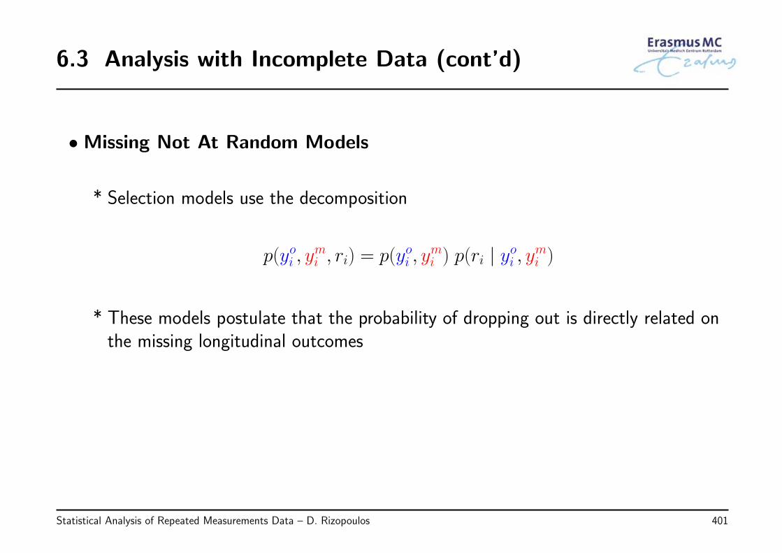
6.3 Analysis with Incomplete Data (cont’d)
• Missing Not At Random Models
* Selection models use the decomposition
p(yoi , ymi , ri) = p(yoi , y
mi ) p(ri | yoi , ymi )
* These models postulate that the probability of dropping out is directly related onthe missing longitudinal outcomes
Statistical Analysis of Repeated Measurements Data – D. Rizopoulos 401
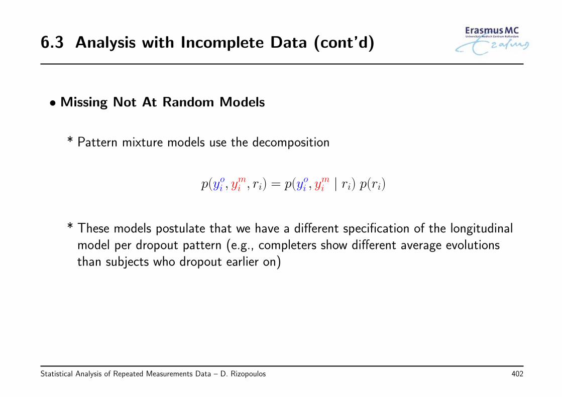
6.3 Analysis with Incomplete Data (cont’d)
• Missing Not At Random Models
* Pattern mixture models use the decomposition
p(yoi , ymi , ri) = p(yoi , y
mi | ri) p(ri)
* These models postulate that we have a different specification of the longitudinalmodel per dropout pattern (e.g., completers show different average evolutionsthan subjects who dropout earlier on)
Statistical Analysis of Repeated Measurements Data – D. Rizopoulos 402
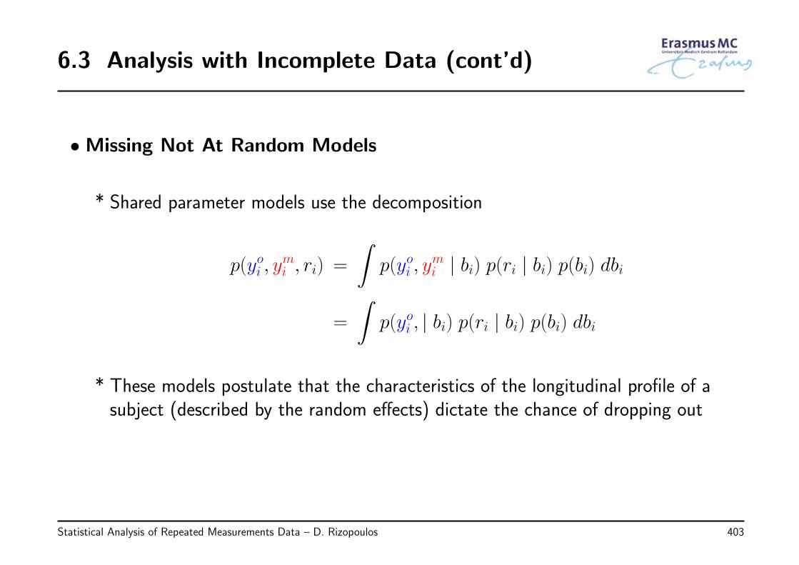
6.3 Analysis with Incomplete Data (cont’d)
• Missing Not At Random Models
* Shared parameter models use the decomposition
p(yoi , ymi , ri) =
∫p(yoi , y
mi | bi) p(ri | bi) p(bi) dbi
=
∫p(yoi , | bi) p(ri | bi) p(bi) dbi
* These models postulate that the characteristics of the longitudinal profile of asubject (described by the random effects) dictate the chance of dropping out
Statistical Analysis of Repeated Measurements Data – D. Rizopoulos 403
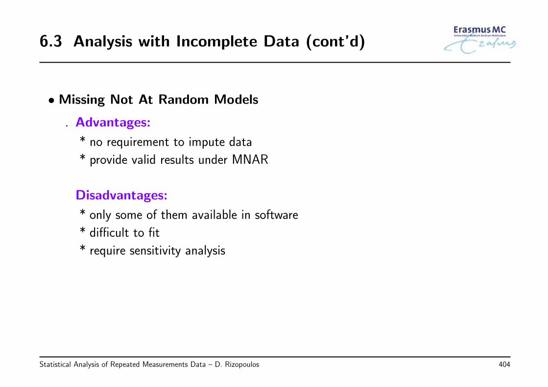
6.3 Analysis with Incomplete Data (cont’d)
• Missing Not At Random Models
◃ Advantages:
* no requirement to impute data
* provide valid results under MNAR
Disadvantages:
* only some of them available in software
* difficult to fit
* require sensitivity analysis
Statistical Analysis of Repeated Measurements Data – D. Rizopoulos 404
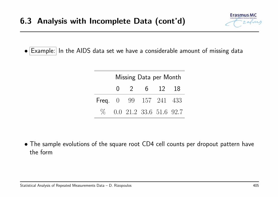
6.3 Analysis with Incomplete Data (cont’d)
• Example: In the AIDS data set we have a considerable amount of missing data
Missing Data per Month
0 2 6 12 18
Freq. 0 99 157 241 433
% 0.0 21.2 33.6 51.6 92.7
• The sample evolutions of the square root CD4 cell counts per dropout pattern havethe form
Statistical Analysis of Repeated Measurements Data – D. Rizopoulos 405
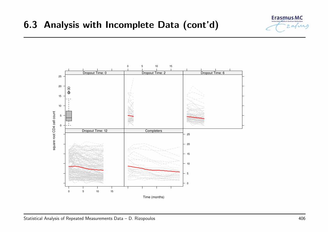
6.3 Analysis with Incomplete Data (cont’d)
Time (months)
sq
ua
re r
oot
CD
4 c
ell
co
un
t
0
5
10
15
20
25
Dropout Time: 0
0 5 10 15
Dropout Time: 2 Dropout Time: 6
0 5 10 15
Dropout Time: 12
0
5
10
15
20
25
Completers
Statistical Analysis of Repeated Measurements Data – D. Rizopoulos 406
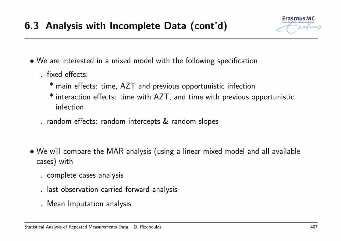
6.3 Analysis with Incomplete Data (cont’d)
• We are interested in a mixed model with the following specification
◃ fixed effects:
* main effects: time, AZT and previous opportunistic infection
* interaction effects: time with AZT, and time with previous opportunisticinfection
◃ random effects: random intercepts & random slopes
• We will compare the MAR analysis (using a linear mixed model and all availablecases) with
◃ complete cases analysis
◃ last observation carried forward analysis
◃ Mean Imputation analysis
Statistical Analysis of Repeated Measurements Data – D. Rizopoulos 407
6.3 Analysis with Incomplete Data (cont’d)
• The following boxplots illustrate the distribution of square root CD4 cell counts underthe different strategies
Statistical Analysis of Repeated Measurements Data – D. Rizopoulos 408
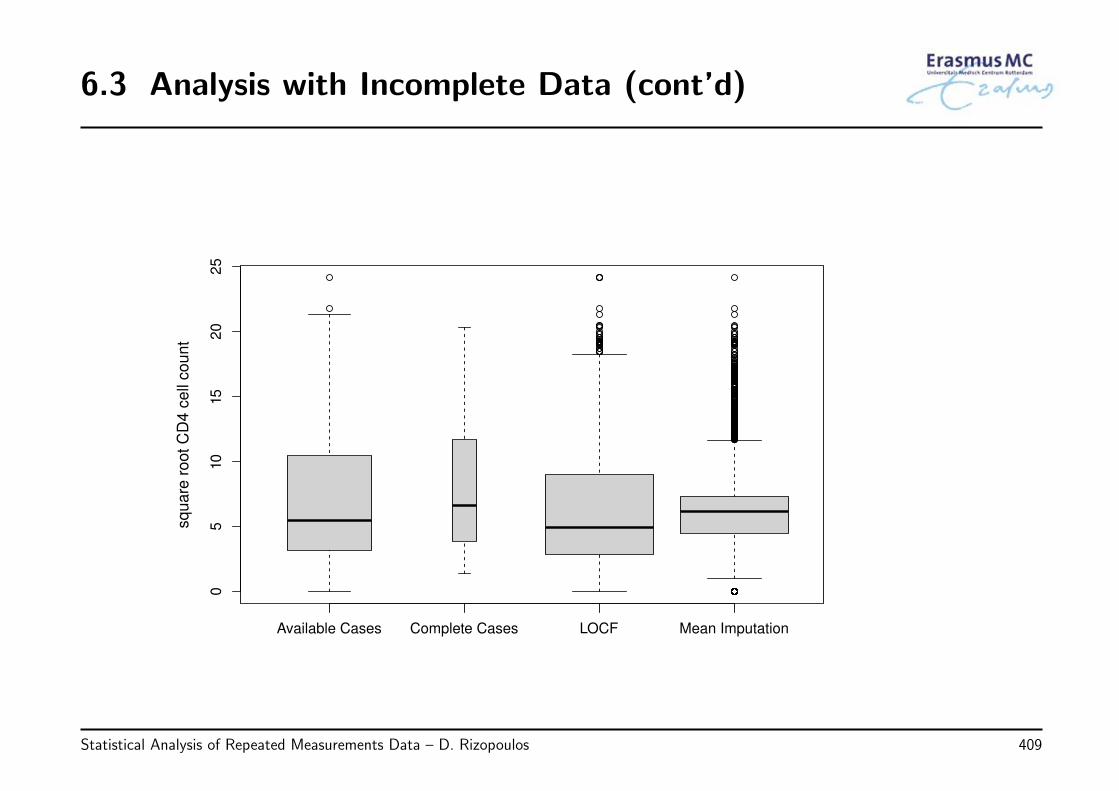
6.3 Analysis with Incomplete Data (cont’d)
Available Cases Complete Cases LOCF Mean Imputation
05
10
15
20
25
sq
ua
re r
oot
CD
4 c
ell
co
un
t
Statistical Analysis of Repeated Measurements Data – D. Rizopoulos 409
6.3 Analysis with Incomplete Data (cont’d)
• The following figure illustrates the estimated coefficients and the corresponding 95%confidence intervals from the four mixed models fitted to the different versions of thesquare root CD4 cell counts variable
Statistical Analysis of Repeated Measurements Data – D. Rizopoulos 410
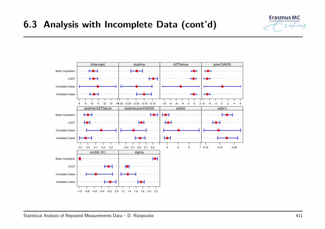
6.3 Analysis with Incomplete Data (cont’d)
Available Cases
Complete Cases
LOCF
Mean Imputation
8 9 10 11 12 13 14
(Intercept)
−0.30 −0.25 −0.20 −0.15 −0.10
obstime
−10 −8 −6 −4 −2 0 2
AZTfailure
−6 −4 −2 0 2 4 6
prevOIAIDS
Available Cases
Complete Cases
LOCF
Mean Imputation
−0.1 0.0 0.1 0.2 0.3
obstime:AZTfailure
−0.2 −0.1 0.0 0.1 0.2
obstime:prevOIAIDS
4 5 6 7
sd(b0)
0.10 0.15 0.20
sd(b1)
Available Cases
Complete Cases
LOCF
Mean Imputation
−1.0 −0.8 −0.6 −0.4 −0.2 0.0
cor(b0, b1)
1.2 1.4 1.6 1.8 2.0 2.2
sigma
Statistical Analysis of Repeated Measurements Data – D. Rizopoulos 411
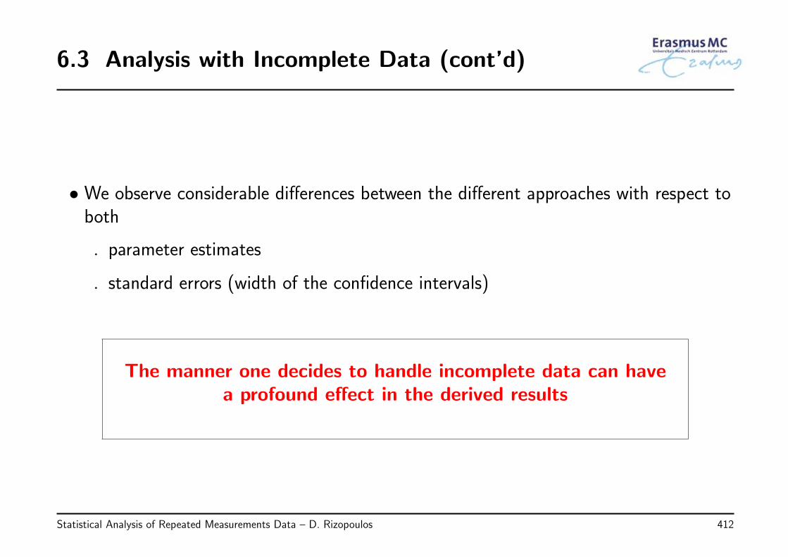
6.3 Analysis with Incomplete Data (cont’d)
• We observe considerable differences between the different approaches with respect toboth
◃ parameter estimates
◃ standard errors (width of the confidence intervals)
The manner one decides to handle incomplete data can havea profound effect in the derived results
Statistical Analysis of Repeated Measurements Data – D. Rizopoulos 412
6.4 Summary
• It is now universally recognized that the default type of statistical analysis shouldprovide valid results under MAR
• Hence, whenever we have missing data in the outcome, it is advisable to employ afull-likelihood approach based on the models we have seen for continuous andcategorical responses⇒ No need for (multiple) imputation
• However, to be protected we need an appropriate specification of the jointdistribution of the data
Statistical Analysis of Repeated Measurements Data – D. Rizopoulos 413
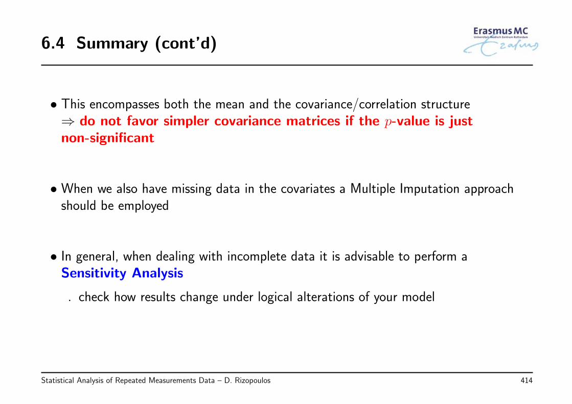
6.4 Summary (cont’d)
• This encompasses both the mean and the covariance/correlation structure⇒ do not favor simpler covariance matrices if the p-value is justnon-significant
• When we also have missing data in the covariates a Multiple Imputation approachshould be employed
• In general, when dealing with incomplete data it is advisable to perform aSensitivity Analysis
◃ check how results change under logical alterations of your model
Statistical Analysis of Repeated Measurements Data – D. Rizopoulos 414
6.5 Review of Key Points
• Missing data pose an important complication in the analysis of clustered/groupeddata
◃ loss of efficiency
◃ potential bias
• Need to carefully consider the reasons why data are missing
◃ MCAR ⇒ missingness not related to the outcome
◃ MAR ⇒ missingness related to the observed part of the outcome
◃ MNAR ⇒ missingness related to the unobserved part of the outcome
Statistical Analysis of Repeated Measurements Data – D. Rizopoulos 415
6.5 Review of Key Points (cont’d)
• Standard analysis should be one that provides valid results under (at least) MAR
◃ full & flexible specification of the distribution of the data
◃ weighted GEE
◃ sensitivity analysis
• MNAR setting ⇒ difficult to handle in practice
◃ in some cases, including important covariates may alleviate the problem
◃ missing covariate depended
Statistical Analysis of Repeated Measurements Data – D. Rizopoulos 416

Chapter 7
Closing
Statistical Analysis of Repeated Measurements Data – D. Rizopoulos 417
7.1 Concluding Remarks
• Features of cluster/grouped data
◃ measurements in the same cluster are correlated
◃ distinction of between units and within units effects
◃ often some measurements are missing for various reasons
⇓
Statistical techniques that ignore these features mayproduce spurious results
Statistical Analysis of Repeated Measurements Data – D. Rizopoulos 418
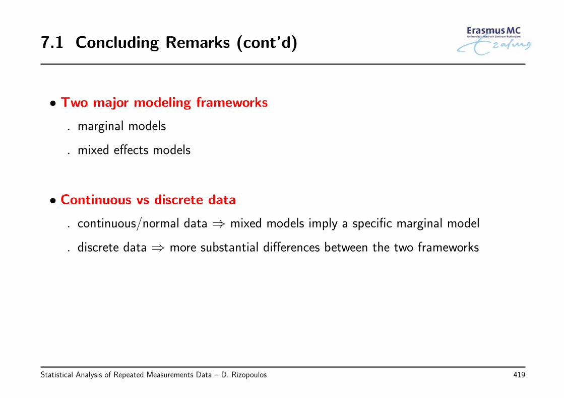
7.1 Concluding Remarks (cont’d)
• Two major modeling frameworks
◃ marginal models
◃ mixed effects models
• Continuous vs discrete data
◃ continuous/normal data ⇒ mixed models imply a specific marginal model
◃ discrete data ⇒ more substantial differences between the two frameworks
Statistical Analysis of Repeated Measurements Data – D. Rizopoulos 419
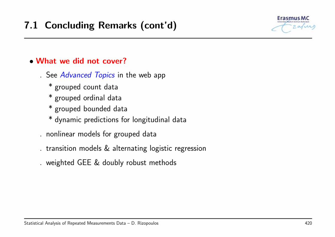
7.1 Concluding Remarks (cont’d)
• What we did not cover?
◃ See Advanced Topics in the web app
* grouped count data
* grouped ordinal data
* grouped bounded data
* dynamic predictions for longitudinal data
◃ nonlinear models for grouped data
◃ transition models & alternating logistic regression
◃ weighted GEE & doubly robust methods
Statistical Analysis of Repeated Measurements Data – D. Rizopoulos 420
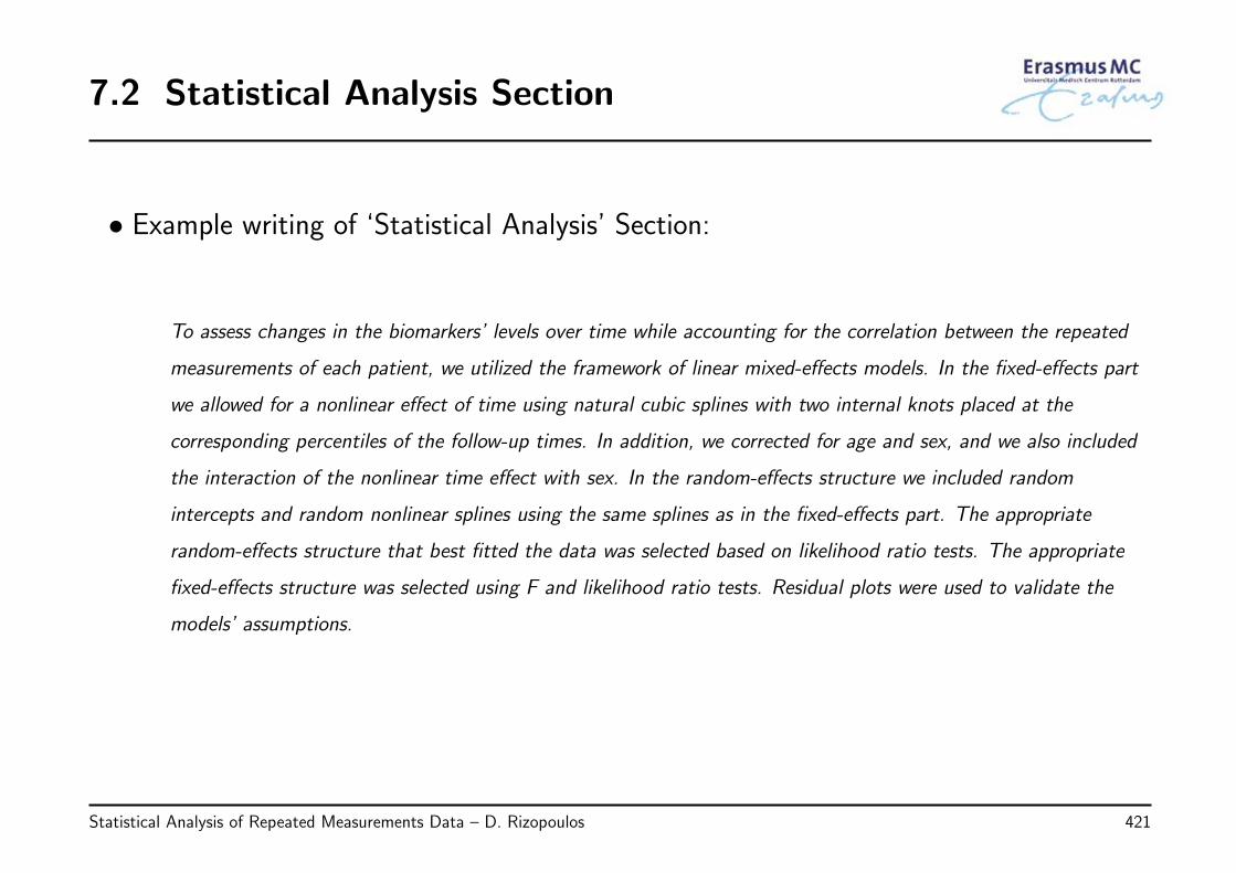
7.2 Statistical Analysis Section
• Example writing of ‘Statistical Analysis’ Section:
To assess changes in the biomarkers’ levels over time while accounting for the correlation between the repeated
measurements of each patient, we utilized the framework of linear mixed-effects models. In the fixed-effects part
we allowed for a nonlinear effect of time using natural cubic splines with two internal knots placed at the
corresponding percentiles of the follow-up times. In addition, we corrected for age and sex, and we also included
the interaction of the nonlinear time effect with sex. In the random-effects structure we included random
intercepts and random nonlinear splines using the same splines as in the fixed-effects part. The appropriate
random-effects structure that best fitted the data was selected based on likelihood ratio tests. The appropriate
fixed-effects structure was selected using F and likelihood ratio tests. Residual plots were used to validate the
models’ assumptions.
Statistical Analysis of Repeated Measurements Data – D. Rizopoulos 421

The End!
Statistical Analysis of Repeated Measurements Data – D. Rizopoulos 422
Practicals
Statistical Analysis of Repeated Measurements Data – D. Rizopoulos 423

Practical 1: Marginal Models Continuous
• We will use the PBC dataset; this is available as the object pbc2 in the R workspaceavailable on GitHub
• To load this workspace and make the data and packages available execute thefollowing steps:
1. Open a new Rstudio session
2. Create a new R script file (File → New File → R Script)
3. Copy-paste and execute the following linescon <- url("https://raw.github.com/drizopoulos/Repeated_Measurements/master/Data.RData")
load(con)
close(con)
library("lattice")
library("nlme")
library("splines")
Statistical Analysis of Repeated Measurements Data – D. Rizopoulos 424
Practical 1: Marginal Models Continuous (cont’d)
• We will need the following variables:
* id: patient id number
* prothrombin: prothrombin time in sec (the response variable of interest)
* year: follow-up times in years
* drug: the randomized treatment
* sex: the gender of the patients
* age: the age of the patients
Aim: To build an appropriate marginal model to investigate therelationships between the prothrombin time and the aforementioned
variables
Statistical Analysis of Repeated Measurements Data – D. Rizopoulos 425
Practical 1: Marginal Models Continuous (cont’d)
• Q1: We will start by producing some descriptive plots for the prothrombin time,similar to those we have seen in Chapter 1, i.e.,
◃ spaghetti plot per treatment group including the loess curve
◃ spaghetti plot per sex including the loess curve
(hint: see code for Section 1.1)
What observations can you make?
Statistical Analysis of Repeated Measurements Data – D. Rizopoulos 426
Practical 1: Marginal Models Continuous (cont’d)
• Remove outliers: From the plots you produced in Question 1 it was evident thatwe have some outlying observations
◃ for the rest of this practical we will exclude prothrombin times which were largerthan 18 sec – to do that use the following piece of code:
pbc2 <- pbc2[pbc2$prothrombin < 18, ]
Statistical Analysis of Repeated Measurements Data – D. Rizopoulos 427
Practical 1: Marginal Models Continuous (cont’d)
• We will continue by starting our model building exerciseRemember
◃ we start with a full specification of the mean structure, and investigate thecovariance structure
◃ based on our chosen covariance structure we can make inferences for the meanstructure
• Q2: Start by fitting a marginal model with independent error terms using gls() andthe following specification of the mean structure (hint: see code for Section 2.4)
◃ nonlinear time evolutions using natural cubic splines with 3 degrees of freedom
◃ correct for sex, drug and age
◃ interactions of the time effect with sex and drug
Statistical Analysis of Repeated Measurements Data – D. Rizopoulos 428
Practical 1: Marginal Models Continuous (cont’d)
• Q2:
◃ interpret the results you obtained
◃ should we simplify the model by excluding the non-significant terms?
• Q3: Continue with the same mean structure and try different covariance structures
◃ first try different correlation structures, i.e., compound symmetry, continuousAR1, linear & Gaussian, and
◃ then extend the above structures by assuming heteroscedastic errors, i.e., that thevariance increases (or decreases) over time
(hint: see code for Section 2.9)
Statistical Analysis of Repeated Measurements Data – D. Rizopoulos 429
Practical 1: Marginal Models Continuous (cont’d)
• Q4: Using appropriate tools (hypothesis tests, information criteria) decide whichstructure is the best
◃ which models are nested to which models?
• For the remainder we will use the covariance structure you have chosen in Q4
• Q5: Check if we can drop all the interaction terms
◃ with an F-test
◃ with a Likelihood Ratio Test
(hint: see code for Section 2.9)
Statistical Analysis of Repeated Measurements Data – D. Rizopoulos 430
Practical 1: Marginal Models Continuous (cont’d)
• Q6: Continue and check whether you can drop the nonlinear terms for the time effect
◃ to do that fit a model that assumes a linear time trend, and
◃ then do the likelihood ratio test to compare it to the model that includes thenonlinear terms
• Q7: Interpret the results of your final model
◃ regression coefficients
◃ covariance structure
Statistical Analysis of Repeated Measurements Data – D. Rizopoulos 431
Practical 1: Marginal Models Continuous (cont’d)
• Q8: Use an Effect Plot to depict the model with the following settings
◃ year: in the range from 0 to 12 years of follow-up
◃ sex: both males and females
◃ drug: both treatment groups
◃ age: fixed at 49 years old
(hint: see code for Section 2.4 – Effect Plot)
Statistical Analysis of Repeated Measurements Data – D. Rizopoulos 432
Practical 1: Marginal Models Continuous (cont’d)
• Q9: Check the assumptions of the model using scatterplots of the standardized &normalized residuals versus the fitted values,
◃ overall
◃ separately per sex
◃ separately per treatment group
(hint: see code for Section 2.11)
What are your conclusions?
Statistical Analysis of Repeated Measurements Data – D. Rizopoulos 433
Practical 2: Mixed Models Continuous
• We will use the PBC dataset; this is available as the object pbc2 in the R workspaceavailable on GitHub
• To load this workspace and make the data and packages available execute thefollowing steps:
1. Open a new Rstudio session
2. Create a new R script file (File → New File → R Script)
3. Copy-paste and execute the following linescon <- url("https://raw.github.com/drizopoulos/Repeated_Measurements/master/Data.RData")
load(con)
close(con)
library("lattice")
library("nlme")
library("splines")
Statistical Analysis of Repeated Measurements Data – D. Rizopoulos 434
Practical 2: Mixed Models Continuous (cont’d)
• We will need the following variables:
* id: patient id number
* prothrombin: prothrombin time in sec (the response variable of interest)
* year: follow-up times in years
* drug: the randomized treatment
* sex: the gender of the patients
* age: the age of the patients
Aim: To build an appropriate linear mixed effects model toinvestigate the relationships between the prothrombin time and the
aforementioned variables
Statistical Analysis of Repeated Measurements Data – D. Rizopoulos 435
Practical 2: Mixed Models Continuous (cont’d)
• Q1: Compute summary statistics for the number of repeated measurements perpatient
◃ do we have enough information to model potential nonlinearities in thesubject-specific trajectories?
• Q2: Examine graphically for samples of patients(hint: see code for Section 1.1)
◃ How do the individual longitudinal trajectories of the prothrombin time look like?
◃ What observations can you make?
Statistical Analysis of Repeated Measurements Data – D. Rizopoulos 436
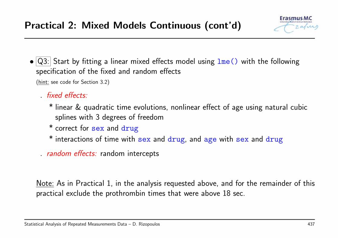
Practical 2: Mixed Models Continuous (cont’d)
• Q3: Start by fitting a linear mixed effects model using lme() with the followingspecification of the fixed and random effects(hint: see code for Section 3.2)
◃ fixed effects:
* linear & quadratic time evolutions, nonlinear effect of age using natural cubicsplines with 3 degrees of freedom
* correct for sex and drug
* interactions of time with sex and drug, and age with sex and drug
◃ random effects: random intercepts
Note: As in Practical 1, in the analysis requested above, and for the remainder of thispractical exclude the prothrombin times that were above 18 sec.
Statistical Analysis of Repeated Measurements Data – D. Rizopoulos 437
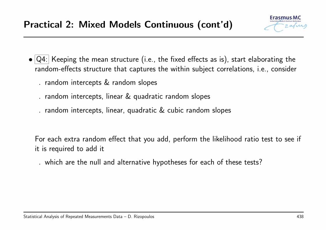
Practical 2: Mixed Models Continuous (cont’d)
• Q4: Keeping the mean structure (i.e., the fixed effects as is), start elaborating therandom-effects structure that captures the within subject correlations, i.e., consider
◃ random intercepts & random slopes
◃ random intercepts, linear & quadratic random slopes
◃ random intercepts, linear, quadratic & cubic random slopes
For each extra random effect that you add, perform the likelihood ratio test to see ifit is required to add it
◃ which are the null and alternative hypotheses for each of these tests?
Statistical Analysis of Repeated Measurements Data – D. Rizopoulos 438
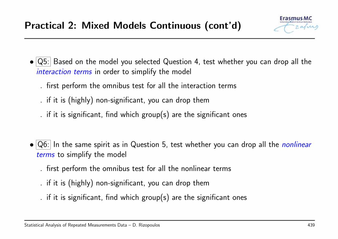
Practical 2: Mixed Models Continuous (cont’d)
• Q5: Based on the model you selected Question 4, test whether you can drop all theinteraction terms in order to simplify the model
◃ first perform the omnibus test for all the interaction terms
◃ if it is (highly) non-significant, you can drop them
◃ if it is significant, find which group(s) are the significant ones
• Q6: In the same spirit as in Question 5, test whether you can drop all the nonlinearterms to simplify the model
◃ first perform the omnibus test for all the nonlinear terms
◃ if it is (highly) non-significant, you can drop them
◃ if it is significant, find which group(s) are the significant ones
Statistical Analysis of Repeated Measurements Data – D. Rizopoulos 439
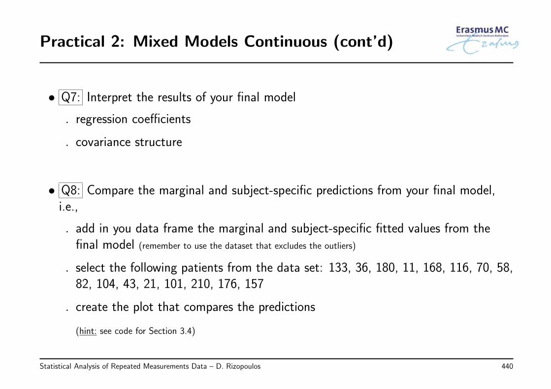
Practical 2: Mixed Models Continuous (cont’d)
• Q7: Interpret the results of your final model
◃ regression coefficients
◃ covariance structure
• Q8: Compare the marginal and subject-specific predictions from your final model,i.e.,
◃ add in you data frame the marginal and subject-specific fitted values from thefinal model (remember to use the dataset that excludes the outliers)
◃ select the following patients from the data set: 133, 36, 180, 11, 168, 116, 70, 58,82, 104, 43, 21, 101, 210, 176, 157
◃ create the plot that compares the predictions
(hint: see code for Section 3.4)
Statistical Analysis of Repeated Measurements Data – D. Rizopoulos 440
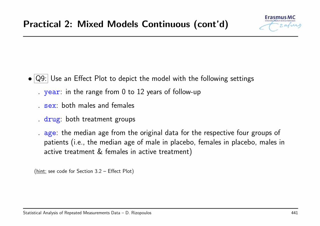
Practical 2: Mixed Models Continuous (cont’d)
• Q9: Use an Effect Plot to depict the model with the following settings
◃ year: in the range from 0 to 12 years of follow-up
◃ sex: both males and females
◃ drug: both treatment groups
◃ age: the median age from the original data for the respective four groups ofpatients (i.e., the median age of male in placebo, females in placebo, males inactive treatment & females in active treatment)
(hint: see code for Section 3.2 – Effect Plot)
Statistical Analysis of Repeated Measurements Data – D. Rizopoulos 441
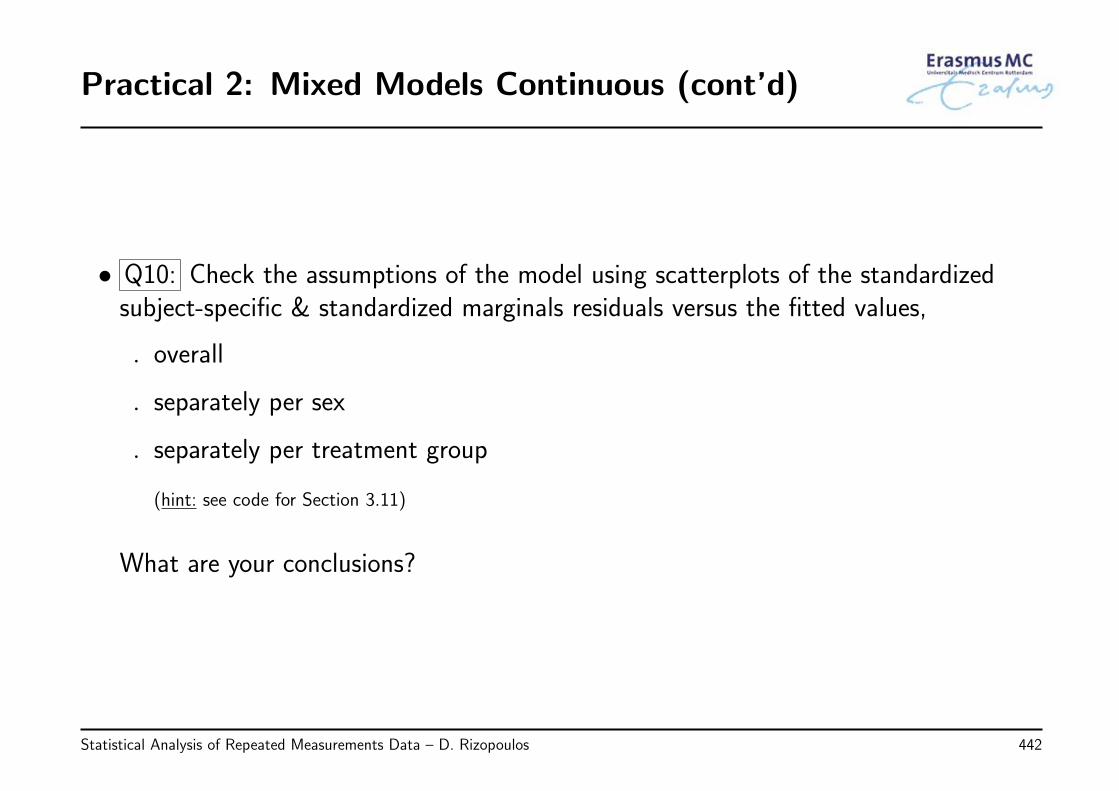
Practical 2: Mixed Models Continuous (cont’d)
• Q10: Check the assumptions of the model using scatterplots of the standardizedsubject-specific & standardized marginals residuals versus the fitted values,
◃ overall
◃ separately per sex
◃ separately per treatment group
(hint: see code for Section 3.11)
What are your conclusions?
Statistical Analysis of Repeated Measurements Data – D. Rizopoulos 442
Practical 3: Marginal Models Discrete
• We will use the PBC dataset; this is available as the object pbc2 in the R workspaceavailable on GitHub
• To load this workspace and make the data and packages available execute thefollowing steps:
1. Open a new Rstudio session
2. Create a new R script file (File → New File → R Script)
3. Copy-paste and execute the following linescon <- url("https://raw.github.com/drizopoulos/Repeated_Measurements/master/Data.RData")
load(con)
close(con)
library("lattice")
library("geepack")
library("splines")
Statistical Analysis of Repeated Measurements Data – D. Rizopoulos 443
Practical 3: Marginal Models Discrete (cont’d)
• We will need the following variables:
* id: patient id number
* prothrombin: prothrombin time in sec (the response variable of interest)
* year: follow-up times in years
* drug: the randomized treatment
* sex: the gender of the patients
* age: the age of the patients
Aim: To build an appropriate GEE model to investigate therelationships between a dichotomized version of the prothrombin
time and the aforementioned variables
Statistical Analysis of Repeated Measurements Data – D. Rizopoulos 444
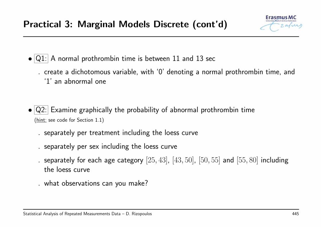
Practical 3: Marginal Models Discrete (cont’d)
• Q1: A normal prothrombin time is between 11 and 13 sec
◃ create a dichotomous variable, with ‘0’ denoting a normal prothrombin time, and‘1’ an abnormal one
• Q2: Examine graphically the probability of abnormal prothrombin time(hint: see code for Section 1.1)
◃ separately per treatment including the loess curve
◃ separately per sex including the loess curve
◃ separately for each age category [25, 43], [43, 50], [50, 55] and [55, 80] includingthe loess curve
◃ what observations can you make?
Statistical Analysis of Repeated Measurements Data – D. Rizopoulos 445
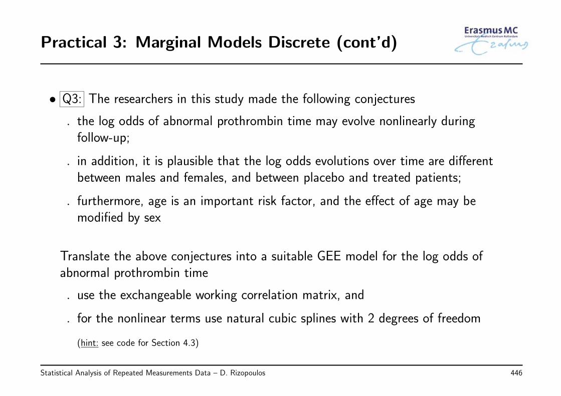
Practical 3: Marginal Models Discrete (cont’d)
• Q3: The researchers in this study made the following conjectures
◃ the log odds of abnormal prothrombin time may evolve nonlinearly duringfollow-up;
◃ in addition, it is plausible that the log odds evolutions over time are differentbetween males and females, and between placebo and treated patients;
◃ furthermore, age is an important risk factor, and the effect of age may bemodified by sex
Translate the above conjectures into a suitable GEE model for the log odds ofabnormal prothrombin time
◃ use the exchangeable working correlation matrix, and
◃ for the nonlinear terms use natural cubic splines with 2 degrees of freedom
(hint: see code for Section 4.3)
Statistical Analysis of Repeated Measurements Data – D. Rizopoulos 446
Practical 3: Marginal Models Discrete (cont’d)
• Q4: Re-fit the model you fitted in Question 3 by assuming
◃ an independence working correlation matrix, and
◃ an AR1 working correlation matrix
◃ Compare the estimated coefficients and the corresponding naive and sandwichstandard errors using a coefficients’ plot(hint: see code for Section 4.5)
◃ Which working correlation matrix do you choose and why?
Statistical Analysis of Repeated Measurements Data – D. Rizopoulos 447
Practical 3: Marginal Models Discrete (cont’d)
• Q5: The researchers in the study want to see if the model can be simplified bydropping the interaction terms
◃ first perform the omnibus test for all the interaction terms
◃ if it is (highly) non-significant, you can drop them
◃ if it is significant, find which group(s) are the significant ones
• Q6: Do the same for the nonlinear terms, i.e.,
◃ first perform the omnibus test for all the nonlinear terms
◃ if it is (highly) non-significant, you can drop them
◃ if it is significant, find which group(s) are the significant ones
Statistical Analysis of Repeated Measurements Data – D. Rizopoulos 448
Practical 3: Marginal Models Discrete (cont’d)
• Q7: Interpret the results of your final model
• Q8: Use an Effect Plot to depict the model with the following settings
◃ year: in the range from 0 to 12 years of follow-up
◃ sex: both males and females
◃ drug: both treatment groups
◃ age: 49 years old
(hint: see code for Section 4.3 – Effect Plot)
Do the plot in both the log odds and probability scales
Statistical Analysis of Repeated Measurements Data – D. Rizopoulos 449
Practical 3: Marginal Models Discrete (cont’d)
• Q9: From the effect plot we observe that the trajectories of the log odds for malesand females in the D-penicillamine group are nonlinear (more so for the females)
◃ test in males and females separately
◃ with age 49 years old
◃ whether there are differences in the log odds of abnormal prothrombin time
◃ at the follow-up years 2, 6, 8 and 10
◃ in other words, perform all the pairwise comparisons for the aforementionedfollow-up times
◃ should you adjust for multiple comparisons?
(hint: see code for Section 4.6 – complex effects)
Statistical Analysis of Repeated Measurements Data – D. Rizopoulos 450
Practical 4: Mixed Models Discrete
• We will use the PBC dataset; this is available as the object pbc2 in the R workspaceavailable on GitHub
• To load this workspace and make the data and packages available execute thefollowing steps:
1. Open a new Rstudio session
2. Create a new R script file (File → New File → R Script)
3. Copy-paste and execute the following linescon <- url("https://raw.github.com/drizopoulos/Repeated_Measurements/master/Data.RData")
load(con)
close(con)
library("lattice"); library("splines")
library("lme4"); library("GLMMadaptive"); library("MASS")
Statistical Analysis of Repeated Measurements Data – D. Rizopoulos 451
Practical 4: Mixed Models Discrete (cont’d)
• We will need the following variables:
* id: patient id number
* prothrombin: prothrombin time in sec (the response variable of interest)
* year: follow-up times in years
* drug: the randomized treatment
* sex: the gender of the patients
* age: the age of the patients
Aim: To build an appropriate GLMM to investigate therelationships between a dichotomized version of the prothrombin
time and the aforementioned variables
Statistical Analysis of Repeated Measurements Data – D. Rizopoulos 452
Practical 4: Mixed Models Discrete (cont’d)
• Q1: A normal prothrombin time is between 11 and 13 sec
◃ create a dichotomous variable, with ‘0’ denoting a normal prothrombin time, and‘1’ an abnormal one
• Q2: Examine graphically the probability of abnormal prothrombin time for eachpatient(hint: see code for Section 1.1)
◃ create the subject-specific smooth trajectories of abnormal prothrombin time forpatients who had more than five measurements
◃ use as a smoother the "splines" option in the ’type’ argument of xyplot()
◃ what observations can you make?
Statistical Analysis of Repeated Measurements Data – D. Rizopoulos 453
Practical 4: Mixed Models Discrete (cont’d)
• Q3: The researchers in this study made the following conjectures
◃ the subject-specific log odds of abnormal prothrombin time evolve linearly duringfollow-up;
◃ in addition, it is plausible that the subject-specific log odds evolutions over timeare different between males and females;
◃ furthermore, drug is expected to affect prothrombin time, and its effect may bemodified by sex
Translate the above conjectures into a suitable GLMM for the log odds of abnormalprothrombin time using random intercepts, and 15 quadrature points for the adaptiveGauss-Hermite rule(hint: see code for Section 5.2)
Statistical Analysis of Repeated Measurements Data – D. Rizopoulos 454
Practical 4: Mixed Models Discrete (cont’d)
• Q4: Test wether it is required to also include a random slopes component using alikelihood ratio test
◃ depending on the result keep the model that best fits the data
• Q5: Continue by testing whether you can drop all interaction terms from the modelusing a likelihood ratio test
• Q6: Interpret the parameters in your final selected model
Statistical Analysis of Repeated Measurements Data – D. Rizopoulos 455
Practical 4: Mixed Models Discrete (cont’d)
• Q7: Use an Effect Plot to depict the marginal log odds ratios for the followingsettings
◃ year: in the range from 0 to 12 years of follow-up
◃ sex: both males and females
◃ drug: both treatment groups
(hint: see code for Section 5.2 – Effect Plot)
• Q8: Create a second effect plot with the same settings as in Question 7 but for themarginal probabilities
◃ also include the probabilities of the median subject
Statistical Analysis of Repeated Measurements Data – D. Rizopoulos 456

No slides available for the Quizzes
Statistical Analysis of Repeated Measurements Data – D. Rizopoulos 457

No slides available for the Advanced Topics
Statistical Analysis of Repeated Measurements Data – D. Rizopoulos 458