J. Giner Navarro - CLIC WS2015 1

Statistical analysis of RF conditioning and breakdowns

Jorge GINER NAVARROCLIC Workshop 2015

26/01/2015

26/01/2015

J. Giner Navarro - CLIC WS2015 2

Overview• Introduction• Conditioning data from test stands• Magnitudes to describe conditioning status• Comparison of different structure conditionings• Conclusions

26/01/2015

J. Giner Navarro - CLIC WS2015 3

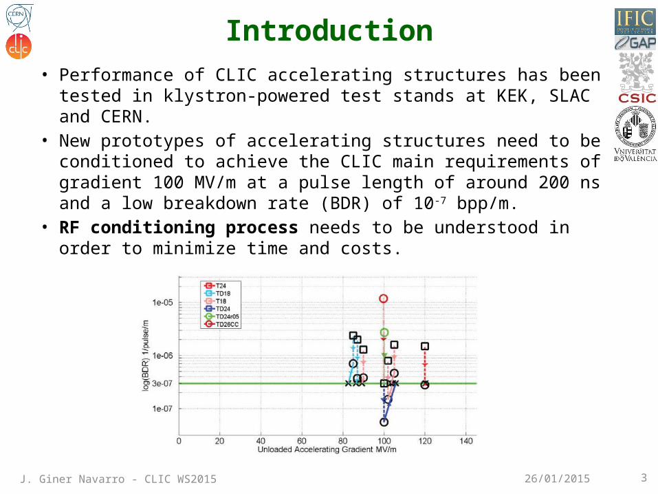
Introduction• Performance of CLIC accelerating structures has been tested in

klystron-powered test stands at KEK, SLAC and CERN.• New prototypes of accelerating structures need to be conditioned

to achieve the CLIC main requirements of gradient 100 MV/m at a pulse length of around 200 ns and a low breakdown rate (BDR) of 10-7 bpp/m.

• RF conditioning process needs to be understood in order to minimize time and costs.

26/01/2015

J. Giner Navarro - CLIC WS2015 4

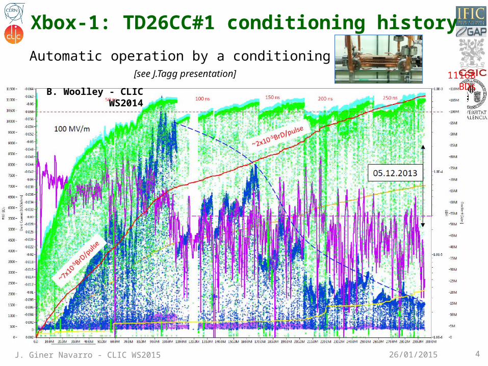
Xbox-1: TD26CC#1 conditioning historyAutomatic operation by a conditioning algorithm

[see J.Tagg presentation]

26/01/2015

11168 BDs

B. Woolley - CLIC WS2014

J. Giner Navarro - CLIC WS2015 5

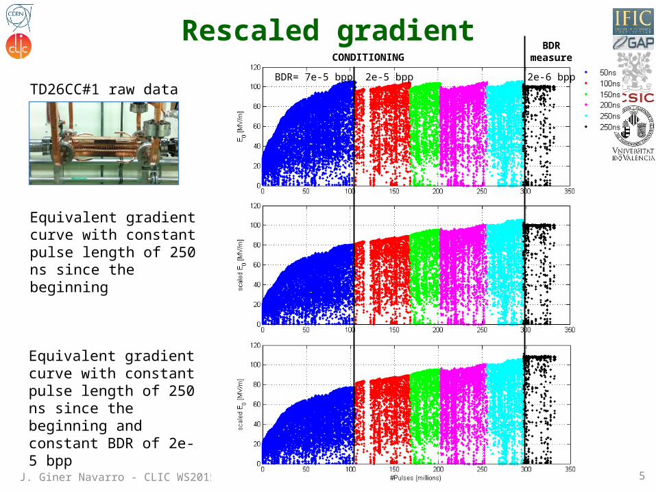
Rescaled gradient

26/01/2015

BDR= 7e-5 bpp 2e-5 bpp 2e-6 bpp

CONDITIONINGBDR

measure

TD26CC#1 raw data

Equivalent gradient curve with constant pulse length of 250 ns since the beginning

Equivalent gradient curve with constant pulse length of 250 ns since the beginning and constant BDR of 2e-5 bpp

J. Giner Navarro - CLIC WS2015 6

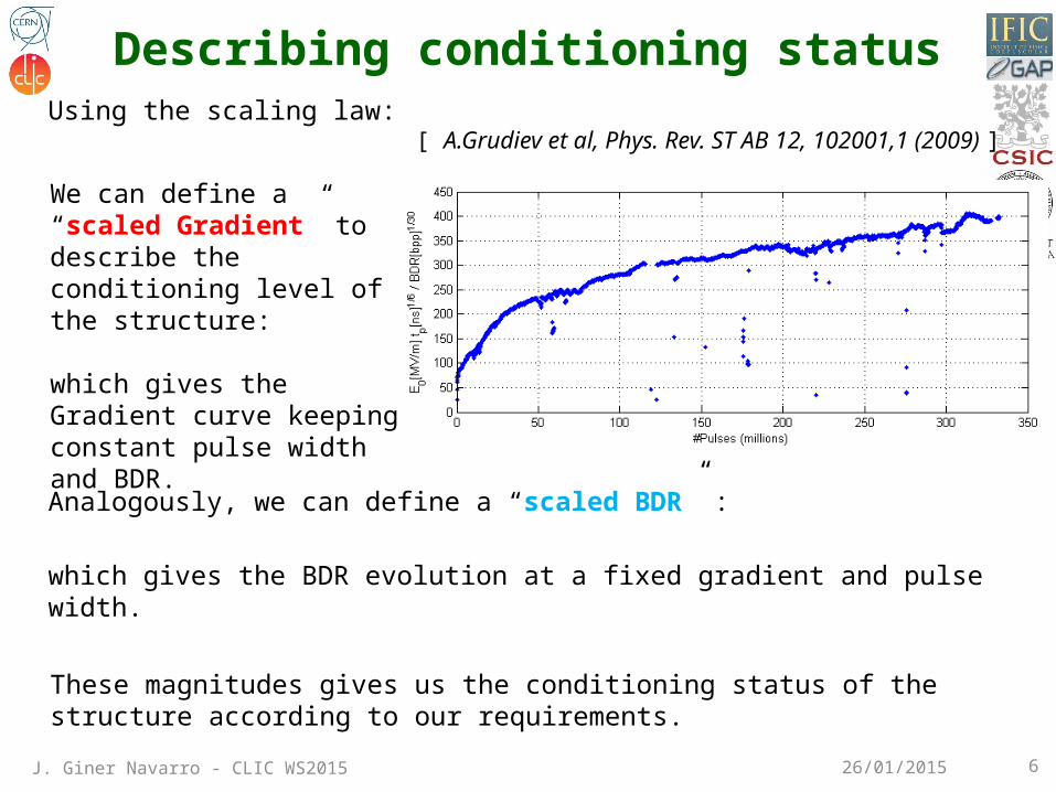
Describing conditioning status

Analogously, we can define a “scaled BDR” :

which gives the BDR evolution at a fixed gradient and pulse width.

26/01/2015

We can define a “scaled Gradient” to describe the conditioning level of the structure:

which gives the Gradient curve keeping constant pulse width and BDR.

Using the scaling law: [ A.Grudiev et al, Phys. Rev. ST AB 12, 102001,1 (2009) ]

These magnitudes gives us the conditioning status of the structure according to our requirements.

J. Giner Navarro - CLIC WS2015 7

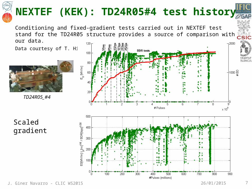
NEXTEF (KEK): TD24R05#4 test historyConditioning and fixed-gradient tests carried out in NEXTEF test stand for the TD24R05 structure provides a source of comparison with our data. Data courtesy of T. Higo.

26/01/2015

Normalized gradient here

Scaled gradient

TD24R05_#4

J. Giner Navarro - CLIC WS2015 8

Comparison of conditioning evolution

26/01/2015

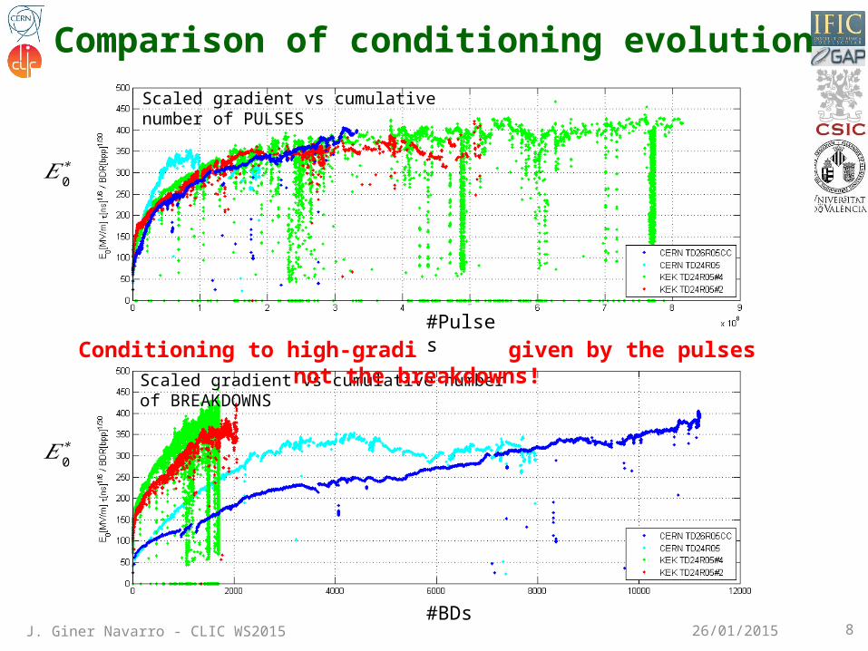
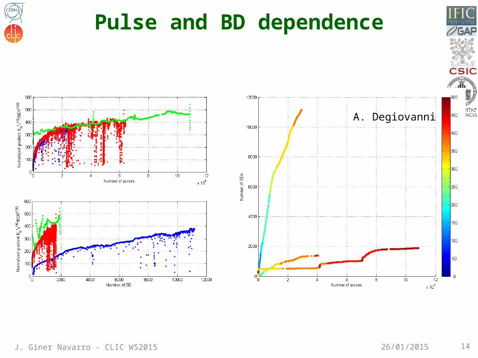
Scaled gradient vs cumulative number of PULSES

Scaled gradient vs cumulative number of BREAKDOWNS

Conditioning to high-gradient is given by the pulses not the breakdowns!

𝐸0∗

𝐸0∗

#Pulses

#BDs

J. Giner Navarro - CLIC WS2015 9

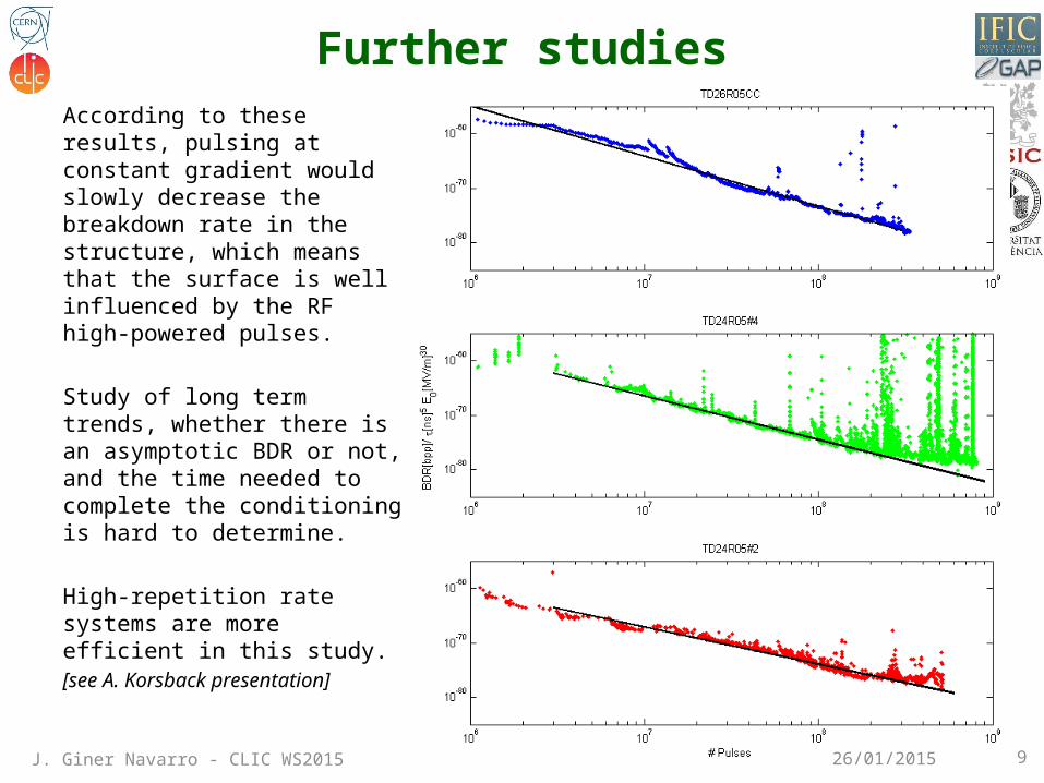
Further studiesAccording to these results, pulsing at constant gradient would slowly decrease the breakdown rate in the structure, which means that the surface is well influenced by the RF high-powered pulses.

Study of long term trends, whether there is an asymptotic BDR or not, and the time needed to complete the conditioning is hard to determine.

High-repetition rate systems are more efficient in this study.[see A. Korsback presentation]

26/01/2015

J. Giner Navarro - CLIC WS2015 10

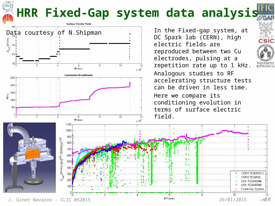
HRR Fixed-Gap system data analysis

26/01/2015

In the Fixed-gap system, at DC Spark lab (CERN), high electric fields are reproduced between two Cu electrodes, pulsing at a repetition rate up to 1 kHz. Analogous studies to RF accelerating structure tests can be driven in less time.Here we compare its conditioning evolution in terms of surface electric field.

Data courtesy of N.Shipman

J. Giner Navarro - CLIC WS2015 11

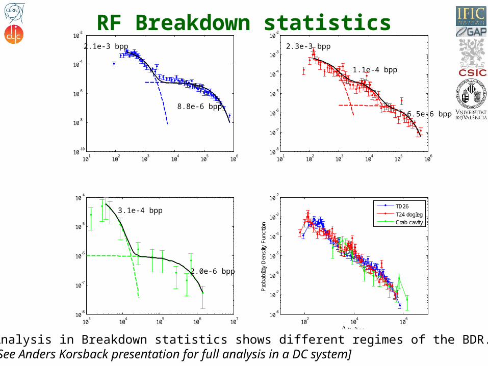
RF Breakdown statistics

26/01/201511

101

102

103

104

105

106

10-10

10-8

10-6

10-4

10-2

102

104

106

10-8

10-7

10-6

10-5

10-4

10-3

10-2

Pulses

Pro

babi

lity

Den

sity

Fun

ctio

n

101

102

103

104

105

106

10-8

10-7

10-6

10-5

10-4

10-3

10-2

103

104

105

106

107

10-8

10-7

10-6

10-5

10-4

TD26

T24 doglegCrab cavity

8.8e-6 bpp6.5e-6 bpp

2.0e-6 bpp

2.1e-3 bpp 2.3e-3 bpp

3.1e-4 bpp

1.1e-4 bpp

Analysis in Breakdown statistics shows different regimes of the BDR.[See Anders Korsback presentation for full analysis in a DC system]

J. Giner Navarro - CLIC WS2015 12

Conclusions• Working on data analysis from test stands provides a better understanding about

the conditioning process, the goal of which is the feasibility and the proper performance of the accelerating structure in the linear collider.

• Scaling laws are used to compare different structure conditionings and the same trends are found with the number of pulses, but not with the number of breakdowns.

• Different models (dislocations, local tips…) are being studied to describe the effect that the wall’s surface resists more power with increasing pulses.

• High repetition rate systems would provide valuable information in this study. The Fixed-Gap system in the DC Spark lab is running to acquire new fresh data.

• Results from this study lead to more strategies to carry out during the conditioning of the RF structure. Optimization in time (and cost) will be essential when producing new structures.

Thank you for your attention!26/01/2015

Acknowledgement to A. Degiovanni and W. Wuensch for their contribution in this work!

J. Giner Navarro - CLIC WS2015 13

EXTRA SLIDES

26/01/2015

J. Giner Navarro - CLIC WS2015 14

Pulse and BD dependence

26/01/2015

A. Degiovanni

15

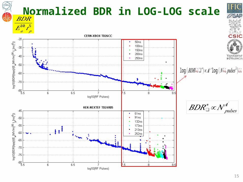
Normalized BDR in LOG-LOG scale𝐵𝐷𝑅𝐸𝑎30 𝑡𝑝

5

𝐵𝐷𝑅❑∗ ∝𝑁 𝑝𝑢𝑙𝑠𝑒𝑠

𝑨′

log (𝐵𝐷𝑅¿¿❑∗)∝ 𝑨 ′ log (𝑁¿¿𝑝𝑢𝑙𝑠𝑒𝑠❑)¿ ¿

16

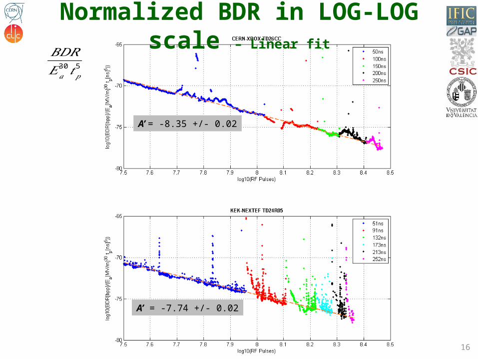
Normalized BDR in LOG-LOG scale – Linear fit

A’ = -8.35 +/- 0.02

A’ = -7.74 +/- 0.02

𝐵𝐷𝑅𝐸𝑎30 𝑡𝑝

5

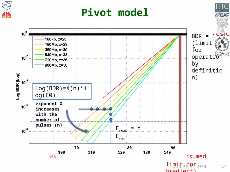
Pivot model

BDR = 1 (limit for operation by definition)

Emax (assumed limit for gradient)

The exponent X increases with the number of pulses (n)

log(BDR)=X(n)*log(E0)

Emeas = α Emax

17

70 80 90 100 110 120 130 140 155

A.D 02.04.2014

18

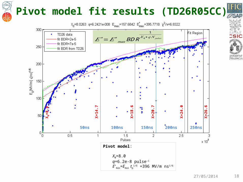
Pivot model fit results (TD26R05CC)

27/05/2014

Pivot model:

X0=8.0q=6.2e-8 pulse-1

E*max=Emax

tp1/6 =396 MV/m ns1/6

𝐸∗=𝐸∗𝑚𝑎𝑥BDR

1𝑋0+𝑞𝑁𝑝𝑢𝑙𝑠𝑒𝑠

50ns 100ns 150ns 200ns 250ns

X 0=8.

0

X=14

.7

X=18

.6

X=20

.7

X=24

.0

X=26

.6