Statistical Analysis of Spatio-temporalPoint Process Data

Peter J Diggle

Department of Medicine,

Lancaster University

and

Department of Biostatistics,

Johns Hopkins University School of Public Health

Gastroenteric disease in Hampshire, UK

Gastroenteric disease in Hampshire, UK

• 3374 incident cases, 1 August 2000 to 26 August 2001.

• largely sporadic incidence pattern

• concentration in population centres

• occasional “clusters” of cases?

Questions

• establish normal spatio-temporal pattern of reported cases(NHS Direct)

• identify spatially and temporally localised anomalies inincidence pattern (real-time surveillance)

The 2001 UK FMD epidemic

• First confirmed case 20 February 2001

• Approximately 140,000 at-risk farms in the UK(cattle and/or sheep)

• Outbreaks in 44 counties, epidemic particularly severein Cumbria and Devon

• Last confirmed case 30 September 2001

• Consequences included:

– more than 6 million animals slaughtered (4 millionfordisease control, 2 million for “welfare reasons”)

– estimated direct cost £8 billion

280000 320000 360000 400000

4600

0050

0000

5400

0058

0000

x

y

28 February

280000 320000 360000 400000

4600

0050

0000

5400

0058

0000

x

y

31 March

280000 320000 360000 400000

4600

0050

0000

5400

0058

0000

x

y

30 April

280000 320000 360000 400000

4600

0050

0000

5400

0058

0000

xy

31 May

280000 320000 360000 400000

4600

0050

0000

5400

0058

0000

x

y

30 June

280000 320000 360000 400000

4600

0050

0000

5400

0058

0000

x

y

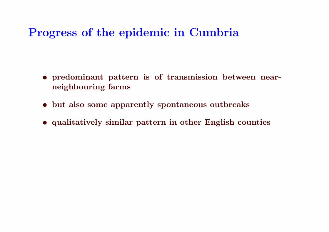
Progress of the epidemic in Cumbria

• predominant pattern is of transmission between near-neighbouring farms

• but also some apparently spontaneous outbreaks

• qualitatively similar pattern in other English counties

Questions

• What factors affected the spread of the epidemic?

• How effective were control strategies in limiting the spread?

Analysis strategies for continuous-timeprocesses

1. Empirical: log-Gaussian Cox process models – Poissonprocess with space-time intensity

Λ(x, t) = exp{S(x, t)}

2. Mechanistic: work with conditional intensity function

Ht = complete history (locations and times of events)

λ(x, t|Ht) = conditional intensity (hazard) for newevent at location x, time t, given history Ht

Analysis strategies for continuous-timeprocesses (1)

• log-Gaussian Cox process model relatively tractable(eg closed-form expressions for second-moment structure)

• also able to generate a wide range of aggregated patterns

– scientifically natural if major determinant of patternis environmental variation

– otherwise, often still a sensible empirical model

Model for gastroenteric disease data

Notation

λ0(x, t) = normal intensity of incident casesλ(x, t) = actual intensity of incident casesR(x, t) = spatio-temporal variation from normal pattern

λ(x, t) = λ0(x, t)R(x, t)

Scientific objective

• Use incident data up to time t to construct predictivedistribution for current “risk” surface, R(x, t),

• hence identify anomalies, for further investigation.

Spatio-temporal model formulation

λ(x, t) = λ0(x, t)R(x, t)

• λ0(x, t) = λ0(x)µ0(t)

• R(x, t) = exp{S(x, t)}

• S(x, t) = spatio-temporal Gaussian process:

– E[S(x, t)] = −0.5σ2

– Var{S(x, t)} = σ2

– Corr{S(x, t), S(x − u, t − v)} = ρ(u, v)

• conditional on R(x, t), incident cases form aninhomogeneous Poisson process with intensity λ(x, t)

Parameter estimation

• λ0(x) : locally adaptive kernel smootihng

• µ0(t) : Poisson log-linear regression

• σ2, ρ(u, v) : matching empirical and theoretical secondmoments (but could also use Monte Carlo MLE)

Spatial prediction

• plug-in for estimated model parameters

• MCMC to generate samples from conditionaldistribution of S(x, t) given data up to time t

• choose critical threshold value c > 1

• map empirical exceedance probabilities,

pt(x) = P (exp{S(x, t)} > c|data)

• web-reporting with daily updates

Do we need to take account of parameter uncertainty?

Spatial prediction : results for 6 March 2003

c = 2

Analysis strategies for continuous-timeprocesses (2)

Analysis via conditional intensity function

Ht = complete history (locations and times of events)

λ(x, t|Ht) = conditional intensity (hazard) for newevent at location x, time t, given history Ht

Likelihood analysis

Log-likelihood for data (xi, ti) ∈ A × [0, T ] : i = 1, ..., n,with t1 < t2 < ... < tn, is

L(θ) =n

∑

i=1

log λ(xi, ti|Hti) −

∫ T

0

∫

A

λ(x, t|Ht)dxdt

Rarely tractable, but Monte Carlo methods are becomingavailable in special cases (eg log-Gaussian Cox processes)

Partial likelihood analysis

Data (xi, ti) ∈ A × [0, T ] : i = 1, ..., n,with t1 < t2 < ... < tn

Condition on locations xi and times ti, derive log-likelihood forobserved ordering 1, 2, ..., n

• can allow for right-censored event-times if relevant

• Ri = risk-set at time ti

• pi = λ(xi, ti|Hti)/

∑

j∈Riλ(xj, ti|Hti

) (discrete Ri)

• pi = λ(xi, ti|Hti)/

∫

Riλ(xj, ti|Hti

)dx (continuous Ri)

• partial log-likelihood: Lp(θ) =∑n

i=1log pi

A model for the FMD epidemic(after Keeling et al, 2001)

Notation

• Ht = history of process up to t−

• λ(x, t|Ht) = conditional intensity

• λjk(t) = rate of transmission from farm j to farm k

Farm-specific covariates for farm i

• n1i = number of cows

• n2i = number of sheep

Transmission kernel

f(u) = exp{−(u/φ)0.5} + ρ

At-risk indicator for transmission of infection

Ijk(t) = 1 if farm k not infected and not slaughtered by timet, and farm j infected and not slaughtered by time t

Reporting delay

Simplest assumption is that reporting date is infection dateplus τ (latent period of disease plus reporting delay if any)

Resulting statistical model

λjk(t) = λ0(t)AjBkf(||xj − xk||)Ijk(t)

λ0(t) = arbitrary

Aj = (αn1j + n2j)

Bk = (βn1k + n2k)

Fitting the model

• rate of infection for farm k at time t is

λk(t) =∑

j

λjk(t)

• partial likelihood contribution from ith case is

pi = λi(ti)/∑

k

λk(ti)

FMD results

Common parameter values in Cumbria and Devon?

Likelihood ratio test: χ2

4= 2.98

Parameter estimates

(α̂, β̂, φ̂, ρ̂) = (4.92, 30.68, 0.39, 9.9 × 10−5)

But note that likelihood ratio test rejects ρ = 0.

Model extensions

• sub-linear dependence of infectivity/susceptibility on stocksize

Aj = (αnγ1j + nγ

2j)

Bk = (βnγ1k + nγ

2k)

Likelihood ratio test: χ2

1= 334.9.

• other farm-specific covariates, eg zj = area of farm j

Aj = (αnγ1j + nγ

2j) exp(z′jδ)

and similarly for Bk.

Likelihood ratio test: χ2

1= 3.26

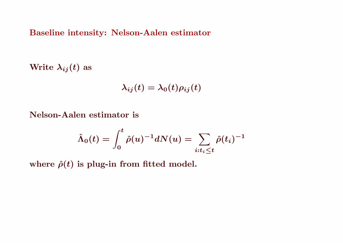
Baseline intensity: Nelson-Aalen estimator

Write λij(t) as

λij(t) = λ0(t)ρij(t)

Nelson-Aalen estimator is

Λ̂0(t) =

∫ t

0

ρ̂(u)−1dN(u) =∑

i:ti≤t

ρ̂(ti)−1

where ρ̂(t) is plug-in from fitted model.

Nelson-Aalen estimates for Cumbria (solid line)and Devon (dotted line)

50 100 150 200

0.00

00.

005

0.01

00.

015

0.02

0

time (days since 1 Feb)

cum

ulat

ive

haza

rd

An ecological application

• data record locations xi and arrival times ti of nestingbirds on several small off-shore islands

• birds known to prefer higher ground for nesting

• physical limit on distance between any two nests ≈ 25cm

• does spatio-temporal pattern of nesting sites show anyevidence of spatial interaction beyond minimumseparation distance?

Model for the pattern of nesting sites

Interaction function

h(u) =

0 : u ≤ δ0

θ : δ < u ≤ δ1 : u > δ

Conditional intensity is

λ(x, t|Ht) = λ0(t) × exp{z(x)β} × g(x, t|Ht)

• z(x) = elevation

• u∗(t) = minj:tj<t||x − xj||

• g(x, ti|Hti) = h{u∗(ti)}

Final pattern on four islands

300960 301000 301040 301080

4495

400

4495

500

Island 84

x

y

300580 300620 300660

4495

300

4495

400

Island 74

x

y

300800 300840 300880

4494

820

4494

880

4494

940

Island 61

x

y

301040 301080

4494

900

4495

000

Island 56

x

y

Confidence envelope for h(u)

Distance (meter)

exp(

thet

a)

0.0 1.5 3.0 4.5 6.0 7.5 9.0 10.5 12.5 14.5

0.0

0.5

1.0

1.5

2.0

2.5

3.0

3.5

4.0

Conclusions

• spatio-temporal point process data-sets becoming widelyavailable

• different problems require different modelling strategies

• temporal should often take precedence over spatial

• routine implementation is an important consideration