1

Statistical and technical annex to the “Report on thefunctioning of Community product and capital markets”

2

Graph 1: Price levels for private consumption - Difference with respect to the EU average (EU15=100 – Indirect taxes included) 1990-2000

Source: Eurostat/OECDNote: The figure for 2000 is an estimate. There is a break in the data series in 1992 and 1999.

40

60

80

100

120

140

160

1990 1991 1992 1993 1994 1995 1996 1997 1998 1999 2000*

A

B

D

DK

E

EL

F

FIN

I

IRL

L

NL

P

S

UK

3

Box 1

Measuring price convergence

Table 1 shows three different measures of price convergence for selected product categories. Thecalculations are based on Eurostat’s purchasing power parity data, which gives information on countriesprice level relative to the EU15-average.The first two columns show the co-efficient of variation in 1990 and in 1998. It is clear that for all but threeof the categories the price variation has decreased over this period.The next two columns measure the convergence in two different ways, each revealing how the convergencehas occurred. The first column measures convergence by computing the correlation between the initial pricelevel in 1990 and the change in the price level over the period 1990 to 1998. Converging prices will give anegative correlation between the two variables. Countries with a high price level in 1990 should havedecreasing price levels over the period; countries with a low initial price level should experience increasingprice levels. This price convergence measure is called beta-convergence. In general, the higher the beta co-efficient (in absolute value) the stronger the convergence. The measure is independent of the starting value,so a category with a very high initial price spread measured by the co-efficient of variation might have thesame beta co-efficient as a product category with a low initial price variation. For instance, “meat” and“alcoholic beverages” both show signs of strong beta-convergence, but from different initial levels.The final column measures the convergence by computing the change in the standard deviation over time.Categories for which a convergence take place will see more similar price levels and thereby a decreasingstandard deviation. For this measure the size of the co-efficient has no interpretation. The important test iswhether the sign is positive (divergence) or negative (convergence). This measure for price convergence iscalled sigma-convergence.The stars next to the co-efficient indicate whether the variables are significant at the 5 (**) or 10 (*) percentlevel, and therefore indicate for which product categories a real convergence takes place.Generally, beta-convergence is a necessary condition for convergence, but not sufficient. For example, itmight be the case that countries “switch places”, so formerly low cost countries become expensive countriesand vice-versa . This might happen without each country group’s price level getting much closer to eachother. For the category “milk, cheese and eggs” this reflects to a certain extent the case of Spain, whichinitially had a price level above the EU-average, but by 1998 had a price level below the EU-average; theopposite is true for Belgium.A sufficient condition is therefore that the standard deviation is also decreasing, which is measured by thesigma co-efficient. For the category “milk, cheese and eggs” the sigma co-efficient is negative but notsignificant indicating that although price levels in high cost countries have be decreasing and increasing inlow cost countries, there is no clear sign that the standard deviation has actually decreased in the categoryover time. On the other hand, for the category “oils and fats” there are clear signs of both sigma- and beta-convergence, indicating real convergence.All these measures are relative to the EU average. Therefore, one can not tell if convergence is taking placebecause low cost countries’ prices are rising or because high cost countries’ prices are falling.

4

Table 1

Indicators of price convergence for selected product groups (1990 - 1998)

Co-efficient of Variation Indicator 1 Indicator 2Products showing convergence 1990 1998 Beta1 Sigma2

Clothing including repairs 17% 9% -1,05 ** -0,54Oils and fats 37% 14% -0,80 ** -4,13 **Milk, cheese and eggs 14% 9% -0,75 ** -0,47Transport equipment 13% 8% -0,74 ** -1,09 **Footwear including repairs 19% 13% -0,70 ** -1,25 **Alcoholic beverages 59% 30% -0,66 ** -4,70 *Meat 26% 17% -0,66 ** -1,35 **Household textiles and repairs 25% 17% -0,61 ** -1,45 **Bread and cereals 31% 17% -0,58 ** -2,21 **Communication 35% 17% -0,57 ** -2,38 **Non-alcoholic beverages 36% 27% -0,56 ** -1,20Fruits, vegetables, potatoes 23% 16% -0,51 ** -1,04 **Personal transport equipment 26% 19% -0,41 ** -1,32 **Products not showing convergenceOperation of transport equipment 21% 17% -0,36 ** -0,34Construction 19% 23% -0,34 0,39 **Tobacco 33% 32% -0,22 -0,19Purchased transport services 26% 26% -0,15 -0,16Fuel and power 13% 18% 0,13 0,57 **Source: Eurostat PPP data from relevant years.

Note: The products are sorted first by the size of the beta estimate and secondly by whether the sigma issignificant or not. Products with a significant beta above 0,4 and a negative, significant sigma are regardedas showing convergence. A few products have a high beta but insignificant sigma. Those are regarded asshowing convergence. For the interpretation of the beta and sigma please refer to box 1.

1) The beta-co-efficients are estimated with a regression whose dependent variable is the change in Countryi's price level for good j in the relevant period. The independent variable is the initial price level for countryi and for good j. The regressions are estimated with OLS. "**" indicates that the variable is significant at the5% level. "*" indicates that the variable is significant at the 10% level.

2) The sigma-co-efficients are estimated with a regression whose dependent variable is the standarddeviation across countries for good j in year k. The independent variable is time trend. The year 1991 hasbeen dropped in the regression because there is no information for Finland in that year. "**" indicates thatthe variable is significant at the 5% level. "*" indicates that the variable is significant at the 10% level.

5

Box 2Supermarket price data

The study on supermarket prices in the EU covers all fifteen Member States minus Luxembourg. The dataset is based on electronic transaction data (bar code scanner data) from retail outlets across Europe and wascollected over a one-year period from July 1999 until June 2000. The study is carried out by AC Nielsen,UK, as part of a joint project by the Health and Consumer Protection DG, the Statistical Office and theInternal Market DG of the European Commission.The study includes price information for 68 different product categories including amongst othersaftershave, deodorants, dry and fresh pasta, frozen vegetables, mineral water, salad dressings and toothpaste.For each product, prices are reported for four different brands. A distinction is made between “PanEuropean” brands defined as brands available in more than seven Member States and “Generic” products –defined as national or multinational brands available in less than seven Member States. For each item, forinstance a certain make of toothpaste, the price of the popular size in each country and a consistent sizeacross countries is given. For certain products the popular size varies significantly across countries. Thecalculations in the annex are therefore based on weighted average prices for popular and consistent sizesusing the sales volume as weights. Results vary slightly when product categories include “Pan-European”and “generic” products or “Pan-European” products only.Yearly sales weighted average prices are reported at the national level with a regional and an outlet breakdown. The information available for each country is summarised in the table below.It should be noted that the outlet definitions vary across countries, especially for Great Britain, Ireland,Greece and the Netherlands. In addition, regional price information for Greece and the Netherlands issparse.Using scanner data collected at outlet level makes it possible to calculate average prices based on very largesamples, thereby greatly enhancing the statistical accuracy of the data. The consultant has informed theCommission that the standard error of scanner data is at least 3 times less than that for manually collectedinformation. Based on calculations for existing data, the standard error of national level data delivered to theCommission is in the range of 0,3% - 1% for small countries, and 0,2% - 0,5% for larger countries. Thestandard error for the regional and outlet data will be higher.VAT-free prices are calculated using VAT rates applicable in autumn fall 2000. The study on EUsupermarket prices is one of three studies on consumer prices. Results from two other studies on consumerelectronic goods and fresh food were reported in the Internal Market Scoreboard nr. 8, May 20011.

1 The study can be downloaded on the Internal Markets web site using the link:http://europa.eu.int/comm/internal_market/en/update/score/score8en.pdf

6

Region and outlet informationNumber of regions Outlet types

Austria 5 H,S,TBelgium 5 H,S,TDenmark 2 H,S,TFinland 6 H,S,TFrance 9 H,S,T,OGermany 7 H,S,T,D,OGreat Britain 9 S,T,OGreece 6 S,T,OIreland 4 S,T,OItaly 4 H,S,T,D,ONetherlands 5 S,TPortugal 6 H,S,T,OSpain 8 H,S,T,OSweden 6 H,S,T,OOutlet types are: Hypermarkets (H) (Size > 2500 m2), Supermarkets (S) (Size 400 – 2499 m2), Traditionals(T) (Traditional shops < 400 m2), Discounters (D) (Excluding ALDI), Others (O) (Kiosk, Pharmacies, Selfservice, Bakeries etc.)

7

Table 2 Overview of price dispersion for selected Pan-European brands

(Including taxes)

Coefficient ofVariation across

countriesMax. pricedifference

Mostexpensivecountry

Leastexpensivecountry

Average CoVacross regions

Maximum inter-regional CoV in one

country

Second largest inter-regional CoV in one

country

Nappies (Pampers baby) 9% 32% B AT 1% 3% 2%Tea (bags) (Twinnings) 12% 50% DK B 4% 12% 7%Pantyliners (Carefree) 14% 52% B Irl 2% 2% 2%Instant coffee (Nescafe) 14% 73% IT EL 2% 4% 3%Toothpaste (Colgate) 14% 65% UK P 3% 11% 7%Dry pasta (Barilla) 16% 90% B IT 3% 10% 3%Shampoo (Pantene pro) 16% 66% Irl E 2% 5% 3%Fresh pasta (Rana tortellini) 17% 62% S AT 2% 7% 3%Hair spray (Pantene) 18% 70% UK E 5% 19% 5%Ketchup (Heinz) 18% 108% IT D 2% 5% 4%Disposable razors (Bic classic) 18% 88% S D 6% 20% 9%Carbonated drinks - cola (Coca cola) 19% 90% DK D 3% 17% 4%Deodorants (Rexona) 20% 114% EL D 2% 4% 3%Face care moisturizers (Nivea) 22% 112% UK D 3% 7% 4%Toilet soaps (Dove) 23% 91% S IT 3% 5% 4%Chocolate bar (singles) (Mars) 24% 95% DK B 2% 3% 3%Carbonated drinks - cola (Pepsi) 24% 132% DK D 5% 26% 8%Salted biscuits (Tuc) 24% 89% S D 3% 6% 4%Dry pasta (Buitoni) 26% 130% B IT 4% 9% 6%Shaving foam gel (Gillette) 26% 132% Fin D 3% 8% 6%Surface cleaners (Mr Proper) 31% 161% Fin E 2% 4% 3%Surface cleaners (Ajax) 36% 281% Irl E 4% 17% 9%Mineral water (Evian) 44% 328% Fin F 3% 8% 5%Toilet soaps (Lux) 44% 194% S D 4% 6% 4%Source: DG MARKT based on AC Nielsen data

8

Table 3 Price indexes for selected product categories – EU Average = 100 (Including VAT)AT BE DK FIN FR DE GB GR IRE IT NL PT ES S

Pan European Products

Carbonated drinks – cola 90 99 139 112 78 73 113 91 92 88 116 82 93 135Carbonated drinks non cola 95 90 145 120 85 81 95 115 82 77 81 88 146Chocolate bar (singles) 98 73 143 95 85 78 98 80 106 142Disposable razors 76 129 78 93 100 84 111 89 123 103 93 121Hair conditioner 112 118 103 90 82 100 109 113 97 94 86 95Instant coffee 103 93 113 108 93 88 94 77 100 133 86 117 87 107Mineral water 116 63 189 44 85 99 76 98 58 95 176Rte cereals 123 91 88 112 94 100 71 152 115 93 85 82 93Shampoo 98 88 107 112 100 82 111 126 83 125 91 76Shaving foam gel 91 85 116 115 81 90 142 84 91 89 84 131Surface cleaners 85 83 97 129 61 107 120 71 169 64 154 44 115Toothpaste 101 94 95 88 102 126 108 109 101 101 76 76 124Generic products

Butter 102 98 127 79 99 87 102 77 124 84 98 121Drinking chocolate 78 118 91 76 56 104 147 97 76 157Flour 117 114 72 118 116 126 144 63 75 87 66Frozen pizza 103 100 103 107 99 71 110 83 89 78 152 96 108Ground Coffee and coffee beans 82 87 87 107 80 145 129 178 75 69 98 54 108Granulated sugar 106 89 113 96 120 77 114 87 100 89 110Marmalade 119 80 154 119 100 75 81 88 65 142 79 97Milk (Uht) full fat 113 65 137 121 75 133 126 64 84 78 106Milk (Uht) half fat 90 139 103 97 123 88 80 82 99Mineral water 60 79 139 153 57 109 129 73 145 49 68 39 199Washing up detergents 142 125 93 124 116 88 73 40 97 70 109 86 136Source: DG MARKT based on AC Nielsen data

9

Table 4 Price difference between Pan European Products and Generics*Number of times where “pan-

European “products are Price difference

More expensivethan “generics”

Less expensivethan “generics” Average Max Min

Aftershave 17 3 33% 171% -30%Carbonated drinks – cola 17 5 33% 153% -13%Carbonated drinks non cola 16 8 10% 44% -38%Dog food 12 3 15% 114% -41%Hair conditioner 19 3 21% 65% -15%Hair spray 14 3 28% 95% -14%Ketchup 13 3 16% 65% -10%Marmalade 9 1 18% 86% -7%Mineral water 10 1 38% 155% -11%Shampoo 16 2 39% 173% -29%Shaving foam gel 15 8 15% 64% -19%Toilet soaps 10 3 39% 137% -35%

Source: DG MARKT based on AC Nielsen data* See definitions in box 2.Note: The table is constructed by comparing – for each country for which data is available theprice of the pan-European product (usually two per product category) – with an average price ofgeneric products in the country.

Table 5 Price dispersion of homogenous versus differentiated products

HOMOGENEOUS PRODUCTSCoefficient of

variationButter 17%Chocolate flavoured milk 27%Condoms 15%Flour 30%Fresh pasta 23%Frozen vegetables 35%Granulated sugar 11%Honey 24%Milk (UHT) full fat 22%Milk (UHT) half fat 20%Milk (UHT) low fat 30%Nappies 16%Average for homogeneous products 23%Max for homogeneous products 35%Min for homogeneous products 11%

OTHER PRODUCTS (DIFFERENTIATED)Average for all other Products 31%Median for all other Products 30%Max for all other Products 68%Min for all other Products 15%

Source: DG MARKT based on AC Nielsen data

10

Graph 2 Price level for supermarket goods in the EU (EU14=100) (Prices ex VAT)

60%

70%

80%

90%

100%

110%

120%

130%

140%

150%

160%

AT BE DK FIN FR DE GB GR IRE IT NL PT ES S

Note : The graph shows the mean price level for supermarket goods (both “generic” and “pan-European” products) in different countries compared to the EU-average. In thecalculation, brands for which there is information for less then seven countries have been dropped. The graph also shows the 25 and 75 percentile price levels. The bottom ofthe vertical line indicates the 25 percentile price level, i.e. 25 percent of observations are under that price level. The top of the vertical line indicates the 75 percentile, i.e. 25percent of observations are above that price level. Consequently 50 percent of the observations can be found in the interval indicated by the vertical line.Source: DG MARKT based on AC. Nielsen data.

11

Box 3 : The Law of One Price

In an integrated market for tradable goods, competition should ensure that prices are on average more orless the same across the market. This observation is often known as the law of one price (LOOP). There aretwo versions of the law of one price. The strong version require prices to be exactly the same across themarket. The weaker version allows for regional/country specific price differences due to transport andsearch costs. These costs make price differences possible because it becomes costly for consumers andretailers to exploit price differences between different regions/countries. Each region/country can thereforehave its own price level depending on local market characteristics such as income level (wage level),storage costs, taxes, consumer preferences etc.The Commission’s price data for supermarket goods permits the testing of the LOOP both at the countrylevel and at the intra-country regional level. As national markets are more likely to be integrated, theregional results can serve as a benchmark for the law of one price.Price dispersion across countries measured by the co-efficient of variation is often in the twenties as shownin table 2. It is therefore clear that the LOOP in the strong version cannot hold for supermarket goods inEurope. The LOOP in its strong version does not seem to hold within countries either. Although the pricevariation is significantly smaller, price differences do exist between regions inside countries. The LOOPmust therefore be rejected in its strong version both at the EU and at the national level.Having rejected the strong version of the LOOP, the next step is to look at the validity of the weak version.This is done in a regression2 measuring whether there are country specific price levels across all products.This is equivalent to asking the following question for all countries: Is the price level in country X alwaysbelow/above the EU-average for all products? If the weak version of the LOOP holds, the average pricelevel in the different countries will be significantly different from the EU-average and the price variationacross countries will be mainly explained by countries. One would reject the law of one price if there issignificant difference between the price levels in the countries and country specific factors do not explain alarge part of the variation in prices across countries.The table below shows the results of a regression explaining the price variation with respect to the EUaverage by 14 country dummies3. The results confirm the existence of significant differences in the pricelevels across countries. Five countries have price levels not significantly different from the EU-average:Austria, Great Britain, Ireland, the Netherlands, and Portugal. The dummy for Greece is significant at thefive-percent level, but not at the one-percent level. For the rest of the countries, the price level deviatessignificantly from the EU-average. This would indicate that the LOOP seems not to hold for the EU.However, the estimated coefficients show large price variations across countries, and the explanatory powerof the country dummies is relatively small. Only around one fifth of the total price variation is explained bycountry specific factors. Therefore, although country specific cost factors do seem to play a role, theseresults do not seem to confirm the law of one price, even in its weak version. To check if the law of oneprice holds inside countries, a similar analysis was done for regional price levels inside countries4. Theresults are surprisingly similar to the one found for countries (see table below). Although the price variationinside countries is significantly smaller than across countries, some regions seem significantly more or lessexpensive than the country average. In addition, apart from the UK, the regional dummies seem able toexplain a similar proportion of total price variation. Generally, the weak version of the law of one price doesnot seem to hold inside countries either.

2 The ranking showed by the regression deviates from the one shown in graph 2 because the data set used isdifferent – generic products are not included in the regression because product comparability is moredifficult, which is not true of pan-European brands (Coca cola is Coca cola across the EU).3 The following equation was estimated:

εβββ ++++=

•SBEAU

i

ic DDDpp

*.....**ln 1421

pic is the price for product i in country c. pi° is the average price for product i across all countries. Onlyproducts for which there are information for more than six countries was used and only pan-Europeanbrands was included. The dummy variable DAU takes the value 1 if the country is equal to Austria and 0otherwise etc.4 To ensure comparability with the inter-country dispersion regression only prices for pan-Europeanproducts was included in the sample. In addition, products where there were missing regional informationwere dropped.

12

However, the French results seem influenced by some products with very high price variation. Droppingthese products, thereby reducing the number of products included for France from 42 to 36, significantlyincreases the explanatory power of the regional dummies in France. The unadjusted R2 increases from 0,22to 0,48. As price variation is lower in France than in other countries, this suggests that the law of one pricein its weak version does hold for France5.It is interesting to note the differences across countries. Generally, the largest intra-country price variation isfound in the UK followed by Spain, Germany and France. For these latter three there seems to be a clearregional pattern in the price differences. The explanatory power of the regional dummies is near theexplanatory power of the country dummies, with the exception of the UK. A closer look at the UK datashows exceptionally large price differences across regions for personal care items (aftershave, body careproducts, face care moisturisers, non disposable razors and toilet soap). Dropping these product slightlyimproves the explanatory power of the country-specific factors (R2 = 0,11), but does not alter the results.This analysis seems to indicate that the patterns of price differences inside countries and across countries areremarkably similar. In general, in both cases the law of one price is rejected in both versions. Moreover, asimilar amount of variation seem to be explained by regional/country patterns, with the exception of theUK. To explain price differences inside and across countries, other variables have to be introduced, forinstance the market power of producers and retailers, retail structure etc.Even though there are similarities between countries/regions, price dispersion is much higher acrosscountries. This suggests that inter-country barriers are higher than intra-country barriers.

Measuring country and regional specific effectsInter country Intra-country

Coefficients Germany Spain France UKAU -0,052 Region 1 -0,0080 * 0,00764 -0,0042 -0,0074BE -0,116** Region 2 -0,0027 -0,0125 * -0,0077** -0,0052DK 0,127** Region 3 0,0256 ** 0,0276** -0,0004 0,0075FIN 0,113** Region 4 0,0111** -0,0323** -0,0028 -0,0127 *FR -0,095** Region 5 -0,0054 -0,0015 -0,0152** 0,0090DE -0,124** Region 6 -0,0175** 0,0281** 0,0088** -0,0152**GB 0,031 Region 7 0,0047 0,0306** 0,0003 0,0074GR 0,078** Region 8 -0,0252** -0,0115 * 0,0180** -0,0045IRE 0,027 Region 9 -0,0118** -0,0030IT -0,101** Region 10 -0,0182**NL -0,027PT 0,007ES -0,191 **S 0,126 **Unadj. R2 0,216 0,21 0,19 0,22 0,04Note1: One star indicates that the variable is significant at the 10 percent level. Two stars indicate that thevariable is significant at the 5 percent level

5 The other countries also have some products with higher variation. However dropping these products fromthe regression does not significantly alter the results.

13

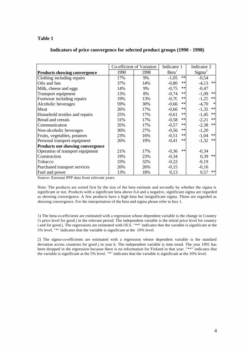
Graph 3 : Market concentration for supermarket products in different MemberStates: Average top-three firm concentration by country

0

10

20

30

40

50

60

70

80

90

AT BE DK FIN FR DE GB GR IRE IT NL PT ES S

Source: DG MARKT based on AC Nielsen dataNote: The graph shows for each country the median market share of the top 3 producers across allproduct categories. The top 3 market share is the sum of the market shares for the three biggest producersin each product category. The vertical line indicates the difference in market shares across productcategory. The bottom of the line indicates the 25 percentile market share, i.e. 25 percent of the productcategory have a concentration less than that market share. The top of the line indicates the 75 percentilemarket share, i.e. 25 percent of the product category have a concentration above that market share.Consequently, 50 percent of market shares fall in the interval indicated by the vertical line.

14

Graph 4 Price level for pan-European products (excl. VAT) and the marketshare of supermarkets

Market share of supermarkets

A T

FIN

FRES

P TIT

D

S

DK

R 2 = 0 ,4888

30%

40%

50%

60%

70%

80%

90%

6 0 70 80 9 0 100 110 1 2 0

Price level of Pan EuropeanProducts (VAT free)Source: DG MARKT based on AC Nielsen data

Note: The graph shows the price level for pan-European products excluding VAT (EU14=100) and themarket share of supermarkets. The market share of supermarkets is calculated as the total sales insupermarkets for the products in the sample compared to total sales in supermarkets, hypermarkets anddiscounters. For the definition of shop types please see box 2. Great Britain, Belgium, Ireland, theNetherlands and Greece are not shown because the data does not allow for the distinction betweenhypermarkets and supermarkets in these countries. Information on discounters is only available forGermany and Italy. The market share of supermarkets will therefore tend to be overestimated in thecalculation for the other countries.

15

Graph 5: Average price difference between hypermarkets and supermarkets forcountries with a high price level

Source : DG MARKT based on AC Nielsen data

Note : The graph shows the average price difference between hypermarkets and discounters andsupermarkets in countries with a high price level. In Austria hypermarkets are on average 4,2 percentcheaper than supermarkets. Average potential savings from buying in hypermarkets and discountersvary across countries and depending on the goods considered. It should be noted that for especiallyDenmark there is high variation in the price differences across products. Sweden, Denmark and Finlandhave the highest price levels and the highest price differences between hypermarkets and supermarkets.Austria, Italy and Portugal have lower price levels but could also benefit considerably from a morediversified distribution structure.

0%

1%

2%

3%

4%

5%

6%

7%

8%

9%

AT IT PT FIN S DK

16

Table 6A

Market indicators of integration between Internal Market and sustainabledevelopment policies

Number of ISO14000 certificates

granted

Number of ecolabelsgranted

EMAS: Number of registered sites

1997-1999Average

2000 1997-1999Average

2000 31.12.1996

31.12.1998

31.12.2000

02.10.2001

AT 123 203 n.a. n.a. 35 141 252 359BE 61 130 0 2 2 9 9 11DK 655 1 260 0 0 15 83 151 174FI 338 580 2 5 14 17 31 36FR 12 42 2 0 7 28 35 35DE 276 600 2,5 5 1116 1578 2124 2523GR 270 710 3 4 0 0 1 4IE 276 508 1 0 2 6 7 8IT 98 163 1 0 0 13 34 68LU 156 521 1 4 0 1 1 1NL 6 9 n.a. n.a. 9 19 26 27PT 336 784 1 0 0 0 1 2ES 17 47 0 0 1 18 88 151SE 450 1 370 1,7 1 15 124 183 211UK 1 019 2 534 3 0 15 59 77 78EU-15 4 092 9 461 n.a. n.a. 1231 2096 3020 3688

Sources: European Commission IX Survey on State aids, Directorate General for Taxation andCustoms Union and Internal Market Directorate General; EMAS.

17

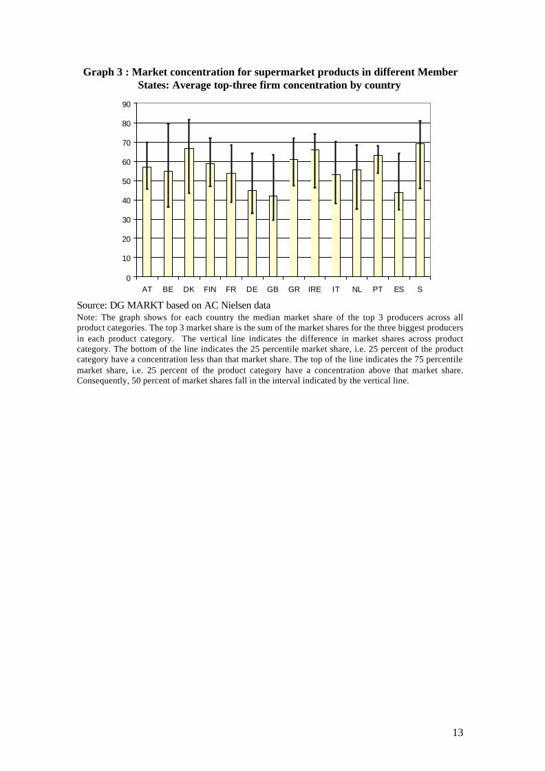
Table 6BPolicy indicators of integration between Internal Market and sustainable development policies

State aid forenvironmental and

energy savingobjectives (in mill.

euros)

Environmentalstandards notified

Internal Marketinfringements with an

environmentalcomponent

Environmentalinfringements

Transposition deficitof environmental

directives (%)

Environmentaltaxes over total tax

revenue

1996-1998Average

1999 1997-1999Average

2000 1997-1999Average

2000 1997-1999Average

2000 1997-1999Average

2000 1995-1998Average

1999

AT 55,2 57,03 4 5 1 0 18,3 29 4,5 4,3 6,4 5,2BE 5,8 5,07 4,67 1 3 3 23 19 11,7 8,6 9,3 6,2

DE 295,4 262,21 3 0 4 3 66,3 137 6,9 9,7 5,5 5,4DK 360,5 410,11 4 3 0,7 1 16 13 1,8 3,2 9,5 10,1EL 0,1 2,13 0,67 0 1,7 3 23 49 n.a. n.a. 6,5 0,7

ES 37,4 46,22 0,67 1 0,3 3 99 132 3,7 6,4 5,8 :F 54,3 78,32 3,33 1 2,3 0 65 51 6,8 6,4 9,4 :FI 31,3 63,64 1 1 n.a. n.a. 17,3 15 2,7 0 8,0 7,4

IE 2,0 5,15 0,67 0 0,3 0 43,3 110 4,8 6,4 7,7 8,0IT 57 35,3 1,33 2 3 2 39 59 5,6 3,2 9,2 9,5LU 2 2,02 0,33 0 0 0 6 7 3,3 5,4 5,2 7,3

NL 266,4 225,44 22 13 0,3 1 13,7 28 1,8 4,3 10,4 9,4PT 9,1 7,87 1,33 0 0,7 0 27,7 33 4,5 7,5 6,9 :SE 74,0 186,98 1 1 2 2 14,3 18 5 0 6,2 5,7

UK 20,1 30,9 2 5 n.a. n.a. n.a. n.a. 6,8 6,4 8,2 8,4EU15 1270,0 1418,39 n.a. n.a. 20 18 502,7 751 5,4 5,4 6,5 5,2Sources: European Commission IX Survey on State aids, Directorate General for Taxation and Custom Unions and Internal Market Directorate General.

18

Table 7Bank charges for different types of cross-border payments

BANK CARDS MANUAL EXCHANGE TRANSACTIONS

Payment by cardabroad Cash dispenser withdrawals

Cost of exchangingbanknotes in a bank

Cost of exchangingbanknotes in a “bureau de

change”

Charges, bycard-issuingcountry (€)

Charges, by card-issuingcountry

Charges by country oftransfer origin

Charge by country inwhich the withdrawal is

made

Average cost ofexchanging banknotes in a

bank

Average cost ofexchanging banknotes in a

bureau de change

Value of theoperation

(+/-) 50€ (+/-) 100€ (+/-) 50€ (+/-) 100€ (+/-) 50€ (+/-) 100€ (+/-) 50€ (+/-) 50€

A 0,38 6.73 3.89 -16% '-14% 8.88 4.8 7.14 9.77B 0,25 7.09 3.87 -10% '-8% 10.02 5.3 2.07 9.17D 0,23 10.02 5.3 37% 26% 6.77 3.87 3.01E 0 4.82 3.75 7% 0% 6.74 5.38 7.09 6.02

FIN 0 6.45 4.47 10% 3% 4.79 4.45F 0,53 7.08 3.79 56% 56% 5.65 3.43 15.09 15.76Irl 0 3.27 1.64 -6% -6% 3.91 7.04It 0 8.88 4.8 0% 0% 6.73 3.89 5.06 4.29L 0 8.6 4.96 24% 18% 9.21 8.13

NL 0,04 5.48 3.92 30% 86% 7.08 3.79 8.06 7.19P 0,32 6.74 5.38 14% -9% 4.82 3.75 2.43 5.18

Average EUR 11 0,16 6,83 4,16 +11% +8% 7,09 4,28 6,11 7,7

Source : Study by IEIC for DG SANCO, May, 2001.The results of the study represent the views of the consultant and do not represent any official position of the Commission.

19

Graph 6Retail cross-border payments: Total Credit Transfer Costs by SenderCountry and for a standards 100 euros payment (in euros)

47,24

35,99

28,47

27,87 27,3827,2 25,33

24,59 23,9222,27

21,26 21,23

14,7312,84

11,9 9,79

0

5

10

15

20

25

30

35

40

45

50

EL Ire UK P It S F E EUAv

A Fin Dk D B Nl Lux

Source: RBR. Study on the Verification of a Common and Coherent Application of Directive 97/5/EC onCross-Border Credit Transfers in the 15 Member States. Report for the Commission of the EuropeanCommunities (Internal Market Directorate General)

Graph 7Retail cross-border payments: Change in Total Credit Transfer Costs by Sender

Country (in euros): 1994 versus 2001

-44,30%

-37,70%

-23,20%

-13,70%

0,70%4,20%

11,60%

31,20% 32,70%

44,10%

-36,70%

-43,70%

-5,80%

-50%

-40%

-30%

-20%

-10%

0%

10%

20%

30%

40%

50%

B D L NL F UK EU Av DK P E IT IRL EL

Source: RBR. Study on the Verification of a Common and Coherent Application of Directive 97/5/EC onCross-Border Credit Transfers in the 15 Member States. Report for the Commission of the EuropeanCommunities (Internal Market Directorate General)

20

Graph 8 : Evolution of EU GDP vs intra-EU15 manufacturing trade(Index 1995=100)

100105110115120125130135140145150

1995 1996 1997 1998 1999 2000

Intra EU (15) trade EU GDP

Source: DG MARKT with COMEXT data.

Graph 9 : Importance of imports to Member State economies, 1995-2000

0%

10%

20%

30%

40%

50%

60%

EU

15

BLE

U

DK D EL E F Irl It

NL A P

Fin S

UK

Imports/GDP intra-EU Imports/GDP extra-EU

Source: DG MARKT with COMEXT data.

21

Graph 10 : Change in relative importance of imports by Member State1995-2000

1,80

%2,

40% 7,

10%

5,50

%

-0,5

0%1,

20% 2,

20%

3,20

%

2%

1,30

%

5,20

%1,

90%

2,80

%1,

40%

1,50

%8,

10%

0,50

%0,9

0%

1,20

%9,

80%

3,30

%3,

70%

5,90

%1,

50%

2,40

%1,

40%

1,60

%1,

90%

-1,3

0%0,

60%

-2%

-1%

0%

1%

2%

3%

4%

5%

6%

7%

8%

9%

10%

11%

12%

13%

14%

EU15 BLEU D K D EL E F Irl It N L A T P Fin S UK

In t ra-EU impor ts Impor ts f rom the res t o f the Wor ld

Source: DG MARKT with COMEXT data.

Graph 11 : The evolution of Greek manufacturing exports, 1995-2000

80

100

120

140

160

180

200

220

1995 1996 1997 1998 1999 2000

Intra-EU X Candidate countries

Source: DG MARKT with COMEXT data.

22

Graph 12 : Evolution of Foreign Direct Investment, manufacturing trade and GDPin the EU 1992-1999

0100

200300400

500600700

800900

1000

1992 1993 1994 1995 1996 1997 1998 1999

intra-EU FDI Manuf trade GDP extra-EU FDI inflows

Source: DG MARKT with COMEXT data.

Graph 13 : Importance relative to the domestic economy of Foreign DirectInvestment inflows, 1995-1999

0%

1%

2%

3%

4%

5%

6%

7%

8%

9%

EU 15 BLEU DK D EL S F Irl It NL A P F S UK

FDI inflows extra-EU FDI inflows intra-EU

Source: DG MARKT with Eurostat data.

23

Box 4

How well has the Internal Market integrated Member States’ markets?

Internal Market integration cannot continue forever. There must be a point at which integration is completeand indicators of integration show no further deepening. But what is the limit of Internal Market integrationand how close are we to hitting it? These seem reasonable questions to ask when examining the progress ofmarket integration in the EU.A simple approach to answer these questions is to ask what trade would look like in a perfectly integratedInternal Market and then to make that ideal Internal Market the benchmark with which to contrast the actualInternal Market. This is an approach used by Frankel6, for other purposes. The reasoning is as follows. In aperfectly integrated Internal Market, transport is costless, there are absolutely no barriers to trade andnobody has a preference for the goods or services of their own Member State over goods or servicesproduced in another. Assume too that this perfectly integrated internal market exists in space – i.e., there isno world beyond the EU.

Column (1) = share of EU GDPColumn (2) = intra-EU exports of goods and services / GDP

Column (3) = hypothetical intra-EU exports of goods and services / GDPColumn (4) = hypothetical exports / actual exports

1998 (1) (2) (3) (3) / (2)BLEU 3% 53% 97% 1.8Denmark 2% 20% 98% 5.0Germany 27% 14% 74% 5.4Greece 1% 18% 99% 5.6Spain 7% 17% 93% 5.4France 17% 15% 83% 5.7Ireland 1% 50% 99% 2.0Italy 14% 16% 86% 5.5Netherlands 5% 39% 96% 2.5Austria 3% 24% 98% 4.1Portugal 1% 22% 99% 4.4Finland 1% 21% 99% 4.6Sweden 3% 25% 97% 3.8United Kingdom 15% 15% 85% 5.8EU15 100% 17% 4.7

Source: DG MARKT with Eurostat data

The implication of this model ideal internal market is that the share of a Member State’s production that itsdomestic consumers consume would (on average) equal its share of total EU GDP. Take France as aconcrete example. It produced 17% of EU GDP in 1998. Therefore, if the EU were completely integrated,17% of French consumption would be on French produce, the rest would be on imports from the rest of theEU. Similarly for all other Member States. Note too, that by symmetry, if 17% of French output isdomestically consumed, the rest must be (intra-EU) exported. Using this approach, it can be calculated thatin a perfectly integrated Internal Market, intra-EU trade should be almost 5 times greater in value than it isat present (see table, final column, final row).Of course, this is not very realistic. The Internal Market will never produce such a situation, even if everybarrier to trade were eliminated. Transport costs, for example, do matter. But, nonetheless, the approach isuseful in permitting the calculation of the maximum possible impact of market integration. Also, even if itis an impossibility, movement towards that impossible degree of integration is evidence of marketintegration. Also, we can calculate the “distance” of sectors from their hypothetical benchmark in order torank sectors by their level of market integration. That can be useful for policy purposes, because sectorswhere market fragmentation seems worst and action therefore most urgent can be identified.

6 A hypothetical situation in which the proportion of products consumed in a Member State thatwere domestically produced equals that Member State’s share of EU GDP; the rest of consumption consistsof imports from EU partners. This reasoning is based on a methodology proposed J. Frankel inGlobalisation of the economy for the NBER (August 2000)

24

Box 5Measuring the benefits to be reaped from better application of the principle of mutualrecognition

Use of the model of a perfectly integrated Internal Market as described in box 5 with a minorextension can provide estimates of the maximum possible cost that failures in the principle ofmutual recognition (MRP) might be having. The extension is the assumption that a sector’s shareof industrial output is equal to that same sector’s share of intra-EU trade.MRP should apply to products where standards have not been agreed for products traded insidethe EU or to products where Member States broadly agree that national regulations can beassumed to be equivalent in effect. It is estimated that 21% of industrial production or 7% of GDPinside the EU is covered by mutual recognition7 and about 28% of intra-EU manufacturing trade8

(whose value is equivalent to about 5% of EU GDP). Assuming the internal market wereperfectly integrated9, the value of trade in products covered by mutual recognition should equaltheir contribution to GDP (i.e., 7% of EU GDP). That would imply that current trade in MRPproducts is 45% below what it would be in a perfectly integrated Internal Market, a shortfallequivalent to 1.8% of EU GDP. If, however, MRP covers 36% of intra-EU manufacturing trade10

(equivalent to just over 6% of EU GDP), then actual MRP trade is less far from what it would bein a hypothetical perfectly integrated Internal Market, although at 13% the difference is stillsignificant (equivalent to 0.7% of current EU GDP).Of course, differences between trade in a perfect internal market and today’s real internal marketare not just down to failures of mutual recognition. There are a host of other factors other thanlack of mutual recognition that cross-border trade has to overcome (e.g., language andgeography). But at least we might now know what kind of returns to enforcing mutual recognitionproperly cannot be expected. Successfully ensuring the perfect operation of mutual recognitioninside the EU tomorrow would produce a maximum possible one-off increase in EU GDP of1.8%.

7 The single market review, subseries III, volume 1: Technical barriers to trade8 op cit9 A hypothetical situation in which the proportion of products consumed in a Member State thatwere domestically produced equals that Member State’s share of EU GDP; the rest of consumption consistsof imports from EU partners. This reasoning is based on a methodology proposed J. Frankel inGlobalisation of the economy for the NBER (August 2000)10 European Commission, Cardiff Report, January 2000

25

Box 6Estimating the gains from integrating the EU’s services markets

A direct way to estimate the impact on GDP of eliminating barriers to an internal market forservices is to ask service providers for their opinion. In a survey on business services carried outfor the Commission, 40% of supply-side respondents believed that eliminating barriers to cross-border trade in business services would increase their sales (and therefore turnover) by up to 20%.Take this figure and a more conservative estimate of 5% to arrive at what might be considered aplausible range for the impact of eliminating market fragmentation on turnover in the sector.Assume that the relationship between turnover in business services and value-added is constant.Then increasing turnover 20% will also increase value-added produced by business services by20%. Now, from table 8 we can see that the contribution of business services to EU GDP is about21%. Raising turnover by 20% in business services would therefore increase EU GDP by justover 4% (20% of 21%). If, however, turnover can only be increased 5%, then the increase to EUGDP would be approximately 1%.Extrapolating from business services to all service sectors, a 20% increase in turnover wouldgenerate an increase of almost 14% in EU GDP, whilst a 5% increase in turnover would raise EUGDP by 3.4%.

26

Table 8 Comparing the service sector in the EU and the USAUSA EU

Employment GDP Employment GDPnumber

(million)Percentage billion PPS per capita percentage number

(million)percentage billion PPS per capita percentage

Total 276 7159 25.9 374 6759 18.1Labour force 136.3 170Manufacturing 21.9 16% 1475 67 21% 39.1 23% 1325 34 20%Services 101.3 74% 4968 49 69% 85.0 50% 4563 54 68%of which, business services 29.8 22% 1976 66 28% 25.5 15% 1419 56 21%Other 6.4 5% 716 112 10% 27.2 16% 872 32 13%Unemployment 6.7 5% 17.0 10%

Source: Eurostat

27

Graph 14 : Evolution of intra-EU 12 trade in construction products andmanufacturing products

100

120

140

160

180

200

220

240

1988 1989 1990 1991 1992 1993 1994 1995 1996 1997 1998 1999 2000

Construction products Manufacturing Insulating products Cement

Source: DG MARKT with COMEXT data.

Graph 15 : Home bias in investment funds: Assets invested in domestic equity fundsover total assets (December 1997- March 2001)

52,23%

47,94%

42,08%

37,82%

58,97%

44,58%

30,00%

40,00%

50,00%

60,00%

12/1

/97

3/1/

98

6/1/

98

9/1/

98

12/1

/98

3/1/

99

6/1/

99

9/1/

99

12/1

/99

3/1/

00

6/1/

00

9/1/

00

12/1

/00

3/1/

01

Source: DG MARKT with FEFSI data

28

Graph 16 : Home bias in pension funds: Assets invested in domestic equity fundsover total assets (1995-1999)

10,00

35,00

60,00

85,00

1995 1996 1997 1998 1999

B Ire P E S EU average

Source: EFRP 2001.

29

Graph 17 : Deposits held by non-residents as a % of total deposits in creditinstitutions and loans granted to non-residents as a % of total loans

granted by credit institutions (1997 and 1999)

0

10

20

30

40

50

60

AT BE DE ES FI FR IT NL PT

%

Deposits 1997 Deposits 1999 Loans 1997 Loans 1999

Source: Eurostat and ECB.

Graph 18 : Cross-border contract awards

0,0%0,2%0,4%0,6%0,8%1,0%1,2%1,4%1,6%1,8%2,0%

1995 1996 1997 1998 1999 2000

Per

cent

age

of c

ross

-bor

der

awar

ds a

s a

shar

e of

the

tota

l nu

mbe

r of a

war

ds

-

100

200

300

400

500

600

700

800

Num

ber o

f cor

ss-b

orde

r aw

ards

Cross-border tenders' number as % of total (left-hand side scale)

Number of contracts awarded to cross-border tenders (right-hand side scale)

Source: European Commission – DG MARKT – MAPP

30

Table 9 : Value of public procurement which is openly advertised/total value ofpublic procurement

1995 1996 1997 1998 1999 2000

AT 5% 8% 7% 8% 7% 13%

BE 7% 8% 11% 14% 16% 16%

DE 5% 6% 6% 7% 5% 6%

DK 16% 13% 13% 13% 14% 21%

ES 9% 11% 11% 12% 17% 25%

FI 8% 9% 8% 9% 10% 13%

FR 5% 7% 8% 11% 12% 15%

GB 15% 15% 17% 16% 15% 22%

GR 34% 37% 43% 45% 38% n.a.

IE 11% 16% 19% 16% 17% 21%

IT 10% 10% 11% 11% 13% 18%

LU 5% 7% 9% 14% 13% 12%

NL 5% 5% 6% 5% 6% 11%

PT 15% 18% 15% 16% 15% 15%

SE 12% 12% 13% 13% 14% 20%

Total EU 8% 9% 11% 11% 11% 15%

Source: European Commission, Internal Market Directorate General

31

Graph 19Total State aid over GDP and share of regional and horizontal aid (excluding rescue and

restructuring aid) over total aid (excluding agriculture and fisheries) 1995-97 and 1997-99

y-axis: Total aid over GDP (%)

0.5

0.7

0.9

1.1

1.3

1.5

1.7

1.9

2.1

2.3

20.0 40.0 60.0 80.0

1995/1997 1997/1999

Fin

P

It

NL

UK

S

E

B

F D

EULux

Dk

IrlELA

x-axis: Horizontal plus regional aid over total aid (%)

Source: IX Survey of State aids, European Commission

Box 7

The level and structure of State aid

This graph shows the evolution in the position of Member States in terms of the achievements ofthe double objective of reducing State aid spending and restructuring State aid towards lessdistortionary typess of aid (horizontal and regional aid instead of sector specific aid). It comparesthe situation of each Member State in 1995/97 and 1997/99.Countries moving towards the lower part of the graph show decreasing State aid spending. Withthe exception of Luxembourg, Ireland and the Netherlands, all Member States have reducedspending and the EU average has fallen subsequently.Countries moving towards the right-hand side of the graph have “improved” the structure of theirState aid spending by increasing the weight of horizontal and regional aid over total aid. This isthe case of Spain, Denmark, France, Belgium, Ireland, Portugal and Austria,. Moreover, onlyDenmark and to a lesser extent Austria, have lower aid spending levels and aid with lessdistortionary structure than the EU average. Given the difficulties of classifying aid by types orcategories, these results should be interpreted with caution.

32

Table 10 Comparing the distortionary effect of sector specific State aid1997-1999 (9)

Reductionbetween 1995& 1999 (as %of 1995 level)

Percentage oftotal aid in

1997

Percentage oftotal aid in

1999

Aid peremployee

(1000 euros)

Total aid overvalue of

production(%)

Total aid oversector valueadded (%)

Total aid overgross

operatingsurplus (%)

Total sectoraid overapparent

consumption(%)

Total aid overintra-EU

trade in 1999(%)

- Steel (1) 98,0 0,3 0,0 0,3 0,1 0,4 1,4 0,1 0,3- Shipbuilding (2) 53,1 1,4 1,1 6,9 5,5 17,5 199,5 7,0 16,1- Coal (3) 25,4 8,1 8,2 45,4 66,4 98,8 1.410,9 44,0 591,5- Transport (4) 17,9 33,6 40,0 13,8 18,9 34,4 (4) -Railways 12,6 31,9 39,2 25,1(4) of which Regulation1191/69

-0,6 11,4 14,0 8,8 (4)

-Airline services (5) 100,0 1,3 0,0 2,0 0,6 0,3 (4)- Tourism (6) -43,9 0,4 0,5 0,2 0,2 0,5- Financial services (7) 4,9 3,6 1,4 1,1- Media and culture -10,5 1,0 0,9- Motor vehicles (8) 71,2 0,3 0,1 0,1 0,1 0,2 0,9 0,1 0,1(1) (NACE rev 1 27.1 27.2 & 27.3) Data not available for Irl and Nl in all categories, and for L, A, and Dk for "other iron and steel products". 1996 data for EL and F (for "basic iron and steel"), EL, I and L (for"tubes") and EL and I for "other".(2) (NACE Rev. 1 35.1) data not available for Nl.(3) (NACE Rev. 1 10.1 .2 .3) For peat, there is not data available for the UK, A, NL, Irl, E, Dk and B and for lignite there is no data for the UK, A, E and EL. For hard coal, production value in F has been estimatedon the basis of physical output and there is no data for value added and operating surplus.(4) (NACE rev 1.60, 61 & 62) Production does not include Bleu, D, El and UK and Value added does not include D and EL. Employment does not include EL and UK.1998 data for E and 1996 for I. Data for Dkinclude Nace rev 1 62 only and for Fin Nace rev 1 61 & 62 only.(5) (Nace Rev 1 62) Data not available for D, NL, L and EL. 1996 for I Fin & S. For employment, data do not include the UK, S, NL, L and EL and 1996 data for I & Fin.(6) (NACE Rev 1 55.1-5 and 63.3) Incomplete data for 55 (UK, D, S, Irl, E, EL & Dk) and for 63 (DK, D, EL, S, UK and L). 1996 data for I.(7) Lower bound estimate ; incomplete for "insurance" and "financial houses".(8) (NACE Rev. 1 35.1) Data not available for A, L and Nl (employment only). 1996 data for I and Gr. Aid does not include cases below the notification ceilings.(9) Production, value added, trade and employment figures for 1997. Average for 1997-1999 for aid values.

Source: Eurostat SBS, Panorama of the European Industry and IX Survey of State aids, European Commission.

33

Box 8Comparing the distortionary effects of sector-specific State aid

Last year’s Internal Market Council conclusions insisted on the need to have a more in-depth insight of the reallydistortionary impact of different forms of State aid. The distortionary impact of aid can only be measured case bycase and is market specific. Overall conclusions based on aggregated information can be misleading. However,industry specific information for the EU 15 can be used to calculate some indicators that give us a very rough butstill approximate idea about the relative impact of sector-specific aid in sectors where aid is significant.Using aid as a percentage of value added, intra EU trade and employment as indirect indicators of thedistortionary impact of State aid in these industries, it becomes apparent that aid to coal has a particularlydistortionary impact on normal competition conditions in this market. This conclusion is reinforced by two facts:aid to coal is granted in four countries only and a substantial proportion of the total aid is granted to coveroperational costs. Special reasons of security of energy supply and the social impact of aid in this sector oncertain regions explain this situation. Nonetheless, while the social and regional functions of these aidprogrammes have been recognised, their cost-effectiveness has progressively been put into question. MemberStates have taken steps to diminish coal aid by price support, instead maintaining regional assistance by other lessdistortionary means. The Commission has also presented a draft regulation for aid to the coal sectorencompassing these social and security of supply goals combined with a steady and significant reduction of aidlevels to put an end to this situation. This regulation is to replace existing rules on expiry of the ECSC Treaty inJuly 2002.The second sector where the risk of significant market distortion is high is transport. Most aid in this sector goesto railways but a significant percentage of that aid is compensation for public service obligations, and the sector isunder strict State aid guidelines. In air transport, there has been a drastic reduction in the volume of aid in the lastfive years. The Commission has indicated that it is prepared to authorise certain limited, temporary measures toavert the damages directly caused by the exceptional events of September 11, although it does not believe thatstate aid is the appropriate response to a decline in demand.. Aid to shipbuilding and steel has decreased involume but is still high, especially in shipbuilding. It is worth mentioning the increasing level of State aid forsectors such as media, culture and tourism. Although levels are still low, attention should be paid to their futureevolution.

34

Graph 20 : Total State aid by type 1995-1999 (excluding agriculture and fisheries)

(in millions of 1998 euros)

Hor izonta l

Sector specific

Regional

0

10000

20000

30000

40000

50000

60000

70000

80000

90000

1995 1996 1997 1998 1999

Hor izonta l Sector specif ic Regiona l

Source : IX survey of State Aids, European Commission

35

Box 9State aid and the Lisbon objectives

The Lisbon European Council defined overall objectives for transforming Europe into the world’s mostcompetitive economy. Grouped under four broad categories: innovation, employment, economic reform andcohesion, the Gothenburg European Council added a fifth category: sustainable development. State aids areneither the only nor the main instrument to attain those five objectives, but they can be more or less orientedtowards achievement of the Lisbon objectives.Graph A below shows that aid which may be considered as not contributing to the Lisbon objectives (even if weinclude all aid to SMEs and the extended Lisbon objectives after Gothenburg) presents a clear upward trendbetween 1995 and 1999. Graph B shows that in 1999 only Portugal, thanks to cohesion aid, and Denmark, with itsmore balanced composition of State aid, was over 40% of aid aiming to comply with the Lisbon objectives. Onceagain, these conclusions should be interpreted with caution because it is difficult to establish a precisecorrespondence between aid categories and the Lisbon objectives.

Graph A : EU 15: Aid not contributing to the Lisbon objectives 1995 - 1999 over total aid(excluding agriculture and fisheries)

1995 1996 1997 1998 1999

64,00

66,00

68,00

70,00

72,00

74,00

76,00

78,00

80,00

82,00

84,00

Excluding aid for Lisbon obj. from total aid

Excluding aid for Lisbon obj. + environment from total aid

Excluding aid for Lisbon obj. + environment + SME from total aid

%

Source: IX Survey of State aids, European Commission

36

Graph B: Aid for "Lisbon objectives" over total aid (excluding agriculture and fisheries) 1999

0%

20%

40%

60%

80%

100%

A B DK D E L E FIN IRL IT L NL P S UK

Non-Lisbon objectives Cohesion Employment-training Innovation Environment/Energy SMEs

Source: IX Survey of State aids, European Commission

37

Table 11 : Effective Average Tax Rate by country by asset, source of finance and overall -1999& 2001

(Corporation taxes only)

EFFECTIVE AVERAGE TAX RATES1999 1999

Cou

ntry

Cor

pora

teta

x ra

tes

(1) 2

001

Ove

rall

Mea

n20

01

Cor

pora

teta

x ra

tes

(1) 1

999

Ove

rall

Mea

n 19

99

Inta

ngib

les

Indu

stri

alB

uild

ings

Mac

hine

ry

Fina

ncia

lA

sset

s

Inve

ntor

ies

Ret

aine

dea

rnin

gs

New

equ

ity

Deb

t

AU 34.00 27.9 34.00 29.8 28.6 29.2 28.4 33.2 29.9 33.9 33.9 22.3B 40.17 34.5 40.17 34.5 30.7 36.1 31.0 39.2 35.3 39.1 39.1 25.8D 39.35 34.9 52.35 39.1 33.9 39.0 34.9 46.8 40.8 46.1 40.1 27.7Dk 30.00 27.3 32.00 28.8 21.3 34.7 25.3 31.2 31.2 32.3 32.3 22.1E 35.00 31.0 35.00 31.0 31.1 31.8 27.4 34.2 30.7 35.2 35.2 23.3EL 37.50 28.0 40.00 29.6 35.5 30.4 33.4 11.6 37.1 34.4 34.4 20.8F 36.43 34.7 40.00 37.5 30.6 40.6 40.1 39.0 37.1 42.1 42.1 28.8Fin 29.00 26.6 28.00 25.5 24.8 24.8 23.1 27.3 27.3 28.8 28.8 19.3It 40.25 27.6 41.25 29.8 24.9 29.8 27.4 36.1 31.1 31.8 31.8 26.1Ire 10.00 10.5 10.00 10.5 8.9 15.8 8.2 9.8 9.8 11.7 11.7 8.2Lux 37.45 32.2 37.45 32.2 28.6 33.7 29.2 36.6 32.9 36.6 36.6 24.0NL 35.00 31.0 35.00 31.0 26.7 32.4 29.2 34.2 32.5 35.1 35.1 23.3P 35.20 37.0 37.40 32.6 33.2 31.8 28.6 36.5 32.8 37.0 37.0 24.5S 28.00 22.9 28.00 22.9 19.6 23.4 19.7 25.7 25.7 26.0 26.0 17.1UK 30.00 28.3 30.00 28.2 24.2 33.7 24.7 29.3 29.3 31.8 31.8 21.6

Source : Company taxation in the Internal Market, (SEC(2001)1681)Note. Each asset column represents an average across all three types of finance, with weights of 55% retained earnings,10% new equity and 35% debt. Each finance column represents an un-weighted average across all 5 assets. The overallaverage is an average across all 15 types of investment, with the same weights.(1) Including surcharges and local taxes

38

Box 10

Start-up costs in time and money

A key element for entrepreneurship and competition is easy market entry. Entry conditions are heavilydependent on the set-up costs of the new firm as well as the administrative procedures that starting-up anew business entails. For new entrepreneurs not only money matters. Time spent on the administrativeprocess of setting-up a company extends the very difficult period until it reaches its break-even point andstarts to make profit. This is especially true for one-man enterprises.Measuring entry conditions is not an easy task. Entry conditions (time, cost, administrative complexity)depend inter alia on the legal form, economic sector and geographic location of the firm. In addition, legalforms vary across countries, making comparisons more difficult. Finally, we can measure average orminimum time, costs and administrative procedures.The recent entrepreneurship scoreboard has presented data on the minimum time and costs for setting upindividual enterprises and private limited companies in the EU (see table A). The term ‘minimum’ refersto the least time (or cost) that could be involved in setting up the enterprise, given the current regulations.It is more an indicator of regulatory complexity than of administrative efficiency. Early next year theCommission will also produce data that attempts to indicate the 'typical' time that it takes to set up anenterprise. Here, the element of administrative efficiency will also come into the picture.A recent Austrian study has produced figures of “standard” cost, time and number of administrativeprocedures for start-ups in some EU Member States and other countries (see table B). A simplecomparison of the figures in these two tables makes apparent the high sensitivity of the results to themethodology used for benchmarking start-up costs. But leaving aside differences in methodologies, theresults of both studies show huge differences across countries in the costs and time necessary to start anew business. However, most Member States have shortened the administrative processes and costs inrecent years. Countries like Denmark might be seen as best practices by other Member States where suchprocedures are still expensive and time consuming.

Table A: Minimum time and costs for setting up individual enterprises and privatelimited companies

Minimum Costs (€) Minimum Time (days)IndividualEnterprise

Private LimitedCompany

IndividualEnterprise

Private LimitedCompany

AU 0 1120 1 10B 62 980 2 16Dk 0 0 6 7F 50 213 3 4Fin 58 252 7 7D 15 634 1 3ELe 750 1700 2 3It 25 1270 2 4Ire 32 445 6 7Lux 150 850 15 25NL 45 535 1 5P 10 450 6 13En 0 1518 2 11S 88 186 6 8UK 0 40 1 3EU* 85,7 679,5 4,1 8,4* unweighted averageSource: DG Enterprise, 2001.

39

Table B:Process of setting-up of a firm

A D SWE NL FIN DK* IRL* NOR* NZL* CAN* USA*Number of stepsSole proprietorships 6 5 2 6 3Limited partnership 8 7 2 7 3Limited liability company 9 8 3 7 6 3 3 4 3 2 3DurationSole proprietorships 3 4 11 6 33Limited partnership 23 15 20 7 33Limited liability company 25 16 22 34 35 2 11 2 1 2 2Costs in €Sole proprietorships 0 0 0 66 59Limited partnership 785 798 88 111 118Limited liability company 1.730 2.203 188 1.949 252 3.612 2.499 1.750 82 315 171* Data for limited liability companies: Worldbank country files.Source: Lettmayr, C. F. / Mandl, I. / Gruber, E. (2001): Gründungskosten neuer Unternehmen in Österreich und Policy-Benchmarking im Bereich der Unternehmensgründung. Vienna: Austrian Institute for Small Business Research.

Graph 21 :Evolution of Risk capital in the EU (millions €)

55465813

4214

6693

7960

20002 20343

463241264271 41155440

6788

9655

14461

25116

34610

47014579 4188 3425

4398

48023

25401

0

5000

10000

15000

20000

25000

30000

35000

40000

45000

50000

89 90 91 92 93 94 95 96 97 98 99 00

Annual Investment Funds raised 3-year mov. Avrg., Investments 3-year mov. Avrg., Funds raised

Source: EVCA, Annual survey of private equity and venture capital in Europe

40

Table 12:

European Venture Capital Investment Trends, 1996-2000 (in thousand euros)

1996 1998 2000Amount % Amount % Amount %

Stage distribution:Seed 68,992 1.0 169,271 1.2 819,680 2.3Start-up 375,430 5.5 1,468,511 10.2 5,843,723 16.7Expansion 2,712,015 40.0 4,334,539 30.0 12,986,306 37.1Replacement Capital 481,014 7.1 1,078,675 7.5 930,092 2.7Buyout 3,150,195 46.4 7,409,785 51.2 14,405,952 41.2Total Investment 6,787,646 100 14,460,781 100 34,985,752 100

Sectoral distribution:Bio-technology 182,355 2.7 346,354 2.4 1,017,185 2.9High-tech Investment 1,347,926 19.9 4,026,917 27.8 10,976,494 31.4Source: EVCA, 2001.

41

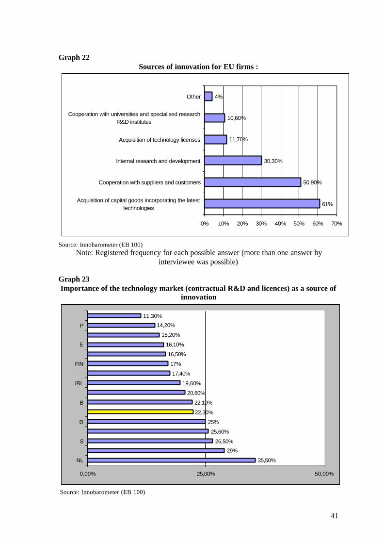
Graph 22Sources of innovation for EU firms :

61%

50,90%

30,30%

11,70%

10,60%

4%

0% 10% 20% 30% 40% 50% 60% 70%

Acquisition of capital goods incorporating the latesttechnologies

Cooperation with suppliers and customers

Internal research and development

Acquisition of technology licenses

Cooperation with universities and specialised researchR&D institutes

Other

Source: Innobarometer (EB 100)Note: Registered frequency for each possible answer (more than one answer by

interviewee was possible)

Graph 23Importance of the technology market (contractual R&D and licences) as a source of

innovation

35,50%

29%

26,50%

25,60%

25%

22,30%

22,10%

20,60%

19,60%

17,40%

17%

16,50%

16,10%

15,20%

14,20%

11,30%

0,00% 25,00% 50,00%

NL

S

D

B

IRL

FIN

E

P

Source: Innobarometer (EB 100)

42

Table 13:Preferred strategy for the protection of industrial and intellectual property rights in

EU countriesCountry Keeping the

innovationsecret and

benefit fromtime advantage

Trade marks,industrial models

or designsPatents No answer or other

EL 32,60% 43,80% 15,70% 7,90%P 38,40% 27,90% 17,40% 16,30%

DK 53,20% 20,70% 8,50% 17,60%E 56,60% 17,40% 15,30% 10,70%

AT 59,20% 14,50% 15,60% 10,60%B 59,40% 17,60% 12,70% 10,30%

UK 59,40% 15,30% 10,10% 15,30%NL 60,80% 19,90% 12,20% 7,20%F 61,10% 13,80% 14,80% 10,40%

EU 15 63,30% 14,30% 13,90% 8,50%SW 63,40% 14% 11,60% 11%FIN 65,30% 22,10% 6,30% 6,30%D 66,70% 12,10% 17% 4,30%L 67,10% 11,80% 16,50% 4,70%

IRL 73,30% 14,40% 11,10% 1,10%IT 73,50% 8,40% 10,40% 7,80%

Source: Innobarometer (EB 100)