Statistical Applications in Genetics and Molecular Biologycmatias.perso.math.cnrs.fr/Docs/SAGMB_Arribas_Matias.pdf · Volume 11, Issue 1 2012 Article 5 Statistical Applications in

Volume 11, Issue 1 2012 Article 5

Statistical Applications in Geneticsand Molecular Biology

A Context Dependent Pair Hidden MarkovModel for Statistical Alignment

Ana Arribas-Gil, Universidad Carlos III de MadridCatherine Matias, Laboratoire Statistique et Génome,

Université d'Évry Val d'Essonne, UMR CNRS 8071, USCINRA

Recommended Citation:Arribas-Gil, Ana and Matias, Catherine (2012) "A Context Dependent Pair Hidden MarkovModel for Statistical Alignment," Statistical Applications in Genetics and Molecular Biology:Vol. 11: Iss. 1, Article 5.DOI: 10.2202/1544-6115.1733

©2012 De Gruyter. All rights reserved.Brought to you by | Cambridge University Library

AuthenticatedDownload Date | 12/15/16 7:17 PM

A Context Dependent Pair Hidden MarkovModel for Statistical Alignment

Ana Arribas-Gil and Catherine Matias

AbstractThis article proposes a novel approach to statistical alignment of nucleotide sequences by

introducing a context dependent structure on the substitution process in the underlying evolutionarymodel. We propose to estimate alignments and context dependent mutation rates relying on theobservation of two homologous sequences. The procedure is based on a generalized pair-hiddenMarkov structure, where conditional on the alignment path, the nucleotide sequences followa Markov distribution. We use a stochastic approximation expectation maximization (saem)algorithm to give accurate estimators of parameters and alignments. We provide results both onsimulated data and vertebrate genomes, which are known to have a high mutation rate from CGdinucleotide. In particular, we establish that the method improves the accuracy of the alignment ofa human pseudogene and its functional gene.

KEYWORDS: comparative genomics, contextual alignment, DNA sequence alignment, emalgorithm, insertion deletion model, pair hidden Markov model, probabilistic alignment, sequenceevolution, statistical alignment, stochastic expectation maximization algorithm

Author Notes: The work of A. Arribas-Gil was partially funded by the Spanish Ministry of Scienceand Innovation (ECO2008-05080, HI2008-0069, “José Castillejo” grant JC2010-0057) and Regionof Madrid, Spain (CCG10-UC3M/HUM-5114). Also, part of this work was carried out during visitsof A. Arribas-Gil to the Department of Statistics at the University of California, Davis, and toCNRS “Laboratoire Statistique et Génome.”

Brought to you by | Cambridge University LibraryAuthenticated

Download Date | 12/15/16 7:17 PM

1 IntroductionAlignment of DNA sequences is the core process in comparative genomics. An

alignment is a mapping of the nucleotides in one sequence onto the nucleotides

in the other sequence which captures two important evolutionary processes: the

substitution (of a nucleotide, by another one) and the insertion or deletion (indel,

of one or several nucleotides). Thus, in this mapping, two matched nucleotides

are supposed to derive from a common ancestor (they are homologous) and the

mapping also allows for gaps which may be introduced into one or the other se-

quence. Several powerful alignment algorithms have been developed to align two

or more sequences, a vast majority of them relying on dynamic programming meth-

ods that optimize an alignment score function. While score-based alignment proce-

dures appear to be very rapid (an important point regarding the current sizes of the

databases), they have at least two major flaws: i) The choice of the score param-

eters requires some biological expertise and is non objective. This is particularly

problematic since the resulting alignments are not robust to this choice (Dewey,

Huggins, Woods, Sturmfels, and Pachter, 2006). ii) The highest scoring alignment

might not be the most relevant from a biological point of view. One should then

examine the k-highest scoring alignments (with the additional issue of selecting a

value for k) but this approach often proves impractical because of the sheer num-

ber of suboptimal alignments (Waterman and Eggert, 1987). We refer to Chapters 2

and 4 in Durbin, Eddy, Krogh, and Mitchison (1998) for an introduction to sequence

alignment.

Contrarily to score-based alignment procedures, statistical (or probabilistic)

alignment methods rely on an explicit modeling of the two evolutionary processes

at the core of an alignment, namely the substitution and the indel processes. While

there is a general agreement that substitution events are satisfactorily modeled re-

lying on continuous time Markov processes on the nucleotide state space, very few

indel models have been proposed in the literature and none of them has become a

standard. The first evolutionary model for biological sequences dealing with indels

was formulated by Thorne, Kishino, and Felsenstein (1991), hereafter the TKF91

model. It provides a basis for performing alignment within a statistical framework:

the optimal alignment is obtained as the evolutionary path that maximizes the like-

lihood of observing the sequences as being derived from a common ancestor (under

this model). This has at least two major advantages over the score-based method.

First, in this context, the evolutionary parameters (which play the role of an under-

lying scoring function) are not chosen by the user but rather estimated from the data,

in a maximum likelihood framework. Second, a posterior probability is obtained on

the set of alignments: the analysis does not concentrate on the highest probable path

but rather provides sample alignments from this posterior distribution. Moreover,

1

Arribas-Gil and Matias: Context Dependent Statistical Alignment

Published by De Gruyter, 2012



´ ´

´

´

¨

a confidence measure may be assigned to each position in the alignment. This is

particularly relevant as alignment uncertainty is known to be a major flaw in com-

parative genomics (Wong, Suchard, and Huelsenbeck, 2008).

Statistical alignment of two sequences is performed under the convenient

pair-hidden Markov model, hereafter pair-HMM (see Arribas-Gil, Gassiat, and

Matias, 2006, Durbin et al., 1998), enabling the use of generalizations of the ex-

pectation-maximization (em) algorithm (Dempster, Laird, and Rubin, 1977). Some

drawbacks of the preliminary TKF91 proposal have been improved by these au-

thors in what is called the TKF92 version of the model (Thorne, Kishino, and

Felsenstein, 1992). Then, the original models later have been refined in many

ways, as for instance in Arribas-Gil, Metzler, and Plouhinec (2009), Knudsen and

Miyamoto (2003), Metzler (2003), Miklos (2003), Miklos, Lunter, and Holmes

(2004), Miklos and Toroczkai (2001). We underline that an important characteristic

of all those models is that the indel and the substitution processes are handled inde-

pendently. An introduction to statistical alignment may be found in Lunter, Drum-

mond, Miklos, and Hein (2005). Note that we will be dealing with the alignment of

two sequences only, which has itself its own interest. However, our approach could

be seen as a first stage before generalization to statistical multiple alignment (see

for instance Holmes and Bruno (2001), Loytynoja and Goldman (2008)).

It is important to note that the original TKF91 model and all the later devel-

opments are primarily focused on modeling the indel process. As for the underly-

ing substitution model, pair-HMMs procedures mostly rely on the simplest one: the

one-parameter Jukes-Cantor model (Jukes and Cantor, 1969). Surprisingly, while

models of substitution processes have progressed towards a more accurate descrip-

tion of reality in the past years (see for instance Felsenstein, 2003, Chapter 13),

these developments have had almost no impact in the statistical alignment litera-

ture. One of the reasons for that may be the existence of important biases found

in sequence alignment and resulting from incorrectly inferred indels. For instance,

Lunter, Rocco, Mimouni, Heger, Caldeira, and Hein (2007) exhibit three major

classes of such biases: (1) gap wander, resulting from the incorrect placement of

gaps due to spurious non homologous similarity; (2) gap attraction, resulting in

the joining of two closely positioned gaps into one larger gap; and (3) gap anni-

hilation, resulting in the deletion of two indels of equal size for a typically more

favorable representation as substitutions (see also Holmes and Durbin, 1998). This

might explain a stronger focus on accurate estimation of indels positions. Another

reason could be that since evolutionary parameters are to be estimated in statistical

alignments procedures, their number should remain quite low.

On the contrary, score-based alignment methods offer some variety in the

form of the match scoring functions, which is the counterpart of the substitution

process parameters when relying on statistical alignment. Note that in this con-

2

Statistical Applications in Genetics and Molecular Biology, Vol. 11 [2012], Iss. 1, Art. 5

DOI: 10.2202/1544-6115.1733



text, using different types of indels scores is hardly possible, since the dynamic

programming approach limits those scores to affine (in the gap length) penalties.

Nonetheless, the match scores may take different forms. One of the most recent

improvements in score-based alignment procedures concerns the development of

context-based scoring schemes as in Gambin, Tiuryn, and Tyszkiewicz (2006),

Gambin and Wojtalewicz (2007) (see also Huang, 1994, as a much earlier attempt).

In these works, the cost of a substitution depends on the surrounding nucleotides.

As a consequence, the score of an alignment depends on the order of editing oper-

ations. Another drawback of this approach lies in the issue of computing a p-value

associated with the alignment significance. Indeed, in order to assess the statisti-

cal significance of an alignment, one requires the knowledge of the tail distribution

of the score statistic, under the null hypothesis of non homology between the se-

quences. While this distribution is not even fully characterized in the simpler case

of site independent scoring schemes allowing gaps, it is currently out of reach when

introducing dependencies in the substitution cost.

Nonetheless, allowing for context dependence in the modeling of the evo-

lutionary processes is important as it captures local sequence dependent fluctua-

tions in substitution rates. It is well-known for instance that, at least in vertebrates,

there is a higher level of methylated cytosine in CG dinucleotides (denoted CpG).

This methylated cytosine mutates abnormally frequently to thymine which results

in higher substitution rates from the pair CpG (Bulmer, 1986). At the mutational

level, context dependent substitution rates can have a significant impact on predic-

tion accuracy (Siepel and Haussler, 2004).

Note that allowing for context dependent indel rates is also a challenging

issue. For instance, microsatellite expansion and contraction is known to be a con-

text dependent process (see for instance some recent results in Varela and Amos,

2009) and suggests the use of context dependent indel rates. Such an attempt has

been very recently made by Hickey and Blanchette (2011a,b), relying on tree ad-

joining grammars (TAG). However, introducing locally dependent indel rates in an

evolutionary process implies that the substitution and the indel processes may not

anymore be handled separately. This independence between the two processes is a

key assumption in limiting the computational cost of pair-HMMs and removing this

assumption is beyond the scope of the present work. Thus, we limit our approach

to modeling context dependent substitution rates.

In this work, we formulate a context dependent pair hidden Markov model,

so as to perform statistical alignment of two sequences allowing for context depen-

dent substitution rates. We then propose a method to perform parameter maximum

likelihood estimation as well as posterior sampling within this model. Our proce-

dure relies on stochastic versions (Celeux and Diebolt, 1985, Diebolt and Celeux,

1993) of the em algorithm. A similar method has already been successfully used

3





in Arribas-Gil et al. (2009) in a classical pair-HMM (with no context dependent

substitution rates) in which case it gives results very similar to Gibbs sampling.

Note that Holmes (2005) also suggests the use of a stochastic version of em for es-

timating indel rates in the multiple alignment framework, assuming the alignment

is unknown. In the same spirit, Hobolth (2008) proposes an mcmc-em algorithm for

the estimation of neighbor-dependent substitution rates from a multiple alignment

and a phylogenetic tree. The advantages of stochastic versions of em algorithm are

that they allow one to perform maximum likelihood estimation in a hidden variables

framework where the maximization may not be explicit or where the computation

of the likelihood is otherwise computationally very expensive, or still where the use

of the classical em algorithm is not feasible. To our knowledge, this work is, with

Hickey and Blanchette (2011a)’s approach, one of the first attempts to perform a

contextual statistical alignment.

This article is organized as follows. In Section 2, we first describe a con-

text dependent pair hidden Markov model. In this framework, parameter maximum

likelihood estimation combined with hidden states posterior sampling provides (a

posterior probability on) contextual alignments of two sequences which is data-

driven in the sense that it does not require any parameter choice. Section 3 briefly

discusses asymptotic consistency results that can be obtained on the parameter es-

timation procedure. Then, Section 4 describes two versions of the em algorithm

applied in this framework of contextual statistical alignment: the stochastic expec-

tation maximization (sem) and the stochastic approximation expectation maximiza-

tion (saem) (Delyon, Lavielle, and Moulines, 1999) algorithms. The performance

of these procedures is illustrated on synthetic data in Section 5 and a real data set

is handled in Section 6. The article ends with a short discussion on this work (Sec-

tion 7).

2 ModelA pair hidden Markov model is described by the distribution of a non-observed

increasing path through the two-dimensional integer lattice N×N and given this

hidden path, the conditional distribution of a pair of observed sequences X1:n :=X1, . . . ,Xn ∈ A n and Y1:m := Y1, . . . ,Ym ∈ A m, with values on a finite set A (the

nucleotides alphabet). The path reflects the insertion-deletion process acting on

the sequences and corresponds to the bare alignment, namely the alignment with-

out specification of the nucleotides. It is the sum of random moves from the set

E = {(1,1),(1,0),(0,1)} also denoted {M, IX , IY}, where M stands for ’match’, IXstands for ’insert in X’ and similarly IY stands for ’insert in Y ’. This path represents

an empty alignment of the sequences, as the move M represents an homologous site

4


DOI: 10.2202/1544-6115.1733



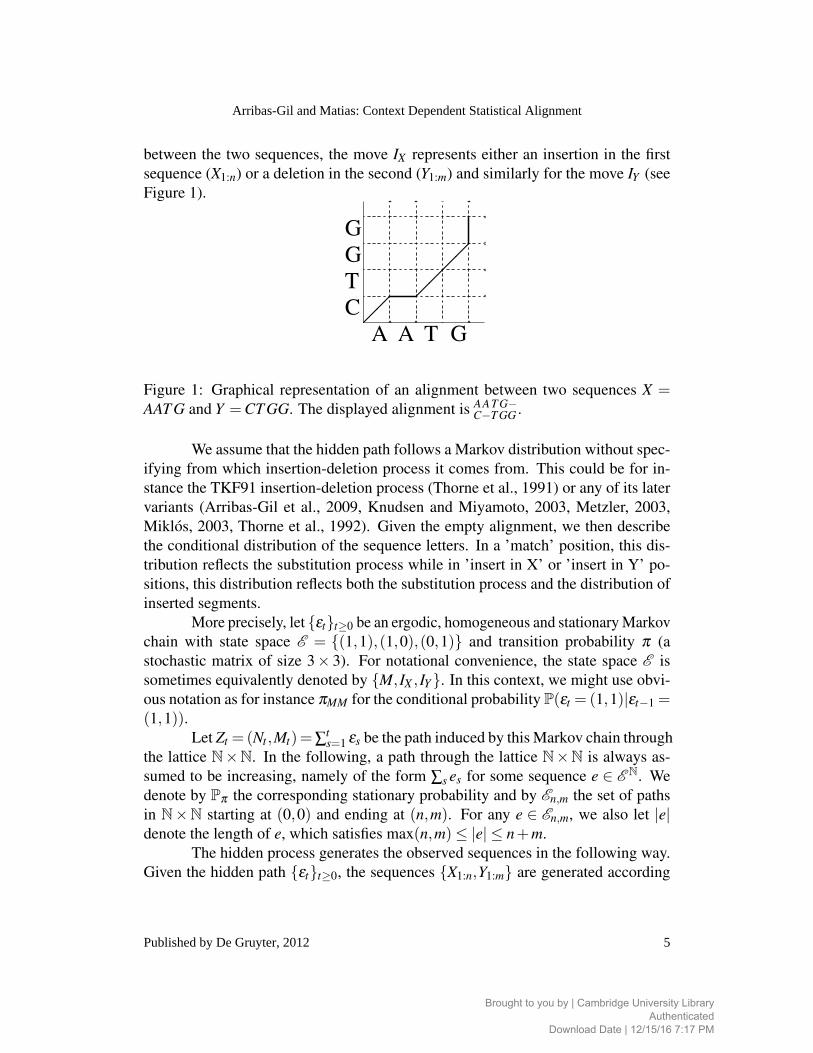
between the two sequences, the move IX represents either an insertion in the first

sequence (X1:n) or a deletion in the second (Y1:m) and similarly for the move IY (see

Figure 1).

A A T GCTGG

��

��

Figure 1: Graphical representation of an alignment between two sequences X =AAT G and Y =CT GG. The displayed alignment is AAT G−

C−T GG .

We assume that the hidden path follows a Markov distribution without spec-

ifying from which insertion-deletion process it comes from. This could be for in-

stance the TKF91 insertion-deletion process (Thorne et al., 1991) or any of its later

variants (Arribas-Gil et al., 2009, Knudsen and Miyamoto, 2003, Metzler, 2003,

Miklos, 2003, Thorne et al., 1992). Given the empty alignment, we then describe

the conditional distribution of the sequence letters. In a ’match’ position, this dis-

tribution reflects the substitution process while in ’insert in X’ or ’insert in Y’ po-

sitions, this distribution reflects both the substitution process and the distribution of

inserted segments.

More precisely, let {εt}t≥0 be an ergodic, homogeneous and stationary Markov

chain with state space E = {(1,1),(1,0),(0,1)} and transition probability π (a

stochastic matrix of size 3× 3). For notational convenience, the state space E is

sometimes equivalently denoted by {M, IX , IY}. In this context, we might use obvi-

ous notation as for instance πMM for the conditional probability P(εt = (1,1)|εt−1 =(1,1)).

Let Zt =(Nt ,Mt)=∑ts=1 εs be the path induced by this Markov chain through

the lattice N×N. In the following, a path through the lattice N×N is always as-

sumed to be increasing, namely of the form ∑s es for some sequence e ∈ E N. We

denote by Pπ the corresponding stationary probability and by En,m the set of paths

in N×N starting at (0,0) and ending at (n,m). For any e ∈ En,m, we also let |e|denote the length of e, which satisfies max(n,m)≤ |e| ≤ n+m.

The hidden process generates the observed sequences in the following way.

Given the hidden path {εt}t≥0, the sequences {X1:n,Y1:m} are generated according

5





to an order one Markov chain: for any e ∈ En,m,

P(X1:n,Y1:m|ε = e) =|e|∏s=1

P(XNs ,YMs |es,es−1,XNs−1,YMs−1

).

Note that the indexes Ns,Ms of the observations generated at time s are random.

This is in sharp contrast with the classical hidden Markov model (HMM) and is

specific to pair-HMMs (see Arribas-Gil et al., 2006, for more details).

In this work, we restrict our attention to order-one Markov conditional dis-

tributions. Note that the following developments could be generalized to higher

order Markov chains at the cost of increased computational burden.

As we want to model the dependency in the substitution process only, we

further constrain the model so that the dependency occurs only in successive ho-

mologous (match) positions. We thus use the following parametrization

P(XNs ,YMs |es,es−1,XNs−1,YMs−1

)=

⎧⎪⎪⎪⎨⎪⎪⎪⎩

h(XNs ,YMs |XNs−1,YMs−1

) if es = es−1 = (1,1),h(XNs ,YMs) if es = (1,1) �= es−1,f (XNs) if es = (1,0),g(YMs) if es = (0,1),

where f ,g are probability measures (p.m.) on A ; function h is a p.m. on A 2 and hmay be viewed as a stochastic matrix on A 2.

Obvious necessary conditions for the parameters to be identifiable in this

model are the following

⎧⎨⎩

i) ∃a,b ∈A such that h(a,b) �= f (a)g(b),ii) ∃a,b,c,d ∈A such that h(a,b|c,d) �= f (a)g(b),iii) ∃a,b,c,d ∈A such that h(a,b|c,d) �= h(a,b).

(1)

The whole parameter set is then given by

Θ = {θ = (π, f ,g,h, h);θ satisfies (1)}.

Statistical alignment of two sequences consists in maximizing with respect

to θ the following criterion wn,m(θ) (Durbin et al., 1998). This criterion plays the

role of a log-likelihood in the pair-HMM. (For a discussion on the quantities playing

the role of likelihoods in pair-HMMs, see Arribas-Gil et al., 2006). For any integers

n,m≥ 1 and any observations X1:n and Y1:m, let

wn,m(θ) := logQθ (X1:n,Y1:m) := logPθ (∃s≥ 1,Zs = (n,m);X1:n,Y1:m). (2)

6


DOI: 10.2202/1544-6115.1733



The criterion wn,m is more explicitly defined as

wn,m(θ) = log( n+m

∑s=max(n,m)

∑e∈En,m,|e|=s

Pπ(ε1:s = e1:s)

×{ s

∏k=1

f (Xnk)1{ek=(1,0)}g(Ymk)

1{ek=(0,1)}h(Xnk ,Ymk)1{ek=(1,1),ek−1 �=(1,1)}

× h(Xnk ,Ymk |Xnk−1,Ymk−1

)1{ek=ek−1=(1,1)}}),where (nk,mk) =∑k

t=1 et and 1{A} is the indicator function of set A. Now, we define

the parameter estimator as

θn,m = argmaxθ∈Θ

wn,m(θ).

In the classical pair-HMM (namely without accounting for dependencies in the sub-

stitution process), consistency results for the above estimator θn,m were obtained in

Arribas-Gil et al. (2006) and are extended here to the context dependent case in

Section 3. Then in Section 4, we develop an saem algorithm to compute θn,m and

provide an a posteriori probability distribution over the set of alignments. Indeed, a

main issue is to obtain an accurate alignment of the sequences. Score-based align-

ment methods heavily rely on the Viterbi algorithm for this purpose (see Durbin

et al., 1998), which provides the most probable a posteriori alignment. However,

optimal alignments often look different from typical ones, and providing a unique

alignment as the result of the estimation procedure may not be very informative.

For this reason, it may be more interesting to provide the probability distribution of

hidden states over each pair of nucleotides from the observed sequences (for the pa-

rameter value θn,m). This can be done under the pair-HMM framework and gives us

a reliability measure of any alignment of the two sequences (see Arribas-Gil et al.,

2009).

3 Consistency results for parameter estimationIn this part, we give generalizations of results first obtained in Arribas-Gil et al.

(2006), to the context dependent pair-HMM. As the proofs follow the same lines

as in this reference, we shall omit them. We first introduce some notation and

formulate some assumptions that will be needed. For any δ > 0, we let

Θδ = {θ ∈Θ;∀k,θk ≥ δ} and Θ0 = {θ ∈Θ;∀k,θk > 0}.The true parameter value will be denoted by θ0 and is assumed to belong to the set

Θ0. Probabilities and expectations under this parameter value are denoted by P0

7





and E0, respectively. We now introduce a notation for the marginal distributions of

h and h. For any b,c ∈A , let

hX(·) := ∑a∈A

h(·,a), hY (·) := ∑a∈A

h(a, ·),

hX(·|b,c) := ∑a∈A

h(·,a|b,c), hY (·|b,c) := ∑a∈A

h(a, ·|b,c).

We then let Θmarg be a subset of parameters in Θ0 satisfying some assumptions on

the marginals of h and h.

Θmarg ={

θ ∈Θ0;∀b,c ∈A ,hX = f ,hY = g, hX(·|b,c) = f (·), hY (·|b,c) = g(·)}.

Note that for instance, the parametrization used in Section 5 satisfies θ ∈ Θmarg.

Finally, we introduce the process wt defined in a similar way as in (2) by

wt(θ) := logQθ (X1:Nt ,Y1:Mt ).

As previously noted, the length t of an alignment of sequences with respective sizes

n and m satisfies max(n,m)≤ t ≤ n+m. Thus, asymptotic results for t →+∞ will

imply equivalent ones for n,m→+∞. In other words, consistency results obtained

when t → +∞ are valid for long enough observed sequences, even if one does not

know the length t of the true underlying alignment. We now state the main theorem.

Theorem 1. For any θ ∈Θ0, we have

i) Renormalized log-likelihood t−1wt(θ) converges P0-almost surely and in L1,as t tends to infinity, to

w(θ) = limt→∞

1

tE0 (logQθ (X1:Nt ,Y1:Mt )) = sup

t

1

tE0 (logQθ (X1:Nt ,Y1:Mt )) .

ii) Moreover, w(θ0)≥ w(θ) and strict inequality is valid as long as at least oneof the following conditions is satisfied

A. θ ∈Θ0 and ∀λ > 0,Eθ (ε1) �= λE0(ε1),B. θ0,θ ∈Θmarg and either f �= f0 or g �= g0.

iii) The family of functions {t−1wt(θ)}t≥1 is uniformly equicontinuous on the setΘδ , for any δ > 0.

The three statements in Theorem 1 are the key ingredients to establish the

consistency of θn,m, following Wald’s classical proof (Wald, 1949) of maximum

likelihood estimators consistency (see also van der Vaart, 1998, Chapter 5). The

8


DOI: 10.2202/1544-6115.1733



most subtle part is point ii), that states some sufficient conditions under which the

maximum of the limiting function w is attained only at the true parameter value θ0.

For instance, condition A means that the main directions of the paths {Zt}t≥1 gener-

ated under the two parameter values θ and θ0 are different. As a consequence, these

two parameters may be easily distinguished from each other relying on the distribu-

tions Pθ and P0. Note that these two different cases (condition A or B satisfied) are

certainly not exhaustive and we refer to Arribas-Gil et al. (2006) for simulation re-

sults indicating that point ii) might be true under other scenarios. Note in particular

that for evolutionary models assuming that insertions and deletions happen at the

same rate, Eθ (ε1) is proportional to (1,1) for any parameter value θ . In this case,

condition A) is never satisfied and we are not able to prove that h �= h0 or h �= h0

implies strict inequality w(θ0) > w(θ). This is due to the dependency structure

on the sequences, that make it difficult to link the difference w(θ0)−w(θ) with a

Kullback-Leibler divergence between densities h and h0 or between h and h0 (see

the proof of Theorem 2 in Arribas-Gil et al., 2006, for more details).

In general, one is not interested in the full (context) pair-HMM parameters

but rather in a sub-parametrization induced by the choice of a specific evolutionary

model (see for instance the sub-parametrization proposed in Section 5). Let β →θ(β ) be a continuous parametrization from some set B to Θ. For any δ > 0, let

Bδ = θ−1(Θδ ). We assume that β0 := θ−1(θ0) belongs to Bδ for some δ > 0. We

then let

βn,m := argmaxβ∈Bδ

wn,m(θ(β )).

As well as giving results on the frequentist estimator βn,m, we consider Bayesian

estimates of the parameters. Let ν be a prior probability measure on the set Bδ .

Markov chain Monte Carlo (mcmc) algorithms approximate the random distribu-

tion νn,m, interpreted as the posterior measure given observations X1:n and Y1:m and

defined by

νn,m(dβ ) =Qθ(β )(X1:n,Y1:m)ν(dβ )∫

BδQθ(β ′)(X1:n,Y1:m)ν(dβ ′)

.

With these definitions at hand, we can now state the following corollary.

Corollary 1. If the maximizer of β → w(θ(β )) over the set Bδ is reduced to thesingleton {β0}, then we have the following results

i) βn,m converges P0-almost-surely to β0,ii) If ν puts some weight on a neighborhood of β0, then the sequence of posterior

measures νn,m converges in distribution, P0-almost surely, to the Dirac massat β0.

9





4 AlgorithmsThe approach we use here to maximize criterion (2) and provide a posterior distri-

bution on the set of alignments, given two observed sequences relies on a stochas-

tic version (Celeux and Diebolt, 1985, Diebolt and Celeux, 1993) of em algorithm

(Baum, Petrie, Soules, and Weiss, 1970, Dempster et al., 1977). This approach has

already been successfully used in Arribas-Gil et al. (2009) in a classical pair-HMM

(meaning with no context dependent substitution rates) in which case it gives re-

sults very similar to Gibbs sampling. It allows one to perform maximum likelihood

estimation in a hidden variables framework where the maximization may not be ex-

plicit or where the computation of the likelihood is otherwise computationally very

expensive, or still where the use of the classical em algorithm is not feasible (see

Appendix for details).

4.1 Forward and backward equations

We describe below the forward and backward probabilities used in the later pro-

cedures. The formulas are easily obtained by generalizing those from the classical

pair-HMM (Arribas-Gil, 2007, Durbin et al., 1998).

The forward equations are obtained as follows. For any value u ∈ E , let

E un,m = {e ∈ En,m,e|e| = u} be the set of paths ending at (n,m) with last step being

u. Then the forward probabilities are defined for any i≤ n and j ≤ m, as

αu(i, j) = Pθ (∃s≥ 1,Zs = (i, j),εs = u,X1:i,Y1: j) = ∑e∈E u

n,m

Pθ (ε = e,X1:i,Y1: j).

These forward probabilities are computed recursively in the following way.

We first set the initial values

∀u ∈ E , αu(0,−1) = αu(−1,0) = 0

∀u ∈ {IX , IY}, αu(0,0) = 0 and αM(0,0) = 1.

Then for i = 0, . . . ,n and j = 0, . . . ,m except (i, j) = (0,0), we recursively compute

αM(i, j) = Pθ (∃s≥ 1,εs = (1,1),Zs = (i, j),X1:i,Y1: j)

= ∑u∈E

Pθ (∃s≥ 1,εs = (1,1),Zs = (i, j),εs−1 = u,X1:i,Y1: j)

= h(Xi,Yj|Xi−1,Yj−1)πMMαM(i−1, j−1)+h(Xi,Yj)πIX Mα IX (i−1, j−1)

+h(Xi,Yj)πIY Mα IY (i−1, j−1), (3)

10


DOI: 10.2202/1544-6115.1733



and in the same way

α IX (i, j) = f (Xi) ∑u∈E

πuIX αu(i−1, j), α IY (i, j) = g(Yj) ∑u∈E

πuIY αu(i, j−1).

Note that the log-likelihood of the observed sequences is then simply obtained from

the forward probabilities by taking

wn,m(θ) = logPθ (∃s≥ 1,Zs = (n,m),X1:n,Y1:m)

= log(α IX (n,m)+α IY (n,m)+αM(n,m)).

Note that the forward equations could thus be used to compute the log-

likelihood of two observed sequences and a numerical optimization of this quantity

could give maximum likelihood estimates. However, such a strategy falls short as

soon as the dimension of the parameter space is not small. Indeed, the computa-

tional cost of calculating the log-likelihood for a given parameter value is O(nm),and thus the computational cost of its maximization over a grid is O(pknm), where

k is the number of parameters and p the number of values considered for each pa-

rameter.

We now describe the backward probabilities and their recursive computa-

tion. For any value u ∈ E , the backward probabilities are defined as

β u(i, j) = Pθ (Xi+1:n,Yj+1:m|∃s≥ 1,Zs = (i, j),εs = u,Xi,Yj).

We initialize these values by taking, for any u ∈ E ,

β u(n,m) = 1 and β u(n,m+1) = β u(n+1,m) = 0,

and recursively compute, for i = n, . . . ,1 and j = m, . . . ,1, except (n,m), the quan-

tities

β u(i, j)= πuMβ M(i+1, j+1){h(Xi+1,Yj+1)1u∈{IX ,IY }+ h(Xi+1,Yj+1|Xi,Yj)1u=M}+πuIX β IX (i+1, j) f (Xi+1)+πuIY β IY (i, j+1)g(Yj+1). (4)

Note that contrarily to the case of HMM, the forward-backward probabil-

ities do not give rise to the classical em strategy, as we do not obtain from these

equations the conditional expectation of the complete log-likelihood, given the two

observed sequences (see Appendix for further details).

4.2 sem and saem algorithms

The forward-backward probabilities may be used to simulate the hidden path, con-

ditional on the observed sequences. Thus, em algorithm may be replaced by sem

11





(Celeux and Diebolt, 1985) or saem (Delyon et al., 1999) procedures. Indeed, let

us explain the basic idea of these stochastic versions of em algorithm. Denoting by

Lnm the random value s≥ 1 such that Zs = (n,m) (the first and only hitting time for

the point (n,m), which is not necessarily finite), the complete log-likelihood is

logPθ (X1:n,Y1:m,Lnm,ε1:Lnm)

(see Appendix for details) and for a current parameter value θ ′, its conditional ex-

pectation can be written

Qθ ′(θ) := Eθ ′(logPθ (X1:n,Y1:m,Lnm,ε1:Lnm)|X1:n,Y1:m).

Now, the idea of these stochastic approximations is to replace the computation of

Qθ ′(θ) by an approximation obtained from the simulation (under parameter value

θ ′) of a number of hidden paths {ε1:s} in En,m, with possibly different lengths.

These paths satisfy the property that for each obtained value of s, the paths with

length s have the same occurrence probability as Pθ ′(ε|X1:n,Y1:m,Lnm = s). Note

that the length of each simulated path is random. Then the maximization with re-

spect to θ of the complete log-likelihood is done on the basis of the simulated align-

ments. As a consequence, this maximization is performed via a simple counting of

specific events and does not require numerical procedures.

In particular, iteration r of sem algorithm writes

- Simulation step: generate one hidden path er of some random length s with

the same distribution as

Pθ (r−1)(ε1:s|X1:n,Y1:m,Lnm = s).

- Maximization step: θ (r) = argmaxθ∈Θ logPθ (X1:n, Y1:m, ε = er).

And iteration r of saem algorithm writes

- Simulation step: generate m(r) hidden paths er( j), j = 1, . . . ,m(r) with re-

sulting random lengths sr, j, each one having the same distribution as

Pθ (r−1)(ε1:sr, j |X1:n,Y1:m,Lnm = sr, j).

- Stochastic approximation step: update

Qr(θ) = Qr−1(θ)+ γr

( 1

m(r)

m(r)

∑j=1

logPθ (X1:n,Y1:m,ε = er( j))−Qr−1(θ)),

where {γr}r≥1 is a decreasing sequence of positive step size and Q0(θ) =∑m(0)

j=1 logPθ (X1:n,Y1:m,ε = e0( j))/m(0) .

12


DOI: 10.2202/1544-6115.1733



- Maximization step: θ (r) = argmaxθ∈Θ Qr(θ).

The simulation step is common to both algorithms and consists in drawing

paths of some unknown length s with same distribution as Pθ (r−1)(ε1:s|X1:n,Y1:m,Lnm= s). This is performed via the backwards sampling based on the forward probabil-

ities as we now explain. We may write

Pθ (r−1)(ε1:s|X1:n,Y1:m,Lnm = s)

= Pθ (r−1)(εs|X1:n,Y1:m,Lnm = s)s−1

∏k=1

Pθ (r−1)(εk|εk+1:s,X1:n,Y1:m,Lnm = s)

= Pθ (r−1)(εs|X1:n,Y1:m,Zs = (n,m))s−1

∏k=1

Pθ (r−1)(εk|εk+1,Zk+1,X1:Nk+1,Y1:Mk+1

). (5)

The last equality comes from the following: Conditional on εk+1, the random vari-

able εk does not anymore depend on the observations after time k+2. If we more-

over condition on the variables εk+1:s and Lnm = s, then we know which point (i, j)on the lattice corresponds to Zk+1 = (n,m)−∑s

t=k+2 εt = (i, j). The values of the

observed sequence after time k+2 correspond exactly to Xi+1:n,Yj+1:m. Then con-

ditional on {εk+1:s,X1:n,Y1:m,Lnm = s}, the variable εk only depends on εk+1 (ac-

cording to the Markov property) and on the values Zk+1,X1:Nk+1,Y1:Mk+1

.

So, given εk+1, the position Zk+1 = (i, j) on the lattice and the observed

values X1:i,Y1: j, we want to sample εk from Pθ (r−1)(εk|εk+1,X1:i,Y1: j,Zk+1 = (i, j)),for k = s,s− 1, . . . ,1. Up to a renormalizing constant, each step corresponds to

sampling from Pθ (r−1)(εk,εk+1|X1:i, Y1: j, Zk+1 = (i, j)) or equivalently from πεk,εk+1

αεk((i, j)−εk+1). Then the backwards sampling is based on the following equations

- ers is sampled to be v ∈ E with probability

αv(n,m)

αM(n,m)+α IX (n,m)+α IY (n,m),

- For k < s and Zk+1 = (i, j), i > 1, j > 1, if erk+1 = M, then er

k is sampled to be

M with probability

αM(i−1, j−1)πMMh(Xi,Yj|Xi−1,Yj−1)

αM(i, j),

and to be u = IX or IY with probability

αu(i−1, j−1)πuMh(Xi,Yj)

αM(i, j).

Note that these latter probabilities are correctly renormalized according to

Equation (3).

13





- For k < s and Zk+1 = (i, j), i > 1, j > 1, if erk+1 = IX then er

k is sampled to be

u ∈ E with probability

αu(i−1, j)πuIX f (Xi)

α IX (i, j), (6)

- For k < s and Zk+1 = (i, j), i > 1, j > 1, if erk+1 = IY then er

k is sampled to be

u ∈ E with probability

αu(i, j−1)πuIY g(Yj)

α IY (i, j), (7)

- For k < s and Zk+1 = (1, j), j > 1, if erk+1 = M or IX then all the values er

l ,1≤l ≤ k are fixed to IY , otherwise er

k is sampled to be u ∈ E with probability

given by (7).

- For k < s and Zk+1 = (i,1), i > 1, if erk+1 = M or IY then all the values er

l ,1≤l ≤ k are fixed to IX , otherwise er

k is sampled to be u ∈ E with probability

given by (6).

According to Equation (5), we thus have sampled paths er satisfying the following

property.

Proposition 1. The paths e ∈ En,m sampled from the above scheme with parametervalue θ occur with probability Pθ (ε = e|X1:n,Y1:m,Lnm = |e|).

We now consider the complete log-likelihood obtained from the observed

sequences and one simulated path. We have

logPθ (X1:n,Y1:m,ε = er) = ∑u∈E

1er1=u logπu +

|er|∑k=2

∑u,v∈E 2

1erk−1=u,er

k=v logπuv

+|er|∑k=1

∑a∈A

[1erk=IX ,Xnk=a log f (a)+1er

k=IY ,Ymk=a logg(a)]

+|er|∑k=1

∑a,b∈A 2

1erk=M,Xnk=a,Ymk=b logh(a,b)

+|er|∑k=2

∑a,b,c,d∈A 4

1erk=er

k−1=M,(Xnk ,Ymk ,Xnk−1,Ymk−1

)=(a,b,c,d) log h(a,b|c,d),

14


DOI: 10.2202/1544-6115.1733



where we recall that (nk,mk) = ∑ki=1 er

i (for simplicity, we omit the subscript r).

Then in the maximization step of sem, the components of θ are updated to the

values: ∀u,v ∈ E , a,b,c,d ∈A ,

π(r)u =

Ner(u)

∑v∈E

Ner(v), π(r)

u,v =Ner(u,v)

∑w∈E

Ner(u,w), f (r)(a) =

Ner(a|IX)

∑a′∈A

Ner(a′|IX ,),

g(r)(a) =Ner(a|IY )

∑a′∈A

Ner(a′|IY ,), h(r)(a,b) =

Ner(a,b|M)

∑a′,b′∈A

Ner(a′,b′|M),

h(r)(a,b|c,d) = Ner(a,b|MM;c,d)

∑a′,b′∈A

Ner(a′,b′|MM;c,d), (8)

where we use obvious notation for the counts Ne in sequence e. Namely for any

u,v∈E , and any a,b,c,d ∈A , we let Ne(u)=∑k 1{ek = u}, Ne(u,v)=∑k 1{ek−1 =u,ek = v}, Ne(a|IX) =∑k 1{ek = IX ,XNk = a} and similarly for Ne(a|IY ), Ne(a,b|M)and also

Ne(a,b|MM;c,d) = ∑k

1{ek = ek−1 = M,(XNk ,YMk ,XNk−1,YMk−1

) = (a,b,c,d)}.

In the maximization step of saem we have to take into account the m(r)hidden paths and the stochastic approximation of Qr(θ). Then the values of θ are

updated as in (8) by replacing the counts Ner(·) by their counterparts Nr(·), where

Nr = Nr−1 + γr

(∑m(r)

j=1 Ner( j)− Nr−1

)/m(r).

From a theoretical point of view, the convergence properties of the two al-

gorithms are different. In saem, the sequence {θ r}r≥1 converges, under general

conditions, to a local maximum of the log-likelihood. It is important to note that

the stochastic perturbation introduced with respect to the original em algorithm al-

lows avoiding saddle points, which are possible attractive stationary points of the

sequence generated by em (Delyon et al., 1999). In sem, the sequence {θ r}r≥1 does

not converge pointwise, but it is an homogeneous Markov chain which is ergodic

under appropriate conditions, see for instance Diebolt and Ip (1996).

In this context, maximum likelihood estimators are sensitive to overfitting

if there is insufficient data. Indeed, if an event has never been observed in the se-

quences, the corresponding estimator is not well defined, as both the numerator and

denominator in (8) are zero. Pseudo-counts (Durbin et al., 1998, Chapter 3) or other

smoothing techniques such as the one proposed in Kneser and Ney (1995) may be

used to solve this problem. However, when using saem algorithm to perform maxi-

mum likelihood estimation, this problem is minimized and no smoothing strategies

15





are required. Indeed, since at iteration r we generate m(r) hidden paths, the counts

Nr (computed as an average over those alignments) are rarely equal to 0, even during

the first iterations when γr is typically set to 1. However, if we want to completely

avoid this possibility, we may replace event counts by pseudo-counts in the case

of unobserved events, during these first iterations. Note also that in practice we do

not generate whole alignments at each iteration step, but only sub-alignments of a

certain given length within the current alignment. This strategy combines an mcmc

procedure within saem and is known to preserve convergence properties of saem al-

gorithm (see Arribas-Gil et al., 2009, for further details). In terms of event counts,

this strategy implies that a current low estimate of an event occurrence probability

will have some impact on next iteration estimate. Nonetheless, at the last iterations

of the algorithm, when typically γr < 1, current counts are averaged with counts

from previous iterations, which provides a smoothing procedure by itself.

Note that very efficient HMM tools such as the compiler described in Lunter

(2007) could be used to implement our model and the algorithms described above.

The code we used to produce the results of the next sections was written in FORTRAN

95 and may be obtained from the first author upon request.

5 SimulationsFor these simulations, we consider nucleotide sequences with alphabet A = {A,C,G,T} and a constrained parameter set, motivated by the choice of an underlying

evolutionary model on these sequences. As for the generation of the hidden Markov

chain, we consider the TKF91 indel model with equal value for insertion and dele-

tion rate λ (see Arribas-Gil, 2007, for more details). The transition matrix of the

hidden path is thus given by

π =1

1+λ

⎛⎜⎜⎜⎝

e−λ 1− e−λ λλe−λ

1− e−λ λ 1+λ − λ1− e−λ

e−λ 1− e−λ λ

⎞⎟⎟⎟⎠ ,

where the order of the states in the matrix is M, IX and IY . Then, we describe the

conditional distribution of the sequences. For any x ∈A , we set f (x) = g(x) = μx,

where μ is going to be the stationary distribution of the substitution process, ac-

cording to the parametrization of h and h considered below. We set the distribution

h according to a simple substitution process with equal substitution rate γ and dif-

ferent nucleotides frequencies (modified Jukes Cantor). Let

h(x,y) ={

μx(1− e−γ)μy if x �= yμx[μx(1− e−γ)+ e−γ ] if x = y.

16


DOI: 10.2202/1544-6115.1733



Table 1: Parameter values in the two data sets.Data set 1 α = 0.4 β = 0.2 γ = 0.06 λ = 0.04

Data set 2 α = 0.5 β = 0.15 γ = 0.05 λ = 0.02

The parameter h accounting for the context in the substitution process differs from

h only in a CC match context. In this way, we want to take into account a possibly

higher substitution rate from the pair CpG to CpA. More precisely, we let

P(XNs = x,YMs = y|es = es−1 = M,XNs−1= x′,YMs−1

= y′)

=

{hC(x,y) if x′ = y′ =C,h(x,y) otherwise.

In a CC match context, we use a model initially introduced in two slightly differ-

ent forms by Felsenstein (1984) and Hasegawa, Kishino, and Yano (1985). This

model considers different substitution rates for transitions (i.e. substitutions within

the chemical class of purines R = {A,G} or pyrimidines Y = {C,T}) and for

transversions (substitutions modifying the chemical class) as well as different nu-

cleotide frequencies μ . Denoting by x the other nucleotide in the same chemical

class as x (namely x �= x and either {x, x} ∈R or {x, x} ∈ Y ), we get

hC(x,y) =

⎧⎪⎨⎪⎩

μxe−(α+β ) +μxe−β (1− e−α) μxμx+μx

+μx(1− e−β )μx if y = x,μxe−β (1− e−α) μx

μx+μx+μx(1− e−β )μx if y = x,

μx(1− e−β )μy otherwise.

We refer to Felsenstein (2003) for more details on substitution processes.

According to this parametrization we have simulated two sets of data with

an alignment length of 2000 base pairs (bp) and parameter values described in Ta-

ble 1. In these data sets, the substitution rate γ is larger than the indel rate λ as

expected in biological sequences, and the transition and transversion substitution

rates in a CC match context (α and β ) are larger than the regular substitution rate γ .

In both sets of data we have set the stationary distribution of the substitution process

to

μA = 0.225 μC = 0.275 μG = 0.275 μT = 0.225,

in order to obtain a GC content (proportion of Gs or Cs) larger than 50%.

For each one of the data sets we have conducted two estimation procedures.

On the one hand, we have estimated the whole parameter (π, f ,g,h, h) via the saem

algorithm as explained in Section 4.2. On the other hand, we have combined the

17





saem algorithm with numerical optimization to estimate only the evolutionary pa-

rameters λ , γ , α and β . The first procedure has the advantages of being robust

against misspecification of the underlying evolutionary model and relying on a

explicit maximization step based on the counts of events. The second procedure

is computationally more expensive, however, it is more parsimonious and it pro-

vides a straightforward evolutionary interpretation of the parameter values. In both

cases we have performed 150 iterations of the saem algorithm with the parameter

γr of the stochastic approximation set to 1 for r = 1, . . . ,100 and to 1/(r−100) for

r = 101, . . . ,150. The number of simulated hidden paths is m(r) = 5, r = 1, . . . ,20

and m(r) = 10, r = 21, . . . ,150. We used the same initial values of the parameters

for every simulation run over the two simulated data sets. Note that we first tried

different sets of initial values and these had almost no impact on the convergence of

the algorithms. These initial values, estimates and standard deviations are given in

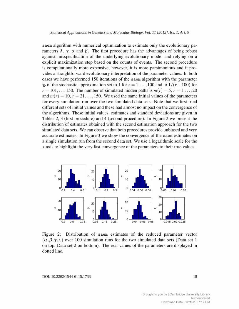
Tables 2, 3 (first procedure) and 4 (second procedure). In Figure 2 we present the

distribution of estimates obtained with the second estimation approach for the two

simulated data sets. We can observe that both procedures provide unbiased and very

accurate estimates. In Figure 3 we show the convergence of the saem estimates on

a single simulation run from the second data set. We use a logarithmic scale for the

x-axis to highlight the very fast convergence of the parameters to their true values.

0.2 0.4 0.60

10

20

α

0.1 0.2 0.30

10

20

β

0.04 0.06 0.080

10

20

γ

0.03 0.04 0.050

10

20

λ

0.3 0.5 0.750

10

20

α

0.05 0.15 0.250

10

20

β

0.04 0.06 0.080

10

20

γ

0.015 0.02 0.0250

10

20

30

λ

Figure 2: Distribution of saem estimates of the reduced parameter vector

(α,β ,γ,λ ) over 100 simulation runs for the two simulated data sets (Data set 1

on top, Data set 2 on bottom). The real values of the parameters are displayed in

dotted line.

18


DOI: 10.2202/1544-6115.1733



Table 2: Mean values and standard deviations of estimates over 100 simulation runs

for Data Set 1. The estimation has been performed without taking into account the

specific parametrization used to generate the data.Initial value True value Estimate (sd)

πMM 0.85 0.9238 0.9184 (0.0101)

πMIX 0.075 0.0377 0.0407 (0.0074)

πMIY 0.075 0.0385 0.0410 (0.0077)

πIX M 0.85 0.9424 0.8807 (0.0998)

πIX IX 0.075 0.0385 0.0387 (0.0308)

πIX IY 0.075 0.0191 0.0805 (0.1034)

πIY M 0.85 0.9238 0.8788 (0.0982)

πIY IX 0.075 0.0377 0.0821 (0.0987)

πIY IY 0.075 0.0385 0.0391 (0.0305)

h(A,A) 0.0625 0.2148 0.2155 (0.0109)

h(A,C) 0.0625 0.0036 0.0031 (0.0019)

h(A,G) 0.0625 0.0036 0.0032 (0.0019)

h(A,T ) 0.0625 0.0029 0.0027 (0.0018)

h(C,A) 0.0625 0.0036 0.0034 (0.0021)

h(C,C) 0.0625 0.2634 0.2628 (0.0130)

h(C,G) 0.0625 0.0044 0.0044 (0.0024)

h(C,T ) 0.0625 0.0036 0.0034 (0.0021)

h(G,A) 0.0625 0.0036 0.0030 (0.0017)

h(G,C) 0.0625 0.0044 0.0041 (0.0023)

h(G,G) 0.0625 0.2634 0.2653 (0.0120)

h(G,T ) 0.0625 0.0036 0.0032 (0.0018)

h(T,A) 0.0625 0.0029 0.0026 (0.0016)

h(T,C) 0.0625 0.0036 0.0031 (0.0017)

h(T,G) 0.0625 0.0036 0.0035 (0.0021)

h(T,T ) 0.0625 0.2148 0.2166 (0.0113)

hC(A,A) 0.0625 0.1600 0.1626 (0.0169)

hC(A,C) 0.0625 0.0112 0.0108 (0.0053)

hC(A,G) 0.0625 0.0446 0.0454 (0.0111)

hC(A,T ) 0.0625 0.0092 0.0091 (0.0051)

hC(C,A) 0.0625 0.0112 0.0102 (0.0056)

hC(C,C) 0.0625 0.2055 0.2072 (0.0193)

hC(C,G) 0.0625 0.0137 0.0126 (0.0056)

hC(C,T ) 0.0625 0.0446 0.0429 (0.0108)

hC(G,A) 0.0625 0.0446 0.0440 (0.0098)

hC(G,C) 0.0625 0.0137 0.0140 (0.0061)

hC(G,G) 0.0625 0.2055 0.2050 (0.0174)

hC(G,T ) 0.0625 0.0112 0.0110 (0.0053)

hC(T,A) 0.0625 0.0092 0.0086 (0.0047)

hC(T,C) 0.0625 0.0446 0.0456 (0.0106)

hC(T,G) 0.0625 0.0112 0.0111 (0.0062)

hC(T,T ) 0.0625 0.1600 0.1598 (0.0197)

19






for Data set 2. The estimation has been performed without taking into account the

specific parametrization used to generate the data.Initial value True value Estimate (sd)

πMM 0.85 0.9610 0.9559 (0.0071)

πMIX 0.075 0.0194 0.0221 (0.0051)

πMIY 0.075 0.0196 0.0219 (0.0055)

πIX M 0.85 0.9706 0.8477 (0.1262)

πIX IX 0.075 0.0196 0.0199 (0.0221)

πIX IY 0.075 0.0098 0.1323 (0.1289)

πIY M 0.85 0.9610 0.8407 (0.1321)

πIY IX 0.075 0.0194 0.1367 (0.1379)

πIY IY 0.075 0.0196 0.0226 (0.0252)

h(A,A) 0.0625 0.2165 0.2168 (0.0114)

h(A,C) 0.0625 0.0030 0.0027 (0.0015)

h(A,G) 0.0625 0.0030 0.0027 (0.0014)

h(A,T ) 0.0625 0.0025 0.0024 (0.0015)

h(C,A) 0.0625 0.0030 0.0026 (0.0017)

h(C,C) 0.0625 0.2653 0.2673 (0.0122)

h(C,G) 0.0625 0.0037 0.0033 (0.0020)

h(C,T ) 0.0625 0.0030 0.0027 (0.0016)

h(G,A) 0.0625 0.0030 0.0023 (0.0015)

h(G,C) 0.0625 0.0037 0.0033 (0.0020)

h(G,G) 0.0625 0.2653 0.2643 (0.0096)

h(G,T ) 0.0625 0.0030 0.0023 (0.0013)

h(T,A) 0.0625 0.0025 0.0024 (0.0015)

h(T,C) 0.0625 0.0030 0.0025 (0.0016)

h(T,G) 0.0625 0.0030 0.0027 (0.0015)

h(T,T ) 0.0625 0.2165 0.2196 (0.0102)

hC(A,A) 0.0625 0.1588 0.1595 (0.0159)

hC(A,C) 0.0625 0.0086 0.0069 (0.0038)

hC(A,G) 0.0625 0.0505 0.0504 (0.0096)

hC(A,T ) 0.0625 0.0071 0.0067 (0.0042)

hC(C,A) 0.0625 0.0086 0.0087 (0.0045)

hC(C,C) 0.0625 0.2053 0.2053 (0.0199)

hC(C,G) 0.0625 0.0105 0.0103 (0.0046)

hC(C,T ) 0.0625 0.0505 0.0504 (0.0101)

hC(G,A) 0.0625 0.0505 0.0515 (0.0102)

hC(G,C) 0.0625 0.0105 0.0097 (0.0052)

hC(G,G) 0.0625 0.2053 0.2036 (0.0191)

hC(G,T ) 0.0625 0.0086 0.0078 (0.0043)

hC(T,A) 0.0625 0.0071 0.0078 (0.0041)

hC(T,C) 0.0625 0.0505 0.0515 (0.0098)

hC(T,G) 0.0625 0.0086 0.0084 (0.0040)

hC(T,T ) 0.0625 0.1588 0.1613 (0.0166)

20


DOI: 10.2202/1544-6115.1733




for the two data sets. The estimation has been performed by numerical optimization

on the reduced parameter vector (α,β ,γ,λ ).Data set 1

Initial value True value Estimate (sd)

α 0.8 0.4 0.400 (0.0750)

β 0.25 0.2 0.1985 (0.0372)

γ 0.1 0.06 0.0602 (0.0087)

λ 0.08 0.04 0.0402 (0.0040)

Data set 2

Initial value True value Estimate (sd)

α 0.8 0.5 0.5091 (0.0772)

β 0.25 0.15 0.1493 (0.0296)

γ 0.1 0.05 0.0499 (0.0079)

λ 0.08 0.02 0.0196 (0.0024)

100 101 1020.4

0.5

0.6

0.7

0.8

0.9

1

α

100 101 102

0.15

0.2

0.25

β

100 101 1020

0.1

0.2

0.3

0.4

γ

100 101 1020

0.02

0.04

0.06

0.08

λ

Figure 3: saem estimates of the reduced parameter vector (α,β ,γ,λ ) over iterations

in a single simulation run from the second data set. A logarithmic scale is used for

the x-axis. The true parameter values are displayed in dotted line.

6 Application to real dataIn this section we illustrate our method through an alignment of the human alpha-

globin pseudogene (HBPA1) with its functional counterpart, the human alpha-globin

gene (HBA1). This example is inspired by the work of Bulmer (1986), who studied

the neighbouring base effects on substitution rates in a series of vertebrate pseudo-

genes, including the human alpha-globin, concluding that there is an increase in the

frequency of substitutions from the dinucleotide CpG.

21





We have extracted the sequences of the gene and the pseudogene, that are

located in the human alpha-globin gene cluster on chromosome 16, from the UCSC

Genome Browser database (Fujita, Rhead, and Zweig, 2010). We have considered

the whole sequences (coding and non-coding sequence in the case of the functional

gene) for the alignment, obtaining sequences lengths of 842 bp for HBA1 and 812

bp for HBPA1. Because of the presence of introns and exons in the HBA1 sequence,

it is natural to consider a model allowing for two different substitution behaviors

along the sequence. That is why we have used a model for which the state space

of the hidden Markov chain is {M1,M2, IX , IY}, where Mi, i = 1,2, stand for two

different match states, with different associated substitution processes hi, hi, i= 1,2.

This kind of model may also handle fragments insertion and deletion in contrast to

single nucleotide indels (see Arribas-Gil et al., 2009, for more details). As in the

simulation studies of the previous section, h is the substitution matrix in a CC match

context, and h is the substitution matrix in any other case. In this way, we want to

take into account a possibly higher transition rate from nucleotide G occurring in the

dinucleotide CpG. In order to avoid any possible misspecification of the underlying

indel and substitution processes, we have decided not to parametrize any of those,

conducting an estimation approach equivalent to the first procedure described in

the previous section. The only difference here lies in the dimension of the model

parameter, since this parameter is now (π, f ,g,h1,h2, h1, h2), where π is a 4× 4

transition probability matrix, and hi, hi, i = 1,2 are four different 4× 4 stochastic

vectors, yielding a total number of 12+3+3+4×15 = 78 free parameters.

We have run saem algorithm on the sequences, performing 500 iterations

with γr set to 1 for r = 1, . . . ,400 and to 1/(r− 400) for r = 401, . . . ,500. The

number of simulated hidden paths is m(r) = 5, r = 1, . . . ,20 and m(r) = 10, r =21, . . . ,500. In Table 5, we present the estimated substitution probabilities from

nucleotide G. As expected, we found an increase in the substitution occurrence for

G in a CC match context. We present in Figure 4 the posterior probability distribution

over the set of possible alignment columns, match, insertion and deletion (the two

match states have been merged) for every pair of aligned positions in a consensus

alignment obtained at the convergence stage (last iterations) of saem algorithm.

In order to compare our method to a traditional pair-HMM alignment, we

have also run saem algorithm, with the same settings as before, on a simpler model

without substitution context-dependence. In this model we consider again two dif-

ferent substitution regimes, so the parameter vector is now (π, f ,g,h1,h2), yielding

a total number of 12+3+3+2×15 = 48 free parameters. We present in Figure 5

the posterior probability distribution over the set of possible alignment columns,

match, insertion or deletion (the two match states have been merged) for every pair

of aligned positions in a consensus alignment obtained at the convergence stage

(last iterations) of saem algorithm. This posterior probability is quite similar to the

22


DOI: 10.2202/1544-6115.1733



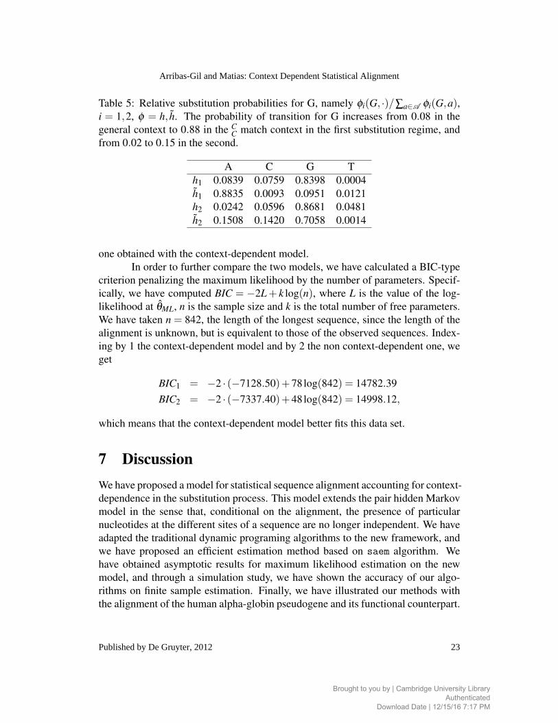
Table 5: Relative substitution probabilities for G, namely φi(G, ·)/∑a∈A φi(G,a),i = 1,2, φ = h, h. The probability of transition for G increases from 0.08 in the

general context to 0.88 in the CC match context in the first substitution regime, and

from 0.02 to 0.15 in the second.

A C G T

h1 0.0839 0.0759 0.8398 0.0004

h1 0.8835 0.0093 0.0951 0.0121

h2 0.0242 0.0596 0.8681 0.0481

h2 0.1508 0.1420 0.7058 0.0014

one obtained with the context-dependent model.

In order to further compare the two models, we have calculated a BIC-type

criterion penalizing the maximum likelihood by the number of parameters. Specif-

ically, we have computed BIC = −2L+ k log(n), where L is the value of the log-

likelihood at θML, n is the sample size and k is the total number of free parameters.

We have taken n = 842, the length of the longest sequence, since the length of the

alignment is unknown, but is equivalent to those of the observed sequences. Index-

ing by 1 the context-dependent model and by 2 the non context-dependent one, we

get

BIC1 = −2 · (−7128.50)+78log(842) = 14782.39

BIC2 = −2 · (−7337.40)+48log(842) = 14998.12,

which means that the context-dependent model better fits this data set.

7 DiscussionWe have proposed a model for statistical sequence alignment accounting for context-

dependence in the substitution process. This model extends the pair hidden Markov

model in the sense that, conditional on the alignment, the presence of particular

nucleotides at the different sites of a sequence are no longer independent. We have

adapted the traditional dynamic programing algorithms to the new framework, and

we have proposed an efficient estimation method based on saem algorithm. We

have obtained asymptotic results for maximum likelihood estimation on the new

model, and through a simulation study, we have shown the accuracy of our algo-

rithms on finite sample estimation. Finally, we have illustrated our methods with

the alignment of the human alpha-globin pseudogene and its functional counterpart.

23





100 200 300 400 500 600 700 8000

0.5

1

M

100 200 300 400 500 600 700 8000

0.5

1

IX

100 200 300 400 500 600 700 8000

0.5

1

IY

Figure 4: Posterior probability distribution of the alignment states at the maximum

likelihood parameter estimate with the substitution context-dependent model.

We have compared the new model with a classical pair-HMM through a model se-

lection criterion, concluding that taking into account the context-dependence on the

substitution process may improve the fitting of the data. However, this might of

course not be the case with all data sets and regarding to the increase in the model

complexity, we recommend to use context dependent alignment only when there is

biological evidence of a role of dependent substitutions. It should be noted that or-

der one dependency in the substitution process might be insufficient to capture many

biological phenomena. While this work could be generalized to handle higher order

Markov conditional distributions, this would have a non negligible computational

cost. Among possible extensions of this work, a very promising one lies in combin-

ing our approach with the pair-TAG proposal of Hickey and Blanchette (2011a,b) to

handle dependency in the substitution process as well as in the indel one. We stress

that both approaches (pair-HMMs and pair-TAGs) are restricted to the alignment of

two homologous sequences, and that it would be interesting to include these context

dependencies in multiple statistical alignment procedures.

Appendix: The need for a stochastic approximationLet us explain why em algorithm may not be applied in pair-HMM. Denoting by

Lnm the random value s≥ 1 such that Zs = (n,m) (the first and only hitting time for

24


DOI: 10.2202/1544-6115.1733



100 200 300 400 500 600 700 8000

0.5

1

M

100 200 300 400 500 600 700 8000

0.5

1

IX

100 200 300 400 500 600 700 8000

0.5

1

IY

Figure 5: Posterior probability distribution of the alignment states at the maxi-

mum likelihood parameter estimate without taking into account possible substitu-

tion context-dependence.

the point (n,m), which is not necessarily finite), the complete log-likelihood writes

logPθ (X1:n,Y1:m,Lnm,ε1:Lnm) =n+m

∑s=max(n,m)

1Lnm=s

{∑

u∈E

1ε1=u logπu

+s

∑k=2

∑u,v∈E 2

1εk−1=u,εk=v logπuv

+s

∑k=1

∑a∈A

[1εk=IX ,XNk=a log f (a)+1εk=IY ,YMk=a logg(a)]

+s

∑k=1

∑a,b∈A 2

1εk=M,εk−1 �=M,XNk=a,YMk=b logh(a,b)

+s

∑k=2

∑a,b,c,d∈A 4

1εk=εk−1=M,(XNk ,YMk ,XNk−1,YMk−1

)=(a,b,c,d) log h(a,b|c,d)}.

To simplify notation, we let X := X1:n,Y :=Y1:m,L := Lnm and Fs = {X,Y,L = s}.Moreover, we let (ε,X ,Y )k :=(εk,XNk ,YMk). Taking the expectation of the complete

log-likelihood, conditional on the observed sequences, under a current parameter

25





value θ ′, leads to

Eθ ′(logPθ (X,Y,L,ε1:L)|X,Y)

=n+m

∑s=max(n,m)

Pθ ′(L = s|X,Y){

∑u∈E

Pθ ′(ε1 = u|Fs) logπu

+s

∑k=2

∑u,v∈E 2

Pθ ′((εk−1,εk) = (u,v)|Fs) logπuv

+s

∑k=1

∑a∈A

[Pθ ′((ε,X)k = (IX ,a)|Fs) log f (a)+Pθ ′((ε,Y )k = (IY ,a)|Fs) logg(a)

]

+s

∑k=1

∑a,b

Pθ ′(εk−1 �= M,(ε,X ,Y )k = (M,a,b)|Fs) logh(a,b)

+s

∑k=2

∑a,b,c,d

Pθ ′((εk,εk−1,(X ,Y )k,(X ,Y )k−1) = (M,M,a,b,c,d)|Fs)

× log h(a,b|c,d)}.

There are two main issues at stake here. First, the quantity Pθ ′(Lnm|X1:n,Y1:m) is not

given by the forward-backward equations. Second, computing this conditional ex-

pectation would also require the knowledge of Pθ ′(εk−1,εk|X,Y,L = s). However,

the forward backward equations rather give access to quantities as for instance

α IX (i−1, j−1)πIX Mh(Xi,Yj)β M(i, j) = Pθ (εk−1 = IX ,εk = M|X,Y,Zk = (i, j)).

In other words, the conditional distribution of (εk−1,εk) is known only conditional

on the extra knowledge of the position Zk of the path in the lattice at time k. In con-

clusion, in pair-HMM, the forward-backward equations are not sufficient to com-

pute the expectation of the complete log-likelihood, conditional on the observed

sequences.

ReferencesArribas-Gil, A. (2007): Estimation dans des modeles a variables cachees : aligne-

ment de sequences biologiques et modeles d’evolution, Ph.D. thesis, Universite

Paris-Sud, France, http://halweb.uc3m.es/esp/Personal/personas/aarribas/esp/

docs/these_arribas_gil.pdf.

Arribas-Gil, A., E. Gassiat, and C. Matias (2006): “Parameter estimation in pair-

hidden Markov models,” Scand J Stat, 33, 651–671.

26


DOI: 10.2202/1544-6115.1733



Arribas-Gil, A., D. Metzler, and J.-L. Plouhinec (2009): “Statistical alignment with

a sequence evolution model allowing rate heterogeneity along the sequence,”

IEEE/ACM Transactions on Computational Biology and Bioinformatics, 6, 281–

295.

Baum, L., T. Petrie, G. Soules, and N. Weiss (1970): “A maximization technique

occurring in the statistical analysis of probabilistic functions of Markov chains.”

Ann Math Stat, 41, 164–171.

Bulmer, M. (1986): “Neighboring base effects on substitution rates in pseudo-

genes,” Mol Biol Evol, 3, 322–329.

Celeux, G. and J. Diebolt (1985): “The SEM algorithm: a probabilistic teacher al-

gorithm derived from the EM algorithm for the mixture problem,” ComputationalStatistics Quaterly, 2, 73–82.

Delyon, B., M. Lavielle, and E. Moulines (1999): “Convergence of a stochastic

approximation version of the EM algorithm,” Ann Stat, 27, 94–128.

Dempster, A., N. Laird, and D. Rubin (1977): “Maximum likelihood from incom-

plete data via the EM algorithm.” J Roy Stat Soc B, 39, 1–38.

Dewey, C. N., P. M. Huggins, K. Woods, B. Sturmfels, and L. Pachter (2006):

“Parametric alignment of Drosophila genomes,” PLoS Comput Biol, 2, e73.

Diebolt, J. and G. Celeux (1993): “Asymptotic properties of a stochastic EM al-

gorithm for estimating mixing proportions,” Comm Statist. Stochastic Models, 9,

599–613.

Diebolt, J. and E. H. S. Ip (1996): “Stochastic EM: method and application,” in

Markov chain Monte Carlo in practice, Interdiscip. Statist., London: Chapman

& Hall, 259–273.

Durbin, R., S. Eddy, A. Krogh, and G. Mitchison (1998): Biological sequenceanalysis: probabilistic models of proteins and nucleic acids, Cambridge, UK:

Cambridge University Press.

Felsenstein, J. (1984): “Distance methods for inferring phylogenies: A justifica-

tion,” Evolution, 38, pp. 16–24.

Felsenstein, J. (2003): Inferring phylogenies, Sinauer Associates.

Fujita, P. A., B. Rhead, and A. A. et al.. Zweig (2010): “The UCSC Genome

Browser database: update 2011,” Nucleic Acids Res.Gambin, A., J. Tiuryn, and J. Tyszkiewicz (2006): “Alignment with context depen-

dent scoring function,” J Comput Biol, 13, 81–101.

Gambin, A. and P. Wojtalewicz (2007): “CTX-BLAST: context sensitive version of

protein BLAST,” Bioinformatics, 23, 1686–1688.

Hasegawa, M., H. Kishino, and T.-A. Yano (1985): “Dating of the human-ape split-

ting by a molecular clock of mitochondrial DNA,” J Mol Evol, 22, 160–174.

27





¨

´

in Computational Molecular Biology, Lecture Notes in Computer Science, vol-

ume 6577, Springer Berlin / Heidelberg, 85–103.

Hickey, G. and M. Blanchette (2011b): “A probabilistic model for sequence align-

ment with context-sensitive indels,” J Comput Biol., 18, 1449–1464.

Hobolth, A. (2008): “A Markov chain Monte Carlo Expectation Maximization

algorithm for statistical analysis of DNA sequence evolution with neighbor-

dependent substitution rates.” Journal of Computational and Graphical Statis-tics, 17, 138–162.

Holmes, I. (2005): “Using evolutionary Expectation Maximization to estimate indel

rates.” Bioinformatics, 21, 2294–2300.

Holmes, I. and W. Bruno (2001): “Evolutionary HMMs: A Bayesian approach to

multiple alignment,” Bioinformatics, 17, 803–820.

Holmes, I. and R. Durbin (1998): “Dynamic programming alignment accuracy,” JComput Biol., 5, 493–504.

Huang, X. (1994): “A context dependent method for comparing sequences,” in

Combinatorial pattern matching (Asilomar, CA, 1994), Lecture Notes in Comput.Sci., volume 807, Berlin: Springer, 54–63.

Jukes, T. H. and C. R. Cantor (1969): “Evolution of protein molecules,” in

H. Munro, ed., Mammalian Protein Metabolism III, Academic Press, New York.,

21–132.

Kneser, R. and H. Ney (1995): “Improved backing-off for m-gram language model-

ing,” in Proceedings of the IEEE International Conference on Acoustics, Speech,and Signal Processing, volume 1, volume 1, 181–184.

Knudsen, B. and M. Miyamoto (2003): “Sequence alignments and pair hidden

Markov models using evolutionary history.” J Mol Biol, 333, 453–460.

Loytynoja, A. and N. Goldman (2008): “A model of evolution and structure for

multiple sequence alignment,” Philosophical Transactions of the Royal SocietyB: Biological Sciences, 363, 3913–3919.

Lunter, G. (2007): “HMMoC - a compiler for hidden Markov models,” Bioinfor-matics, 23, 2485–2487.

Lunter, G., A. J. Drummond, I. Miklos, and J. Hein (2005): “Statistical alignment:

Recent progress, new applications, and challenges,” in R. Nielsen, ed., StatisticalMethods in Molecular Evolution, Statistics for Biology and Health, Springer New

York, 375–405.

Lunter, G., A. Rocco, N. Mimouni, A. Heger, A. Caldeira, and J. Hein (2007): “Un-

certainty in homology inferences: Assessing and improving genomic sequence

alignment,” Genome Res, 18, 000.

Hickey, G. and M. Blanchette (2011a): “A probabilistic model for sequence align-

ment with context-sensitive indels,” in V. Bafna and S. Sahinalp, eds., Research

28


DOI: 10.2202/1544-6115.1733



from a poisson sequence length distribution,” Discrete Appl Math, 127, 79 – 84,

computational Molecular Biology Series - Issue IV.

Miklos, I., G. Lunter, and I. Holmes (2004): “A ’Long Indel’ model for evolutionary

sequence alignment,” Mol Biol Evol, 21, 529–540.

Miklos, I. and Z. Toroczkai (2001): “An improved model for statistical alignment,”

in O. Gascuel and B. Moret, eds., Algorithms in Bioinformatics, Lecture Notes inComputer Science, volume 2149, Springer Berlin / Heidelberg, 1–10.

Siepel, A. and D. Haussler (2004): “Computational identification of evolutionarily

conserved exons,” in Proceedings of the eighth annual international conferenceon Research in computational molecular biology, RECOMB ’04, New York, NY,

USA: ACM, 177–186.

Thorne, J., H. Kishino, and J. Felsenstein (1991): “An evolutionary model for max-

imum likelihood alignment of DNA sequences.” J Mol Evol, 33, 114–124.

Thorne, J., H. Kishino, and J. Felsenstein (1992): “Inching toward reality: an im-

proved likelihood model of sequence evolution.” J Mol Evol, 34, 3–16.

van der Vaart, A. W. (1998): Asymptotic statistics, Cambridge Series in Statisticaland Probabilistic Mathematics, volume 3, Cambridge: Cambridge University

Press.

Varela, M. and W. Amos (2009): “Evidence for nonindependent evolution of adja-

cent microsatellites in the human genome,” J Mol Evol, 68, 160–170.

Wald, A. (1949): “Note on the consistency of the maximum likelihood estimate,”

Ann. Math. Statistics, 20, 595–601.

Waterman, M. S. and M. Eggert (1987): “A new algorithm for best subsequence

alignments with application to tRNA-rRNA comparisons,” J Mol Biol, 197, 723

– 728.

Wong, K. M., M. A. Suchard, and J. P. Huelsenbeck (2008): “Alignment uncertainty

and genomic analysis,” Science, 319, 473–476.

Metzler, D. (2003): “Statistical alignment based on fragment insertion and deletion

models.” Bioinformatics, 19, 490–499.

Miklos, I. (2003): “Algorithm for statistical alignment of two sequences derived

29





Documents

Statistical Applications in Genetics and Molecular Biologycmatias.perso.math.cnrs.fr/Docs/SAGMB_Arribas_Matias.pdf · Volume 11, Issue 1 2012 Article 5 Statistical Applications in